Seigniorage and distortionary taxation in a model

with heterogeneous agents and idiosyncratic

uncertainty∗

Sofia Bauducco†

JOB MARKET PAPER

November 2008

Abstract

In this paper we study the optimal monetary and fiscal policy mix in a model in which

agents are subject to idiosyncratic uninsurable shocks to their labor productivity. We identify

two main effects of anticipated inflation absent in representative agent frameworks. First,

inflation stimulates savings for precautionary reasons. Hence, a higher level of anticipated

inflation implies a higher capital stock in steady state, which translates into higher wages and

lower taxes on labor income. This benefits poor, less productive agents. Second, inflation

acts as a regressive consumption tax, which favors rich and productive agents. We calibrate

our model economy to the U.S. economy and compute the optimal policy mix. We find

that, for a utilitarian government, the Friedman rule is optimal even when we allow for the

presence of heterogeneity and uninsurable idiosyncratic risk. Although the aggregate welfare

costs of inflation are small, individual costs and benefits are large. Net winners from inflation

are poor, less productive agents, while middle-class and rich households are always net losers.

JEL Classification: E52, E63, E21, D31.

Keywords: Seigniorage, Friedman rule, Heterogeneous Agents, Optimal Monetary and

Fiscal Policy

∗I would like to thank Albert Marcet and Josep Pijoan-Mas for fruitful discussions and solid guidance. I

also want to thank Klaus Adam, Anton Braun, Andrea Caggese, Francesco Caprioli, Juan Carlos Conesa, Jose

Dorich, Andres Erosa, Jordi Gali, Antonio Mele, Michael Reiter, Thijs Van Rens and seminar participants at

the UPF Macro Break and CEMFI Lunchtime Seminar for useful comments and suggestions. All errors are my

responsibility.†Email: sofia.bauducco@upf.edu

1

1 Introduction

The seminal papers by Friedman (1969) and Phelps (1973) opened a wide debate in the last

decades over the issue of the optimal monetary and fiscal policy combination in representative

agent frameworks. Friedman argued that optimality required setting the nominal interest rate

to zero, so that the return on money holdings was equated to the return on any other interest-

bearing nominal asset. This is known in the literature as the Friedman rule. Phelps, on the other

hand, indicated that in economies in which lump-sum taxes are not available, the policy maker

should tax all goods, including money. Moreover, since the money demand function is typically

more inelastic than the demand for consumption goods, Phelps concluded that money should be

taxed heavily. This apparent contradiction in the optimal policy prescription motivated some

classical papers such as Chari et al. (1996) and Correia and Teles (1996) among many others.

With some exceptions, the general consensus appears to be that Central Banks should follow

the Friedman rule.

However, by construction all these early contributions overlook issues of heterogeneity and

redistribution. By working with the representative agent assumption their analysis of optimal

policy focuses only on efficiency in distorting relative prices. Therefore, a crucial aspect of

inflation is neglected, which is the fact that it does not affect all individuals in the same way.

In this paper we tackle this issue by building a heterogeneous agent model with uninsurable

idiosyncratic shocks to labor productivity. We consider the problem of a benevolent government

that has to finance an exogenous and constant stream of public expenditure. The available

instruments are the inflation tax and a tax on labor income and, given that labor supply is

endogenous, both instruments are distortionary. We look for the determination of the optimal

monetary and fiscal policy mix in such an environment, assuming the government assigns equal

weight to all agents in the economy1.

Since we are interested in identifying and studying the effects of inflation over individuals

with different income and wealth profiles, we need a model in which agents differ in these two

dimensions. In order to assess the effect exerted by inflation on the incentives of households

to consume, work and save, and consequently on aggregate long-run capital and output, we

depart from the complete-markets assumption by assuming that agents cannot insure against

their idiosyncratic shocks and are subject to a borrowing constraint. Finally, previous literature

has pointed to the fact that inflation can be regarded as a regressive tax on consumption2. We

1Examples of other papers that use the same social welfare function are Domeij and Heathcote (n.d.), Floden

(2001), Floden and Linde (2001) and Heathcote et al. (2008a).2See Erosa and Ventura (2002).

2

introduce this in the analysis by means of a transaction technology alternative to money in which

richer, more productive agents have comparative advantages relative to poorer, less productive

ones. In addition, we exacerbate these advantages by assuming easier access to the transaction

technology for more productive agents.

In the setup we propose there are two effects from inflation that are not present in representative-

agent frameworks. On the one hand, more productive agents, by having easier access to alterna-

tive transaction technologies, can shelter better from inflation. This shifts the burden of taxation

from richer, more productive agents to poorer households, thus benefiting the former group. If

the planner cares sufficiently for poor agents, this effect goes in favor of the Friedman rule.

On the other hand, in economies in which households cannot insure against their idiosyncratic

shocks, inflation amplifies the motive for precautionary savings. When the bad shock hits and

the individual is very poor (i.e., is close to hitting the borrowing constraint) the inflation tax re-

duces consumption and leisure and, consequently, utility, thus creating an incentive to save. The

higher savings level translates into higher capital in steady state, higher wages and lower labor

tax rates. By this means, a higher level of inflation increases welfare of poor, low productivity

households that rely almost entirely on labor income. When the government cares about poor

households, this effect goes against the Friedman rule. Considering these two effects jointly, we

see that they operate in opposite directions. Deviating from the Friedman rule assures poor

agents a higher labor income, while middle-class and rich agents have to endure lower levels of

capital income. Nevertheless, they are benefited by a reduction in their tax burden associated

to the increase in the inflation tax which, as explained before, is a regressive tax.

There is a distortion associated to inflation that is already present in environments with a

representative agent, which is related to the uniform taxation argument from the public finance

literature. When consumption goods can be bought either with cash or with an alternative

transaction technology, deviating from the Friedman rule implies taxing the goods bought with

cash more than the rest of the goods. If all goods enter in the utility function of the household

in identical manner, this is not efficient3.

From the previous discussion it can be concluded that, in economies with uninsurable id-

iosyncratic uncertainty and heterogeneous agents, the determination of the optimal monetary

and fiscal policy mix remains a quantitative question. In order to provide a suitable answer,

we calibrate the model economy to match some selected statistics of the U.S. economy. Some

key targets are the correlation between money and asset holdings, the fraction of consump-

3To be more precise, for this argument to hold the utility function has to be separable in consumption and

leisure and the subutility over consumption goods has to be homothetic.

3

tion expenditures made with cash and the Gini coefficient of the asset distribution. We define

the benchmark economy to be one that displays an annual rate of inflation of 2%, which is a

reasonable annual inflation target for the Fed.

Given our parameterization we find that for a utilitarian planner4 the Friedman rule is

optimal despite the introduction of heterogeneity and uninsurable idiosyncratic risk. The afore-

mentioned beneficial effects of inflation on welfare are not sufficiently large, from a quantitative

point of view, to offset its detrimental effects. Thus the Friedman rule is optimal. Next, we per-

form a welfare analysis comparing the benchmark economy to an economy in which the Friedman

rule is implemented. we find that the aggregate welfare gains of switching from the benchmark

policy regime to the optimal one are rather small. The percent of life-time consumption that

agents in the benchmark economy are prepared to give up to get the policy change is 0.51%.

Following Floden (2001) we decompose these welfare gains into gains from increased levels of

consumption, reduced uncertainty and reduced inequality. We find that most of the gains are

due to increased levels of consumption and, to a lesser extent, to reduced uncertainty.

Despite these seemingly small aggregate welfare gains, the individual welfare gains and loses

can be very large. A surprising finding is that poor, less productive agents are net losers from

the policy change5. When inflation decreases, so does aggregate capital and, with it, wages.

This effect can be very harmful for these agents: we find that, for the poorest individual,

consumption should decrease permanently by about 4% in the benchmark economy for him

to be indifferent between living in any of the two worlds proposed. On the contrary, middle-

class and rich individuals are net winners from the change in regime. Rich, low- productivity

households should obtain a permanent increase in consumption of around 4% to be indifferent

between the two regimes. These large individual effects cancel out almost completely in the

aggregate, thus yielding the small overall effects described before.

Although this paper is not the first one to look at inflation in heterogeneous-agent envi-

ronments, it is, to our knowledge, the first one that identifies in a unified framework different

effects of inflation that had been described separately and derives the optimal policy within such

framework.

The contributions of Erosa and Ventura (2002) and Algan and Ragot (2006) study the

redistributive aspects of inflation. Both papers point out to different mechanisms through which

inflation affects the welfare of agents depending on their level of wealth and labor productivity,

namely, that inflation acts as a regressive tax on consumption and that it stimulates savings.

4A utilitarian planner is one that assigns equal weights to all households in the computation of the social

welfare function.5See Algan and Ragot (2006) for a similar result.

4

They reach contradictory conclusions: while the former states that inflation is relatively more

harmful to poorer households, the latter claims that the higher level of capital in steady state

translates into higher wages and higher welfare for poor, labor-income dependent individuals.

Neither of these papers addresses the issue of inflation from a normative point of view.

There are a number of papers that deal with the determination of the optimal inflation rate

when taking into account issues of heterogeneity. Akyol (2004) studies an endowment economy

in which only high productivity households hold money in equilibrium. Seigniorage revenues can

be used to finance redistributive (anonymous) transfers and interest payments on government

debt. Therefore, the main role of inflation is to redistribute resources from agents with high

endowment shocks to those holding bonds, which improves risk-sharing. The author finds that

the optimal inflation rate is of about 10%. Although in this paper not all high-productivity

agents are also rich, the correlation between wealth and productivity is very high. Then, the

idea that richer agents are the ones holding money en equilibrium is at odds with some stylized

facts on transactions and cash holdings reported in Erosa and Ventura (2002), which indicate

the opposite. In this paper, we construct the model such that its predictions in terms of cash

holdings and proportion of purchases made with cash are in line with what the data suggests.

Albanesi (2005) and Bhattacharya et al. (2007) propose frameworks in which agents are

ex-ante heterogeneous and there is no idiosyncratic uncertainty. In particular, they assume

there are two types of households in the economy. Albanesi (2005) finds that it may be optimal

to depart from Friedman rule, depending on the weight that the government assigns to each

type of agent. On the other hand, Bhattacharya et al. (2007) conclude that, because inflation

redistributes resources from one type of agent to the other, both types may benefit if the central

bank deviates from the Friedman rule. Both papers abstract from capital, but given the lack

of idiosyncratic uninsurable risk, monetary policy would not affect the long-run capital stock.

This is a crucial aspect of inflation that we include in our analysis.

Some papers in the search literature study the implications of anticipated inflation, as for

example Lagos and Rocheteau (2005) and Bhattacharya et al. (2005). These studies view mone-

tary policy as a mechanism to induce agents to exert the correct amount of search effort. Search

effort is related to the quantity of output produced and, consequently, welfare. The scope of

this literature is substantially different from ours. Although I do regard money as a means of

payment, my interest in inflation is related to the fact that it distorts the consumption, leisure

and savings decisions. Thus, we do not address in detail how money facilitates transactions and

to what extent monetary policy can enhance this role but, rather, focus on the effects of money

growth on allocations.

5

Finally, da Costa and Werning (2008) propose a framework in which agents have private

information on their labor productivity. The analysis abstracts from idiosyncratic risk by as-

suming that differences in productivity are permanent. Moreover, agents do not hold capital.

The authors assume that money and work effort are complements, so that the demand for money,

conditional on the expenditure of goods, weakly increases with the amount of work effort. They

find that the Friedman rule is optimal if labor income is positively taxed. The reason for this re-

sult is that deviating from the Friedman rule does not aid the planner in designing a mechanism

to ensure that individuals do not underreport their productivity, i.e., it does not help relaxing

the incentive-compatibility constraints in the planner’s problem. Although this study and ours

reach similar conclusions in terms of policy prescription, the reasons behind this result are very

different in the two setups. We assume the government cannot observe an agent’s productivity

by restricting the set of fiscal instruments to an anonymous tax on labor, so in our framework

agents do not have incentives to underreport by construction. Instead, we focus on the effects

of inflation on households that differ in wealth as well as labor productivity.

The remainder of the paper is organized as follows. Section 2 describes the model. In section

3 we discuss the calibration strategy. Section 4 contains a description of the different effects

operating in the model and shows the results in terms of optimal policy. In section 5 we perform

the welfare analysis. Finally, section 6 concludes and discusses lines for future research.

2 The model

The model is close to Erosa and Ventura (2002) but with two important differences. First, in

our model the labor supply is endogenous. Second, we introduce the idea that more productive

agents have easier access to transaction technologies alternative to the use of cash, with respect

to less productive agents. These two modifications to the basic setup alter completely the

analysis of the effects of inflation over different population sectors. We defer the discussion of

these effects until the next section.

There is no aggregate uncertainty. Households face idiosyncratic labor productivity shocks,

that we denote by εt. Consequently, the economy is at its steady state and all aggregate variables

remain constant. For simplicity, we will omit the time subscript from aggregate real variables.

2.1 Households

The economy is populated by a continuum of mass 1 of ex-ante identical and infinitely lived

households. Households are endowed with one unit of time each period and derive utility from

6

consumption of final goods and leisure.

Markets are incomplete, in the sense that it is not possible to trade bonds which payoffs

are contingent on the realization of the idiosyncratic shock. Moreover, we assume that agents

cannot borrow. Consequently, agents can only save by holding one-period riskless assets and

money. We denote by Wt the total nominal wealth an individual has in period t, where Wt is

the sum of total money holdings Mt and assets At.

Agents consume a continuum of final goods indexed by j ∈ [0, 1]. We assume that the

consumption aggregator, denoted by c, takes the form c = infj{c(j)}6. The choice of the

aggregator implies that agents consume an equal amount of each good j, therefore

c = c(j) = c(m) ∀j,m ∈ [0, 1]

Agents choose optimally whether to buy final goods with cash or with a costly transaction

technology, which we will call credit. In order to buy an amount c of good j with credit, the

consumer must purchase γ(j) units of financial services.

Following Lucas and Stokey (1983), we assume that the financial market closes first and the

goods market follows. More specifically, at the beginning of period t, after observing the current

shock εt, agents adjust their portfolio compositions by trading money and assets in a centralized

securities market and pay the credit obligations that they contracted in the previous period. In

this sense, the transaction technology we consider does not allow households to transfer liabilities

from one period to the other. Instead, it represents a way in which consumers can transform

their interest-bearing assets into a means of payment that is not subject to the inflation tax.

The gross nominal return of a one-period bond At is the nominal interest rate R. Notice

that the gross nominal return of money is 1, so money is (weakly) dominated in rate of return

by assets. Nevertheless, households value money because it provides liquidity services to buy

consumption goods.

After trade in the securities market has taken place, the goods market opens. At this stage,

households buy consumption goods with money or credit, decide how much to work and save

a fraction of their total income in the form of nominal wealth Wt+1 that they will carry to the

next period to transform it into assets and money in the securities market. Household i’s budget

constraint at the time the goods market opens is

ptcit + qt

∫ zit

0

γi(j)dj +W it+1 = RAi

t +M it + (1 − τ l)ωpt(1 − lit)ε

it (1)

6We choose this aggregator for simplicity reasons only. Working with a more general aggregator such as a

Dixit-Stigliz aggregator does not alter our results qualitatively.

7

where pt is the unitary price of the final good, qt is the price of a unit of financial services,∫ zi

t

0γi(j)dj is the total amount of credit bought, ω is the real wage for one efficiency unit of

labor, lit is time devoted to leisure and τ l is an anonymous linear tax on labor income.

As mentioned before, households need either cash or credit in order to buy consumption

goods. Agents choose which goods they will buy with credit and which with cash, and zit ∈ [0, 1]

stands for the fraction of goods bought with credit by household i7. Since all goods that are not

bought with credit need to be paid with money, household i faces the following cash-in-advance

constraint in the goods market:

ptcit(1 − zi

t) ≤M it (2)

Notice that, if R > 1, money is strictly dominated in rate of return by assets and, conse-

quently, constraint (2) will always be binding because agents can adjust their money holdings

after the idiosyncratic shock is observed.

The problem that household i solves can be stated as

max E0

∞∑

t=0

βtu(cit, lit)

subject to

ptcit + qt

∫ zit

0

γi(j)dj +W it+1 = RAi

t +M it + (1 − τ l)ωpt(1 − lit)ε

it

ptcit(1 − zi

t) ≤M it

Ait ≥ 0

In the appendix we show the optimality conditions associated to this problem.

2.2 Firms

There are two types of competitive firms in this economy: firms that produce consumption goods

and financial firms that produce transaction services. We assume that all markets are perfectly

competitive and, in consequence, firms make zero profits in equilibrium.

7To be more precise, agents will buy goods indexed from 0 to zit with credit and the rest of the goods (from

zit to index 1) with cash.

8

2.2.1 Consumption goods sector

Let K denote the aggregate capital stock and Lg aggregate labor in efficiency units employed

in the goods sector. Then the production technology in the consumption goods sector can be

written as

yt = F (K,Lg)

where F (·) is a neoclassical production function8. Optimality conditions of the firm are

r = FK − δ (3)

ω = F gL (4)

where r is the before-tax real return on capital and δ is the depreciation rate.

2.2.2 Financial services sector

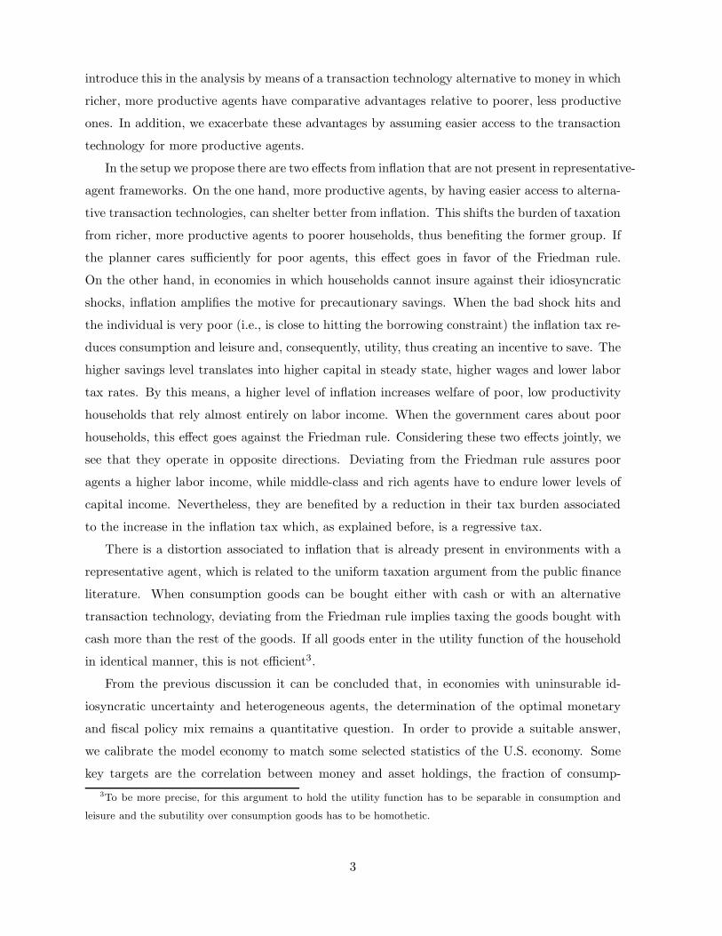
We assume that a household with labor productivity εit can acquire a fraction of goods zit with

credit at zero marginal cost, and that zit depends on the potential labor income of an agent.

More specifically, zit = f(εit) with

∂zit

εit

> 0. In words, this assumption means that the fraction of

goods that can be purchased with credit at zero marginal cost increases with the productivity

of an agent. Then, more productive agents have an advantage in the use of credit with respect

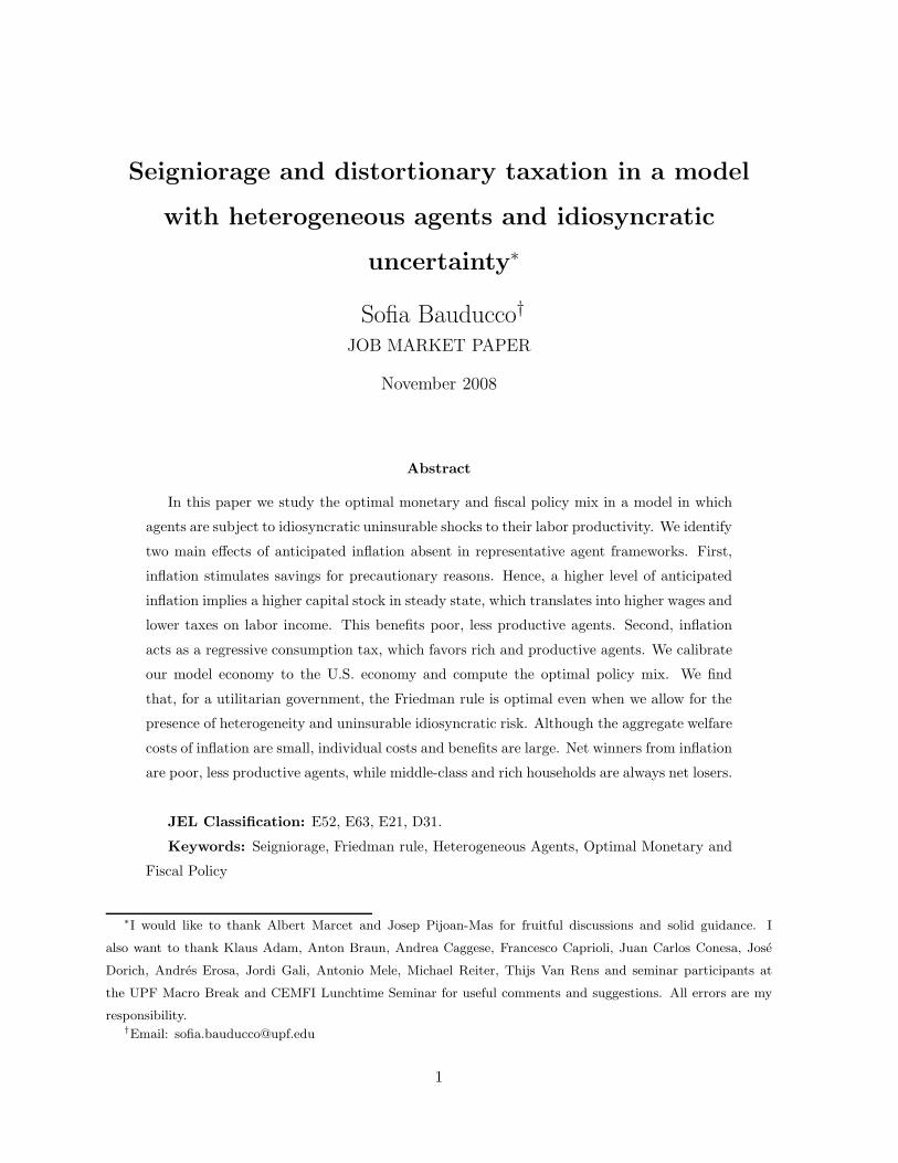
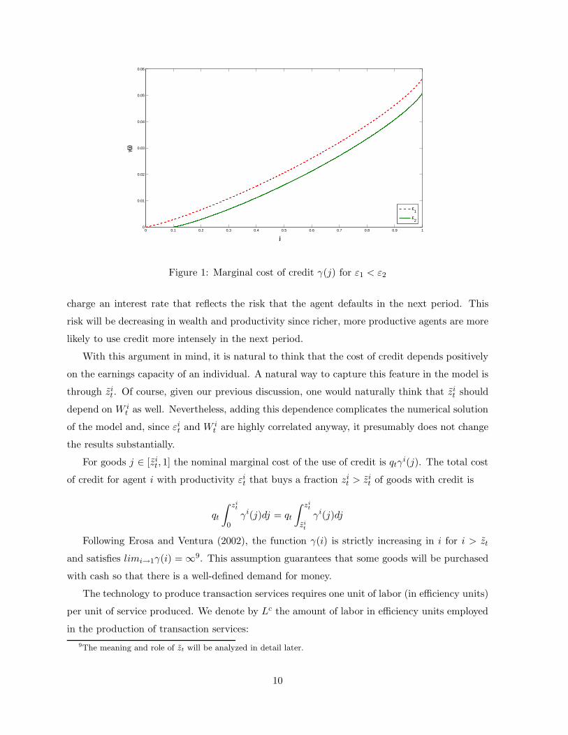
to less productive ones. Figure 1 shows the marginal cost of credit for goods i ∈ [0, 1] for agents

n and m with εnt > εmt .

The assumption that zit depends positively on the labor productivity of agent i is a shortcut

to reflect the better access to commercial credit markets that high-income, rich households enjoy

when compared to poor, low-income ones. Think of a similar scenario to the one proposed here,

but now at the beginning of each period, after observing her individual shock, household i

decides whether to repay her credit obligations contracted in the last period. If the household

chooses not to repay she is excluded from the credit market for the next period, otherwise it can

apply for a new credit line. The household will decide to pay the credit obligations contracted in

period t− 1 only if the value of the credit in t is higher or equal than what she owes from t− 1.

Obviously, the amount of credit in t is determined by the wealth and the labor productivity

of the agent in t. In t − 1, when the agent applies for the loan, the financial services firm will

8We assume that the production function is identical for any type of consumption good i ∈ [0, 1] so the relative

price of any two types of goods i and j is 1 ∀i, j.

9

0 0.1 0.2 0.3 0.4 0.5 0.6 0.7 0.8 0.9 10

0.01

0.02

0.03

0.04

0.05

0.06

j

γ(j)

ε1

ε2

Figure 1: Marginal cost of credit γ(j) for ε1 < ε2

charge an interest rate that reflects the risk that the agent defaults in the next period. This

risk will be decreasing in wealth and productivity since richer, more productive agents are more

likely to use credit more intensely in the next period.

With this argument in mind, it is natural to think that the cost of credit depends positively

on the earnings capacity of an individual. A natural way to capture this feature in the model is

through zit. Of course, given our previous discussion, one would naturally think that zi

t should

depend on W it as well. Nevertheless, adding this dependence complicates the numerical solution

of the model and, since εit and W it are highly correlated anyway, it presumably does not change

the results substantially.

For goods j ∈ [zit, 1] the nominal marginal cost of the use of credit is qtγ

i(j). The total cost

of credit for agent i with productivity εit that buys a fraction zit > zi

t of goods with credit is

qt

∫ zit

0

γi(j)dj = qt

∫ zit

zit

γi(j)dj

Following Erosa and Ventura (2002), the function γ(i) is strictly increasing in i for i > zt

and satisfies limi→1γ(i) = ∞9. This assumption guarantees that some goods will be purchased

with cash so that there is a well-defined demand for money.

The technology to produce transaction services requires one unit of labor (in efficiency units)

per unit of service produced. We denote by Lc the amount of labor in efficiency units employed

in the production of transaction services:

9The meaning and role of zt will be analyzed in detail later.

10

∫ ∫ zit

zit

γi(j)djdλ = Lc

where λ is the distribution of agents in the economy. Firms in the sector charge the price

qt per unit of credit sold. Competition ensures that firms make zero profits and set their prices

such that ωpt = qt10.

2.3 Government

There is a benevolent government that has to finance an exogenous stream of public spending

through distortionary taxes on aggregate labor income and asset returns and through seigniorage

revenues. The nominal budget constraint of the government is

ptg +Mt = τ lωptL+ τkrptK +Mt+1 (5)

where L is total aggregate labor in efficiency units L = Lg + Lc and τk is the tax rate on

asset returns.

2.4 Equilibrium

In our economy, each agent is characterized by the pair (wt, εt) where wt is wealth in real

terms. Let W ≡ [0, w] be the compact set of all possible wealth holdings where w is an upper

bound on wealth and the lower bound is determined by the no borrowing condition11. Let

E ≡ {ε1, ε2, ..., εn} be the set of all possible realizations of the labor productivity shock εt. The

shock follows a Markov process with transition probabilities π(ε′, ε) = Pr(εt+1 = ε′|εt = ε).

Define the state space S as the cartesian product S = W ×E with Borel σ-algebra B and typical

subset S = (W × E). The space (S,B) is a measurable space, and for any set S ∈ B λ(S) is

the measure of agents in the set S. Denote Λ as the set of all probability measures over (S,B).

Then,

10The zero profit condition can be written as

qt

Z Z zi

t

0

γ(j)djdλ = ptωLc

11Notice that the no borrowing condition means that

at ≥ 0 (6)

Nevertheless, since wt = at + mt and at and mt are decision variables of the agent, only by imposing wt ≥ 0

we make sure that condition (6) is satisfied always.

11

λt+1(W × E) =

∫

S

Q((w, ε),W × E)dλt(w, ε)

where Q((w, ε),W × E) is the probability that an individual with current state (w, ε) is in

the set W × E next period:

Q((w, ε),W × E) =∑

ε′∈E

I{w′(w, ε) ∈ W}π(ε′, ε)

Here I(·) is the indicator function and w′(w, ε) is the optimal savings policy of an individual

in state (w, ε).

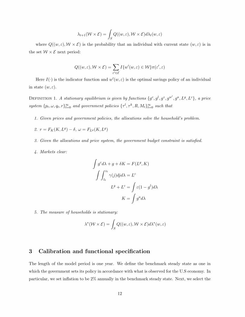
Definition 1. A stationary equilibrium is given by functions {gc, gl, gz, gw′, ga, Lg, Lc}, a price

system {pt, ω, qt, r}∞t=0 and government policies {τ l, τk, R,Mt}

∞t=0 such that

1. Given prices and government policies, the allocations solve the household’s problem.

2. r = FK(K,Lg) − δ, ω = FLg (K,Lg)

3. Given the allocations and price system, the government budget constraint is satisfied.

4. Markets clear:

∫

gcdλ+ g + δK = F (Lg,K)

∫ ∫ zt

zt

γ(j)djdλ = Lc

Lg + Lc =

∫

ε(1 − gl)dλ

K =

∫

gadλ

5. The measure of households is stationary:

λ∗(W × E) =

∫

S

Q((w, ε),W × E)dλ∗(w, ε)

3 Calibration and functional specification

The length of the model period is one year. We define the benchmark steady state as one in

which the government sets its policy in accordance with what is observed for the U.S economy. In

particular, we set inflation to be 2% annually in the benchmark steady state. Next, we select the

12

model parameters so that in the benchmark steady state equilibrium the model economy matches

some selected features of the U.S data. While some of the parameters can be set externally,

others are estimated within the model and require solving for equilibrium allocations12. We

summarize the values of externally set and internally calibrated parameters in Tables 3.1.2 and

3.2.1, as well as the targets they are related to and the values for the targets obtained from the

model. Notice that, in the case of internally determined parameters, all parameters affect all

calibration targets. Nevertheless, since usually each parameter affects more directly only one

target, we report in the table the target that it is more related to13.

3.1 Parameters set exogenously

3.1.1 Preferences

Following Domeij and Floden (2006), the utility function we use is

u(ct, ll) =c1−σt − 1

1 − σ− θ0

(1 − lt)1+

1

θ1

1 + 1

θ1

(7)

This specification is convenient because the Frisch elasticity of labor supply is equal to θ1.

We set θ1 = 0.59, which is in line with Domeij and Floden (2006) estimates14. It is common to

find in the literature that σ ∈ [1, 2], so we set σ = 1.515.

3.1.2 Technology

Consumption goods sector: The technology for the production of consumption goods is a

standard Cobb-Douglas function

y = KαLg1−α

α is set such that the labor income share of GDP, wL/Y = 1 − α = 0.64.

12The distinction between externally set and internally calibrated parameters corresponds to Heathcote et al.

(2008b).13As Pijoan-Mas (2006) explains, this calibration strategy can be seen as an exactly identified simulated method

of moments estimation.14These authors claim that previous estimates of the labor-supply elasticity are inconsistent with incomplete

market models because borrowing constraints are not considered in the analysis, in particular, they are downward-

biased.15Examples of papers that use these values are Erosa and Ventura (2002), Campanale (2007), Castaneda et al.

(2003) and Domeij and Heathcote (n.d.), among many others.

13

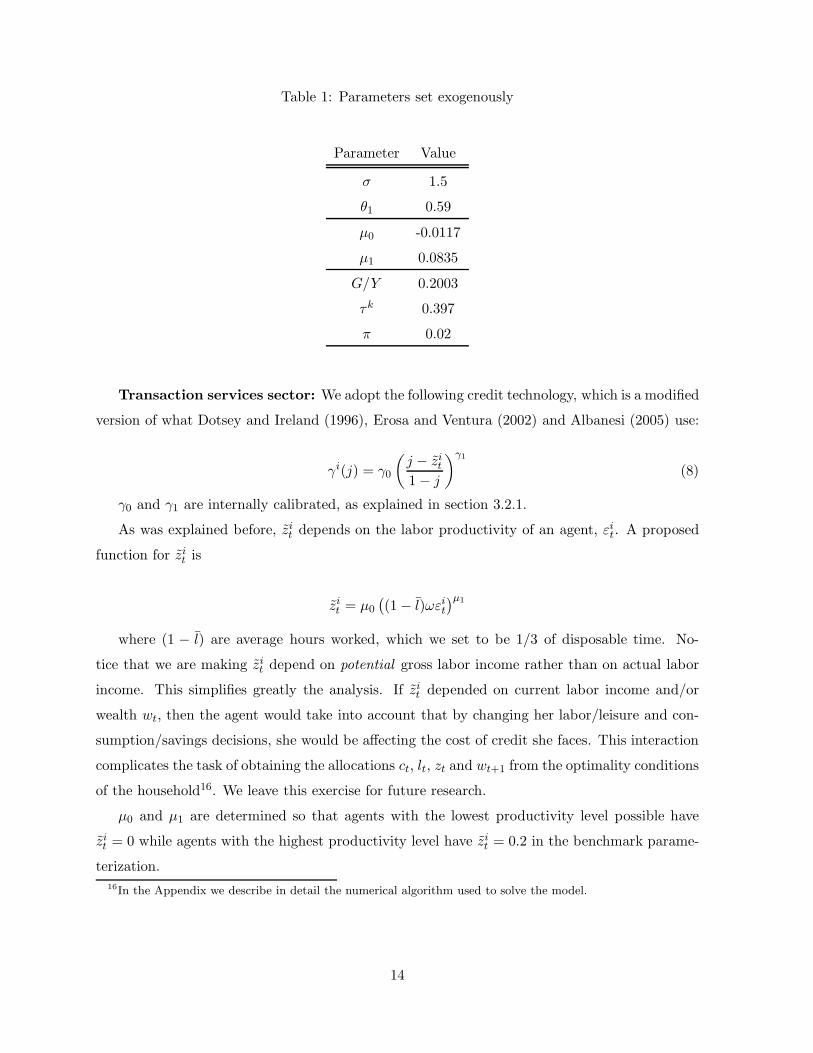
Table 1: Parameters set exogenously

Parameter Value

σ 1.5

θ1 0.59

µ0 -0.0117

µ1 0.0835

G/Y 0.2003

τk 0.397

π 0.02

Transaction services sector: We adopt the following credit technology, which is a modified

version of what Dotsey and Ireland (1996), Erosa and Ventura (2002) and Albanesi (2005) use:

γi(j) = γ0

(

j − zit

1 − j

)γ1

(8)

γ0 and γ1 are internally calibrated, as explained in section 3.2.1.

As was explained before, zit depends on the labor productivity of an agent, εit. A proposed

function for zit is

zit = µ0

(

(1 − l)ωεit)µ1

where (1 − l) are average hours worked, which we set to be 1/3 of disposable time. No-

tice that we are making zit depend on potential gross labor income rather than on actual labor

income. This simplifies greatly the analysis. If zit depended on current labor income and/or

wealth wt, then the agent would take into account that by changing her labor/leisure and con-

sumption/savings decisions, she would be affecting the cost of credit she faces. This interaction

complicates the task of obtaining the allocations ct, lt, zt and wt+1 from the optimality conditions

of the household16. We leave this exercise for future research.

µ0 and µ1 are determined so that agents with the lowest productivity level possible have

zit = 0 while agents with the highest productivity level have zi

t = 0.2 in the benchmark parame-

terization.

16In the Appendix we describe in detail the numerical algorithm used to solve the model.

14

3.1.3 Government

We adopt a very standard parameterization for fiscal variables. Usually it is accepted that the

ratio of government expenditure over GDP lies in the interval [0.19, 0.22]17 . We set G/Y =

0.2. To make our study comparable to other papers in the optimal fiscal policy literature, we

introduce a tax on asset returns τk. Nevertheless, we assume it is fixed at a value of 0.397,

which is in line with Domeij and Heathcote (n.d.) and Floden and Linde (2001). The reason to

introduce this tax is that, otherwise, almost all public revenues would have to come from labor

income taxation, causing the distortion on the labor/leisure decision to be very large. Finally,

we set inflation to be 0.02 in the benchmark parameterization.

3.2 Internally calibrated parameters

3.2.1 Preferences and technology

We need to pin down θ0 from the utility function (7), the discount factor β, the depreciation

rate δ and the two parameters γ0 and γ1 from the credit technology (8). The targets we choose

are the following: the average fraction of disposable time devoted to work should be 1/318,

the capital to output ratio should be K/Y = 319, the investment to output ratio should be

I/Y = 0.25, the correlation between money and asset holdings should be corr(m,a) = 0.1620

and the fraction of consumption expenditures made with cash should be∫

(1 − zit)c

itdλ = 0.821.

3.2.2 Labor productivity process

Our main aim is to define what the optimal mix of fiscal and monetary policy should be in the

presence of idiosyncratic uninsurable risk. As we will see in the following sections, individuals

with different levels of wealth and labor income are affected differently by different policies.

Moreover, the optimal policy prescription depends crucially on the presence and the extent in

17Some studies that use values in this range are Erosa and Ventura (2002), Campanale (2007) and Floden and

Linde (2001).18See Pijoan-Mas (2006) and Castaneda et al. (2003) for a similar choice.19Pijoan-Mas (2006), Campanale (2007), Conesa and Krueger (1999) and Castaneda et al. (2003)among others.20The correlation between money and asset holdings is computed using the 2004 Survey of Consumer Finances.

Since cash holdings are not reported in the survey, we use the amount of money held in checking accounts as a

proxy for money holdings. All the remaining sources of net worth are considered to be assets at.21Erosa and Ventura (2002) report that 80% of transactions are made with cash (M1). Since we do not have

a measure of the number of transactions in our model, we use as a proxy the value of transactions. Similarly,

Algan and Ragot (2006) report that M1/C ≃ 0.78 for the 1960-2000 period. We use a value of 0.8 which is in

the middle of these two.

15

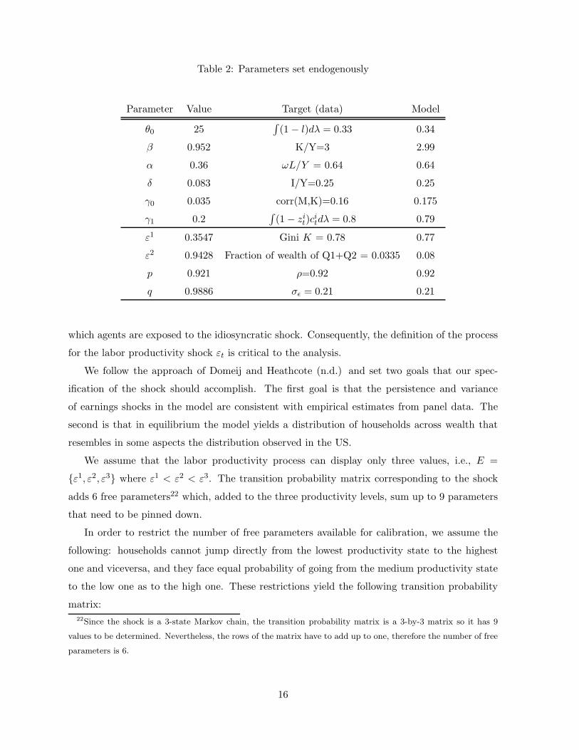
Table 2: Parameters set endogenously

Parameter Value Target (data) Model

θ0 25∫

(1 − l)dλ = 0.33 0.34

β 0.952 K/Y=3 2.99

α 0.36 ωL/Y = 0.64 0.64

δ 0.083 I/Y=0.25 0.25

γ0 0.035 corr(M,K)=0.16 0.175

γ1 0.2∫

(1 − zit)c

itdλ = 0.8 0.79

ε1 0.3547 Gini K = 0.78 0.77

ε2 0.9428 Fraction of wealth of Q1+Q2 = 0.0335 0.08

p 0.921 ρ=0.92 0.92

q 0.9886 σǫ = 0.21 0.21

which agents are exposed to the idiosyncratic shock. Consequently, the definition of the process

for the labor productivity shock εt is critical to the analysis.

We follow the approach of Domeij and Heathcote (n.d.) and set two goals that our spec-

ification of the shock should accomplish. The first goal is that the persistence and variance

of earnings shocks in the model are consistent with empirical estimates from panel data. The

second is that in equilibrium the model yields a distribution of households across wealth that

resembles in some aspects the distribution observed in the US.

We assume that the labor productivity process can display only three values, i.e., E =

{ε1, ε2, ε3} where ε1 < ε2 < ε3. The transition probability matrix corresponding to the shock

adds 6 free parameters22 which, added to the three productivity levels, sum up to 9 parameters

that need to be pinned down.

In order to restrict the number of free parameters available for calibration, we assume the

following: households cannot jump directly from the lowest productivity state to the highest

one and viceversa, and they face equal probability of going from the medium productivity state

to the low one as to the high one. These restrictions yield the following transition probability

matrix:

22Since the shock is a 3-state Markov chain, the transition probability matrix is a 3-by-3 matrix so it has 9

values to be determined. Nevertheless, the rows of the matrix have to add up to one, therefore the number of free

parameters is 6.

16

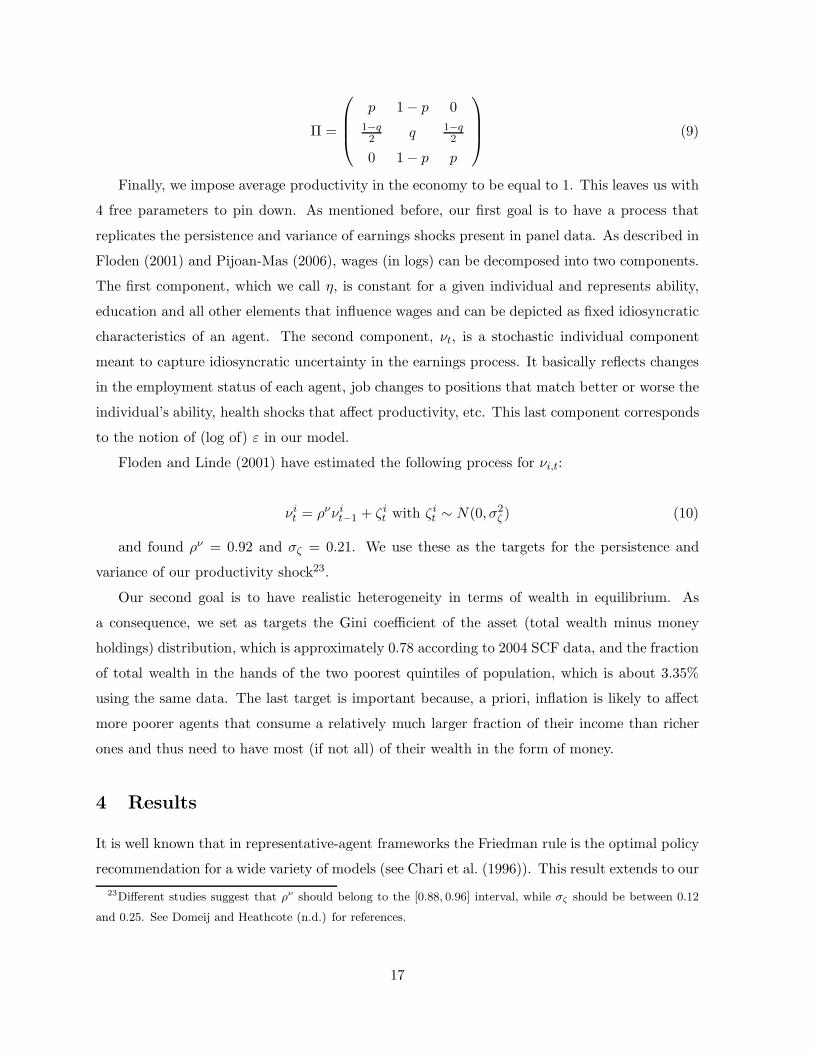
Π =

p 1 − p 0

1−q2

q 1−q2

0 1 − p p

(9)

Finally, we impose average productivity in the economy to be equal to 1. This leaves us with

4 free parameters to pin down. As mentioned before, our first goal is to have a process that

replicates the persistence and variance of earnings shocks present in panel data. As described in

Floden (2001) and Pijoan-Mas (2006), wages (in logs) can be decomposed into two components.

The first component, which we call η, is constant for a given individual and represents ability,

education and all other elements that influence wages and can be depicted as fixed idiosyncratic

characteristics of an agent. The second component, νt, is a stochastic individual component

meant to capture idiosyncratic uncertainty in the earnings process. It basically reflects changes

in the employment status of each agent, job changes to positions that match better or worse the

individual’s ability, health shocks that affect productivity, etc. This last component corresponds

to the notion of (log of) ε in our model.

Floden and Linde (2001) have estimated the following process for νi,t:

νit = ρννi

t−1 + ζit with ζi

t ∼ N(0, σ2ζ ) (10)

and found ρν = 0.92 and σζ = 0.21. We use these as the targets for the persistence and

variance of our productivity shock23.

Our second goal is to have realistic heterogeneity in terms of wealth in equilibrium. As

a consequence, we set as targets the Gini coefficient of the asset (total wealth minus money

holdings) distribution, which is approximately 0.78 according to 2004 SCF data, and the fraction

of total wealth in the hands of the two poorest quintiles of population, which is about 3.35%

using the same data. The last target is important because, a priori, inflation is likely to affect

more poorer agents that consume a relatively much larger fraction of their income than richer

ones and thus need to have most (if not all) of their wealth in the form of money.

4 Results

It is well known that in representative-agent frameworks the Friedman rule is the optimal policy

recommendation for a wide variety of models (see Chari et al. (1996)). This result extends to our

23Different studies suggest that ρν should belong to the [0.88, 0.96] interval, while σζ should be between 0.12

and 0.25. See Domeij and Heathcote (n.d.) for references.

17

model economy if we shut down heterogeneity among households. In the case in which εit = ε ∀i

a benevolent planner sets R = 1. The intuition behind this result lies in the uniform commodity

taxation argument from the public finance literature. Notice that in our framework goods bought

with cash and with credit enter the utility function in identical manner24. Therefore, the tax

on labor income implicitly taxes all goods, whether bought with cash or with an alternative

transaction technology, at an identical rate. Setting R > 1 entails taxing more those goods

bought with cash, which is not efficient. Given the representative-agent assumption, in the

model we are describing there are no issues of redistribution or self-insurance. Moreover, the

capital-labor ratio is pinned down by the intertemporal discount factor β, so inflation does not

affect the return on capital or the wage rate. Thus, efficiency in the taxation of different goods

is the only aspect that the planner should take into account when designing the optimal policy

plan.

When we introduce idiosyncratic uninsurable risk the analysis changes substantially. Now

inflation has effects over the level of capital in steady state. In addition, due to the presence of

an alternative transaction technology like the one have introduced, inflation acts as a regressive

tax on consumption. We proceed to describe these effects in detail. We argue that, once these

effects are taken into consideration, the determination of the optimal policy mix remains an

open question that needs a quantitative answer.

4.1 Inflation as a regressive tax on consumption

As described by Erosa and Ventura (2002), inflation can act as a regressive consumption tax

when, in a heterogeneous agent setup such as ours, we allow agents to substitute cash by an

alternative transaction technology that displays economies of scale. For the moment we abstract

from the presence of idiosyncratic risk, since all the analysis holds by allowing for heterogeneity

in labor productivities only.

Without loss of generality, assume that an agent’s productivity εi is constant ∀t, εi ∈ E =

[ε1, ε2] with ε1 < ε2 and there is an equal mass of each type of agent in the population 25.

Furthermore, assume for simplicity that the initial wealth holdings w10 and w2

0 are such that the

economy is in steady state from t = 0 onwards. Then, optimality for agent i requires that

24The argument that follows holds always that utility is separable in consumption and leisure, and the utility

over consumption goods is homothetic, see Chari et al. (1996) for a formal proof in a similar model.25The results of this section are robust to changes in the number of productivity states and in the composition

of the population.

18

R = 1 +ωγ(zi)

ci(11)

The second term on the right hand side of the previous expression is the unitary cost of credit

for the threshold good zi. It is clear from expression (11) and from the functional specification

of the transaction technology (8) that this unitary cost decreases when the volume transacted

increases. Thus, the transaction technology displays economies of scale.

Assume for now that zi = 0 for i = 1, 2. From (11) it is immediate to see that z1 = z2 = 0

when R = 1, i.e, when the planner follows the Friedman rule both types of agents buy all

consumption goods using cash, since holding cash does not bring about any opportunity cost.

On the contrary, if R > 1, z2 > z1 > 0, given that c2 > c1 because agent 2 enjoys a higher labor

income and, therefore, a higher level of consumption26. Then it follows that the more productive

agents use the credit technology more intensely. This feature of the model is consistent with the

evidence on transaction patterns and portfolio holdings that Erosa and Ventura (2002) report

in their paper, which can be summarized in three main facts: high income individuals buy a

smaller fraction of their consumption with cash, the fraction of wealth in the form of liquid assets

held by a household decreases with her wealth and income and, finally, a fraction of households

does not own a credit card.

Due to the presence of economies of scale in the transaction technology, buying goods with

credit is relatively more expensive for less productive agents. Because these agents buy a larger

fraction of goods with cash, they need to hold a relatively larger fraction of their income in liquid

assets. It is in this sense that inflation acts as a regressive tax on consumption, since setting

R > 1 corresponds to taxing more low-income individuals.

If z2 > z1 this asymmetric effect of the inflation tax is exacerbated. As we discussed in section

2.2.2, the introduction of zi is a shortcut to model differences in the access to commercial credit

markets that high-income, rich households enjoy when compared to poor, low-income ones. The

regressive nature of the inflation tax implies that for high productivity households it is optimal

to set a gross nominal interest rate higher than 1, since in this way the burden of taxation is

shifted to poor, unproductive individuals. To see the intuition behind this statement, think of

the limit case in which z2 = 1. In this case the inflation tax does not affect agents of type 2 in

any way, so they would want the government to set it as high as necessary to finance completely

its expenditure from seigniorage revenue.

In the appendix we show (numerically) that, in the current setup, a benevolent government

26Strictly speaking, this is only true for particular levels of initial wealth w1

0 and w2

0 . Here we are implicitly

making the assumption that the more productive agent is at least as rich as the less productive one.

19

(a Ramsey planner) that assigns a sufficiently high Pareto weight on type 2 agents would find

it optimal to deviate from the Friedman rule and set R > 1.

4.2 Inflation as a motive for precautionary savings

The effect described in the previous section is at work due to the assumption of heterogeneity

and the transaction technology we have specified, but it does not depend on the presence of

uninsurable idiosyncratic risk. In this section we argue that inflation accentuates such risk and

that, consequently, households save more when inflation is high.

Consider first the case in which there is no uncertainty (aggregate or idiosyncratic). Then

the capital/labor ratio is determined in steady state by the discount factor β and is completely

independent of the inflation rate. In this sense inflation is neutral and it does not affect the

wage rate or the real interest rate in steady state. This is also true if we allow for idiosyncratic

uncertainty but assume that households can trade a complete set of Arrow securities contingent

on the realization of the labor productivity shock. It is easy to show that in this case agents

can do full risk sharing and, if there is no aggregate uncertainty and utility is separable in

consumption and leisure, enjoy a constant level of consumption independently of their current

labor productivity. As in the case with no uncertainty, β determines the aggregate capital-labor

ratio, ω and r27.

In models with incomplete markets and borrowing constraints, agents save not only to smooth

consumption by transferring resources from one period to the other, but also to insure themselves

against bad realizations of the shock that may push them close to the borrowing constraint

and force them to consume very little. The absence of complete markets and the presence

of borrowing constraints lead agents to save for precautionary reasons28. Moreover, the more

uncertain future income (and consumption) becomes, the stronger the motive for precautionary

savings. The increase in savings translates into an increase in the capital stock in steady state,

with the consequent decrease in the real interest rate and increase in the wage rate.

In the economy we have described, a higher level of steady state inflation implies that future

consumption is more uncertain and, consequently, reinforces the incentives to save. To see this,

consider the no-borrowing constraint of household i, which says that Ait ≥ 0. As shown in the

appendix, this constraint can be re-written as:

27We have abstracted from the possibility that there is aggregate uncertainty. In this case, if there are incomplete

markets with respect to the aggregate shock, inflation can have an active role as a mechanism to complete the

markets. See Chari et al. (1991) for a discussion.28When the marginal utility is convex, i.e., utility displays a positive third derivative and, independently of the

presence of borrowing constraints, agents save because of prudence.

20

cit(1 − zit)(1 + π) ≤ wi

t (12)

where π is the inflation rate. Consider a steady state with πA, in which household i at time

t hits the constraint:

ci,At (1 − zi,At )(1 + πA) = wi,A

t

If inflation were higher, say πB > πA, to sustain the same level of consumption ci,At and the

same fraction of goods bought with credit zi,A, household i would need to have a higher level of

wealth in order to satisfy constraint (12). Similarly, for a household i that has wealth holdings

wi,At in an economy where the inflation rate is πB > πA, either ci,Bt < ci,At , zi,B

t > zi,At , or a

combination of both. Raising zit entails working more to be able to pay for the higher credit

expenses; since the intratemporal optimality condition (23) has to be satisfied, consumption

needs to decrease, so it has to be the case that ci,Bt < ci,At . This means that the higher level of

inflation πB renders consumption more uncertain.

The previous discussion points out to the fact that inflation raises the incentives to save

and, as a consequence, the level of steady- state capital. Thus, an economy with higher inflation

displays a lower real interest rate and higher wages. Also, because the budget constraint of

the government (5) has to be satisfied, the higher seigniorage revenue calls for a decrease in

τ l. Poor agents, who rely almost entirely on their labor income and whose marginal utilities of

consumption and leisure are very large, find this beneficial because a small increase in disposable

income translates into a sizeable increase in utility. On the other hand, middle-class and rich

households are harmed by the reduction in their capital income derived from the lower real

interest rate.

4.3 Optimal policy

In the previous two sections we have discussed the role that the inflation tax has as a regressive

tax on consumption and as an incentive for capital accumulation. The two effects affect asym-

metrically different sectors of the population: while the former benefits richer, more productive

agents, the latter increases welfare of the poor, unproductive ones.

Having exposed all the mechanisms by which inflation affects the agents in our economy,

it should be clear by now that the determination of the optimal policy mix is a question that

does not have an immediate answer. There are a variety of effects operating simultaneously,

affecting different agents in contradictory ways. The only way to provide an answer is to find

the optimum policy numerically, once we have a reasonably calibrated model economy.

21

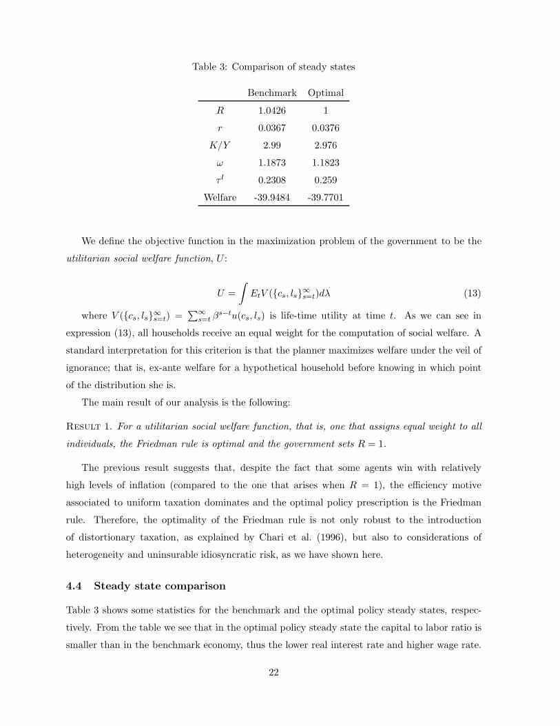
Table 3: Comparison of steady states

Benchmark Optimal

R 1.0426 1

r 0.0367 0.0376

K/Y 2.99 2.976

ω 1.1873 1.1823

τ l 0.2308 0.259

Welfare -39.9484 -39.7701

We define the objective function in the maximization problem of the government to be the

utilitarian social welfare function, U :

U =

∫

EtV ({cs, ls}∞s=t)dλ (13)

where V ({cs, ls}∞s=t) =

∑∞s=t β

s−tu(cs, ls) is life-time utility at time t. As we can see in

expression (13), all households receive an equal weight for the computation of social welfare. A

standard interpretation for this criterion is that the planner maximizes welfare under the veil of

ignorance; that is, ex-ante welfare for a hypothetical household before knowing in which point

of the distribution she is.

The main result of our analysis is the following:

Result 1. For a utilitarian social welfare function, that is, one that assigns equal weight to all

individuals, the Friedman rule is optimal and the government sets R = 1.

The previous result suggests that, despite the fact that some agents win with relatively

high levels of inflation (compared to the one that arises when R = 1), the efficiency motive

associated to uniform taxation dominates and the optimal policy prescription is the Friedman

rule. Therefore, the optimality of the Friedman rule is not only robust to the introduction

of distortionary taxation, as explained by Chari et al. (1996), but also to considerations of

heterogeneity and uninsurable idiosyncratic risk, as we have shown here.

4.4 Steady state comparison

Table 3 shows some statistics for the benchmark and the optimal policy steady states, respec-

tively. From the table we see that in the optimal policy steady state the capital to labor ratio is

smaller than in the benchmark economy, thus the lower real interest rate and higher wage rate.

22

0 5 10 15 20 250

0.2

0.4

0.6

0.8

1

1.2

1.4

Wealth

Con

sum

ptio

n (ε

1 )

0 5 10 15 20 250.2

0.4

0.6

0.8

1

1.2

1.4

1.6

Wealth

Con

sum

ptio

n (ε

2 )

0 5 10 15 20 250.8

0.9

1

1.1

1.2

1.3

1.4

1.5

1.6

1.7

1.8

Wealth

Con

sum

ptio

n (ε

3 )

BenchmarkOptimal

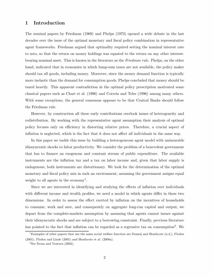
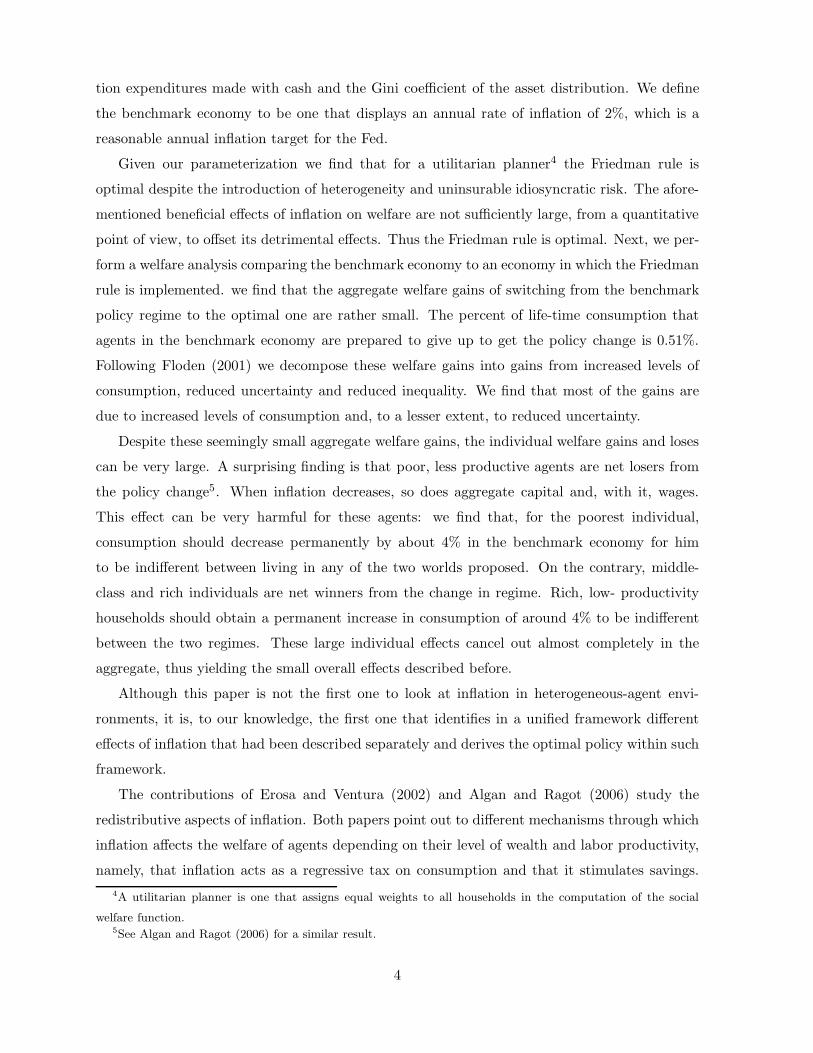
Figure 2: Consumption

This is a direct consequence of the fact that inflation reinforces the motive for precautionary

savings, as discussed in the previous section. The lower wage, lower savings and lower seignior-

age revenue force the government to increase the tax rate on labor income in order to balance

its budget. Therefore τ l is higher in the optimal policy economy.

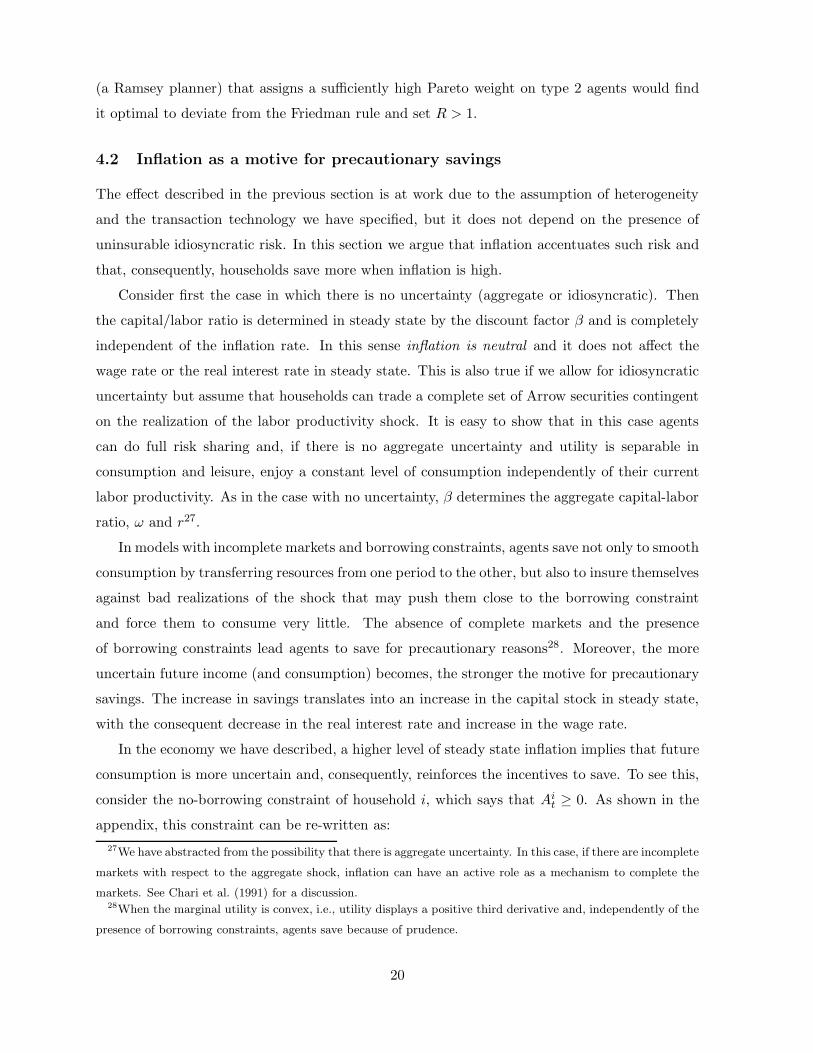
Figures 2 and 3 shows consumption and leisure policy functions in the benchmark economy

and in the optimal policy one, for the three levels of labor productivity. It can be observed

that, for ε1 and ε2 and very low levels of wealth, consumption and leisure are higher in the

benchmark economy, the reason being the higher labor income that poor households enjoy.

When wealth increases the return on capital holdings starts being a relevant source of income for

the household. Since the real interest rate is lower in the benchmark economy, consumption and

leisure decrease. For high productivity households the picture looks different. These households

are always enjoying a high level of consumption, and even for very little levels of wealth their

labor income is sufficiently high to finance high consumption and savings. The decrease in

uncertainty as a consequence of lower inflation levels present in the optimal policy economy

diminish the incentives to save for precautionary reasons. Therefore, very productive agents can

afford to work less and enjoy higher levels of leisure, even if this means giving up some of their

consumption.

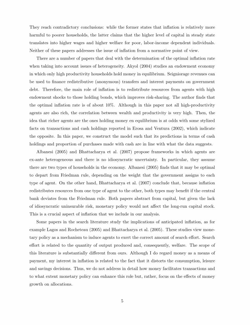
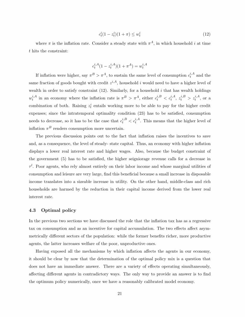
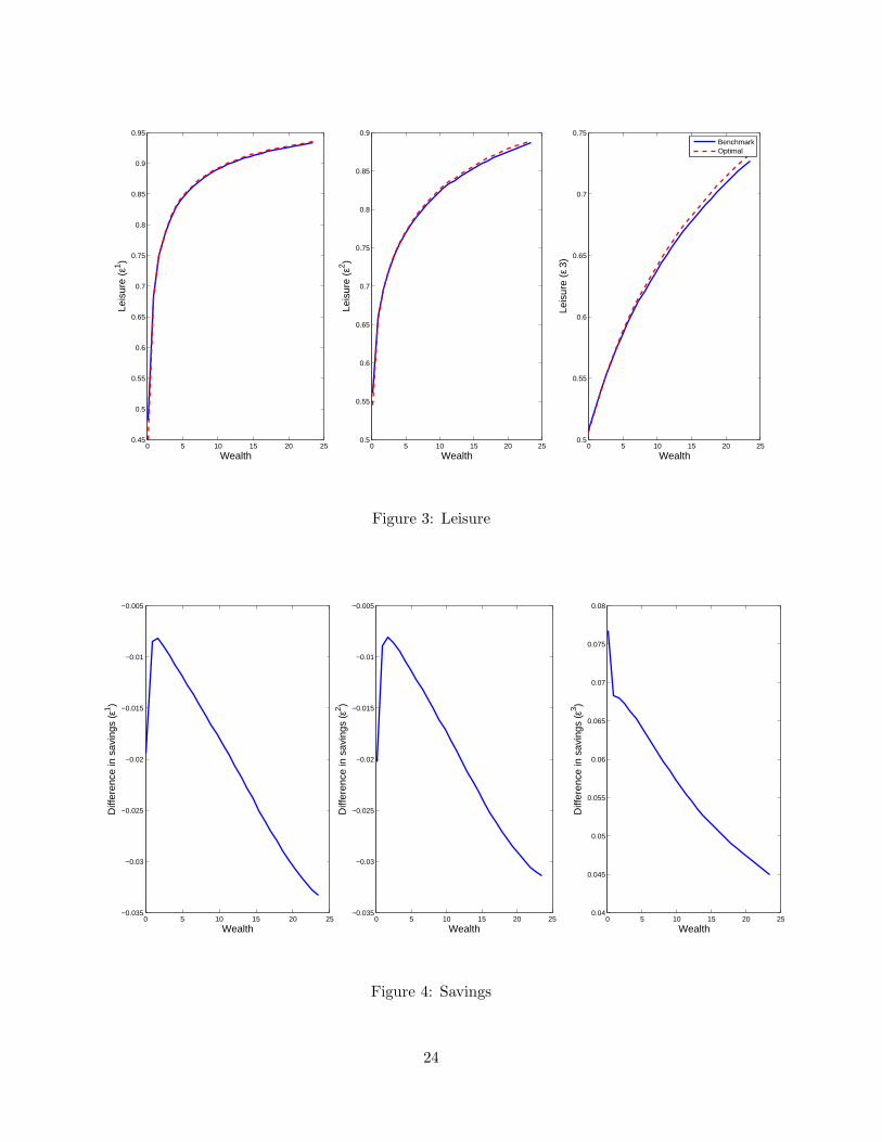
Figure 4 plots the difference in savings between the benchmark economy and the optimal

23

0 5 10 15 20 250.45

0.5

0.55

0.6

0.65

0.7

0.75

0.8

0.85

0.9

0.95

Wealth

Leis

ure

(ε1 )

0 5 10 15 20 250.5

0.55

0.6

0.65

0.7

0.75

0.8

0.85

0.9

Wealth

Leis

ure

(ε2 )

0 5 10 15 20 250.5

0.55

0.6

0.65

0.7

0.75

Wealth

Leis

ure

(ε 3)

BenchmarkOptimal

Figure 3: Leisure

0 5 10 15 20 25−0.035

−0.03

−0.025

−0.02

−0.015

−0.01

−0.005

Wealth

Diff

eren

ce in

sav

ings

(ε1 )

0 5 10 15 20 25−0.035

−0.03

−0.025

−0.02

−0.015

−0.01

−0.005

Wealth

Diff

eren

ce in

sav

ings

(ε2 )

0 5 10 15 20 250.04

0.045

0.05

0.055

0.06

0.065

0.07

0.075

0.08

Wealth

Diff

eren

ce in

sav

ings

(ε3 )

Figure 4: Savings

24

0 5 10 15 20 250

0.1

0.2

0.3

0.4

0.5

0.6

0.7

0.8

0.9

1

Wealth

Zi

ε1

ε2

ε3

Figure 5: Transaction technology use

policy one. It is immediate to see that, for agents with ε1 and ε2, this difference is always

negative, thus savings are higher in the optimal policy steady state. For agents with ε3, however,

the contrary statement is true. Again, this result hinges on the fact that high productivity

agents need to save less for self-insurance reasons when R = 1. Agents with low and medium

productivity and very little wealth need to save more because hitting the constraint is more

harmful in this case. Notice that this is the reason why the curve of the difference in savings

first rises and then goes down. As wealth increases, their total income goes up and they are able

to better self-insure by saving more.

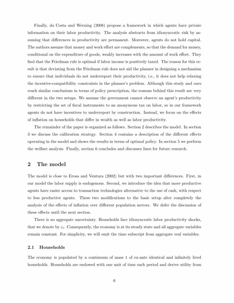
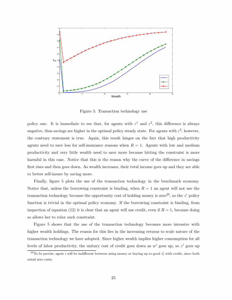
Finally, figure 5 plots the use of the transaction technology in the benchmark economy.

Notice that, unless the borrowing constraint is binding, when R = 1 an agent will not use the

transaction technology because the opportunity cost of holding money is zero29, so the zi policy

function is trivial in the optimal policy economy. If the borrowing constraint is binding, from

inspection of equation (12) it is clear that an agent will use credit, even if R = 1, because doing

so allows her to relax such constraint.

Figure 5 shows that the use of the transaction technology becomes more intensive with

higher wealth holdings. The reason for this lies in the increasing returns to scale nature of the

transaction technology we have adopted. Since higher wealth implies higher consumption for all

levels of labor productivity, the unitary cost of credit goes down as wi goes up, so zi goes up

29To be precise, agent i will be indifferent between using money or buying up to good zit with credit, since both

entail zero costs.

25

as well. Increasing returns to scale are also responsible for the three lines, corresponding to the

three labor productivity levels, becoming closer together as wealth increases, since for high wi

the differences in consumption become smaller.

5 Welfare analysis

We proceed to compare aggregate welfare in the benchmark economy (with a level of inflation of

2% annually) and in the economy in which the optimal policy is implemented. In this section we

are comparing welfare in two different steady states, and we are not saying anything as to what

happens during the transition from one to the other if there is a reform on policy. Obviously,

studying the transition is a very interesting exercise, specially if we want to determine the

“optimal transition”, i.e., the transition such that no agent loses from the policy reform. As

shown by Greulich and Marcet (2008) the optimal transition can imply a policy during the

transition very different from the long-run policy prescription. We leave the analysis of the

transition for future research.

We need to start with some definitions. The overall utilitarian welfare gain of the policy

gain, U is such that

∫

EtV ({(1 +U )cBs , lBs }∞s=t)dλ

B =

∫

EtV ({cOs , lOs }

∞s=t)dλ

O

where the superscript B stands for the benchmark economy and O for the economy with the

optimal policy. U can be thought of as the percent permanent change in consumption that

agents in economy B should receive to be indifferent between living in economy B or in economy

O.

Notice that the utilitarian social welfare (eq. (13)) can increase for three reasons. The

first is when consumption or leisure increase for all agents. This is called the level effect. The

second, called inequality effect, is when inequality is reduced, since u(·) (and therefore V (·)) is

concave. Finally, since agents are risk-averse, if uncertainty is reduced U increases. This is the

uncertainty effect. Following Floden (2001), we can decompose the utilitarian welfare gain into

the welfare gains associated to the three effects mentioned before. In order to do this, define the

certainty-equivalent consumption bundle c as:

V ({c, ls}∞s=t) = EtV ({cs, ls}

∞s=t)

Call C =∫

cdλ, Leis =∫

ldλ and C =∫

cdλ average consumption, leisure and certainty-

equivalent consumption, respectively. Then the cost of uncertainty punc can be defined as

26

Table 4: Welfare gains

U = 0.0051 lev = 0.0044 unc = 0.0015 ine = −0.00005

V ({(1 − punc)C,Leis}∞s=t) = V ({C, Leis}∞s=t)

This is the fraction of average consumption that an individual with average consumption

and leisure would be willing to give up to avoid all the risk from labor productivity fluctua-

tions. When uncertainty increases, C decreases and, since C and Leis remain unchanged, punc

necessarily goes up.

Define the cost of inequality pine as

V ({(1 − pine)C, Leis}∞s=t) =

∫

V ({c, ls}∞s=t)dλ

If we redistribute consumption from a rich household to a poor one, C and Leis remain

unchanged. However, the right-hand side of the previous expression increases, so pine has to go

down. Finally, define leisure-compensated consumption in economy O, CO as

V ({CO, LeisB}∞s=t) = V ({CO, LeisO}∞s=t)

which is the average consumption level that would make life-time utility in economy O equal

to the one in an economy with the average leisure of economy B.

We are now ready to define the welfare gains associated to each one of the effects described

before:

• The welfare gain of increased levels, lev is

lev =CO

CB− 1

• The welfare gain of reduced uncertainty is

unc =1 − pO

unc

1 − pBunc

− 1

• The welfare gain of reduced inequality is

ine =1 − pO

ine

1 − pBine

− 1

27

ε1

ε2

ε3

0 5 10 15 20 25 30 35−0.04

−0.03

−0.02

−0.01

0

0.01

0.02

0.03

0.04

Wealth

Figure 6: Individual welfare gains

Table 4 shows the welfare gains in our setup. As we can see, the aggregate utilitarian welfare

gains are very small, only 0.51% of life-time consumption. The majority of these gains are due

to the change in consumption levels (0.44% of consumption), and the remaining is because of

the decrease in uncertainty that is associated with the optimal policy (0.15% of consumption).

The welfare gains associated to the decrease in inequality are, actually, welfare costs, and are

negligible.

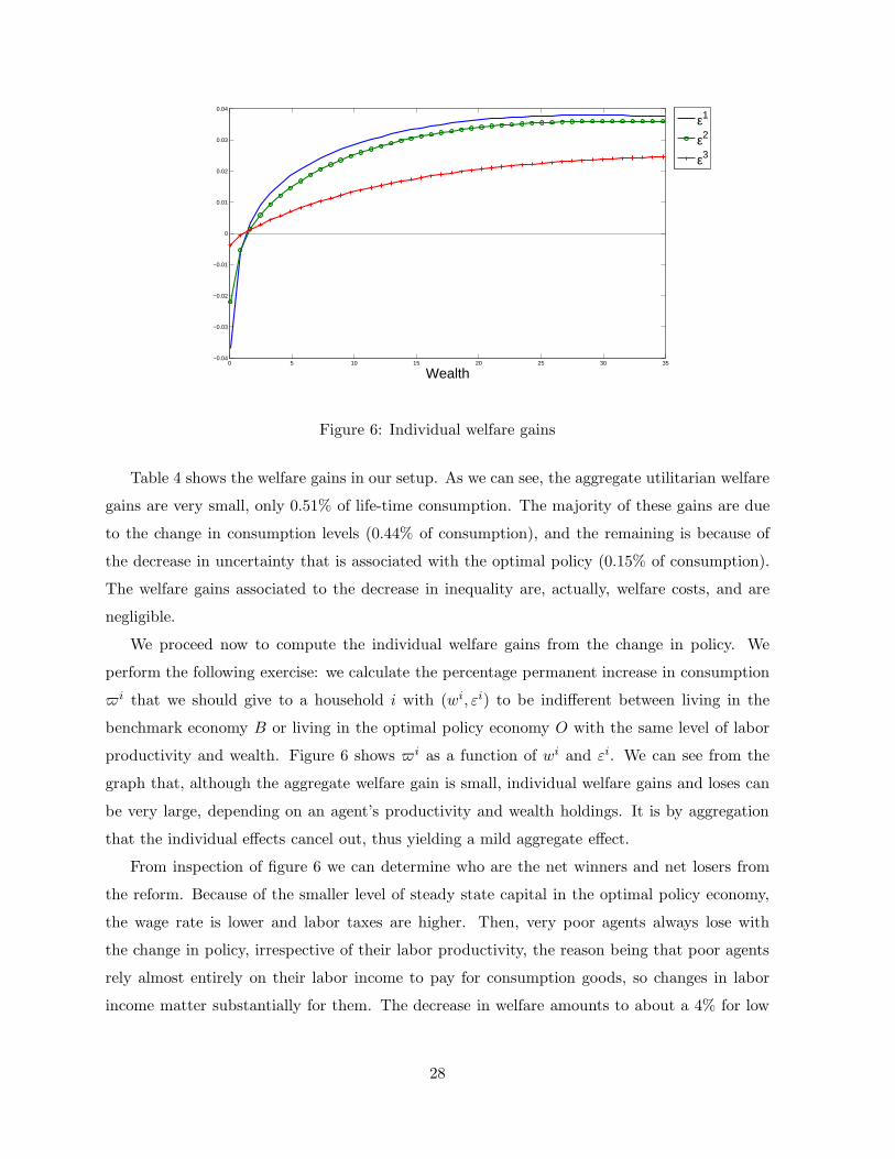
We proceed now to compute the individual welfare gains from the change in policy. We

perform the following exercise: we calculate the percentage permanent increase in consumption

i that we should give to a household i with (wi, εi) to be indifferent between living in the

benchmark economy B or living in the optimal policy economy O with the same level of labor

productivity and wealth. Figure 6 shows i as a function of wi and εi. We can see from the

graph that, although the aggregate welfare gain is small, individual welfare gains and loses can

be very large, depending on an agent’s productivity and wealth holdings. It is by aggregation

that the individual effects cancel out, thus yielding a mild aggregate effect.

From inspection of figure 6 we can determine who are the net winners and net losers from

the reform. Because of the smaller level of steady state capital in the optimal policy economy,

the wage rate is lower and labor taxes are higher. Then, very poor agents always lose with

the change in policy, irrespective of their labor productivity, the reason being that poor agents

rely almost entirely on their labor income to pay for consumption goods, so changes in labor

income matter substantially for them. The decrease in welfare amounts to about a 4% for low

28

productivity agents, while it is less than 1% for high productivity households. The difference

in these effects relies on the fact that utility is concave and agents with high ε are income-

rich, so they can afford higher levels of consumption and leisure. On the contrary, net winners

from the policy change are middle-class and rich households, again irrespective of their labor

productivity, who see their returns on capital increased because of the higher real interest rate.

Again, because of the concavity of the utility function, rich and low-productivity agents are the

ones that benefit the more. Their increase in welfare can reach a maximum of around 4%, while

for high-productivity households the maximum is about 2.5%.

6 Conclusions

The determination of the optimal monetary policy prescription in the long run is a crucial issue

for policy makers as well as for academics. Arguably, central banks set their inflation targets

according to some criteria related to the maximization of social welfare. The natural question

that arises is what the long-run optimal inflation target should be.

The standard literature in optimal monetary and fiscal policy, by focusing on representa-

tive agent environments, looks into this problem in a partial way and only considers issues of

efficiency in distributing the distortions associated to taxation. In this paper we have relaxed

the representative-agent assumption by allowing for heterogeneity and uninsurable idiosyncratic

risk. This allows us to include in the analysis issues of redistribution of the tax burden and

long-run effects of different tax schemes over capital and output that cannot be addressed in the

traditional framework.

We make the standard modeling assumption that agents demand cash because it provides

liquidity services. Moreover, we allow them to use an alternative costly transaction technology

by which they economize on their money holdings. This transaction technology reconciles the

model with some stylized facts reported in the literature regarding transaction patterns for

different sectors of population. We are able to identify the effects of inflation as a regressive tax

on consumption and as a motive to increase savings for precautionary reasons.

We calibrate the model to the U.S. economy and find that the optimal policy prescription

that arises from the exercise is the Friedman rule. This result provides robustness to what is a

classical result in representative-agent models. A surprising implication of the analysis is that,

despite the fact that inflation taxes relatively more consumption of poor agents, these agents

actually win with inflation, while middle-class and rich agents lose. Therefore, this analysis

challenges the conventional wisdom that inflation hurts the poor and benefits the rich.

29

The analysis presented here opens many avenues for future research. Probably one of the

most natural extensions is the study of the transition between the steady state with the bench-

mark policy and the one in which the optimal policy is implemented. Studying the transition

allows to perform a more accurate analysis of the welfare gains from the change in policy for

different individuals. Moreover, studying the optimal transition, i.e., the transition taking into

account that all agents should benefit from the reform, can lead to policy plans very different

than what is optimal in the long run, as in shown in Greulich and Marcet (2008).

On a related note, Doepke and Schneider (2006) have driven attention to the fact that

unexpected inflation can have large redistributive effects for individuals with different portfolio

holdings. As a further step, we would like to introduce aggregate fluctuations to a framework

similar in spirit to the one we consider here, but taking into account this heterogeneity of

portfolio holdings among different individuals. This type of environment is suitable for studying

optimal monetary and fiscal policy as stabilizing mechanisms for macroeconomic fluctuations,

an issue that has not been addressed in this paper.

30

References

Akyol, A.: 2004, Optimal monetary policy in an economy with incomplete markets and idiosyn-

cratic risk, Journal of Monetary Economics 51, 1245–1269.

Albanesi, S.: 2005, Optimal and time consistent monetary and fiscal policy with heterogeneous

agents, mimeo.

Algan, Y. and Ragot, X.: 2006, On the non-neutrality of money with borrowing constraints,

mimeo.

Bhattacharya, J., Haslag, J. and Martin, A.: 2005, Heterogeneity, redistribution and the Fried-

man rule, International Economic Review 46, 437–454.

Bhattacharya, J., Haslag, J., Martin, A. and Singh, R.: 2007, Who is afraid of the Friedman

rule?, Economic Inquiry 46, 113–130.

Campanale, C.: 2007, Increasing return to savings and wealth inequality, Review of Economic

Dynamics 10, 646–675.

Castaneda, A., Diaz-Gimenez, J. and Rios-Rull, J.: 2003, Accounting for the U.S. Earnings and

Wealth Inequality, Journal of Political Economy 111(4), 818–857.

Chari, V. V., Christiano, J. and Kehoe, P. J.: 1991, Optimal fiscal and monetary policy: some

recent results, Journal of Money, Credit and Banking 23, 519–539.

Chari, V. V., Christiano, J. and Kehoe, P. J.: 1996, Optimality of the Friedman rule in economies

with distorting taxes, Journal of Monetary Economics 37, 203–223.

Conesa, J. C. and Krueger, D.: 1999, Social security reform with heterogeneous agents, Review

of Economic Dynamics 2, 757–795.

Correia, I. and Teles, P.: 1996, Is the Friedman rule optimal when money is an intermediate

good?, Journal of Monetary Economics 38, 223–244.

da Costa, C. and Werning, I.: 2008, On the optimality of the friedman rule with heterogeneous

agents and non-linear income taxation, Journal of Political Economy 116.

Doepke, M. and Schneider, M.: 2006, Inflation and the redistribution of nominal wealth, Journal

of Political Economy 114, 1069–1097.

31

Domeij, D. and Floden, M.: 2006, The labor supply elasticity and borrowing constraints: why

estimates are biased, Review of Economic Dynamics 9, 242–262.

Domeij, D. and Heathcote, J.: n.d., On the distributional effects of reducing capital taxes,

International Economic Review .

Dotsey, M. and Ireland, P.: 1996, The welfare cost of inflation in general equilibrium, Journal

of Monetary Economics 37, 29–47.

Erosa, A. and Ventura, G.: 2002, On inflation as a regressive consumption tax, Journal of

Monetary Economics 49, 761–795.

Floden, M.: 2001, The effectiveness of government debt and transfers as insurance, Journal of

Monetary Economics 48, 81–108.

Floden, M. and Linde, J.: 2001, Idisyncratic Risk in the U.S. and Sweden: Is there a Role for

Government Insurance?, Review of Economic Dynamics 4, 406–437.

Friedman, M.: 1969, The optimum quantity of money, The optimum quantity of money and

other essays pp. 1–50.

Greulich, K. and Marcet, A.: 2008, Pareto-improving optimal capital and labor taxes, mimeo.

Heathcote, J., Storesletten, K. and Violante, G.: 2008a, Insurance and opportunities: A welfare

analysis of labor market risk, Journal of Monetary Economics 55, 501–525.

Heathcote, J., Storesletten, K. and Violante, G.: 2008b, The macroeconomic implications of

rising wage intequality in the United States, Working paper, NBER.

Lagos, R. and Rocheteau, G.: 2005, Inflation, output and welfare, International Economic

Review 46, 495–522.

Lucas, R. E. and Stokey, N. L.: 1983, Optimal fiscal and monetary policy in an economy without

capital, Journal of Monetary Economics 12, 55–93.

Phelps, E.: 1973, Inflation in the theory of public finance, Swedish Journal of Economics 75, 67–

82.

Pijoan-Mas, J.: 2006, Precautionary savings or working longer hours?, Review of Economic

Dynamics 9, 326–352.

32

A Appendix

A.1 Optimality conditions of the household

The problem of household i is

max E0

∞∑

t=0

βtu(cit, lit) (14)

subject to

ptcit + qt

∫ zit

0

γi(j)dj +W it+1 = RAi

t +M it + (1 − τ l)ωpt(1 − lit)ε

it (15)

ptcit(1 − zi

t) ≤M it (16)

Ait ≥ 0 (17)

We define

at =At

pt−1

wt =Wt

pt−1

mt =Mt

pt−1

We can rewrite equations (15) and (16) in real terms by diving both sides of the equations

by pt:

cit + q + ω

∫ zit

0

γi(j)dj + wit+1 = (1 + r)ai

t +mi

t

1 + Π+ (1 − τ l)ω(1 − lit)ε

it (18)

cit(1 − zit) ≤

mit

1 + Π=mi

tR

1 + r(19)

where we have used the fact that pt

pt−1= 1+Π, qt = ωpt and R = (1+ r)(1+Π). r = r(1−τk)

is the after-tax real return on capital.

Plugging equation (19) into (18), using wit = ai

t +mit and rearranging, we obtain

33

cit(1 − (1 − zit)(1 −R)) + q + ω

∫ zit

0

γi(j)dj + wit+1 = (1 + r)wi

t + (1 − τ l)ω(1 − lit)εit (20)

Similarly, equation (17) can be rewritten as

cit(1 − zit)

R

1 + r− wi

t ≤ 0 (21)

The problem of the household becomes maximizing (14) subject to constraints (20) and (21).

The optimality conditions of the household are:

R = 1 +ωγ(zi

t)

cit(22)

ul,t

εituc,t

Γt = (1 − τ l)ω (23)

where

Γt =

(

1 + (1 − zit)ωγ(zi

t)

cit

)

along with the Euler equation. Call µt the multiplier associated to constraint (21). If the

borrowing constraint in period t + 1 is not binding, i.e., if µt+1 = 0, then the corresponding

Euler equation is

uc,t

Γt= β(1 + r)Et

uc,t+1

Γt+1

(24)

If, on the contrary, µt+1 > 0 the Euler equation becomes

uc,t

Γt= β(1 + r)Et

uc,t+1

Γt+1

(

1 +1

R

(

(1 −R) +ωγ(zi

t+1)

cit+1

))

(25)

Given that equation (21) can be binding in t and/or in t + 1, 4 possible cases need to be

considered when solving for the allocations of agent i:

• µt = 0 and µt+1 = 0. The relevant equations for obtaining the allocations are (22), (23),

(24) and the budget constraint (20).

• µt > 0 and µt+1 = 0. The relevant equations for obtaining the allocations are (21), (23),

(24) and the budget constraint (20).

• µt = 0 and µt+1 > 0. The relevant equations for obtaining the allocations are (22), (23),

(25) and the budget constraint (20).

34

• µt > 0 and µt+1 > 0. The relevant equations for obtaining the allocations are (21), (23),

(25) and the budget constraint (20).

A.2 Optimal fiscal and monetary policy with constant heterogeneity and no

idiosyncratic risk

As in section 4.1, assume that an agent’s productivity εi is constant ∀t, εi ∈ E = [ε1, ε2] with

ε1 < ε2 and there is an equal mass of each type of agent in the population 30. Furthermore,

assume for simplicity that the initial wealth holdings w10 and w2

0 are such that the economy is

in steady state from t = 0 onwards.

Consider the case of a benevolent government (a Ramsey planner) that has to decide on the

level of R and τ l in our economy, in order to maximize a social welfare function given by the

weighted sum of the utilities of both types of agents. The problem of the government can be

written as:

max{ci,li,zi}

∞∑

t=0

βtu(ci, li)

s.t.

1

1 − β

[

ucici +ucici

ci + (1 − zi)γ(zi)FLg

FLg

∫ zi

zi

γ(j)dj − uli(1 − li)

]

=ucici(1 + r)

ci + (1 − zi)γ(zi)FLg

W i−1 i = 1, 2

(26)

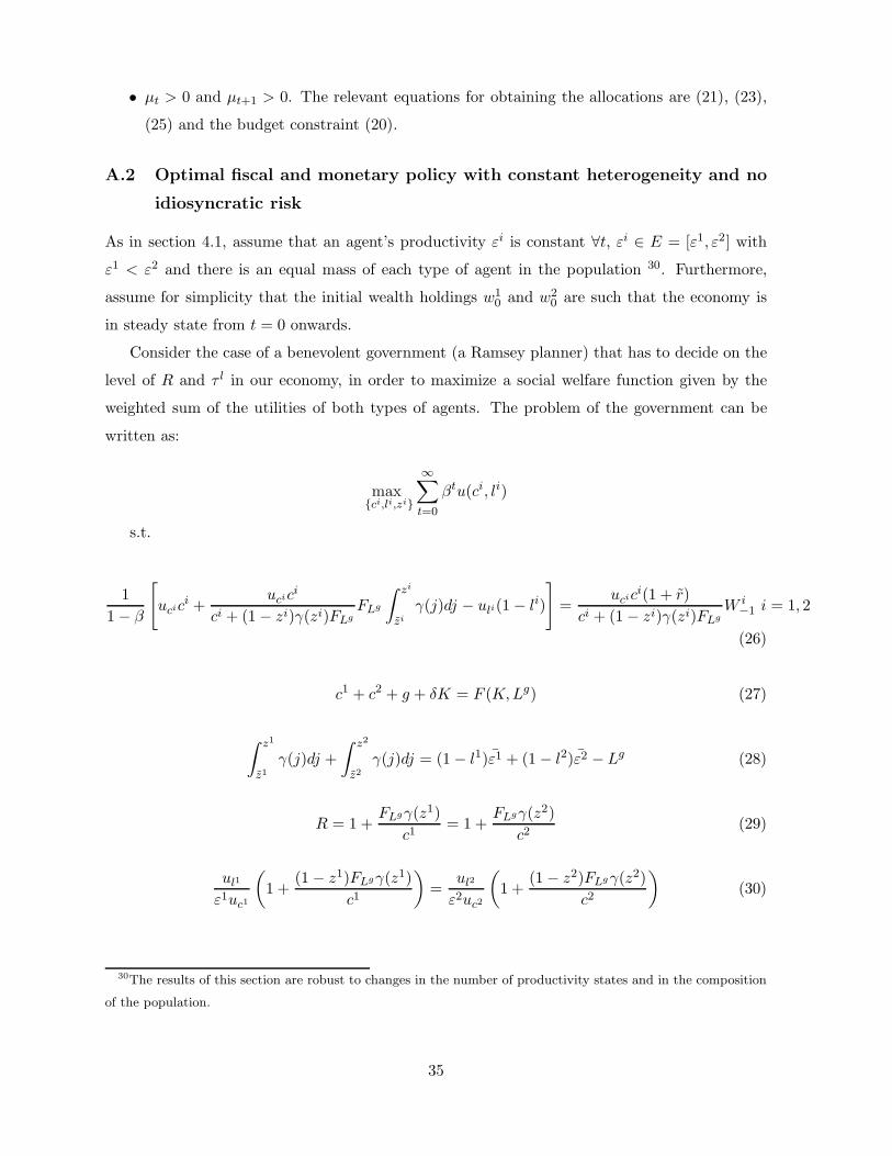
c1 + c2 + g + δK = F (K,Lg) (27)

∫ z1

z1

γ(j)dj +

∫ z2

z2

γ(j)dj = (1 − l1)ε1 + (1 − l2)ε2 − Lg (28)

R = 1 +FLgγ(z1)

c1= 1 +

FLgγ(z2)

c2(29)

ul1

ε1uc1

(

1 +(1 − z1)FLgγ(z1)

c1

)

=ul2

ε2uc2

(

1 +(1 − z2)FLgγ(z2)

c2

)

(30)

30The results of this section are robust to changes in the number of productivity states and in the composition

of the population.

35

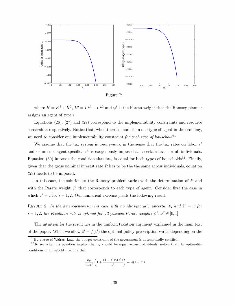
1 1.01 1.02 1.03 1.04 1.05 1.06 1.07−4.1965

−4.196

−4.1955

−4.195

−4.1945

−4.194

−4.1935

−4.193

R

Util

ity o

f age

nt ty

pe 1

1 1.01 1.02 1.03 1.04 1.05 1.06 1.07−2.1028

−2.1026

−2.1024

−2.1022

−2.102

−2.1018

−2.1016

−2.1014

−2.1012

R

Util

ity o

f age

nt ty

pe 2

Figure 7:

where K = K1 +K2, Lg = Lg,1 +Lg,2 and ψi is the Pareto weight that the Ramsey planner

assigns an agent of type i.

Equations (26), (27) and (28) correspond to the implementability constraints and resource

constraints respectively. Notice that, when there is more than one type of agent in the economy,

we need to consider one implementability constraint for each type of household31 .

We assume that the tax system is anonymous, in the sense that the tax rates on labor τ l

and τk are not agent-specific. τk is exogenously imposed at a certain level for all individuals.

Equation (30) imposes the condition that taul is equal for both types of households32. Finally,

given that the gross nominal interest rate R has to be the the same across individuals, equation

(29) needs to be imposed.

In this case, the solution to the Ramsey problem varies with the determination of zi and

with the Pareto weight ψi that corresponds to each type of agent. Consider first the case in

which zi = z for i = 1, 2. Our numerical exercise yields the following result:

Result 2. In the heterogeneous-agent case with no idiosyncratic uncertainty and zi = z for

i = 1, 2, the Friedman rule is optimal for all possible Pareto weights ψ1, ψ2 ∈ [0, 1].

The intuition for the result lies in the uniform taxation argument explained in the main text

of the paper. When we allow zi = f(εi) the optimal policy prescription varies depending on the

31By virtue of Walras’ Law, the budget constraint of the government is automatically satisfied.32To see why this equation implies that τl should be equal across individuals, notice that the optimality

conditions of household i require that

uli

uciεi

„

1 +(1 − zi)γ(zi)

ci

«

= ω(1 − τ l)

36

1 1.01 1.02 1.03 1.04 1.05−4.1985

−4.198

−4.1975

−4.197

−4.1965

−4.196

−4.1955

−4.195

−4.1945

−4.194

−4.1935

R

Util

ity o

f age

nt ty

pe 1

1 1.01 1.02 1.03 1.04 1.05−2.1022

−2.102

−2.1018

−2.1016

−2.1014

−2.1012

−2.101

R

Util

ity o

f age

nt ty

pe 2

Figure 8:

Pareto weights we consider, as summarized below:

Result 3. Assume zi = f(εi) and ∂zi

εi > 0, so that z1 < z2. Then, for a high enough Pareto

weight on the more productive agents, ψ2, the planner deviates from the Friedman rule and sets

R > 1.

Figures 7 and 8 illustrate what is stated in results 2 and 3. These figures show the utilities

of the two types of agents for R ∈ [1, 1.05] for the cases in which zi = 0 for i = 1, 2 and

z2 = 0.2 > z1 = 0, respectively. As we can see, in the first case the utility of both agents

is decreasing in R, while in the second case the utility of agents with ε2 is humped-shaped,

increasing first with R, reaching a maximum and then decreasing for higher values of the nominal

interest rate. The behavior of this utility causes the utility of the planner to be humped-shaped

as well, provided that the weight on agents with ε2 is high enough.

To grasp the intuition behind result 3, rewrite equation (23) as

uli

εiuci

=ω(1 − τ l)

1 + (1 − zi)(R− 1)(31)

Now assume that z2 is large, that ψ2 → 1 and ψ1 → 0. In this case the denominator of the

right hand side of expression (31) will be close to 1, even if R is very large. Since the planner

cares only about agent 2, it wants to distort as little as possible the intratemporal decision

of agent 2, therefore it wants the wedge between the marginal utility of leisure and that of

consumption to be as close to one as possible. From expression (31) it is clear that the way to

achieve this is to set τ l as low as possible while relying heavily on seigniorage revenues to finance

37

its budget. Since agents with ε2 can shelter from inflation by recurring to credit, this is clearly

optimal.

38