Seismic Data Reconstruction viaShearlet-Regularized Directional Inpainting

Soren Hauser∗ and Jianwei Ma†

May 15, 2012

We propose a new method for seismic data reconstruction by directional weightedshearlet-regularized image inpainting. The main idea is the application of a direc-tional and scale dependent thresholding (sdt) to penalize the vertical artifact edges.The alternating direction method of multipliers (ADMM) is used to solve the re-sulting sparsity-promoting `1-norm regularization. Numerical experiments show avery good performance of the proposed method.

1 Introduction

In applied geophysics various methods were developed to investigate the subsurface. Due to itsability to produce images down to depths of thousands of meters with a good resolution, theseismic method has become the most commonly used geophysical method in the oil and gasindustry. The simplest possible seismic measurement would be a 1D pint measurement with asingle source (often referred to as a shot) and receiver, both located in the same place. Theresults could be displayed as a seismic trace, which is a graph of the signal amplitude againsttravel time. Much more useful is a 2D measurement, with sources and receivers positionedalong a line on the surface. In practice, many receivers regularly spaced along the line are usedto record the signal from a series of source points. To avoid information losses, the seismicdata should be sampled according to the Shannon-Nyquist criterion. However, seismic dataare often sparsely or incompletely sampled along the spatial coordinates, partly caused bysurface obstacles, dead trace, no-permit areas and economic constraints. So the reconstructionand interpolation of seismic data is a very important problem in the seismic community. Thequality of reconstruction will impact the subsequent seismic processing steps, e.g., denoising,AVO, imaging, etc.

Many methods have been proposed for the reconstruction of seismic data. These methods aremainly divided into two categories: wave-equation methods and signal processing methods.The former methods use the simulation of wave propagation to reconstruct seismic data, so

∗Department of Mathematics, University of Kaiserslautern, Kaiserslautern, Germany,haeuser@mathematik.uni-kl.de

†Institute of Applied Mathematics, Harbin Institute of Technology, Harbin, China, jma@hit.edu.cn

1

that they require subsurface information (e.g., velocity distribution in earth medium), see e.g.[21, 26]. Most methods in the signal-processing-based category use sparse transforms such asthe Radon transform [13, 28], Fourier transform [22, 29, 17], and curvelet transform [11, 12,27, 18]. In particular, Herrmann et al. [11, 12, 27] applied the sparsity-promoting `1-normminimization of curvelet coefficients, that leads to much improved results for edge/lineups-preserving reconstruction. It is well known that the curvelet transform sparsely representsseismic data that mainly includes line-like features. Thanks to the theory of compressedsensing, the seismic data can be efficiently reconstructed after random down-sampling (ortaking less measurements) using a sparsity-promoting `1-norm convex optimization approach(even the sampling ratio is much less than the Shannon-Nyquist sampling ratio). This indicatesthat one can use less measured data (with more missing traces) to reconstruct the unknownseismic data with high precision. It could reduce the cost of seismic data survey.

The method in this paper also follows this line. Instead of the curvelet transform we use theshearlet transform introduced in [14] and described in its fully finite discrete form in [10] inthe sparsity-promoting `1-norm term. To our best knowledge this is the first time shearletsare used in the context of seismic data.

Another popular techniques is the use of prediction filters. For instance, the low-frequencynonaliased components or observed data are used to build antialiasing prediction-error filters,and then the filters are applied to interpolate high-frequency components or missing traces.The prediction-filter method can be implemented in t−x domain, f −x domain, even curveletdomain, e.g., [25, 20, 4, 15, 18, 18].

Recently, rank-reducing methods are used for the seismic data reconstruction. In [19], Oropezaand Sacchi reorganized the seismic data into a Hankel matrix, and then use multichannel sin-gular spectrum analysis (MSSA) to solve the rank-reduction problem of the Hankel matrix.In [31], Yang, Ma and Osher applied this theory and advanced fast algorithm of matrix com-pletion (MC) to seismic data reconstruction. Many existing fast algorithms of nuclear-normminimization can be applied in this framework. Recently, the authors [30] extended the low-rank method to a joint `1-norm of curvelet coefficient and nuclear-norm based low-rank methodfor seismic data reconstruction.

In this paper, our contribution is two-fold. We will describe the missing traces recovery as animage inpainting problem using shearlets in the `1-sparsity regularization term. The regular-ization parameter Λ is usually chosen only scale dependent (st). We propose the additionaluse of the directional information given by the shearlet coefficients (scale-directional, sdt). Inparticular we use different weights for the horizontal and for the vertical directions to reducevisible artifacts. This can be done efficiently using the simple data structure provided by therecently published Fast Finite Shearlet Transform (FFST) [10, 9].

The organization of the paper is as follows: In Section 2 we introduce the shearlet transform andthe basic steps for discretization. For our computations we will use FFST, an implementationof a translation invariant finite discrete shearlet transform discretized on the full grid. This isdifferent to other implementations, see, e.g., ShearLab [24]. In Section 3 we apply the convexinpainting model to the missing trace reconstruction problem and show how to incorporatethe shearlet transform into this model. We explain how the alternating direction methodof multipliers (ADMM) can be used to find the minimizer of the functional exploiting the

2

Parseval-frame property of the discrete shearlet transform. In the last Section 4 we presentthe numerical results for two different data sets.

2 Shearlets and Shearlet transform

In this first section we sketch the mathematical background of the shearlet transform that willbe used as part of our inpainting algorithm. Similar to curvelets [2] shearlets were developedto provide a directional multiscale decomposition of images. However, the rotation used forcurvelets to obtain the directional selectivity is replaced by a shear matrix Ss that reads

Ss =

(1 s0 1

), s ∈ R.

Note that the shearing is well suited for the discrete setting compared to the rotation used forthe curvelet transform. Additionally shearlets stem from a square-integrable group represen-tation, the so called shearlet group [5].

Similar to curvelets a shearlet is oriented in time (or space) domain and supported in a rectangleof width 2−2j and length 2−j , i.e. it fulfills the parabolic scaling relation width ≈ length2. Theshearlet ψj,k,m emerges by dilation j, shear k and translation m from the mother shearlet ψ as

ψj,k,m(x) = ψ

((22j −k2j

0 2j

)(x−m)

)We define the mother shearlet ψ ∈ L2(R2) in the Fourier domain by

ψ(ω) = ψ1(ω1)ψ2

(ω2

ω1

)where ψ1 is usually the Meyer wavelet and ψ2 is a bump function, for details see [9]. Thedilated, sheared and translated shearlets in the Fourier domain are

ψj,k,m(ω) = ψ1

(4−jω1

)ψ2

(2jω2

ω1+ k

)e−2πi〈ω,m〉.

Fig. 1 shows a dilated and sheared shearlet in Fourier domain (left) and in time domain (right).

The shearlet transform SH(f) of a function f ∈ L2(R2) for a certain scale, shear and translationis the inner product between the function f and the respective shearlet ψj,k,m, i.e.,

SH(f)(j, k,m) := 〈f, ψj,k,m〉 =

∫R2

f(x)ψj,k,m(x)dx.

To get a good directional selectivity both from the horizontal and vertical point of view shearletson the cone were introduced in [14]. We define the horizontal and the vertical cone by

Ch := (ω1, ω2) ∈ R2 : |ω1| ≥1

2, |ω2| < |ω1|,

Cv := (ω1, ω2) ∈ R2 : |ω2| ≥1

2, |ω2| > |ω1|,

3

(a) Shearlet in Fourier domain for j = 1 andk = −1

(b) Same shearlet in time domain (zoomed)

Figure 1: Shearlet in Fourier and time domain.

respectively. In the following, we consider digital images as functions sampled on the grid1N I := 1

N (m1,m2) : mi = 0, . . . , N − 1, i = 1, 2, where we assume quadratic images forsimplicity. Further, let j0 := b1

2 log2Nc be the number of considered scales. To obtain a finitediscrete shearlet transform, we use as finite discrete scaling, shear and translation parameters

j = 0, . . . , j0 − 1, −2j ≤ k ≤ 2j , tm :=m

N, m ∈ I.

and discretize the frequency plane on Ω :=

(ω1, ω2) : ωi = −⌊N2

⌋, . . . ,

⌈N2

⌉− 1, i = 1, 2

. We

define the finite discrete shearlet transform as

SH(f)(κ, j, k,m) = c(κ, j, k,m) :=

〈f, φm〉 for κ = 0,

〈f, ψκj,k,m〉 for κ ∈ h, v,〈f, ψh×vj,k,m〉 for κ = ×, |k| = 2j .

(1)

where j = 0, . . . , j0 − 1, −2j + 1 ≤ k ≤ 2j − 1 and m ∈ I if not stated in another way. Theshearlet transform can be efficiently realized by applying the fft2 and its inverse ifft2.

In view of the inverse shearlet transform it was proven in [9] that these discrete shearletsconstitute a Parseval frame of the finite Euclidean space L2(I). Having a Parseval frame theinverse shearlet transform reads

f =∑

κ∈h,v

j0−1∑j=0

2j−1∑k=−2j+1

∑m∈I〈f, ψκj,k,m〉ψκj,k,m +

j0−1∑j=0

∑k=±2j

∑m∈I〈f, ψh×vj,k,m〉ψ

h×vj,k,m +

∑m∈I〈f, φm〉φm.

(2)By (1) and (2) we can write the shearlet transform and its inverse in matrix-vector form as

c = Sf and f = S∗c (3)

where S∗S = I but SS∗ 6= I. The actual computation of f from given coefficients c(κ, j, k,m) :=〈f, ψκj,k,m〉 is done in the Fourier domain. For details on the discretization and on computationwe refer to [9].

4

3 Inpainting

Let the seismic measurement data be given as an image f ∈ RN×N . We assume that thecolumns represent the spatial positions of the receivers and each row is a measurement at acertain time. The measured data are corrupted, i.e., a certain amount of columns is missing.The task is to recover the missing data. This can be seen as a general inpainting problem:Given an image with (some) regions of degraded pixels one wants to find a ‘good’ approximationof the missing pixels.

For a simple matrix-vector notation we assume the image to be column-wise reshaped as avector. Thus, having an image f ∈ RN×N we obtain the vectorized image vec(f) ∈ RN2

where we retain the notation f for both the original and the reshaped image. Let C := i ∈1, . . . , N2 : f(i) 6= 0 be the set of indices of nonzero elements of f . With C we can definethe mask H ∈ RN2×N2

as the diagonal matrix with H(i, i) = 1 if and only if i ∈ C and 0otherwise. Hf is the application of the mask H to the image f .

We want to find the recovered signal u∗ as the minimizer of the functional

u∗ := argminu∈RN2

1

2‖Hu− f‖22 + ‖ΛSu‖1

(4)

where S is the shearlet transform applied to the vectorized image u in the sense of (3) and Λis a diagonal matrix of regularization parameters. In our algorithm we will benefit from thefact that S∗S = I.

Alternating Direction Method of Multipliers To solve the problem in (4) we want touse the Alternating Direction Method of Multipliers (ADMM) see [1, 7, 8, 23].

To apply this algorithm we rewrite the problem (4) as

argminu∈RN2 ,v∈RηN2

1

2‖Hu− f‖22 + ‖Λv‖1

subject to Su = v (5)

where η is the number of scales and shears in the shearlet transform S. Then the ADMMalgorithm reads as follows:

ADMM Algorithm for (5): Initialization: v(0), b(0) ∈ RηN2and γ > 0.

For i = 0, . . . repeat until a convergence criterion is reached:

u(i+1) = argminu∈RN2

1

2‖Hu− f‖22 +

1

2γ‖b(i) + Su− v(i)‖22

, (6)

v(i+1) = argminv∈RηN2

‖Λv‖1 +

1

2γ‖b(i) + Su(i+1) − v‖22

, (7)

b(i+1) = b(i) + Su(i+1) − v(i+1). (8)

The last step (8) is a simple update of b. We have to comment the first two steps. Due tothe differentiability of (6) its solution follows by setting the gradient of the functional on theright-hand side to zero. Thus, the minimizer is given by the solution of

0 = HT(Hu− f) +1

γST

(Su+ b(i) − v(i)

)

5

Since HTH = H, HTf = Hf = f and STS = IN2 no linear system has to be solved and weget

u(i+1) =

(H +

1

γIN2

)−1(f − 1

γST

(b(i) − v(i)

))which means that we have just to apply an inverse shearlet transform. The matrix (H+ 1

γ IN2)is a diagonal matrix such that the inverse is the reciprocal of the diagonal elements.

The second step (7) can be minimized as follows

v(i+1) = argminv∈RηN2

‖Λv‖1 +

1

2γ‖v − (b(i) + Su(i+1))︸ ︷︷ ︸

=:g

‖22

= argminv∈RηN2

γ‖Λv‖1 +

1

2‖v − g‖22

= SγΛ(g) (componentwise soft-shrinkage).

The soft-shrinkage Sλ with a threshold λ is defined as

Sλ(x) :=

x− λ for x > λ,

0 for x ∈ [−λ, λ],

x+ λ for x < −λ.

3.1 The choice of Λ

The regularization parameter Λ is a diagonal matrix in RηN2. Recall that η is the number of

scales and shears of the shearlet transform and that we are thresholding the shearlet coefficients.The diagonal consists of η blocks of size N2. The values within each block should be constant,otherwise we would threshold different regions of the image differently. Consequently, wecharacterize Λ by η variables. Further, these η variables represent the scale and shear, i.e.,directional, information contained in the shearlet coefficients. We write

Λ = (λ0, λ1,1, . . . , λ1,4︸ ︷︷ ︸coarsest scale

, λ2,1, . . . , λ2,8︸ ︷︷ ︸second scale

, . . . , λj0,1, . . . , λj0,2j0+1︸ ︷︷ ︸finest scale

)

where λj,k is the parameter for the scale j and the direction k and λ0 is the parameter for thelow-pass which is usually set to zero.

The idea behind our approach is now two-fold. As usual we use the shearlet transform to enforcethe solution to be sparse in the shearlet domain, i.e., to contain curved structures, especiallylines. This is reasonable since seismic data consists mostly of these kind of structures.

For this approach it would be sufficient to choose the parameters in Λ only scale dependent,i.e, Λ = (λ0, λ1, . . . , λj0). We will refer to this approach as only scale based thresholding(st). But we want to go one step further. The shearlet transform also contains directionalinformation. Due to the missing columns a lot of additional (but unwanted) vertical edges arecontained in the corrupted image. The original image in contrast has almost no edges in verticaldirection. This is why we propose not to use the same parameter λ for all directions within

6

one scale but choose larger parameters for the vertical-like directions and smaller parametersfor the horizontal-like directions. This results in penalizing vertical edges. We call this methodscale-directional thresholding (sdt). But let us first illustrate this idea in more detail. InFig. 2 we show the original data (left) and the corrupted data (right) with 50% of the columnsmissing.

(a) original data X0 (b) corrupted data with 50% of the columnsmissing

Figure 2: Original data X0 and corrupted data with 50% columns missing.

For the shearlet coefficients of both images we plot in Fig. 3(a) for every scale and shear themean absolute value of the shearlet coefficients over all translations, i.e, for given coefficientsc we compute for scale j and respective shear k the value

mj,k =1

N2

N∑x=1

N∑y=1

|c(j, k, (x, y))|.

The regions between the vertical dashed lines represent the different scales and the annotationof the horizontal axis illustrates the respective orientation of the shearlet. The solid line isthe mean value of the original data and the dashed line is the mean value of the corrupteddata. Note that for a better comparison the mean value of the corrupted data is doubled.Comparing both graphs the different directions contained in the data become visible. Themean value of the corrupted data shows a peak at the most left position within each scale, i.e.the vertical direction. Clearly, the corrupted data contain much more large shearlet coefficientsin vertical-like directions than the original data. For the horizontal-like directions the shearletcoefficients of the original and the corrupted data are similar, i.e. both data contain the sameinformation. The difference between both lines is shown in Fig. 3(b). Again, we see the peaksfor the vertical direction, i.e., large differences, and small values for the horizontal directions,i.e., small differences. Our regularization parameter Λ is set to these differences. Duringthe numerical experiments it turned out that we obtain the best results when multiplying Λwith a factor α. This factor can be easily chosen to obtain the best SNR, i.e. we use αΛ asregularization parameter.

7

Since the original image is not given in real applications we compute a reference image in thefollowing way. In each row we (iteratively) replace every missing pixel with the mean valueof its horizontal neighbors. In the first run these neighbors may be zero but with increasingiterations these gaps get filled from both sides. The SNR of the image reconstructed in thissimple way is worse than our results presented below. But the difference of the shearletcoefficients compared to the ones of the original image is marginal such that we use this fastreconstructed image as reference image for computing Λ.

0 | \−− / | \ −− / | \ −− / | \ −− /0

0.05

0.1

0.15

0.2

0.25

0.3

0.35

0.4

(a) mean absolute value of the shearlet co-efficients for different scales and orientation,solid: original data, dashed: corrupted data(for a better visualization the mean value ofthe low-pass is set to zero)

0 | \−− / | \ −− / | \ −− / | \ −− /0

0.05

0.1

0.15

0.2

0.25

0.3

0.35

0.4

(b) difference between mean absolute valuesof shearlet coefficients of corrupted and origi-nal data

Figure 3: Comparison of the mean absolute values of the shearlet coefficients for the originaland the corrupted data.

4 Numerical Results

We want to present the results of our approach with two different data sets. The first one, arather simple data set, has been shown in Fig. 2. We will refer to this data as X0. As a seconddata set we choose a more complex one that is shown in Fig. 5(a) and the corrupted versionin Fig 5(b). This data set is referred to as X1. For both data sets we randomly set 50% of thecolumns to zero.

As a performance measure we compute the signal-to-noise ratio (SNR) as

SNR = 10 log10

(‖X∗‖2F

‖X∗ −X‖2F

)where the original signal is denoted with X and the recovered signal with X∗. As a secondmeasure we also compare the recovery of a the central trace, i.e., the central column of thematrix X. Therefore we plot the central trace of the original signal (solid line) and the sametrace for the reconstructed signal (dashed line).

In Fig. 4(a) we show the recovered signal X0 and in 4(b) we compare the central traces of boththe original and the recovered signal. The ADMM parameter γ only influences the convergencebut not the result. For the given seismic data we obtained the best performance for γ = 8.

8

(a) Recovered data X0 using scale-directional thresholding, α = 1

6, SNR:

35.95

(b) Comparison of central traces of the orig-inal signal (solid) and the recovered signal(dashed)

Figure 4: Numerical results for dataset X0 for scale-directional thresholding

The recovered signal shows visually no difference to the original image and no artifacts arevisible. A careful analysis of the trace comparison shows that the trace is recovered very well,especially for the larger amplitudes in the top. For the small amplitudes in the bottom somedifferences remain.

For the more complex data set X1 we obtain a similar result in Fig. 5. The first row of thefigure shows the original signal on the left (Fig. 5(a)) and on the right the corrupted signal(Fig. 5(b)). The second row presents on left hand the recovered image (Fig. 5(c)) and on theright hand the trace comparison (Fig. 5(d)).

Although, the SNR is worse than in the first experiment (due to the more complex structures),the recovered images has only very few remaining artifacts and no obvious difference is visible.The trace comparison also proves the very good reconstruction.

For comparison we also present in Fig. 6 the results for the regularization parameters chosenonly scale dependent (st), i.e., Λ = (λ0, λ1, . . . , λj0). The parameters were again tuned for thebest SNR. Each SNR is about 2-3 dB worse compared to the first approach but additionally alot of artifacts remain in the reconstructed images.

At this point we should give a short heuristic explanation for these artifacts: As describedabove the main difference in the shearlet coefficients between the original and the corruptedimage lies in the coefficients for the vertical directions. To reconstruct the image we “just” haveto manipulate these coefficients. Thus we choose large parameters here and small parameterselsewhere. However, if we only have one parameter per scale we have to somehow find anaverage between these values. If the value is to small we end up with vertical artifacts, ifthe value is to big we will have artifacts in all directions because we manipulated to manycoefficients.

9

(a) original data X1

(b) corrupted data with 50% of the columnsmissing

(c) Recovered data X1 using scale-directional thresholding, α = 1

8, SNR:

31.01

(d) Comparison of central traces of the orig-inal signal (solid) and the recovered signal(dashed)

Figure 5: Numerical results for dataset X1 for scale-directional thresholding

10

Alternatively one could use for the images without noise an iterative algorithm which preservesthe known pixels, see [3].

(a) Recovered data X0 using onlyscale based thresholding forΛ = 1

200(0, 0.1, 0.2, 0.4, 2), SNR: 32.44

(b) Recovered data X1 using onlyscale based thresholding forΛ = 1

200(0, 0.1, 0.2, 0.4, 2), SNR: 27.30

Figure 6: Numerical results for datasets X0 and X1 for only scale based thresholding

To show the performance of our approach we now add white Gaussian noise to the data beforeapplying the mask. Let σ denote the standard deviation. We start with a small σ = 0.01.Since the noise will mostly effect the fine scales of the shearlet transform we adjust Λ by adding0.1 to the values at the finest scale.

Due to the small noise level the visual difference in the image is marginal and consequentlywe omit presenting the noisy images. Fig. 7 shows the results for both data sets X0 and X1,respectively. The second row shows the recovered images (X0 in Fig. 7(c) and X1 in Fig.7(d)) using scale-directional weighting and the third row shows the trace comparisons to therespective original signal.

In comparison to the non noisy data the SNR decreases slightly but visually the reconstructionis still very good for both data sets. However, the trace comparison shows more differencesthan before. The comparison with only scale-based weighting in the first row (X0 in Fig.7(a) and X1 in Fig. 7(b)) shows that the results are still better for the additional directionalweighting.

For further comparisons we increase the noise level to σ = 0.1. As before we compare thedirectional thresholding with the scale based thresholding in Fig. 8. The first row showsthe corrupted images, X0 in Fig. 8(a) on the left and X1 in Fig. 8(b) on the right. In thesecond row we show the results for the only scale based weighting. The last line shows thereconstruction with scale-directional weighting. We see that the the SNR is again smaller anda lot more artifacts appear for the only scale based weighting. Due to the higher noise theSNR decreases significantly in all cases but the main structures remain intact. We obtain smallartifacts for the scale-directional weighting but much more for the only scale based weighting

11

(a) Recovered data X0 with noise level σ =0.01 and only scale based thresholding forΛ = 1

200(0, 0.1, 0.2, 0.4, 2), SNR: 31.74

(b) Recovered data X1 with noise level σ =0.01 and only scale based thresholding forΛ = 1

200(0, 0.1, 0.2, 0.4, 2), SNR: 27.07

(c) Recovered data X0 with noise level σ =0.01 and scale-directional thresholding forα = 1

8, SNR: 34.93

(d) Recovered data X1 with noise level σ =0.01 and scale-directional thresholding forα = 1

6, SNR: 28.70

(e) Comparison of central traces of the origi-nal signal X0(solid) and the recovered signal(dashed)

(f) Comparison of central traces of the origi-nal signal X1(solid) and the recovered signal(dashed)

Figure 7: Numerical results for datasets X0 and X1 with noise σ = 0.01

12

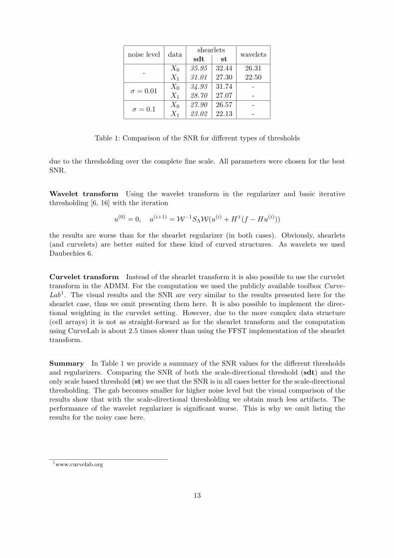
noise level datashearlets

waveletssdt st

-X0 35.95 32.44 26.31X1 31.01 27.30 22.50

σ = 0.01X0 34.93 31.74 -X1 28.70 27.07 -

σ = 0.1X0 27.90 26.57 -X1 23.02 22.13 -

Table 1: Comparison of the SNR for different types of thresholds

due to the thresholding over the complete fine scale. All parameters were chosen for the bestSNR.

Wavelet transform Using the wavelet transform in the regularizer and basic iterativethresholding [6, 16] with the iteration

u(0) = 0, u(i+1) =W−1SΛW(u(i) +HT(f −Hu(i)))

the results are worse than for the shearlet regularizer (in both cases). Obviously, shearlets(and curvelets) are better suited for these kind of curved structures. As wavelets we usedDaubechies 6.

Curvelet transform Instead of the shearlet transform it is also possible to use the curvelettransform in the ADMM. For the computation we used the publicly available toolbox Curve-Lab1. The visual results and the SNR are very similar to the results presented here for theshearlet case, thus we omit presenting them here. It is also possible to implement the direc-tional weighting in the curvelet setting. However, due to the more complex data structure(cell arrays) it is not as straight-forward as for the shearlet transform and the computationusing CurveLab is about 2.5 times slower than using the FFST implementation of the shearlettransform.

Summary In Table 1 we provide a summary of the SNR values for the different thresholdsand regularizers. Comparing the SNR of both the scale-directional threshold (sdt) and theonly scale based threshold (st) we see that the SNR is in all cases better for the scale-directionalthresholding. The gab becomes smaller for higher noise level but the visual comparison of theresults show that with the scale-directional thresholding we obtain much less artifacts. Theperformance of the wavelet regularizer is significant worse. This is why we omit listing theresults for the noisy case here.

1www.curvelab.org

13

(a) noisy and corrupted data X0, σ = 0.1 (b) noisy and corrupted data X1, σ = 0.1

(c) Recovered data X0 with noise level σ =0.1 and only scale based thresholding forΛ = 1

40(0, 0.1, 0.2, 0.4, 1), SNR: 26.57

(d) Recovered data X1 with noise level σ =0.1 and only scale based thresholding forΛ = 1

60(0, 0.1, 0.2, 0.4, 1), SNR: 22.13

(e) Recovered data X0 with noise level σ =0.1 and scale-directional thresholding forα = 1

8, SNR: 27.90

(f) Recovered data X1 with noise level σ =0.1 and scale-directional thresholding forα = 1

6, SNR: 23.02

Figure 8: Numerical results for datasets X0 and X1 with noise σ = 0.114

5 Conclusions

In this paper we apply shearlet regularized image inpainting to recover corrupted seismic data.The provided results show the excellent performance of shearlet regularized inpainting byadditionally using the directional information contained in the shearlet coefficients. Obviouslythis depends heavily on the structure of the missing elements. But seismic data often has strongdirectionality either through different oriented waves or because the different dimensions of thedata represent different measured informations.

References

[1] S. Boyd, N. Parikh, E. Chu, B. Peleato, and J. Eckstein. Distributed optimization andstatistical learning via the alternating direction method of multipliers. Foundations andTrends in Machine Learning, 3(1):1–122, 2011.

[2] E. Candes, L. Demanet, D. Donoho, and L. Ying. Fast discrete curvelet transforms.Multiscale modeling and simulation, 5(3):861–899, 2006.

[3] R. Chan, S. Setzer, and G. Steidl. Inpainting by flexible haar-wavelet shrinkage. SIAMJournal on Imaging Sciences, 1(3):273–293, 2008.

[4] S. Crawley, R. Clapp, and J. Claerbout. Interpolation with smoothly nonstationaryprediction-error filters. In 1999 SEG Annual Meeting, 1999.

[5] S. Dahlke, G. Kutyniok, P. Maass, C. Sagiv, H.-G. Stark, and G. Teschke. The uncertaintyprinciple associated with the continuous shearlet transform. International Journal onWavelets Multiresolution and Information Processing, 6:157–181, 2008.

[6] I. Daubechies, M. Defrise, and C. De Mol. An iterative thresholding algorithm for linearinverse problems with a sparsity constraint. ArXiv Mathematics e-prints, July 2003.

[7] J. Eckstein and D. P. Bertsekas. On the Douglas-Rachford splitting method and theproximal point algorithm for maximal monotone operators. Mathematical Programming,55:293–318, 1992.

[8] D. Gabay. Applications of the method of multipliers to variational inequalities. InM. Fortin and R. Glowinski, editors, Augmented Lagrangian Methods: Applications tothe Solution of Boundary Value Problems, chapter IX, pages 299–340. North-Holland,Amsterdam, 1983.

[9] S. Hauser. Fast finite shearlet transform: a tutorial. Preprint University of Kaiserslautern,2011.

[10] S. Hauser and G. Steidl. Convex multiclass segmentation with shearlet regularization.International Journal of Computer Mathematics, accepted, 2012.

[11] G. Hennenfent and F. Herrmann. Simply denoise: wavefield reconstruction via jitteredundersampling. Geophysics, 73(3):V19–V28, 2008.

15

[12] F. Herrmann and G. Hennenfent. Non-parametric seismic data recovery with curveletframes. Geophysical Journal International, 173(1):233–248, 2008.

[13] M. Kabir and D. Verschuur. Restoration of missing offsets by parabolic radon transform.Geophysical Prospecting, 43(3):347–368, 1995.

[14] G. Kutyniok, K. Guo, and D. Labate. Sparse multidimensional representations usinganisotropic dilation and shear operators. Wavelets und Splines (Athens, GA, 2005), G.Chen und MJ Lai, eds., Nashboro Press, Nashville, TN, pages 189–201, 2006.

[15] Y. Liu and S. Fomel. Seismic data interpolation beyond aliasing using regularized non-stationary autoregression. Geophysics, 76:V69, 2011.

[16] J. Ma and G. Plonka. The curvelet transform. IEEE Signal Processing Magazine,27(2):118–133, 2010.

[17] M. Naghizadeh and K. Innanen. Seismic data interpolation using a fast generalized fouriertransform. Geophysics, 76(1):V1–V10, 2011.

[18] M. Naghizadeh and M. Sacchi. Beyond alias hierarchical scale curvelet interpolation ofregularly and irregularly sampled seismic data. Geophysics, 75(6):WB189–WB202, 2010.

[19] V. Oropeza and M. Sacchi. Simultaneous seismic data denoising and reconstruction viamultichannel singular spectrum analysis. Geophysics, 76(3):V25–V32, 2011.

[20] M. Porsani. Seismic trace interpolation using half-step prediction filters. Geophysics,64:1461, 1999.

[21] J. Ronen. Wave equation trace interpolation. Geophysics, 52(7):973–984, 1987.

[22] M. Sacchi, T. Ulrych, and C. Walker. Interpolation and extrapolation using a high-resolution discrete fourier transform. Signal Processing, IEEE Transactions on, 46(1):31–38, 1998.

[23] S. Setzer. Operator splittings, bregman methods and frame shrinkage in image processing.International Journal of Computer Vision, 92(3):265–280, 2011.

[24] M. Shahram, G. Kutyniok, and X. Zhuang. Shearlab: A rational design of a digitalparabolic scaling algorithm. submitted.

[25] S. Spitz. Seismic trace interpolation in the fx domain. Geophysics, 56(6):785–794, 1991.

[26] R. Stolt. Seismic data mapping and reconstruction. Geophysics, 67(3):890–908, 2002.

[27] G. Tang, R. Shahidi, J. Ma, and F. Herrmann. Applications of randomized sam-pling schemes to curvelet-based sparsity-promoting seismic data recovery,. GeophysicalProspecting, to appear.

[28] D. Trad, T. Ulrych, and M. Sacchi. Accurate interpolation with high-resolution time-variant radon transforms. Geophysics, 67(2):644–656, 2002.

[29] S. Xu, Y. Zhang, D. Pham, and G. Lambare. Antileakage fourier transform for seismicdata regularization. Geophysics, 70(4):V87–V95, 2005.

[30] Y. Yang and et al. et al. Joint l1- and nuclear-norm regularization for seismic datareconstruction. UCLA CAM Report, 2012.

16

[31] Y. Yang, J. Ma, and S. Osher. Seismic data reconstruction via matrix completion. UCLACAM Report 12-14, 2012.

17