Seismic Evaluation of Hydrocarbon Saturation in Deep … - Reservoir... · The focus was on Direct Hydrocarbon Indicators in primarily three categories: 4. What is the proper seismic

September 30, 2004 Seismic Evaluation of Hydrocarbon Saturation in Deep-Water Reservoirs

Grant/Cooperative Agreement DE-FC26-02NT15342.

ANNUAL REPORT

Report Period Start Date: September 1, 2003 Report period End Date: August 31, 2004

Prime Contractor: Colorado school of Mines

Department of Geophysics 1500 Illinois St. Golden, Colorado 80401

Subcontractors: University of Houston

Texas A&M University Industrial Collaborators: Paradigm, Veritas Principal Investigators: M. Batzle - Colorado School of Mines D-h Han - University of Houston (formerly: Houston Advanced Research Center) R. Gibson - Texas A&M University Huw James - Paradigm Geophysical

Agreement DE-FC26-02NT15342, Seismic Evaluation of Hydrocarbon Saturation 1

Disclaimer: This report was prepared as an account of work sponsored by an agency of the United States Government. Neither the United States Government nor any agency thereof, nor any of their employees, makes any warranty, express or implied, or assumes any legal liability or responsibility for the accuracy, completeness, or usefulness of any information, apparatus, product, or process disclosed, or represents that its use would not infringe privately owned rights. Reference herein to any specific commercial product, process, or service by trade name, trademark, manufacturer, or otherwise does not necessarily constitute or imply its endorsement, recommendation, or favoring by the United States Government or any agency thereof. The views and opinions of authors expressed herein do not necessarily state or reflect those of the United States Government or any agency thereof.

Agreement DE-FC26-02NT15342, Seismic Evaluation of Hydrocarbon Saturation 2

Abstract: The "Seismic Evaluation of Hydrocarbon Saturation in Deep-Water Reservoirs" (Grant/Cooperative Agreement DE-FC26-02NT15342) began September 1, 2002. During the second year September 2003-October 2004, we have accomplished several tasks:

- Our second DHI mini-symposium was held at the University of Houston - The Neptune field was added to our set of test sites at the recommendation of Veritas. - Analysis of the Ursa area has begun in depth - Well logs have been acquired from Mineral Management services for blocks 200 near

Troika field in the Green Canyon and blocks 765, 809 and 854 in the Mississippi Canyon - Analog deep-water depositional environments were examined and models developed - The influence of thin bedding on AVO response was modeled - General sand properties were developed and corresponding AVO response established We held our second industry DHI mini-symposium at the University of Houston

sponsored in part by this DOE project. More than 80 representatives attended this symposium from a wide variety of energy and service companies as well as several educational institutions. During this gathering we accomplished several purposes: - Display and disseminate our recent research results - Serve as an informal meeting to exchange ideas and examine current ‘State of the Art’ - Provide a forum to gain feedback and suggestions for our research

So far, we have received several compliments on the success of the meeting. A more complete summary of the symposium is included in the appendix.

Agreement DE-FC26-02NT15342, Seismic Evaluation of Hydrocarbon Saturation

3

Table of Contents: SECTION PAGE Title 1 Disclaimer 2 Abstract 3 Table of Contents 4 List of Figures and Tables 6 Executive Summary 8 Results and Discussion 10

Second DHI Mini-symposium 10

Test Sites 11

Observation of Turbidites in Brushy Canyon Outcrop, West TX 13 Observation of Turbidites in Lewis Shale, Rawlins, Wyoming 15 Comparison of Turbidites in Brushy Canyon to the Lewis Shale Formation 16 Using schematic models as analogs to model a deep-marine basin in GOM 16 Deep-water sand properties and AVO analysis 21 Deep-water sand properties 22 Empirical Model for P-wave velocity 24 AVO modeling: A-B plot 26 Composite Reflection Coefficients 28 AVO analysis after NMO stretch correction 31


4

Plans 40 Conclusions 41 References 41 Appendix DHI mini-symposium abstracts 43


5

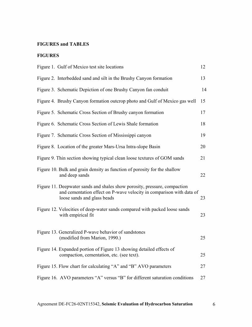
FIGURES and TABLES FIGURES Figure 1. Gulf of Mexico test site locations 12 Figure 2. Interbedded sand and silt in the Brushy Canyon formation 13 Figure 3. Schematic Depiction of one Brushy Canyon fan conduit 14 Figure 4. Brushy Canyon formation outcrop photo and Gulf of Mexico gas well 15 Figure 5. Schematic Cross Section of Brushy canyon formation 17 Figure 6. Schematic Cross Section of Lewis Shale formation 18 Figure 7. Schematic Cross Section of Mississippi canyon 19 Figure 8. Location of the greater Mars-Ursa Intra-slope Basin 20 Figure 9. Thin section showing typical clean loose textures of GOM sands 21 Figure 10. Bulk and grain density as function of porosity for the shallow

and deep sands 22 Figure 11. Deepwater sands and shales show porosity, pressure, compaction

and cementation effect on P-wave velocity in comparison with data of loose sands and glass beads 23

Figure 12. Velocities of deep-water sands compared with packed loose sands

with empirical fit 23 Figure 13. Generalized P-wave behavior of sandstones

(modified from Marion, 1990.) 25 Figure 14. Expanded portion of Figure 13 showing detailed effects of

compaction, cementation, etc. (see text). 25 Figure 15. Flow chart for calculating “A” and “B” AVO parameters 27 Figure 16. AVO parameters “A” versus “B” for different saturation conditions 27


6

Figure 17. Stochastic models considered in the calculation of composite reflection coefficients 29

Figure 18. Composite reflection coefficients for reservoir models that

contain some gas 30 Figure 19. Synthetic seismograms computed for a source/receiver offset

of 25 m 30 Figure 20. Synthetic seismograms computed for a source/receiver offset of

1000 m 31 Figure 21. Synthetic seismograms from a two half-space model with a single

Reflector 34 Figure 22. Comparisons among before NMO, after NMO, and after stretch

Correction 34 Figure 23. Before and after stretch correction 35 Figure 24. Comparison of amplitude distortion in NMO-corrected data 35 Figure 25. Vertical components of full waveform synthetic from Dunkin

(1975)’s model 36 Figure 26. Time-frequency representation of mid (1800 m) and far offset

(2900m) traces 37 Figure 27. Teal South CMP gathers (10981144) before and after stretch

correction. 38 Figure 28. Comparisons of TF analysis for three different frequencies

(20 Hz, 35 Hz, 50 Hz) 39 TABLES Table 1. Current status of Deep-water Fields with seismic hydrocarbon

indicators to be used in this study 11


7

Executive Summary: Our several lines of research are beginning to converge for our Seismic Hydrocarbon Evaluation of Deep-Water Reservoir studies. After considerable effort, seismic data, logs, and core data sets have been obtained for several offshore areas. We are examining several aspects of hydrocarbon assessment including complex layering, fluid properties, attenuation and frequency content. For example, one interesting area has a stack of both productive and uneconomic zones. Seismic data correctly identifies productive reservoirs, but fails to differentiate the uneconomic zones. Fluid properties calculated for realistic conditions show that simple small gas saturations or “Fizz Gas” cannot be responsible for these false indications. This is a joint project involving research at The University of Houston, Texas A&M University, the Colorado School of Mines, and Paradigm Geophysical Corporation. Our strategy is to combine fundamental rock physics concepts and measurements with log, seismic and geologic data from several specific deep-water sites to develop and test more quantitative seismic hydrocarbon saturation indicators. During this second annual project period:

- A second mini-symposium on current and future DHI’s was held at the Univ. of Houston in June 2004

- Log data was acquired for three more sites and generalized geologic sections developed - TGS data for the Ursa field were mounted at UH - A training session was held at Paradigm to familiarize project staff with Paradigm software -Vp models to represent the complex fine scaled bedding in reservoir structures have been

produced - Stochastic models were created to model lateral variations in composite reflection

coefficient for dry and gas saturated layers - NMO stretch correction was applied to synthetic seismic and CMP gathers from Teal South - Synthetic seismograms were generated for each stochastic model (50) with gas bearing

layers for varying offset and frequency - Schematic geologic models of turbidite systems were developed based on outcrop

observations - Preliminary interpretation of Ursa field using seismic lines and well logs - Generalized map of salt structures in Mississippi canyon acquired - General high-porosity sand property trends were established - A flow chart developed for “A” and “B” generation and analysis was produced - The influence of sand and fluid properties on AVO parameters modeled

Our second industry DHI mini-symposium was held at the University of Houston on June 15, sponsored in part by this DOE project. More than 80 representatives attended this symposium from a wide variety of energy and service companies as well as several educational institutions. The focus was on Direct Hydrocarbon Indicators for three categories:


8

1. Examine the proper seismic data acquisition and processing for DHI analysis for true amplitude, true frequency spectrum and phase, elimination or estimation of multiple interference, and practical approaches such as target orientated processing

2. Rock and fluid properties need better calibration. We must accurately

differentiate fluid effects from effects of rock texture (i.e. porosity, cementation, etc.), lithology (shaliness), and reservoir conditions (stress and temperature) on seismic attributes. The best methods to characterize intrinsic attenuation from scattering attenuation are not yet established. We must also improve the seismic evaluation gas saturation.

3. A wide variety of data must be integrated. This includes scaling (frequency)

effects of acoustic velocities, improved seismic ties to log-based synthetics, and better constrained uncertainty of DHIs (Data scattering and statistic evaluation)

More detailed information on the progress and results of this project are also available in the quarterly reports.


9

Results and Discussion: Second DHI Mini-symposium We hosted another Mini-Research Forum at the University of Houston on Direct Hydrocarbon Indicators. This symposium was held on June15 and its purpose was to facilitate new technologies and ideas among interest groups from oil companies, service companies, and universities (including students). These informal presentations (new ideas or data examples) can stimulate and direct efforts in DHI research. The presentations were diverse, and informative. The individual abstracts are presented in the appendix. The focus was on Direct Hydrocarbon Indicators in primarily three categories:

4. What is the proper seismic data acquisition and processing for DHI analysis for a. True amplitude? b. True frequency spectrum and phase? c. Elimination or estimation of multiple interference? d. Practical approaches: target orientated processing

5. Rock and fluid properties a. How accurately can we differentiate fluid effects from effects of rock

texture (i.e. porosity, cementation, etc.), lithology (shaliness), and reservoir conditions (stress and temperature) on seismic attributes?

b. Can we characterize intrinsic attenuation from scattering attenuation? c. Can we evaluate gas saturation seismically? d. How can we ascertain anisotropy?

6. Integration

a. Scaling (frequency) effects of acoustic velocities b. Improved seismic ties to log-based synthetics c. Which seismic attributes are the strongest DHIs d. Can we constrain uncertainty of DHIs (Data scattering and statistic

evaluation) e. How OBC data can help identify hydrocarbon reservoirs?

Other relevant and emerging ideas were also presented (see appendix).


10

Test Sites: As will be seen in this report, we have begun detailed analysis on data from several of our target sites (See Figure 1). Data and samples had to be acquired from several sources and the process is almost complete (see Table 1 below). Seismic data has been obtained from Mobil, Kerr-McGee, TGS, and the ERCH consortium. An additional line is being prepared by Veritas. Recently, samples were obtained from Kerr-McGee and Marathon Oil Companies. Table 1. Current status of Deep-water Fields with seismic hydrocarbon indicators to be used in this study. Field Attribute Status Neptune Producing area with false DHI’s Veritas preparing data for transfer Nansen Core samples & logs available Seismic obtained, Samples meas. Viking Mobil North Sea data with logs Seismic data and logs acquired Ursa Multiple real and false HCI Seismic analysis begun Troika Some data already published Samples Prepared Mars Published data, salt confined Logs obtained Boomvang Near Nansen (Kerr-McGee) Samples & logs obtained Teal South Shelf, only one well, data available Post-stack data and logs at TAMU The Neptune (Viosca Knoll block 826) area is a new addition to the list. This area was suggested by the Veritas staff based on the quality of the seismic data, existence of proven hydrocarbons, as well as false hydrocarbon indicators in the section. The Ursa-Mars-Crosby areas, as we will see below, are all contained within a salt confined minibasin. This proximity will allow a more detailed local geologic model to be developed. The Teal South data had some arbitrary gains and other inappropriate processing performed which render the data of limited value. These data can be used for examples, but complete reprocessing is not practical. The research staff at Veritas is still negotiating with their marine group to obtain the Troika, Mars and Mensa data. The specific lines requested were shown in a previous quarterly report. Additional well logs from lease block 854, 809 and 765 in Mississippi Canyon GOM and Block 200 from Green Canyon GOM were obtained from Mineral Management Services.


11

Figure 1. Gulf of Mexico deep-water test sites. (Modified from Baud et al., 2002)


12

Observation of Turbidites in Brushy Canyon Outcrop Formation, West Texas:

In the last report observations of the Brushy canyon world-class deep-water

outcrops were summarized. Outcrop observations helped contribute to a better understanding of the architectural elements that comprise deep marine basins. The common deep-water characteristics such as inter-bedded sands and silts and sand body (channel) pinch outs are important features to take into account for modeling. Silt beds in the formation varied in thickness from 10 cm to 12m. The thinner silt beds are well beyond seismic resolution. Generally, in stratigraphic interpretation of well logs it is assumed that beds have a more or less uniform thickness across a region. In the Brushy Canyon formation it is clear that this kind of simple analysis will not result in an accurate picture of the subsurface. Bed thickness is highly variable and dependent upon migration of the channel lobe systems through time. (Gardner, et al., 2003) This variability is being taken into account to develop realistic seismic models and help to generate more robust models that represent 3-D changes in the channel lobe systems. Also, detailed geologic information will be used to further develop general models by demonstrating the seismic response to fine scale bedding. An example of the fine scale bedding that was seen in the Brushy Canyon Formation can be seen in Figure 1. This information has provided a good basis for the synthetic seismic models.

Agreement DE-FC26-02NT15342, Seismic Evaluation

Figure 2. Interbedded sand and siltin the Brushy Canyon formation West Texas. Lizard used for scale (length~10 in).

of Hydrocarbon Saturation 13

As was mentioned in the previous report, one of the main shaping features of the deep-water environments is sediment gravity-flows that allow sediments to be carried and deposited by turbidity currents and/or debris flows. Build-Cut-Fill-Spill (BCFS) processes are depositional phases that dominate the evolution and changes in the submarine channel system over time. In the Build phase there is unconfined sediment flow with sediment bypass. Erosion along with sediment bypass with confined flow occurs during the Cut phase. During the Fill phase there is channel deposition. In the Spill phase there is flow deposition that fills the topography (Gardener & Borer, 2000). Figure 2 shows a schematic depiction of changing architectural styles and depositional patterns inferred along the slope and basin

Figure 3. Schematic Depiction of changing architectural styles and depositional patterns inferred along the slope and basin profile of one Brushy Canyon fan conduit. (Gardner et al., 2004). profile of one Brushy Canyon fan conduit. The BCFS model helps to characterize channel body distributions and this characterization can be used to more accurately predict characteristics such as the connectivity and continuity of channel bodies. In a photograph of a Brushy canyon Outcrop (Figure 3.) that shows a sand package on top of a siltstone, it can be seen that the thickness of the sand package varies. The channel is outlined in red and a silt break can be seen inside the sand package. On the right side of the figure, at the channel axis, the sand body is thicker. On the left side of the photo, at the channel margin, the sands get thinner. Sand body distribution becomes important for AVO (Amplitude versus Offset) seismic interpretation because the connectivity of beds will determine location of oil and gas within the reservoir. The Gulf of Mexico gas well to the right of the outcrop photo shows gamma, induction, density and sonic logs. These


14

logs show a good match to the distribution of sands show a good match to the gamma log and show possible fluid distribution for GOM wells based on the sonic log.

Figure 4. Correlation of a photo taken at a Brushy Canyon formation outcrop in West Texas to a Gulf of Mexico gas well showing gamma, induction, density and sonic logs.

Not only do the BCFS depositional phases influence the formation and development of architectural features such as spatial distribution of sand bodies, they also influence rock properties such as lithology, density, sorting, porosity, cementation, and grain size distribution. These properties are important because they can directly affect the seismic response (Batzle and Gardner, 2000). These rock characteristics also control the presence of fluids in the reservoir. In the channel observed in the Brushy Canyon outcrop the grains found near the channel axis were coarser grained than grains located at channel margins (Figure 3). The Brushy Canyon Outcrop photo in Figure 3 shows a good correlation with a Gulf of Mexico gas well. Higher gamma ray readings for the silts compared to the sands due to higher organic content of the silts can be seen. In addition there is a silt break in the sand package that is represented by a peak in the gamma ray. This is just one more example of the variability of thickness in the stratigraphic units that is characteristic of deep-water sediments.


15

Observation of Turbidites in Lewis Shale Formation, Near Rawlins, Wyoming: The Lewis Shale Formation was observed along the eastern margin of the Great Divide basin in south-central Wyoming between Rawlins and Three forks along the US high way 287. The Lewis Shale is one of the major gas reservoirs in the Greater Green River Basin (Anderson, 2004). Although the exposure of these outcrops could not compare to the Brushy canyon outcrops they still offer insight into Delta-Front to slope sediment delivery into the basin that helps to develop a better understanding of the distribution of turbidite sands in the basin. The Lewis formation consists of thin sandstone beds separated by thick shale intervals or dark grey-shales with thin discontinuous carbonate beds, which represent pro-delta/slope deposits. The dad member refers to inter-bedded sandstone/shale units within the middle of the Lewis shale. The dad Sandstone member contains various sandy zones inside of the major Lewis Shale. In this member there is everything from sandstone rich turbidite sheets, that form the major gas reservoirs in the area, to sand and mud rich slope channels, mudstone sheets with thin turbidites, storm and flood derived sandstones, tidal channels and slump derived mouth bars (Anderson, 2004). Comparison of Turbidites in Brushy Canyon Outcrops to Outcrops of the Lewis Shale Formation: The Brushy canyon outcrops prove to be very similar to those in the Lewis Shale formation in the sense that they are both comprised of the inter-bedded sands and shales. The main difference between the two systems is that the Brushy canyon formation is a sand rich system whereas the Lewis shale is a mud rich system. Field observations of these two turbidite systems were used to create schematic geologic models, which have provided a starting point to begin modeling the geologic complexities in turbidite systems. Figures 4 and 5 show schematic geologic models of the Brushy canyon formation and the Lewis Shale formation respectively. The Brushy canyon schematic model was derived from field observations, talks with members of the Brushy Canyon Slope and Basin consortium, and from published data on turbidite systems from Gardner et al. (2003). The Lewis Shale schematic model was derived from field observations, a previously derived stratigraphic section from Reynolds (1976) Lost Soldier area and spoken word with Donna Anderson (2004). Using schematic models as analogs to model a deep-marine basin in the Gulf of Mexico: Preliminary interpretations of the 2-D seismic sections from Ursa field have been preformed and compared with the attributes of deep water systems observed in outcrop. A first pass schematic (Figure 6) of the Ursa section was developed based on the seismic interpretation, well log interpretation of an intersecting well and deep-water outcrop observations. This schematic will be useful to begin synthetic seismic modeling for the GOM Mississippi Canyon. The Ursa well log was hung based on a case history done on the area by Fred Hilterman (2001). Additional well logs from the area have been ordered from Mineral Management services. One well log was obtained from block 200 near


16

Troika field in the Green Canyon. Also wells were ordered from blocks 765, 809 and 854 which are located in the Mississippi canyon. All of these wells lie within ~5 miles of the Ursa well and therefore will aid in developing a depositional profile that maps fine scaled bedding features when interpreted together with seismic profiles found near the TGS seismic lines. The locations of these blocks can be seen in the map in Figure 7 below. One of the major structural complications that occur in the area are salt domes, which are represented by the color green on the map. The salt domes add an additional complexity to the geology because it causes the beds lying on the flanks of the salt domes to dip upwards creating good targets for hydrocarbon plays. Some of these potential hydrocarbon traps have been identified by Hilterman (2001). The schematic models that were derived for the Ursa Field turbidite sequence were sent to TAMU to aid in seismic modeling.

Figure 5. Schematic Cross Section of Brushy canyon formation (Borer, 2004) (Dechesne, 2004) (Slope and Basin consortium Website, 2004)


17


18

Figure 6. Schematic Cross Section of Lewis Shale formation (Anderson, 2004) (Reynolds, 1976)


19

Figure 6. Schematic Cross Section of Gulf of Mexico Mississippi Canyon Ursa Field Figure 7. Schematic Cross Section of Mississippi canyon basin (Anderson, 2004) (Meckel et al., 2002)


20

Figure 8. Location of the greater Mars-Ursa Intraslope Basin. The dark line on the regional map highlights the Mississippi canyon area. Red Squares show unit boundaries of producing fields. Green areas represent salt structures. White areas are unaffected by salt structures. (Meckel et al., 2002)


21

Deep-water sand properties and AVO analysis We have systematically investigated properties of deep-water reservoir sand properties. We have gained a significant understanding of how the turbidite depositional environment affects sand properties. Based on those properties, we have developed a rock physics model for AVO analysis. Influence of geological environment on deep-water reservoirs The geological environment of deep-water turbidite sand reservoirs has distinct characteristics:

1. Depth: deep-water reservoirs are typically beyond continental shelves with water depths anywhere from 300 m to more than 3000 m.

2. Sediments are typically young (Pliocene…). 3. Reservoirs are often associated with high pore pressure (relatively low differential

pressure relative to the depth). 4. Typically, this is a low temperature environment. 5. Early hydrocarbon saturation often prevents the normal cementation process.

Turbidite sands often show features such as fine grain sands with grains sizes of approximately 100 microns, moderate sorting, relatively clean without clays, and with no or weak cementation. (Figure 9:thin section image) The loose sands have a wide range of porosity from 35% to 25% (Figure 10) depended mainly on depth and age (progressive compaction with differential pressure), grain sorting (potential for elastic compaction). The VHP sands are from depth of 12000 ft and The HP sands are from depth of 18,000 ft. Both sands are weakly cemented with a range of porosity controlled by sorting. Permeability of the sands ranged from a high of near 1000 md to a low of 100 md.

Figure 9. Thin section showing typical clean loose textures of GOM sands


22

ShallowDeep

Sorting

HP

Shale

VHP

Figure 10: Bulk (Db)and grain (Dg) density as function of porosity for the shallow and deep sands

Deep-water sand properties Measured data for dry velocities of the deep-water sands are shown in Figure11.

1. Porosity is progressively reduced with depth from 35% at shallow depths to around 24% at greater depths. As a comparison, repacked loose sands (LS) in the laboratory show a high porosity of 40% in initial packing and compacted to 37 to 36% at high pressure.

2. P-wave velocity shows progressive increase with decreasing of porosity. High velocities of the high porosity sands are due to high pressure of 4000 psi in comparison to 2000 psi for low velocities of the very high porosity sands. Data show strong differential pressure effect on velocity. However, velocities increase slightly with decreasing porosity. It suggests that without increasing cementation, compaction does not contribute much to increased rigidity and stiffness of rock frame and velocities.


23

LS

HP

Shale

VHP

Figure 11. Deepwater sands and shales show porosity, pressure, compaction and cementation effect on P-wave velocity in comparison with data of loose sands and glass beads.

5.005.0 )/)*1

(()/( ρϕ

ρn

MMV+

==

Figure 12. Velocities of deep-water sands compared with packed loose sands with empirical fit.


24

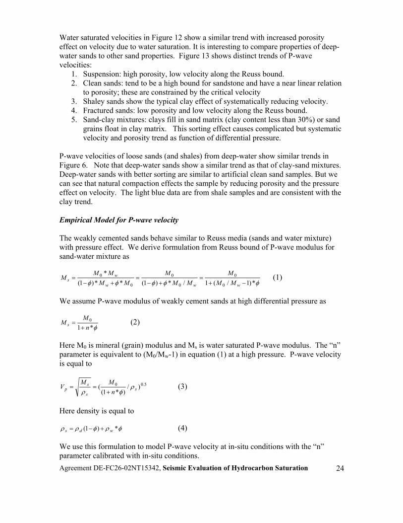
Water saturated velocities in Figure 12 show a similar trend with increased porosity effect on velocity due to water saturation. It is interesting to compare properties of deep-water sands to other sand properties. Figure 13 shows distinct trends of P-wave velocities:

1. Suspension: high porosity, low velocity along the Reuss bound. 2. Clean sands: tend to be a high bound for sandstone and have a near linear relation

to porosity; these are constrained by the critical velocity 3. Shaley sands show the typical clay effect of systematically reducing velocity. 4. Fractured sands: low porosity and low velocity along the Reuss bound. 5. Sand-clay mixtures: clays fill in sand matrix (clay content less than 30%) or sand

grains float in clay matrix. This sorting effect causes complicated but systematic velocity and porosity trend as function of differential pressure.

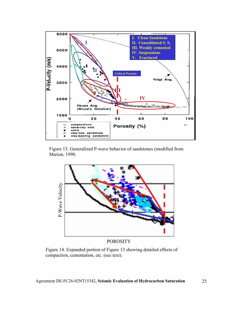
P-wave velocities of loose sands (and shales) from deep-water show similar trends in Figure 6. Note that deep-water sands show a similar trend as that of clay-sand mixtures. Deep-water sands with better sorting are similar to artificial clean sand samples. But we can see that natural compaction effects the sample by reducing porosity and the pressure effect on velocity. The light blue data are from shale samples and are consistent with the clay trend. Empirical Model for P-wave velocity The weakly cemented sands behave similar to Reuss media (sands and water mixture) with pressure effect. We derive formulation from Reuss bound of P-wave modulus for sand-water mixture as

φφφφφ *)1/(1/*)1(**)1(*

0

0

0

0

0

0

−+=

+−=

+−=

www

ws MM

MMM

MMM

MMM (1)

We assume P-wave modulus of weakly cement sands at high differential pressure as

φ*10

nM

M s += (2)

Here M0 is mineral (grain) modulus and Ms is water saturated P-wave modulus. The “n” parameter is equivalent to (M0/Mw-1) in equation (1) at a high pressure. P-wave velocity is equal to

5.00 )/)*1(

( ss

sp n

MMV ρ

φρ +== (3)

Here density is equal to

φρφρρ *)1( wds +−= (4)

We use this formulation to model P-wave velocity at in-situ conditions with the “n” parameter calibrated with in-situ conditions.

Agreem

I

II

III

I. Clean SandstoneII. Consolidated S. S.III. Weakly cementedIV. SuspensionsV. Fractured

Critical Porosity

V

IV

Fc

Figure 13. Generalized P-wave behavior of sandstones (modified fromMarion, 1990.

ent DE-FC26-02NT15342, Seismic Evaluation of Hydrocarbon Saturation 25

POROSITY

P-W

ave

Vel

ocity

igure 14. Expanded portion of Figure 13 showing detailed effects of ompaction, cementation, etc. (see text).


26

AVO modeling: A-B plot

We model Amplitude Versus Offset characterization with Shuey’s equation.

2)(*)( θθ SinBAR += (5)

Where A is the normal reflection coefficient, B is the gradient of amplitude versus incident angle. Based on shale and sand interface, we can build rock models to correlate

1. Shale properties: based on log data we can derive Vp, Vs, porosity and density of shale cap and we assume those properties remain nearly constant through the interface.

2. Reservoir pressure and temperature conditions.

3. Brine properties: density and bulk modulus based on salinity and in situ conditions.

4. Hydrocarbon properties: we use gas density and bulk modulus at in situ conditions.

5. We select “n” parameter to model in A-B plot for wet sands (water zones).

6. We perform the following steps to predict porosity and different fluid saturation effects.

a. Derive dry P-wave modulus based on wet modulus and brine properties using modified Gassmann’s equation (Han and Batzle, 2004)

b. Calculate dry bulk modulus based the dry P-wave modulus (Han and Batzle, 2004)

c. Do fluid substitution for different fluid combination.

d. Perform the above calculation variation of porosity.

Figure 15 shows the flow chart to generate A-B plot as shown in Figure 16. This model constrains how the above parameters affect A-B distribution, such as:

1. Increase “n” value will cause increasing A (absolute value)

2. Increasing porosity will cause increase A and decrease B (absolute value).

3. Increase gas saturation: large effect with small amount of gas (10-30%). High gas saturation will cause high A value but less effect on B value.

Quantitative measure of the normal reflection coefficient may be the best gas indicators.


27

Ms_w

Md

µ

Kd

Ks

Vp, Vs, ρ

Vp, Vs, ρ

A & B

Shale

Sandstone

Sandstone

Kw,Kf, Sw

φ*10

nM

M s +=

Figure 15. Flow chart for calculating “A” and “B” AVO parameters

Figure 16. AVO parameters “A” versus “B” for different saturation conditions


28

Composite Reflection Coefficients

Our previous reports have presented illustrations of composite reflection coefficients computed for reservoirs that are modeled as stacks of thin layers. The general goal of this approach is to quantify the influence of internal reservoir heterogeneity on amplitude variation with offset (AVO) analyses. Because conventional AVO studies assume that the seismic reflection amplitudes can be modeled using approximate expressions for a plane wave reflecting from a single, planar boundary, there is likely some error when examining field data that is acquired from more complex reservoir structures. As an example, consider the model shown in Fig. 1. It includes a heterogeneous reservoir zone that is 30 m thick, divided into 30 layers 1 m in thickness. The average velocity in the reservoir layer is 2.9 km/s, while the velocity of the two layers above and below is 2.7 km/s. The compressional and shear seismic velocities of each of the 30 internal reservoir layers are chosen randomly from a Gaussian distribution. Furthermore, each layer has a 30% chance of containing natural gas; otherwise the layer is assumed to contain brine. In either case, conventional fluid substitution using the Gassmann equation is applied to specify the velocities. Using the propagator matrix methods described in previous reports, we compute the reflection P-wave composite reflection coefficient for the entire layer stack. This method provides a simple scheme for generating the amplitude of the P-wave signal reflected by the entire stack of layers representing the reservoir. In contrast, typical AVO analysis would model the reflection as originating only from the first boundary. Because many geologic environments will result in fairly complex, variable vertical layering in the reservoir, it is important to quantify the variation in reflection coefficient that may result. To do so, we generated a suite of 50 stochastic models of the type shown in Fig. 17, and the resulting reflection coefficients at a frequency of 30 Hz are shown in Fig. 2 (green curves). This figure also compares the results to composite reflection coefficients for a model that does not contain gas-bearing internal layers (red curves). There are several interesting points in these results. First, the presence of gas will result in larger amplitude P-wave reflections, because the fluid significantly decreases the P-wave velocity. This leads to “bright spots” in field data. However, comparing the two models results in Fig. 18, we can see that it also introduces more scatter into the predicted reflection response as a function of angle of incidence. In other words, there is a greater degree of variation in the green curves than the red, and this shows that location and distribution of the gas-bearing layers in the reservoir, which are randomly chosen in these models, has a strong influence on the interactions of waves reflected from each layer. It is also extremely encouraging to note that even though there is scatter in the reflection coefficient, the mean trend of the curves for each model are still consistently different, providing some support for why AVO methods can work even when the earth is not particularly similar to the idealized model with a single interface. Synthetic seismograms were also generated for each of the 50 models with gas-bearing layers (Figs. 19, 20). These waveforms also reveal several important properties of the model. First, we should note that computing a composite reflection coefficient only makes sense for relatively low frequencies, in which case the seismic wavelength is greater than the thickness of the reservoir. The reflections from the top and bottom of the reservoir, as well as all internal boundaries, then superpose to create a single event in the seismic section; this is commonly referred to as “tuning”. Because the effects of this


29

tuning depend on the ratio of wavelength to layer thickness, the seismograms should also be frequency dependent, and we therefore computed results for several source wavelet frequencies, 15, 30 and 60 Hz. For clarity, a subset of 15 seismograms are shown in each panel. The plots show clearly that there is more scatter in the seismic amplitudes at higher frequencies, which is reasonable, since the wavelength is closer to the size of the reservoir. In this case, the details of the arrangement and properties of internal layers have a stronger influence on the wave field. Comparing results for receivers at near offset (25 m, Fig. 19) and far offsets (1 km, Fig. 20), we see that the primary difference in this case is that the amplitudes are somewhat larger at the more distant receiver. This is consistent with the composite reflection coefficients in Fig. 18, where amplitude also increases slightly with offset. Note that the offset of 1 km corresponds to an angle of incidence of 30 degrees, so that the square of the sine is 0.25.

Figure 17. Representative example of the stochastic models considered in the calculation of composite reflection coefficients. The reservoir includes 30 layers that are 1 m thick, and each has a 30% chance of containing natural gas.


30

Figure 18. Composite reflection coefficients for reservoir models that contain some gas (green) and those containing only brine (red).

Figure 19. Synthetic seismograms computed for a source/receiver offset of 25 m for 15 models of the types shown in Fig. 17. Corresponding predicted composite reflection coefficients are in Fig. 18 (green curves).


31

Figure 20. Synthetic seismograms computed for a source/receiver offset of 1000 m for 15 models of the types shown in Fig. 17. Corresponding predicted composite reflection coefficients are in Fig. 18 (green curves). AVO analysis after NMO stretch correction Attenuation is becoming one of the most important subsurface properties because of its sensitivity to fluid saturation. Attenuation makes seismic amplitude frequency-dependent along with wave propagation effects. In our previous study, we analyzed AVO cross-plots for three band-pass filtered data and pointed out that frequency changes by NMO stretch had to be corrected first for meaningful interpretations. There were two approaches to correct the NMO stretches: a wavelet deconvolution-based method (Castoro et. al., 2001) and a stretch-free NMO (Trickett, 2003). It is very likely that wavelet deconvolution-based method will change the frequency dependence of AVO because the frequency contents of estimated wavelet would be different from those of attenuated wavelets of our interest. Furthermore, our field data (from Teal South) was provided with the NMO correction already applied. As a result, our approach is to devise a scheme that can be used on top of the existing processing flow after the application of conventional NMO corrections. Our algorithm is a two-step process. First, we identify reflections of our interest and second, correct amplitude and frequency information using a shift scheme based on the magnitude of the estimated stretch ratio. After the target oriented NMO stretch correction, we expect class III AVO anomalies in the data will show more accurate frequency dependence, while the class I and II will show the decreased normal incident and gradient attributes.


32

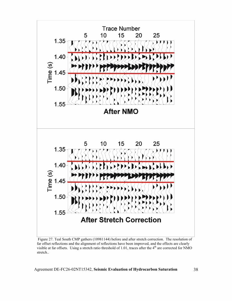
A full waveform synthetic seismogram computed for a two half-space model has been computed to test the idea. Fig 21 shows the NMO corrected synthetic data in this model. To test the effectiveness and possible problems of this algorithm, an extreme case (shallow and far offset trace) is considered. As traces approach far offset, the widths of the wavelets were increased by the NMO stretch. Two 3000 m offset traces (before and after NMO) are shown in Fig 22a. In this ideal case, exact values for stretch ratio and amplitude before NMO are known. The numerical estimation of stretch ratio and the exact stretch ratio that is computed from synthetics are shown at Fig 22b. The stretch ratio can be estimated quite accurately using the equations from Dunkin (1975). As shown in our previous report, by shifting the Fourier components with this stretch ratio amount, we can reverse the NMO stretch effect (Fig 21b). Amplitude values before NMO, after NMO, and after stretch correction are shown in Fig 22. Fig 23 shows two fundamental attributes in the above three cases (before NMO, after NMO, after stretch correction). Magnitude spectra clearly show low frequency signal in the trace after NMO correction. Also, the phase spectra show almost constant shifts over all frequencies after the stretch correction has been applied. To simplify AVO analysis, we also align corrected wavelets using time shifts from cross-correlation measurements at the last stage of this algorithm. This will automatically improve the event alignment for better stack results. The percent error after the stretch correction (Fig 24a) shows less than 5% amplitude errors over all offset ranges compared with ~40% error at 3000 m offset. For better quantification of amplitude and frequency, time-frequency representation based on wavelet matching (Liu et. al., 2004) is used (Fig 24b-d). After the stretch correction, amplitude and frequency information matches very well while the after NMO trace shows severe distortions in amplitude and frequency. A multi-layered model from Dunkin (1975) has been used to study the amount of NMO stretch effects with different offsets and depths (Fig 25). The severe distortions of wavelets in the first shallow event are clearly visible, while the amount of stretch decreases with depth (less distortion). For comparison purposes, only strong signals (1st, 3rd, 4th, and 6th) were stretch-corrected. The time-frequency representations are shown in Fig 26 on mid-offset (1800 m) and far offset (3000 m). As expected, severe distortions in amplitude and frequency on traces from far offset and shallow events were observed and corrected. In our previous study of the Teal South field data, examination of the low frequency data showed a strong amplitude increase with offset while high frequency data exhibited almost no increase in amplitude with offset, perhaps even including a decrease with offset. We concluded that this observation was a consequence of the NMO stretch artifacts. Our target oriented stretch correction has been applied to several CMP gathers (Fig 27). Several factors make application of the correction to the field data more difficult than for synthetic seismograms, including (1) severe mute of input data, (2) low S/N ratio, (3) non-regular offsets. After careful choices of stretch ratio threshold, application window length, and taper size, the result of stretch correction is shown in (Fig 27b). Narrower wavelets are clearly visible at the far offsets and the alignment of events was significantly improved. Time-frequency analysis from the wavelet matching is shown in Fig 28. By comparing relative amplitude with offset at ~1.42 sec, we can see a clear difference at the 50 Hz plot. Before stretch correction, the amplitude changes from strong to weak (Fig 28c). On the other hand, the amplitude changes from strong to strong can be observed


33

after the stretch correction (Fig 28f). Further tests using Paradigm’s Probe software (cross plots of AVO attributes) are under investigation to better understand these changes. In conclusion, for a better amplitude and frequency analysis, NMO stretch corrections based on simple frequency shift (target oriented NMO stretch corrections) are successfully applied to simple synthetics and several reflections of our interest (4500 ft sand) in Teal South data. Stretch ratios can be accurately estimated and our objective is to compare AVO anomaly patterns after addressing this processing artifact. Our current algorithm can be considered as a quick fix, but it is more proper than wavelet deconvolution based methods: the latter might change the frequency contents significantly. The field data application clearly showed changes in amplitudes with offset after the stretch correction, which result in the increase of gradient attribute especially in high frequency region.

Agreeme

Figurcorreafter

Figuroffseestimbefor

e 21. Synthetic seismograms from a two half-space model with a single reflector. (a) NMO cted shot gather, (b) Stretch corrected shot gather. Notice wider wavelets with increasing offset NMO, and the narrowing of the same wavelets after stretch correction.

e 22. Comparisons among before NMO, after NMO, and after stretch correction. (a) 3000 m t traces (before NMO and after NMO), (b) Stretch ratio (blue: computed from input data, red: ation using Dunkin (1975) equation), (c) and (d), Absolute maximum amplitude of wavelets of e NMO (blue), after NMO (red), and after stretch correction (black).

nt DE-FC26-02NT15342, Seismic Evaluation of Hydrocarbon Saturation 34


35

Figure 23. (a) Magnitude spectra, (b) Phase spectra: before NMO (blue), after NMO (red), and after stretch correction (black), (c) Phase ratio between after stretch correction and before NMO, (d) Phase ratio between after stretch correction and after NMO. Almost constant phase delay can be observed after the stretch correction.

Figure 24. Comparison of amplitude distortion in NMO-corrected data before (blue) and after stretch correction (red) (Upper left). Also shown are time-frequency analyses based on wavelet matching, showing results for a trace at an offset of 3000 m, before NMO correction (i.e., input data), after NMO is applied, and, finally, after stretch correction of the NMO signal (lower right). The stretch correction accurately reconstructs the spectral content of the input signal.


36

Figure 25. Vertical components of full waveform synthetic from Dunkin (1975)’s model. After the target oriented stretch correction, resolution has increased. Note that only 1st, 3rd, 4th, and 6th events were stretch-corrected and AGC has applied to see waveforms of deeper events better.


37

Figure 26. Time-frequency representation of mid (1800 m) and far offset (2900m) traces from Dunkin (1975)’s model. For comparison, only 1st, 3rd, 4th, and 6th events were stretch-corrected. As expected, shallow and far-offset events show large amount of corrections. No AGC has applied to the input synthetic in these TF representations.


38

Figure 27. Teal South CMP gathers (10981144) before and after stretch correction. The resolution of far offset reflections and the alignment of reflections have been improved, and the effects are clearly visible at far offsets. Using a stretch ratio threshold of 1.01, traces after the 4th are corrected for NMO stretch..


39

Figure 28. Comparisons of TF analysis for three different frequencies (20 Hz, 35 Hz, 50 Hz). Left column: before stretch correction. Right column: after stretch correction. Notice the relative amplitude increase at 50Hz data after the stretch correction. Phase I of CMP 11041150. Each plot has been normalized to the maximum value between 1.35-1.55 sec.


40

Plans: We are continuing with our initial goals of acquiring sets of samples with appropriate seismic and log data. Members of the research team accepted responsibilities for individual tasks for the next period: R. Gibson (TAMU) - Specify and transfer seismic data from Veritas

- Continue wavelet frequency analysis of seismic data - Continue forward modeling with site-specific parameters - Extend thin bed models to logged sections around reservoirs

D. Han (UH) - Develop rock physics models to calibrate AVO response

- Apply results to the Nansen field data - Develop schemes to assess AVO data quality - Improve inversion procedures to identify ‘fizz’ gas - Make additional ultrasonic measurements on sands

M. Batzle (CSM) - Continue development of deep-water geologic models

- Forward model Assist in transfer of seismic data from Veritas - Obtain remaining logs from test sites - Continue log data analysis including fluid substitution - Measure Troika samples (ultrasonic) - Begin low-frequency measurements

Duane Dopkin - Define ‘true frequency’ processing (Paradigm) - Evaluate seismic data quality

- Organize seismic analysis examples and training - Develop reprocessing procedures

Further information can be obtained from:

Dr. Michael Batzle Colorado School of Mines

Phone: 303-384-2067 email: [email protected]

References


41

Allen, James L. and Peddy, Carolyn P. Amplitude Variation with offset: Gulf coast Case Studies. Geophysical development Series, Volume 4 SEG Anderson, Donna. Colorado School of Mines Lewis Consortium Field Trip Guide: Delta-Front to slope sediment delivery into the basin. July 31-August 1 2004. AAPG memoir 26 Seismic Stratigraphy-Applications to hydrocarbon Exploration 1977 Baud, R.D., and others, 2002, Deepwater Gulf of Mexico: America’s expanding frontier: Mineral Management Service OCS report MMS 2002-021.

Borer, Jim. Personal communication. July 20, 2004.

Dechesne, Marieke. Personal communication. July 20, 2004. Gardner, M.H., and Batzle, M., 2003 Lithology and Fluids: Seismic Models of the Brushy Canyon Formation West Texas Gardner, M.H., Borer, J.M., Melick, J.J., Mavilla, N., Dechesene, M., and Wagerle, R.N., 2003, Stratigraphic Process Response model for submarine channels and related features from studies of Permian Brushy Canyon outcrops, West Texas: Marine and Petroleum Geology, 20, 757-787. Gardner. H., Borer, J.M., 2000, Submarine channel architecture along a slope to basin profile, Brushy Canyon Formation, West Texas, in A.H. bouma and CG Stone, eds., Fine-Grained turbidite systems, AAPG Memoir 72/SEPM Special Publication No. 68, p 195-214. Gardner, M.H., June 29, 2004. Slope and Basin Consortium Website Colorado School of Mines: Resource Optimization of Slope and Basin Reservoirs through Enhanced Imaging of Reservoir Architecture http://www.mines.edu/Academic/geology/sbc/index.shtml Gassmann, F., 1951, Uber die Elastizitat poroser medien. Veri der nature Gesellshaft Zurich, 96, 1-23.

Han, D. and Batzle, M, 2004: Gassmann’s equation and fluid saturation effects, Geophyiscs. V. 69,

Han, D., and Batzle, M., 2004: Estimate shear velocity based on P-wave and Shear modulus relationship. Presented at SEG annual meeting at Denver. Hilterman, F. Seismic Amplitude Interpretation 2001 Distinguished Instructor Short Course Series no. 4 EAGE 2001 Keys Robert G and Foster Douglas J. Comparison of Seismic Inversion methods on a Single real data Set. SEG 1998


42

Liu, J., Wu, Y.,Han, D., Li, X., 2004, Time-frequency decomposition based on Ricker wavelet, 74th Ann. Internat. Mtg.: Soc. of Expl. Geophys. Meckel, L.D., III, Ugueto, G. A., Lynch, H. D.,cumming, E.W. Hewett, B. M., Bocage, E.J., Winker, C.D., O’neill, B.J.. Genetic Stratigraphy Architecture and Reservoir Stacking Patterns for Upper Miocene-Lower Pliocene Greater mars-Ursa Intraslope Basin Mississippi Canyon, Gulf of Mexico . 22nd Annual gulf Coast Section SEPM Foundation Bob F Perkins research Conference-2002. p 113-146. Reynolds, M. W., 1976, Influence of recurrent Laramide structural growth on sedimentation and petroleum accumulation, Lost Soldier area, Wyoming: AAPG Bulletin, v. 60, p. 12-33 Rupert, G. B. and Chun, J. H., 1975, The block move sum normal moveout correction: Geophysics, Soc. Of Expl. Geophys., 40, 17-24 Trickett, S., 2003, Stretch-free stacking, 73rd Ann. Internat. Mtg.: Soc. of Expl. Geophys., 2008-2011.


43

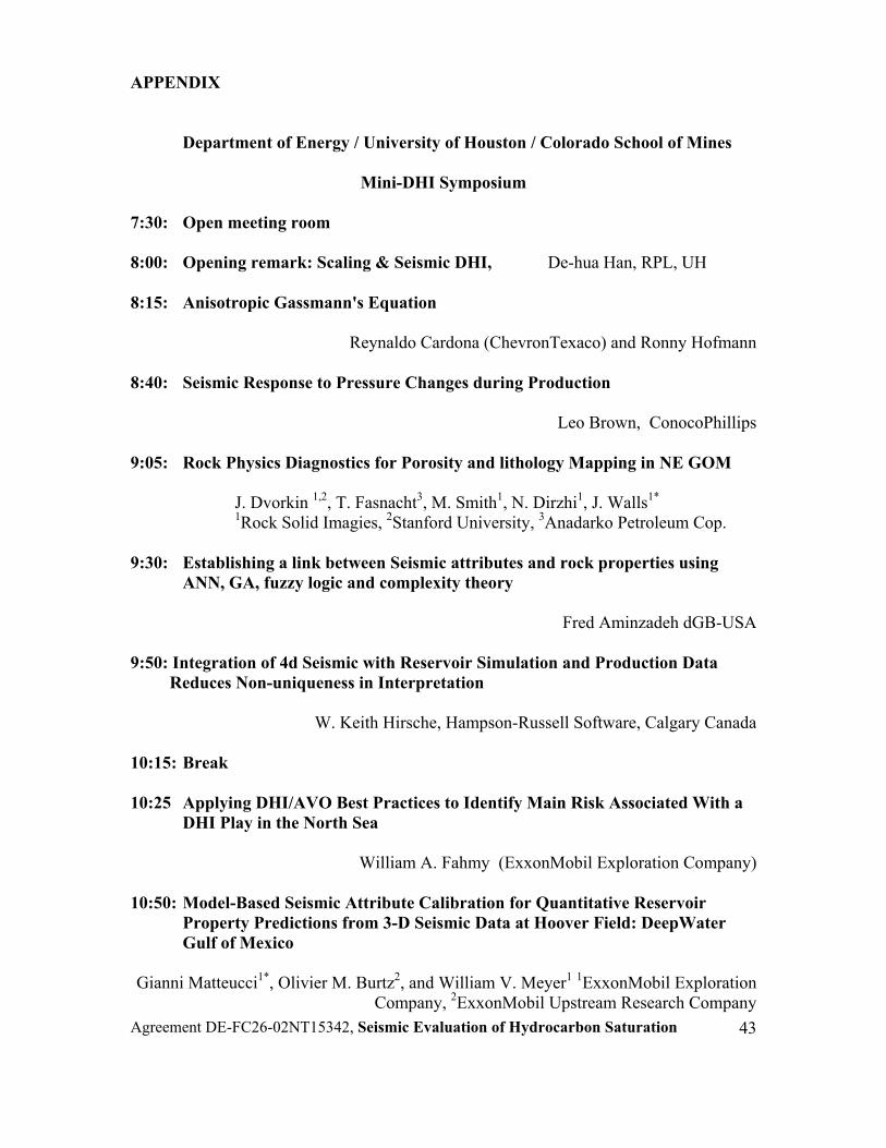
APPENDIX Department of Energy / University of Houston / Colorado School of Mines

Mini-DHI Symposium

7:30: Open meeting room 8:00: Opening remark: Scaling & Seismic DHI, De-hua Han, RPL, UH 8:15: Anisotropic Gassmann's Equation

Reynaldo Cardona (ChevronTexaco) and Ronny Hofmann

8:40: Seismic Response to Pressure Changes during Production

Leo Brown, ConocoPhillips 9:05: Rock Physics Diagnostics for Porosity and lithology Mapping in NE GOM

J. Dvorkin 1,2, T. Fasnacht3, M. Smith1, N. Dirzhi1, J. Walls1* 1Rock Solid Imagies, 2Stanford University, 3Anadarko Petroleum Cop.

9:30: Establishing a link between Seismic attributes and rock properties using

ANN, GA, fuzzy logic and complexity theory

Fred Aminzadeh dGB-USA 9:50: Integration of 4d Seismic with Reservoir Simulation and Production Data

Reduces Non-uniqueness in Interpretation

W. Keith Hirsche, Hampson-Russell Software, Calgary Canada 10:15: Break 10:25 Applying DHI/AVO Best Practices to Identify Main Risk Associated With a

DHI Play in the North Sea

William A. Fahmy (ExxonMobil Exploration Company)

10:50: Model-Based Seismic Attribute Calibration for Quantitative Reservoir Property Predictions from 3-D Seismic Data at Hoover Field: DeepWater Gulf of Mexico

Gianni Matteucci1*, Olivier M. Burtz2, and William V. Meyer1 1ExxonMobil Exploration

Company, 2ExxonMobil Upstream Research Company


44

11:15: Current seismic method and its limitation: carbonate and clastic under

carbonate August Lau, Apache Cop.

11:40: Reconnaissance of geological prospectivity and reservoir characterization

using multiple seismic attributes on 3-D surveys: an example from hydrothermal dolomite, Devonian Slave Point Formation, northeast British Columbia, Canada

Strecker1, U., Knapp2, *, S., Smith1, M., Uden1, R., Carr1, M., Taylor1, G.

1Rock Solid Images, 2Seitel Incorporated 12:05: Discussion 12:15: Lunch Break 1:10: Wave dispersion and Attenuation 1:20: VSP Velocity and Absorption Analysis using a Phase Spectral Method

Yingping Li, VSFusion, A Baker Hughes – CGG Company 1:45: Seismic Attenuation in a Fractured Oil Reservoir of Northeastern Mexico

form a Time-Frequency Analysis

Dr. Rual del Valle Garcia, IMP 2:25: Seismic Scattering Theory Applied to AVO and Seismic-Well Correlations In Thin-Beds

D.J. Foster and F.D. Lane, ConocoPhillips Basin Modeling Methods and Seismic Inversion Methods: Integrating two Technologies to Reduce Prospect Risk

Xin-Gong Li, UH and IntSeis, Inc., Tim Matava, L & W Geosciences 2:50: Discussion 3:00: Break


45

3:10: Composite Reflection Coefficients, Attenuation and Frequency Dependent AVO

Richard Gibson, Dept. of Geology & Geophysics Texas A&M University 3:35: Imaging and AVO analysis of the Marmousi2 Elastic Model

Gary Martin, GXT & AGL, UH 4:00: Extending Geometric Attributes to Illuminate Lithology in Bright Spots.

Kurt J. Marfurt AGL, UH

4:25: Discussion

4:50: Adjourn


46

Opening remarks: Scaling & Seismic DHI De-hua Han, RPL, UH Geological heterogeneity presents on layers and complicated geometry. Hydrocarbon fluids induce complicated fluid distribution. All those heterogeneity cause seismic wave dispersion intrinsically and scattering. As we use seismic attributes to quantitatively estimate reservoir parameters such as saturation, porosity, pressure… we may have to recheck basic assumptions been dominate in the seismic techniques. Anisotropic Gassmann's Equation

Reynaldo Cardona (ChevronTexaco) and Ronny Hofmann Rock Physics Diagnostics for Porosity and lithology Mapping in NE GOM J. Dvorkin 1,2, T. Fasnacht3, M. Smith1, N. Dirzhi1, J. Walls1 1Rock Solid Imagies, 2Stanford University, 3Anadarko Petroleum Cop. Summary We apply a rock physics analysis to well log data from the North-East Gulf of Mexico to establish an effective medium transform between the acoustic and elastic impedance on one hand and lithology, pore fluid and porosity on other hand. Those transforms are upscaled and applied to acoustic and elastic impedance inversion volumes to map lithology and porosity. Establishing a link between Seismic attributes and rock properties using ANN, GA, fuzzy logic and complexity theory Fred Aminzadeh dGB-USA, 1 Sugar Creek Center Blvd., Suite 935, Sugar Land, TX 77478, [email protected] Abstract


47

We will introduce the meta-attribute concept for combining “artificial intelligence” of neural networks with the “natural intelligence” of an interpreter. This leads to a more comprehensive integration of geological, petrophysical, rock physics and seismic data. Non-linear interrelationships between data as well as knowledge versus geologic features and reservoir properties are defined implicitly at the natural scale level. Meta attributes extracted from multiple input seismic volumes and derived attributes are used to predict porosity lithology or fluid saturation, as well as for detecting faults, fractures, channel facies or salt bodies. Some possible future research topics to further facilitate applications of alternative methodologies will be discussed. Specifically, the role that genetic algorithm (genome), fuzzy logic and complexity theory can play in addressing many challenging issues such as scale and uncertainty issues, will be explored. "Seismic Response to Pressure Changes during Production" Leo Brown, ConocoPhillips Time-Lapse seismic experiments ideally lead to interpreted fluid saturation and pore pressure change in the reservoir. Modeling of fluid changes with pore pressure and dry rock moduli changes with effective stress are usually done independently and the results recombined with Gassmann's equation. Pressure change can be modeled with empirical equations, crack models, or grain-contact models such as Hertz-Mindlin. An adaptation of the uncemented sand model, which is based on Hertz-Mindlin for pressure dependence and the Hashin-Shtrikman lower bound for porosity dependence, is presented. The pressure sensitivity exponent, rather than the fixed 1/3 in the Hertz-Mindlin model, can be calibrated based on experimental data. This flexibility allows good matching of the pressure sensitivity of a wider range of rocks than Herz-Mindlin theory. Examples are shown for a variety of sandstones and carbonates. INTEGRATION OF 4D SEISMIC WITH RESERVOIR SIMULATION AND PRODUCTION DATA REDUCES NON-UNIQUENESS IN INTERPRETATION W. Keith Hirsche, Hampson-Russell Software, Calgary Canada Time Lapse seismic interpretation is often complicated because the technique measures changes in the seismic response (caused by changes in acoustic velocity and density) between surveys while the engineer requires information about the pressure, temperature and saturation changes in the reservoir. Rock physics and seismic modelling provide an important bridge between the engineering parameters and the seismic response. However, the relationships are often non-unique because the same changes in acoustic parameters can be caused by a range of pressure, temperature and saturation changes in the reservoir rocks. Reservoir engineering and production data can often provide useful information to


48

help constrain the 4D seismic interpretation by providing physical limits on the saturation and pressure changes that have occurred in the reservoir. The reservoir engineering data can be included through simple material balance or volumetric approaches or by a quantitative comparison of the reservoir simulation predictions and the time-lapse seismic interpretations. When seismic interpretation and reservoir simulation are tightly coupled, non-uniqueness in both the reservoir simulation history matching cycle and also the time-lapse interpretation process is reduced. Current seismic method and its limitation: carbonate and clastic under carbonate August Lau, Apache Corporation University of Houston Symposium 2004 We will discuss current seismic method in a high level sense using 2 examples: one from carbonate and another one from clastic under carbonate. The first example is carbonate where the pay zone is 5-20 meters. Much research in carbonate is devoted to thicker reservoir (>50 meters). Statistically, there are many carbonate fields, which have thinner pays and have great business impact. We will show an example. The second example is clastic reservoir under carbonate. Again, we want to emphasize that the average pay thickness is about 5-20 meters. Statistically, this is where our interest is and its understanding has great business impact. North Sea Jurassic under chalk is a good example and prestack inversion has been used to image sand under chalk. The thick sands under carbonate have been largely found and easier to identify. But what is left is the thinner sand under carbonate. Current seismic method uses seismic modeling (example 1) and prestack inversion (example 2). They have been useful but applicable to simple topology. When we encounter complex topology (e.g. carbonate reflection and transmission), it has scale lengths of all sizes. We need to find better method since the mathematics of modeling and inversion has not been worked out. There is much research to be done to understand complex topology. ------------------------------------ Ph. D. 1971, Mathematics, University of Houston Current position: Senior Scientist, Apache corporation


49

Imaging and AVO analysis of the Marmousi2 Elastic Model Gary Martin, GXT & AGL, UH Abstract Using the high quality Marmousi2 elastic 2D synthetic dataset, imaging and AVO effectiveness for delineation and identification of hydrocarbons using seismic methods has been analyzed. Imaging methods include a full range of poststack and prestack time/depth, including Kirchhoff and wave equation. Seismic images and gathers over a suite of hydrocarbon bodies in varying structural complexity have been analyzed.

Extending Geometric Attributes to Illuminate Lithology in Bright Spots.

Kurt J. Marfurt AGL, University of Houston

Seismic attributes such as coherence have greatly enhanced our ability to see subtle features such as faults and channels on 3-D seismic data, thereby allowing us to better interpret both structural and stratigraphic traps. Unfortunately, if our reservoir is thin (less than 1/8 wavelength), gas can easily overwhelm subtle variations in seismic response due to lateral changes in lithology. In coherence volumes, gas-charged thin reservoirs often appear to be featureless, coherent zones associated with a strong signal-to-noise ratio and an invariant waveform. Classic thin bed tuning theory not only predicts a constant waveform, but also a nearly linear change of amplitude of reflection strength with reservoir thickness. For this reason, coherent energy gradients, which map the lateral variation in thin bed tuning, allow us to effectively illuminate subtle lateral changes in reflectivity associated with the original depositional environment. A third family of attributes, reflection curvature, allows us to illuminate subtle flexures and undermigrated faults that may be associated with reservoir compartmentalization. In this presentation, I will illustrate the effectiveness of these new attributes when applied to land data from north and west Texas and marine data from the Gulf of Mexico. Attenuation Model and Dispersion Logs Michael Batzle, Colorado School of Mines To properly model the effects of attenuation on seismic data, we need to provide values of the anelastic properties with depth. Our recent low frequency measurements have allowed us to identify and quantify some of the mechanisms responsible for both intrinsic attenuation (1/Q) and velocity dispersion. Micro- and macroscopic fluid motion appears


50

to play the dominant role. This knowledge allows us to begin to estimate anelastic properties from the controlling factors measured in the borehole. A more complete description of 1/Q and dispersion requires that these properties be coupled. By recasting the output using the Cole-Cole dispersion relation, the broadband behavior can be described in terms of zero and infinite frequency moduli, time constant, and spread factor. These factors not only depend on specific properties at each depth, but also on the larger scale saturation heterogeneities. More than one loss mechanism can be incorporated in the analysis. Provided with these factors, 1/Q and velocities can be calculated for any frequency at any depth. VSP Velocity and Absorption Analysis using a Phase Spectral Method Yingping Li, VSFusion, A Baker Hughes – CGG Company This talk presents a phase spectral method for VSP velocity analysis based on Fourier time-shift theorem. A borehole seismic velocity survey was analyzed using this approach. This phase spectral method accurately measures the differential times between VSP receivers at different frequencies. Travel times were found to vary with frequency. This may explain time-tie mismatches between Acosutic log, VSP, and surface seismic data in some areas. Further phase spectral analysis is able to quantify the seismic velocity dispersion in the medium. These dispersion curves were used to estimate the quality factor Q. Seismic Attenuation in a Fractured Oil Reservoir of Northeastern Mexico form a Time-Frequency Analysis Dr. Rual del Valle Garcia, IMP ABSTRACT Seismic wave attenuation estimates were obtained in high-resolution reflection data from a fractured carbonate reservoir in northeastern Mexico. The in situ estimates of attenuation were calculated by the spectral ratio method using an optimized time-frequency representation. The analysis was intended for estimating absorption coefficients through the entire time scale by taken advantage of local power spectra that discerns how the frequency content of a signal changes over time. The results showed that the time-frequency domain technique provides a robust way of estimating the seismic wave attenuation as a seismic attribute that could be used as a direct hydrocarbon indicator. However, for a complete appraisal of the attenuation estimates, laboratory measurements and rock physics modeling are required.

Seismic Scattering Theory Applied to AVO and Seismic-Well Correlations In Thin-Beds


51

Douglas Foster

Dave Lane ConocoPhillips

Our interest is in characterizing the propagation of elastic waves in a continuous medium consisting of horizontal isotropic layers separated by horizontal interfaces. Using a ‘propagator’ methodology we express the relationship between traveling p- and s-waves

and the medium properties as (d idz

ω= −ψ q R ψ) . The components of are interpreted

as downward and upward traveling p- and s-waves, the components of q the corresponding vertical slowness, and

ψ

R is the so-called scattering matrix. We show that to first-order the ratio of transmitted-, or reflected-waves to incoming-waves for all phases can be expressed as a Ricatti differential equation. Once these ‘transfer functions’ are known they can be employed to describe specific wavefields. These expressions are subsequently used to predict the attenuation and group delay associated with forward scattering. We find that for thin-beds the group-delay time can be expressed as a sum of two terms; the first is simply the integrated vertical slowness, and the second accounts for the additional delay caused by scattering. The net effect of scattering is shown to result in apparent anisotropy. The accuracy of this approximation is illustrated using a synthetic VSP generated with a wave equation based modeling package. A generalization of the reflection coefficient is explored which considers the reflection process in terms of multiple scattering. This characterization is appropriate for studying wave propagation in a finely laminated medium and quantifies the relationship between the kinematics and dynamics of wave propagation. The reflection character of models representing a coarsening upward sequence and a fining upward sequence are examined using this methodology. Our results suggest that subtle AVO variations may best be understood in the frequency-ray parameter domain. --------------------------------------------- Doug Foster: Ph. D., 1985, Columbia Univ. ConocoPhillips 281-293-5215, [email protected]

Composite Reflection Coefficients, Attenuation and Frequency Dependent AVO Richard Gibson Dept. of Geology & Geophysics Texas A&M University Amplitude variation with offset (AVO) analysis is complicated by many factors, such as NMO or migration processing errors. Furthermore, the method itself is typically based on simplified, approximate solutions for the reflection coefficient, and even the exact model for the reflection coefficient neglects all layering in the target reservoir formation. While numerical simulation of propagation in layered media can take reservoir heterogeneity into account, the resulting synthetic seismograms must still be interpreted for AVO. I instead use propagator matrices to directly compute the composite reflection coefficient for a layer stack representing a thin, layered reservoir model as a function of frequency. The results show that internal velocity variations create fluctuations in AVO intercept and gradient parameters, but that consistent anomalies can still indicate the presence of fluids. These anomalies are also frequency dependent, especially when attenuation is considered. The results will be compared to complete synthetic seismograms, and several models of fluids will be addressed to determine the sensitivity of typical AVO measurements to these complicating factors. ----------------------- Ph.D., 1991, MIT Dept. of Geology & Geophysics, Texas A&M University [email protected]

Applying DHI/AVO Best Practices to Identify Main Risk Associated With a DHI Play in the North Sea

William A. Fahmy (ExxonMobil Exploration Company) Several years ago ExxonMobil developed a best practice process to evaluate and understand risk in DHI-dependent plays. Within this best practice, a robust processing stream, rigorous analysis process, and a calibrated DHI-rating system using both DHI and data quality characteristics were designed. The rating system provides a valuable structure for evaluating DHI quality on a risk analysis basis. The example presented shows how applying best practices can help identify the key risks prior to drilling the first well in a frontier basin in the North Sea. Using our best practice methodology the main risk identified was low gas saturation (fizz-water), even though no low gas saturated sands were previously encountered in the area. Subsequent drilling confirmed our prediction. In Agreement DE-FC26-02NT15342, Seismic Evaluation of Hydrocarbon Saturation

52

this talk we will summarize our pre-drill analysis and share learnings from the drill well results.

Model-Based Seismic Attribute Calibration for Quantitative Reservoir Property Predictions from 3-D Seismic Data at Hoover Field: Deepwater Gulf of Mexico

By Gianni Matteucci1, Olivier M. Burtz2, and William V. Meyer1 1ExxonMobil

Exploration Company, 2ExxonMobil Upstream Research Company Since 1985 ExxonMobil has been one of the pioneers in the development and expansion of technology for the exploitation of deepwater reservoirs. History since then has shown that most promising new discoveries are offshore, and a significant percentage of them are in waters greater than 1300 ft (400 m) (Longwell, 2002). Some of the challenges facing the industry have been to accurately image the reservoir and to characterize the distribution of its properties as quantitatively and precisely as possible using seismic attributes. At a cost of several tens of millions of dollars each, deepwater wells are a major capital investment. Accurate reservoir characterization is a critical step in reducing the development cost by minimizing the number of platforms and wells while still maximizing the recovery of hydrocarbons. We will show how the integration of several geophysical technologies have quantified very precisely the distribution of reservoir properties and helped in the selection of optimal well locations, even though only a few exploration wells were available to conduct a rigorous seismic attribute calibration. Close and careful integration of seismic data quality analyses, seismic forward modeling, structural and stratigraphic interpretation, inversion, and seismic attribute calibration can yield tremendous results in reservoir characterization and reduce the cycle time between discovery, development and production Gianni Matteucci is geophysicist/geostatistician working on Seismic Reservoir Characterization at ExxonMobil Exploration Company in Houston, Texas. He received degrees in Physics (1983, 1985) from the University of Bologna, Italy, and in Geophysics (M.Phil. 1986, Ph.D. 1991) from Yale University, Connecticut, USA. He joined Exxon Production Research Co. in 1991. He is a member of the SEG, GSH, AGU and Sigma Xi. Basin Modeling Methods and Seismic Inversion Methods: Integrating two Technologies to Reduce Prospect Risk Xin-Gong Li University of Houston and IntSeis, Inc., Houston, TX; [email protected]


53

mailto:[email protected]

Tim Matava L & W Geosciences, Houston, TX; [email protected] Combining basin modeling methods with seismic inversion methods is a useful technique for mitigating prospect risk. Basin modeling uses general rock properties to predict pressure, temperature and porosity on a basin scale and the likely hydrocarbon fluid type in a trap. Seismic inversion methods are proven tools for locating hydrocarbons and delineating rock types. The purpose of this presentation is to present a workflow for integrating these two technologies to reduce overall prospect risk. The workflow is quite straightforward: Basin modeling tools are used to predict the temperature, porosity and state of stress in the basin. These basin scale properties are used to calibrate seismic inversions for detailed prospect specific analyses. Further updating either the inversion or the basin model is generally required and is treated as an iterative process. Several key technical points are required in using this approach for prospect analysis. First, porosity trends obtained with the basin modeling tools define trends of the reservoir physical properties. Second, the porosity trends are applied to a basin scale seismic inversion to locate zones where sands are likely. Third, proper use of these tools requires an understanding of reservoir scale issues to interpret correctly the seismic data but also the source rock type and likely distribution. Proper integration of these two technologies requires the reservoir properties be placed in the context of basin processes. In this presentation we will present the results of an integrated analysis across a field from the Gulf of Mexico. These results will be used to show how the integrated approach changes a standalone seismic interpretation in which basin processes and inversion methods are not considered.


54

mailto:[email protected]


55

Reconnaissance of geological prospectivity and reservoir characterization using multiple seismic attributes on 3-D surveys: an example from hydrothermal dolomite, Devonian Slave Point Formation, northeast British Columbia, Canada Strecker1, U., Knapp2, 3, S., Smith1, M., Uden1, R., Carr1, M., Taylor1, G. 1Rock Solid Images, 2600 S Gessner, Ste. 650, Houston, TX 77063 2Seitel Incorporated, 10811 S Westview Circle Drive, Suite 100, Bldg. C, Houston, TX 77043 3 Speaker Abstract

Recent advances in visualization technology and seismic attribute analysis are beginning to revolutionize the landscape of 3-D seismic interpretation. This presentation focuses on the interpretive use of post-stack seismic attributes for seismic reservoir characterization. Multiple seismic attributes facilitate structural interpretation & recognition of seismic stratigraphy, but as importantly, they may offer clues to lithology typing and estimation of fluid content from seismic data. Potential benefits include reduction of stratigraphic & structural drilling risks, seismic reservoir characterization in exploration settings, and value increase of new & vintage 3D seismic data.

Documents

Seismic Evaluation of Hydrocarbon Saturation in Deep … - Reservoir... · The focus was on Direct Hydrocarbon Indicators in primarily three categories: 4. What is the proper seismic