Embed Size (px)
Citation preview

School of Civil Engineering
University of Tongji
School of Civil Engineering
Technical University of
Madrid
Master Thesis
Seismic Performance Case Study of
Bridge Pile Cap Foundation
Author:
Adrian Tejerina
Supervisors:
Prof. Jose Maria Goicolea
Prof. Ye Aijun
February 2014


Acknowledgements
I would like to express the gratitude I have towards my advisor, Prof. JoseMaria Goicolea, for all of his continued encouragement. I would also like to thankthe Technical University of Madrid for e�ectively preparing me for work in the CivilEngineering �eld, because of this Master's program I felt prepared to undertakethis type of research abroad. Furthermore, I would like to thank the University forgiving me the scholarship that made this amazing experience possible. I also want toexpress my sincerest appreciation for the guidance and assistance of Prof. Ye Aijunand all the bridge department of Tongji University, especially Xiaowei Wang andHe. Without their support it would have been impossible for me to have completedthe research in order to �nish this project. I was fortunate enough to work withthem for a full semester and was welcomed not only into their department, but intothe Chinese culture. Because of their kindness and acceptance I was able to spendmy semester in Shanghai as more than just a foreigner, giving me an experience Iwill carry with me for the rest of my life.


Abstract
The purpose of this report is to build a model that represents, as best as possible,the seismic behavior of a pile cap bridge foundation by a nonlinear static (analysis)procedure. It will consist of a reproduction of a specimen already built in thelaboratory. This model will carry out a pseudo static lateral and horizontal pushovertest that will be applied onto the pile cap until the failure of the structure, theformation of a plastic hinge in the piles due to the horizontal deformation, occurs.The pushover test consists of increasing the horizontal load over the pile cap untilthe horizontal displacement wanted at the height of the pile cap is reached. Theoutput of this model will be a Skeleton curve that will plot the lateral load (kN)over the displacement (m), so that the maximum movement the pile cap foundationcan reach before its failure can be calculated. This failure will be achieved when theload at that speci�c shift is equal to 85% of the maximum.
The pile cap foundation �nite element model was based on pile cap built for alaboratory experiment already carried out by the Master student Deming Zhang atTongji University [14]. Two di�erent pile caps were tested with a di�erence in heightabove the ground level. While one has 0.3m, the other rises 0.8m above the groundlevel. The computer model was calibrated using the experimental results.
The pile cap foundation will be programmed in a �nite element environmentcalled OpenSees (Open System for Earthquake Engineering Simulation [28]). Thisenvironment is a free software developed by Berkeley University specialized, as itname says, in the study of earthquakes and its e�ects on structures. This special-ization is the main reason why it is being used for building this model as it makesit possible to build any �nite element model, and perform several analysis in orderto get the results wanted. The development of OpenSees is sponsored by the Paci�cEarthquake Engineering Research Center through the National Science Foundationengineering and education centers program. OpenSees uses Tcl language to programit, which is a language similar to C++.

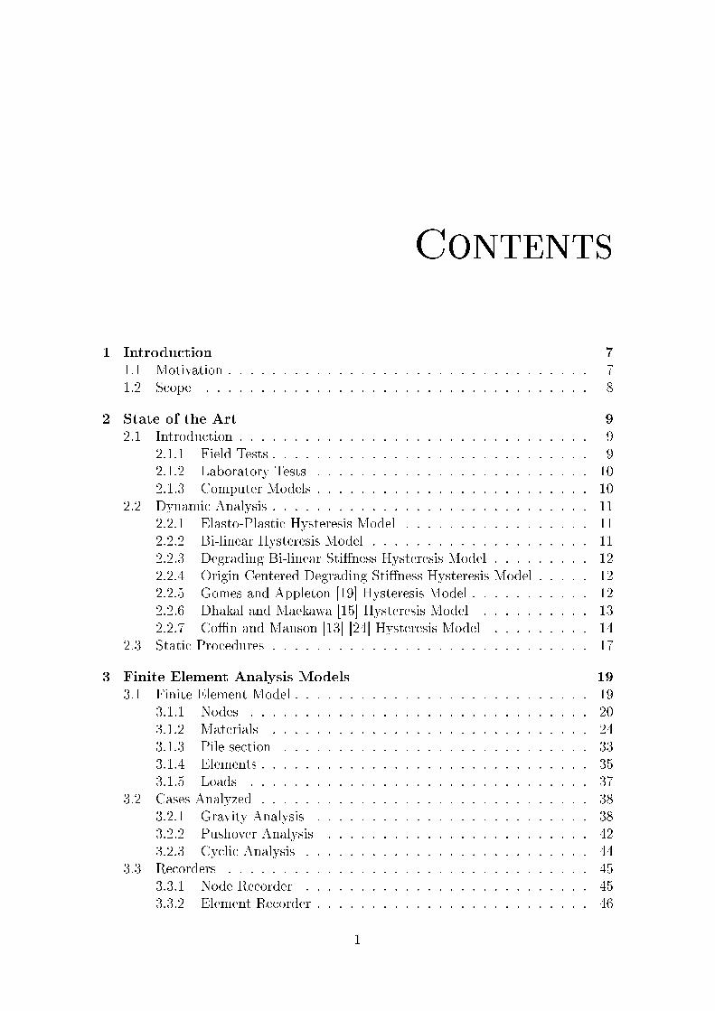
Contents
1 Introduction 7
1.1 Motivation . . . . . . . . . . . . . . . . . . . . . . . . . . . . . . . . . 71.2 Scope . . . . . . . . . . . . . . . . . . . . . . . . . . . . . . . . . . . 8
2 State of the Art 9
2.1 Introduction . . . . . . . . . . . . . . . . . . . . . . . . . . . . . . . . 92.1.1 Field Tests . . . . . . . . . . . . . . . . . . . . . . . . . . . . . 92.1.2 Laboratory Tests . . . . . . . . . . . . . . . . . . . . . . . . . 102.1.3 Computer Models . . . . . . . . . . . . . . . . . . . . . . . . . 10
2.2 Dynamic Analysis . . . . . . . . . . . . . . . . . . . . . . . . . . . . . 112.2.1 Elasto-Plastic Hysteresis Model . . . . . . . . . . . . . . . . . 112.2.2 Bi-linear Hysteresis Model . . . . . . . . . . . . . . . . . . . . 112.2.3 Degrading Bi-linear Sti�ness Hysteresis Model . . . . . . . . . 122.2.4 Origin Centered Degrading Sti�ness Hysteresis Model . . . . . 122.2.5 Gomes and Appleton [19] Hysteresis Model . . . . . . . . . . . 122.2.6 Dhakal and Maekawa [15] Hysteresis Model . . . . . . . . . . 132.2.7 Co�n and Manson [13] [24] Hysteresis Model . . . . . . . . . 14
2.3 Static Procedures . . . . . . . . . . . . . . . . . . . . . . . . . . . . . 17
3 Finite Element Analysis Models 19
3.1 Finite Element Model . . . . . . . . . . . . . . . . . . . . . . . . . . . 193.1.1 Nodes . . . . . . . . . . . . . . . . . . . . . . . . . . . . . . . 203.1.2 Materials . . . . . . . . . . . . . . . . . . . . . . . . . . . . . 243.1.3 Pile section . . . . . . . . . . . . . . . . . . . . . . . . . . . . 333.1.4 Elements . . . . . . . . . . . . . . . . . . . . . . . . . . . . . . 353.1.5 Loads . . . . . . . . . . . . . . . . . . . . . . . . . . . . . . . 37
3.2 Cases Analyzed . . . . . . . . . . . . . . . . . . . . . . . . . . . . . . 383.2.1 Gravity Analysis . . . . . . . . . . . . . . . . . . . . . . . . . 383.2.2 Pushover Analysis . . . . . . . . . . . . . . . . . . . . . . . . 423.2.3 Cyclic Analysis . . . . . . . . . . . . . . . . . . . . . . . . . . 44
3.3 Recorders . . . . . . . . . . . . . . . . . . . . . . . . . . . . . . . . . 453.3.1 Node Recorder . . . . . . . . . . . . . . . . . . . . . . . . . . 453.3.2 Element Recorder . . . . . . . . . . . . . . . . . . . . . . . . . 46
1
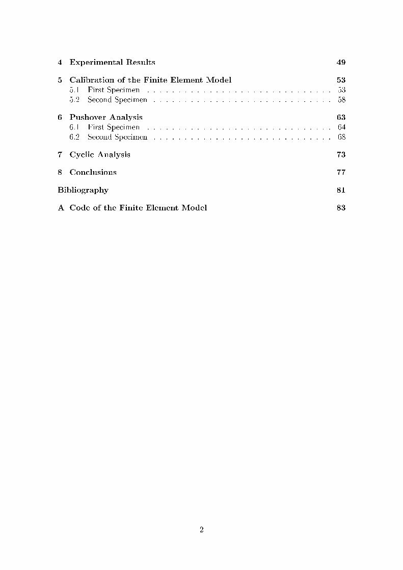
4 Experimental Results 49
5 Calibration of the Finite Element Model 53
5.1 First Specimen . . . . . . . . . . . . . . . . . . . . . . . . . . . . . . 535.2 Second Specimen . . . . . . . . . . . . . . . . . . . . . . . . . . . . . 58
6 Pushover Analysis 63
6.1 First Specimen . . . . . . . . . . . . . . . . . . . . . . . . . . . . . . 646.2 Second Specimen . . . . . . . . . . . . . . . . . . . . . . . . . . . . . 68
7 Cyclic Analysis 73
8 Conclusions 77
Bibliography 81
A Code of the Finite Element Model 83
2

List of Figures
2.1 P-y curve of sand . . . . . . . . . . . . . . . . . . . . . . . . . . . . . 112.2 Buckling parameters . . . . . . . . . . . . . . . . . . . . . . . . . . . 132.3 Slenderness . . . . . . . . . . . . . . . . . . . . . . . . . . . . . . . . 132.4 Sample parameters in the Gomes and Appleton hysteresis model . . . 142.5 Sample parameters in the Dhakal and Maekawa hysteresis model . . . 142.6 Co�n Manson Constant . . . . . . . . . . . . . . . . . . . . . . . . . 152.7 Half cycle terms . . . . . . . . . . . . . . . . . . . . . . . . . . . . . . 152.8 Strength reduction . . . . . . . . . . . . . . . . . . . . . . . . . . . . 162.9 Sample parameters in the Co�n and Manson hysteresis model . . . . 17
3.1 3D pile cap . . . . . . . . . . . . . . . . . . . . . . . . . . . . . . . . 203.2 Pile cap, elevation (left) and plan (right) . . . . . . . . . . . . . . . . 213.3 Blueprint of the soil springs . . . . . . . . . . . . . . . . . . . . . . . 223.4 Material Constants . . . . . . . . . . . . . . . . . . . . . . . . . . . . 253.5 Material Constants . . . . . . . . . . . . . . . . . . . . . . . . . . . . 263.6 Concrete con�nation . . . . . . . . . . . . . . . . . . . . . . . . . . . 263.7 Coe�cients as afunction of pf ϕ . . . . . . . . . . . . . . . . . . . . . 293.8 Relative density, % . . . . . . . . . . . . . . . . . . . . . . . . . . . . 303.9 Material Constants . . . . . . . . . . . . . . . . . . . . . . . . . . . . 323.10 Pile section . . . . . . . . . . . . . . . . . . . . . . . . . . . . . . . . 333.11 Local axis . . . . . . . . . . . . . . . . . . . . . . . . . . . . . . . . . 34
4.1 Hysteresis loop of the �rst specimen . . . . . . . . . . . . . . . . . . . 504.2 Hysteresis loop of the second specimen . . . . . . . . . . . . . . . . . 514.3 Failure of the �rst specimen . . . . . . . . . . . . . . . . . . . . . . . 514.4 Failure of the second specimen . . . . . . . . . . . . . . . . . . . . . . 52
5.1 Skeleton curve . . . . . . . . . . . . . . . . . . . . . . . . . . . . . . . 545.2 Di�erence between a single pile and a group of piles . . . . . . . . . . 555.3 x parameter calibration . . . . . . . . . . . . . . . . . . . . . . . . . . 575.4 Cd parameter calibration . . . . . . . . . . . . . . . . . . . . . . . . . 585.5 Skeleton curve . . . . . . . . . . . . . . . . . . . . . . . . . . . . . . . 585.6 x parameter calibration . . . . . . . . . . . . . . . . . . . . . . . . . . 59
3
5.7 Cd parameter calibration . . . . . . . . . . . . . . . . . . . . . . . . . 61
6.1 Position of the �rst and second pile on the pile cap . . . . . . . . . . 636.2 Position of the analysis time steps . . . . . . . . . . . . . . . . . . . . 646.3 Curvature of the pile (all analysis time steps) . . . . . . . . . . . . . 656.4 Curvature of the pile (eight analysis time steps) . . . . . . . . . . . . 656.5 Moment of the pile (all analysis time steps) . . . . . . . . . . . . . . 666.6 Position of the axail analysis time steps . . . . . . . . . . . . . . . . . 676.7 Axial load pile-soil . . . . . . . . . . . . . . . . . . . . . . . . . . . . 676.8 Node max displacement . . . . . . . . . . . . . . . . . . . . . . . . . 686.9 Position of the analysis time steps . . . . . . . . . . . . . . . . . . . . 696.10 Curvature of the pile (all analysis time steps) . . . . . . . . . . . . . 696.11 Curvature of the pile (eight analysis time steps) . . . . . . . . . . . . 706.12 Moment of the pile (all analysis time steps) . . . . . . . . . . . . . . 706.13 Position of the axial loads analysis times . . . . . . . . . . . . . . . . 706.14 Axial load pile-soil . . . . . . . . . . . . . . . . . . . . . . . . . . . . 716.15 Node max displacement . . . . . . . . . . . . . . . . . . . . . . . . . 71
7.1 Comparison of the hysteresis loop of the model with the experimentaldata. First specimen . . . . . . . . . . . . . . . . . . . . . . . . . . . 74
7.2 Comparison of the hysteresis loop of the model with the experimentaldata. Second specimen . . . . . . . . . . . . . . . . . . . . . . . . . . 75
7.3 Comparison of the hysteresis loops of �rst and the second model . . . 75
4
List of Tables
4.1 Cyclic pushover analysis . . . . . . . . . . . . . . . . . . . . . . . . . 50
5.1 Mechanical characteristics of soil . . . . . . . . . . . . . . . . . . . . 535.2 Mechanical characteristics of soil . . . . . . . . . . . . . . . . . . . . 565.3 Mechanical characteristics of soil . . . . . . . . . . . . . . . . . . . . 60
5

6

1
Introduction
1.1 Motivation
For centuries the collapse of structures under seismic loads have been occurring, butas seismic events cannot be easily predicted and are not everyday occurrences, ithas not always been an important subject of research in the �eld of engineering.In the last century the study of how and why structures collapse �rst began togain momentum and it was not very long ago that the �rst articles on the subjectbegan to appear. Even today this topic is an issue that poses many problems forthe engineering world. Speci�cally, the soil-structure interaction caused by dynamicforces, as it a topic that is still being studied and is not yet very well understood.
It has always been assumed that the response of buildings is elastic. But thisis not necessary true, if a large seismic event takes place, the buildings that ita�ects can be severely damaged. This damage is due to the displacement caused ondi�erent parts of the buildings, and this displacement is caused because of the needto dissipate the energy that the earthquake frees.
To simplify the calculations, foundations are assumed to be rigid, which makescalculated forces greater than they are in the reality. As foundations are not com-pletely rigid, they will lead to a displacement at the base of the columns that hasnot been predicted, potentially making the building fall.
This is the reason why the soil-structure interaction is so important to under-stand what the displacement would be at the base of the building. Soil-structureinteraction is the basis of how to make the structures more e�cient under dynamicloads.
The main objective of this report is to model a �nite element bridge pile capfoundation already built and test in the laboratory using OpenSees and to be ableto recognize the di�erent failure points along them, so that the behavior of similarpile caps can be predicted. Those failure points will create plastic hinges that willnot share any moment to the rest of the structure. Learning and understanding thecapacity of horizontal deformation of these piles will help us to advance the creation
7

of safer and better executed structures. If the plastic hinges are not formed, thewhole pile over the ground level will have to withstand a moment bigger than whatit has been created for, resulting in a probable failure of the entire structure.
To be able to write this report I joined Professor Aijun Ye's group of students,speci�cally the master candidate Xiaowei Wang and PhD candidate Dr He, in theirwork on seismic behavior of pile cap foundations of bridges at Tongji University. Toget familiar with their research in this �eld I helped the team build several pile capmodels with a scale 1:1 for use in their experiments. The di�erence between theirpile caps and the pile caps I used in my model was essentially the number of piles;theirs used six piles per pile cap while mine only used four. I stayed with themthroughout the process of making and testing four full models, three of which werecompletely identical whereas the height of the fourth was di�erent. While I wasassisting them I learned how to use OpenSees, create models with its code language,and program di�erent analyses; analyses that I later used to observe the failuremechanism of the piles when they are subjected to a lateral load.
1.2 Scope
The structure of this report is as follows:In the chapter 2, the state of the art describes the history on the studies of this
topic.Chapter 3 gives an explanation of how the computer model is built using OpenSees,
the geometry of the nodes, the materials, and the sections used. It also providessome analyses completed in the model (gravity, pushover and cyclic analysis), andthe recorders used along the height of the piles.
Chapter 4 describes the experimental results obtained by the 1:1 scale pile capmodels carried out by Deming Zhang under the supervision of Dr Ye Aijun at TongjiUniversity.
Chapter 5 explains the calibration of the �nite element pile cap foundation modelusing the experimental results explained in the previous chapter.
Chapter 6 discusses the pushover analysis performed in the pile cap �nite elementmodel. It gives an explanation of the di�erent failure points along the height of thepile cap, along with the forces developed in the piles at di�erent times of the analysis.
Chapter 7 is the cyclic analysis, this analysis was not able to be completed as itwill be explained in the chapter.
Chapter 8 summarizes the conclusions obtained from the overall report.
8

2
State of the Art
2.1 Introduction
Throughout the last decades, questions about how to approach the topic of dynamicanalysis have been made. The California Seismic Safety Commission [3] (1996) wasthe �rst to come up with nonlinear static procedures (capacity curve) that try torepresent what happens in seismic events, instead of using the dynamic analysis.
The capacity curve plots this placement versus the force that can be taken by anystructure. As the load and the displacement increases, di�erent part of the structurewill yield and deform inelastically, giving the engineer the necessary knowledge ofhow the building is going to fail.
Particularly for the foundations, there are three di�erent approaches that can betaken to address this topic:
• Field tests;
• Laboratory tests;
• Computer models;
2.1.1 Field Tests
Field test are one of the possible researches that can be done in order to attemptto reproduce what actually happens to the pile caps of the structures during earth-quakes and how their structural behavior can be made more e�cient.
Earthquake reports, like the one made after the Loma earthquake by the Depart-ment of California Highway Patrol [21] help scientists understand how earthquakescan a�ect the piles.
H. Matlock et al [26] made several �eld tests in di�erent groups of piles in softclay. They tested a group of 5 piles, another one of 10 piles, as well as single piles.The tests performed were both static and cyclic. For the cyclic tests, in the group of
9

10 piles the de�ections were considerably higher than for a single pile. In the 5 pilegroup however, the de�ections were similar to the single piles. Also, it was foundthat clay soils have a highly inelastic response, making it hard to use an elasticinteraction.
2.1.2 Laboratory Tests
In order to simplify the �eld tests, the laboratory tests are done by making di�erentassumptions in the composition of the soil. Over these tests several problems werestudied separately. These problems were: the e�ect of the number of piles in thebehavior of the pile cap, and the e�ect of the soil composition in its interaction withthe piles.
The e�ect of the number of piles on each pile cap has been studied widely. D. A.Brown et al [7] built separately a group of piles and a single pile, subjecting them tothe same loading in order to observe the di�erence between the forces over them. Itwas found that the number of piles makes them lose e�ciency compared to a singlepile. This is due to the shadowing e�ect, which is the decrease of soil resistance ofthe piles that is in the direction of the load.
Later on, Ernest Naesgaard [34] analyzed di�erent single piles to its lateral defor-mation. The results showed that the strongest piles could achieve a greater lateraldeformation before its failure.
Lymon C. Reese et al [22] give advice on procedures of how to design singleor pile groups, and the considerations that need to be taken into account for thereduction of the soil strength if a pile group is being used.
R. Boulanger et al [5] performed a nonlinear analysis method studying the soil-pile-structure interaction under seismic tests. These tests consisted of nine di�erentearthquakes with pike soil accelerations between 0.02g to 0.7g, and were done to twodi�erent single supported piles embedded in clay. The results obtained were thatthe p-y analysis method presented a suitable result when modeling seismic soil-pileinteraction.
The p-y curves are a widely chosen option by a lot of researcher in order torepresent the soil-structure interaction. They relate the force of the soil with itsdisplacement. The �gure 2.1 is an example of the shape of these curves.
2.1.3 Computer Models
The last option to study this problem is to build a computer model using variousprograms. There are many di�erent programs that allow the user to build a �niteelement model and perform a static or dynamic analysis.
Zhaohui Yang et al [37] made a pile cap model using OpenSees, performing withit a pushover analysis. This pushover analysis was done to 3x3 and 4x3 group pilespecimens, recording the bending moment of each of the piles. This response wasafterward compared with the results of experimental tests.
Behrouz Asgarian et al [2] made a pushover numerical analysis of di�erent speci-mens, taking into account the soil-pile interaction. This pushover numerical analysiswas made in the software "DRAIN-3DX" by making two-dimensional models. The
10

Figure 2.1: P-y curve of sand
piles of these models are head �xed at the soil height underneath the mud. Theresults show that the nonlinear �ber piles forces �t those ones in reality.
Ahmed Elgamal et al [18] also made a model in OpenSees, using a single idealpile embedded in clay. The model was done in a 3D environment with �nite elementsand then compared with 3x3 pile cap results, being able to calculate the e�ciencyof the pile group.
2.2 Dynamic Analysis
Dynamic analysis tries to reproduce exactly what happens in reality when a structureis subjected to any excitation. One common way is by introducing the hysteresisloop concept. It consists of a series of cycles of loading and unloading that representthe dynamic performance of the structural member that is being studied.
There are several models of hysteresis loops that try explain what actually hap-pens, each of them face di�erent problems that come up when trying to understandthe di�erent member behavior. From the most basic, to the ones that need to becalibrated by the parameters proposed by the authors.
2.2.1 Elasto-Plastic Hysteresis Model
This is the simplest hysteresis model that exists. It does not show any sti�ness afteryield occurs. The equation that de�nes the de�ection is 2.1.
δ =F
k0(2.1)
Before the yield occurs, and once the force achieves the yielding value of the steelFy, the displacement will continue without any change in the force.
2.2.2 Bi-linear Hysteresis Model
This model adds a small sti�ness after the yield occurs. This sti�ness is a fractionof the elastic sti�ness before the yield point.
11

Before the yield occurs this model uses the same equation of the Elasto-Plasticmodel (equation 2.1) and after it, the model behaves as the equation 2.2.
δ =F
rk0(2.2)
Where:
0 < r < 1 (2.3)
Both, the Elasto-Plastic and the Bi-linear models are not really used for researchbut they help us understand what exactly the hysteresis loop is, before starting toanalyze it in a more complex way.
2.2.3 Degrading Bi-linear Sti�ness Hysteresis Model
This model changes the sti�ness of the structural member with each new cycle. Theratio of change in sti�ness is shown in the equation 2.4.
ki = k0(dydm
)α (2.4)
Where:dy displacement at the yield pointdm displacement when the second cycle reaches the yield point
2.2.4 Origin Centered Degrading Sti�ness Hysteresis Model
The sti�ness of this model degrades gradually but it always goes through the centerof the axis (the zero). The problem of this model is that it shows very little energydissipation.
2.2.5 Gomes and Appleton [19] Hysteresis Model
This is one of the options that OpenSees gives in order to model the hysteresis in areinforced concrete member.
Figure 2.2 displays the di�erent buckling coe�cients from [19]. Those parametersare:
• β is an ampli�cation factor, it calibrates and adjusts the buckling curve;
• r factor mainly adjusts the desired curve between the buckled curve and theunbuckled curve. The factor ranges from 0.0 to 1.0;
• γ is the positive stress location about which the buckling factor is initiated;
Also another parameter that needs to be de�ned is the slenderness of the steel-baras it is shown in the �gure 2.3, the slenderness will be:
ISR =Ludb
(2.5)
12
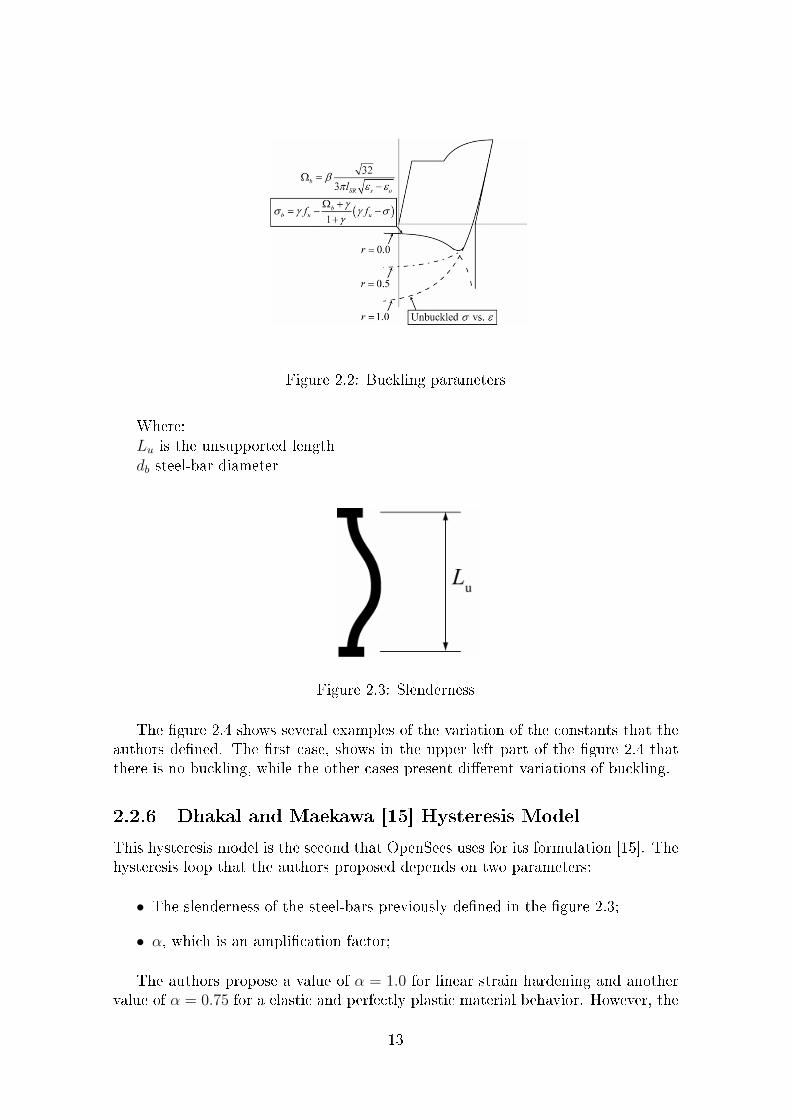
Figure 2.2: Buckling parameters
Where:Lu is the unsupported lengthdb steel-bar diameter
Figure 2.3: Slenderness
The �gure 2.4 shows several examples of the variation of the constants that theauthors de�ned. The �rst case, shows in the upper left part of the �gure 2.4 thatthere is no buckling, while the other cases present di�erent variations of buckling.
2.2.6 Dhakal and Maekawa [15] Hysteresis Model
This hysteresis model is the second that OpenSees uses for its formulation [15]. Thehysteresis loop that the authors proposed depends on two parameters:
• The slenderness of the steel-bars previously de�ned in the �gure 2.3;
• α, which is an ampli�cation factor;
The authors propose a value of α = 1.0 for linear strain hardening and anothervalue of α = 0.75 for a elastic and perfectly plastic material behavior. However, the
13

Figure 2.4: Sample parameters in the Gomes and Appleton hysteresis model
materials usually are none of the cases related before, although a value of α = 1.0is usually used when it is assumed that the material has strain hardening.
The �gure 2.5 displays both cases, when buckling appears (right of the �gure),and when there is no buckling (left of the �gure).
Figure 2.5: Sample parameters in the Dhakal and Maekawa hysteresis model
2.2.7 Co�n and Manson [13] [24] Hysteresis Model
This is the third and last hysteresis model that OpenSees uses. This model takesinto account the strength degradation of each cycle ([13] [24]). The authors proposedthree di�erent parameters in order to calibrate the hysteresis loop. These parametersare α, Cf and Cd.
14

The three of them together represent the fatigue of the steel.The number of half cycles until the fracture of the half cycle plastic strain am-
plitude can be related using α and Cf , as shown in this �gure 2.6:
Figure 2.6: Co�n Manson Constant
The total half cycle strain amplitude, εt, is shown in the �gure 2.7. It is thechange in strain.
Figure 2.7: Half cycle terms
These are the equations:
εp = εi −σiEs
(2.6)
D = Σ(∆εpCf
)1α (2.7)
The cumulative damage factor is zero at no damage and 1.0 at fracture. Once abar has been determined to have fractured, the strength is rapidly degraded to zero.
There is a degradation constant that will be used to de�ne the strength lossthat results in a softening of the material. There are several possible relationshipsbetween the degradation constant and the de�ection, this is a linear relationshipbetween both of them:
φSR = K1D (2.8)
But this relation can be written so that the strength degradation is independentof the numbers of half cycles until failure. The calibration is easier to do if both the
15

Figure 2.8: Strength reduction
number of cycles until failure and the strength degradation are not related. This isanother equation using Cd as the strength.
φSR = Σ(∆εpCd
)1α (2.9)
The next equation is the relation between Cd and K1 (both degradation con-stants):
Cd =CfKα
1
(2.10)
There are some suggested values to start with; these values are explained in [8].Although an additional calibration may be done in order to adjust the behavior ofthe modeled reinforced steel to the real behavior of this steel.
α = 0.506Cf = 0.26Cd = 0.389Sample Simulations of Degradation behavior that depends on the value of the
parameters can be seen in the �gure 2.9.α is best obtained from calibration of test results. α is used to relate damage
from one strain range to an equivalent damage at another strain range. This isusually constant for a material type.
Cf is the ductility constant used to adjust the number of cycles to failure. Ahigher value for Cf will result in a lower damage for each cycle. A higher value Cftranslates to a larger number of cycles to failure.
Cd is the strength reduction constant. A larger value for Cd will result in alower reduction of strength for each cycle. The four charts shown in the �gure 2.9demonstrate the e�ect that some of the variables have on the cyclic response.
The upper left example of the �gure 2.9 has no strength degradation with eachcycle. This is due to having a value of Cd = 0. The one on its right displays astrength degradation based on the values that it shows, however, if the value of Cdis changed to be 0.6, the response of the model will change as it can be seen in thelower left part of the �gure. Finally, if Cd is returned to its suggested value, butinstead Cf is changed to 0.15, the accumulation of damaged will increase makingthe bar failing before, even presenting the same strength reduction.
16

Figure 2.9: Sample parameters in the Co�n and Manson hysteresis model
2.3 Static Procedures
The study of dynamic analysis using nonlinear static procedures (like a pushoveranalysis or capacity analysis) is a problem that has previously been faced. The �rstguideline on the subject was written by the California Seismic Commission [3] in1996. The purpose of this analysis is to recreate the inelastic behavior that occursin the structures when submitted to a ground motion acceleration. As previouslystated, even if the structures are assumed to be elastic and the foundations rigid, thisis not true as the structures can show inelastic behavior under seismic events andthe foundations are partially �exible, admitting a small displacement. This groundmotion acceleration causes a displacement in the foundation of the structures.
With this method, engineers can actually know how the structure fails, andwhich parts are going to yield �rst. The result of this analysis is a comparison ofthe displacement produced with the forced applied, called the capacity curve (orpushover curve).
Balram Gupta et al [20] studied this problem and proposed a spectra for apushover. Then they compared it with the inelastic analysis in order to see theaccuracy of the pushover spectra proposed. It was seen that the pushover spectracan represent the most important attributes of the analysis (failure mechanism anddrift) in di�erent kinds of structures, making nonlinear static analysis reliable.
Another advantage of this procedure versus the dynamic procedure, is the re-duction of the computational demand while still performing an accurate estimationif certain conditions are assumed.
17

18

3
Finite Element
Analysis Models
3.1 Finite Element Model
The model consists of a square pile cap foundation of 1 m for each cross section anda height of 0.4 m. It also have four piles divided in a 2x2 symmetric pattern witha 0.15 m square meter section for each one of the four piles. The center of thesepiles will be separated by each other with a distance of 0.45 m, as is illustrated inthe �gures below. The length of the piles are 4.5 m from top to bottom but with3.7 m of them under the ground level, meaning that above this level remain a pilelength of 0.8 m that is not embedded. The ground of this pile cap foundation willbe formed by sand, with its particular speci�cations found later in this report.
The dimensions of this model have been determined so that it can be calibratedwith the experimental tests that have already been carried out in the report 'Ex-perimental study on seismic performance of elevated pile-cap foundation of bridges'([14]) done by Master degree student Deming Zhang of Tongji University. This ex-periment was conducted under the supervision of his professor, Aijun YE, in thelaboratory facilities that Tongji University has at its Siping campus.
Once calibrated, a failure mechanic analysis will be done on this model in orderto obtain exactly how the structure fails.
For building the model the �rst thing that needs to be done is to de�ne thedimensions of the pile cap foundation and the degrees of freedom of each node. Thismodel is three dimensional with six degrees of freedom for each one of the nodes ofthe structure. The units of measurements that will be used are: tons, kilo newtons,and meters.
A model design in OpenSees (Open System for Earthquake Engineering Simu-
19

Figure 3.1: 3D pile cap
lation [28]) needs a series of commands in order to build the structure as wanted.These commands will be explained one by one with the formulation behind themand what is their purpose ([27]). The procedure will be to:
• De�ne the nodes (coordinates, mass and constraints);
• De�ne the materials that are going to be used;
• De�ne the section of the elements;
• De�ne the element that will represent the di�erent part of the model;
• De�ne the loads;
After all these steps are �nished, the pile cap foundation will be completely builtand the di�erent analyses of the model can commence. The �gure 3.2 is a layout ofhow the pile cap and the piles are.
And a sketch of how the springs will be attached to the piles is shown in the�gure 3.3.
3.1.1 Nodes
The nodes are the �rst item to be designed in the code of OpenSees. The inputsthat they need are the coordinates, mass and constraints. While not all the nodesneed to be constrained or have mass, they do need to have coordinates.
20

Figure 3.2: Pile cap, elevation (left) and plan (right)
3.1.1.1 Coordinates
For obtaining the node coordinates in OpenSees, the only thing that is needed beforeprogramming them is to know the discretization that is wanted for the model. Afterthis, they can be obtained using the following command:
node $nodeTag $coords
$nodeTag: node identifying number
$coords: nodal coordinates X Y Z
# pile 1
for {set i 1} {$i <= 46} {incr i 1} {
node $i [expr $bx] [expr $by] [expr (-38+$i)*0.1]
}
This is the code that generates the nodes of the �rst pile, only the pile nodes(bx and by are the length from the center of the pile cap to the center of the pile,in both x and y direction).
The distance between the nodes considered here is 0.1 m. That means that ineach pile there will be 46 nodes from the bottom to the top of the piles above groundlevel (4.5 m), and in the soil there will be 38 nodes from the bottom of the pilesuntil the ground level (3.7 m).
Both the pile and the soil nodes will share the same coordinates for each one ofthe piles that are under the ground level.
21

Figure 3.3: Blueprint of the soil springs
22
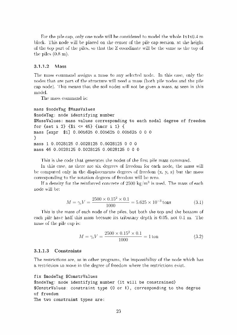
For the pile cap, only one node will be considered to model the whole 1x1x0.4 mblock. This node will be placed on the center of the pile cap section, at the heightof the top part of the piles, so that the Z coordinate will be the same as the top ofthe piles (0.8 m).
3.1.1.2 Mass
The mass command assigns a mass to any selected node. In this case, only thenodes that are part of the structure will need a mass (both pile nodes and the pilecap node). This means that the soil nodes will not be given a mass, as seen in thismodel.
The mass command is:
mass $nodeTag $MassValues
$nodeTag: node identifying number
$MassValues: mass values corresponding to each nodal degree of freedom
for {set i 2} {$i <= 45} {incr i 1} {
mass [expr $i] 0.005625 0.005625 0.005625 0 0 0
}
mass 1 0.0028125 0.0028125 0.0028125 0 0 0
mass 46 0.0028125 0.0028125 0.0028125 0 0 0
This is the code that generates the nodes of the �rst pile mass command.In this case, as there are six degrees of freedom for each node, the mass will
be computed only in the displacements degrees of freedom (x, y, z) but the masscorresponding to the rotation degrees of freedom will be zero.
If a density for the reinforced concrete of 2500 kg/m3 is used. The mass of eachnode will be:
M = γcV =2500× 0.152 × 0.1
1000= 5.625× 10⁻³ tons (3.1)
This is the mass of each node of the piles, but both the top and the bottom ofeach pile have half this mass because its tributary depth is 0.05, not 0.1 m. Themass of the pile cap is:
M = γcV =2500× 0.152 × 0.1
1000= 1 ton (3.2)
3.1.1.3 Constraints
The restrictions are, as in other programs, the impossibility of the node which hasa restriction to move in the degree of freedom where the restrictions exist.
fix $nodeTag $ConstrValues
$nodeTag: node identifying number (it will be constrained)
$ConstrValues: constraint type (0 or 1), corresponding to the degree
of freedom
The two constraint types are:
23
0 unconstrained
1 constrained
This is the code that generates the nodes of the �x command of the �rst pile soilnodes.
In this model all the soil nodes will be constrained (they are not allowed to move)from the top to the bottom. Furthermore, the bottom nodes of each pile will beconstrained in a vertical direction, not allowing it to move vertically.
3.1.2 Materials
In the process of building the pile cap foundation model three di�erent materialswere used: concrete, steel and sand (for the soil). For generating them, OpenSeeshas several commands that may be implemented, depending on the formulationbehind them that �t best the material behavior in the reality.
3.1.2.1 Steel
The section of each one of these piles has four reinforcing steel bars (one in eachcorner), and a diameter of φ12. Therefore, the area of one reinforcing steel barwould be:
As =πD2
4=π(12)2
4= 113mm2 = 1.13× (10)−4 m2 (3.3)
The stirrups are used to calculate the strength of the uncon�ned concrete andwill be de�ned later when explaining the concrete material.
The command used to model this material is ReinforcingSteel, this commandhas the following input data:
uniaxialMaterial ReinforcingSteel $matTag $fy $fu $Es $Esh $esh $eult
< -CMFatigue $Cf $alpha $Cd >(optional)
$matTag: material tag that will be used when defining the elements
$fy: yield strength of the steel
$fu: ultimate strength of the steel
$Es: initial elastic tangent of the steel
$Esh: tangent at initial hardening of the steel
$esh: strain at the initial hardening
$eult: strain at the maximum strength
CMFatigue: Coffin-Manson Fatigue and Strength Reduction, where:
$Cf: Coffin-Manson constant C
$alpha: Coffin-Manson constant alpha
$Cd: cyclic strength reduction constant
This �gure represents the values described above and how the ReinforcingSteelcommand will use them in its theory curve:
The values of the steel that were used for the test, and that are going to be usedwhen building this model, are:
24

Figure 3.4: Material Constants
fy = 310MPa (3.4)
fu = 459MPa (3.5)
Es = 1.5× (105)MPa (3.6)
Esh = 1540MPa (3.7)
esh = 0.024 (3.8)
eult = 0.15 (3.9)
These are the main values for building the material but there is also anotherparameter that has been taken into account. That would be the fatigue of the steel,which is computed into this command by saying -CMFatigue.
In the state of art the three options that OpenSees has for modeling the hysteresisof the steel are taken into account. In this report the Co�n-Manson fatigue modelwas chosen in order to get a better approach of the fatigue that appears in the steelwhen a cyclic load is applied to it.
For the beginning of the iterations the parameters were chosen as:
α = 0.506
Cf = 0.26
Cd = 0.389
Those parameters will change later in the calibration of the model in order to�t the test results, although the α for example is the same if the material does notchange. This means that it will not be changed as the steel bars are the same.
25

3.1.2.2 Concrete
For the concrete I used the OpenSees command Concrete01. This command repre-sents a zero tensile strength concrete, as is shown in the �gure 3.5.
Figure 3.5: Material Constants
There are two parts in the pile section, the con�ned and the uncon�ned parts.They di�er from each other in that the �rst is the part of the section that is sur-rounded by stirrups, while the other part is the cover. In the �gure 3.6, the di�erencebetween one and the other is apparent:
Figure 3.6: Concrete con�nation
The main reason for con�ning the concrete is the advantage that this concretehas in its ductility behavior, given by the compression of the stirrups, as well as alittle increment in the compressive strength.
To program the concrete in OpenSees the command needed is:
uniaxialMaterial Concrete01 $matTag $fpc $epsc0 $fpcu $epsU
$matTag: the material tag that will be used when defining the elements
$fpc: the compressive strength of the concrete
26

$epsc0: concrete strain at maximum compressive strength
$fpcu: concrete ultimate strength
$epsU: concrete strain at ultimate strength
The concrete used is C40, for both the con�ned and uncon�ned concrete. Thedi�erence in strength of the con�ned and uncon�ned concrete given by the stirrupscan be computed with the following formula:
k = 1 +ρsfyhf ′c
(3.10)
Where:ρs is the +transversal+ reinforcement volume ratiofyh is the yield strength of the steelf ′c is the compressive strength of the concreteThe reinforcing stirrups are:φ = 8 ; fyh = 235 MPaSo ρs:
ρs = 4π×824
1502= 8.94× 10⁻³ (3.11)
And �nally:
k = 1 +8.94× 10−3 × 410
40= 1.0916 (3.12)
Now the compressive strength of the con�ned concrete can be computed as:
f ′cc = k × f ′c (3.13)
f ′cc = 1.0916× 46 = 50.21MPa (3.14)
This is the theoretic way to calculate both strengths, but actually the experi-mental values obtained when doing the experiment were:
f ′c = 34.25MPa (3.15)
f ′cc = 41.85MPa (3.16)
And:
εcc0 = 0.0025 (3.17)
εc0 = 0.002 (3.18)
Thus, these are the input values in the Concrete01 command.In the �gure 3.5, the ultimate concrete strength is computed as:
f ′ccult = 0.4× f ′cc = 0.4× 50.21 = 20.08MPa (3.19)
27
f ′cult = 0.4× f ′c = 0.4× 46 = 18.4MPa (3.20)
And the ultimate concrete strains are:
εccult = 0.025 (3.21)
εcult = 0.006 (3.22)
3.1.2.3 Soil
For modeling the soil, the API code (2005) [1] was followed in order to computeboth the lateral bearing capacity and the displacement at 50% of the load.
This lateral bearing capacity varies with the depth at each node that is beingconsidered. There are two equations that need to be computed, because the lateralbearing capacity will be the minimum value of them. The �rst equation is:
pus = (C1H + C2D)γH (3.23)
This equation determines the lateral bearing capacity at shallow depths, whilethe next one determines this lateral bearing capacity at deeper depths.
pud = C3DγH (3.24)
Where:pu (kN/m) is the ultimate resistance of the soilH (m) is the depth at each nodeC1, C2, C3 are coe�cients that will be determined laterD (m) is the average pile diameterϕ = 31◦ is the friction angleγ = 16.1 kN/m3 is the e�ective soil weightThe lateral soil resistance-de�ection (p-y) relationships for sand are also non-
linear and in the absence of more de�nitive information may be approximated atany speci�c depth H, with the following expression:
P = Aputanh(kH
Apuy) (3.25)
Where:A = 0.9 For a cyclic loadpu kN/m ultimate bearing capacity at depth Hym is the later de�ectionk kN/m3 initial modulus of subgrade reactionBut what we need to compute is y50, not y. As it will be explained later, y50
by de�nition is the lateral soil resistance when the de�ection reaches 50% of themaximum de�ection. So:
1
2pu = Aputanh
kH
Apuy50 (3.26)
28

And solving in order to compute y50:
y50 = tanh(1
2A)ApukH
(3.27)
Having the friction angle of the sand, the three di�erent constants can be ob-tained using the next graph of the API code [1].
As said before, pu is a distributed force (depends on the length), but this isa �nite element analysis, which means that it will have to be multiplied by thetributary length of the node where it is being applied. This tributary length is 0.1meters for all the nodes excluding the ones that are in the border. These nodes willhave half that tributary length, 0.05 meters.
In this case study, as the friction angle is ϕ = 36 ◦, the three di�erent constantsare:
Figure 3.7: Coe�cients as afunction of pf ϕ
C1 = 3.1 (3.28)
C2 = 3.5 (3.29)
C3 = 55 (3.30)
As before, the friction angle is 36◦, knowing that the sand is above the watertable:
k = 160 lb/in3 = 43913.6 kN/m3 (3.31)
Also, it has to be taken into account that during the test the sand that coversthe piles will move, making a hole that surrounds the pile. This means that the
29
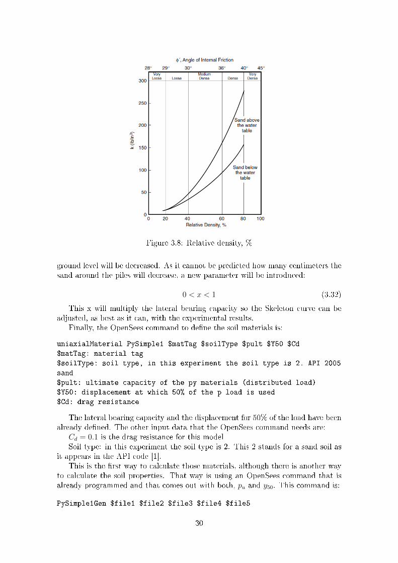
Figure 3.8: Relative density, %
ground level will be decreased. As it cannot be predicted how many centimeters thesand around the piles will decrease, a new parameter will be introduced:
0 < x < 1 (3.32)
This x will multiply the lateral bearing capacity so the Skeleton curve can beadjusted, as best as it can, with the experimental results.
Finally, the OpenSees command to de�ne the soil materials is:
uniaxialMaterial PySimple1 $matTag $soilType $pult $Y50 $Cd
$matTag: material tag
$soilType: soil type, in this experiment the soil type is 2. API 2005
sand
$pult: ultimate capacity of the py materials (distributed load)
$Y50: displacement at which 50% of the p load is used
$Cd: drag resistance
The lateral bearing capacity and the displacement for 50% of the load have beenalready de�ned. The other input data that the OpenSees command needs are:
Cd = 0.1 is the drag resistance for this modelSoil type: in this experiment the soil type is 2. This 2 stands for a sand soil as
it appears in the API code [1].This is the �rst way to calculate those materials, although there is another way
to calculate the soil properties. That way is using an OpenSees command that isalready programmed and that comes out with both, pu and y50. This command is:
PySimple1Gen $file1 $file2 $file3 $file4 $file5
30

$file1: name of the input fail that contains the soil and the pile
properties that are required to define these materials
$file2: name of the input fail that contains all the nodes that the
soil elements are going to use
$file3: name of the input fail that contains the information of the
zeroLength elements that will be assigned to the PySimple1 materials
$file4: name of the input fail that contains the information about
the column elements that define the pile
$file5: name of the output files where Opensees will print out the
PySimple1 materials data
The �le 5 has to be computed before running the model. For computing it, allthose four input �les need to be in the same folder as the model. Then, start anew window and source the �le where the PySimpleGen1 is. This will automaticallycreate the �le5. Finally, after all this is �nished, the only thing that needs to bedone is call the Pymaterials �le (�le5) doing a source in the model.
Once the �rst soil material is �nished, the implementation of the rest of thesoil materials can start. There is another soil material that will create a verticalspring between the soil and the pile nodes, this is Tz soil material. However, at thebottom of the pile the material will not be this Tz soil material because there is onlycompression. This last spring will be explained ahead. The Tz soil material will beprogrammed using the second option of the Py material (TzSimple1Gen):
TzSimple1Gen $file1 $file2 $file3 $file4 $file5
$file1: name of the input fail that contains the soil and the pile
properties that are required to define these materials
$file2: name of the input fail that contains all the nodes that the
soil elements are going to use
$file3: name of the input fail that contains the information of the
zeroLength elements that will be assigned to the TzSimple1 materials
$file4: name of the input fail that contains the information about
the column elements that define the pile
$file5: name of the output files where OpenSees will print out the
TzSimple1 materials data
The calculation of this material is the same of the Pysimple1Gen. The onlything that will change between both specimens is �le1. When de�ning this �le, theparameters of the soil (friction angle and density of the sand) will be di�erent. Also,the type of the Tz material used is 2, this means that the formulation behind it isMosher relation.
Finally, the last soil material that will be used is the Qz soil material. Thismaterial will be de�ned so that it can link the soil and the pile nodes at the bottomof the pile by using a vertical spring. The di�erence between this vertical spring andthe soil spring is that at the bottom of the pile the soil will not give any tractionforce to the pile, only compression, and this is what the Qz material does. Thecommand is QzSimple1 Material.
This command is used to construct a QzSimple1 uniaxial material object.
31

uniaxialMaterial QzSimple1 $matTag $qzType $qult $z50
$matTag: material tag.
$soilType: soil type, in this experiment the soil type is 2.
Vijayvergiya's (1977) relation for piles in sand
$qult: ultimate capacity of the qz material (distributed load)
$z50: displacement at which 50% of qult is used
Looking at Vijayvergiya's relation for piles in sand, the qult and z50 for thebottom of the pile will be:
qult = 65 kN (3.33)
z50 = 0.0027m (3.34)
3.1.2.4 Elastic material
The last material that is going to be used is an elastic material that will help laterwhen building the section of the piles. The command for this material is:
uniaxialMaterial Elastic $matTag $E
$matTag: unique material object integer tag
$E: tangent
The young modulus for this material is E = (10)10 MPa, so it is sti� enough.This is the line that represents the behavior of an elastic material:
Figure 3.9: Material Constants
32

3.1.3 Pile section
The section that is used to model the piles, as has already been said, is a squaresection of 15 centimeters on each side. It will be the same for the four piles.
The section has a cover of 2 cm surrounding the stirrups (uncon�ned concrete),and it will count with four reinforcing steel bars, each one in one corner and withan area of 1.13 ∗ (10)−4 m2 as said before. A �gure of the section is shown here:
Figure 3.10: Pile section
The section is denominated a �ber section in OpenSees because of the di�erent�bers that will compound it. Composing a section with di�erent �bers is a methodthat can be used in �nite element environments in order to calculate the plasticityof the piles. This plasticity is the result of the increment of deformation of thedi�erent �bers at each plane section along the pile length. For creating those �bersOpenSees has a couple of options where you can choose from depending on what �tbest each �ber.
For the concrete there is a speci�c command called 'patch quad' that builds aPatch object with a quadrilateral shape. The command is:
patch quad $matTag $numSubdivIJ $numSubdivJK $yI $zI $yJ $zJ $yK
$zK $yL $zL
$matTag: material tag of the previously defined UniaxialMaterial
$numSubdivIJ: subdivisions of the square in both directions of
the axis
$yI $zI: coordinates of the I corner
$yJ $zJ: coordinates of the J corner
$yK $zK: coordinates of the K corner
$yL $zL: coordinates of the L corner
This command �ts both the con�ned and uncon�ned concrete, but while thecon�ned concrete can be modeled using only one 'patch quad' command, the un-
33

con�ned concrete will need four di�erent 'patch quads' to model the four di�erentcovers of the con�ned concrete. Those four sides will be the top, left, bottom andright part that surround the stirrups.
# Create the concrete cover fibers (right, left, top, bottom)
patch quad 2 10 2 [expr -$y1] [expr $z1-$cover]
$y1 [expr $z1-$cover] $y1 $z1 [expr -$y1] $z1 ? #1
patch quad 2 10 2 [expr -$y1] [expr -$z1] $y1 [expr -$z1]
$y1 [expr $cover-$z1] [expr -$y1] [expr $cover-$z1] ? #2
patch quad 2 2 10 [expr -$y1] [expr $cover-$z1]
[expr $cover-$y1] [expr $cover-$z1] [expr $cover-$y1]
[expr $z1-$cover] [expr -$y1] [expr $z1-$cover] ? #3
patch quad 2 2 10 [expr $y1-$cover] [expr $cover-$z1]
$y1 [expr $cover-$z1] $y1 [expr $z1-$cover] [expr $y1-$cover]
[expr $z1-$cover] ? #4
This is the code for de�ning the uncon�ned concrete.
Figure 3.11: Local axis
Figure 3.11shows the local coordinates of the pile section and the di�erent num-bers of the 'patch quad' for the uncon�ned concrete.
For designing the reinforcing steel �bers the command straight layer was used.As said before, each section has four reinforcing steel bars distributed in two lines,and this command builds a straight layer of reinforcing bars. The command is:
layer straight $matTag $numBars $areaBar $yStart $zStart $yEnd $zEnd
$matTag: material tag of the previously defined UniaxialMaterial
$numBars: number of reinforcing bars on each layer
$areaBar: area of each reinforcing bar
$yStart $zStart: coordinates of the beginning point of reinforcing
layer (local coordinates)
$yEnd $zEnd: coordinates of the ending point of reinforcing layer
(local coordinates)
34

For building the four reinforcing steel bars, two layer straight command need tobe done. Both starting in the same reinforcing steel bar, but ending in the otherbars that are in other directions. The program, when reading this, will understandthat it has to build a square mesh of two reinforcing bars per side.
Once the di�erent �ber sections are de�ned, this section can be used in any ofthe elements to give them a cross section (although a section aggregator commandneeds to be called in order to join both the element and the section together). Thiscommand is:
section Aggregator $secTag $matTag1 $string1 -section $sectionTag
$secTag: section tag
$matTag1: uniaxial material previously defined
$string1: represent the force deformation corresponding to each
section. One of the following strings should be picked:
P Axial force-deformation
Mz Moment-curvature about section local z-axis
Vy Shear force-deformation along section local y-axis
My Moment-curvature about section local y-axis
Vz Shear force-deformation along section local z-axis
T Torsion Force-Deformation
-section $sectionTag: section already defined to which the
uniaxialMaterial will be added
There are two di�erent ways to use the section aggregator, it can create a newsection for itself, or use an already created section to add it to a material thatrepresents any load. In this case the second option is chosen. The material isalready created (elastic) and the section too (�ber section), and by adding the Tstring, we represent the torsion of this section.
3.1.4 Elements
OpenSees provides us with a wide range of possibilities when about to choose el-ements. Depending on the element which will try to represent reality, one or theother command would be chosen.
It also has to be taken into account the position of the element in the global co-ordinates. At the beginning of the report, a �gure explaining the global coordinatesused for building this model appeared. Now, for each one of the elements, thereis a transformation vector that changes the axis from the local coordinates (of theelement) to the global coordinates (previously de�ned). This vector is called thegeometric linear transformation vector, and it is programmed like this:
geomTransf Linear $transfTag $vecxzX $vecxzY $vecxzZ
$transfTag: transformation tag
$vecxzX $vecxzY $vecxzZ: transformation vector
Firstly, the design of the piles would be done by using a nonlinear element called'dispBeamColumn'. This is as follows:
35
element dispBeamColumn $eleTag $iNode $jNode $numIntgrPts $secTag
$transfTag
$eleTag: element tag
$iNode $jNode: beginning and end nodes of the element
$numIntgrPts: number of points that are going to be integrated along
the element
$secTag: section tag of the element
$transfTag: coordinate transformation vector
The integration along the element is based on the Gauss-Legendre quadrature.The next element that is going to be used is the 'elasticBeamColumn'. This
element is used to join the top of each pile with the pile cap node at its center. Asthese elements are vertical, the transformation vector should be (1 0 0).
element elasticBeamColumn $eleTag $iNode $jNode $A $E $G $J $Iy $Iz
$transfTag
$eleTag: element tag
$iNode $jNode: beginning and end nodes
$A: section area of the element
$E: young's Modulus
$G: shear Modulus
$J: torsional moment of inertia of its section
$Iz: second moment of area about the local z-axis
$Iy: second moment of area about the local y-axis
$transfTag: coordinate transformation vector
As this element tries to represent the pile cap, its stiffness has to
be greater than the pile elements.
As these elements are horizontal the transformation vector should be
(0 0 1).
Finally, the elements that are used to connect the soil with the pile elements arecalled 'zeroLength' elements. The reason of this name is because the coordinates ofthese pile and soil nodes are the same, so the length of the elements necessary hasto be zero.
The command to program this element is:
element zeroLength $eleTag $iNode $jNode -mat $matTag1 $dir $dir
$eleTag: element tag
$iNode $jNode: beginning and end nodes of the element
-mat $matTag: tag associated with a uniaxialMaterial previously defined
$dir $dir: uniaxialMaterial direction
The material for the matTag will change with the depth as, has already beenexplained when de�ning the soil material.
Also, as there is no length in these elements, the direction of the p-y materialhas to be given. This direction goes along the �rst axis (x), and as this is the �rstdirection, the input would be 1.
36

3.1.5 Loads
There are three loads that are going to be applied to this structure, the gravity load,the pushover load and the cyclic load. At this moment, only the consideration ofthe gravity loads will be taken into account. The pushover load and how to performthe pushover analysis will be explained later on.
In OpenSees, gravity loads require two di�erent steps. Firstly, a load patternhas to be called. Then, the gravity loads will have to be added to this pattern, sowhen applying the pattern the gravity loads will be put with it.
Furthermore, for de�ning the pattern, a time series command will have to bedone. What this command does, is create a LinearSeries (TimeSeries) object thatwill be associated with the LoadPattern de�ned ahead. This command is:
Linear <-factor $cFactor>
$cFactor: this factor is optional and would be taken as 1 if missing
(default)
The factor will a�ect the linear time series.The next step is to de�ne the load. As this is a �nite element analysis the gravity
loads of the elements will be, indeed, point loads applied at the nodes. Those nodeswill be the same nodes that already have a mass, and for computing their load theonly thing that needs to be done is to multiply that mass (in tons) for the gravityacceleration, getting the load in kilo newtons. The command is:
load $nodeTag $LoadValues
$nodeTag: node where the load is applied
$LoadValues: value of the load at that node in each degree of freedom
The last step is to de�ne the load pattern. The loads can be directly de�ned atthe same time as the load pattern.
pattern Plain $patternTag (TimeSeriesType arguments) {
load $nodeTag $LoadValues
}
$patternTag: identifying tag of the pattern
TimeSeriesType arguments: the TimeSeries object previously defined
$nodeTag: node where the load will be applied
$LoadValues: value of the load at that node in each degree of freedom
This is the code use to build the loads for the first pile. As the
loads are gravity loads, they are only applied in the third degree of
freedom (Z) with a minus sign.
pattern Plain 1 "Linear" {
# pile 1
for {set k 2} {$k <= 45} {incr k 1} {
load $k 0 0 -0.055125 0 0 0
}
37
load 1 0 0 -0.0275625 0 0 0
load 46 0 0 -0.0275625 0 0 0
}
3.2 Cases Analyzed
Once the model is already �nished, it means that the analysis can start to be per-formed. There are di�erent kinds of analysis that can be done, depending on thepurpose of the study. In this case, the analyses that are going to be studied are:
• Gravity analysis;
• Pushover analysis;
• Cyclic analysis;
3.2.1 Gravity Analysis
The gravity analysis consists of the following series of commands. These commandsare:
• Constraint;
• Numberer;
• System;
• Test;
• Algorithm;
• Integrator;
• Analysis;
Constraint: This is the �rst command that has to be implemented. It is used tobuild the ConstraintHandler object which determines the way to use the constraintequations during the analysis. Constraint equations will make a speci�c value coin-cide for a DOF, or a relationship between DOFs. These degrees of freedom can bebroken down into Ur (retained DOF's), and Uc (the condensed DOF's), getting:
X =
(Ur
Uc
)(3.35)
The kind of constraint command that is going to be used is the Transformationconstraint. It will make the constraints use the transformation method (shownbelow). Its main purpose is to condense the constrained DOF's, by reducing thesize of the system. It is the recommended method for a transient analysis. Thecommand is:
38

constraints Transformation
The constraint equation takes the following form:
(T′KT)Ur = T′R (3.36)
Numberer: This is next command. It is used to build the DOF Numberer object,which determines how the degrees of freedom are numbered.
The numberer command used here is RCM. RCM assign nodes to degrees offreedom using the Reverse Cuthill-McKee algorithm. The RCM algorithm orderingis frequently used when a matrix needs to be generated whose rows and columns arenumbered according to the numbering of the nodes. If the renumbering of the nodesis appropriate, a much smaller bandwidth matrix can be produced. This picture isan example about how the algorithm works, reducing considerably the number ofcalculations that the program will perform.
The command that needs to be written is:
numberer RCM
System: Then, the following step is the solving of the system. The system com-mand is used to build the two objects that will save and solve the system equationsin the analysis, these objects are the LinearSOE and LinearSolver.
Inside this command, the system that is going to be used is the BandGeneralsystem. The command input is:
system BandGeneral
Test: Now, the test command will be explained. The purpose of this command isto build a ConvergenceTest object. When performing a SolutionAlgorithm objectthe convergence needs to be checked and compared with a determined value. Thisconvergence is applied to the following equation:
K = R (3.37)
This command is used to construct a CTestNormDispIncr object which testspositive force convergence if the 2-norm of the x vector (the displacement increment)in the LinearSOE object is less than the speci�ed tolerance.
test NormDispIncr $tol $maxNumIter
$tol: tolerance at which it has already converge enough
$maxNumIter: maximum number of iterations that will be done at each
step
The equation that needs to be satis�ed when using this command is:
2√δUTδU < tol (3.38)
39

Algorithm: This command will build the SolutionAlgorithm object that has justbeen mentioned in the test command. This object will select the di�erent steps thatare going to be followed in order to solve the nonlinear equation.
The subcommand used for the algorithm is Newton. As the name says, the algo-rithm used will be the Newton Raphson method for each iteration. The commandis written as:
algorithm Newton
The equations that this method solves is:
KTδw = Fa − Fnri (3.39)
wi+1 = wi + δw (3.40)
Where:KT tangent matrixFnr
i vector of restoring loadsBoth of them computed from the wi (displacement vector at iteration i).The procedure is as follows:
• Assume w0, w0 is usually the converged solution from the previous time step.On the �rst time step, w0 = 0;
• Compute the updated tangent matrix KTi and the restoring load Fnr
i from wi;
• Calculate wi from the �rst equation;
• Add wi to wi in order to obtain the next approximation wi+1 (second equa-tion);
• Finally repeat the second and fourth steps until convergence is obtained;
Integrator: The purpose of this command is to build an Integrator object, whichwill determine each term of the equation system Ax = B.
This Integrator does the following steps:
• Determine the predictive step for time t+ dt;
• Specify the tangent matrix and residual vector at any iteration;
• Determine the corrective step based on the displacement increment dU;
The system of nonlinear equations will change depending on the analysis that isbeing carried on:
The LoadControl subcommand will make a StaticIntegrator object as:
integrator LoadControl $dLambda1 <$Jd $minLambda $maxLambda>
$dLambda1: gives the first load increment in the next invocation of
the analysis, this load increment will change at each iteration
40
The increment at one iteration dLambdai, depends on the one at the previousiteration dLambdai−1, and on the number of iterations ji−1 by:
dLambdai = dLambdai−1 ×Jd
ji−1(3.41)
Where Jd is taken as 1 (default).In the model, this dLambda1 is taken at 0.1. So the code will be:
integrator LoadControl 0.1
Analysis: Finally, after all the commands are de�ned; the only thing left to do isto perform the analysis. To do this, there is an analysis command that will de�nethe kind of analysis that will be carrying out. It will build an Analysis object. Inthis case, a static one, and its formulation is:
KU = R (3.42)
The mass or damping matrices will not have an e�ect during this analysis. Thecommand is written as:
analysis Static
If there are no object components created in the analysis then Static commandwill take the default ones, but as they have all already been explained and de�nedthis command will carry out the analysis using these previously de�ned commands.
Now the static analysis can be done, but there are a series of commands thatwill reset the calculations for the next analysis (the pushover analysis).
Depending on the OpenSees version that is installed, there may be a need toinput the command initialize at the end; otherwise, the program might fail.
Then, the analyze command is used to apply the gravity load in several ($nu-mIncr) steps and any other load that has been programmed at this point of theanalysis. The command is written as:
analyze $numIncr
$numIncr: number of load steps
When computed this command has two outputs:
• 0 successful;
• <0 unsuccessful;
set ok [analyze 10]
And the loadConst command, keeps the gravity load constant during the wholeanalysis and it resets the time to zero for the next analyses that are going to beperformed. The command is:
loadConst -time 0.0
41
3.2.2 Pushover Analysis
This is the main analysis that this model will perform. A pushover (or capacity)analysis is a nonlinear static procedure. It consists of pushing the pile cap whilecontrolling the displacement that it has. The output of this analysis will be thecapacity curve, which is the display of the lateral force against the lateral displace-ment of the member (in this case it will be measured at the middle of the pile cap).The analysis will stop when the model crashes if the maximum displacement hasbeen not reached.
To start the analysis a maximum displacement will be chosen. This maximumdisplacement will be in accordance with the experimental results, and it was shownthat a displacement of 0.12 m it is large enough to make the piles fail. It is alsonecessary to de�ne the degree of freedom of the direction of the displacement.
The pushover will be applied in the pile cap node (node number 401 in thismodel). The displacement will be large enough so the model will fail before reachingthe �nal displacement, which will be done on the �rst degree of freedom along the xaxis. There are two ways of realizing a pushover analysis. The �rst one is to createa load pattern; this load pattern is applied at the pile cap node by doing:
# create load pattern for lateral load analysis
set Hload 1;
pattern Plain 200 Linear {;
load $IDctrlNode $Hload 0.0 0.0 0.0 0.0 0.0;
}
With this load pattern a load control integrator will be called, so the pushoveranalysis will depend on the load.
The other option is to create a displacement control integrator. In this casethe pushover analysis will depend on the displacement instead of the load. Thecommand that does it is:
integrator DisplacementControl $IDctrlNode $IDctrlDOF $Dincr
$IDctrlNode: node where the displacement will be measured
$IDctrlDOF: degree of freedom of the displacement
$Dincr: displacement increment
As it is a pushover analysis, this displacement will be the �nal displacementachieved. It could and will be changed in the case of a cyclic analysis, where thislast parameter will refer to the step in which the cycle is at any moment.
When running the analysis there could be a convergence problem, if it does notexist, it is as simple as:
analyze $Nsteps
$Nsteps: is the number of the steps of the analysis
In this case, there is only one step.To actually carry out the analysis, a displacement control vector has to be created
with the increments wanted until the maximum displacement. This displacement
42

vector depends on the analysis that is going to be performed, in this case a Pushover,so the vector should start from 0 and end at the maximum displacement ($iDmax).The procedure to create this vector is:
proc GeneratePeaks {Dmax {DincrStatic 0.001} {AnalysisType
"FullCycle"} {Fact 1} } {; # generate incremental disps for
Dmax
file mkdir data
set outFileID [open data/tmpDsteps.tcl w]
set Disp 0.0
puts $outFileID "set iDstep { "; # open vector definition
set Dmax [expr $Dmax*$Fact]; # scale value
if {$Dmax<0} {; # avoid the divide by zero
set dx [expr -$DincrStatic]
} else {
set dx $DincrStatic;
}
set NstepsPeak [expr int(abs($Dmax)/$DincrStatic)]
for {set i 1} {$i <= $NstepsPeak} {incr i 1} {; # zero to one
Dmax
set Disp [expr $Disp + $dx]
puts $outFileID $Disp; # write to created file
}
if {$AnalysisType !="Pushover"} { #makes the Pushover analysis
for {set i 1} {$i <= $NstepsPeak} {incr i 1} {; # one Dmax to
zero
set Disp [expr $Disp - $dx]
puts $outFileID $Disp; # write to created file
}
}
puts $outFileID " }"; # close vector definition
close $outFileID
source data/tmpDsteps.tcl; # source tcl file to define entire vector
return $iDstep
}
As it is seen, this code assumes that the analysis will be a cycle one and thenchange the vector displacement to a Pushover.
If the analysis fails to converge, there is a series of algorithms that can be per-formed in order to try to make it converge. These algorithms are the Newton algo-rithm with initial tangent, the Broyden algorithm, and another Newton algorithmwith line search (which is the same algorithm as the Newton algorithm but uses aline search when it advances to the next iteration). The code that will make thenecessary loops for solving the convergence problem are:
set ok [analyze $Nsteps]
if {$ok != 0} {
43

# if analysis fails, try some algorithms to make it converge
if {$ok != 0} {
puts "Trying Newton with Initial Tangent"
test NormDispIncr $TolStatic 2000 0
algorithm Newton -initial
set ok [analyze 1]
test $testTypeStatic $TolStatic $maxNumIterStatic 0
algorithm $algorithmTypeStatic
}
if {$ok != 0} {
puts "Trying Broyden .."
algorithm Broyden 8
set ok [analyze 1 ]
algorithm $algorithmTypeStatic
}
if {$ok != 0} {
puts "Trying NewtonWithLineSearch"
algorithm NewtonLineSearch 0.8
set ok [analyze 1]
algorithm $algorithmTypeStatic
}
if {$ok != 0} {
set putout [format "Analysis terminal disp"[nodeDisp $IDctrlNode
$IDctrlDOF]]
puts $putout
return -1
};
}; # end if
Some of the variables here like $TolStatic have been de�ned previously. It isimportant to remember, that the analyze command has two outputs; if 0 the analysisfailed, if it is 1 it was performed successfully.
3.2.3 Cyclic Analysis
The cyclic analysis is just an extension of the pushover analysis. Instead of havingjust one displacement to be reached at one node (node 401 for this model), there willbe a previously set number of displacements to be reached in each one of the cycles.Then as before, the displacement vector is created for each one of the displacementsteps to �nally carry the analysis using that displacement vector.
The code has already been shown in the previous point, and here is the loop thatmakes the displacement steps that will be carried out by the analysis:
set NstepsPeak [expr int(abs($Dmax)/$DincrStatic)]
for {set i 1} {$i <= $NstepsPeak} {incr i 1} {; # zero to one
Dmax
44
set Disp [expr $Disp + $dx]
puts $outFileID $Disp; # write to created file
}
3.3 Recorders
OpenSees uses the record commands to get the output of whatever is needed to bechecked. The recorders have to be chosen carefully in order to get the output wanted.Their synonyms in a laboratory test are the di�erent gauges that are attached tothe di�erent parts of the structure. So the question is where to put them so the bestbehavior of the structure can be obtained.
Also, for being able to record any data, before writing the recording commands,a subdirectory has to be created. Which is as easy as programming the following:
file mkdir Model: it creates the subdirectory "Model"
set output Model: it assigns the name output to the subdirectory
"Model" to change it easily
After these two lines, type the code $�leName to create a subdirectory wherethe date will be stored. At the beginning of the $�leName, only $output/... needsto be written and all the data will be saved in this output folder.
3.3.1 Node Recorder
The �rst command explained will be the node recorder; this command can get andsave the some node data (displacement, reaction) over the time of di�erent nodes.The command is programmed as:
recorder Node <-file $fileName> <-time> <- nodeRange $startNode
$endNode> <-region $RegionTag> <-node all> -dof ($dof1 $dof2 ...)
$respType
$fileName: file that saves the data wanted. Each line of the
file contains the result for a committed state of the domain
-time: this argument will place the pseudo time of the as the
first entry in the line
$node1 $node2: tags of the nodes whose response gets recorded, if
no nodes are selected the default option is all
$startNode $endNode: if a range of nodes want to be given, these
are the beginning and the ending node where the response gets
recorded
$dof1 $dof2: the degrees of freedom that want to be recorded. In
this case from the first to the sixth (there are six degrees of
freedom).
$respType: says what kind of response wants to be recorded. There
are several options that are going to be explained:
disp: it will record the displacement
45

vel: it will record the velocity
accel: it will record the acceleration
incrDisp: it will record the incremental displacement
"eigen i": it will record the eigenvector for mode i
reaction: it will record the nodal reactions
There are several records that need to be made in order to fully have the responseof the structure. The positions of those records should be strategic enough. Thereare several nodal records stored for this model. The �rst one and most important,is the displacement of the pile cap node. This displacement can be plotted over theload to obtain the Skeleton curve of the model:
recorder Node -file $output/DFree.out -time -node 400 -dof 1
disp;
But also the displacements of the py nodes, as well as their reactions
are stored in a different file:
recorder Node -file $output/Pile1pyelemForce.out -time -nodeRange 61
97 -dof 1 reaction;
recorder Node -file $output/Pile1pyelemDefo.out -time -nodeRange 1
37 -dof 1 disp;
Finally, the last record is the displacements of the pile elements, from the bottomto the pile to the top:
recorder Node -file $output/Pile1NodeDefo.out -time -nodeRange 1 46
-dof 1 disp;
recorder Node -file $output/Pile2NodeDefo.out -time -nodeRange 101
146 -dof 1 disp;
It has to be said that there are only records of the piles one and two. Becauseboth the displacement and reactions of the piles three and four will be actually thesame as the two �rst piles.
3.3.2 Element Recorder
The other recorders that are going to be used are the elements recorded. Thisrecorder stored the answer of the di�erent elements of the structure. The commandis:
recorder Element <-file $fileName> <-time> <-ele ($ele1 $ele2 ...)>
<-eleRange $startEle $endEle> <-ele all> ($arg1 $arg2 ...)
$fileName: file that saves the data wanted. Each line of the file
contains the result for a committed state of the domain
-time: this argument will place the pseudo time of the as the first
entry in the line
$ele1 $ele2: tags of the elements whose response gets recorded
$startEle $endEle: if a range of elements want to be given, these
46

are the beginning and the ending node where the response gets recorded,
the default option is all
$arg1 $arg: arguments which are passed to the setResponse() element
method.
The setResponse() element method is dependent on the element type of
element that is being recorded, in this case, displacement beam column
elements. But the important argument that is used here is:
section $secNum: the output of the section along the length element
$secNum: refers to the integration point whose data is to be output
There are four different recorders for the section:
force: section forces
deformation: section deformations
stiffness: section stiffness
stressStrain: record stress-strain response.
This is the code to record the pile 1 elements as it has been
programmed:
recorder Element -file $output/Pile1Sec($SecNum)Force.out -time
-eleRange 1 45 section $SecNum force;
recorder Element -file $output/Pile1Sec($SecNum)Defo.out -time
-eleRange 1 45 section $SecNum deformation;
recorder Element -file $output/Pile1Sec($SecNum)straina.out -time
-eleRange 1 45 section $SecNum fiber $[expr -$y1+$cover]
$[expr -$z1+$cover] 3 stressStrain;
recorder Element -file $output/Pile1Sec($SecNum)strainb.out -time
-eleRange 1 45 section $SecNum fiber $[expr $y1-$cover]
$[expr -$z1+$cover] 3 stressStrain;
Where:
$y: local y coordinate of fiber
$z: local z coordinate of fiber
$matID: material tag
If the local coordinates cannot be found it will automatically search the nearest�ber to these local coordinates.
As it can be seen, the recording of the section of the displacement bean columnelements was made. In this record, and in di�erent �les, it was stored the force,deformation, stress, and strain of the reinforcing steel bars �bers. For the �bers,only two of them were stored, those reinforcing bars are placed in opposite cornersof the sections for both piles (the �rst and the second pile). It is only necessary torecord two out of the four piles because the stress and strain of the reinforcing barswill be the same if the x coordinate of the bar is the same, because the pushoverload will only push on the x direction.
47

48

4
Experimental Results
The experimental results are taken from the 'Experimental study on seismic per-formance of elevated pile-cap foundation of bridges' done by Master degree studentDeming ZHANG [14], supervised by his professor Aijun YE. In this study, thehysteresis loop of two di�erent specimens was performed in the laboratory. Bothspecimens have di�erent pile lengths (over the ground level) as it has been explainedpreviously.
The length of the piles are:
• For the �rst specimen, the total length is 4.5 m of pile with 0.8 m of this pileover the ground level;
• For the second specimen, the total length is 4 m of pile with 0.3 m of this pileover the ground level;
So both specimens have 3.7 m of pile below the ground level.These hysteresis loops was obtained by performing a cyclic pushover analysis in
both specimens. This means that one cycle would be both: pulling until reaching themaximum negative displacement, and pushing until reaching the maximum positivedisplacement (always talking about each step). It was set that each three cycles thelateral displacement at the top of the pile cap would be increased by 5 mm. Therewas not a �nite number of cycles to accomplish instead the experimental tests werecontinued until the structure fails. It was agreed that this failure would occur whenthe strength of the structure at that moment was 85% or less than the maximumstrength during the whole process. Although the number of cycles that it is neededis not the same for both specimens, the record of the hysteresis loop is the same.
In the table 4.1 it can be seen that it was needed 24 cycles to reach this failure(in the �rst specimen), moment at which we will stop to perform the test.
As it can be seen in the table 4.1 the test is performed so the hysteresis loopsobtained from this experiment are �gures 4.1 (for the �rst specimen) and 4.2 (forthe second specimen).
49

N step Maximumdisplacement
[mm]
N step Maximumdisplacement
[mm]1st 5 13th 652nd 10 14th 703rd 15 15th 754th 20 16th 805th 25 17th 856th 30 18th 907th 35 19th 958th 40 20th 1009th 45 21st 10510th 50 22nd 11011th 55 23rd 11512th 60 24th 120
(Pushover analysis)
Table 4.1: Cyclic pushover analysis
Looking at both curves the non-symmetry that they show is the �rst thing tobe analyzed. This is due to the fact that the stress of the pushover has not beenrestarted at the beginning of each cycle of each step. For that reason, only thepositive part of the curve (the push part) has been taken for the calibration of themodel.
In both curves it can be observed that in each displacement step, for each cycle,a lower load is needed to achieve the same displacement, this is because the microcracks that appear when having to deform it a �rst time.
−150 −100 −50 0 50 100 150−50
−40
−30
−20
−10
0
10
20
30
40
50
Displacement (mm)
Load
(kN
)
First specimen
Hysteresis loop
Figure 4.1: Hysteresis loop of the �rst specimen
After performing the test it can be seen where and how the failure overcame.For the �rst specimen, �gure 4.3 in the left �gure, the cracks happens at the top
of the pile just under the pile cap. The other failure point can be observed lookingat the middle and right �gures. The right plot was taken after the sand has been
50

−150 −100 −50 0 50 100 150−60
−40
−20
0
20
40
60
Displacement (mm)
Load
(kN
)
Sencod specimen
Hysteresis loop
Figure 4.2: Hysteresis loop of the second specimen
taken out of the container. That is the other failure point, a little bit under the soillevel. In both points plastic hinges develop.
Figure 4.3: Failure of the �rst specimen
The second specimen is similar to the �rst one, the height of the pile above thesand level does not a�ect where those plastic hinges appear. This is shown in �gure4.4.
51

Figure 4.4: Failure of the second specimen
52

5
Calibration of the
Finite Element Model
The calibration, as said, will be done using the data obtained from the experimentaltest as it has just been explained. Each specimen was tested in a di�erent type ofsand whose properties are explained in the table 5.1.
Specimen Sand frictionangle ϕ [o]
Speci�c weight γ[kN/m3]
SPC1 31 16.1SPC2 36 16.3
(Soil)
Table 5.1: Mechanical characteristics of soil
These properties will need to be taken into account during this process for cal-culating the axial spring soil elements that are used.
5.1 First Specimen
Figure 5.1 is the Skeleton curve of the hysteresis loop plotted using matlab.
This Skeleton curve has been obtained by linking the maximum points of eachstep of the hysteresis loop.
For the calibration of the model only the positive part of the Skeleton curvewill be used in order to get a better approach. This is because when doing thisexperiment the cyclic load that gives the hysteresis loop was not stopped at eachcycle. This means that there was a residual load in the structure, which is the
53

−0.2 −0.15 −0.1 −0.05 0 0.05 0.1 0.15−50
−40
−30
−20
−10
0
10
20
30
40
50
Displacement (m)
Load
(kN
)
Skeleton curve first specimen
Skeleton curve
Figure 5.1: Skeleton curve
reason why both parts of the hysteresis loop (push and pull parts) are not completelysymmetric.
For the soil de�nition two parameters were proposed. The �rst parameter wascalled x and its meaning is the pile group coe�cient. The purpose of this parameteris to start to calibrate the model adjusting it to the laboratory test results. Thiscoe�cient is:
px = xpmin (5.1)
Where:pmin = min(pus, pud) (5.2)
With:0 < x < 1 (5.3)
The pile group coe�cient tries to obtain the e�ect of one pile on the others byreducing the total axial load that the sand will be able to carry out. The ultimateresistance of the soil that surrounds a pile is a�ected by the adjacent piles due toshadowing e�ects. These e�ects are the interference of shear failure planes of the soil.The magnitude of this coe�cient depends mainly in the number and con�guration ofthe piles, changing its value when this con�guration changes. If the spacing betweenpiles is large enough, this coe�cient will be equal to one. This spacing is aroundeight times the diameter of the pile.
For circular section piles, the following formula has been designed to calculatethis coe�cient:
m = 1− 0.2(2.5− s/b)ifs < 2.5b (5.4)
Where in our case:b = diameter = 0.15 ms = spacing = 0.3 mUsing a circular section this coe�cient should be 0.9, but in the model the piles
have a square section instead of a circular section. So if a circular pile with the samearea of the square section pile will have an x of 0.7.
54

The second parameter is going to be called y, and its purpose will be to changethe sti�ness of the soil, by changing its displacement:
y50y = yy50 (5.5)
Where:
1 < y <∞ (5.6)
This parameter is used only if the py soil horizontal forces were calculated usingthe API code [1], because this code overestimates the value of k, which a�ectsdirectly the y50.
When this parameter (y) increases the sti�ness will be reduced, resulting in alower slope in the Skeleton curve. However, if the parameter decreases then the sti�-ness would increase, but this cannot happen because the de�nition of the parametermakes it always bigger than one.
Figure 5.2 shows how the py curve changes when both parameters change:
Figure 5.2: Di�erence between a single pile and a group of piles
The sand of this specimen has the properties of the table 5.1. Using that datagiven above, the py soil horizontal forces (API code [1]) are calculated using theequations already given, and are summarized in the table 5.2.
It has to be taken into account that for the last py, as the depth of the groundlevel is 0, it is calculated by computing half of the previous one (its tributary lengthis half), knowing that a minor error is committed.
For the tz soil horizontal forces, as said, the program itself calculates them bythe TzSimple1Gen command. Note that the depth of these tz soil horizontal forcesare the opposite of those of the py. This is because of the way of the input �les thatthe TzSimple1Gen command needs to be written.
For calibrating the model �rst of all, the most important thing is to get a reason-able value of both x and y parameters. These �rst curves will be calculated usingthe starting reinforcing steel parameters that have been already explained:
α = 0.506 (5.7)
Cf = 0.26 (5.8)
55

DepthH [m]
Bending Inertiapus [kN]
Cross-sectionpud [kN]
FrequencyPmin [kN]
Frequencyy50 [m]
3.7 35.7271075 24.572625 24.572625 0.0017051483.6 67.72626 47.817 47.817 0.0017051483.5 64.098125 46.48875 46.48875 0.0017051483.4 60.56981 45.1605 45.1605 0.0017051483.3 57.141315 43.83225 43.83225 0.0017051483.2 53.81264 42.504 42.504 0.0017051483.1 50.583785 41.17575 41.17575 0.0017051483 47.45475 39.8475 39.8475 0.001705148
2.9 44.425535 38.51925 38.51925 0.0017051482.8 41.49614 37.191 37.191 0.0017051482.7 38.666565 35.86275 35.86275 0.0017051482.6 35.93681 34.5345 34.5345 0.0017051482.5 33.306875 33.20625 33.20625 0.0017051482.4 30.77676 31.878 30.77676 0.0016462432.3 28.346465 30.54975 28.346465 0.0015821712.2 26.01599 29.2215 26.01599 0.0015180992.1 23.785335 27.89325 23.785335 0.0014540272 21.6545 26.565 21.6545 0.001389954
1.9 19.623485 25.23675 19.623485 0.0013258821.8 17.69229 23.9085 17.69229 0.001261811.7 15.860915 22.58025 15.860915 0.0011977381.6 14.12936 21.252 14.12936 0.0011336651.5 12.497625 19.92375 12.497625 0.0010695931.4 10.96571 18.5955 10.96571 0.0010055211.3 9.533615 17.26725 9.533615 0.0009414491.2 8.20134 15.939 8.20134 0.0008773761.1 6.968885 14.61075 6.968885 0.0008133041 5.83625 13.2825 5.83625 0.000749232
0.9 4.803435 11.95425 4.803435 0.000685160.8 3.87044 10.626 3.87044 0.0006210870.7 3.037265 9.29775 3.037265 0.0005570150.6 2.30391 7.9695 2.30391 0.0004929430.5 1.670375 6.64125 1.670375 0.0004288710.4 1.13666 5.313 1.13666 0.0003647980.3 0.702765 3.98475 0.702765 0.0003007260.2 0.36869 2.6565 0.36869 0.0002366540.1 0.134435 1.32825 0.134435 0.0001725820 0 0 0.0672175 8.62908E − 05
(Soil)
Table 5.2: Mechanical characteristics of soil
56

Cd = 0.389 (5.9)
The pushover analysis is performed and the output display obtained is 5.3. Inthe �gure di�erent calculations of this Skeleton curve are done by changing the xparameter.
0 0.02 0.04 0.06 0.08 0.1 0.12 0.140
5
10
15
20
25
30
35
40
45
50
Displacement (m)
Load
(kN
)
Skeleton curve first specimen
x=0.6x=0.575x=0.55x=0.525x=0.5SP1 data
Figure 5.3: x parameter calibration
Looking at �gure 5.3 the value of x that gets the closest with the empiricalresult is x = 0.55, so this is the value chosen to continue with the calibration of theanalysis.
The reason of getting a value of x of 0.55 (lower than that 0.7 before given)is that the strength of the soil for a square section pile will be greater than for acircular section one having to decrease it more by using a lower coe�cient.
For the y coe�cient, the code gives a value of:
k = 43913.6 kN/m3 (5.10)
Which is greater than the reality, so if the real response of the structure wantsto be computed, this coe�cient will have to decrease by increasing the y parameter.Figure 5.3 was plotted using y = 3 because it gave a better approach to the slopeof the elastic part obtained from the experiment data.
After the calibration of the parameters related with the soil is done, the cal-ibration of the reinforcing steel fatigue can begin. This means that once the pysoil curve has been adjusted, the failure slope can be obtained. The starters of theparameters are given in the equations 5.7, 5.8, 5.9. Cd is the strength degradationof this reinforcing steel, while Cf is the damage accumulation.
As seen in �gure 5.4:
Cd = 0.13 (5.11)
The only parameter that is going to be changed is Cd, because the steel does notneed to fail before the displacement of the pile reaches 0.12 m, but this displacementneeds to be achieved with a smaller load. So, by reducing the Cd, the strength of the
57

0 0.02 0.04 0.06 0.08 0.1 0.12 0.140
5
10
15
20
25
30
35
40
45
50
Displacement (m)
Load
(kN
)
Skeleton curve first specimen
Cd=0.389Cd=0.15Cd=0.13Cd=0.12SP1 data
Figure 5.4: Cd parameter calibration
steel (and the pile with it) will decrease faster with each cycle after the maximumload is obtained.
The speci�c value of this coe�cient of 0.13 �ts the test data completely, endingwith the calibration of the �rst specimen.
5.2 Second Specimen
The next step is the calibration of the second specimen; it will be done as the �rstspecimen has already been done. The parameters do not need to be the same inboth specimens because of the change in the geometry of the models (change inlength between the piles of both specimens) and the change in the soil propertieswhere the piles are embedded. However, for the sake of the experiment it is betterto have the same coe�cients and parameters in both specimens.
The Skeleton curve, of the second specimen, obtained in the laboratory is shownin �gure 5.5:
−0.2 −0.15 −0.1 −0.05 0 0.05 0.1 0.15−60
−40
−20
0
20
40
60
Displacement (m)
Load
(kN
)
Skeleton curve second specimen
Skeleton curve
Figure 5.5: Skeleton curve
58

The sand properties of the second specimen can be observed in the second columnof the table 5.1, and as before, the py soil material properties for this specimen arecalculated in the table 5.3.
As it can be seen, the value of the p for the py materials is smaller than for the�rst specimen, because of the change in the friction angle of the sand. This leads toa higher pushover load needed to make the structure fail.
Doing the pushover analysis in OpenSees, the Skeleton curve obtained is 5.6
0 0.02 0.04 0.06 0.08 0.1 0.120
10
20
30
40
50
60
Displacement (m)
Load
(kN
)
Skeleton curve second specimen
x=0.6x=0.575x=0.55x=0.525x=0.5SP2 data
Figure 5.6: x parameter calibration
This �ts the laboratory test along all the data but at the end of the record. Thisis because of the fatigue of the reinforcing steel, which will be analyzed later. Butfor making it �t like this, both x and y parameters have been de�ned as before:
x = 0.55y = 3This x is a little bit higher than it should be according to the experimental
results, but apart of erring on the side of caution, it was not possible to �nish theOpenSees analysis of the model without failure if chosen the x = 0.525.
And, as before, changing the fatigue coe�cients of the Skeleton curve obtainedis 5.7
From �gure 5.7 the curve that matches the best is the curve Cd = 0.13. Althoughit does not �t perfectly, it is the best option because if the the strength degradationis reduced, the model will fail at a displacement of approximately 0.11 m.
The steel calibration needed is approximately the same as the steel used formaking both pile caps models.
59
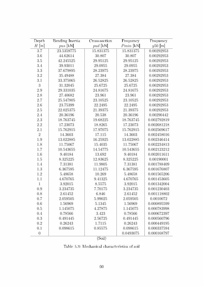
DepthH [m]
Bending Inertiapus [kN]
Cross-sectionpud [kN]
FrequencyPmin [kN]
Frequencyy50 [m]
3.7 23.5359775 15.831375 15.831375 0.002929533.6 44.62614 30.807 30.807 0.002929533.5 42.245525 29.95125 29.95125 0.002929533.4 39.93011 29.0955 29.0955 0.002929533.3 37.679895 28.23975 28.23975 0.002929533.2 35.49488 27.384 27.384 0.002929533.1 33.375065 26.52825 26.52825 0.002929533 31.32045 25.6725 25.6725 0.00292953
2.9 29.331035 24.81675 24.81675 0.002929532.8 27.40682 23.961 23.961 0.002929532.7 25.547805 23.10525 23.10525 0.002929532.6 23.75399 22.2495 22.2495 0.002929532.5 22.025375 21.39375 21.39375 0.002929532.4 20.36196 20.538 20.36196 0.002904422.3 18.763745 19.68225 18.763745 0.0027928192.2 17.23073 18.8265 17.23073 0.0026812182.1 15.762915 17.97075 15.762915 0.0025696172 14.3603 17.115 14.3603 0.002458016
1.9 13.022885 16.25925 13.022885 0.0023464141.8 11.75067 15.4035 11.75067 0.0022348131.7 10.543655 14.54775 10.543655 0.0021232121.6 9.40184 13.692 9.40184 0.0020116111.5 8.325225 12.83625 8.325225 0.001900011.4 7.31381 11.9805 7.31381 0.0017884091.3 6.367595 11.12475 6.367595 0.0016768071.2 5.48658 10.269 5.48658 0.0015652061.1 4.670765 9.41325 4.670765 0.0014536051 3.92015 8.5575 3.92015 0.001342004
0.9 3.234735 7.70175 3.234735 0.0012304030.8 2.61452 6.846 2.61452 0.0011188020.7 2.059505 5.99025 2.059505 0.00100720.6 1.56969 5.1345 1.56969 0.0008955990.5 1.145075 4.27875 1.145075 0.0007839980.4 0.78566 3.423 0.78566 0.0006723970.3 0.491445 2.56725 0.491445 0.0005607960.2 0.26243 1.7115 0.26243 0.0004491950.1 0.098615 0.85575 0.098615 0.0003375940 0.0493075 0.000168797
(Soil)
Table 5.3: Mechanical characteristics of soil
60

0 0.02 0.04 0.06 0.08 0.1 0.120
10
20
30
40
50
60
Displacement (m)
Load
(kN
)
Skeleton curve second specimen
Cd=0.12Cd=0.125Cd=0.13Cd=0.14SP2 data
Figure 5.7: Cd parameter calibration
61

62
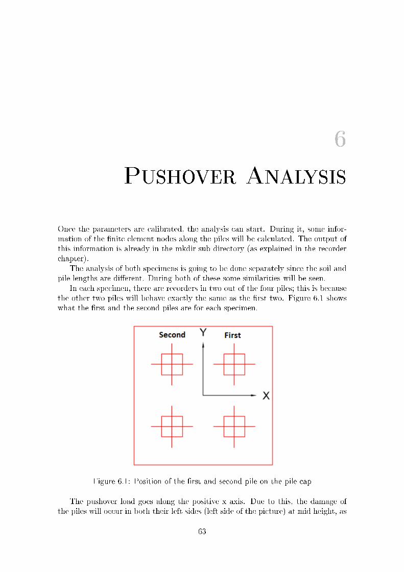
6
Pushover Analysis
Once the parameters are calibrated, the analysis can start. During it, some infor-mation of the �nite element nodes along the piles will be calculated. The output ofthis information is already in the mkdir sub directory (as explained in the recorderchapter).
The analysis of both specimens is going to be done separately since the soil andpile lengths are di�erent. During both of these some similarities will be seen.
In each specimen, there are recorders in two out of the four piles; this is becausethe other two piles will behave exactly the same as the �rst two. Figure 6.1 showswhat the �rst and the second piles are for each specimen.
Figure 6.1: Position of the �rst and second pile on the pile cap
The pushover load goes along the positive x axis. Due to this, the damage ofthe piles will occur in both their left sides (left side of the picture) at mid height, as
63

well as at the top right side of the pile.
6.1 First Specimen
The analysis will consist of a series of plots which will try to show the actual behaviorof the pile along the pushover load. Firstly, the position of some controlling timesteps are going to be de�ned. These time steps will de�ne the important momentsof the analysis and how the structure behavior is along them.
Here the position of these time steps are shown. Each one has a number so itcan be controlled later in the graphs 6.2
0 0.02 0.04 0.06 0.08 0.1 0.120
5
10
15
20
25
30
35
40
45
50
Displacement (m)
Load
(kN
)
Position of the Analysis Points
Skeleton1234567891011
Figure 6.2: Position of the analysis time steps
These time steps were chosen so the behavior of the structure during all thephases can be controlled. In the �rst time steps the structure behaves in an elasticway. Then, at around the 5 and 6 time steps, the �rst yielding occurs. This yieldingis the reason these time steps are so close, to control exactly when this occurs. Thenthe time steps are equidistant until the maximum load, which will be plotted too.Finally, the last point is the �nal failure of the structure. It will say when and howthe structure ultimately fails.
Figure 6.3 shows the evolution of the curvature along the height of the pile. Itis exactly the maximum curvature reached during the analysis.
As can be seen, the maximum curvature is reached just below the ground level(at 1 m deep). This result �ts the laboratory test data, as the biggest cracks anddamage of the experimental model occurred at the same height of the piles in thedata.
Due to the scale factor and the di�erence in magnitude of the failure pointcurvature and the rest of the curvatures, �gure 6.4 was done.
Figure 6.4 shows the time steps from 1 to 8. All of them are either behavingelastic or after the �rst yield, before the maximum load was reached. On thesecurves it can be seen that the �rst failure is produced on the top of the structure(0.8 m above the ground level).
64
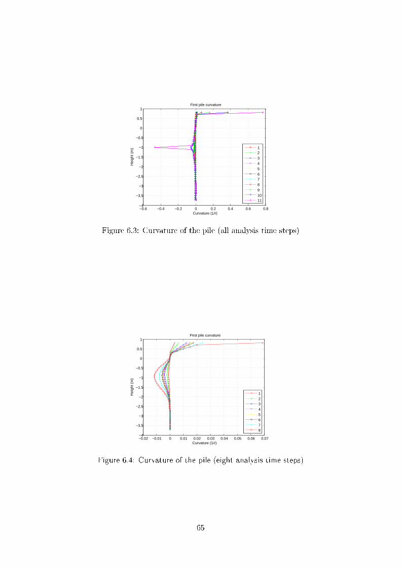
−0.6 −0.4 −0.2 0 0.2 0.4 0.6 0.8−4
−3.5
−3
−2.5
−2
−1.5
−1
−0.5
0
0.5
1
Curvature (1/r)
Hei
ght (
m)
First pile curvature
1234567891011
Figure 6.3: Curvature of the pile (all analysis time steps)
−0.02 −0.01 0 0.01 0.02 0.03 0.04 0.05 0.06 0.07−4
−3.5
−3
−2.5
−2
−1.5
−1
−0.5
0
0.5
1
Curvature (1/r)
Hei
ght (
m)
First pile curvature
12345678
Figure 6.4: Curvature of the pile (eight analysis time steps)
65

It is seen that the curvature increases in an elastic way until it reaches the seventhcurve, after that, it still increases but not elastically (meaning that the yielding hasalready happened at that section).
After this yield occurs at the top of the pile, at about −1 m under the groundlevel, the curvature increases with the opposite sign. This change in sign causes themodel to end up in the �gure that was shown before where the �nal failure pointhappens at that height.
The moment distribution will be similar to the curvature distribution, as it canbe seen in �gure 6.5.
−15 −10 −5 0 5 10−4
−3.5
−3
−2.5
−2
−1.5
−1
−0.5
0
0.5
1
Moment (kNm)
Hei
ght (
m)
First pile moment
1234567891011
Figure 6.5: Moment of the pile (all analysis time steps)
Here, the behavior is similar to the curvatures; �rst, the moment at the top ofthe piles (0.8 m) until it reaches the red line (number 9) where the section is alreadyyielded and the moment cannot be increased.
Then, with the increase of the load the next failure will be produced underthe ground level, at the same depth where the maximum curvature develops. Themaximum moment will be produced at the maximum pushover load and then thestructure will start to fail, having a lower moment carried out by the pile at itsultimate strength.
The next step is to calculate the distribution of the axial loads of the soil elementsalong the embedded height of the pile. This can be seen in the display 6.6.
The distribution of the time steps is di�erent than the other analysis becausetime steps were chosen so the behavior of the structure during all the phases canbe controlled. In the �rst time steps the structure behaves in an elastic way. Thenthe time steps are equidistant until the maximum load, which will be plotted too.Finally, the last point is the �nal failure of the structure. It will say when and howthe structure fails.
The axial load for the soil along the height of the pile is according to the analysistime steps already chosen in �gure 6.7.
As seen in the graph 6.7, the soil changes from being under compression on oneside of the pile, to being under compression on the other side. As it was seen inthe curvature plots, the change in the slope of the curve that is produced betweenthe depths of 1 and 2 m, ends up with this change in the sign of the axial load.
66

0 0.02 0.04 0.06 0.08 0.1 0.120
5
10
15
20
25
30
35
40
45
50
Displacement (m)
Load
(kN
)
Position of the Analysis Points
Skeleton12345678910
Figure 6.6: Position of the axail analysis time steps
−3.5 −3 −2.5 −2 −1.5 −1 −0.5 0 0.5 1 1.5−4
−3.5
−3
−2.5
−2
−1.5
−1
−0.5
0
Axil (kN)
Hei
ght (
m)
First pile soil axil
12345678910
Figure 6.7: Axial load pile-soil
67

With the increase of the pushover load, the axial load at the top of the ground willincrease until it reaches the maximum capacity of the sand. At the same time, theaxial load at the other side of the pile will increase too, but slower as it is not adirect relationship.
The soil will fail once it cannot withstand a larger load; the line number 10 showshow and where the soil fails. This failure is produced at a depth of −1 m, a littlebit below where the pile fails.
The �nal failure of this structure happens when the soil fails, after it, the pilewill increase its curvature failing too as it has not the soil to support it.
Now, the graph 6.8 shows the displacement of the nodes with the curvature.
−0.02 0 0.02 0.04 0.06 0.08 0.1 0.12 0.14 0.16−4
−3.5
−3
−2.5
−2
−1.5
−1
−0.5
0
0.5
1
Displacement (m)
Hei
ght (
m)
First pile node displacement
Node Displacement
Figure 6.8: Node max displacement
It can be seen that there is a little displacement in the negative side for a depthof −1.5 m approximately. This is the main cause of the change in the soil's axialload direction between a depth of 1 to 1.5 m.
6.2 Second Specimen
After �nishing with the analysis of the �rst specimen, the second can start. Theprocedure for this specimen will in fact be the same, although, the change in thepile length and the di�erent properties of the soil that already have been explainedwill end up giving a di�erent structure performance.
Again, the position of the controlling time steps are plotted (6.9); these timesteps have been picked so the exact point of the yielding of both sections results.
In this specimen, the yielding of the top section happens for a smaller load as itwill be seen later, so the time steps are closer to the beginning to predict the exactpoint of this yielding at this section.
Looking at �gure 6.10 the �nal failure is produced at a depth of 1.3 m, a depththat is higher than the �rst specimen, which means that the decrease of the pilelength over the ground makes the pile fail at a greater distance under the ground.Again, the scale factor is too sizable, so the distribution of curvatures at the top ofthe pile where the �rst yielding will occur cannot be seen. Due to this, another plot
68

0 0.02 0.04 0.06 0.08 0.1 0.120
10
20
30
40
50
60
Displacement (m)
Load
(kN
)
Position of the Analysis Points
Skeleton1234567891011
Figure 6.9: Position of the analysis time steps
is created that does not include the curves with a greater curvature, as is shown in�gure 6.11.
−0.6 −0.4 −0.2 0 0.2 0.4 0.6 0.8 1−4
−3.5
−3
−2.5
−2
−1.5
−1
−0.5
0
0.5
Curvature (1/r)
Hei
ght (
m)
First pile curvature
1234567891011
Figure 6.10: Curvature of the pile (all analysis time steps)
Here it can be seen that the curvature stops behaving in an elastic way at curvenumber eight, at the top of the pile. At this point the section has already yielded.
As in the other case, it is seen that at about −1.3 m under the ground level thecurvature increases with the opposite sign and it will end up failing at that depth,making the second plastic hinge.
Now, the moment distribution is plotted in �gure 6.12.For making this graph, the same time steps were used as for the curvature. The
results of �gure 6.12 indicate the same behavior as with the curvature. At the topof the structure (0.3 m) the moment cannot be increased after the yielding of thesection has already happened.
The �nal failure it is produced at about 1.3 m deep, and after that, the pile isnot able to withstand a moment as high as before (pink line with +).
For the soil analysis, the testing time steps that have been used are seen in �gure6.13.
69

−0.01 −0.005 0 0.005 0.01 0.015 0.02 0.025 0.03−4
−3.5
−3
−2.5
−2
−1.5
−1
−0.5
0
0.5
Curvature (1/r)
Hei
ght (
m)
First pile curvature
1234567
Figure 6.11: Curvature of the pile (eight analysis time steps)
−15 −10 −5 0 5 10−4
−3.5
−3
−2.5
−2
−1.5
−1
−0.5
0
0.5
Moment (kNm)
Hei
ght (
m)
First pile moment
1234567891011
Figure 6.12: Moment of the pile (all analysis time steps)
0 0.02 0.04 0.06 0.08 0.1 0.120
10
20
30
40
50
60
Displacement (m)
Load
(kN
)
Position of the Analysis Points
Skeleton12345678910
Figure 6.13: Position of the axial loads analysis times
70

They are more or less equally distributed because there is no need to calculatethe yielding of the top section, and it is enough with an approximation of how theaxial loads develop along the height. The only failure that will be seen is the �nalfailure and where it will be produced.
Using these time steps, the axial load for the soil along the height of the pile ofthe second specimen is (6.14).
−3 −2.5 −2 −1.5 −1 −0.5 0 0.5 1−4
−3.5
−3
−2.5
−2
−1.5
−1
−0.5
0
Axil (kN)
Hei
ght (
m)
First pile soil axil
12345678910
Figure 6.14: Axial load pile-soil
The soil has the same behavior as in the �rst specimen, although the failure isproduced at the depth of 1.3 m. The distribution of the load and why it changes itssign is similar as before.
The next plot will be the node displacement when the complete failure occurs.This plot will help to explain the reason of the distribution of the axial forces overthe soil.
From this curve, as before, it can be understood why the axial force changes itsdirection at a depth of about 1.5 to 2 m. The node displacement changes from beingpositive to negative at that point (6.15).
−0.02 0 0.02 0.04 0.06 0.08 0.1 0.12 0.14 0.16−4
−3.5
−3
−2.5
−2
−1.5
−1
−0.5
0
0.5
Displacement (m)
Hei
ght (
m)
First pile node displacement
Node Displacement
Figure 6.15: Node max displacement
71

72

7
Cyclic Analysis
This report has been written to model the deformation of a pile cap foundationuntil its failure. In this chapter the hysteresis loop will be used to complete deeperresearch in order to try to reproduce the laboratory test results. The hysteresis loopis the result of a cyclic load which will be controlled by several displacement steps.This means that there will be a �xed number of displacement steps to be reachedone by one. This cyclic analysis will attempt to represent what actually happenedin the experiment.
The hysteresis loop also represents the amount of energy that the structure candissipate before its failure. The bigger the area of this hysteresis loop, the greater theenergy that it can withstand. This is the reason why studying the cyclic analysis isso important for dynamics, because there is a direct relation between the structure'sdynamic performance and its energy dissipation. This relation is also called ductility.
The experiment, as it has previously been explained, was done under �xed cir-cumstances. The most important of these circumstances for this particular chapteris that the stresses of the di�erent structural members were not reset at the be-ginning of each cycle step (0 displacement), making both, the push (positive) andthe pull (negative) parts not symmetrical. This is because when plastic deformationoccurs, the structure will still present that deformation when no load is applied to it.It is also important to know that in the OpenSees model, the cyclic displacementswere programmed to be symmetrical.
The purpose of this model is to reproduce the real inelastic behavior of the pilecap under a cyclic displacement on the top of the piles using a simple �nite elementmodel.
While performing the computation of the OpenSees model some problems wereobserved, as it can be seen in �gure 7.1and 7.2. This is due to having calibratedthe model to the push part of the experimental data causing the curves of the pullpart of the loop to not �t as they should. My recommendation is that in a futureexperiment the model should be calibrated to both parts (pull and push) of thehysteresis curve (obtained in the laboratory) and not only to the push part.
73
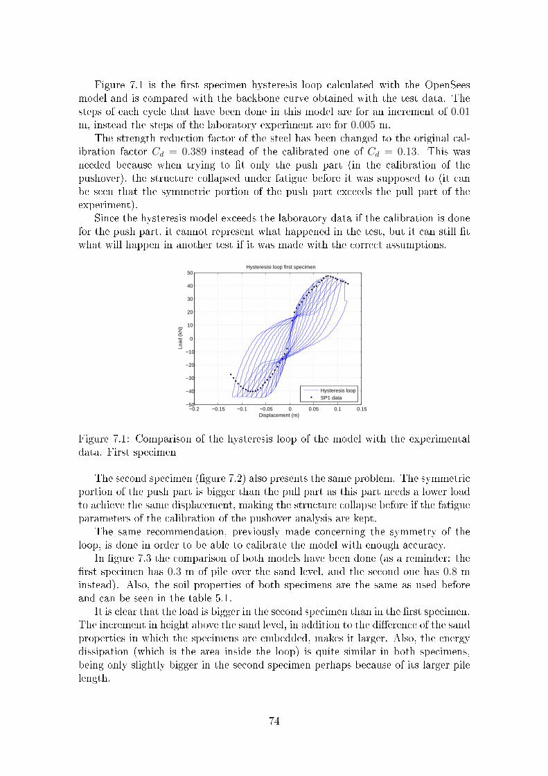
Figure 7.1 is the �rst specimen hysteresis loop calculated with the OpenSeesmodel and is compared with the backbone curve obtained with the test data. Thesteps of each cycle that have been done in this model are for an increment of 0.01m, instead the steps of the laboratory experiment are for 0.005 m.
The strength reduction factor of the steel has been changed to the original cal-ibration factor Cd = 0.389 instead of the calibrated one of Cd = 0.13. This wasneeded because when trying to �t only the push part (in the calibration of thepushover), the structure collapsed under fatigue before it was supposed to (it canbe seen that the symmetric portion of the push part exceeds the pull part of theexperiment).
Since the hysteresis model exceeds the laboratory data if the calibration is donefor the push part, it cannot represent what happened in the test, but it can still �twhat will happen in another test if it was made with the correct assumptions.
−0.2 −0.15 −0.1 −0.05 0 0.05 0.1 0.15−50
−40
−30
−20
−10
0
10
20
30
40
50
Displacement (m)
Load
(kN
)
Hysteresisi loop first specimen
Hysteresis loopSP1 data
Figure 7.1: Comparison of the hysteresis loop of the model with the experimentaldata. First specimen
The second specimen (�gure 7.2) also presents the same problem. The symmetricportion of the push part is bigger than the pull part as this part needs a lower loadto achieve the same displacement, making the structure collapse before if the fatigueparameters of the calibration of the pushover analysis are kept.
The same recommendation, previously made concerning the symmetry of theloop, is done in order to be able to calibrate the model with enough accuracy.
In �gure 7.3 the comparison of both models have been done (as a reminder: the�rst specimen has 0.3 m of pile over the sand level, and the second one has 0.8 minstead). Also, the soil properties of both specimens are the same as used beforeand can be seen in the table 5.1.
It is clear that the load is bigger in the second specimen than in the �rst specimen.The increment in height above the sand level, in addition to the di�erence of the sandproperties in which the specimens are embedded, makes it larger. Also, the energydissipation (which is the area inside the loop) is quite similar in both specimens,being only slightly bigger in the second specimen perhaps because of its larger pilelength.
74

−0.2 −0.15 −0.1 −0.05 0 0.05 0.1 0.15−60
−40
−20
0
20
40
60
Displacement (m)
Load
(kN
)
Hysteresis loop second specimen
Hysteresis loopSP1 data
Figure 7.2: Comparison of the hysteresis loop of the model with the experimentaldata. Second specimen
−0.2 −0.15 −0.1 −0.05 0 0.05 0.1 0.15−60
−40
−20
0
20
40
60
Displacement (m)
Load
(kN
)
Comparision of both OpenSees models
First modelSecond model
Figure 7.3: Comparison of the hysteresis loops of �rst and the second model
75

76

8
Conclusions
The model was built using OpenSees; this software is an open code provided byBerkley University and it has several tools to study the soil-structure interaction�eld, which is an area that is currently a serious concern, and a huge issue underinvestigation.
The model consists on two di�erent pile caps both with the same section andwith the same number of piles (4), but with a di�erence on the height of the pileabove the ground level. Both have 3.7 m of pile embedded on the sand and one ofthem has 0.3 m while the other has 0.8 m of pile above this ground level.
The program used is OpenSees because it allows to make nonlinear static analyses(capacity analysis) which will represent the ground motion acceleration. Thosenonlinear static analysis reproduce the inelastic behavior of the structural members.Predicting how and where the structure is going to fail.
There were both a pushover (capacity) analysis and a cyclic analysis. The failureanalysis was done using the pushover analysis, �nding out that the piles actuallyfail mainly in two positions:
• At the top of the structure (when joining the pile cap)
• Under the ground level
The �rst yielding point will be produced at the top of the piles for both specimens,although the force will change for both cases. For the �rst specimen, the force neededto make the top section fail will be slightly lower than for the second specimen, thisis due to the di�erence in length of the pile over the ground level.
The second yielding point will change its depth depending on the specimen. Forboth of them it will happen below the ground level, but for the �rst specimen itwill happen at 1 m deep but for the second one at 1.3 m. In both cases it canbe seen that the �nal failure point changes depending on the pushover load that isbeing applied. This means that before the yielding of the top section of the pilesoccurs, the maximum curvature will happen at −1 m and −1.3 m (depending on
77
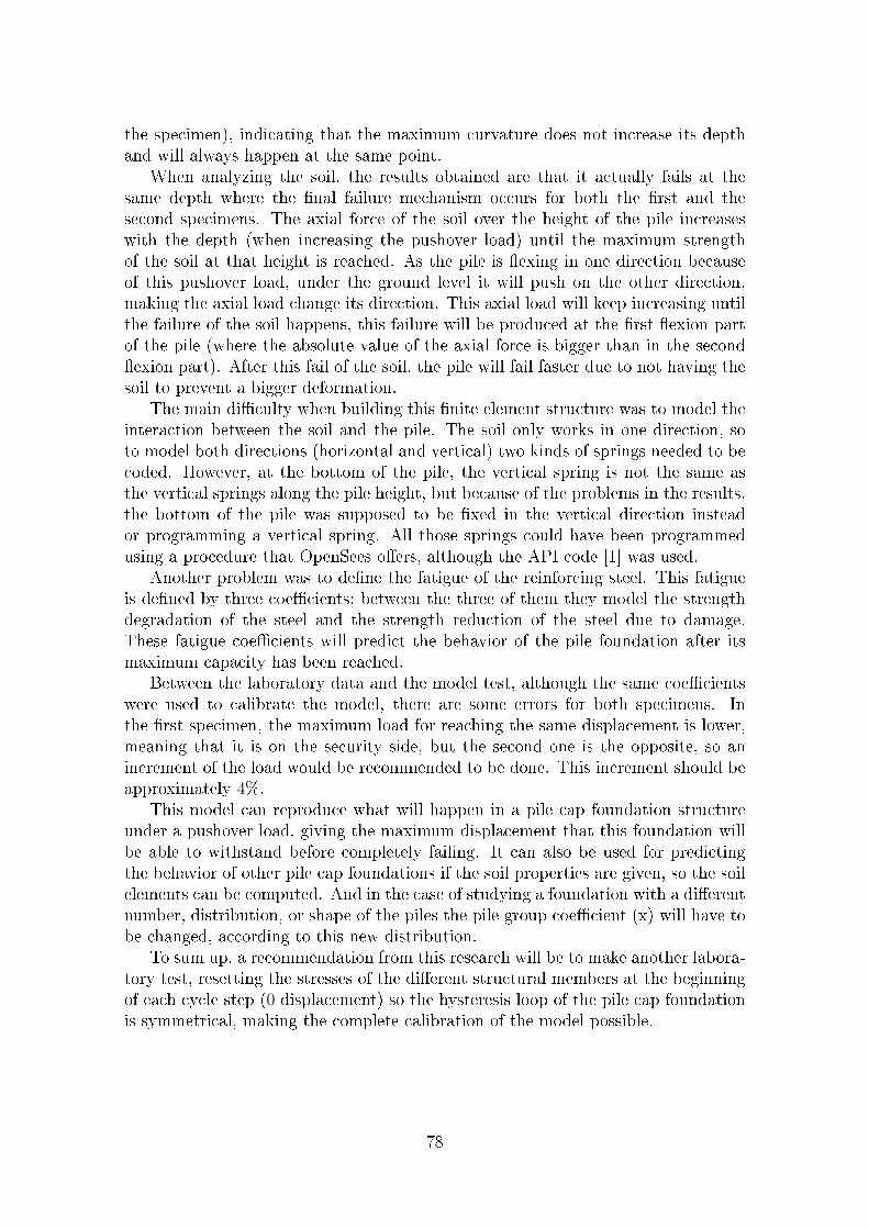
the specimen), indicating that the maximum curvature does not increase its depthand will always happen at the same point.
When analyzing the soil, the results obtained are that it actually fails at thesame depth where the �nal failure mechanism occurs for both the �rst and thesecond specimens. The axial force of the soil over the height of the pile increaseswith the depth (when increasing the pushover load) until the maximum strengthof the soil at that height is reached. As the pile is �exing in one direction becauseof this pushover load, under the ground level it will push on the other direction,making the axial load change its direction. This axial load will keep increasing untilthe failure of the soil happens, this failure will be produced at the �rst �exion partof the pile (where the absolute value of the axial force is bigger than in the second�exion part). After this fail of the soil, the pile will fail faster due to not having thesoil to prevent a bigger deformation.
The main di�culty when building this �nite element structure was to model theinteraction between the soil and the pile. The soil only works in one direction, soto model both directions (horizontal and vertical) two kinds of springs needed to becoded. However, at the bottom of the pile, the vertical spring is not the same asthe vertical springs along the pile height, but because of the problems in the results,the bottom of the pile was supposed to be �xed in the vertical direction insteador programming a vertical spring. All those springs could have been programmedusing a procedure that OpenSees o�ers, although the API code [1] was used.
Another problem was to de�ne the fatigue of the reinforcing steel. This fatigueis de�ned by three coe�cients; between the three of them they model the strengthdegradation of the steel and the strength reduction of the steel due to damage.These fatigue coe�cients will predict the behavior of the pile foundation after itsmaximum capacity has been reached.
Between the laboratory data and the model test, although the same coe�cientswere used to calibrate the model, there are some errors for both specimens. Inthe �rst specimen, the maximum load for reaching the same displacement is lower,meaning that it is on the security side, but the second one is the opposite, so anincrement of the load would be recommended to be done. This increment should beapproximately 4%.
This model can reproduce what will happen in a pile cap foundation structureunder a pushover load, giving the maximum displacement that this foundation willbe able to withstand before completely failing. It can also be used for predictingthe behavior of other pile cap foundations if the soil properties are given, so the soilelements can be computed. And in the case of studying a foundation with a di�erentnumber, distribution, or shape of the piles the pile group coe�cient (x) will have tobe changed, according to this new distribution.
To sum up, a recommendation from this research will be to make another labora-tory test, resetting the stresses of the di�erent structural members at the beginningof each cycle step (0 displacement) so the hysteresis loop of the pile cap foundationis symmetrical, making the complete calibration of the model possible.
78

Bibliography
[1] American Petroleum Institute, Recommended Practice for Planning, Designing,and Constructing Fixed O�shore Platforms Working Stress Design 21th Ed.,API RP2A-WSD, American Petroleum Institute, Washington, D.C., 2005
[2] Behrouz Asgarian and Mohammad Lesani, Pile soil-structure interaction inpushover analysis of jacket o�shore platforms using �ber elements Journal ofConstructional Steel Research, Vol.65, 1, 209-218, 2009
[3] California Seismic Safety Commission, Seismic Evaluation and Retro�t of Con-crete Buildings Applied Technology Council, November 1996 2009
[4] Antonio Bobet and Rodrigo Salgado and Dimitrios Loukidis, Seismic Designof Deep Foundations Purdue University, United States, 2001
[5] R. Boulanger and C. Currasand and B. Kutter and D. Wilson and A. Abghari,Seismic Soil-Pile-Structure Interaction Experiments and Analyses Journal ofGeotechnical and Geoenvironmental Engineering, Vol.125, 9, 750-759 1999
[6] S. Brandenberg and R. Boulangerand and B Kutter and D. Chang, StaticPushover Analyses of Pile Groups in Lique�ed and Laterally Spreading Groundin Centrifuge Tests Journal of Geotechnical and Geoenvironmental Engineer-ing, Vol.133, 9, 1055-1066 2007
[7] D. A. Brown and L. C. Reese, Lateral Load Behavior of Pile Group in SandJournal of Geotechnical Engineering, ASCE, Vol.114, 11, 1261-1276 1988
[8] Brown, J. and Kunnath, S.K., Low Cycle Fatigue Behavior of Longitudinal Re-inforcement in Reinforced Concrete Bridge Columns NCEER Technical Report00-0007, 2000
[9] Alfredo Camara, Seismic Behavior of Cable-Stayed Bridges: Design, Analysisand Seismic Devices NCEER Technical Report 00-0007, 2000
[10] T. C. Hutchinson, Characterization and Evaluation of the Seismic Performanceof Pile-supported Bridge Structures University of California, 2001
79

[11] G. A. Chang and John B. Mander, Seismic Energy Based Fatigue DamageAnalysis of Bridge Columns: Part I, Evaluation of Seismic Capacity NationalCenter for Earthquake Engineering Research, 1994
[12] Anil K. Chopra and Rakesh K. Goel, A Modal Pushover Analysis Procedure toEstimate Seismic Demands for Buildings: Theory and Preliminary EvaluationPEER, 2001
[13] L. F. Co�n, Transactions of ASME, Vol.76, 1954
[14] Deming Zhang, Experimental study on seismic performance of elevated pile-capfoundation of bridges Tongji University, Shanghai, China, 2012
[15] Dhakal, R. and Maekawa, K., Modeling for Postyield Buckled of ReinforcementJ. Struct. Eng., 128(9), 1139-1147, 2002
[16] Dhakal, R. P. and Maekawa, K., Reinforcement Stability and Fracture of CoverConcrete in Reinforced Concrete Members J. Struct. Eng., 0733-9445, 2002
[17] Dhakal, R. P. and Maekawa, K., Path-dependent cyclic stress-strain relationshipof reinforcing bar including buckling Engineering Structures 24, 1383-1396, 2002
[18] Ahmed Elgamal and Jinchi Lu, A Framework for 3D Finite Element Analysisof Lateral Pile System Response ASCE, 78, 613-623, 2009
[19] Gomes, A., and Appleton, J., Nonlinear Cyclic Stress-Strain Relationship ofReinforcing Bars Including Buckling Eng. Struct., 19(10), 822-826, 1997
[20] Balram Gupta and Sashi K. Kunnath, Adaptive Spectra-Based Pushover Proce-dure for Seismic Evaluation of Structures Earthquake Spectra, Vol.26, 2, 367-392 2000
[21] Department of California Highway Patrol, 1989 Loma Prieta Earthquake Sum-mary Report State of California, Dept. of California Highway Patrol 1989
[22] Lymon C. Reese,William F., Single Piles and Pile Groups Under Lateral Load-ing CRC Press, 2011
[23] Mander and M. J. N. Priestley, Theoretical Stress-strain Model for Con�nedConcrete Journal of Structural Engineering, Vol.114, 8, 1805-1826, 1988
[24] S. S. Manson, NACA Technical Note 2933, National Advisory Committee forAeronautics, Washington, D.C., 1953
[25] S. S. Manson, Fatigue: A Complex Subject-Some Simple Approximations Na-tional Aeronautics and Space Administration, Washington D.C., United States1964
[26] H. Matlock and W B Ingram and A. E. Kelley and D Bogard, Field Tests ofthe Lateral-load Behavior of Pile groups in Soft Clay 12th O�shore TechnologyConference, Houston, United States, 1980
80

[27] S Mazzoni and F McKenna and M H Scott and G L Fenves, OpenSees CommandLanguage University of California, Berkeley, 2007
[28] S Mazzoni and F McKenna and M H Scott and G L Fenves, Open System forEarthquake Engineering Simulation Paci�c Earthquake Engineering ResearchCenter, 1999
[29] Bramlette McClelland and J. A. Jr. Focht, Soil Modulus for Laterally LoadedPiles Transactions of ASCE, Vol.123, 1049-1086 1958
[30] Y. Meimon and F Baguelin and J F Jezequel, Field Tests of the Lateral-loadBehavior of Pile Groups in Soft Clay Third International Conference on Nu-merical Methods on O�shore Piling, Inst. Francais du Petrole, Nantes, France1986
[31] Menegotto, M. and Pinto, P. E., Method of analysis of cyclically loaded RCplane frames including changes in geometry and non-elastic behavior of ele-ments under normal force and bending Preliminary Report, IABSE, No. 13,pp. 15-22, 1973
[32] Philip James Meymand, Shaking Table Scale Model Tests of Nonlinear Soil-pile-superstructure Interaction in Soft Clay University of California, Berkeley,1998
[33] G. Mylonakis and G. Gazetas, Seismic Soil-structure Interaction: Bene�cial orDetrimental Journal of Earthquake Engineering, Vol.4, 3, 277-301 2000
[34] Ernest Naesgaard, Lateral Load Tests to Examine Large-strain(seismic) Be-haviour of Piles Canadian Geotechnical Journal, Vol.29, 2m 245-252, 1992
[35] S T Song, Limit State Analysis and Performance Assessment of Fixed-headConcrete Piles under Lateral Loading University of California, 2001
[36] Li Yan and Peter M. Byrne, Lateral pile response to monotonie pile head loadingCanadian Geotechnical Journal, Vol.29, 6, 955-970, 1992
[37] Zhaohui Yang and Boris Jeremi¢, Numerical study of group e�ects for pilegroups in sands International Journal for Numerical and Analytical Methodsin Geomechanics, Vol.27, 15, 1255-1276, 2003
[38] Arash E. Zaghi and M. Saiid Saiidi and Amir Mirmiran, Shake Table Responseand Analysis of a Concrete-�lled FRP Tube Bridge Column Composite Struc-tures, Vol.94, 5, 1564-1574, 2012
81

82

A
Code of the Finite
Element Model
In this Appendix the code that has been developed for OpenSees is attached. Thecode needs to be opened in a text editor. I chose Everedit from a wide variety, butany text editor could have been used. As it has already been said. OpenSees usestcl language in which # means comment.
As the code of both specimens is similar only the one of the �rst specimen willbe shown.
wipe ;
# un i t s m, t on s , KN
model Bas i cBu i lde r −ndm 3 −ndf 6
# Begin node d e f i n i n g
set h 0 . 1 ; # element length
set by 0 .225 ; # Bay width in Y−directionset bx 0 .225 ; # Bay width in X−direction
# tag X Y Z# p i l e 1for { set i 1} { $ i <= 46} { incr i 1} {node $ i [ expr $bx ] [ expr $by ] [ expr (−38+$ i ) ∗$h ]}
83
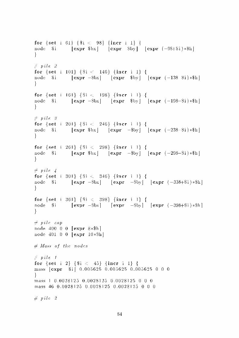
for { set i 61} { $ i <= 98} { incr i 1} {node $ i [ expr $bx ] [ expr $by ] [ expr (−98+$ i ) ∗$h ]}
# p i l e 2for { set i 101} { $ i <= 146} { incr i 1} {node $ i [ expr −$bx ] [ expr $by ] [ expr (−138+$ i ) ∗$h ]}
for { set i 161} { $ i <= 198} { incr i 1} {node $ i [ expr −$bx ] [ expr $by ] [ expr (−198+$ i ) ∗$h ]}
# p i l e 3for { set i 201} { $ i <= 246} { incr i 1} {node $ i [ expr $bx ] [ expr −$by ] [ expr (−238+$ i ) ∗$h ]}
for { set i 261} { $ i <= 298} { incr i 1} {node $ i [ expr $bx ] [ expr −$by ] [ expr (−298+$ i ) ∗$h ]}
# p i l e 4for { set i 301} { $ i <= 346} { incr i 1} {node $ i [ expr −$bx ] [ expr −$by ] [ expr (−338+$ i ) ∗$h ]}
for { set i 361} { $ i <= 398} { incr i 1} {node $ i [ expr −$bx ] [ expr −$by ] [ expr (−398+$ i ) ∗$h ]}
# p i l e capnode 400 0 0 [ expr 8∗$h ]node 401 0 0 [ expr 10∗$h ]
# Mass o f the nodes
# p i l e 1for { set i 2} { $ i <= 45} { incr i 1} {mass [ expr $ i ] 0 .005625 0 .005625 0 .005625 0 0 0}mass 1 0 .0028125 0 .0028125 0 .0028125 0 0 0mass 46 0 .0028125 0 .0028125 0 .0028125 0 0 0
# p i l e 2
84

for { set i 102} { $ i <= 145} { incr i 1} {mass [ expr $ i ] 0 .005625 0 .005625 0 .005625 0 0 0}mass 101 0 .0028125 0 .0028125 0 .0028125 0 0 0mass 146 0 .0028125 0 .0028125 0 .0028125 0 0 0
# p i l e 3for { set i 202} { $ i <= 245} { incr i 1} {mass [ expr $ i ] 0 .005625 0 .005625 0 .005625 0 0 0}mass 101 0 .0028125 0 .0028125 0 .0028125 0 0 0mass 146 0 .0028125 0 .0028125 0 .0028125 0 0 0
# p i l e 4for { set i 302} { $ i <= 345} { incr i 1} {mass [ expr $ i ] 0 .005625 0 .005625 0 .005625 0 0 0}mass 101 0 .0028125 0 .0028125 0 .0028125 0 0 0mass 146 0 .0028125 0 .0028125 0 .0028125 0 0 0
# p i l e capmass 401 1 1 1 0 0 0
# Set s o i l c on s t r a i n t s
# tag DX DY DZ RX RY RZ# p i l e 1for { set i 61} { $ i <= 98} { incr i 1} {f i x [ expr $ i ] 1 1 1 1 1 1}
#p i l e 2for { set i 161} { $ i <= 198} { incr i 1} {f i x [ expr $ i ] 1 1 1 1 1 1}
#p i l e 3for { set i 261} { $ i <= 298} { incr i 1} {f i x [ expr $ i ] 1 1 1 1 1 1}
#p i l e 4for { set i 361} { $ i <= 398} { incr i 1} {f i x [ expr $ i ] 1 1 1 1 1 1}
85

f i x 1 0 0 1 0 0 0f i x 101 0 0 1 0 0 0f i x 201 0 0 1 0 0 0f i x 301 0 0 1 0 0 0
# Define ma t e r i a l s f o r non l inear p i l e s
# Core concre te ( con f ined )
# tag f ' c epsc0 f ' cu epscuun i ax i a lMa t e r i a l Concrete01 1 −41850 −0.0024 −16740 −0.024
# Cover concre te ( unconf ined )
un i ax i a lMa t e r i a l Concrete01 2 −34250 −0.002 −13700 −0.006
# Rein forc ing s t e e l
# tag f y fu Es Esh esh eu −CMFatigue Cf a lpha Cdun i ax i a lMa t e r i a l Re i n f o r c i n gS t e e l 3 310000 459000 1 .54e81 .54e6 0 .024 0 .15 −CMFatigue 0 .26 0 .506 0 .13
set x 0 .55set y 3
# PyMateria ls
# tag f y fu Es Esh esh euun i ax i a lMa t e r i a l PySimple1 11 2 [ expr $x∗ 24 .57262500 ][ expr $y∗ 0 .001705148 ] 0 . 1 0un i ax i a lMa t e r i a l PySimple1 12 2 [ expr $x∗ 47 .81700000 ][ expr $y∗ 0 .001705148 ] 0 . 1 0un i ax i a lMa t e r i a l PySimple1 13 2 [ expr $x∗ 46 .48875000 ][ expr $y∗ 0 .001705148 ] 0 . 1 0un i ax i a lMa t e r i a l PySimple1 14 2 [ expr $x∗ 45 .16050000 ][ expr $y∗ 0 .001705148 ] 0 . 1 0un i ax i a lMa t e r i a l PySimple1 15 2 [ expr $x∗ 43 .83225000 ][ expr $y∗ 0 .001705148 ] 0 . 1 0un i ax i a lMa t e r i a l PySimple1 16 2 [ expr $x∗ 42 .50400000 ][ expr $y∗ 0 .001705148 ] 0 . 1 0un i ax i a lMa t e r i a l PySimple1 17 2 [ expr $x∗ 41 .17575000 ][ expr $y∗ 0 .001705148 ] 0 . 1 0un i ax i a lMa t e r i a l PySimple1 18 2 [ expr $x∗ 39 .84750000 ][ expr $y∗ 0 .001705148 ] 0 . 1 0un i ax i a lMa t e r i a l PySimple1 19 2 [ expr $x∗ 38 .51925000 ][ expr $y∗ 0 .001705148 ] 0 . 1 0
86

un i ax i a lMa t e r i a l PySimple1 20 2 [ expr $x∗ 37 .19100000 ][ expr $y∗ 0 .001705148 ] 0 . 1 0un i ax i a lMa t e r i a l PySimple1 21 2 [ expr $x∗ 35 .86275000 ][ expr $y∗ 0 .001705148 ] 0 . 1 0un i ax i a lMa t e r i a l PySimple1 22 2 [ expr $x∗ 34 .53450000 ][ expr $y∗ 0 .001705148 ] 0 . 1 0un i ax i a lMa t e r i a l PySimple1 23 2 [ expr $x∗ 33 .20625000 ][ expr $y∗ 0 .001705148 ] 0 . 1 0un i ax i a lMa t e r i a l PySimple1 24 2 [ expr $x∗ 30 .77676000 ][ expr $y∗ 0 .001646243 ] 0 . 1 0un i ax i a lMa t e r i a l PySimple1 25 2 [ expr $x∗ 28 .34646500 ][ expr $y∗ 0 .001582171 ] 0 . 1 0un i ax i a lMa t e r i a l PySimple1 26 2 [ expr $x∗ 26 .01599000 ][ expr $y∗ 0 .001518099 ] 0 . 1 0un i ax i a lMa t e r i a l PySimple1 27 2 [ expr $x∗ 23 .78533500 ][ expr $y∗ 0 .001454027 ] 0 . 1 0un i ax i a lMa t e r i a l PySimple1 28 2 [ expr $x∗ 21 .65450000 ][ expr $y∗ 0 .001389954 ] 0 . 1 0un i ax i a lMa t e r i a l PySimple1 29 2 [ expr $x∗ 19 .62348500 ][ expr $y∗ 0 .001325882 ] 0 . 1 0un i ax i a lMa t e r i a l PySimple1 30 2 [ expr $x∗ 17 .69229000 ][ expr $y∗ 0 .00126181 ] 0 . 1 0un i ax i a lMa t e r i a l PySimple1 31 2 [ expr $x∗ 15 .86091500 ][ expr $y∗ 0 .001197738 ] 0 . 1 0un i ax i a lMa t e r i a l PySimple1 32 2 [ expr $x∗ 14 .12936000 ][ expr $y∗ 0 .001133665 ] 0 . 1 0un i ax i a lMa t e r i a l PySimple1 33 2 [ expr $x∗ 12 .49762500 ][ expr $y∗ 0 .001069593 ] 0 . 1 0un i ax i a lMa t e r i a l PySimple1 34 2 [ expr $x∗ 10 .96571000 ][ expr $y∗ 0 .001005521 ] 0 . 1 0un i ax i a lMa t e r i a l PySimple1 35 2 [ expr $x∗ 9 .53361500 ][ expr $y∗ 0 .000941449 ] 0 . 1 0un i ax i a lMa t e r i a l PySimple1 36 2 [ expr $x∗ 8 .20134000 ][ expr $y∗ 0 .000877376 ] 0 . 1 0un i ax i a lMa t e r i a l PySimple1 37 2 [ expr $x∗ 6 .96888500 ][ expr $y∗ 0 .000813304 ] 0 . 1 0un i ax i a lMa t e r i a l PySimple1 38 2 [ expr $x∗ 5 .83625000 ][ expr $y∗ 0 .000749232 ] 0 . 1 0un i ax i a lMa t e r i a l PySimple1 39 2 [ expr $x∗ 4 .80343500 ][ expr $y∗ 0 .00068516 ] 0 . 1 0un i ax i a lMa t e r i a l PySimple1 40 2 [ expr $x∗ 3 .87044000 ][ expr $y∗ 0 .000621087 ] 0 . 1 0un i ax i a lMa t e r i a l PySimple1 41 2 [ expr $x∗ 3 .03726500 ][ expr $y∗ 0 .000557015 ] 0 . 1 0un i ax i a lMa t e r i a l PySimple1 42 2 [ expr $x∗ 2 .30391000 ][ expr $y∗ 0 .000492943 ] 0 . 1 0
87

un i ax i a lMa t e r i a l PySimple1 43 2 [ expr $x∗ 1 .67037500 ][ expr $y∗ 0 .000428871 ] 0 . 1 0un i ax i a lMa t e r i a l PySimple1 44 2 [ expr $x∗ 1 .13666000 ][ expr $y∗ 0 .000364798 ] 0 . 1 0un i ax i a lMa t e r i a l PySimple1 45 2 [ expr $x∗ 0 .70276500 ][ expr $y∗ 0 .000300726 ] 0 . 1 0un i ax i a lMa t e r i a l PySimple1 46 2 [ expr $x∗ 0 .36869000 ][ expr $y∗ 0 .000236654 ] 0 . 1 0un i ax i a lMa t e r i a l PySimple1 47 2 [ expr $x∗ 0 .13443500 ][ expr $y∗ 0 .000172582 ] 0 . 1 0un i ax i a lMa t e r i a l PySimple1 48 2 [ expr $x∗ 0 .06721750 ][ expr $y∗ 8 .62908E−05 ] 0 . 1 0
# Column se c t i on# s e t some paramatersset colWidth 0 .15set colDepth 0 .15
set cover 0 . 02set As 0 .0001131
# some v a r i a b l e s de r i v ed from the parametersset y1 [ expr $colDepth /2 . 0 ]set z1 [ expr $colWidth /2 . 0 ]
# sec t i on Fibers e c t i o n Fiber 100 {
# Create the concre te core f i b e r spatch quad 1 5 5 [ expr $cover−$y1 ] [ expr $cover−$z1 ] [ expr$y1−$cover ] [ expr $cover−$z1 ] [ expr $y1−$cover ] [ expr$z1−$cover ] [ expr $cover−$y1 ] [ expr $z1−$cover ]
# Create the concre te cover f i b e r spatch quad 2 10 2 [ expr −$y1 ] [ expr $z1−$cover ] $y1 [ expr$z1−$cover ] $y1 $z1 [ expr −$y1 ] $z1patch quad 2 10 2 [ expr −$y1 ] [ expr −$z1 ] $y1 [ expr −$z1 ]$y1 [ expr $cover−$z1 ] [ expr −$y1 ] [ expr $cover−$z1 ]patch quad 2 2 10 [ expr −$y1 ] [ expr $cover−$z1 ] [ expr$cover−$y1 ] [ expr $cover−$z1 ] [ expr $cover−$y1 ] [ expr$z1−$cover ] [ expr −$y1 ] [ expr $z1−$cover ]patch quad 2 2 10 [ expr $y1−$cover ] [ expr $cover−$z1 ] $y1[ expr $cover−$z1 ] $y1 [ expr $z1−$cover ] [ expr $y1−$cover ][ expr $z1−$cover ]
# Create the r e i n f o r c i n g f i b e r s
88

# $matTag $numBars $areaBar $yS tar t $ zS t a r t $yEnd $zEndl a y e r s t r a i g h t 3 2 $As [ expr −$y1+$cover ] [ expr −$z1+$cover ][ expr −$y1+$cover ] [ expr $z1−$cover ]l a y e r s t r a i g h t 3 2 $As [ expr −$y1+$cover ] [ expr −$z1+$cover ][ expr $y1−$cover ] [ expr −$z1+$cover ]}
un i ax i a lMa t e r i a l E l a s t i c 101 1e10
set PileSecTag 1 ;s e c t i o n Aggregator $PileSecTag 101 T −sect ion 100
# Define p i l e e lements
geomTransf Linear 10 1 0 0
# Number o f column i n t e g r a t i o n po in t s ( s e c t i o n s )set np 3# Create the non l inear p i l e e lements# tag ndI ndJ nPts secID t r an s f# p i l e 1for { set j 1} { $ j <= 45} { incr j 1} {element dispBeamColumn [ expr $ j ] [ expr $ j ] [ expr $ j +1]$np 1 10}
# p i l e 2for { set j 101} { $ j <= 145} { incr j 1} {element dispBeamColumn [ expr $ j ] [ expr $ j ] [ expr $ j +1]$np 1 10}
# p i l e 3for { set j 201} { $ j <= 245} { incr j 1} {element dispBeamColumn [ expr $ j ] [ expr $ j ] [ expr $ j +1]$np 1 10}
# p i l e 4for { set j 301} { $ j <= 345} { incr j 1} {element dispBeamColumn [ expr $ j ] [ expr $ j ] [ expr $ j +1]$np 1 10}
# Define p i l e cap e lements
89

# Geometric t rans format ion f o r p i l e cap e lements# tag vecxzgeomTransf Linear 20 0 0 1
# tag ndI ndJ A E G J Iy I z t r an s felement elasticBeamColumn 401 46 400 1e2 2e8 1e8 0 . 2 0 . 20 . 2 20element elasticBeamColumn 402 146 400 1e2 2e8 1e8 0 . 2 0 . 20 . 2 20element elasticBeamColumn 403 246 400 1e2 2e8 1e8 0 . 2 0 . 20 . 2 20element elasticBeamColumn 404 346 400 1e2 2e8 1e8 0 . 2 0 . 20 . 2 20element elasticBeamColumn 405 400 401 1e2 2e8 1e8 0 . 2 0 . 20 . 2 10
source TzMat e r i a l s 1 . t c l# Done through the TzMaterial1Gen command
# Create the s o i l e lements
# eleTag iNode jNode mat# p i l e 1for { set j 62} { $ j <= 98} { incr j 1} {element zeroLength $ j [ expr $j−60 ] $ j −mat [ expr $j−50 ][ expr $j−2 ] −dir 1 3}element zeroLength 61 1 61 −mat 11 −dir 1
# p i l e 2for { set j 162} { $ j <= 198} { incr j 1} {element zeroLength $ j [ expr $j−60 ] $ j −mat [ expr $j−150 ][ expr $j−102 ] −dir 1 3}element zeroLength 161 101 161 −mat 11 −dir 1
# p i l e 3for { set j 262} { $ j <= 298} { incr j 1} {element zeroLength $ j [ expr $j−60 ] $ j −mat [ expr $j−250 ][ expr $j−202 ] −dir 1 3}element zeroLength 261 201 261 −mat 11 −dir 1
# p i l e 4
90

for { set j 362} { $ j <= 398} { incr j 1} {element zeroLength $ j [ expr $j−60 ] $ j −mat [ expr $j−350 ][ expr $j−302 ] −dir 1 3}element zeroLength 361 301 361 −mat 11 −dir 1
# Define g r a v i t y l oads
# Create a Plain load pa t t e rn wi th a Linear TimeSeries
pattern Pla in 1 "Linear " {# nd FX FY FZ MX MY MZ# p i l e 1for { set k 2} {$k <= 45} { incr k 1} {load $k 0 0 −0.055125 0 0 0}load 1 0 0 −0.0275625 0 0 0load 46 0 0 −0.0275625 0 0 0
# p i l e 2for { set k 102} {$k <= 145} { incr k 1} {load $k 0 0 −0.055125 0 0 0}load 101 0 0 −0.0275625 0 0 0load 146 0 0 −0.0275625 0 0 0
# p i l e 3for { set k 202} {$k <= 245} { incr k 1} {load $k 0 0 −0.055125 0 0 0}load 201 0 0 −0.0275625 0 0 0load 246 0 0 −0.0275625 0 0 0
# p i l e 4for { set k 302} {$k <= 345} { incr k 1} {load $k 0 0 −0.055125 0 0 0}load 301 0 0 −0.0275625 0 0 0load 346 0 0 −0.0275625 0 0 0
# p i l e capload 401 0 0 −9.81 0 0 0}
# Gravi ty ana l y s i s
91

system BandGeneralc on s t r a i n t s Transformationnumberer RCMt e s t NormDispIncr 1 .0e−12 10 3a lgor i thm Newtoni n t e g r a t o r LoadControl 0 . 1an a l y s i s S t a t i ci n i t i a l i z eset ok [ ana lyze 10 ]loadConst −time 0 . 0
# Pushover or Cyc l i c ana l y s i s
set IDctrlNode 401 ;set IDctrlDOF 1 ;set iDmax "0 .12 " ; # i f pushover# se t iDmax "0 .005 0 .010 0 .015 0 .020 0 .025 0 .030 0 .040 0 .0500 .060 0 .070 0 .080 0 .090 0 .10 0 .11 0 .12 " ; # i f cy c l es e t Dincr 0 .001 ;s e t Fact 1 ;s e t Ncyc les 1 ;
# AnalysisType s e l e c t i o n
# Chose between Cycle or Pushover
# s e t AnalysisType Ful lCyc le ;s e t AnalysisType Pushover ;
# Create load pattern f o r l a t e r a l load ana l y s i s
s e t Hload 1 ;pattern Pla in 200 Linear { ;load $IDctrlNode $Hload 0 . 0 0 . 0 0 . 0 0 . 0 0 . 0 ;}
i f { $AnalysisType == "Ful lCyc le "} {puts " Star t Ful lCyc le "}i f { $AnalysisType == "Pushover"} {puts " Star t Pushover Ana lys i s "}
# Set up ana l y s i s parameters
source S t a t i cAna l y s i sCon t r o l l i n gPa r ame t e r s . t c l ;
92

# Perform the Ana lys i s
proc GeneratePeaks {Dmax {Dinc rS ta t i c 0 .001 } {AnalysisType"Ful lCyc le "} {Fact 1} } { ;# generate incrementa l d i sp s f o r Dmaxf i l e mkdir datas e t outFi le ID [ open data/ tmpDsteps . tc l w]s e t Disp 0 . 0puts $outFi le ID " set iDstep { " ;# open vec to r d e f i n i t i o ns e t Dmax [ expr $Dmax∗$Fact ] ;# s c a l e valuei f {$Dmax<0} { ;# avoid the d iv id e by zeros e t dx [ expr −$DincrStat ic ]} e l s e {s e t dx $Dinc rSta t i c ;}s e t NstepsPeak [ expr i n t ( abs ($Dmax)/ $Dinc rSta t i c ) ]f o r { s e t i 1} { $ i <= $NstepsPeak} { i n c r i 1} { ;# zero to one Dmaxs e t Disp [ expr $Disp + $dx ]puts $outFi le ID $Disp ;# wr i t e to f i l e}i f { $AnalysisType !="Pushover"} {f o r { s e t i 1} { $ i <= $NstepsPeak} { i n c r i 1} { ;# one Dmax to zeros e t Disp [ expr $Disp − $dx ]puts $outFi le ID $Disp ;# wr i t e to f i l e}}puts $outFi le ID " }" ;# c l o s e vec to r d e f i n i t i o nc l o s e $outFi le IDsource data/ tmpDsteps . tc l ;# source t c l f i l e to d e f i n e e n t i r e vec to rre turn $iDstep}
fo r each Dmax $iDmax {s e t iDstep [ GeneratePeaks $Dmax $Dincr $AnalysisType $Fact ] ;f o r { s e t i 1} { $ i <= $Ncycles } { i n c r i 1} {puts "push to $Dmax m" ;
93

s e t D0 0 . 0f o r each Dstep $iDstep {s e t D1 $Dsteps e t Dincr [ expr $D1 − $D0 ]i n t e g r a t o r DisplacementControl $IDctrlNode $IDctrlDOF $Dincran a l y s i s S t a t i c# F i r s t ana lyze commands e t ok [ ana lyze 1 ]# I f convergence f a i l si f {$ok != 0} {# i f an a l y s i s f a i l s , t r i e s other a lgor i thmsi f {$ok != 0} {puts "Trying Newton with I n i t i a l Tangent . . . "t e s t NormDispIncr $To lS ta t i c 2000 0s e t ok [ ana lyze 1 ]t e s t $ te s tTypeStat i c $To lS ta t i c $maxNumIterStatic 0}i f {$ok != 0} {puts "Trying Broyden . . . "a lgor i thm Broyden 8s e t ok [ ana lyze 1 ]a lgor i thm $algor i thmTypeStat ic}i f {$ok != 0} {puts "Trying NewtonWithLineSearch . . "a lgor i thm NewtonLineSearch 0 . 8s e t ok [ ana lyze 1 ]a lgor i thm $algor i thmTypeStat ic}i f {$ok != 0} {s e t putout [ format "Ana lys i s t e rmina l d i sp "[ nodeDisp $IDctrlNode $IDctrlDOF ] ]puts $putoutre turn −1} ;} ; # end i fs e t D0 $D1 ; # move to next step} ; # end inner fo r each} ; # end f o r} ; # end outer f o r each
i f {$ok != 0 } {puts [ format "Ana lys i s t e rmina l d i s p : " "PROBLEM"[ nodeDisp $IDctrlNode $IDctrlDOF ] ]} e l s e {puts [ format "Ana lys i s t e rmina l d i s p : " "DONE"
94

[ nodeDisp $IDctrlNode $IDctrlDOF ] ]}
i f {$ok != 0 && $AnalysisType == "Pushover"} {puts "Pushover Ana lys i s Fa i l ed "} e l s e i f { $AnalysisType == "Pushover"} {puts "Pushover Ana lys i s Succeeded"}
i f {$ok != 0 && $AnalysisType == "Ful lCyc le "} {puts " Ful lCyc le Ana lys i s Fa i l ed "} e l s e i f { $AnalysisType == "Ful lCyc le "} {puts " Ful lCyc le Ana lys i s Succeeded"}
95

96


![Pile Foundation Design[1] - ITDmtp.itd.co.th/ITD-CP/data/PileFoundationDesign.pdf · Introduction to pile foundations Pile foundation design Load on piles Single pile design Pile](https://img.pdfslide.net/doc/110x75/5a6ffb387f8b9ab1538b8376/pile-foundation-design1-itdmtpitdcothitd-cpdatapilefoundationdesignpdfpdf.jpg)