Seismic Solar Models from Ledoux discriminant inversions

arX

iv:2

007.

1022

2v1

[as

tro-

ph.S

R]

20

Jul 2

020

Astronomy & Astrophysics manuscript no. PaperSismo c©ESO 2020July 21, 2020

Seismic Solar Models from Ledoux discriminant inversions

G. Buldgen1, P. Eggenberger1 , V.A. Baturin2, T. Corbard3, J.Christensen-Dalsgaard4 , S. J. A. J. Salmon1, 5, A. Noels5,

A. V. Oreshina2, and R. Scuflaire5

1 Observatoire de Genève, Université de Genève, 51 Ch. Des Maillettes, CH−1290 Sauverny, Suisse2 Sternberg Astronomical Institute, Lomonosov Moscow State University, 119234 Moscow, Russia3 Université Côte d’Azur, Observatoire de la Côte d’Azur, CNRS, Laboratoire Lagrange, France4 Stellar Astrophysics Centre and Department of Physics and Astronomy, Aarhus University, DK-8000 Aarhus C, Denmark5 STAR Institute, Université de Liège, Allée du Six Août 19C, B−4000 Liège, Belgium

January, 2020

ABSTRACT

Context. The Sun constitutes an excellent laboratory of fundamental physics. With the advent of helioseismology, we were able toprobe its internal layers with unprecendented precision and thoroughness. However, the current state of solar modelling is still stainedby tedious issues. One of these central problems is related to the disagreement between models computed with recent photosphericabundances and helioseismic constraints. The observed discrepancies raise questions on some fundamental ingredients entering thecomputation of solar and stellar evolution models.Aims. We use solar evolutionary models as initial conditions for reintegrations of their structure using Ledoux discriminant inversions.The resulting models are defined as seismic solar models, satisfying the equations of hydrostatic equilibrium. These seismic modelswill allow us to better constrain the internal structure of the Sun and provide complementary information to that of calibrated standardand non-standard models.Methods. We use inversions of the Ledoux discriminant to reintegrate seismic solar models satisfying the equations of hydrostaticequilibrium. These seismic models were computed using various reference models with different equations of state, abundances andopacity tables. We check the robustness of our approach by confirming the good agreement of our seismic models in terms of soundspeed, density and entropy proxy inversions as well as frequency-separation ratios of low-degree pressure modes.Results. Our method allows us to determine with an excellent accuracy the Ledoux discriminant profile of the Sun and compute fullprofiles of this quantity. Our seismic models show an agreement with seismic data of ≈ 0.1% in sound speed, density and entropyproxy after 7 iterations in addition to an excellent agreement with the observed frequency-separation ratios. They surpass all standardand non-standard evolutionary models including ad-hoc modifications of their physical ingredients aiming at reproducing helioseismicconstraints.Conclusions. The obtained seismic Ledoux discriminant profile as well as the full consistent structure obtained from our reconstruc-tion procedure paves the way for renewed attempts at constraining the solar modelling problem and the missing physical processesacting in the solar interior by breaking free from the hypotheses of evolutionary models.

Key words. Sun: helioseismology – Sun: oscillations – Sun: fundamental parameters – Sun: interior

1. Introduction

Over the course of the 20th century, the field of helio-seismology has encountered major successes and has pro-vided us highly precise measurements of the internal prop-erties of the Sun. Thanks to the exquisite observationaldata taken over decades, seismology of the Sun has al-lowed to determine precisely the position of the base ofthe solar convective zone (Christensen-Dalsgaard et al. 1991;Kosovichev & Fedorova 1991; Basu & Antia 1997), to mea-sure the current helium abundance in the convective zone(Vorontsov et al. 1991; Dziembowski et al. 1991; Antia & Basu1994a; Basu & Antia 1995; Richard et al. 1998) as well as the2D profile of the rotational velocity (Brown & Morrow 1987;Thompson et al. 1996; Howe 2009) and the radial profile ofstructural quantities inside the Sun such as sound speed anddensity (e.g. Christensen-Dalsgaard et al. 1985; Antia & Basu1994b; Marchenkov et al. 2000, for some illustrations includ-ing non-linear techniques and the first direct inversion of sound-speed from the asymptotic expression of pressure modes). These

results of unprecedented quality are at the origin of key ques-tions for solar and stellar physics, showing the crucial role of theSun and stars as laboratories of fundamental physics.

Amongst them, the revision of the solar abundances starting al-most two decades ago and culminating in Asplund et al. (2009)caused a crisis in the solar modelling community that still awaitsa definitive solution (see e.g. Antia & Basu 2005; Guzik et al.2006; Montalban et al. 2006; Zaatri et al. 2007; Serenelli et al.2009; Guzik & Mussack 2010; Bergemann & Serenelli 2014;Zhang 2014, and references therein for additional discussions).The recent experimental measurement of opacity by Bailey et al.(2015) and Nagayama et al. (2019) confirmed the suspicions ofthe community that the source of the observed discrepancieswith revised abundances could stem from the theoretical opac-ity tables used for solar models. However, while these certainlyrepresent the main suspect, other contributors may well have anon-negligible impact in the total quantitative analysis of themismatch between seismic data and evolutionary models of theSun.

Article number, page 1 of 15

http://arxiv.org/abs/2007.10222v1

A&A proofs: manuscript no. PaperSismo

Recently, Buldgen et al. (2019) analysed in depth the dif-ferent contributors to the solar modelling problem us-ing a combination of inversion techniques. They alsoshowed that none of the current combinations of physi-cal ingredients could restore the agreement between low-metallicity standard evolutionary solar models and helio-seismic constraints to the level of high-metallicity stan-dard evolutionary solar models. Similarly to earlier studies(Basu & Antia 2008; Christensen-Dalsgaard & Houdek 2010;Ayukov & Baturin 2011, 2017; Christensen-Dalsgaard et al.2018), they concluded that a local increase in opacity was alsoinsufficient to restore the agreement of low-metallicity evolu-tionary models with helioseismic data. They also analysed indepth the interplay between different physical ingredients suchas the hypotheses made when computing microscopic diffusion,the equation of state and the formalism used for convectionand showed that they could lead to small but significant differ-ences at the level of precision expected from helioseismic infer-ences.

Consequently, further constraining the required changes tosolve the solar modelling problem might require to stepout of the framework of evolutionary models, trying toprovide direct seismic constraints on the possible inaccu-racies of microphysical ingredients as well as macroscopicprocesses not included in the current standard solar mod-els. To do so, a promising approach is to try to rebuildthe solar structure as seen from helioseismic data, as donein e.g. Shibahashi et al. (1995), Shibahashi & Takata (1996),Basu & Thompson (1996) , Gough & Scherrer (2001), Gough(2004) and Turck-Chièze et al. (2004), and use this static struc-ture to provide insights on potential revision of key ingredientsof solar and stellar models. In this paper, we present a new ap-proach to rebuild the solar structure based on inversions of theLedoux discriminant, defined as

A =1

Γ1

d ln P

d ln r− d ln ρ

d ln r. (1)

We demonstrate that the procedure converges on a unique so-lution for the Ledoux discriminant profile after only a few it-erations and that the final structure for this new “seismic Sun”also agrees very well with all other structural inversions suchas those of density, sound speed and entropy proxy defined inBuldgen et al. (2017d) as

S 5/3 =P

ρ5/3. (2)

A main advantage of the reconstruction procedure is that it pro-vides a full profile of the Ledoux discriminant without the needof numerical differentiation. However, this does not mean thatthe method is devoid of interpolations when constructing theseismic models.

The goal of our reconstruction procedure is to provide a clearerinsight as to the requirements of a revision of the opacity ta-bles in solar conditions, which are the subject of discussion inthe opacity community (see e.g. Iglesias 2015; Nahar & Pradhan2016; Blancard et al. 2016; Iglesias & Hansen 2017; Pain et al.2018; Pradhan & Nahar 2018; Zhao et al. 2018; Pain & Gilleron2019, 2020, and references therein) following the experimen-tal measurements of Bailey et al. (2015) and Nagayama et al.(2019). Consequently, we mainly focus on the reproduction ofthe profile of structural quantities in the radiative region of the

Sun, where uncertainties in the solar Γ1 profile may be con-sidered negligible in the A profile determined from the inver-sion.

In addition, it can be shown that the behaviour of the A profilein the deep radiative layers is mostly determined by the temper-ature gradient, the mean molecular weight gradient only con-tributing to the expression of A near the base of the convectivezone and in regions affected by nuclear reactions. Consequently,we can have a direct measurement of the temperature gradi-ent in these regions and directly quantify the required changesof opacity for various chemical compositions and underlyingequations of state, once the internal structure has been reliablydetermined. Such a determination is complementary to the ap-proaches used for example in Christensen-Dalsgaard & Houdek(2010), Ayukov & Baturin (2017) and Buldgen et al. (2019),where ad-hoc modifications were applied in calibrated solarmodels. These measurements are to be compared to the expectedrevisions of theoretical opacity computations and the current ex-perimental measurements available, helping guide a revision ofstandard ingredients of solar models by providing additional “ex-perimental” opacity estimations directly from helioseismic ob-servations 1.

Near the base of the solar convective zone, our ap-proach will provide a complementary method to that ofChristensen-Dalsgaard et al. (2018) in studying the hydro-static structure of the solar tachocline2 (Spiegel & Zahn1992). Indeed, the properties of the mean molecular weightgradients in this region play a key role in understand-ing the angular momentum transport mechanisms acting inthe solar interior (Gough & McIntyre 1998; Spruit 1999;Charbonnel & Talon 2005; Eggenberger et al. 2005; Spada et al.2010; Eggenberger et al. 2019) that also now cause troubles inunderstanding the rotational properties of main-sequence andevolved low-mass stars observed by Kepler (Deheuvels et al.2012; Mosser et al. 2012; Deheuvels et al. 2014; Lund et al.2014; Benomar et al. 2015; Nielsen et al. 2017). However, as wemention below, the finite resolution of the inversion techiqueleads to higher uncertainties that may require further adapta-tions.

We start in Sect. 2 by presenting the reconstruction procedures,including the choice of reference models. In Sect. 3, we discussthe agreement with other structural inversions and the originsof the remaining discrepancies. The limitations and further de-pendencies on initial conditions are discussed in Sects. 4 and 5,while perspectives for future applications are presented in Sect.6.

2. Methodology

In this Section, we present our approach to construct a staticstructure of the Sun in agreement with seismic inversions of theLedoux discriminant. We start by presenting the sample of ref-erence evolutionary models we use for the reconstruction proce-dure as well as their various physical properties. Using differentreference models allows us to determine the amount of "model

1 We note that similar data are given in Gough (2004), page 14, butwas unfortunately provided before the revision of the abundances andthe subsequent appearance of the so-called “solar modelling problem”.2 This is the region marking the transition between the latitudinal dif-ferential rotation in the solar convection enevelope and the rigid rotationof the radiative interior and may be subject to extra mixing.


G. Buldgen et al.: Seismic Solar Models from Ledoux discriminant inversions

dependency" remaining in the final computed structure, whichhas to be taken into account in the total uncertainty budget whendiscussing solar properties. We then present the inversion pro-cedure and how it can be used iteratively to reconstruct a full“seismic model” of the Sun.

2.1. Sample of reference models

The use of the linear variational relations that form the basis tocarry out structural inversions of the Sun requires that a suitablereference model be computed beforehand. This is ensured in ourstudy by following the usual approach to calibrate solar models.In other words, we use stellar models of 1 M⊙, evolved to thesolar age and reproducing at this age the solar radius and lumi-nosity, taken here from Prša et al. (2016).

All our models include the transport of chemical elements bymicroscopic diffusion and are constrained to reproduce a givenvalue of (Z/X)⊙ at the solar age. However, they are not “stan-dard” in the usual sense of the word, as the (Z/X)⊙ used as aconstraint in the calibration is not necessarily consistent withthe reference abundance tables. In this study, we use the GN93and AGSS09 chemical abundances (Grevesse & Noels 1993;Asplund et al. 2009) including for some models the recent re-vision of neon abundance determined by Landi & Testa (2015)and Young (2018), denoted AGSS09Ne. The (Z/X)⊙ value usedfor the calibrations spans the range allowed by the AGSS09 andthe GN93 tables. In other words, some models reproduce the(Z/X)⊙ value from the GN93 abundance tables while includingthe AGSS09 abundance ratios of the individual elements. Thisallows to test a wider ranges of initial structures for our proce-dure while still remaining within the applicability range of thelinear variational equations.

We considered variations of the following ingredients in thecalibration procedure: equation of state, formalism of con-vection, opacity tables and T(τ) relations for the atmo-sphere models. Namely, we considered the FreeEOS (Irwin2012) and the SAHA-S equations of state (Gryaznov et al.2004; Gryaznov et al. 2006, 2013; Baturin et al. 2013), theOPAL (Iglesias & Rogers 1996), OPLIB (Colgan et al. 2016)and OPAS (Mondet et al. 2015) opacity tables, the MLT(Cox & Giuli 1968) and FST (Canuto & Mazzitelli 1991, 1992;Canuto et al. 1996) formalisms for convection and the Ver-nazza (Vernazza et al. 1981), Krishna-Swamy (Krishna Swamy1966) and Eddington T(τ) relations, denoted “VAL-C”, “K-S” and “Edd” in Table 1. We considered the nuclear reactionrates of Adelberger et al. (2011), the low temperature opac-ities of Ferguson et al. (2005) and the formalism of diffu-sion of Thoul et al. (1994) using the diffusion coefficients ofPaquette et al. (1986), taking into account the effects of partialionization.

The models have been computed with the Liège Stellar Evolu-tion Code (CLES, Scuflaire et al. 2008b) and their global prop-erties are summarized in Table 1. A key parameter to the recon-struction procedure is the position of the base of the convectivezone (BCZ), because, as shown in Sect. 2.2, it is not altered dur-ing the iterations. All other parameters are informative of theproperties of the calibrated model but do not enter the recon-struction procedure. We can see that there is a clear connexionbetween the m0.75 and the position of the BCZ. The dichotomyin two families of models depending on their metallicity is alsoseen in the values of the m0.75 parameter. Indeed, low-Z models

(namely Models 4, 5 and 6) will show a higher value of m0.75

associated also with a low density in the envelope, while high-Zmodels (Models 1 to 3 and 7 to 10) will show a much denser en-veloper and thus a lower value of m0.75 in better agreement withthe solar value determined by Vorontsov et al. (2013). We de-noted the reference models as Model i while the final model willbe denoted Sismo i, such that the Sismo 10 denotes the recon-structed model from the starting point denoted Model 10.

2.2. The reconstruction procedure

The starting point of the reconstruction procedure is a calibratedsolar model, for which the linear variational relations can be ap-plied. This implies that, following Dziembowski et al. (1990),the relative frequency differences between the observed solarfrequencies and those of the theoretical model can be related tocorrections of structural variables as follows:

δνn,ℓ

νn,ℓ=

∫ R

0

Kn,ℓs1,s2

δs1

s1

dr +

∫ R

0

Kn,ℓs2,s1

δs2

s2

dr + FSurf , (3)

with δ denoting here the relative differences between given quan-tities following

δx

x=

xObs − xRef

xRef

, (4)

where x can be in our case a frequency, νn,ℓ or the local valueof a structural variables taken at a fixed radius such as e.g. A, ρ,

c2=Γ1P

ρor Γ1 =

[

∂ ln P∂ ln ρ

]

S, denoted si. The subscripts “Ref” and

“Obs” denote the theoretical values of the reference model andthe observed solar values, respectively.

In Eq. (3), the Kn,ℓsi ,s j

are the so-called structural kernel functionswhich serve as “basis functions” to evaluate the structural cor-rections to a given model in an inversion procedure. The FSurf

function denotes the surface correction term, which we model asa sum of inertia-weighted Legendre polynomials in frequency(up to the degree 6), with the weights determined during theinversion procedure, considering a dependency on frequencyalone.

From Gough & Kosovichev (1993), Kosovichev (1993), Elliott(1996), Kosovichev (1999) and Buldgen et al. (2017a), we knowthat Eq. (3) can be written for a wide range of variables appear-ing in the adiabatic pulsation equations. In what follows, we willfocus on using the (A, Γ1) structural pair.

In this study, the adiabatic oscillation frequencies have beencomputed using the Liège adiabatic Oscillation Code (LOSC,Scuflaire et al. 2008a), the structural kernels and the inversionshave been computed using an adapted version of the Inver-sionKit software and the Substractive Optimally Localized Av-erage (SOLA) inversion technique (Pijpers & Thompson 1994).The frequency dataset considered is a combination of MDI andBiSON data from Basu et al. (2009) and Davies et al. (2014).The trade-off parameters of the inversions were adjusted follow-ing the guidelines of Rabello-Soares et al. (1999).

The reconstruction procedure of a seismic solar model is done asfollows (more details are given in Appendix A):

1. The corrections to the Ledoux discriminant for the referencemodel, δA are determined using the SOLA method.



Table 1. Parameters of the reference models for the reconstruction

Name (r/R)BCZ (m/M)CZ ZCZ YCZ m0.75 EOS Opacity Relative Abundances Convection Atmosphere

Model 1 0.7145 0.9762 0.01797 0.2455 0.9826 FreeEOS OPAL GN93 MLT VAL-CModel 2 0.7117 0.9751 0.01811 0.2394 0.9822 FreeEOS OPLIB GN93 MLT VAL-CModel 3 0.7127 0.9751 0.01766 0.2587 0.9820 FreeEOS OPAL AGSS09Ne MLT VAL-CModel 4 0.7224 0.9785 0.01389 0.2395 0.9832 SAHA-S OPAL AGSS09Ne MLT VAL-CModel 5 0.7209 0.9784 0.01395 0.2358 0.9834 SAHA-S OPAS AGSS09 MLT VAL-CModel 6 0.7220 0.9788 0.01362 0.2337 0.9836 SAHA-S OPAS AGSS09 MLT VAL-CModel 7 0.7144 0.9756 0.01765 0.2591 0.9822 FreeEOS OPAL AGSS09 MLT VAL-CModel 8 0.7144 0.9762 0.01797 0.2455 0.9826 FreeEOS OPAL GN93 MLT KSModel 9 0.7144 0.9762 0.01797 0.2454 0.9826 FreeEOS OPAL GN93 FST KS

Model 10 0.7145 0.9762 0.01797 0.2455 0.9826 FreeEOS OPAL GN93 MLT EDD

Note: Model 4, 5 and 6, with their composition in italics, have been calibrated using (Z/X)⊙ = 0.0186, while all other models use(Z/X)⊙ = 0.0244. We use the following definitions: (r/R)BCZ is the radial position of the BCZ in solar radii, (m/M)CZ is the mass coordinate at theBCZ in solar masses, m0.75 is the mass coordinate at 0.75R⊙ in solar masses, YCZ and ZCZ are the helium and average heavy element mass fraction

in the CZ.

2. The A profile of the model is corrected such that A′= A+ δA

in the radiative mantle of the model, namely between 0.08R⊙and the BCZ of the model.

3. The structure of the model is then reintegrated, assuming hy-drostatic equilibrium and assuming no changes in mass andradius, using the corrected Ledoux discriminant A

′and leav-

ing Γ1 untouched.4. The corrected model then becomes the reference model for a

new inversion in Step 1.

The procedure is stopped once no significant corrections can bemade to the A profile. This is typically reached after a few itera-tions (≈ 7). This limit is determined by the dataset used for thestructural inversion as well as the inversion technique itself. In-deed, the dataset will determine the capabilities of the inversiontechnique to detect mismatches between the reference model andthe solar structure from a physical point of view, while the inver-sion technique itself will be limited by its intrinsic numericalcapabilities.

For example, a limitation of the dataset is the impossibility ofp-modes to probe the deepest region of the solar core. In ourcase, we considered, following a conservative approach, thatthe Ledoux discriminant inversion did not provide reliable in-formation below 0.08 R⊙, because of the poor localisation ofthe averaging kernels in that region. Another example of lim-itation of the SOLA method is illustrated in the tachocline re-gion, and could already be seen in Fig. 28 from Kosovichev(2011) and Fig. 2 from Buldgen et al. (2017b). Due to the ap-proach chosen to solve the integral equations by determining alocalized average, the SOLA method is not well-suited for de-termining corrections in regions of sharp transitions (see e.g.Christensen-Dalsgaard et al. 1985, 1989, 1991, for a discussionon the finite resolution of inversions near the base of the con-vective zone). Similarly, the Regularized Least Square (RLS)technique using the classical Tikhonov regularisation (Tikhonov1963) will suffer from similar limitations. One potential so-lution to the issue would be to use a non-linear RLS tech-nique, allowing sharp variations of the inversion results, as donein Corbard et al. (1999) for the solar rotation profile in thetachocline.

The procedure is thus quite straightforward from a numericalpoint of view, but there are a few details that require some addi-tional discussion. The fact that we stop correcting the Ledouxdiscriminant profile around 0.08 R⊙ can lead to spurious be-haviour if no proper reconnection with the reference profileis performed. To avoid this, we carry out a cubic interpola-tion between the corrected A

′and the A on a small number of

points, starting at the point of lowest correction in A around0.08 R⊙.

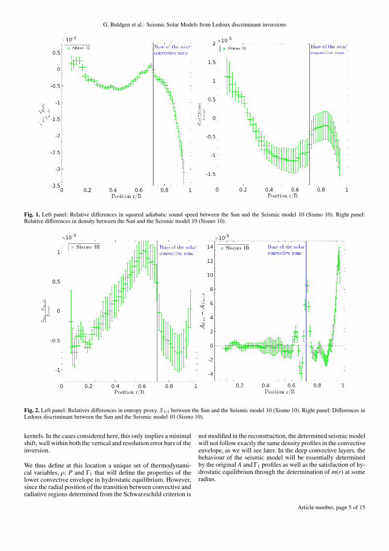
In the convective zone, no correction to the A profile is appliedas the inversion results are not trustworthy. Indeed, the inversionhas a tendency to overestimate the amplitude of the correctionsin a region where A is very small, as a consequence of the lowamplitude of both chemical gradients and departures from theadiabatic temperature gradient in the lower parts of the convec-tive zone. Consequently, the corrections in the convective zoneare actually implicitly applied when the structure is reintegratedto satisfy hydrostatic equilibrium with the boundary conditionson M and R. Thus, despite not directly correcting the structuralvariables in the convective zone with the inversion, we are stillable to significantly improve the agreement of sound speed, den-sity, Ledoux discriminant and entropy proxy inversions for thereconstructed models, as illustrated in the left and right panelsof Figs. 1 and 2 for Model 10 after 7 iterations.

As we mentioned above, the reconstruction procedure does notexplicitly apply corrections in A in the convective layers. Thismeans that the corrections in these regions are a sole conse-quence of the modifications required to satisfy mass conser-vation in the reconstructed models. As we will see in Sect.3.1 when looking at the changes in squared adiabatic soundspeed at each iteration, the agreement in the convective enve-lope for this specific quantity is actually not improved over thereconstruction procedure. Consequently, it is clear that our seis-mic models do not provide an as good agreement in adiabaticsound speed in those regions as those determined in previousstudies explicitly correcting the profiles in the convective en-velope (see e.g. Antia & Basu 1994b; Turck-Chièze et al. 2004;Vorontsov et al. 2014). This is a direct consequence of our re-construction method, for which we chose to focus on the deeperradiative layers, where the uncertainties on Γ1 are much smaller.Thus, in comparison to previous studies, our models performvery well in the deeper layers, especially for the density pro-file. This improvement of the density and entropy proxy profilesover the course of the iterations is a direct consequence of themass conservation. Indeed, even if the convective layers are leftuntouched, the variations of density resulting from the A cor-rections applied in the radiative interior will be compensated bylarger variations in the upper, less-dense, convective layers, lead-ing to an improvement of the agreement with the Sun for bothdensity and entropy proxy.

At the exact location of the BCZ, the corrections to the Ledouxdiscriminant are still applied, using the δA amplitude given bythe inversion point with the closest central value of the averaging



Fig. 1. Left panel: Relative differences in squared adiabatic sound speed between the Sun and the Seismic model 10 (Sismo 10). Right panel:Relative differences in density between the Sun and the Seismic model 10 (Sismo 10).

Fig. 2. Left panel: Relatives differences in entropy proxy, S 5/3 between the Sun and the Seismic model 10 (Sismo 10). Right panel: Differences inLedoux discriminant between the Sun and the Seismic model 10 (Sismo 10).

kernels. In the cases considered here, this only implies a minimalshift, well within both the vertical and resolution error bars of theinversion.

We thus define at this location a unique set of thermodynami-cal variables, ρ, P and Γ1 that will define the properties of thelower convective envelope in hydrostatic equilibrium. However,since the radial position of the transition between convective andradiative regions determined from the Schwarzschild criterion is

not modified in the reconstruction, the determined seismic modelwill not follow exactly the same density profiles in the convectiveenvelope, as we will see later. In the deep convective layers, thebehaviour of the seismic model will be essentially determinedby the original A and Γ1 profiles as well as the satisfaction of hy-drostatic equilibrium through the determination of m(r) at someradius.



Another region left untouched in the reconstruction procedureare the surface layers of the model, namely the substantiallysuper-adiabatic convective layers as well as the atmosphere. Thischoice is justified by the fact that inversions based on the varia-tional principle of adiabatic stellar oscillations are unable to pro-vide reliable constraints in these regions; thus the inferred cor-rections would not be appropriate. This also justifies the use ofdifferent atmosphere models and formalisms of convection, aswe can then directly measure their impact on the final recon-structed structure of the Sun (see Sect. 4).

In the right panel Fig. 3, we illustrate the convergence of thereconstruction procedure for Model 10. The final agreement inLedoux discriminant inversions for all models in our sample isillustrated in the left panel of Fig. 3 and a selection of the corre-sponding Ledoux discriminant profiles are illustrated in Fig. 8.As can be seen, the agreement is excellent in the deep radiativelayer, whatever the initial conditions. Small discrepancies canbe seen just below the BCZ at the resolution limit of the SOLAinversion. The central regions (below 0.08 R⊙) are also slightlydifferent, since they are not modified during the reconstructionprocedure.

From the analysis of the Ledoux discriminant inversions, we canconclude that the reconstruction procedure has been able to pro-vide a precise, model-independent profile of this quantity in theSun which can be used to analyse the limitations of the currentmodels. As mentioned previously, another key aspects for futureadvances in helioseismology is the potential observation of grav-ity modes. Below ≈ 200 µHz, the gravity modes follow a regularpattern and are described to the first order by an asymptotic ex-pression as a function of their period, Pn,ℓ

Pn,ℓ =P0√ℓ(ℓ + 1)

(n + ℓ/2 + υ) , (5)

with n the radial order, ℓ the degree, υ a phase shift dependingon the properties near the BCZ and P0 is defined by

P0 =2π2

∫ rBCZ

0(N/r) dr

=2π2

∫ rBCZ

0

√

|gA/r2|dr, (6)

with N the Brunt-Väisälä frequency and rBCZ the radial positionof the BCZ. This implies that the separation between two modesof consecutive n in the asymptotic regime, denoted the asymp-totic period spacing, is determined by P0 (i.e. by the integral ofthe Brunt-Väisälä frequency up to the BCZ).

We illustrate the results of these integrals of P0 for our seismicand reference models in Table 2, which shows that despite hav-ing good constraints on the Ledoux discriminant in the deep ra-diative layer of the Sun, the fact that we are missing the deepcore still allows for a significant variation of the period spacingof g-modes in our sample of reconstructed structures. Typically,we find a range of period spacing values spanning an intervalof 25 s far from the observed value of 2040 s of Fossat et al.(2017) but closer to the theoretical one of 2105 s of Provost et al.(2000). Only slight changes in the period spacing values, of theorder of 10 s, are found if the reconstruction procedure is carriedout using GOLF data from Salabert et al. (2015) instead of Bi-SON data for the low degree modes. However, these determinedvalues can be significantly changed by altering the A profile be-low 0.08 R⊙ without destroying the agreement with the inversionresults from p-modes. Hence, another input is required to betterconstrain the expected period spacing of the solar gravity modes.

Table 2. Comparison between period spacing values for the seismicmodels after 7 iterations and the reference models values.

Name P0 (s) P0,Ref (s)

Sismo 1 2162 2162Sismo 2 2161 2138Sismo 3 2157 2157Sismo 4 2170 2186Sismo 5 2175 2207Sismo 6 2176 2199Sismo 7 2155 2160Sismo 8 2164 2163Sismo 9 2153 2188

Sismo 10 2164 2164

This will be further discussed in Sect. 4 when studying the im-pact of the choice of the reference model.

3. Agreement with other seismic indices

In the previous section, we focused on demonstrating that usingsuccessive inversions of the Ledoux discriminant allowed us todetermine a model-independent profile for this quantity. How-ever, the main benefit of the reconstruction procedure is that itallows to determine fully consistent seismic models of the solarstructure, that are also in excellent agreement in terms of otherstructural variables. In this section, we will show that once the re-construction procedure has converged, we reach a level of agree-ment in the radiative zone of ≈ 0.1% for structural inversions ofρ, c2 and S 5/3 = P/ρ5/3. This implies that most of the issues withour depiction of the solar structure are clearly related to the ra-diative layers, as we are able to suppress efficiently other tracesof mismatches by correcting A in the radiative region.

3.1. Sound-speed inversions

The sound-speed inversions are carried out using the (c2, ρ) ker-nels in Eq. (3). As can be seen from the left panel of Fig. 4, theagreement for all models is of ≈ 0.1% in the radiative region andthe lower parts of the convective region. From the right panel of4, we also see that, as mentioned earlier, the sound speed profilein the convective envelope is not corrected by the reconstructionprocedure, as no corrections in A are applied in the convectiveenvelope.

These results confirm that, as expected, the solar modelling prob-lem is mostly an issue related to the temperature gradient of thelow-metallicity models in the radiative regions. However, fromthe analysis of the successive changes due to the iterations in thereconstruction procedure, illustrated in the right panel of Fig. 4,we can see that the bulk of the profile is corrected after the thirdreconstruction. The first step mostly corrects the sound-speeddiscrepancy in the radiative zone, near the BCZ. The remainingdiscrepancies are efficiently corrected in the following iterations.However, one can see that there is a remaining discrepancy evenfor the model obtained after 7 iteration. These variations remainvery small and are not linked to significant deviations in the Aprofile. They do not seem to be linked to Γ1 differences betweenthe models, but rather to the position of the BCZ and the masscoordinate at that position. Indeed, these parameters determinethe density profile of the models and it is clear that the models



Fig. 3. Left panel: Illustration of the agreement in Ledoux discriminant for the reconstructed models using the reference models of Table 1 asinitial conditions. Right panel: Illustration of the convergence of the A corrections for successive iterations of the reconstruction procedure in thecase of Model 10.

Fig. 4. Left panel: Agreement in relative sound-speed differences for the reconstructed models using the reference models of Table 1 as initialconditions. Right panel: Illustration of the convergence of the sound speed relative differences for successive iterations of the reconstructionprocedure in the case of Model 10.

with the worst agreement on the position of the BCZ with re-spect to the helioseismic value of 0.713±0.001 R⊙ also have thelargest discrepancies in both sound-speed and, as shown in Sect.3.3, density profiles. This implies that an additional selection ofthe models based on their position of the BCZ and the mass coor-dinate at the BCZ could be used as a second step. Unfortunately,we do not have a direct measurement of the mass coordinateat the BCZ. Vorontsov et al. (2014) were able to determine themass coordinate at 0.75R⊙, m0.75 = 0.9822 ± 0.0002 M⊙ anddiscussed its importance as a calibrator of the specific entropy

in the solar convective envelope. All our reconstructed modelsare in good agreement with the determined value of the m0.75

parameter of Vorontsov et al. (2014), as illustrated in Table 3.Similarly, they all show very good agreement in entropy proxyinversions as we will further discuss in Sec. 3.2.



Table 3. Comparison between m0.75 for the seismic models after 7 iter-ations and their corresponding reference models values

Name m0.75 m0.75,Ref

Sismo 1 0.9823 0.9826Sismo 2 0.9823 0.9822Sismo 3 0.9824 0.9820Sismo 4 0.9823 0.9832Sismo 5 0.9823 0.9834Sismo 6 0.9823 0.9836Sismo 7 0.9824 0.9822Sismo 8 0.9824 0.9826Sismo 9 0.9823 0.9826

Sismo 10 0.9823 0.9826

3.2. Entropy proxy inversions

The entropy proxy inversions are carried out using the(S 5/3, Γ1) kernels in Eq. (3). These kernels have been pre-sented in Buldgen et al. (2017a) and applied to the solar case inBuldgen et al. (2017d) and Buldgen et al. (2019). From the leftpanel of Fig. 5, we can see that the agreement for this inver-sion is also of ≈ 0.1% in the radiative and convective regions forall models, whatever their initial conditions. This confirms thatcorrecting for the A profile in the radiative region leads to an ex-cellent agreement of the height of the plateau in the convectivezone.

From a closer analysis of the reconstruction procedure, we cansee that a good agreement of the height of the plateau is reachedafter 3 iterations. The explanation for this is found in the formof the applied corrections to the model. At first, the reconstruc-tion procedure is dominated by the large discrepancies near theBCZ in all models. Once these differences have been partiallycorrected, we can see in the right panel of Fig. 5 that the correc-tions in the deeper layer of the radiative zone remain significantfor the second iteration. It then takes 2 iterations to completelyerase discrepancies in the A profile below 0.6 R⊙. Once this isachieved, the inferred A profile shows an oscillatory behaviourin these regions (as seen in Fig. 3). This phenomenon is linked toa form of Gibbs phenomenon, due to the fact that the remainingdeviations are located in very narrow region, just below the BCZand are too sharp to be properly sampled by the classical SOLAmethod we use in this study. From a physical point of view, theremaining discrepancies may originate from multiple contribu-tions: a slight mismatch between the transition from the radiativeto convective outward transport of energy, which causes a sharpvariation in A and a mismatch in A in the last percent of solarradii just below the BCZ. Of course, it should be recalled that abreaking of spherical symmetry in the structure of the tachoclineregion could also lead to mismatches with any modelling assum-ing spherical symmetry.

3.3. Density inversions

The density inversions have been carried out using the (ρ, Γ1)structural kernels, ensuring that the total solar mass is conservedduring the inversion procedure. By using the (ρ, Γ1) kernels, weensure an intrinsically low contribution of the cross-term, as therelative variations of Γ1 are expected to be very small in most ofthe solar structure. The inversion results for all models are illus-trated in the left panel of Fig. 6. From these results, it appears

that most of the models show an excellent agreement in density,of around 0.2% in the radiative layers. The best models showan agreement below 0.1% throughout most of the solar structureand the worst offenders showing discrepancies as high as 0.25%in the deep layers. These are also the models showing the largediscrepancies in sound speed discussed earlier and thus, the dis-agreements we find are actually due to the fact that these modelsdo not fit at best the position of the base of the convective zoneof 0.713 ± 0.001 R⊙. As discussed in Sect. 3.1, this means thata second selection can be performed based on the position ofthe BCZ. This, however, does not have any implication regard-ing abundances but solely constrains further the behaviour of theLedoux discriminant around the BCZ and thus has strong im-plications on the properties of the macroscopic mixing in thoselayers. However, due to the lack of resolution in the inversionprocedure, a definitive answer at the BCZ will likely be the re-sult of non-linear inversions adapted to sample steep gradientsof the function to be determined from the seismic data.

Taking a look at the right panel of Fig. 6, we can see that thefirst reconstruction step leads to a significant improvement of thedensity profile. Unlike the sound-speed inversion, the second andthird step lead to smaller improvement of the inversion results inradiative layers. This is also seen in the entropy proxy inversion,where the leap after the first reconstruction step is mainly dueto the corrections of the discrepancies around 0.6 R⊙ but provid-ing a better overall agreement in the radiative region is mainlydue to finer corrections at higher temperatures. This also consis-tent with the results of Buldgen et al. (2019), where a localizedchange of the mean Rosseland opacity could provide some im-provement in sound speed and Ledoux discriminant, but was notenough to provide an excellent agreement regarding the entropyproxy inversion.

3.4. Frequency-separation ratios

As a last verification step of the reconstruction procedure, wetake a look at the so-called frequency-separation ratios defined inRoxburgh & Vorontsov (2003) of the 6 of our reconstructed solarmodels. These quantities are defined as the ratio of the so-calledsmall frequency separation over the large frequency separationratio as follows

r02 =ν0,n − ν2,n−1

ν1,n − ν1,n−1

(7)

r13 =ν1,n − ν3,n−1

ν0,n+1 − ν0,n, (8)

with νℓ,n the frequency of radial order n and degree ℓ.

In Fig. 7, we plot the difference between the observed frequency-separation ratios and those of our seismic models, normalized bytheir 1σ uncertainties. As can be seen, the agreement for all mod-els is excellent. From the comparison with the results of Model1 in blue, we can see that the improvement in the agreementis quite significant. This is no surprise, as the reconstruction isbased on reproducing the Ledoux discriminant inversions, whichis closely linked to the sound-speed gradient and thus to thefrequency-separation ratios, following the asymptotic develop-ments of Shibahashi (1979) and Tassoul (1980). This also meansthat the frequency-separation ratios, just as any other classic he-lioseismic investigation such as structural inversions, are by nomeans direct measurement of the chemical abundances in thedeep radiative layers. As a consequence, they cannot be used to



Fig. 5. Left panel: Agreement in relative entropy proxy differences for the reconstructed models using the reference models of Table 1 as initialconditions. Right panel: Illustration of the convergence of the entropy proxy relative differences for successive iterations of the reconstructionprocedure in the case of Model 10.

0 0.2 0.4 0.6 0.8 1

-5

-4

-3

-2

-1

0

1

2

10 -3

0 0.2 0.4 0.6 0.8 1-5

0

5

10

15

2010 -3

Fig. 6. Left panel: Agreement in relative density differences for the reconstructed models using the reference models of Table 1 as initial conditions.Right panel: Illustration of the convergence of the density relative differences for successive iterations of the reconstruction procedure in the caseof Model 10.

advocate the use of one or the other abundance table for the con-struction of solar models.

4. Impact of reference models

While the reconstruction procedure leads to a very similarLedoux discriminant profile for a wide range of initial modelproperties, it might not be fully justified to say that it is com-pletely independent of the initial conditions of the procedure. In

the previous sections, we have discussed how the position of theBCZ could affect the final agreement for sound-speed, densityand entropy proxy inversions.

However, this is an impact that can be easily measured from thecombination of multiple structural inversions and lead to someextent to an additional selection of the optimal seismic struc-ture of the Sun. Other effects, such as the selected dataset or theassumed behaviour of the surface correction may lead to slightdifferences at the level of agreement we seek with such recon-



1500 2000 2500 3000 3500-14

-12

-10

-8

-6

-4

-2

0

2

4

6

1500 2000 2500 3000 3500-12

-10

-8

-6

-4

-2

0

2

4

Fig. 7. Agreement in frequency-separation ratios of low-degree p-modes for 6 reconstructed models using the corresponding references of Table 1as initial conditions as well as reference Model 1 shown as comparison.

struction procedure. Using for example an extended MDI datasetsuch as the one of Reiter et al. (2015, 2020) may provide waysto further test the robustness of our procedure, as well as betterprobe the agreement of our seismic model of the Sun in the con-vective envelope. Indeed, from the comparison of models Sismo1, Sismo 8 and Sismo 9, we can see that some small variationsin the upper envelope properties remain after the reconstructionprocedure. The changes in the radiative region between thesemodels are unsurprisingly much more smaller. This implies thatadditional insight can be gained from using an extended datasetprobing in a more stringent manner the upper convective layers,as in Di Mauro et al. (2002); Vorontsov et al. (2013).

The approach used to connect the regions on which the A correc-tions are applied to the central regions may also locally impactthe procedure. Obviously, the fact that no corrections are appliedbelow 0.08 R⊙ leaves a direct mark on the final reconstructedstructure. This is illustrated in Fig. 8 and Fig 9 where we plot theLedoux discriminant, Brunt-Väisälä frequency and sound-speedprofiles of all our reconstructed models in the deep solar core.From the inspection of the right panel of Fig. 8, we can under-stand better the behaviour of the period spacing changes of table2. Indeed, Model 1 and 7 show some minor changes in asymp-totic period spacing, while the spacing of Model 5 is significantlycorrected. This is simply due to the fact that Model 1 and 7 re-produce much better the Brunt-Väisälä frequency of the Sun inthe deep radiative layers. However, as we lack constraints below0.08 R⊙, we cannot state with full confidence that the observedperiod spacing will lay within the 25 s range we find.

The optimal approach to lift the degeneracy in the inner corewould be to have at our disposal an observed value of the pe-riod spacing of the solar gravity modes. Including constraintsfrom neutrino fluxes may already provide additional constraints.However, their main limitation is that in this case, we wouldhave to assume a given composition profile for our solar mod-

els, a given equation of state as well as nuclear reaction rates.Taking these constraints into account implies that we use allour current knowledge on the present day solar structure. How-ever, this would be at the expense of adding more uncertain-ties and "model-dependencies" in the procedure. In their paper,Shibahashi & Takata (1996) only made an assumption on Z(r),the distribution of heavy element in the solar interior, but theysolved the equation of radiative transfer and thus assumed themean Rosseland opacity to be known. Given the current uncer-tainties on radiative opacities, it might be safer to avoid such anassumption, especially at lower temperatures.

Unravelling the core properties of the Sun would be crucialfor the theory of stellar physics. First, it would allow to con-strain the angular momentum transport processes acting in so-lar and stellar radiative zones, as discussed in Eggenberger et al.(2019). Second, it would demonstrate whether the solar corehas undergone intermittent mixing, for example due to out-of-equilibrium burning of 3He (Dilke & Gough 1972; Unno 1975;Gabriel et al. 1976) or a prolongated lifetime of its transitoryconvective core in the early main-sequence evolution. Third,it would also allow us to constrain nuclear reactions rates andtheir screening factors, as these remain key ingredients of stellarmodels that are quite uncertain from a theoretical point of view(see e.g. Mussack & Däppen 2011; Mussack 2011, for a discus-sion).

5. Limitations and uncertainties

From the previous sections, we have demonstrated how the in-version of the Ledoux discriminant can be used to build a seismicSun from successive correction, integration and inversion steps.While the process is quite straightforward and allows us to testthe consistency between different inversions of the solar struc-ture it also suffers from intrinsic limitations.



Fig. 8. Left panel: Ledoux discriminant profiles from the reconstruction procedure. The dashed lines illustrate the reference profile of some of themodels in Table 1 while the continuous lines show the profile on which the procedure converges (using all reference models). Right panel: Sameas the left panel but for the Brunt-Väisälä frequency.

0 0.02 0.04 0.06 0.08 0.12.54

2.55

2.56

2.57

2.58

2.59

2.6

2.61

10 15

Fig. 9. Sound-speed profile in the core region of the reconstructedmodel, showing the impact of initial conditions in the deep solar core,that is unconstrained by p modes.

The first limitation is due to the incomplete information givenby the inversion technique. Indeed, since p-modes do not allowus to test solar models below 0.08 R⊙, we are not able to get afull view of the seismic Sun. While it only represents 8% of thesolar structure in radial extent, it also represents≈ 3% in mass ofthe solar structure, which actually corresponds to the total massof the solar convective envelope. This implies that an accuratedepiction of the mass distribution inside the Sun can only behoped for if we observe solar g modes. This is also illustratedfrom the results of Table 2 which shows that the reconstruction

only slightly alters the values of the period spacing. Obtaininga precise measurement of that quantity would indeed providea strong additional selection on the set of seismic models andallow for joint analyses using both neutrino fluxes measurementand helioseismology.

The second main limitation also stems from the inversion pro-cedure and is linked to the impact of the surface effects. Indeed,as can be seen from sound-speed, entropy proxy and density in-versions, the upper layer of the model have not been extensivelyprobed by the inversion procedure. As we only apply correc-tions in A in the internal radiative layers, this does not render thereconstruction procedure useless. However, this means that theconclusions we can draw from the other inversion proceduresused as sanity checks are mostly limited to the lower parts ofthe envelope and the radiative region. This implies that to betterconstrain the properties of the solar convective envelope (com-position, equation of state, ...), we will have to extend the datasetto higher degree modes. Of course, this means that we will haveto be more attentive to the surface effects that can lead to bi-ases in the determined corrections from these higher frequencymodes (see e.g. Gough & Vorontsov 1995).

Not applying the corrections in the convective envelope is alsoa clear limiting factor of our method. While the improvement issignificant when comparing the initial models in terms of densityand entropy proxy profile, it is also clear that the sound speedprofile in the convective envelope is not extensively corrected byour method. This leads our seismic models to be somewhat lessperformant in terms of sound speed in the convective envelope,while being more performant in the radiative region, especiallyregarding density and entropy proxy inversions. Consequently, apromising way of obtaining a very accurate picture of the inter-nal structure of the Sun from helioseismology would be to com-bine our reconstruction technique with those focusing on obtain-



ing optimal models of the solar convective envelope (as shownfor example in Vorontsov et al. 2014).

In addition to these limitations that are intrinsic to the use ofseismic inversions from solar acoustic oscillations, we have alsomade the hypothesis to keep the Γ1 profile and the position ofthe BCZ unchanged in the reconstruction procedure. The BCZposition is not a strong limitation, as it can easily be avoided byensuring that the reference model agrees with the helioseismi-cally determined value. As we have seen from Fig. 8, this has noimpact on the final Ledoux discriminant profile determined bythe reconstruction procedure.

The hypothesis of unchanged Γ1 can be more severe if we startlooking at changes in the thermodynamical quantities of smallamplitude. Indeed, Vorontsov et al. (2014) have reported mea-

surements of the δΓ1

Γ1profile of a precision of up to 10−4 in the

deepest half part of the convection zone, which is just one or-der of magnitude bigger than the estimated precision of equationof state interpolation routines (Baturin et al. 2019). This impliesthat at the magnitude of the relative differences we see in the so-lar convective envelope, keeping Γ1 constant might not be a goodstrategy, but also that we have to become attentive to the intrin-sic numerical limitations of the tabulated ingredients of our solarmodels.

Moreover, intrinsic changes between different equations of statewill necessarily lead to slight differences in the determined pro-files. Since the Γ1 profile in the convective envelope is stronglytied to the assumed chemical composition of the envelope, thisalso means that the properties of the envelope of our seismicmodels may not be fully consistent. Indeed, the density, pres-sure and Γ1 profiles are determined (or fixed) in our approach.Providing consistent profiles of X, Z and T for the reconstructedstructure might very likely require to assume changes in Γ1 in theenvelope of our models. This is beyond the scope of this study,but will be addressed in the future using the most recent versionsof equations of state available (Baturin et al. 2013) using Γ1 in-versions in the solar envelope.

In the radiative layers, the hypothesis of unchanged Γ1 is lessconstraining, as one can safely assume that the A correctionswill be largely dominated by the contributions from the pressureand density gradients. However, there is still a degeneracy be-tween temperature and chemical composition, that can both leadto changes in pressure and density profiles, even if an equation ofstate is assumed. This is also a clear limitation of our procedure,but is intrinsic to its seismic nature.

A third limitation of our reconstruction is also linked to the seis-mic data used. We carried out additional tests using MDI datafrom Larson & Schou (2015) and from the latest release fol-lowing the fitting methodology of Korzennik (2005), Korzennik(2008a) and Korzennik (2008b) as well as GOLF data instead ofBiSON data for the low degree modes and found that variationsof up to ≈ 3 × 10−3 could be found in the sound speed pro-files of the seismic models, while using the latest MDI datasetsled to changes of about ≈ 1 × 10−3 and using GOLF data from(Salabert et al. 2015) instead of BiSON data led to similar devia-tions. The largest differences were however found below 0.08R⊙,in a region uncontrolled by the reconstruction procedure. Thisimplies that the actual accuracy of the reconstruction is tightlylinked to the dataset used.

6. Conclusion

We have presented a new approach to compute a seismic Sun,taking advantage of the Ledoux discriminant inversions to limitthe amount of numerical differentations when computing the so-lar structure. Our approach allows us to provide a full profile ofthe Ledoux discriminant for our seismic models. To verify theconsistency and robustness of our method, we have checked thatit also led to an improvement of other classical helioseismic indi-cators such as frequency-separation ratios as well as other struc-tural inversions. By selecting models with the exact position ofthe discontinuity in A determined by helioseismology, the recon-structed models agree with the Sun well within 0.1% for all otherstructural inversions in the radiative interior. Slightly larger dif-ferences can be seen depending on the dataset used to carry outthe reconstruction.

Our procedure converges consistently on a unique estimate ofthe solar Ledoux discriminant within the range of radii on whichthe inversions are considered reliable. This approach opens newways of analysing the current uncertainties on the solar tempera-ture gradient, as the main advantage of the Ledoux discriminantis that it is largely dominated by the contribution of the differ-ence between the temperature gradient and the adiabatic tem-perature gradient in most of the radiative zone. This opens upthe possibility to estimate directly the expected opacity modifi-cation for a given equation of state and a given chemical compo-sition, providing key insights to the opacity community (see alsoGough 2004). This approach provides a complementary way toestimate the required modifications expected to be a key elementin solving the current stalemate regarding the solar abundancesfollowing their revision by Asplund et al. (2009).

In the regions where the mean molecular weight term of Ahas a non-negligible contribution (close to the BCZ and in re-gions affected by nuclear reactions), further degeneracies can beexpected and thus larger uncertainties. However, by analysingthese effects, we can expect to gain insights on the properties ofmicroscopic diffusion and mixing at the BCZ. Gaining more in-sights on the behaviour of the discontinuity in the A profile in thetachocline region will require using one of our seismic modelsas a reference for non-linear RLS inversions as in Corbard et al.(1999), allowing for solutions of the inversion displaying largergradients. This will be done in future studies.

In the convective envelope, the reconstruction procedure allowsto set a good basis for precise determinations of the composi-tion in this region, especially for Z, improving on Buldgen et al.(2017c), and tests of the equation of state used in solar and stellarmodels. Indeed, this requires to avoid as much as possible con-taminations by the unavoidable cross-term contributions whilestill being able to test different equations of states. By usinghigher ℓ modes (Reiter et al. 2015, 2020), we can expect to fur-ther test the robustness of our approach in the convective enve-lope and provide estimates of the physical properties of the Sunin this region.

Gaining more information on the solar core will very likelybe more difficult, as the procedure is intrinsically limited bythe solar p-modes. However, combining it with neutrino fluxesmay provide a way to further constrain the solar structure. Inaddition, it may also be useful to predict the expected rangeof the asymptotic value of the period spacing of g-modes,helping with their detection. This is particularly timely, giventhe recent discussions in the literature about the potential de-tection of these modes (Fossat et al. 2017; Fossat & Schmider



2018; Schunker et al. 2018; Appourchaux & Corbard 2019;Scherrer & Gough 2019) and the renewed interest it inspiredfor the quest to find them. Should this additional seismic con-straint become available, it could be easily included in the pro-cedure and open a new era of solar physics. As such, the Sunstill remains an excellent laboratory of fundamental physics andthe current study provides a new, original way to exploit theinformation available from the observation of acoustic oscilla-tions.

Acknowledgements

We thank the referee for the useful comments that have sub-stantially helped to improve the manuscript. G.B. acknowledgesfundings from the SNF AMBIZIONE grant No 185805 (Seis-mic inversions and modelling of transport processes in stars).P.E. and S. J. A. J. S. have received funding from the EuropeanResearch Council (ERC) under the European Union’s Horizon2020 research and innovation programme (grant agreement No833925, project STAREX). This article used an adapted ver-sion of InversionKit, a software developed within the HELASand SPACEINN networks, funded by the European Commis-sions’s Sixth and Seventh Framework Programmes. Funding forthe Stellar Astrophysics Centre is provided by The Danish Na-tional Research Foundation (Grant DNRF106). We acknowledgesupport by the ISSI team “Probing the core of the Sun and thestars” (ID 423) led by Thierry Appourchaux.

References

Adelberger, E. G., García, A., Robertson, R. G. H., et al. 2011, Reviews of Mod-ern Physics, 83, 195

Antia, H. M. & Basu, S. 1994a, ApJ, 426, 801Antia, H. M. & Basu, S. 1994b, A&Aps, 107, 421Antia, H. M. & Basu, S. 2005, ApJ, 620, L129Appourchaux, T. & Corbard, T. 2019, A&A, 624, A106Asplund, M., Grevesse, N., Sauval, A. J., & Scott, P. 2009, ARA&A, 47, 481Ayukov, S. V. & Baturin, V. A. 2011, in Journal of Physics Conference Series,

Vol. 271, Journal of Physics Conference Series, 012033Ayukov, S. V. & Baturin, V. A. 2017, Astronomy Reports, 61, 901Bailey, J. E., Nagayama, T., Loisel, G. P., et al. 2015, Nature, 517, 3Basu, S. & Antia, H. M. 1995, MNRAS, 276, 1402Basu, S. & Antia, H. M. 1997, MNRAS, 287, 189Basu, S. & Antia, H. M. 2008, Phys. Rep., 457, 217Basu, S., Chaplin, W. J., Elsworth, Y., New, R., & Serenelli, A. M. 2009, ApJ,

699, 1403Basu, S. & Thompson, M. J. 1996, A&A, 305, 631Baturin, V. A., Ayukov, S. V., Gryaznov, V. K., et al. 2013, in Astronomical

Society of the Pacific Conference Series, Vol. 479, Progress in Physics of theSun and Stars: A New Era in Helio- and Asteroseismology, ed. H. Shibahashi& A. E. Lynas-Gray, 11

Baturin, V. A., Däppen, W., Oreshina, A. V., Ayukov, S. V., & Gorshkov, A. B.2019, A&A, 626, A108

Benomar, O., Takata, M., Shibahashi, H., Ceillier, T., & García, R. A. 2015,MNRAS, 452, 2654

Bergemann, M. & Serenelli, A. 2014, Solar Abundance Problem, in Determina-tion of Atmospheric Parameters of B-, A-, F- and G-Type Stars: Lectures fromthe School of Spectroscopic Data Analyses, ed. E. Niemczura, B. Smalley, &W. Pych (Cham: Springer International Publishing), 245–258

Blancard, C., Colgan, J., Cossé, P., et al. 2016, Physical Review Letters, 117,249501

Brown, T. M. & Morrow, C. A. 1987, in Astrophysics and Space Science Library,Vol. 137, The Internal Solar Angular Velocity, ed. B. R. Durney & S. Sofia,7–17

Buldgen, G., Reese, D. R., & Dupret, M. A. 2017a, A&A, 598, A21Buldgen, G., Salmon, S. J. A. J., Godart, M., et al. 2017b, MNRAS, 472, L70Buldgen, G., Salmon, S. J. A. J., Noels, A., et al. 2019, arXiv e-prints,

arXiv:1902.10390Buldgen, G., Salmon, S. J. A. J., Noels, A., et al. 2017c, MNRAS, 472, 751

Buldgen, G., Salmon, S. J. A. J., Noels, A., et al. 2017d, A&A, 607, A58Canuto, V. M., Goldman, I., & Mazzitelli, I. 1996, ApJ, 473, 550Canuto, V. M. & Mazzitelli, I. 1991, ApJ, 370, 295Canuto, V. M. & Mazzitelli, I. 1992, ApJ, 389, 724Charbonnel, C. & Talon, S. 2005, Science, 309, 2189Christensen-Dalsgaard, J., Duvall, T. L., J., Gough, D. O., Harvey, J. W., &

Rhodes, E. J., J. 1985, Nature, 315, 378Christensen-Dalsgaard, J., Gough, D. O., & Knudstrup, E. 2018, MNRAS, 477,

3845Christensen-Dalsgaard, J., Gough, D. O., & Thompson, M. J. 1991, ApJ, 378,

413Christensen-Dalsgaard, J. & Houdek, G. 2010, Ap&SS, 328, 51Christensen-Dalsgaard, J., Thompson, M. J., & Gough, D. O. 1989, MNRAS,

238, 481Colgan, J., Kilcrease, D. P., Magee, N. H., et al. 2016, ApJ, 817, 116Corbard, T., Blanc-Féraud, L., Berthomieu, G., & Provost, J. 1999, A&A, 344,

696Cox, J. & Giuli, R. 1968, Principles of Stellar Structure: Applications to stars

(Gordon and Breach)Davies, G. R., Broomhall, A. M., Chaplin, W. J., Elsworth, Y., & Hale, S. J. 2014,

MNRAS, 439, 2025Deheuvels, S., Dogan, G., Goupil, M. J., et al. 2014, A&A, 564, A27Deheuvels, S., García, R. A., Chaplin, W. J., et al. 2012, ApJ, 756, 19Di Mauro, M. P., Christensen-Dalsgaard, J., Rabello-Soares, M. C., & Basu, S.

2002, A&A, 384, 666Dilke, F. W. W. & Gough, D. O. 1972, Nature, 240, 262Dziembowski, W. A., Pamiatnykh, A. A., & Sienkiewicz, R. . 1991, MNRAS,

249, 602Dziembowski, W. A., Pamyatnykh, A. A., & Sienkiewicz, R. 1990, MNRAS,

244, 542Eggenberger, P., Buldgen, G., & Salmon, S. J. A. J. 2019, A&A, 626, L1Eggenberger, P., Maeder, A., & Meynet, G. 2005, A&A, 440, L9Elliott, J. R. 1996, MNRAS, 280, 1244Ferguson, J. W., Alexander, D. R., Allard, F., et al. 2005, ApJ, 623, 585Fossat, E., Boumier, P., Corbard, T., et al. 2017, A&A, 604, A40Fossat, E. & Schmider, F. X. 2018, A&A, 612, L1Gabriel, M., Noels, A., Scuflaire, R., & Boury, A. 1976, A&A, 47, 137Gough, D. 2004, in American Institute of Physics Conference Series, Vol. 731,

Equation-of-State and Phase-Transition in Models of Ordinary AstrophysicalMatter, ed. V. Celebonovic, D. Gough, & W. Däppen, 119–138

Gough, D. O. & Kosovichev, A. G. 1993, MNRAS, 264, 522Gough, D. O. & McIntyre, M. E. 1998, Nature, 394, 755Gough, D. O. & Scherrer, P. H. 2001, The solar interior, in The Century of Space

Science, ed. J. A. M. Bleeker, J. Geiss, & M. C. E. Huber (Dordrecht: SpringerNetherlands), 1035–1063

Gough, D. O. & Vorontsov, S. V. 1995, MNRAS, 273, 573Grevesse, N. & Noels, A. 1993, in Origin and Evolution of the Elements, ed.

N. Prantzos, E. Vangioni-Flam, & M. Casse, 15–25Gryaznov, V., Iosilevskiy, I., Fortov, V., et al. 2013, Contributions to Plasma

Physics, 53, 392Gryaznov, V. K., Ayukov, S. V., Baturin, V. A., et al. 2004, in American In-

stitute of Physics Conference Series, Vol. 731, Equation-of-State and Phase-Transition in Models of Ordinary Astrophysical Matter, ed. V. Celebonovic,D. Gough, & W. Däppen, 147–161

Gryaznov, V. K., Ayukov, S. V., Baturin, V. A., et al. 2006, Journal of Physics A:Mathematical and General, 39, 4459

Guzik, J. A. & Mussack, K. 2010, ApJ, 713, 1108Guzik, J. A., Watson, L. S., & Cox, A. N. 2006, Mem. Soc. Astron. Italiana, 77,

389Howe, R. 2009, Living Reviews in Solar Physics, 6, 1Iglesias, C. A. 2015, MNRAS, 450, 2Iglesias, C. A. & Hansen, S. B. 2017, ApJ, 835, 284Iglesias, C. A. & Rogers, F. J. 1996, ApJ, 464, 943Irwin, A. W. 2012, FreeEOS: Equation of State for stellar interiors calculations,

Astrophysics Source Code LibraryKorzennik, S. G. 2005, ApJ, 626, 585Korzennik, S. G. 2008a, Astronomische Nachrichten, 329, 453Korzennik, S. G. 2008b, in Journal of Physics Conference Series, Vol. 118, Jour-

nal of Physics Conference Series, 012082Kosovichev, A. G. 1993, MNRAS, 265, 1053Kosovichev, A. G. 1999, Journal of Computational and Applied Mathematics,

109, 1Kosovichev, A. G. 2011, Advances in Global and Local Helioseismology: An

Introductory Review, in Lecture Notes in Physics, Berlin Springer Verlag, ed.J.-P. Rozelot & C. Neiner, Vol. 832, 3

Kosovichev, A. G. & Fedorova, A. V. 1991, Soviet Ast., 35, 507Krishna Swamy, K. S. 1966, ApJ, 145, 174Landi, E. & Testa, P. 2015, ApJ, 800, 110Larson, T. P. & Schou, J. 2015, Sol. Phys., 290, 3221Lund, M. N., Miesch, M. S., & Christensen-Dalsgaard, J. 2014, ApJ, 790, 121



Marchenkov, K., Roxburgh, I., & Vorontsov, S. 2000, MNRAS, 312, 39

Mondet, G., Blancard, C., Cossé, P., & Faussurier, G. 2015, ApJs, 220, 2

Montalban, J., Miglio, A., Theado, S., Noels, A., & Grevesse, N. 2006, Commu-nications in Asteroseismology, 147, 80

Mosser, B., Goupil, M. J., Belkacem, K., et al. 2012, A&A, 548, A10

Mussack, K. 2011, Ap&SS, 336, 111

Mussack, K. & Däppen, W. 2011, ApJ, 729, 96

Nagayama, T., Bailey, J. E., Loisel, G. P., et al. 2019, Phys. Rev. Lett., 122,235001

Nahar, S. N. & Pradhan, A. K. 2016, Phys. Rev. Lett., 116, 235003

Nielsen, M. B., Schunker, H., Gizon, L., Schou, J., & Ball, W. H. 2017, A&A,603, A6

Pain, J.-C. & Gilleron, F. 2019, arXiv e-prints, arXiv:1901.08959

Pain, J.-C. & Gilleron, F. 2020, High Energy Density Physics, 34, 100745

Pain, J. C., Gilleron, F., & Comet, M. 2018, in Astronomical Society of the Pa-cific Conference Series, Vol. 515, Workshop on Astrophysical Opacities, 35

Paquette, C., Pelletier, C., Fontaine, G., & Michaud, G. 1986, ApJS, 61, 177

Pijpers, F. P. & Thompson, M. J. 1994, A&A, 281, 231

Pradhan, A. K. & Nahar, S. N. 2018, in Astronomical Society of the PacificConference Series, Vol. 515, Workshop on Astrophysical Opacities, 79

Provost, J., Berthomieu, G., & Morel, P. 2000, A&A, 353, 775

Prša, A., Harmanec, P., Torres, G., et al. 2016, AJ, 152, 41

Rabello-Soares, M. C., Basu, S., & Christensen-Dalsgaard, J. 1999, MNRAS,309, 35

Reiter, J., Rhodes, Jr., E. J., Kosovichev, A. G., et al. 2015, ApJ, 803, 92

Reiter, J., Rhodes, E. J., J., Kosovichev, A. G., et al. 2020, ApJ, 894, 80

Richard, O., Dziembowski, W. A., Sienkiewicz, R., & Goode, P. R. 1998, A&A,338, 756

Roxburgh, I. W. & Vorontsov, S. V. 2003, A&A, 411, 215

Salabert, D., García, R. A., & Turck-Chièze, S. 2015, A&A, 578, A137

Scherrer, P. H. & Gough, D. O. 2019, ApJ, 877, 42

Schunker, H., Schou, J., Gaulme, P., & Gizon, L. 2018, Sol. Phys., 293, 95

Scuflaire, R., Montalbán, J., Théado, S., et al. 2008a, ApSS, 316, 149

Scuflaire, R., Théado, S., Montalbán, J., et al. 2008b, ApSS, 316, 83

Serenelli, A. M., Basu, S., Ferguson, J. W., & Asplund, M. 2009, ApJl, 705,L123

Shibahashi, H. 1979, PASJ, 31, 87

Shibahashi, H. & Takata, M. 1996, PASJ, 48, 377

Shibahashi, H., Takata, M., & Tanuma, S. 1995, in ESA Special Publication, Vol.376, Helioseismology, 9

Spada, F., Lanzafame, A. C., & Lanza, A. F. 2010, Ap&SS, 328, 279

Spiegel, E. A. & Zahn, J. P. 1992, A&A, 265, 106

Spruit, H. C. 1999, A&A, 349, 189

Tassoul, M. 1980, ApJS, 43, 469

Thompson, M. J., Toomre, J., Anderson, E. R., et al. 1996, Science, 272, 1300

Thoul, A. A., Bahcall, J. N., & Loeb, A. 1994, ApJ, 421, 828

Tikhonov, A. N. 1963, Soviet Math. Dokl., 4, 1035

Turck-Chièze, S., Couvidat, S., Piau, L., et al. 2004, Phys. Rev. Lett., 93, 211102

Unno, W. 1975, PASJ, 27, 81

Vernazza, J. E., Avrett, E. H., & Loeser, R. 1981, ApJS, 45, 635

Vorontsov, S. V., Baturin, V. A., Ayukov, S. V., & Gryaznov, V. K. 2013, MN-RAS, 430, 1636

Vorontsov, S. V., Baturin, V. A., Ayukov, S. V., & Gryaznov, V. K. 2014, MN-RAS, 441, 3296

Vorontsov, S. V., Baturin, V. A., & Pamiatnykh, A. A. 1991, Nature, 349, 49

Young, P. R. 2018, ApJ, 855, 15

Zaatri, A., Provost, J., Berthomieu, G., Morel, P., & Corbard, T. 2007, A&A,469, 1145

Zhang, Q. S. 2014, ApJ, 787, L28

Zhao, L., Eissner, W., Nahar, S. N., & Pradhan, A. K. 2018, in Astronomical So-ciety of the Pacific Conference Series, Vol. 515, Workshop on AstrophysicalOpacities, 89

Appendix A: Numerical details of the

reconstruction technique

As mentioned in Sect. 2, there are a few technical details relatedto the reconstruction procedure. Here, we briefly describe someof the numerical aspects used for this study3.

3 The interested reader may find additional descriptions of similar nu-merical procedures in Scuflaire et al. (2008a)

The reference models are evolutionary models computed usingCLES, they contain typically between 1600 and 2500 layers, de-pending on the specifities asked when running the evolution-ary sequence. A typical evolutionary sequences for our refer-ence models counts between 250 and 350 timesteps. The cali-bration on the solar parameters is carried out using a Levenberg-Marquardt algorithm, fitting the solar radius, the solar luminosityand the current surface chemical composition at a level of 10−5

in relative error.

The reconstruction itself starts with a local cubic spline interpo-lation in r2 using a Hermite polynomial defined by the functionvalue and its derivative at each mesh interval. The derivatives arecomputed at each point from the analytical formulas of the sec-ond order polynomial associated with the interpolation. This in-terpolation of the reference model is carried out onto a finer gridof typically 4000 to 5000 layers (although 3000 points might besufficient as long as the sampling is good enough in the centralregions if one wishes to compute g modes). This step is madeto ensure that the reintegration is done on a fine enough meshafter the corrections. The new grid points are added based on thevariations of r, m1/3, log P, log ρ and Γ1.

The A profile resulting from the inversion is then interpolated onthis grid between 0.08 R⊙ and the BCZ of the model. No correc-tions are applied above the BCZ of the model. Below 0.08 R⊙,the fact that we do not add the A corrections will lead to an un-physical discontinuity. To avoid this, we reconnect the correctedand the uncorrected profiles by interpolating them on ≈ 20 lay-ers. This means that the A profile below 0.08 R⊙ will remain thatof the reference model. An example of such a reconnection isshown in Fig. A.1 As described in Sect. 2, the Γ1 profile is keptunchanged throughout the procedure.

Once the A profile in the radiative zone has been constructed,the model needs to be reintegrated satisfying hydrostatic equi-librium, mass conservation and the boundary conditions in massand radius. From a formal point of view, the equations to reinte-grate the structure are expressed as follows:

rd(

m/r3)

dr=4πρ − 3

(

m/r3)

, (A.1)

1

r

dP

dr= −Gρ

(

m/r3)

, (A.2)

d ln ρ

dr= (A/r) − Gρr

Γ1P

(

m/r3)

, (A.3)

with the conditions that(

m/r3)

=4πρ

3at r = 0 and

(

m/r3)

=

M⊙/R3⊙ at r = R⊙ and P = Pref at r = R⊙, where Pref is the

surface pressure of the reference model.

The thermal structure of the model is not taken into accountand the equations are discretized on a 4th order finite differ-ence scheme. The system is solved with the help of a Newton-Raphson minimization, using the reference model as initial con-ditions. The final result is a full “acoustic” structure: A, ρ, P, m,Γ1 built from the A inversion of a given model. From this “acous-tic” structure, linear adiabatic oscillation can be computed andthe process reiterated until convergence is reached.



0 0.02 0.04 0.06 0.08 0.1 0.12-0.05

0

0.05

0.1

0.15

0.2

0.25

0.3

0.35

Fig. A.1. Ledoux discriminant profile of a reconstructed and referencemodel, showing the lower reconnexion point around 0.08 R⊙.


Documents

Seismic Solar Models from Ledoux discriminant inversions