Embed Size (px)
Citation preview

1
When motion is small: Optical Flow
• Small motion: (u and v are less than 1 pixel)– H(x,y) = I(x+u,y+v)
• Brute force not possible
• suppose we take the Taylor series expansion of I:
(Seitz)
Optical flow equation
• Combining these two equations
• In the limit as u and v go to zero, this
becomes exact
(Seitz)
2
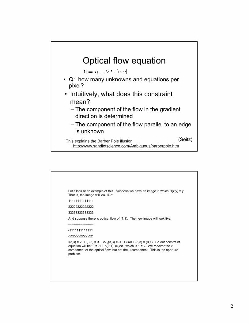
Optical flow equation
• Q: how many unknowns and equations per pixel?
• Intuitively, what does this constraint
mean?– The component of the flow in the gradient
direction is determined
– The component of the flow parallel to an edge
is unknown
This explains the Barber Pole illusion
http://www.sandlotscience.com/Ambiguous/barberpole.htm
(Seitz)
Let’s look at an example of this. Suppose we have an image in which H(x,y) = y.
That is, the image will look like:
11111111111111
22222222222222
33333333333333
And suppose there is optical flow of (1,1). The new image will look like:
-----------------------
-1111111111111
-2222222222222
I(3,3) = 2. H(3,3) = 3. So It(3,3) = -1. GRAD I(3,3) = (0,1). So our constraint
equation will be: 0 = -1 + <(0,1), (u,v)>, which is 1 = v. We recover the v
component of the optical flow, but not the u component. This is the aperture
problem.
3
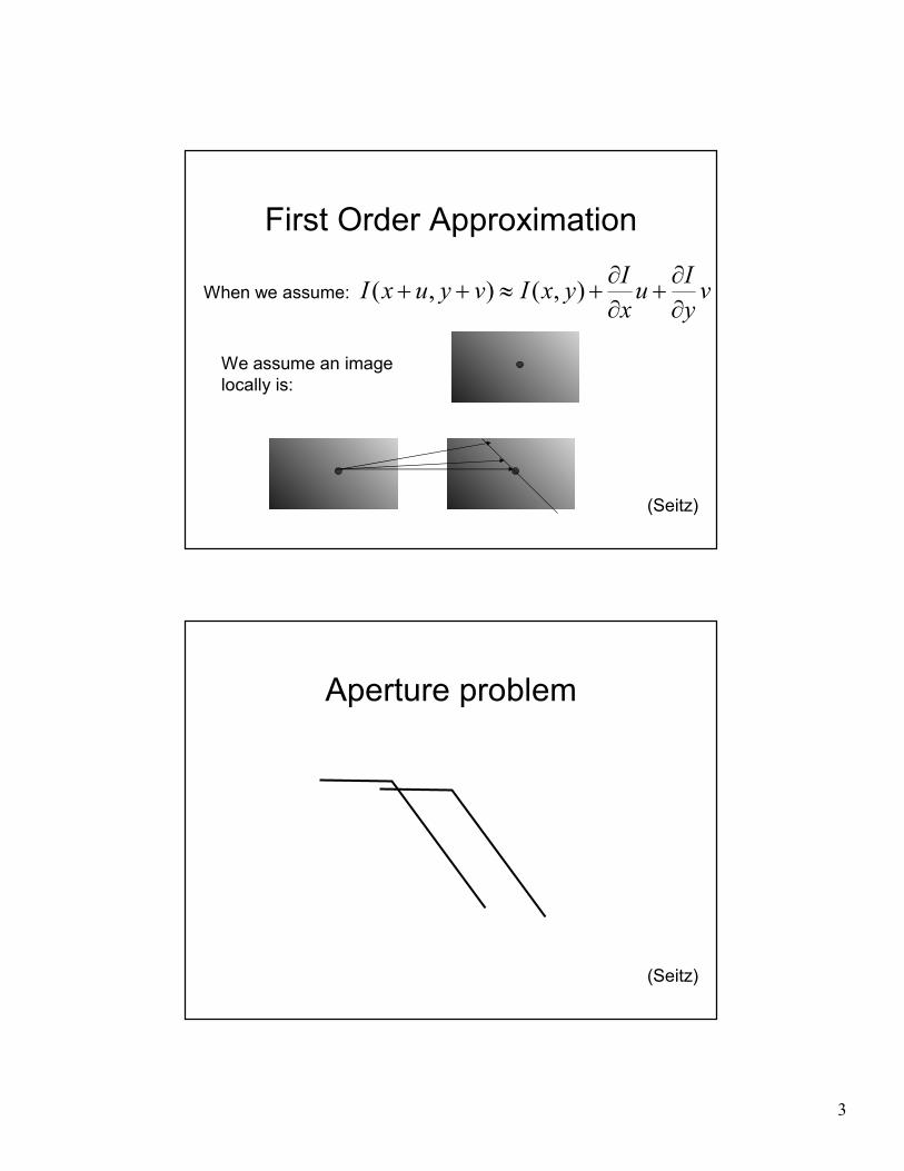
First Order Approximation
When we assume:
We assume an image
locally is:
(Seitz)
vy
Iux
IyxIvyuxI
∂
∂+
∂
∂+≈++ ),(),(
Aperture problem
(Seitz)

4
Aperture problem
(Seitz)
Solving the aperture problem• How to get more equations for a pixel?
– Basic idea: impose additional constraints
• most common is to assume that the flow field is smooth
locally
• one method: pretend the pixel’s neighbors have the
same (u,v)
– If we use a 5x5 window, that gives us 25 equations per
pixel!
(Seitz)

5
Lukas-Kanade flow
• We have more equations than unknowns: solve least squares problem. This is given by:
– Summations over all pixels in the KxK window
– Does look familiar? (Seitz)
Let’s look at an example of this. Suppose we have an image with a corner.
1111111111 -----------------
1222222222 And this translates down and to the right: -1111111111
1233333333 -1222222222
1234444444 -1233333333
Let’s compute It for the whole second image:
---------- Ix = ---------- Iy = -------------
0-1-1-1-1-1 --00000 --------------
-1-1-1-1-1-1 --.50000 -0-.5-1-1-1-1-1-1
-1-1-1-1-1-1- --1.5000 -00-.5-1-1-1-1-1
Then the equations we get have the form:
(.5,-.5)*(u,v) = 1, (1,0)*(u,v) = 1, (0,-1)(u,v) = 1.
Together, these lead to a solution that u = 1, v = -1.

6
Conditions for solvability
– Optimal (u, v) satisfies Lucas-Kanade equation
When is This Solvable?• ATA should be invertible
• ATA should not be too small due to noise
– eigenvalues λ1 and λ2 of ATA should not be too small
• ATA should be well-conditioned
– λ1/ λ2 should not be too large (λ1 = larger eigenvalue) (Seitz)
Does this seem familiar?
Formula for Finding Corners
=
∑∑∑∑
2
2
yyx
yxx
III
IIIC
We look at matrix:
Sum over a small region,
the hypothetical corner
Gradient with respect to x,
times gradient with respect to y
Matrix is symmetric WHY THIS?

7
=
=
∑∑∑∑
2
1
2
2
0
0
λ
λ
yyx
yxx
III
IIIC
First, consider case where:
This means all gradients in neighborhood are:
(k,0) or (0, c) or (0, 0) (or off-diagonals cancel).
What is region like if:
1. λ1 = 0?
2. λ2 = 0?
3. λ1 = 0 and λ2 = 0?
4. λ1 > 0 and λ2 > 0?
General Case:
From Singular Value Decomposition it follows
that since C is symmetric:
RRC
= −
2
11
0
0
λ
λ
where R is a rotation matrix.
So every case is like one on last slide.

8
So, corners are the things we
can track
• Corners are when λ1, λ2 are big; this is also when Lucas-Kanade works.
• Corners are regions with two different
directions of gradient (at least).
• Aperture problem disappears at
corners.
• At corners, 1st order approximation fails.
Edge
– large gradients, all the same
– large λ1, small λ2(Seitz)

9
Low texture region
– gradients have small magnitude
– small λ1, small λ2(Seitz)
High textured region
– gradients are different, large magnitudes
– large λ1, large λ2(Seitz)

10
Observation
• This is a two image problem BUT– Can measure sensitivity by just looking at one of
the images!
– This tells us which pixels are easy to track, which
are hard
• very useful later on when we do feature tracking...
(Seitz)
Errors in Lukas-Kanade
• What are the potential causes of errors in this procedure?– Suppose ATA is easily invertible
– Suppose there is not much noise in the image
• When our assumptions are violated
– Brightness constancy is not satisfied
– The motion is not small
– A point does not move like its neighbors
• window size is too large
• what is the ideal window size? (Seitz)

11
Iterative Refinement
• Iterative Lukas-Kanade Algorithm1. Estimate velocity at each pixel by solving Lucas-
Kanade equations
2. Warp H towards I using the estimated flow field
- use bilinear interpolation
- Repeat until convergence
(Seitz)
If Motion Larger: Reduce the
resolution (Seitz)

12
Optical flow result
Dewey morph (Seitz)
Tracking features over many
Frames
• Compute optical flow for that feature for each consecutive H, I
• When will this go wrong?
– Occlusions—feature may disappear
• need to delete, add new features
– Changes in shape, orientation
• allow the feature to deform
– Changes in color
– Large motions
• will pyramid techniques work for feature
tracking?
(Seitz)

13
Applications:
• MPEG—application of feature tracking
– http://www.pixeltools.com/pixweb2.html
(Seitz)
Image alignment
• Goal: estimate single (u,v) translation for entire image
– Easier subcase: solvable by pyramid-based Lukas-Kanade
(Seitz)

14
Summary
• Matching: find translation of region to minimize SSD.– Works well for small motion.
– Works pretty well for recognition sometimes.
• Need good algorithms.– Brute force.
– Lucas-Kanade for small motion.
– Multiscale.
• Aperture problem: solve using corners.– Other solutions use normal flow.