Selected Ideas in the MathematicalCareer of F. S. Cater

Dedicated toPaul White

Whose teaching inspired myinterest in real variables

Preface

This pamphlet contains a collection of selected ideas from the mathematicalcareer of F. S. Cater. In each case we give a reference of a paper or part of apaper. However, on occasion we do not have a reference so we write a shortnote (paper) in this pamphlet.

One purpose of the pamphlet is to gather these ideas together so we donot have to hunt them down in the literature. We can see the picture as awhole and identify quickly what we want to read. The best place to read thepamphlet is in a library where the Real Analysis Exchange and certain otherjournals are on the shelf, or by a computer that serves the same purpose.

Most of my career, and these ideas, are in real variables (real analysis)though there are occasional forays into linear algebra and topology (consultthe short Chapter IV, for example).

The Chapters gather ideas that are most connected. In Chapter I weconsider derivatives and differentiation, and nowhere differentiable functions.In Chapter II we consider families of continuous functions. For example, thismay include C(X) or some subfamily of C(X) for a topological space X —in particular when X is a subset of R. In Chapter III we consider absolutelycontinuous functions and N-functions (f is an N-function if f maps sets ofmeasure zero to sets of measure zero). Chapter IV is a short chapter (4items) on the algebra of matrices. We have real variables again when theentries in the matrices are real numbers. In Chapter V we have alternativearguments. These are essentially different from the arguments they replace.For example, the alternative argument may be much simpler, or much shorterthan the conventional argument. Another possibility is that the alternativeargument requires much less sophisticated background than the conventionalargument. Finally, Chapter VI is called Variety. It consists chiefly of ideasthat we did not see fit to insert in other Chapters. In the first item of ChapterVI we find that my Erdos number is one.

i

Some items could possibly be in more than one Chapter. Many ideas inmy papers were not included because I wanted to reduce the length. Thentoo, after many years there is much that may have interested me at onetime, but no longer does. Sorry if I deleted your favorite topic in my papers.Finally, I selected items with the pamphlet as a whole in mind.

F. S. CaterPortland, Oregon

August, 2009.

ii

Contents

Preface i

I Derivatives and Differentiation 2I.1 A typical nowhere differentiable function . . . . . . . . . . . 2I.2 Nondifferentiability of a certain sum . . . . . . . . . . . . . . 3I.3 A derivative often zero and discontinuous . . . . . . . . . . . 3I.4 An increasing continuous function with Dini derivates 0

and ∞ . . . . . . . . . . . . . . . . . . . . . . . . . . . . . . 3I.5 Constructing nondifferentiable functions from concave func-

tions . . . . . . . . . . . . . . . . . . . . . . . . . . . . . . . 4I.6 Sums of jump functions . . . . . . . . . . . . . . . . . . . . . 4I.7 On the range of a real function . . . . . . . . . . . . . . . . 5I.8 Using derivates to partition R . . . . . . . . . . . . . . . . . 5

II Families of continuous functions 8II.1 Function lattices. . . . . . . . . . . . . . . . . . . . . . . . . 8II.2 Nonlinear mappings . . . . . . . . . . . . . . . . . . . . . . . 8II.3 Function rings . . . . . . . . . . . . . . . . . . . . . . . . . . 9II.4 Spaces of functions . . . . . . . . . . . . . . . . . . . . . . . 9II.5 Lattice automorphisms . . . . . . . . . . . . . . . . . . . . . 10II.6 Functions with frequently infinite derivatives . . . . . . . . . 10II.7 On derivatives of functions of bounded variation . . . . . . . 11

IIIAbsolute continuity and the Lusin Property (N) 13III.1 An equation for absolute continuity . . . . . . . . . . . . . . 13III.2 Summable and absolutely continuous functions . . . . . . . . 14III.3 Knot points and N -functions . . . . . . . . . . . . . . . . . . 14III.4 Completing an N -function example . . . . . . . . . . . . . . 15

iii

III.5 Compact sets and N -functions . . . . . . . . . . . . . . . . . 15III.6 N -functions relative to a closed set . . . . . . . . . . . . . . 15

IV Matrix algebra 17IV.1 The matrix factor theorem . . . . . . . . . . . . . . . . . . . 17IV.2 Determinants and scalar mappings . . . . . . . . . . . . . . 20IV.3 On multiplicative mappings . . . . . . . . . . . . . . . . . . 20IV.4 Text Book . . . . . . . . . . . . . . . . . . . . . . . . . . . . 21

V Alternative arguments 22V.1 On infinite unilateral derivatives . . . . . . . . . . . . . . . . 22V.2 A theorem of de la Vallee Poussin . . . . . . . . . . . . . . . 22V.3 Geodesics on spheres in Hilbert space . . . . . . . . . . . . . 23V.4 Open mappings . . . . . . . . . . . . . . . . . . . . . . . . . 23V.5 On finitely generated abelian groups . . . . . . . . . . . . . 24V.6 Salad Days . . . . . . . . . . . . . . . . . . . . . . . . . . . 26V.7 On Lp-spaces where 0 < p < 1 . . . . . . . . . . . . . . . . . 26V.8 On sets where unilateral derivatives are infinite . . . . . . . 27

VI Variety 30VI.1 Foray into point-set topology . . . . . . . . . . . . . . . . . 30VI.2 Certain nonconvex linear topological spaces . . . . . . . . . 31VI.3 Linear functionals on certain linear topological spaces . . . . 31VI.4 Foray into fields . . . . . . . . . . . . . . . . . . . . . . . . . 31VI.5 Collectionwise normal spaces . . . . . . . . . . . . . . . . . . 32VI.6 On real functions of two variables . . . . . . . . . . . . . . . 32VI.7 A variation on T1-functions . . . . . . . . . . . . . . . . . . 33VI.8 Functions having equal ranges . . . . . . . . . . . . . . . . . 33VI.9 Foray into ring theory . . . . . . . . . . . . . . . . . . . . . 34VI.10 Mappings into sets of measure zero . . . . . . . . . . . . . . 34VI.11 On upper and lower integrals . . . . . . . . . . . . . . . . . 35VI.12 On closed subsets of uncountable closed sets . . . . . . . . . 35

Postscript 38

1

Chapter I

Derivatives and Differentiation

I.1 A typical nowhere differentiable function

After much experimenting over a period of years, we discovered that thecontinuous real valued function

F (x) =∞∑n=1

2−n! cos(2(2n)!x)

satisfies the properties:

(i) At each x either D+F (x) = −D−F (x) =∞ or D−F (x) = −D+F (x) =∞, and the set of x where either equation does not hold is a firstcategory set of measure zero,

(ii) At each x, [D−F (x), D−F (x)] ∪ [D+F (x), D+F (x)] = [−∞,∞],

(iii) Each of the four sets {x : F ′+(x) = ∞}, {x : F ′+(x) = −∞}, {x :F ′−(x) = ∞}, {x : F ′−(x) = −∞} contains a perfect set in every inter-val, and hence has the power of the continuum in every interval.

It is known that in the metric space of continuous functions on [0, 1] underthe uniform norm, functions satisfying (i), (ii) and (iii) form a residual set.However it is difficult to find a succinct definition of such a function, likeours. Our paper is F.S. Cater “A typical nowhere differentiable function,”Canadian Math. Bull. 26(2), 1983, 149-151.

To read more about functions satisfying (i), (ii) and (iii) consult, for ex-ample, K.M. Garg “On a residual set of continuous functions,” CzechoslovakMath. Journal 20 (1970), 537-543.

2

I.2 Nondifferentiability of a certain sum

Let b > 1 (b is not necessarily an integer) and let cn be any real number foreach index n. Let K(x) denote the distance from x to the nearest integer.In connection with their own work in the 1990s, A. Baouche and S. Dubucinquired about the differential status of the function

F (x) =∞∑n=0

K(bnx+ cn)/bn, (b > 1).

In F.S. Cater, “Remark on a function without unilateral derivatives,”Journal of Math. Analysis and Applications 182 (3), March 1994, 718-721,we gave a partial answer.

We proved that F has no finite unilateral derivative at any point if b ≥ 10.At this writing, I do not know what the status of F is for 1 < b < 10.

I.3 A derivative often zero and discontinuous

We give a constructive definition of a derivative h on [0, 1] that is discontin-uous almost everywhere on [0, 1] but vanishes on a set of positive measure ineach subinterval of [0, 1]. Our paper is F.S. Cater “A derivative often zeroand discontinuous,” Real Analysis Exchange 11, (1985-86), 265-270.

It was written in reply to Clifford Weil “The space of bounded deriva-tives,” Real Analysis Exchange 3, (1977-78), 38-41, where a category argu-ment was used to prove the existence of a derivative on [0, 1] that vanisheson a dense subset of [0, 1] but is nonzero almost everywhere.

I.4 An increasing continuous function with

Dini derivates 0 and ∞In F.S. Cater “On the Dini derivates of a particular function,” Real AnalysisExchange 25 (1), 1999-2000, 1-4, we constructed a continuous strictly increas-ing function f such that at each point x, either D+f(x) = 0 or D+f(x) =∞,and at each point x, either D−f(x) = 0 or D−f(x) =∞. Moreover, 0 or ∞is a derivate (left or right) at each point.

3

I.5 Constructing nondifferentiable functions

from concave functions

Let (an) be a sequence of nonnegative real numbers such that∑∞

n an <∞.Let (bn) be a strictly increasing sequence of positive numbers such that bndivides bn+1 for each n, and (anbn) does not converge to zero.

Let f be a continuous function mapping the real line onto the interval[0, 1] such that f(1) = 1, f(0) = f(2) = 0, and f is concave down on theinterval [0, 2]. Let f(x+ 2) = f(x) for each x.

In F.S. Cater, “Constructing nowhere differentiable functions from convexfunctions,” Real Analysis Exchange 28 (2), 2002-2003, 617-622, we provedthat

∞∑j=1

ajf(bjx)

has a finite left or right derivative at no point.In this way, we can construct nowhere differentiable functions out of con-

cave (and convex functions. Several examples were offered.Later it was pointed out to me that I had inadvertently interchanged

the definitions of “convex” and “concave”in the paper. Sorry about that. Ialways thought that a bump in the road

��was convex, but a pot

hole in the road � was concave. No matter.

I.6 Sums of jump functions

By a jump function centered at a point x in R we mean a real functions onR, constant on the intervals (−∞, x) and (x,∞) such that

f(x−) ≤ f(x) ≤ f(x+) and f(x−) < f(x+).

In G. Piranian “The derivative of a monotone discontinuous function,”Proc. of the Amer. Math. Soc, 16(2), 1965, 243-244, George Piranian provedthat if S is a countable Gδ-set in R, then there exists a nondecreasing functionf on R with infinite derivative at each point in S and zero derivative at eachpoint not in S. He made f the sum of jump functions centered at the pointsin S. Thus f was also discontinuous at each point of S in his construction.

In F.S. Cater “On functions differentiable on complements of countablesets,” Real Analysis Exchange, 32(2), 2006-2007, 527-536, we proved that if g

4

is a nondecreasing bounded function with zero derivative at all but countablemany points, and g has infinite derivative at every other point, then g canbe expressed as the sum of (countably many) jump functions. Furthermore,the set of all points where g has infinite derivative is necessarily a nowheredense Gδ-set.

For example, there exists no nondecreasing function g, discontinuous atevery rational point, that has zero derivative at every irrational point.

I.7 On the range of a real function

Let f be a real function on R, and let {Iv} denote a family of intervalscovering a set S such that m(S ∩ Iv) ≤ m(f(S ∩ Iv)) for each Iv. (Here mdenotes Lebesgue outer measure.) In F.S. Cater, “Note on the outer measuresof images of sets,” Real Analysis Exchange, 26(2), 2000-2001, 827-830, weproved that m(f(S)) ≤ 2m(S). We showed by example that no coefficientless than 2 will suffice here in general.

Observe that this does not necessarily involve derivatives.

I.8 Using derivates to partition R

In this item we use derivates of a function to give a constructive definitionof a partition of R into continuum many Fσδ-sets, each of which meets everysubinterval of R in continuum many points. We do not have a paper onthis construction so we write it here. We do not use or need the ContinuumHypothesis.

Let f be a continuous nondecreasing functions from [0, 1] onto [0, 1] thathas zero derivative almost everywhere. For each n positive, negative or zeroand x ∈ [0, 1], put

f0(n+ x) = n+ f(x).

Then f0 is a continuous nondecreasing function from R onto R with zeroderivative almost everywhere. Put

H(x) =∞∑n=0

2−nf0(nx).

5

By the “other” Fubini Theorem (consult (17.18) of Hewitt & Stromberg,Real and Abstract Analysis, Springer, New York, 1965), H ′ = 0 almost ev-erywhere. Moreover H is strictly increasing on R.

For each extended real number r, 0 ≤ r ≤ ∞, put

Tr = {x : D+H(x) = r}.

The Tr apparently form a partition of R composed of continuum manysets. It remains to prove that the desired hypotheses are satisfied.

Lemma 1. For each extended real number r, 0 < r <∞, Tr meets everyinterval in continuum many points.

Proof. The complement of T0 has measure zero, so the set

H{x : 0 < D+H(x) <∞}

has measure zero. Because D+H vanishes on T0 it follows that the set

H{x : D+H(x) = 0}

also has measure zero. We deduce that for any interval I,

H{x ∈ I : D+H(x) =∞}

has positive measure. It follows that I ∩T∞ has the power of the continuum.But the complement of T0 has measure zero, so I ∩ T0 also has the power ofthe continuum.

So now let r be a real number 0 < r < ∞, and let I be any interval.Let g be a continuous function on R such that g(x) = H(x) for x ∈ I, andg′(x) > r for x outside the closure of I.

It follows that D+g > r on a dense subset of R. There is evidently apoint x0 ∈ I where

D+g(x0) = D+H(x0) = 0 < r

because T0 is dense in R. It follows from Anthony Morse “Dini derivates ofa continuous function”, Proc. Amer. Math. Soc, 5 (1954), 126-130, that{x : D+g(x) = r} has continuum many points. It follows that

I ∩ Tr = {x ∈ I : D+H(x) = r}

has continuum many points.

6

To complete the argument, we need one more well-known Lemma. Weinclude a proof of it for any one who wants one written here.

Lemma 2. For each extended real number r, 0 < r <∞, the set Tr is anFσδ-subset of R.

Proof. Let r be a positive real number and let n be a positive integer.Then it follows that the set

Sn = {x : there exists a y > x such that (H(y)−H(x)) > r(y−x), 0 < y−x < n−1}

is open. Then the set Pr = ∩∞n=1Sn is a Gδ-set. Clearly Pr contains the set{x : D+H(x) > r} and Pr is disjoint from the set {x : D+H(x) < r}. Itfollows that

T∞ =∞⋂k=1

Pk

is a Gδ-set and consequently T∞ is also an Fσδ-set. Furthermore

Tr =

[∞⋂k=1

Pr−k−1

]\

[∞⋃k=1

Pr+k−1

]

is a Gδ-set minus a Gδσ-set, and in turn is the intersection of a Gδ-set withan Fσδ-set. Finally, Tr is the intersection of two Fσδ-sets and is an Fσδ-set.

Observe that the function f completely determines the partition in thisargument. Consequently, when f is Lebesgue’s singular function, the def-inition of f is constructive and the definition of the partition is likewiseconstructive.

You also may be interested in the paper Amer. Math. Monthly 91 (9),November 1984, 564-566, in which we partitioned (0, 1) into countably manymeasurable sets that each meet every subinterval of (0, 1) in a second categoryset of positive measure. However, we cannot make these measurable sets allBorel sets.

7

Chapter II

Families of continuous functions

II.1 Function lattices.

Let U be a locally compact Hausdorff space that is not compact. Let L(U)denote the family of all continuous real valued functions f on U such that forsome nonzero number p, depending on f , f−p vanishes at infinity. Now let Sbe a locally compact Hausdorff space. Define T (S) to be C(S) if S is compact,and define T (S) to be L(S) if S is not compact. In F.S. Cater “Some latticesof continuous functions on locally compact spaces”, Real Analysis Exchange33(2), 2007-2008, 285-290, we proved that for any locally compact spaces S1

and S2, S1 and S2 are homeomorphic spaces if and only if T (S1) and T (S2)are isomorphic lattices.

Thus T (S) assumes a similar role for locally compact spaces S that C(X)assumes for compact spaces X.

II.2 Nonlinear mappings

Let X be a compact Hausdorff space, and let D(X) denote the family of allcontinuous functions f on X satisfying 0 ≤ f ≤ 1. In S. Cater “A nonlineargeneralization of a theorem on function algebras,” Amer. Math. Monthly74 (#4), June-July, 1967, 682-685, we proved the following result.

Theorem 1. Let X be a compact Hausdorff space and let u be a mappingof D(X) into the unit interval [0, 1] such that(1) u(fg) = u(f)u(g) for f, g ∈ D(X),(2) u(1− f) = 1− u(f) for f ∈ D(X).

8

Then there is a unique point x0 ∈ X such that u(f) = f(x0) for allf ∈ D(X).

This result will be used in the next Item.(Note: At that time I was known as S. Cater, an exaggerated attempt at

brevity on my part. Now there exists another S. Cater, about whom I knownothing.)

II.3 Function rings

For a compact Hausdorffspace X let C(X) denote the ring of continuous func-tions on X. For a locally compact, noncompact space Y let G(Y ) denote thering of continuous functions f on Y such that there exists an integer p, de-pending on f , for which f−p vanishes at infinity on Y . For a locally compactspace W , let P (W ) = C(W ) if W is compact, and let P (W ) = G(W ) if Wis not compact. In Frank S. Cater “Variations on a theorem on rings of con-tinuous functions,” Real Analysis Exchange 24 (2), 1998-1999, 579-588, weproved that locally compact spaces W1 and W2 are homeomorphic spaces ifand only if P (W1) and P (W2) are isomorphic rings.

Thus the ring P (W ) plays a similar role for locally compact W that thering C(X) plays for compact X.

Finally, for real numbers a and b put a ∗ b = ab − a. All this works justas well when the ring isomorphisms are replaced by bijections φ preservingthe one operation ∗:

φ(f(x) ∗ g(x)) = φ(f(x)) ∗ φ(g(x)).

One typo: on page 583, “homomorphism” should be “homeomorphism.”(This time they called me “Frank S. Cater” which is the name I use in

business.)

II.4 Spaces of functions

In F.S.Cater “On sparse subspaces of C[0, 1],” Real Analysis Exchange 31(1), 2005-2006, 7-12, we proved that there exists a subspace H of C[0, 1]under the uniform metric that is homeomorphic to the full space C[0, 1],even though H consists only of infinitely many times differentiable membersof C[0, 1]. Likewise, there is a subspace H1 of C[0, 1], composed only of

9

singular functions of bounded variation, such that H1 is homeomorphic toC[0, 1]. Furthermore, there exists a subspace H2 of C[0, 1], composed only ofnowhere differentiable functions, such that H2 is homeomorphic to C[0, 1].

II.5 Lattice automorphisms

Let φ be a lattice automorphism of the lattice C(X) where X is a compactHausdorff space. Thus for f , g ∈ C(X), f−g ≥ 0 if and only if φ(f)−φ(g) ≥0. We say that φ is increasing provided for f , g ∈ C(X), f−g never vanisheson X if and only if φ(f) − φ(g) never vanishes on X. There are compactHausdorff spacesX that admit lattice automorphisms that are not increasing.One such space is the Stone-Cech compactification of the real line.

In Theorem IV of F.S. Cater “Remark on a result of Kaplansky concern-ing C(X),” Michigan Math. Journal12(1965),97-103, we proved thatevery lattice automorphism must be increasing provided X is either locallyconnected or sequentially compact. I was surprised by the role of “locallyconnected” but I was not surprised by the role of “sequentially compact.”

We deduce that the Stone-Cech compactification of the real line is con-nected but not locally connected.

(Note: After publication it was pointed out to me that there was a prob-lem with Theorem II and its proof in the paper cited above. In retrospect,I should have written a short note on Theorem IV instead of the Michiganpaper. Sorry. Theorem IV and its proof depend in no way on Theorem II.)

II.6 Functions with frequently infinite deriva-

tives

In F.S. Cater, “On infinite unilateral derivatives,” Real Analysis Exchange33(2), 2007-2008, 309-316, we proved that for any continuous function f on[a, b], there exists a continuous function K on [a, b] such that K − f has zeroderivative almost everywhere, and every subinterval I contains continuummany points where K ′+ = ∞, continuum many points where K ′− = ∞,continuum many points where K ′+ = −∞, and continuum many points whereK ′− = −∞. Note that K and f have the same Dini derivates at almost everypoint. For certain functions f , for example, N -functions and functions of

10

bounded variation, K can be selected so that the infinite derivatives arebilateral.

For more about N -functions, consult Chapter III.

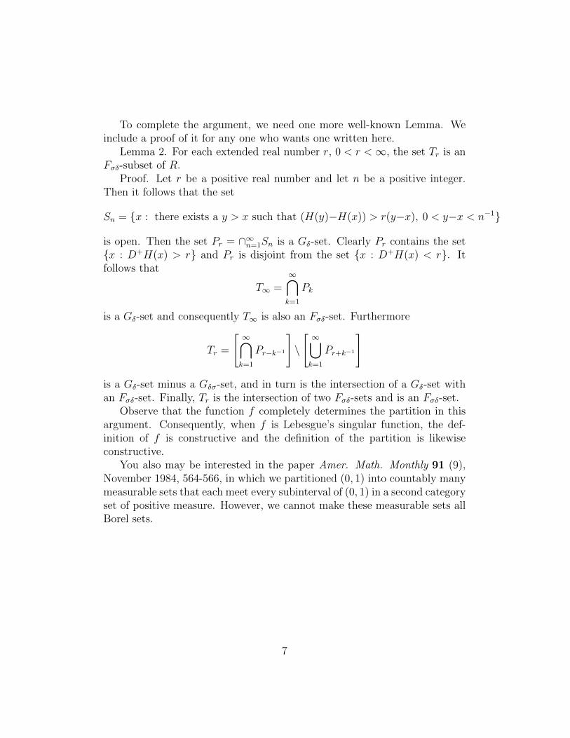
II.7 On derivatives of functions of bounded

variation

This Item is a supplement to our paper F.S. Cater “On the derivatives offunctions of bounded variation,” Real Analysis Exchange 26(2), 2000-2001,923-932.

Let F denote the family of all continuous functions of bounded variationon the interval [0, 1]. The uniform metric is not complete on F . A betterchoice is the complete metric w for which

w(f, g) = |f(0)− g(0)|+ total variation of f − g on [0, 1].

We say that something is true of a “typical” function in F if the set ofall functions in F for which it is not true is a first category subset of F .

For consistency, theorem III in our paper should read:“The restriction of the derivative of a typical function f to its set of points ofdifferentiability is unbounded in every subinterval”. Indeed we proved thatfor typical functions f , the range of f ′ on any subinterval is dense in R.

To show that the absolute value bars can be removed in theorem I of ourpaper, argue as follows.

Proof. Let f ∈ F, ε > 0, and let (a, b) be any subinterval of [0, 1].We use Lemma 2 of our paper F.S. Cater “On infinite unilateral deriva-

tives”, Real Analysis Exchange 33(2), 2007/2008, pp. 309-216, to constructa continuous nondecreasing singular function g ∈ F of total variation 2ε,and vanishing at 0, such that for any h ∈ F with total variation less thanε, (g+ h)′(x) =∞ at continuum many points x of (a, b) at which f is differ-entiable. Then (f, g + h)′(x) = ∞ at all such points x. Let Ka,b denote thefamily of all functions k ∈ F for which k′ =∞ at continuum many points in(a, b). It follows that f +g is an interior point of Ka,b. Now w(f +g, f) = 2ε,so Ka,b contains an open dense subset of F because ε and f were arbitrary.

Let a, b run over the rational numbers in (0, 1). Then

K =⋂

a,b Ka,b

11

has a first category complement in F . But any p ∈ K satisfies p′ = ∞ atcontinuum many points in any subinterval of [0, 1]. The corresponding resultholds for −∞.

We continue as follows. Fix an index n > 0, and typical f ∈ F . Forany x satisfying f ′(x) = ∞ select an interval (c, d) such that f(d) − f(c) >d−c, x ∈ (c, d) and d−c < n−1. Let Sn denote the union of all such intervalsas x runs over all points where f ′ =∞ and n > 0. Let Tn be defined in thesame way where f(d)− f(c) < −(d− c) and f ′(x) = −∞. It follows that⋂

n(Sn ∩ Tn)

is a residual subset of [0, 1] and f can have no derivative, finite or infinite,at any point of this set. Finally, a residual subset of [0, 1] must meet eachsubinterval of [0, 1] in continuum many points.

We recapitulate:For a typical function f in F and any subinterval I of [0, 1], f ′ = ∞ atcontinuum many points of I, f ′ = −∞ at continuum many points of I, andthere are continuum many points of I where f has no derivative, finite orinfinite. Of course every f ∈ F is differentiable almost everywhere.

In the proof of theorem I in our paper we seemed to need the ContinuumHypothesis. It is not needed here.

You also might be interested in our paper “Most monotone functions arenot singular,” �American Math. Monthly 89(7), August-September, 1982, pp.466-469.

12

Chapter III

Absolute continuity and theLusin Property (N)

III.1 An equation for absolute continuity

Let f be a continuous function of bounded variation on [a, b] and let L denotethe length of f [a, b]. For each x ∈ [a, b] let k(x) = 0 if the set

{t ∈ [a, b] : f(t) = f(x)}

is infinite, and k(x) = 1/N if this set has N elements.In Theorem 16 of F.S. Cater “On change of variables in integration,”

Eotvos (vols. XXII-XXIII), 1979-1980, 11-22, we proved that f is absolutelycontinuous on [a, b] if and only if∫ b

a

k(x)|f ′(x)|dx = L.

Thus we express the absolute continuity of a continuous function f ofbounded variation in terms of an equation involving f ′.

A better known necessary and sufficient condition is that f be an N -function on [a, b], that is, f , maps sets of measure zero to sets of measurezero. This is called the Banach-Zarecki Theorem.

13

III.2 Summable and absolutely continuous func-

tions

The Banach-Zarecki Theorem states that a necessary and sufficient conditionfor a continuous function f of bounded variation to be absolutely continuouson an interval is that f be an N -function on that interval.

In F.S. Cater “Some variations on the Banach-Zarecki Theorem,” RealAnalysis Exchange, 32(2),547-552, we proved:

Corollary 1. Let f be a continuous N -function differentiable almost every-where on [a, b]. Then f is absolutely continuous on [a, b] if and only if thereexists a summable function g on [a, b] such that g ≥ f ′ almost everywhereon [a, b].

Corollary 1 is a tolerable variation of (6.9), Chapter IX in S. Saks, Theoryof the Integral, Second revised edition, Dover, New York, 1964. We hope itis of use and of interest in University teaching.

III.3 Knot points and N-functions

By a knot point p of a function f , we mean a point p at which the two upperDini derivates of f are ∞, and the two lower Dini derivates of f are −∞. InF.S. Cater “On continuous N -functions and an example of Mazurkiewicz”,Real Analysis Exchange, 30(1), 2004-2005, 201-206, we proved:

Corollary 3. Let f be a continuous function that is not an N -functionon [a, b], let K be the set of all knot points of f , and let f(K) have measurezero. Then for any everywhere differentiable function g on [a, b], f + g is notan N -function on [a, b].

As an example, let F be a monotone nonconstant continuous function on[0, 1] with F ′ = 0 almost everywhere. Then for any everywhere differentiablefunction g on [0, 1], F + g is not an N=function on [0, 1].

Mazurkiewicz constructed a continuous function M(x) such that M(x)+xis an N -function but M(x) is not. Then M(K) does not have measure zero.

For more about knot points, consult the work of K.M. Garg.In this item we discussed a nexus between knot points and Masurkiewicz-

type functions.

14

III.4 Completing an N-function example

In the Real Analysis Exchange, Summer Symposium 2002, p. 411, we posedthe following research question.

Question. Given a nonconstant continuous N -function f , is there a con-tinuous N -function g, depending on f , such that the sum f + g is not anN -function.

The question was answered in the affirmative in Dusan Pokorny “OnLusin’s (N)-property of the sum of two functions,” Real Analysis Exchange,33(1), 2007-2008, 23-28.

So Pokorny’s Theorem generalizes the Masurkiewicz example from linearfunctions to continuous functions.

We had a hand in this because we posed the research problem in print.

III.5 Compact sets and N-functions

Put f(x) = x in Lemma 1 of F.S. Cater “On continuous N -functions andan example of Mazurkiewicz,” Real Analysis Exchange, 30(1), 2004-2005,201-206, and obtain

Lemma 1. Let h be a continuous function on [a, b] and let S ⊂ [a, b] be aset of measure zero such that h(S) does not have measure zero. Then thereexists a compact subset T of S closure such that T has measure zero buth(T ) has positive measure.

So for a continuous function h to be an N -function it suffices that h mapscompact sets of measure zero to sets of measure zero.

We will use this Lemma in the next Item.

III.6 N-functions relative to a closed set

Say that a function f is an N -function relative to the set P if f maps anysubset of P of measure zero to a set of measure zero.

Here we pose the following question: For any uncountable closed set P ofmeasure zero, do there exist continuous functions F and G on R, dependingon P , that are N -functions relative to R such that the sum F +G is not anN -function relative to P? We will answer this in the affirmative. But we didnot publish it elsewhere, so we write it here.

15

We start with two continuous N -functions f and g with respect to Rsuch that f + g is not an N -function with respect to R. It follows from ItemIII(5) that there is an uncountable compact set X of measure zero such that(f + g)(X) has positive measure. It follows that there is a perfect subsetX1 of X such that X\X1 is at most a countable set. Thus (f + g)(X1) haspositive measure.

Now P has a closed bounded subset P0 that is also uncountable. Thereis a compact perfect subset P1 of P0 such that P0\P1 is at most a countableset. Between any two complementary intervals of P1 there are other comple-mentary intervals of P1. Likewise, between any two complementary intervalsof X1 there are other complementary intervals of X1.

It follows that there is an order preserving bijection K of the set of allcomplementary intervals of P1 onto the set of all complementary intervals ofX1. In an obvious manner K gives rise to an increasing function k of thecomplement of P1 onto the complement of X1 such that k is linear on eachcomponent of the complement of P1.

In the natural way we extend k to an increasing homeomorphism of Ronto R by assigning to each x ∈ P1 the unique point k(x) in X1 that makes keverywhere increasing on R. Note that k then, is an N -function with respectto each component of the complement of P1, and an N -function with respectP1 because X1 has measure zero. It follows that k is an N -functions withrespect to R. Define the composite functions on R

F = f ∗ k, G = g ∗ k.

Now F and G are N -functions with respect to R because f , g and k are.But

F +G = (f + g) ∗ k

maps the set P1 of measure zero to the set (f + g)(X1) that has positivemeasure. It follows that F +G is not an N -function with respect to P1 or P .

REMARK. It can be shown (Item VI(12)) that any closed uncountableset contains an uncountable closed subset of measure zero. Thus it sufficesin our argument that P be any uncountable closed set. I do not know what,if anything, can be concluded if P is only an uncountable set.

16

Chapter IV

Matrix algebra

All matrices are square, n by n, and the entries are in a commutative field,F .

IV.1 The matrix factor theorem

In Lemma 8 of F.S. Cater ”Products of central collineations,” Linear algebraand its applications 19 (1978), 251-274, we have a result I call the Matrixfactor theorem. It can be described as follows:

Let M be a nonsingular n by n nonscalar matrix (not the product ofa scalar with the identity matrix I). Let x1, x2, ...xn be scalars such thatx1x2..., xn = detM . Then there exist matrices M1,M2, ...,Mn such that

(1) the product M1M2...Mn is similar to the matrix M ,(2) detMj = xj for j = 1, 2, ..., n,(3) for each index j = 1, 2, ..., n, all the nonzero entries of Mj − I lie in thej − th column of Mj − I.

The developments of Lemmas 4 and 6 should be clearer so we will giveother proofs here.

Let M be a nonsingular nonscalar matrix. Our arguments will be in asequence of steps.

Step 1. M is similar to a nondiagonal matrix.Proof. Let aij denote the i-th row, j-th column entry of M . Let M be

diagonal. There is an index i with aii 6= a11 because M is not a scalar matrix.Then M is similar to the matrix found by adding the i-th row of M to thefirst row of M , then subtracting the first column from the i-th column. The

17

pattern is suggested by (1 10 1

)M

(1 −10 1

).

Step 2. M is similar to a matrix whose 1-st row is not a scalar multipleof (1, 0, ..., 0).

Proof. In view of Step 1, we assume that M is not a diagonal. Say aij 6= 0where i 6= j. Then M is similar to the matrix found by interchanging thei-th and j-th rows of M , then interchanging the i-th and j-th columns. Theresult is a matrix with an entry equal to the value aij in the first row but notin the first column. The pattern is suggested by(

0 11 0

)M

(0 11 0

).

Step 3. Let p be any nonzero scalar in F . Then M is similar to a matrixwhose first row is (p, p, 0, ..., 0).

Proof. In view of Step 2, we can assume that for some index j > 1,a1j 6= 0. We multiply the first row of M by p/a1j and then multiply the firstcolumn by a1j/p, to find that M is similar to a matrix with p in the first rowand j-th column. The pattern is suggested by(

p/alj 00 1

)M

(alj/p 0

0 1

).

We add (p − a11)/p times the j-th column to the first column and thenadd (a11 − p)/p times the first row to the j-th row to find that M is similarto a matrix with p in the first row first column entry and p in the first rowj-th column entry. If j > 2, we use the same procedure with the secondcolumn in place of the first column to find that M is similar to a matrixwith p in the first row, first and second column entries. We proceed withthe second column in place of the j-th column to convert all the first rowentries after the second to zero. So M is similar to a matrix whose first rowis (p, p, 0, ..., 0). This is essentially Lemma 6 in our paper.

Step 4. Let n = 2. Let x1, x2 ∈ F such that x1x2 = detM . Then M issimilar to a matrix product of the form(

x1 0√1

)(1√

0 x2

).

18

Proof. By Step 6, we can assume that

M =

(x1 x1a b

).

Then

M =

(x1 0a 1

)(1 10 b− a

).

Clearly b− a = x2 because x1x2 = detM . This is essentially Lemma 4 inour paper.

Take Lemmas 5, 7, 8 and 9 as they appear in our paper. Lemma 8, then,is essentially the matrix factor theorem. We used Lemma 9 to give an answerto a question posed by Radjavi.

Here are two typos in our paper. On page 256, the matrix In−1 shouldbe In−2. On page 254, the first matrix appearing after the word “proof” canbe better written. But this is obviated by the arguments here.

Here are some corollaries not included in our paper.Corollary 1. Let A and B be nonsingular, nonscalar matrices that are

not similar, but such that detA = detB. Let |F | > 3. Then A and B canbe factored

A1A2...An = A, B1B2...Bn = B

such that Aj is similar to Bj for j = 1, 2, ..., n.To see this, observe that for u 6= 0, u 6= 1, diagonal (u, 1, ..., 1) is similar

to any matrix C with detC = u provided all the nonzero entries in C − I liein one column.

Corollary 2. Let M be a nonsingular matrix and let c ∈ F such that c 6= 1and cn = detM . Then there exist mutually similar matrices M1,M2, ...,Mn

such that M = M1M2...Mn.We leave the proof.Corollary 3. Let M be a nonsingular matrix and let F be algebraically

closed. Then there is a scalar s such that sM = M1M2...Mn where each Mj2

is the identity matrix.We leave the proof.

19

IV.2 Determinants and scalar mappings

Let p be an mapping from F to F . Let φ be the mapping from the set of nby n matrices into F as follows: For matrix A,

φ(A) = p(detA).

Observe the φ(AB) = φ(BA) because

det(AB) = (detA)(detB) = (detB)(detA) = det(BA).

In S. Cater, “Scalar valued mappings of square matrices,” Amer. Math.Monthly 70(2), 1963, pp. 163-169, we proved that the following are equivalentfor a mapping φ from the set of n by n matrices into F

(1) φ(ABC) = φ(CBA) for any matrices A, B, C,(2) there exists a mapping p from F to F such that for all matrices A,

φ(A) = p(detA).

Moreover, φ is multiplicative if and only if p is multiplicative.This paper was given an honor of sorts. It was reprinted in the Raymond

W. Brink selected mathematical papers, volume 3, Algebra, pp. 321-327,published by the Mathematical Association of America, 1977.

IV.3 On multiplicative mappings

IV(3) was a precursor to IV(2). This time φ1 and φ2 are each multiplicativemappings from the set of n by n matrices to F , the field of complex numbers,that preserves conjugation:

φi(AB) = φi(A)φi(B), φi(A)− = φi(A−),

for all A and B. Let φ1(e1+iI) = φ2(e

1+iI), In S. Cater, “On multiplicativemappings of operators”, Proc. of the Amer. Math. Soc. 13(1), 1962, pp.55-58, we proved that φ1 = φ2 under these hypotheses. Moreover we provedthat φ1(A) = detA if φ1(e

1+iI) = en+ni.

20

IV.4 Text Book

You may be interested in our linear algebra text book Frank S. Cater, Lec-tures on real and complex vector spaces, W. B. Saunders Company, Philadel-phia, 1966.

It went out of print about 1971, but it still can be found in many universitylibraries. It sold few copies – probably fewer than a thousand – but it didreceive good reviews. I wonder if it would have sold better if we had notwritten the functions on the right and the variables on the left. This notationwas all the rage at that time. Note that in the reference in IV(2), the samenotation was used.

Fortunately this notation is not so popular today. My feeling is that itcauses confusion unless it is used in all branches of mathematics, not justlinear algebra. In retrospect, I regret using that notation. I know it causedme confusion in teaching.

21

Chapter V

Alternative arguments

In this chapter we construct proofs of well-known results that are differentfrom the usual proofs given. We try to make our arguments easier (simpler)than the accepted arguments and/or employ more elementary means (firstprinciples). We hope to provide some worthwhile insights into these resultsas well.

V.1 On infinite unilateral derivatives

One result of S. Saks is that in the complete metric space C[0, 1] under thesup norm, the set of functions that have right (left) derivative ∞(−∞) atcontinuum many points in [0,1] form a residual subset of C[0, 1]. Shorterproofs than his had been given, but they required sophisticated results. InF. S. Cater “An elementary proof of a theorem on unilateral derivatives,”Canadian Math. Bull. 29(3), 1986, pp. 341-343, we provided a relativelyshort argument using first principles.

We used the same technique to give a short proof that the functionsin C[0, 1] that have continuum many knot points form a residual subset ofC[0, 1].

V.2 A theorem of de la Vallee Poussin

We give a reasonable short proof from first principles of a classical theoremattributed to de la Vallee Poussin.

22

Theorem. Let f be a real valued function of bounded variation on theinterval [a, b] and let V (x) denote the total variation of f on [a, x]. Let mdenote Lebesgue outer measure. Then there exists a set N ⊂ [a, b] such that

m(V (N)) = m(f(N)) = m(N) = 0

such that for any x ∈ [a, b]\N , f ′(x) and V ′(x) exist, finite or infinite, andfurthermore V ′(x) = |f ′(x)|.

Note that m(N) = 0 is easy to acquire from school analysis, but

m(N) = m(f(N)) = m(V (N)) = 0

is much harder to acquire. Our paper is F. S. Cater “A new elementaryproof of a theorem of de la Vallee Poussin,” Real Analysis Exchange 27(1),2001/2002, pp. 393-396.

We hope our argument will make this classical Theorem more accessiblein the Universities.

V.3 Geodesics on spheres in Hilbert space

Here we make a foray into geometry. Let S be a sphere in a Euclidean spaceof dimension greater then 2, or a real Hilbert space, and let A and B be twopoints on S that are not antipodal. We give an elementary geometry proofthat the shortest path on S joining points A and B lies on the great circlejoining A and B (that is, the intersection of S with the plane through A, Band the center of S.)

We consider all the continuous rectifiable curves on S, continuously dif-ferentiable or not. We do not need geometric curvature of any kind. Ourpaper is:

F. S. Cater “On the curves of minimal length on spheres in real Hilbertspaces,” Real Analysis Exchange 25(2), 1999/2000, pp. 781-786.

This work was done for teacher education people in our Department whowanted a proof in 3-space without the use of curvature.

V.4 Open mappings

We use real variable arguments to prove the theorem in complex variables,that the image of a nowhere constant analytic function on an open region

23

is an open set. Such a function must be an open mapping, that is, mapsopen sets to open sets. Our paper is: F. S. Cater “An elementary proofthat analytic functions are open mappings,” Real Analysis Exchange 27(1),2001/2002, pp. 389-392. (One typo: In the statement of Lemma 1, “. . . f(0)and the set f(B) . . . ” should be “. . . f(0) to the set f(B) . . . ”. My fault –sorry.)

We used our technique to find yet another proof of the fundamental The-orem of Algebra.

Real variable proofs of complex variable theorems are especially difficult.For our purposes we regarded an analytic function to be a function thatcoincides locally with the sum of a power series about each point. For moreabout real analysis proofs of results concerning complex valued functions,consult: F. S. Cater “Another application of Rolle’s theorem,” Real AnalysisExchange 30(2), 2004/2005, pp. 795-798.

V.5 On finitely generated abelian groups

In “Uniqueness of the decomposition of finite abelian groups: a simple proof,”Mathematics Magazine 71(1), February 1998, pp. 50-52, we gave an elemen-tary proof (from first principles) of the uniqueness of the decomposition offinite abelian groups. This can be expressed as follows:

Theorem. Let G be a finite abelian group. Let

G = G1 ⊕G2 ⊕ · · · ⊕Gm = H1 ⊕H2 ⊕ · · · ⊕Hn

be two decompositions of G; that is, all the Gi and Hi are cyclic subgroupsof G, and order Gi divides order Gi+1 for 1 ≤ i ≤ m−1, and order Hi dividesorder Hi+1 for 1 ≤ i ≤ n − 1. Then n = m and order Gi = order H1 for1 ≤ i ≤ n.

The proof usually requires considerable machinery, but we gave a shortproof using only first principles. There was one typo: on the last page, “Case2. Let r < s” . . . should be “Case 2. Let r > s” . . . . My fault–sorry.

ADDENDUM.We prove the followingLemma. Let K be a torsion free abelian group; that is, every nonzero

element in K has infinite order. Let

K = K1 ⊕K2 ⊕ · · · ⊕Kn = H1 ⊕H2 ⊕ · · · ⊕Hm

24

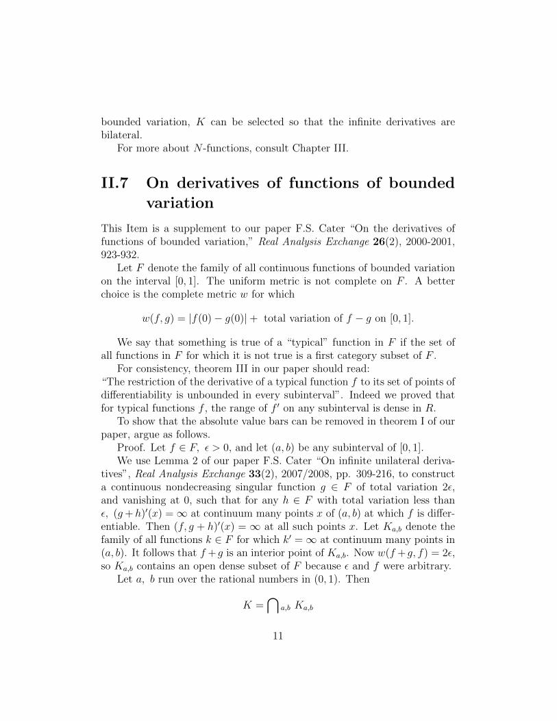
where each Ki and Hi is an infinite cyclic subgroup of K. Then n = m.Proof. We argue by contradiction. Let n < m. We will employ vector

space theory. Let v1, v2, . . . , vn be an ordered basis of an n-dimensional vectorspace V over the field of rational numbers. Let K be the family of vectors(elements) of the form

∑ni=1 aivi where each ai is an integer. Then K is a

subgroup of the additive group of V . Moreover K is the direct sum of ninfinite cyclic groups of the form {avi} for integers a and each i = 1, 2, . . . , n.

By hypothesis, K is also the direct sum ofm infinite cyclic groupsH1, H2, . . . , Hm.For each i = 1, 2, . . . ,m select a nonzero element ui in Hi. Then there existrational numbers b1, b2, . . . , bm, not all zero, such that

m∑i=1

biui = 0 (1)

because m exceeds the dimension of V . Let s be the product of all theinteger denominators of the rational numbers bi. Hence sbi is an integer fori = 1, 2 . . . ,m, not all zero. Add the left side of (1) with itself enough timesto obtain

s

(m∑i=1

biui

)=

m∑i=1

(sbi)ui = 0, (2)

not all sbi = 0. But (sbi)ui ∈ Hi, and it follows that the sum

H1 +H2 + · · ·+Hm

can not be a direct sum. This contradiction proves n ≥ m. The proof ofm ≥ n is analogous.

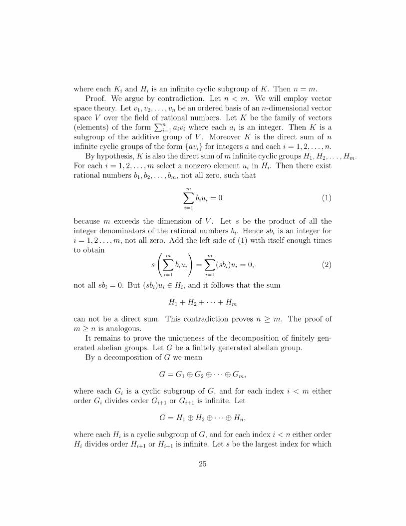
It remains to prove the uniqueness of the decomposition of finitely gen-erated abelian groups. Let G be a finitely generated abelian group.

By a decomposition of G we mean

G = G1 ⊕G2 ⊕ · · · ⊕Gm,

where each Gi is a cyclic subgroup of G, and for each index i < m eitherorder Gi divides order Gi+1 or Gi+1 is infinite. Let

G = H1 ⊕H2 ⊕ · · · ⊕Hn,

where each Hi is a cyclic subgroup of G, and for each index i < n either orderHi divides order Hi+1 or Hi+1 is infinite. Let s be the largest index for which

25

Gs is finite and let t be the largest index for which Ht is finite. Let P denotethe subgroup composed of all the elements of finite order in G. Clearly

P = G1 ⊕G2 ⊕ · · · ⊕Gs = H1 ⊕H2 ⊕ · · · ⊕Ht

and P is a finite group. By the Theorem s = t and order Gi = order Hi fori = 1, 2, . . . , s. For the quotient group G/P it is clear that

G/P = Gs+1 ⊕ · · · ⊕Gm = Ht+1 ⊕ · · · ⊕Hn,

By the Lemma, m− s = n− t. But s = t, and it follows that m = n.We hope these arguments are of some use in University teaching.

V.6 Salad Days

We get a glimpse of me in my salad days in S. Cater “An elementary devel-opment of the Jordan Canonical Form,” Amer. Math. Monthly 69(5), May1962, pp. 391-393.

We gave another argument there in which the underlying field is alge-braically closed and we did not use determinants. At the time (circa 1962) itwould have been very difficult to find a proof without determinants in print.I suppose this state of affairs is different today.

V.7 On Lp-spaces where 0 < p < 1

Let p be a real number, 0 < p < 1, and let Lp denote the family of all

functions f on [0, 1] for which∫ 1

0|f |p < ∞, where two such functions are

regarded as the same if they differ only on a set of measure zero. Put

ζ(f, g) =

∫ 1

0

|f − g|p.

It is shown in M. M. Day “The spaces Lp where 0 < p < 1,” Bull. Amer.Math. Soc. 46 (1940), pp. 816-823, that Lp is a real topological linear spaceunder the metric ζ that has no nonzero continuous linear functional. TheRadon-Nikodym theorem is central to his argument. In S. Cater “Note ona theorem of Day, ” Amer. Math. Monthly 69(7), 1962, pp. 638-640, weprove that there is no nonzero continuous linear functional on Lp using firstprinciples without the Radon-Wikodym Theorem.

26

V.8 On sets where unilateral derivatives are

infinite

One of the classical results of real analysis is that the set of points where a realfunction may have an infinite unilateral derivative necessarily has measurezero. This can be improved as follows.

Theorem. For any real function F , the set of points x at which

limh→0+

|F (x+ h)− F (x)|/h =∞

has measure zero.(Consult for example Chapter IX, Theorem (4.4) of S. Saks, “Theory of theIntegral, Second Revised Edition,” Dover, New York, 1964.)

However, this reference employs considerable machinery to prove the the-orem. We can offer a relatively short proof from first principles. We did notpublish it, so we write it here.

We begin with a Lemma that is easy and straight-forward. We provide aproof for completeness.

Lemma. Let F be a function on the compact interval [a, b] and let k bea positive number. Let X be a subset of [a, b] such that for any x, y ∈ X,

|F (y)− F (x)|/|y − x| > k.

Then m(F (X)) ≥ km(X) where m denotes Lebesgue outer measure.Proof. Let (Jn) denote a sequence of compact intervals that cover F (X) :

F (X) ⊂ ∪nJn.For a particular index n, let x, y ∈ X∩F−1(Jn). Then |F (x)−F (y)|/k >

|x− y| and we deduce that

sup(X ∩ F−1(Jn))− inf(X ∩ F−1(Jn)) ≤ m(Jn)/k.

Define the compact interval

In = [inf(X ∩ F−1(JN)), sup(X ∩ F−1(Jn))].

It follows that X ⊂ ∪nIn and for any index n,

m(In) ≤ m(Jn)/k.

27

We sum to obtain

m(X) ≤∑n

m(In) ≤∑n

m(Jn)/k.

The covering (Jn) of F (X) was arbitrary, so it follows that

m(X) ≤ m(F (X))/k.

Proof of the theorem.The outer measures of an expanding sequence of sets converge to the outer

measure of their union. From this we deduce that there exists an interval(c, d) such that m(X ∩ F−1(c, d) > 0. Put X1 = X ∩ F−1(c, d).

Then m(X1) > 0, andF (X1) ⊂ (c, d) (1)

We deduce that there is a number u > 0 such that if x, y ∈ X1 and|x − y| < u, then |F (x) − F (y)| > |x − y|. Cover X1 with finitely manyintervals of length less than u. It follows that there is an interval K withm(K) < u and m(X1 ∩K) > 0. Put X2 = X1 ∩K. Then m(X2) > 0 and ifx, y ∈ X2, then

|F (x)− F (y)| > |x− y| (2)

It follows that there is a number v > 0 such that if x, y ∈ X2 and|x− y| < v, then

|F (x)− F (y)|/|x− y| > 4(d− c)/m(X2).

Select a finite sequence (In) of mutually disjoint compact intervals oflength less than v such that∑

n

m(X2 ∩ In) > m(X2)/2. (3)

We deduce from (2) that the sets F (X2 ∩ In) have mutually disjointneighborhoods. But if A,B are sets with disjoint neighborhoods, then m(A∪B) = m(A) +m(B). We deduce that

m(∪nF (X2 ∩ In)) =∑n

m(F (X2 ∩ In)). (4)

It follows from our Lemma and the definition of v, that for each index n,

m(F (X2 ∩ In)) ≥ m(x2 ∩ In) · 4(d− c)/m(X2). (5)

28

Thus from (3), (4) and (5) obtains

m(F (X2))

≥ m(∪nF (X2 ∩ In)) =∑n

m(F (X2 ∩ In))

≥∑n

m(X2 ∩ In) · 4(d− c)/m(X2)

= 4(d− c)∑n

m(X2 ∩ In)/m(X2)

≥ 2(d− c).

But X2 ⊂ X1, and it follows that m(F (X1)) ≥ 2(d− c), contrary to (1).It is worth noting that F need not be continuous in this argument. We

hope that this work is of some use in University teaching.

29

Chapter VI

Variety

VI.1 Foray into point-set topology

For a topological space X, let d(X) denote the smallest cardinal numberthat any dense subset of X may have. For cardinal numbers k and λ, let(Xk)(λ) denote the λ-box product of k copies of X. For cardinality k, letk+ denote the smallest cardinal exceeding k, and let cf k denote {minα :k is the sum of α cardinals less than k}. Now let d(X) ≥ 2 and let k and λbe infinite cardinals with λ ≤ k+. In F. S. Cater, Paul Erdos, Fred Galvin,“On the density of λ-box products,” General topology and Its Applications 9(1978), pp. 307-312, we prove the relation cf (d((Xk)(λ))) ≥ cf λ under thishypothesis.

Initially, I made up some failed problems on products of copies of thedoubleton space {0, 1} while playing around as I often do. Finally I got itright. I wrote to Erdos who extended it to many more cardinal numbers. Wereferred it to an expert in point-set topology and set theory who researchedthe literature, added more material and made it ready for publication. Galvinalso used the work to answer a question posed by Comfort and Negrepontisthat was open at the time.

So what began as a small matter grew in to something larger. I amhappy to have had a hand in all this. In any case, we got a paper in theJournal “Topology and Its Applications,” and the Erdos number of two ofthe co-authors is one.

30

VI.2 Certain nonconvex linear topological spaces

In S. Cater “On a class of metric linear spaces which are not locally convex,”Math. Annalen 157 (1964), pp. 210-214, we constructed a nonconvex metriclinear space V that enjoys many properties proved for convex metric linearspaces. For example,

1. Every continuous linear functional on V is bounded on V ,

2. Any bounded linear functional on any subspace of V can be extendedto a bounded linear functional on V .

VI.3 Linear functionals on certain linear topo-

logical spaces

In S. Cater “Continuous linear functionals on certain topological vectorspaces,” Pacific Journal of Mathematics 13(1) (1963), pp. 65-71, we usedcertain functions φ to define certain linear topological spaces V such thatcontinuous linear functionals on V separate points in V if

limn→∞

inf n−1φ(n) > 0,

and continuous linear functionals on V do not separate points in V if

limn→∞

inf n−1φ(n) = 0.

VI.4 Foray into fields

If F is a (commutative) field, we let F (u) denote a simple transcendentalextension of F . We say that F is an SB field if F (u) is isomorphic to asubfield of F but F (u) is not isomorphic to F . Thus F and F (u) are apair of nonisomorphic fields, each isomorphic to a subfield of the other. InF. S. Cater “Note on a variation of the Schroeder Bernstein problem forfields,” Czechoslovak Mathematical Journal, 52(127) (2002), pp. 717-720, weprove that the field C of complex numbers is an SB field but the field R ofreal numbers is not. However R contains many subfields that are SB fields.

For authors, we provided a handy reference for the proof that any un-countable algebraically closed field in an SB field. This may have beendifficult to find elsewhere in the literature at the time.

31

VI.5 Collectionwise normal spaces

We provided “A simple proof that a linearly ordered space is hereditarily andcompletely collectionwise normal,” Rocky Mountain Journal of Mathematics36(4), 2006, pp. 1149-1152,

The central idea I devised for normality around 1955-1956 when I finishedcollege and started graduate school at the University of Southern California.I had no thought of publishing at that time (I was busy making my gradesin classes, not all in Mathematics).

They allowed me to give a colloquium lecture at USC on it. I will neverforget that curious experience – I may have been the youngest person present.There may also have been some reaction to the fact that I looked even youngerthan I was.

More recently, I wrote the paper mentioned above for closure.Compare with Lynn A. Steen, “A direct proof that a linearly ordered

space is hereditarily collectionwise normal,” Proc. Amer. Math. Soc. 24(1970), pp. 727-728.

VI.6 On real functions of two variables

Everyone should know the standard example of a function of 2 variables withunequal mixed partial derivatives at a point. Put f(x, y) = xy(x2−y2)/(x2+y2) for (x, y) 6= (0, 0), and f(0, 0) = 0. (See for example, R. Courant, Dif-ferential and Integral Calculus, volume II, Blackie & Son, Limited, London,1936, fine print, p. 57.)

But by a standard theorem, if one of the mixed partial derivatives iscontinuous at a point, then it must equal the other mixed partial derivativethere.

Now we look for global generalizations of this result. Let f be a continu-ously differentiable function of 2 variables, on R2, and let the mixed partialfxy exit everywhere. For fixed u and v and positive index n, put

Fn(u, v) = n[fx(u, v + n−1)− fx(u, v)].

Then Fn(u, v) is a continuous function of (u, v), and

limn→∞

Fn(u, v) = fxy(u, v).

32

By Osgood’s Theorem, it follows that fxy is continuous at each pointof a residual subset of the complete metric space R2. Consult for example,Karl Stromberg, An Introduction to Classical Real Analysis, Wadsworth,Belmont, 1981, p. 120.

By the standard theorem fyx exists and fyx = fxy on a residual set ofpoints. (See Courant, idem. pp. 56-57.) For variations on this global result,see F. S. Cater “Changing the order of partial differentiation,” Real analysisExchange 14(2), (1988-1989) pp. 513-516. Particularly Theorem 3.

VI.7 A variation on T1-functions

A continuous real valued function f on an interval I is called a T1-functionon I if almost every real value is assumed by f at most a finite number oftimes. (See S. Saks, Theory of the Integral, Second Revised Edition, Dover,New York 1964. p. 277.)

It follows that the continuous function f is T1 on I if and only if the set ofall values assumed by f at points where f has no derivative, finite or infinite,be a set of measure zero. (See Saks, idem. p. 278.)

One wonders what can be said when f assumes at most countably manyvalues an infinite number of times. In F. S. Cater “Functions that nearlypreserve Gδ-sets,” Real Analysis Exchange 13(1), 1987-1988, pp. 204-213,we prove that a continuous function f on an interval I assumes at mostcountably many values infinitely many times on I if and only if for eachGδ-set S ⊂ I, f(S) is the union of a Gδ-set with a countable set.

VI.8 Functions having equal ranges

In Lemmas 1, 2, 3, 4 and 5 of F. S. Cater, “Comparing the ranges of con-tinuous functions,” Real Analysis Exchange 17(1), 1991-1992, pp. 426-430,we proved: Let f and g be continuous functions on the interval [0, 1] withf(0) = g(0) = 0. For each subinterval I of [0, 1], let the intervals f(I) andg(I) have the same length. Then either f + g is identically zero on [0, 1] orf − g is identically zero on [0, 1].

At first I did not believe this, and I was looking for a counterexample.But when I could not find one I became suspicious.

33

Many direct assaults on the proof of this result turn out to be faulty. Ibelieve it is harder than it looks.

VI.9 Foray into ring theory

We say that a commutative ring R is an Artinian ring if any contractingsequence of ideals I1 ⊃ I2 ⊂ I3 ⊃ . . . must terminate: that is, Ik = Ik+1 =Ik+2 = . . . for some index k. We say that a commutative ring R is almostArtinian if for some index k,

RkIk ⊂ ∩nIn.

Of course R is almost Artinian if R is Artinian.If R is a commutative ring with identity, then R is an Artinian ring if

and only if R is an almost Artinian ring. Clearly a nilpotent commutativering must be an almost Artinian ring.

In theorem 3 of F. S. Cater, “Modified chain conditions for rings withoutidentity,” The Yokohama Mathematical Journal, vol XXVII, no. 1, 1979, pp.1-22, we proved that a commutative ring R is an almost Artinian ring if andonly if R is the direct sum of an Artinian ring with identity and a nilpotentring.

We also discussed related results for noncommutative rings there.

VI.10 Mappings into sets of measure zero

Let g be a function of bounded variation on [0, 1] and for any indices i andn, 0 < i ≤ 2n, let Jin denote the interval

Jin = [(i− 1)2−n, i2−n].

Let G denote the total variation function, G(u) = total variation of g(x)on the interval [0, u].

In Lemma 2 of F. S. Cater, “Mappings into sets of measure zero,” RockyMountain Journal of Mathematics 16(1), Winter, 1986,we proved that

m(G(S)) = limn→∞

2n∑i=1

m(g(Jin ∩ S))

34

where m denotes Lebeague outer measure and S is any subset of [0, 1].Elsewhere in the paper we made some general comments aboutN -functions,

absolutely continuous functions, singular functions and saltus functions.While an undergraduate student in the early 1950s I began studying saltus

functions on my own, a manifestation of my early interest in real variables.

VI.11 On upper and lower integrals

In F. S. Cater “Upper and lower generalized Riemann integrals,” Real Anal-ysis Exchange 16 (1990-1991), pp. 215-237, we defined upper and lowerintegrals that serve much the same purpose for the Henstock integral thatthe Darboux upper and lower integrals serve for the Riemann integral.

In the mid 1950s when I was a student, I was trying to define an integralwith many of the properties of the Henstock integral, but nothing seemed towork. I played with it for some time, but the essential notion of a “gauge”eluded me. Needless to say, I regret missing it.

VI.12 On closed subsets of uncountable closed

sets

In this Item we prove the following Theorem.Theorem. Let X be an uncountable complete separable metric space.

Then X has an uncountable complete subset W enjoying the following prop-erty: For any ε > 0, W can be covered by finitely many balls the sum ofwhose radii is less than ε.

A proof of our Theorem could be messy, but we will provide a systematicsolution. The trouble is two-fold. If we select the points in W such thatthe Property is satisfied, will W be an uncountable complete set? But if weconstruct W by discarding points in X to form a set large enough to be anuncountable complete set, will W satisfy the Property?

Proof of the Theorem.Let X0 denote the set of points x in X every neighborhood of which meets

X in uncountably many points. Clearly X0 is a closed subset of X, and henceis a complete subset of X. Now X is a separable metric space and thereforehas a countable basis. It follows that the set X − X0 is an open countable

35

subset of X, so X0 is an uncountable set. We can (and do) assume, withoutloss of generality, that X has no isolated point.

Let S denote the family of all finite sequences of 1s and 2s. For s ∈ Slet “length s” denote the number of entries in s. We will use inductiveconstruction on length s to define a closed ball Us in X centered at a pointxs in X having radius less than 3−(length) as follows.

Choose disjoint closed balls U1 and U2 centered at points x! and x2 whichhave radius less than 1/3. Now assume that mutually distinct closed balls Ushave been selected for all sequences s in S of length ≤ w. Let s be a sequenceof length w. Choose disjoint closed balls Us1 and Us2 of radii less than 3−w−1

with Us1 ⊂ Us and Us2 ⊂ Us. Let xs1 and xs2 denote the respective centersof the balls Us1 and Us2.

By inductive construction all the balls with subscripts in S have beenchosen. For each n let Vn denote the union of all the balls U that havesubscripts of length n. Then Vn is a closed subset of X.

Now let t be an infinite sequence of 1s and 2s. Associate with t the Cauchysequence (yn) where yn denotes the center of the ball whose subscript is thefirst n entries of t. But X is complete, so (yn) must converge.

Let wt denote the limit of (yn). By construction, wt must lie in the ballsjust mentioned, and

wt ∈ ∩nVn.For any two different sequences t1 and t2, the limits wt1 and wt2 lie in

disjoint closed balls and wt1 6= wt2 . Thus ∩nVn contains at least as manypoints as there are sequences t. It follows that ∩nVn is uncountable. Put

W = ∩nVn.

For any index n, Vn is the union of 2n balls (covering W ) each of whoseradius is less than 3−n. The sum of these radii is less than

2n(3−n) = (2/3)n.

Of course W is complete because each Vn is closed and X is complete.

We conclude with a Corollary that was mentioned for R back in ItemIII(6).

Corollary. Let X be a closed uncountable subset of the Euclidean spaceRk (k ≥ 1). Then X contains a closed uncountable subset W with measurezero.

36

Proof. Any ball of radius r in Rk can be enclosed in a box with edge 2r.The measure of this box is (2r)k. Let 0 < ε < 1. In our Theorem, W wascovered with balls the sum of whose radii was less than ε. It follows thatm(W ) <

∑j 2krj

k < 2k(∑rj)

k < 2kεk < 2kε.But ε was arbitrary, so m(W ) = 0.

37

Postscript

In recent decades there has been a resurgence of research in what is called“real variables”, or “real functions” or “real analysis.” That this field ismassive is suggested, for example, by the book “Real functions – currenttopics” by Vasily Ene, Springer, New York, 1995. That this field is activeis suggested by issues of the Journal, “Real analysis Exchange”, MichiganState University Press.

My work has been primarily in real variables, though not entirely. I didthink of a few other things.

You may have noticed there was an emphasis here on nowhere differen-tiable functions. This is appropriate because my academic lineage goes backto Karl Weierstrass.

38