Selecting Multiple Web Adverts - a Contextual Multi-armed

Bandit with State Uncertainty

Abstract

We present a method to solve the problem of choosing a set of adverts to displayto each of a sequence of web users. The objective is to maximise user clicks over timeand to do so we must learn about the quality of each advert in an online manner byobserving user clicks. We formulate the problem as a novel variant of a contextualcombinatorial multi-armed bandit problem. Critical features of our formulation arethat the context takes the form of a probability distribution over the user’s latenttopic preference, and that the rewards are a particular nonlinear function of theselected set and the context. Combined, these features ensure that optimal setsof adverts are appropriately diverse. We give a flexible solution method in whichsubmodular optimisation is combined with existing bandit index policies. However,user state uncertainty creates ambiguity in interpreting user feedback which pro-hibits exact Bayesian updating, but we give an approximate method that is shownto work well. An algorithm base on Thompson sampling is tested using simulationsand is shown to learn and perform effectively.

Keywords: multi-armed bandits, contextual bandits, statistical learning, diverse rec-ommendation

1 Introduction

We present a contextual combinatorial multi-armed bandit method designed to solvethe problem of choosing an appropriately diverse set of adverts to display to each of asequence of users of a website. Our objective is to maximise the number of times thatadverts are clicked on. To achieve this it is necessary to match a set of adverts to eachuser’s interests. Information about user preferences is considered as a context, providedbefore the adverts for that user are selected. This user information will be based uponhistorical behaviour and recent activity (such as search terms). In contrast, informationabout the quality and relevance of adverts can only be learned by experimenting in abandit framework, so that only by displaying an advert can any information be gainedabout it. Furthermore, due to uncertainties about both the user’s preferences, and theadverts’ relevances, it is necessary to select a diverse set of adverts to display to maximisethe chance that at least one of the adverts matches the user’s preferences sufficiently wellto receive a click.

1

Consider for example a web user searching for “bicycle”. This user could be interestedin many different types of bicycle (such as a mountain, racing or child’s) and will havedifferent price preferences. The type- and price-preferences of the user are likely to besomewhat known based on previous web behaviour. On the other hand, with an ever-changing pool of bicycle-relevant adverts it is likely that the relevance of any particularadvert to a particular type of bicycle will be uncertain and needs to be learned. Advertsof an inappropriate type are likely to be ignored while good quality adverts which matchuser preferences may perhaps be clicked.

The challenge of learning online the user response to the presented adverts is thatposed by the multi-armed bandit problem (MAB). Arms (equivalent to adverts) arechosen in sequence with a reward (here a click or no click) received after each choice.By observing rewards we learn about the arms’ reward distributions which can thenbe used to inform which arms are chosen in future. The difficulty in the problem liesin how best to trade-off choosing arms for expected immediate reward given currentinformation (exploitation) against choosing arms to learn about them and so to gainimproved reward in the long term (exploration). Our multiple adverts problem extendsthe classical MAB since (i) we choose several arms at each time instead of one, (ii) atmost one advert is clicked by the user at each time so the reward is a function of the setof arms not individual arms and, (iii) the reward depends on the users’ preferences aswell as the selected arm set.

The dependence of reward on each user means we have a form of contextual MAB(e.g. Li et al. 2010, May et al. 2012) where the reward is a function of some contextgiven at each time prior to choosing an arm. In the general contextual MAB the contextis rarely given an interpretation or constraint. In contrast we assume the contexts followthe model of Edwards & Leslie (2018); each user is assumed to have a latent preferenceor state, corresponding to which topic of advert a user might click on, and the contextis a probability mass function over this discrete set of topics, called a topic preferencevector. The topic preference vector therefore represents the system’s beliefs about theuser’s latent topic.

Rewards in the system are modelled as in Edwards & Leslie (2018). This model willbe stated formally in Section 3 but the approach is based on using the topic preferencevector in an informative manner. In particular, if the state was known then advertscould be chosen that are appropriate for that state. However with the state being latentthe probability an advert is clicked must be averaged over the states. It may then bedesirable to choose a set of adverts appropriate for several different states to ensure thatthere is a good chance of a click whichever of the possible states is true. Thus goodadvert sets tend to be diverse to avoid redundancy between similar adverts.

However in Edwards & Leslie (2018) all information about the adverts was assumed tobe known and advert sets were chosen by solving a submodular optimisation problem;no learning was considered. A key innovation in this paper is that the quality andcharacteristics of the adverts can only be learned by observing user click behaviour.Furthermore, inference is challenging because we do not observe the true user preferenceor advert topics. An online expectation maximisation framework will be used to handle

2

these latent user preferences. The inherently Bayesian nature of this framework enablesprior information about the adverts to be utilised.

The main contributions of this paper are as follows. We give a formulation andsolution method for our multiple advert problem with online learning of advert qualityand topics. In doing this we:

• Formulate a contextual bandit problem which uses a context based on a latentuser state such that the context is a probability distribution. This is a new formof context which allows for a richer representation of uncertainties involved in thecontextual information. This is needed to accurately motivate the selection ofdiverse sets of objects but it introduces several difficulties that prohibit the easyuse of standard Bayesian bandit methods.

• Develop a method for inference under user state uncertainty and bandit feedbackwhich will have application beyond this problem. We adapt an online expectationmaximisation algorithm for use in a Bayesian setting, test its performance andidentify its limitations.

• Give a method by which existing bandit algorithms, which are designed for choos-ing single arms at a time, can be combined with submodular optimisation methodsfor choosing diverse sets of interacting elements. This allows uncertainty and learn-ing to be incorporated into submodular optimisation.

• Present and test a complete policy using Thompson sampling paired with a se-quential greedy set-choosing algorithm.

Related work will be discussed in Section 2. Section 3 will give a formal statement ofthe problem together with models for user click behaviour based on uncertainty aboutuser preferences. Section 4 presents a Bayesian model for learning for when arm char-acteristics are not known which will be developed into a solution method in Section5. This is tested in simulations in Section 6. Section 7 concludes with a summary ofcontributions and a discussion of issues.

The code used for all simulations in this paper can be found at https://bitbucket.org/jedwards24/multiple_adverts.

2 Related Work

The main features of our multiple adverts problem are: (i) A MAB where multiple arms(adverts) are chosen at each time; (ii) The arms interact so we need to learn about thereward of sets of arms rather than individual arms; (iii) The quality and characteristics(topics) of the arms must be learnt over time, (iv) There is a contextual aspect to theproblem which comes from information about the users’ preferences which are not knownexactly; (v) Feedback from the user is limited to either a click on a single advert/armor no click at all. This will be addressed within a Bayesian framework for inference andlearning.

3

Several existing MAB frameworks allow selection of multiple arms at each time.In the MAB with multiple plays (e.g. Whittle 1988) rewards are a simple sum of theindependent rewards of the individual arms which differs from our problem setup. Thecombinatorial MAB is also concerned with selecting sets of arms at each time. In Chenet al. (2013) rewards can be quite general functions of the arms selected but it doesnot include the reward formulation we give in Section 3 because of the dependence ofrewards on the latent user state. They also assume that rewards from individual armsare observed while we address the more difficult problem where only the total reward isobserved.

Another related framework is the linear bandit problem (e.g. Auer 2002), in whicha weight vector is chosen at each time then we observe a reward which is some linearfunction of this vector. This has structural similarities with our work especially in thesubmodular setting of Yue & Guestrin (2011). However, the weight vectors (correspond-ing to adverts in our problem) are assumed known while the reward function (relatingto the user) is constant over time and must be learned. In our problem we must learnabout multiple adverts with a unique user at each time, which complicates the issuesignificantly as interactions create a combinatorial learning problem over the adverts inaddition to user uncertainty.

Interactions within a set of objects has been studied in the area of information ordocument retrieval. The models for user click behaviour given in Section 3 build onideas from Agrawal et al. (2009) and El-Arini et al. (2009). However, in both of these,as in related work in Yue & Guestrin (2011) and Radlinski et al. (2008), the quality andfeatures of the available documents is assumed to be fixed and known. Streeter et al.(2009) shares a number of aspects of our problem with sets of arms having a similarreward structure. However, Yue & Guestrin (2011) notes that Streeter et al. (2009), aswell as most similar set-based bandit work, assume a “feature-free model” (i.e. it doesnot utilise user contextual information).

A bandit problem with similar user uncertainty (but with only a single arm chosenat each time) can be found in Hauser et al. (2009) who studied adapting website designsbased on users’ cognitive styles. Their Bayesian updating approach is similar to thatgiven here in Section 4.2. Their justification is heuristic while we come to the methodvia online expectation maximisation which gives stronger theoretical underpinnings. Wealso highlight circumstances where the method fails, which is relevant to the applicationin Hauser et al. (2009).

Schwartz et al. (2017) applies bandit learning to online advertising. Although thereare features of their work relevant to ours, their model does not consider interactionsbetween adverts displayed simultaneously which leads to a different modelling approach.Their problem is to select adverts with different attributes (e.g. size or message) todisplay on a range of websites. The hierarchical Bayesian model used incorporatesadvert attributes and models heterogeneity in the click through rate (CTR) across bothadverts and the websites. Differences in advert CTRs across different websites representdifferences between user populations of the websites and has similarities with our use ofa user state. However, while the website on which the advert is placed is known and

4

can be controlled, in our model the user state is uncontrolled, unobserved and cannotbe learnt over time. This feature, which is crucial in the selection of advert sets, createsextra challenges in inference and the adaption of existing bandit algorithms.

Much work has been done in online search advertising on developing models forpredicting user CTRs. Often these are built on standard models that are practical atthe large scales of online applications, for example: logistic regression (McMahan et al.2013, Richardson et al. 2007, Chapelle et al. 2015); Bayesian probit regression(Graepelet al. 2010); and linear Poisson regression (Chen et al. 2009). The feature spaces used forthese usually take a non-specific form but several studies, such as Hillard et al. (2010)and Richardson et al. (2007), utilise the text of either the search term or keywordsassociated with the advert as features of their models. Similarly to our model Hillardet al. (2010) distinguishes between advert CTR and advert relevance - it is desirable toidentify adverts that are relevant to the current user, which may be different to the onewith the highest overall CTR. Chen et al. (2009) and Yan et al. (2009) use behaviouraltargeting to identify the adverts that are most relevant to users which incorporates userhistory into click prediction. The empirical study in Yan et al. (2009) found that thebenefits of appropriate matching of adverts to users could be significant. In each ofthese cases there are similarities to our approach but none are designed to work withmultiple interacting adverts which prevents their direct use in our work. In Section 7 wewill discuss how our model for multiple adverts could be built upon to fit some of theframeworks used by the references given here.

The problem of web advertising includes a number of aspects that we do not considerdirectly here. We study the problem exclusively from the viewpoint of the publisherdisplaying the adverts and assume that the available adverts are given and that thereare no constraints on their use. A related but different problem takes the view ofan advertiser who must pay for their adverts to be displayed. Rusmevichientong &Williamson (2006) has most in common with our work. Here, the advertiser must bidfor search advertising slots based on search keywords with a limited budget. Theirmethod combines a stochastic knapsack with bandit learning.

In the area of operational research the majority of research into display advertisinghas been concerned with pricing and contracts between the publisher and the advertiser,mainly from the publisher’s perspective. Traditionally, contracts may involve a price perview or per click with constraints on the number of times the advert is displayed. Thepublisher needs to meet the agreed constraints despite uncertainty in demand for slots,traffic, and click behaviour. Ahmed & Kwon (2014) considers the choice of contract sizewith pay-per-view pricing while the choice of price is studied using a queueing approach inNajafi-Asadolahi & Fridgeirsdottir (2014) and Fridgeirsdottir & Najafi-Asadolahi (2018)for pay-per-click and pay-per-view respectively. Hojjat et al. (2017) gives a frameworkwhich allows more complicated contracts where advertisers can specify how their ad-verts are displayed (e.g. advert placement and the demographics of targeted users).An alternative to fixed contracts that have become more popular recently are dynamicauctions where advertisers bid for slots offered by publishers. These are investigated byBalseiro et al. 2014) and Chen (2017) with the latter studying a market that includes

5

both guaranteed contracts and dynamic auctions.

3 Problem Formulation

This section will formally state our multiple adverts problem. Here and in the rest ofthe paper we will use the terms arms and adverts interchangeably.

3.1 Topic Preference Vector

Our model for user click behaviour is based on the idea that each user has a latentpreference or state. This state is never observed directly but we will assume that weare provided with a probability distribution over the user’s states. This topic preferencevector represents existing knowledge or beliefs about the current user’s state.

The most general way to think about the state space is as a segmentation of thepopulation where users with the same state will have similar click behaviour with regardto available adverts. We do not give details of how to choose appropriate segments orstates here but many methods exist. For example, in the field of Recommender Systemsusers are often characterised by vectors of latent factors or features, corresponding toour topic preference vectors. Although these could be chosen using domain-specificknowledge, they can also be generated automatically by methods such as collaborativefiltering (see, for example, Ricci et al. 2011). Our method does not put any constraints onthe length of topic preference vectors so the number of states is also chosen as part of thefeature generation process. Note that these states do not need to have any interpretationor meaning in order to be useful.

We characterise the arms by using weight vectors which correspond to the topicpreference vector. The value in a given entry indicates how relevant the arm is to a userwith that state (how appropriate the advert is to that topic). Adverts remain availableover time so it is beneficial to learn the advert weights. Each user, however, is differentfrom those that have been seen before so the topic preference vectors are unique to thecurrent time so there is no learning about future users’ states. Using a new, known topicpreference vector at each time is not too strong an assumption since the time frame overwhich an advert is displayed will be small relative to the number of times a search termhas been entered so much greater prior information would be available about searches(and therefore the user population’s preferences) than about the adverts. We make noassumptions about being able to classify adverts in advance as being compatible withone state or another; this will be learnt over time. However if knowledge is availablethen this can be used in the priors for relevant weights.

The mathematical formulation of the users and arms is as follows. At each timestep t = 1, 2, . . . a user arrives with a state xt ∈ {1, . . . , n}. This state is hidden butits distribution Xt is observed and is given by a topic preference vector qt such thatPr(Xt = x) = qt,x. In response to this we present m arms as an (ordered) set At ⊆ Awhere A is the set of k available arms. The user will respond by selecting (or clicking)at most one arm. If any arm is clicked then a reward of one is received, with zero reward

6

otherwise. A more general model would be to allow the reward given a click to varybetween arms. For simplicity we do not do this here but the model and solution methodcan easily be adapted by substituting expected rewards for expected clicks.

Each arm a ∈ A is characterised by a weight vector w of length n with each wa,x ∈(0, 1). Let wA denote the set of vectors {wa}, a ∈ A. The weight wa,x represents theprobability a user with state x will click advert a. Each weight is not known exactly butcan be learnt over time as a result of the repeated selection of arms and observation ofoutcomes. The outcome at each time is given by the reward together with which advert(if any) is clicked. Further details on the feedback and learning process are given inSection 4.1.

This framework is complete if m = 1 advert is to be displayed and x is known: theclick probability if a is presented is simply wa,x. However if x is latent and m > 1 weneed to build a model which gives the probability of receiving a click on the set of armsA as well as determining which arm (if any) is clicked. As described earlier we assumethat at most one arm is clicked at a given time so we cannot simply sum the rewardsfrom individual arms.

3.2 Click Models

We describe a statistical model of which arm, if any, a user selects at each time. Themodels used come from Edwards & Leslie (2018) (building on work by El-Arini et al.2009) but will be repeated here. The click through rate (CTR) will refer to the expectedprobability over all relevant unknowns (if any) of a click on some arm in a set of arms.The term arm CTR will be used if we are interested in the probability of a click on aspecific arm.

A simple and popular model that addresses the question of which arm is clicked isthe cascade model (Craswell et al. 2008). Arms are presented in order and the userconsiders each one in turn until one is clicked or there are no more left. An issue withthis model is that the arm CTR is unaffected by position while, in reality, users wouldlikely lose interest before looking at arms later in the list. However, it is not the purposeof this work to address these issues and the framework given here can readily be adaptedto more complex models. For more on alternatives to the cascade model see Chuklinet al. (2015).

Using the cascade model we now give models to determine the CTR of a set of arms.We will work with two intuitive models which are motivated by the idea that there willbe redundancy in sets that contain arms that are very similar to one another (if theuser isn’t interested in an arm then they are unlikely to be interested in any arm that issimilar). The consequences of model choice will be discussed later in this section. Eachmodel is initially specified for known xt then extended to latent xt at the end of thissection.

Definition 3.1 (Probabilistic Click Model). In the Probabilistic Click Model (PCM) theuser considers each arm in At independently in turn until they click one or run out ofarms. At each step, the click probability for arm a is wa,xt. Therefore the CTR of the

7

set At for known wA and xt is

rPCM(xt, At,wAt) = 1−∏a∈At

(1− wa,xt).

An issue with PCM is that a set of two identical arms gives a higher CTR than asingle such arm. The next model avoids this unrealistic feature.

Definition 3.2 (Threshold Click Model). In the Threshold Click Model (TCM) eachuser has a threshold ut drawn independently from distribution U(0, 1). They considereach arm in turn, clicking the first arm a ∈ At such that wa,xt > ut. The CTR of theset is thus the probability that U is less than the maximal wa,xt:

rTCM(xt, At,wAt) = maxa∈At

wa,xt .

The TCM represents a user who, with state xt, will click an advert if its relevancewa,xt exceeds a user-specific threshold ut.

Since xt is unobserved a more important quantity is the expected reward over q. Wewrite this, the CTR, for any click model π, as

CTRπ(At,qt,wAt) = Ext∼qt [rπ(xt, At,wAt)]. (1)

This expectation is easy and fast to calculate as q defines a discrete distribution. Im-portantly, the latent xt, means that in (1) arms are not independent for either clickmodel.

The two click models differ in their effect on the diversity on optimal sets. Edwards& Leslie (2018) found that adverts in sets chosen to optimise CTRTCM were less similarto each other than those chosen to optimise CTRPCM and there was evidence thatassuming PCM could lead to choosing sets with undesirable redundancy. Therefore wewill develop and test both models in this work so that applications retain flexibility inchoice of model. Edwards & Leslie (2018) also gave a continuum of models betweenPCM and TCM to provide intermediate set diversity and the methods and results givenhere hold for those click models.

3.3 Solution Method and Behaviour with Known Weights

Where arm weights are known the CTR, as given in Equation 1, is our objective function.Maximising the immediate reward (exploiting) is usually the simpler part of the banditproblems compared to calculating the value of exploration. However, maximising CTRis not straightforward as there is a combinatorial explosion in the number of availablearm sets, online evaluation of which is computationally impractical for the intendedweb-based application.

The reward functions for both PCM and TCM were shown in Edwards & Leslie (2018)to possess a property, submodularity, for which there is a simple but effective heuristicalgorithm. Submodularity in our context captures the intuitive idea of diminishing

8

returns with advert set size - adding an advert to a large set gives a smaller increase inset CTR than adding it to a smaller subset.

Maximising a submodular function is NP-hard but for monotone submodular func-tions a computationally feasible greedy heuristic algorithm is known to have good prop-erties (Nemhauser & Wolsey 1978). This algorithm starts with the empty set then selectsarms iteratively, at each stage adding the arm that most increases the objective function(1). It will be referred to here as the sequential algorithm (SEQ) and is shown inAlgorithm 1. Its calculation time scales linearly with km so it can be employed efficientlywith large scale problems, unlike any method that tries to enumerate arm combinations.

Algorithm 1 Sequential Algorithm for Set Selection

Input: A set of available arms A with weights wA; a click model π; a topic preferencevector qt; a number of arms m to select.Set A = ∅.for each slot i in 1, 2, . . . ,m do

Set Ai = arg maxa∈ACTRπ(A ∪ a,qt,wA∪a)− CTRπ(A,qt,wA).Set A ← A \Ai.

end forOutput: The set A of arms to display.

Computational studies in Edwards & Leslie (2018) found that performance was veryclose to optimal when arm weights are known. In Section 6 we will test how well SEQperforms when arm weights are not known exactly. This will include the effect of clickmodel misspecification and so we now describe a model which is not dependent on theclick model, the Naive algorithm (NAI). This selects the top m elements as rankedin order of independent element CTR Ex∼qtwa,x = qt ·wa.

4 Inference

The arm weights are initially unknown but can be learnt over time. This section will givean inference model for learning the weights from user actions. A model of learning forweights requires an estimate of our current knowledge of each weight (a point estimateand an estimate of uncertainty) together with a method to record how that knowledgechanges as user actions are observed. User click behaviour depends on their state andthe advert weights but, crucially, we do not observe the user state x so we do notknow which weight to attribute click behaviour to. We address these issues by usinga Bayesian framework to incorporate knowledge of each user’s topic preference vectorq. The Bayesian model is presented in Section 4.1. There are practical computationalproblems with implementing this exactly so an approximate version is detailed in Section4.2. The method is analysed in Section 4.3 together with a discussion of the conditionson q required for learning to be reliable.

9

4.1 Feedback and Learning

We will quantify our knowledge of weights with a joint probability distribution over allarm weights with density given by p(wA). A single step of learning then proceeds asfollows. We are presented with a user with topic preference q. In response we choose aset of arms A, to which the user gives feedback in the form of either a click (togetherwith which arm was clicked) or no click. Based on this feedback, the belief densityp(wA) is updated which is then used in the next step. Since only a single updating stepis described in this section no time subscripts will be used in the notation for simplicity.Updating through time is simply a series of single updating steps. Formally p(wA) wouldthen need to be conditioned on the history of all relevant information up to the currenttime but, again, for notational simplicity this is omitted here.

User feedback is summarised with two new variables: y where y = 1 if the userclicked some arm and y = 0 otherwise, and m∗ the number of arms considered by theuser. Under the cascade model m∗ = i if arm ai is clicked or m∗ = m if no armis clicked. This distinguishes between two possible interpretations for arms that arenot clicked. Arms ai, i ≤ m∗ are considered by the user so we receive information whichaffects the updating, but arms ai, i > m∗ are not considered by the user so no informationis received. To simplify notation in the following it is useful to define the set of armsconsidered by the user but not clicked as

A′ =

{A if y = 0

{a1, . . . , am∗−1} if y = 1.

The full updating equations for both PCM and TCM are given in Appendix A.1. Theseinvolve finding the joint distribution over a large number of variables which cannot bedecomposed due to dependency on q. Not knowing the state x means we do not knowwhich wa,x to attribute any click or refusal to click. TCM has the added complicationof dependency on the latent user threshold u which is common to all arms. This meansconjugate updates are not possible and exact updating is impractical. The next sectionwill describe an alternative approximate updating method.

4.2 Updating Weight Beliefs

The standard way to resolve the issues in updating caused by dependency on latentvariables, such as found in the previous section, is to use an expectation maximisationalgorithm for which online versions exist (e.g. Cappe & Moulines 2009, Larsen et al.2010). The approach used is to sample an x from the belief distribution for x and thenupdate the weights using x as the state. By conditioning on x instead of q we can treatuser actions for any arm a as a Bernoulli trial and attribute successes or failures to wa,x.For PCM this allows beliefs for all points to be independent Beta distributions. Eachweight wa,x has a belief distribution Wa,x ∼ Beta(αa,x, βa,x) and the joint distributionof the weight beliefs for all arms in A is WA. The belief state is given by the α and βvalues so 2kn values are required to store the belief state. The model is now conjugate

10

and the update conditional on x is given by αam∗ ,x ← αam∗ ,x + y and βa,x ← βa,x + 1 forall a ∈ A′ with all other α, β values unchanged.

A key observation in Larsen et al. (2010) is that the belief distribution from whichx is drawn should be dependent on the user feedback just observed (rather than justq). This posterior q = (q1, . . . , qn) depends on WA, y, m∗, q and A. The detail of thederivation of q is given in Appendix A.2. Under PCM and conditioning on x we are ableto obtain an easy to calculate formula for q:

qx = qx(µam∗ ,x)y

∏a∈A′(1− µa,x)∑n

j=1[qj(µam∗ ,x)y∏a∈A′(1− µa,x)]

. (2)

The complete method for updating is shown in Algorithm 2.

Algorithm 2 Posterior Sampled Bayesian Updating

Input: A set of arms A presented to the user; weight belief distributions WA param-eterised by {αa,i, βa,i | a ∈ A, i = 1, . . . , n}; a user response given by y and m∗; thestate probability vector q for the n states.Calculate the posterior state probabilities q = (q1, . . . , qn), given in (2).Draw x from q.Update weight beliefs:

αam∗ ,x ← αam∗ ,x + y,

βa,x ← βa,x + 1, for all a ∈ A′,and all other αa,x, βa,x unchanged.

Output: A set of updated belief distributions WA.

By studying the stochastic approximation methods (e.g. Larsen et al. 2010) it be-comes clear that deterministic averaging over x is equally valid. This is done by updatingelements of WA in proportion to q, that is, by setting

αam∗ ,x ← αam∗ ,x + yqx,

βa,x ← βa,x + qx for all a ∈ A′ (3)

All other α, β values are unchanged as before. These two methods will be compared inSection 4.3.

For TCM, click probabilities are not independent even when x is known and thereforeit does not reduce to a simple updating model even given a sampled x. The updating forknown x for TCM (given in Appendix A.3) does not fit into a simple updating scheme.In addition, to use this in the posterior sampled Bayesian updating in Algorithm 2requires taking integrals over the multiple belief distributions to find the posterior forq. Therefore the heuristic updating method used for PCM will not work for TCM. Theapproach we use to handle this difficulty is to record and update beliefs as though theclick model is PCM. For the arm a1 in the first slot the models are the same but for

11

subsequent arms we are making an independence assumption. This does not utilise allavailable information but it will be shown empirically in simulations in Section 6 thatweight beliefs converge to the true weights as effectively under this method as when thePCM is the true click model.

4.3 Approximate Updating Analysis

In Section 4.2 two approximate updating methods were given, each using q, the posteriorof q given user actions. Algorithm 2 updates using a sampled value from q while (3)updates deterministically in proportion to q. These can be compared by using the singlearm case where k = m = 1 so that the results are unaffected by click model or setchoosing algorithms.

The simulation has 500 runs, each with N = 1000 time steps. In each run, for eachtime t, a qt is drawn i.i.d. from a Dirichlet distribution. There are n possible states for xso each Dirichlet distribution has n parameters which here are set to 1/n. At each timea user click is simulated for the single arm set, beliefs are updated, then the absoluteerror |µ1,x−w1,x| between the current mean belief µ1,x and the true weight w1,x for eachstate x is recorded. This error, averaged over all the runs and x, is shown on the left inFigure 1. In addition, the state thought to have the highest weight argmaxx(µ1,x) wascompared to the truth argmaxx(w1,x). The proportion that this was incorrect is shownon the right in Figure 1. This last metric tests an issue found to happen occasionallyin a similar problem in Larsen et al. (2010) where the updating mixes up the stateweights. On both measures the deterministic version performed better. Similar patternsare found with other values of n and β.

Note that accurate inference relies on qt being varied over time since if qt is fixedthen inference is unreliable as illustrated in Figure 2. The weight posterior distributionsare still converging but often to the wrong value. This is an identifiability issue due tothere being insufficient information to solve the problem, rather than an issue with theupdating method. This can be seen by considering the offline version of the problem forthe simplest case where n = 2 given T observations. We then have a system of equationsy = Qw + ε where y is a vector of T observed rewards, Q is a T × 2 matrix where eachrow t is qt, and ε is a noise term. The least squares solution is given by (Q>Q)−1Q>ywhich has a unique solution if and only if Q is of rank 2. Therefore using a constant qtwill not give a single solution.

This may be important in practice since it indicates that we cannot reliably learnthe qualities of adverts by observing clicks with only a single search term or very similarsearch terms. Indeed, simulations suggest that the algorithm attributes rewards mostaccurately and reliably when each qx is sometimes large which motivates the use offeedback for a variety of search terms. This has implications for Hauser et al. (2009)where prior beliefs for user cognitive styles are generated from a priming study and soare the same for all users. This is equivalent to using a constant q over time which wehave shown to be unreliable.

12

Figure 1: The mean absolute error of w (left) and the proportion of times that thehighest weight is misidentified (right) over 500 runs for a single arm with n = 5, α = 1and β = 2.

Figure 2: The mean absolute error of w (left) and the proportion of times that thehighest weight is misidentified (right) over 500 runs for a single arm with n = 5, α = 1and β = 2 and each qt = (0.8, 0.05, 0.05, 0.05, 0.05).

13

5 Exploring the Weights

Section 3.3 gave the SEQ algorithm for selecting a set of arms when weights are known.This corresponds to the exploitation part of a bandit problem. With weights initiallyunknown and learned from experience it is also necessary to explore by choosing arms tolearn the true weights effectively without neglecting immediate reward. The objective isstill to achieve high CTR but over all future times as well as the current time. The exactobjective and time frame will depend on the application and business objectives. In thissection a method is given whereby a range of existing bandit algorithms (or policies)can be easily adapted to learn the true weights while still retaining the good short termCTR performance of the SEQ algorithm as weights become known.

Index policies are a family of bandit policies which assign to each arm a real valuedindex and then chooses the arm with the highest index. Examples include: the Greedypolicy for which the index is the expected immediate reward; the Gittins index (Gittinset al. 2011) where the index is found by solving a stochastic optimisation problem oneach arm; Thompson sampling (e.g. May et al. 2012) which uses a stochastic index bysampling from the posterior for the arm; and the upper-confidence-bound policy family(e.g. Auer et al. 2002) where the index is based on an optimistic upper bound of thearm’s value.

To adapt these methods for the multiple advert problem the index is substitutedfor the true weight in SEQ (or other set selection algorithm). Let It be the historyup to time t which consists of all available information that is relevant to the currentdecision, namely q1, . . . ,qt−1; the weight priors; past actions A1, . . . , At−1; and userresponses given by m∗1, . . . ,m

∗t−1 and y1, . . . , yt−1. For the purposes of choosing arms this

information is used only via the current posterior weight belief distributions WA,t. Then,formally, a policy for our problem consists of two parts: (1) an exploration algorithmν(WA,t|It) which maps WA,t to real valued indices wA,t, and (2) a set selection algorithmS(A, wA,t,m) which takes wA,t and outputs a set A of m chosen arms. Each wa,t,i inwA,t can be thought of some proxy for the unknown weight wa,t,i.

We will not attempt to compare the general performance of the many available indexpolicies since these have been widely studied on simpler bandit problems. Instead we willconcentrate on adapting and testing one, Thompson sampling. Thompson sampling ischosen because it fits the requirements of this problem, namely that it is fast to computeand in similar long horizon bandit problems it has been shown to work well and exploreeffectively (see e.g. Russo & Van Roy 2014, May et al. 2012). The method is given inAlgorithm 3.

In order to learn the best arm sets for any user it is necessary for the algorithmto sample infinitely often from all arms (so that it never stops learning completely).Theorem 5.1 below gives conditions under which Algorithm 3 using the deterministicupdating scheme from Section 4.2 will select each arm infinitely often. The strongestcondition is on the distribution of each qt, and will be discussed after the theorem.

Theorem 5.1. Let q∗ = inft,x Pr(qt,x = 1) > 0. Then the multiple action Thomp-son sampling algorithm given in Algorithm 3 with SEQ as set choosing method sam-

14

Algorithm 3 Multiple Action Thompson Sampling

Input: The available arms A with posterior weight beliefs WA,t where each Wa,t,i is aBeta(αa,t,i, βa,t,i) distribution; the number of arms to be selected m; a set choosingalgorithm S(A, wA,t,m).for all a ∈ A, i = 1, . . . , n do

Draw wa,t,i ∼Wa,t,i

end forSelect an arm set using set choosing algorithm S(A, wA,t,m)

Output: A set of chosen arms A of size m.

ples infinitely often from each arm for any click model from Section 3.2. That is,Pr(|τa,T | → ∞ as T →∞) = 1 for any arm a ∈ A, where τa,T is set of times t = 1, .., Tthat a ∈ At.

Proof. See Appendix C

The condition that all q∗ > 0 in Theorem 5.1 is unlikely to hold in practice. It isneeded for our proof method to eliminate the case where µa,t,x → 1 as |τa,t| → ∞ eventhough wa,x < 1. However, the conditions for this to happen are extremely unlikelyto occur as the prior Wa,0,x would have to be concentrated close to 1. In practice, asfound in Larsen et al. (2010) and discussed in Section 4 it is sufficient for each qx to besometimes large.

To summarise, this work is the first to formulate a contextual bandit problem wherethe context takes the form of a discrete probability distribution. This form of contextrepresents uncertainty about a latent state which creates challenges in inference forthe arm weights. In Section 4 we gave a computationally fast approximate Bayesianmethod for inference and learning which overcomes these problems. In this section wegave a new method by which many existing bandit algorithms can be adapted to workwith submodular set choosing methods and illustrate this method with a policy usingThompson sampling. The next section will test all the parts of our solution method asa complete policy in simulations of the full multiple adverts problem.

6 Computational Experiments

This section uses simulations to test the complete solution method proposed in Section5 and given here in Algorithm 4.

6.1 Regret Simulations

The performance measure used is the cumulative regret over time. This compares theexpected reward of policies to the SORACLE policy which uses SEQ to select armswith knowledge of the true weights and assuming the true click model. At any time T

15

Algorithm 4 Full Multiple Adverts Algorithm

Input: The available arms A with prior weight beliefs WA,0; the number of arms to beselected m; a multiple action policy ψ; a click model π.for t = 1, . . . , T do

Select a set of m arms using Algorithm 3.The user responds according to click model π.Update arm weight beliefs using (3).

end forOutput: T chosen arm sets with a user click history.

the cumulative regret is

1

T

T∑t=1

[CTRπ(ASORACLEt ,wA,qt)− CTRπ(Aψt ,wA,qt)

]where CTRπ is the CTR with click model π, and Aψt and ASORACLEt are the arm setschosen by, respectively, the policy ψ being tested and SORACLE.

For each simulation run a policy is selected. This consists of a set choosing method(either SEQ or NAI) and a bandit exploration algorithm (either Thompson sampling(TS) or the Greedy policy, which uses the posterior mean as an estimate of the trueweights). Each policy is denoted by a two-part name where the first part gives the setchoosing algorithm, either N for NAI or S for SEQ, and the second part gives the banditalgorithm, either TS or G for Greedy.

Two sets of experiments are reported in this section. The first uses randomly gen-erated arm weights while the second uses a scenario with fixed arm weights with lowexpected CTR.

6.1.1 Set 1

The true weights for the run are independently drawn from a mixture distribution whereeach is relevant with probability ξ = 0.5 and non-relevant otherwise. If relevant theweight is drawn from a Beta(α = 1, β = 2) distribution, otherwise the weight is 0.001.Each weight is given an independent Beta(1, 2) prior belief (all assumed a priori tobe relevant). At each time t = 1, 2, . . . , T a state distribution qt is sampled from aDirichlet distribution with all n parameters equal to 1/n. Note that this does not satisfythe assumption on q given in Theorem 5.1. In response the policy chooses a set of marms from the available k. A user action is then simulated using π, and weight beliefsupdated. The values of k = |A|, m = |At|, T and n used are given with the results. Thisis repeated for all policies using the same weights, qt and common random numbers.Both PCM and TCM are used as true click models to generate the rewards which aregiven to the algorithm. The SEQ-based policies will use the correct click model whichwill be appended to its name e.g. STS-PCM. Section 6.2 will consider learning when theclick model is misspecified.

16

Figure 3: Mean cumulative sequential regret. Simulation setting are n = 5, k = 20,m = 2, ξ = 0.5, α = 1 and β = 2. The true click model is PCM on the left and TCM onthe right.

At each time, for each of the 500 simulation runs and each policy the cumulativeregret is calculated using the chosen arm set and the true weights.

Two different sizes of problem are used to give an idea of how the learning ratesscale. The cumulative regret averaged over all runs is shown in Figures 3 and 4 for thesmaller and larger problems respectively. The overall pattern is the same for each buton different timescales.

Some aspects of the results are as would be expected. For policies using TS, as theweights are learnt, SEQ chooses higher reward sets than NAI and so STS outperformsNTS. Greedy is more effective than TS at earlier times but does not learn well and sofalls behind later. It takes longer for the superior learning of TS to pay off for TCMthan PCM.

There are some surprises though. The two Greedy policies perform very differentlyon PCM and TCM. SG does better than NG on PCM as would be expected but on TCMthe order is reversed indicating that the SG-TCM does not learn well. It appears thatNTS does not learn well as it is slow to catch up with the Greedy policies (and may notbe catching the best of the Greedy policies at all on the larger problem). This supportsthe use of combination of SEQ and TS on this problem. Further simulations in Section6.2 will look at learning rates and these issues in more detail.

6.1.2 Set 2

The experiments in the second set are setup as in the first set except that the arm weightsare fixed over all runs. This allows us to observe policy behaviour in more detail which

17

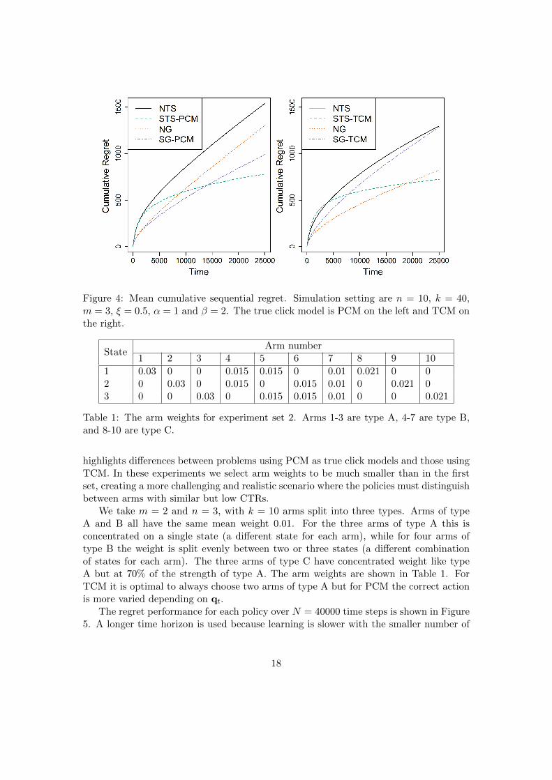
Figure 4: Mean cumulative sequential regret. Simulation setting are n = 10, k = 40,m = 3, ξ = 0.5, α = 1 and β = 2. The true click model is PCM on the left and TCM onthe right.

StateArm number

1 2 3 4 5 6 7 8 9 10

1 0.03 0 0 0.015 0.015 0 0.01 0.021 0 02 0 0.03 0 0.015 0 0.015 0.01 0 0.021 03 0 0 0.03 0 0.015 0.015 0.01 0 0 0.021

Table 1: The arm weights for experiment set 2. Arms 1-3 are type A, 4-7 are type B,and 8-10 are type C.

highlights differences between problems using PCM as true click models and those usingTCM. In these experiments we select arm weights to be much smaller than in the firstset, creating a more challenging and realistic scenario where the policies must distinguishbetween arms with similar but low CTRs.

We take m = 2 and n = 3, with k = 10 arms split into three types. Arms of typeA and B all have the same mean weight 0.01. For the three arms of type A this isconcentrated on a single state (a different state for each arm), while for four arms oftype B the weight is split evenly between two or three states (a different combinationof states for each arm). The three arms of type C have concentrated weight like typeA but at 70% of the strength of type A. The arm weights are shown in Table 1. ForTCM it is optimal to always choose two arms of type A but for PCM the correct actionis more varied depending on qt.

The regret performance for each policy over N = 40000 time steps is shown in Figure5. A longer time horizon is used because learning is slower with the smaller number of

18

Figure 5: Mean cumulative sequential regret for experiment set 2. A fixed arm scenariowith small weights is used. The true click model is PCM on the left and TCM on theright.

clicks that come with low CTRs. For all click models the two greedy policies struggle.With PCM the two TS-based policies are very similar. This is unsurprising since withlow expected CTRs the reward function under PCM is a similar function to additiverewards and in this setting SEQ and NAI act similarly. For TCM the results are moreunexpected with NTS outperforming STS, although with a similar pattern.

Figure 6 shows the arm types chosen by each policy at times t ∈ {35001, . . . , 40000}.In the TCM problem it is optimal to choose arms of type A but the other policieschoose arms from both of the other groups. The STS-TCM policy has chosen a higherpercentage of optimal arms than NTS, showing that it doing better by the end of thesimulation but, because the available reward is small, its cumulative regret performanceis only catching slowly. In the PCM problem the optimal mix of arms consists of armsfrom all groups. Here the TS policies have a similar mix of types to the Oracle policywhile the greedy policies select from type B (the all-rounders) too often, indicating alack of adequate learning.

Overall, it appears from the experiments that both exploration algorithm and setchoosing method are important for good performance. Which is more important variesbetween experiment, especially for short term performance. However, over the longerterm, while the naive set choosing method can do quite well on some problems, using agreedy exploration algorithm consistently results in under-performance.

19

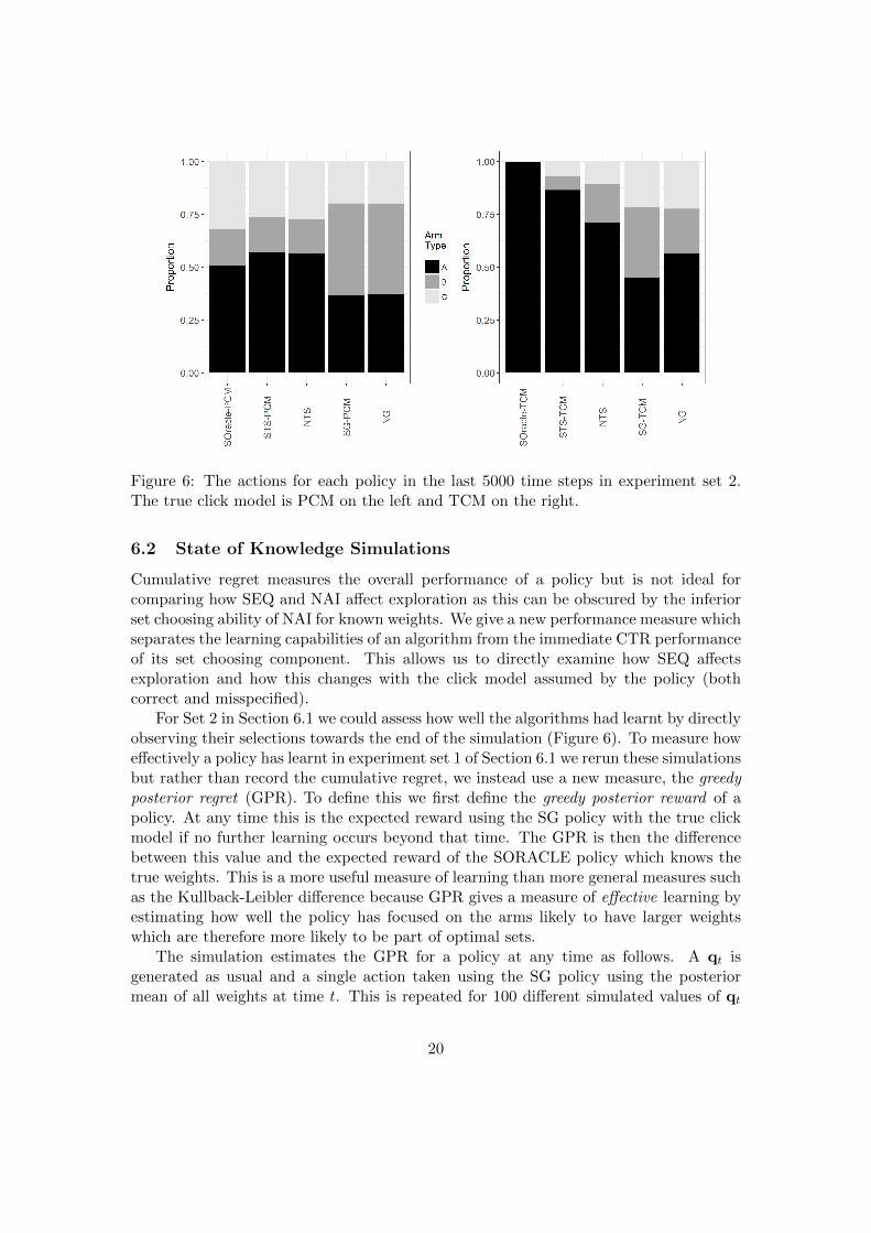
Figure 6: The actions for each policy in the last 5000 time steps in experiment set 2.The true click model is PCM on the left and TCM on the right.

6.2 State of Knowledge Simulations

Cumulative regret measures the overall performance of a policy but is not ideal forcomparing how SEQ and NAI affect exploration as this can be obscured by the inferiorset choosing ability of NAI for known weights. We give a new performance measure whichseparates the learning capabilities of an algorithm from the immediate CTR performanceof its set choosing component. This allows us to directly examine how SEQ affectsexploration and how this changes with the click model assumed by the policy (bothcorrect and misspecified).

For Set 2 in Section 6.1 we could assess how well the algorithms had learnt by directlyobserving their selections towards the end of the simulation (Figure 6). To measure howeffectively a policy has learnt in experiment set 1 of Section 6.1 we rerun these simulationsbut rather than record the cumulative regret, we instead use a new measure, the greedyposterior regret (GPR). To define this we first define the greedy posterior reward of apolicy. At any time this is the expected reward using the SG policy with the true clickmodel if no further learning occurs beyond that time. The GPR is then the differencebetween this value and the expected reward of the SORACLE policy which knows thetrue weights. This is a more useful measure of learning than more general measures suchas the Kullback-Leibler difference because GPR gives a measure of effective learning byestimating how well the policy has focused on the arms likely to have larger weightswhich are therefore more likely to be part of optimal sets.

The simulation estimates the GPR for a policy at any time as follows. A qt isgenerated as usual and a single action taken using the SG policy using the posteriormean of all weights at time t. This is repeated for 100 different simulated values of qt

20

Figure 7: Mean greedy posterior regret for TS-based policies with PCM (left) and TCM(right). Simulation setting are n = 10, k = 40, m = 3, ξ = 0.5, α = 1 and β = 2.

for each run of the original simulation. The GPR at time t is the mean regret over the100 qt values.

The GPR over time for TS-based policies with PCM and TCM as the true clickmodel are shown in Figure 7. It also tests misspecified click models for SEQ-basedpolicies. NTS ignores click model. The time axis starts at t = 1000 because GPR valuesare high at early times before the policies have had much time to learn. GPR values forthe Greedy-based policies are much higher and so these are shown on a separate plot inFigure 8 with just NTS for comparison. We will consider the TS-based policies firstbefore moving on to the Greedy-based policies. For PCM all of the TS policies are verysimilar. On TCM both STS policies do better than NTS with STS-TCM best of all.Generally, all the TS-based policies appear robust to variation in the click model.

The learning for the Greedy-based policies is, as expected, clearly worse than forTS but, in addition, there is large variation among the Greedy variants. In particularSG-TCM learns poorly on both PCM and TCM. This explains the poor regret for SGwith TCM in Section 6.1, showing that the problem is with the click model assumed bythe policy rather than the true click model. So, for Greedy-based policies, it is morerobust for learning to assume PCM.

The results here and the regret simulations in Section 6.1 suggest that, in addition tosuperior exploitation, STS also learns as effectively as NTS and is better for a correctlyspecified TCM.

21

Figure 8: Mean greedy posterior regret for Greedy-based policies with PCM (left) andTCM (right). Simulation setting are n = 10, k = 40, m = 3, ξ = 0.5, α = 1 and β = 2.The NTS policy is shown for comparison.

7 Discussion

In this paper we formulated the multiple advert problem and gave a solution methodwhich combined bandit algorithms with submodular set-choosing methods in a Bayesiansetting. The setting is a challenging one, principally due to the twin uncertainties con-cerning: (i) the topic and quality of each advert and, (ii) the preferences of the users.The first of these can be learnt over time by observing user click behaviour but thesecond uncertainty is inherent due to an unobservable user state. The resulting contex-tual bandit problem, our analysis and proposed methods will have wider application inproblems where there is state uncertainty in addition to the usual arm uncertainty.

The model used here is structurally simple but can encompass greater complexityin application through the topic preference vector q which could contain considerableinformation since model and solution methods are practical with very large q . A possiblelimitation of the model is that a user state is given by a single x. An easily implementedextension would be to record the user state as a very sparse vector the same length asw and model clicks with some function of these two vectors e.g. the probit of the dotproduct. A similar model for single advert CTR prediction that has been implementedin commercial web search is given in Graepel et al. (2010).

We did not compare our approach with existing methods because none were designedfor our problem formulation and make inappropriate assumptions for our specific model.A formal bound on finite time regret would be desirable but the difficulty of our problemwith a stochastic latent state in addition to stochastic arms makes this impractical.In particular the approximate Bayesian scheme does not give guarantees of accurate

22

convergence of weight beliefs so regret growth cannot be usefully bounded.The simulations in Section 6.1 suggest exploration of weights will be slow as the

problem is scaled up. This is mainly due to there being kn parameters to learn com-pared to just k for the standard MAB but also because the unknown x makes feedbackless informative than normal. Therefore slow exploration is a feature of the problemrather than the methods used and so is unavoidable unless greater assumptions (e.g. de-pendence between weights or arms) are made on the structure of the weights. There areexamples of this in bandit problems (e.g. Yue & Guestrin 2011) but the intention in thiswork is to use a model that is as general as possible, only adding in such assumptions ifit is clear they are valid and necessary. Furthermore we anticipate that exploration maynot be a problem in practice due to the high rate of observations and by using priorsthat represent existing knowledge of likely arm CTRs. This ability to incorporate priorknowledge is a strong advantage of the proposed Bayesian scheme.

8 Acknowledgements

This work was funded by a Google Faculty Research Award. James Edwards was sup-ported by the EPSRC funded EP/H023151/1 STOR-i CDT.

A Derivations for Section 4

A.1 Updating Equations for Arm Weights

PCM. The joint distribution for all weights given a feedback step is updated as givenbelow. In the following note that p(·|q, x) simplifies to p(·|x) and that p(wA, x|q, A) =p(wA)qx since x is independent of wA. The posterior belief for the weights after a useraction is,

p(wA|y,m∗,q, A) =n∑x=1

p(wA, x|y,m∗,q, A)

=n∑x=1

p(y,m∗|wA, x,q, A)p(wA, x|q, A)

p(y,m∗|q, A)

=1

p(y,m∗|q, A)

n∑x=1

{[(wam∗ ,x)y

∏a∈A′

(1− wa,x)

]p(wA)qx

}

=p(wA)

p(y,m∗|q, A)

n∑x=1

[qx(wam∗ ,x)y

∏a∈A′

(1− wa,x)

].

TCM. The updating equation for wA for TCM is similar to that for PCM except

23

that p(y,m∗|wA, x,q) changes due to the user threshold u:

p(wA|y,m∗,q, A) =n∑x=1

p(wA, x|y,m∗,q, A)

=

n∑x=1

p(y,m∗|wA, x,q, A)p(wA, x|q, A)

p(y,m∗|q, A)

=p(wA)

p(y,m∗|q, A)

∫ 1

u=0

n∑x=1

[qx(1{wam∗ ,x>u}

)y∏a∈A′

1{wa,x≤u}

]du. (4)

A.2 Derivation of q

The posterior q = (q1, . . . , qn) depends on WA, y, m∗, q and A. For ease of reading therest of this section will use w and W to respectively stand for wA and WA. Bayes The-orem will be used to condition the outcome on x which allows the use of the conditionalindependence of arms under PCM to factorise to a simple formula.

qx = p(x |W, y,m∗,q, A)

=

∫p(x,w |W, y,m∗, a, A) dw

=

∫p(x | w, y,m∗,q, A)p(w |W, y,m∗,q, A) dw

=

∫p(y,m∗ | x,w,q, A)p(x | w,q, A)

p(y,m∗ | w,W,q, A)p(w |W, y,m∗,q, A) dw,

Then, substituting in

p(w |W, y,m∗,q, A) =p(w, y,m∗ |W,q, A)

p(y,m∗ |W,q, A)

=p(y,m∗ | w,W,q, A)p(w |W)

p(y,m∗ |W,q, A),

and cancelling gives

qx =

∫p(y,m∗ | x,w,q, A)p(x | w,q, A)p(w |W)

p(y,m∗ |W,q, A)dw

= qx

∫p(y,m∗ | x,w,q, A)p(w |W)∑

x qx∫p(y,m∗ | x, w,q, A)p(w |W) dw

dw, (5)

where the last step uses p(x | w,q, A) = p(x | q) = qx.It remains to find

∫p(y,m∗ | x,w,q, A)p(w | W) dw. Under PCM this is easily

found since, given x, the probability of clicking any arm a considered by the user is the

24

same as its independent click probability (as though it were the only arm in the set) andis independent from all weights except wa,x. That is, for a single arm a,∫

p(y,m∗ | x,w,q, A)p(w |W) dw =

∫p(y,m∗ | x,wa,x,q, A)p(wa,x |Wa,x) dwa,x

= (µa,x)y(1− µa,x)(1−y), (6)

where µa,x =αa,x

αa,x+βa,xis the expectation of Wa,x. Under PCM, the outcome of any arm,

given it is considered by the user, is independent of the other arms so (5) and (6) canbe combined to give

qx = qx(µam∗ ,x)y

∏a∈A′(1− µa,x)∑n

j=1[qj(µam∗ ,x)y∏a∈A′(1− µa,x)]

.

A.3 Updating for TCM with Known x

Adapting (4) in Section A.1, the updating for known x under TCM is

p(wA|y,m∗, x) =p(wA)

p(y,m∗|q)

∫ 1

u=0qx(1{wam∗ ,x>u}

)y∏a∈A′

1{wa,x≤u}du

=qxp(wA)

p(y,m∗|q)

∫ 1

u=0(1{wam∗ ,x>u}

)y1{u>maxa∈A′ (wa,x)}du

=qxp(wA)

p(y,m∗|q)

[(wam∗ ,x)y −max

a∈A′(wa,x)

].

B Lemma B.1

The following lemma is used in the proof of Theorem 5.1 which is given in Appendix C.Both this lemma and the proof of Theorem 5.1 use the following notation.

Let RTS(a,Wa,t,qt | It) = qt · wa,t denote the stochastic index for the multi-ple action Thompson sampling policy for a single arm a where each wa,t,x ∼ Wa,t,x.Then under SEQ the arm chosen in slot one is the one with the highest index: at,1 =argmaxa∈AR

TS(a,Wa,t,qt|It).

Lemma B.1. Let τa,T be the set of times t = 1, . . . , T at which a ∈ At. Let q∗ =inft,x Pr(qt,x = 1) and w∗ = maxa∈A,xwa,x and, from these, set η = q∗(1 − w∗)m. Ifq∗ > 0 then under the deterministic updating scheme given in Section 4.2 using anyclick model from Section 3.2,

Pr

(RTS(a,Wa,T ,qT | It) ≤

1

1 + η − δ1+ δ2

)→ 1 as |τa,T | → ∞

for any a ∈ A and any δ1, δ2 such that η > δ1 > 0 and δ2 > 0.

25

Proof. For any a ∈ A, x = 1, . . . , n we will give bounds for expected rate at whichαa,t,x and βa,t,x increase as the arm a is selected over time (an upper bound for αa,t,xand a lower bound for βa,t,x). This will give an asymptotic upper bound less than 1 oneach posterior mean µa,t,x = E [Wa,t,x] as |τa,t| → ∞. Showing that V ar(Wa,t,x)→ 0 as|τa,t| → ∞ then gives the required result. Throughout, a is an arbitrary arm in A andx an arbitrary state in {1, . . . , n}.

Let αa,0,x and βa,0,x be values of the parameters of the Beta prior placed on wa,x,then an upper bound for αa,T,x, T ≥ 1 is simply

αa,T,x ≤ αa,0,x + |τa,T | (7)

since αa,T,x can only increase by at most one at times when when a ∈ At and is un-changing at other times.

For a lower bound on E [βa,T,x] we consider only times when a ∈ At, qt,x = 1 andyt = 0. Then yt = 0 guarantees that arm a is considered by the user and qt,x = 1 meansthe failure to click can be attributed to wa,x. Hence, for t ≥ 1,

βa,t+1,x | (qt,x = 1, yt = 0, a ∈ At, βa,t,x) = βa,t,x + 1. (8)

At all times βa,t+1,x ≥ βa,t,x since the β parameters cannot decrease. For PCM,

Pr(yt = 0 | qt,x = 1, At,wAt) =∏b∈At

(1− wb,x)

which is no larger than the corresponding probability for TCM. The probability that yt =0 can therefore be bounded below. Let w∗ = maxb∈A,xwb,x and q∗ = mint,x Pr(qt,x = 1)then for any At ⊂ A,

Pr(yt = 0 | At,wA) ≥ q∗(1− w∗)m. (9)

We can now give a lower bound on E [βa,T,x | I1] where the expectation is joint over allqt, yt, m

∗t for t = 1, . . . , T , and I1 is just the priors for W. Using (8) and (9), we have

at any time T ,

E[βa,T,x | I1] ≥ βa,0,x +∑t∈τa,T

[Pr(qt,x = 1) Pr(yt = 0 | qt,x = 1, a ∈ At,wAt)

]≥ |τa,T |q∗(1− w∗)m. (10)

Let η = q∗(1 − w∗)m and note that η > 0 since w∗ < 1 by the problem definition andq∗ > 0 by the assumption given in the statement of the Lemma. Combining (7) and (10)gives, for any τa,T ,

E[βa,T,xαa,T,x

| I1]≥ 1

αa,0,x + |τa,T |E [βa,T,x | I1]

≥|τa,T |η

αa,0,x + |τa,T |

26

and so by the strong law of large numbers, for sufficiently large |τa,T | and conditional onI1,

βa,T,xαa,T,x

≥|τa,T |η

αa,0,x + |τa,T |→ η . (11)

Note that

µa,T,x =αa,T,x

αa,T,x + βa,T,x=

1

1 +βa,T,x

αa,T,x

,

and so from (11),

Pr

(µa,T,x ≤

1

1 + η − δ1

)→ 1 as |τa,T | → ∞ (12)

for any δ1 such that η > δ1 > 0.Then, using the variance of a Beta distribution and (10) we have

V ar(Wa,T,x) =αa,T,xβa,T,x

(αa,T,x + βa,T,x)2(αa,T,x + βa,T,x + 1)

<(αa,T,x + βa,T,x)2

(αa,T,x + βa,T,x)2(αa,T,x + βa,T,x + 1)

=1

(αa,T,x + βa,T,x + 1)→ 0 as |τa,T | → ∞,

and so for any δ2 > 0 the sampled wa,T,x ∼Wa,T,x satisfy

Pr (wa,T,x ≤ µa,T,x + δ2)→ 1 as |τa,T | → ∞. (13)

By definition RTS(a,Wa,t,qt | It) =∑n

x=1(qt,xwa,t,x) ≤ maxx wa,t,x where wa,t,x ∼Wa,t,x. Therefore, to complete the proof it is sufficient that Pr(wa,T,x < 1/(1 + η− δ1) +δ2) → 1 as |τa,T | → ∞ for all a ∈ A, x = 1, . . . n and any δ1, δ2 such that η > δ1 > 0and δ2 > 0, which follows from (12) and (13).

C Proof of Theorem 5.1

The proof will assume that there is a non-empty set of arms AF ⊂ A whose membersare sampled finitely often as t→∞ and show that this leads to a contradiction. Underthis assumption

∑b∈AF

|τb,∞| < ∞ and so there exists a finite time M = maxb∈AFτb,t

even as t→∞.Let AI = A \ AF be the set of arms sampled infinitely often (which must be non-

empty). Let w∗ = maxa∈A,xwa,x and η = q∗(1 − w∗)m as in the proof of Lemma B.1.Note that η > 0 since w∗ < 1 by the problem definition and q∗ > 0 by the givencondition. Then fix some 0 < δ1 < η and 0 < δ2 < 1− 1/(1 + η − δ1). Then by LemmaB.1 for all a ∈ AI ,

Pr

(RTS(a,Wa,t,qt) ≤

1

1 + η − δ1+ δ2

)→ 1 as t→∞.

27

So there exists a finite random time T > M such that

Pr

(RTS(a,Wa,t,qt) ≤

1

1 + η − δ1+ δ2

)> 1− δ2 for t > T, ∀a ∈ AI . (14)

Let ε = minb∈AF[Pr(RTS(b,Wb,T ,qT | IT ) > 1/(1 + η − δ1) + δ2)]. Then for all t > T ,

b ∈ AF we have

Pr

(RTS(b,Wb,t,qt | It) >

1

1 + η − δ1+ δ2

)≥ ε, (15)

since no arm in AF is selected at times t > T > M and so Wb,t is unchanged over thesetimes. We know that ε > 0 since Pr(wb,T,x > 1/(1 + η+ δ1) + δ2) > 0 for all b, x because1/(1 + η − δ1) + δ2 < 1 and Wb,T,x is a Beta distribution with support (0, 1).

Combining (14) and (15),

Pr[RTS(b,Wb,t,qt | It) > RTS(a,Wa,t,qt | It),∀a ∈ A

]> ε(1− δ2) (16)

for all t > T . Therefore

∞∑t=T

Pr(b ∈ At for some b ∈ AF ) >

∞∑t=T

ε(1− δ2)|AI | =∞.

Using the Extended Borel-Cantelli Lemma (Corollary 5.29 of Breiman 1992) it followsthat

∑b∈AF

|τb,∞| = ∞ which contradicts the assumption that |τb,∞| is finite for allb ∈ AF . Therefore some arm in AF is selected infinitely often and since AF was ofarbitrary size it follows that AF = ∅.

References

Agrawal, R., Gollapudi, S., Halverson, A. & Ieong, S. (2009), Diversifying search results,in ‘ACM Conference on Web Search and Data Mining (WSDM)’, ACM, pp. 5–14.

Ahmed, M. T. & Kwon, C. (2014), ‘Optimal contract-sizing in online display advertisingfor publishers with regret considerations’, Omega 42(1), 201–212.

Auer, P. (2002), ‘Using confidence bounds for exploitation-exploration trade-offs’, TheJournal of Machine Learning Research 3, 397–422.

Auer, P., Cesa-Bianchi, N. & Fischer, P. (2002), ‘Finite-time analysis of the multiarmedbandit problem’, Machine Learning 47(2), 235–256.

Balseiro, S. R., Feldman, J., Mirrokni, V. & Muthukrishnan, S. (2014), ‘Yield optimiza-tion of display advertising with ad exchange’, Management Science 60(12), 2886–2907.

Breiman, L. (1992), Probability, Society for Industrial and Applied Mathematics,Philadelphia, PA.

28

Cappe, O. & Moulines, E. (2009), ‘On-line expectation–maximization algorithm for la-tent data models’, Journal of the Royal Statistical Society, B 71(3), 593–613.

Chapelle, O., Manavoglu, E. & Rosales, R. (2015), ‘Simple and scalable response predic-tion for display advertising’, ACM Transactions on Intelligent Systems and Technology(TIST) 5(4), 61.

Chen, W., Wang, Y. & Yuan, Y. (2013), Combinatorial multi-armed bandit: Generalframework and applications, in ‘Proceedings of the 30th International Conference onMachine Learning’, pp. 151–159.

Chen, Y.-J. (2017), ‘Optimal dynamic auctions for display advertising’, Operations Re-search 65(4), 897–913.

Chen, Y., Pavlov, D. & Canny, J. F. (2009), Large-scale behavioral targeting, in ‘Pro-ceedings of the 15th ACM SIGKDD international conference on Knowledge discoveryand data mining’, ACM, pp. 209–218.

Chuklin, A., Markov, I. & Rijke, M. d. (2015), Click models for web search, Vol. 7,Morgan & Claypool Publishers.

Craswell, N., Zoeter, O., Taylor, M. & Ramsey, B. (2008), An experimental comparisonof click position-bias models, in ‘Proceedings of the International Conference on WebSearch and Web Data Mining’, ACM, pp. 87–94.

Edwards, J. A. & Leslie, D. S. (2018), Diversity as a Response to User PreferenceUncertainty, World Scientific, chapter 4, pp. 55–68.

El-Arini, K., Veda, G., Shahaf, D. & Guestrin, C. (2009), Turning down the noise in theblogosphere, in ‘ACM Conference on Knowledge Discovery and Data Mining’, ACM,pp. 289–298.

Fridgeirsdottir, K. & Najafi-Asadolahi, S. (2018), ‘Cost-per-impression pricing for dis-play advertising’, Operations Research 66(3), 653–672.

Gittins, J. C., Glazebrook, K. D. & Weber, R. (2011), Multi-armed bandit allocationindices, second edn, John Wiley & Sons, Chichester, UK.

Graepel, T., Candela, J. Q., Borchert, T. & Herbrich, R. (2010), Web-scale Bayesianclick-through rate prediction for sponsored search advertising in Microsoft’s Bingsearch engine, in ‘Proceedings of the 27th International Conference on Machine Learn-ing’, pp. 13–20.

Hauser, J. R., Urban, G. L., Liberali, G. & Braun, M. (2009), ‘Website morphing’,Marketing Science 28(2), 202–223.

Hillard, D., Schroedl, S., Manavoglu, E., Raghavan, H. & Leggetter, C. (2010), Improv-ing ad relevance in sponsored search, in ‘Proceedings of the third ACM internationalconference on Web search and data mining’, ACM, pp. 361–370.

29

Hojjat, A., Turner, J., Cetintas, S. & Yang, J. (2017), ‘A unified framework for thescheduling of guaranteed targeted display advertising under reach and frequency re-quirements’, Operations Research 65(2), 289–313.

Larsen, T., Leslie, D. S., Collins, E. J. & Bogacz, R. (2010), ‘Posterior weighted rein-forcement learning with state uncertainty’, Neural Computation 22(5), 1149–1179.

Li, L., Chu, W., Langford, J. & Schapire, R. E. (2010), A contextual-bandit approach topersonalized news article recommendation, in ‘Proceedings of the 19th InternationalConference on World Wide Web’, ACM, pp. 661–670.

May, B. C., Korda, N., Lee, A. & Leslie, D. S. (2012), ‘Optimistic Bayesian sampling incontextual-bandit problems’, Journal of Machine Learning Research 13(1), 2069–2106.

McMahan, H. B., Holt, G., Sculley, D., Young, M., Ebner, D., Grady, J., Nie, L., Phillips,T., Davydov, E., Golovin, D., Chikkerur, S., Liu, D., Wattenberg, M., Hrafnkelsson,A. M., Boulos, T. & Kubica, J. (2013), Ad click prediction: a view from the trenches,in ‘Proceedings of the 19th ACM SIGKDD international conference on Knowledgediscovery and data mining’, ACM, pp. 1222–1230.

Najafi-Asadolahi, S. & Fridgeirsdottir, K. (2014), ‘Cost-per-click pricing for display ad-vertising’, Manufacturing & Service Operations Management 16(4), 482–497.

Nemhauser, G. L. & Wolsey, L. A. (1978), ‘Best algorithms for approximating the max-imum of a submodular set function’, Mathematics of Operations Research 3(3), 177–188.

Radlinski, F., Kleinberg, R. & Joachims, T. (2008), Learning diverse rankings withmulti-armed bandits, in ‘Proceedings of the 25th international conference on Machinelearning’, ACM, pp. 784–791.

Ricci, F., Rokach, L. & Shapira, B. (2011), Recommender Systems Handbook, SpringerUS, Boston, MA.

Richardson, M., Dominowska, E. & Ragno, R. (2007), Predicting clicks: estimating theclick-through rate for new ads, in ‘Proceedings of the 16th international conference onWorld Wide Web’, ACM, pp. 521–530.

Rusmevichientong, P. & Williamson, D. P. (2006), An adaptive algorithm for selectingprofitable keywords for search-based advertising services, in ‘Proceedings of the 7thACM Conference on Electronic Commerce’, ACM, pp. 260–269.

Russo, D. & Van Roy, B. (2014), ‘Learning to optimize via posterior sampling’, Mathe-matics of Operations Research 39(4), 1221–1243.

Schwartz, E. M., Bradlow, E. T. & Fader, P. S. (2017), ‘Customer acquisition via displayadvertising using multi-armed bandit experiments’, Marketing Science 36(4), 500–522.

30

Streeter, M., Golovin, D. & Krause, A. (2009), Online learning of assignments, in ‘Ad-vances in Neural Information Processing Systems’, pp. 1794–1802.

Whittle, P. (1988), ‘Restless bandits: Activity allocation in a changing world’, Journalof Applied Probability 25, 287–298.

Yan, J., Liu, N., Wang, G., Zhang, W., Jiang, Y. & Chen, Z. (2009), How much canbehavioral targeting help online advertising?, in ‘Proceedings of the 18th internationalconference on World wide web’, ACM, pp. 261–270.

Yue, Y. & Guestrin, C. (2011), Linear submodular bandits and their application to di-versified retrieval, in ‘Advances in Neural Information Processing Systems’, pp. 2483–2491.

31