Embed Size (px)
Citation preview
University of Missouri, St. LouisIRL @ UMSL
Dissertations UMSL Graduate Works
8-4-2014
Selecting the best supply chain strategy: When is amisalignment of product type and strategyappropriate, how do changes in expected demandimpact strategies, and should the strategy of aproduct change over its life-cycle?William EllegoodUniversity of Missouri-St. Louis, [email protected]
Follow this and additional works at: https://irl.umsl.edu/dissertation
Part of the Business Commons
This Dissertation is brought to you for free and open access by the UMSL Graduate Works at IRL @ UMSL. It has been accepted for inclusion inDissertations by an authorized administrator of IRL @ UMSL. For more information, please contact [email protected].
Recommended CitationEllegood, William, "Selecting the best supply chain strategy: When is a misalignment of product type and strategy appropriate, how dochanges in expected demand impact strategies, and should the strategy of a product change over its life-cycle?" (2014). Dissertations.226.https://irl.umsl.edu/dissertation/226

Revision July 23, 2014 Copyright, William A. Ellegood, 2014
Selecting the best supply chain strategy
When is a misalignment of product type and strategy
appropriate, how do changes in expected demand impact strategies, and should the strategy of a product
change over its life-cycle?
William Ellegood
M.B.A, Ball State University – Muncie, IN, 1999
B.S., Mechanical Engineering, GMI Engineering and Management Institute – Flint, MI,
1994
A Thesis Submitted to The Graduate School at the University of Missouri – St. Louis in
partial fulfillment of the requirements for the degree Ph.D. in Business Administration with
an emphasis in Logistics and Supply Chain Management
Advisory Committee
James F. Campbell, Ph.D.
Co-Chairperson
Donald C. Sweeney II, Ph.D.
Co-Chairperson
Gerald Y. Gao, Ph.D.
Ray Mundy, Ph.D.

ii Copyright, William A. Ellegood, 2014 Revision July 23, 2014
Table of Contents
Table of Figures ................................................................................................................. iv
Table of Tables ................................................................................................................ viii
Abstract ............................................................................................................................... x
1. Introduction ................................................................................................................. 1
1.1 Alignment .................................................................................................................. 2
1.2 Supply chain strategy ................................................................................................ 5
1.3 Product life cycle and supply chain strategy ............................................................. 6
1.4 Methodology ........................................................................................................... 10
1.5 Outline ..................................................................................................................... 12
2. Literature review ........................................................................................................ 14
2.1 Supply chain strategy selection framework ............................................................ 14
2.2 Examining the Fisher Model and supply chain strategy alignment ........................ 23
2.3 Lean/leagile/agile .................................................................................................... 32
2.4 Product life cycle and supply chain strategy ........................................................... 38
2.5 Supply chain strategy selection and improvement .................................................. 42
2.6 Analytical models for supply chain strategy selection ............................................ 47
2.7 Net present value and supply chain management ................................................... 49
2.8 Summary ................................................................................................................. 51
3. Analytical model........................................................................................................ 54
3.1 Notation ................................................................................................................... 54
3.2 Model description .................................................................................................... 56
3.3 Model construction .................................................................................................. 68
3.4 Supply chain strategy model construction .............................................................. 70
3.5 Model analysis framework ...................................................................................... 74
4. Examining the Fisher Model (lean and agile SCS only) ........................................... 78
4.1 Problem description ................................................................................................. 78
4.2 Scenario analysis ..................................................................................................... 89
4.2.1 Low demand forecast error ............................................................................... 92
4.2.2 High demand forecast error .............................................................................. 95

Revision July 23, 2014 Copyright, William A. Ellegood, 2014 iii
4.3 Sensitivity analysis .................................................................................................. 99
4.3.1 Total production cost to total order processing cost ......................................... 99
4.3.2 Average daily demand .................................................................................... 105
4.3.3 Supply side lead time ...................................................................................... 110
4.3.4 Agile SCS service level .................................................................................. 115
4.4 Summary ............................................................................................................... 120
5. Supply chain strategy selection ............................................................................... 124
5.1 Problem description ............................................................................................... 124
5.2 Scenario analysis ................................................................................................... 128
5.3 Sensitivity analysis ................................................................................................ 132
5.3.1 Expected demand changes over time .............................................................. 133
5.3.2 Demand forecast error and demand changes with time .................................. 142
5.4 Summary ............................................................................................................... 150
6. Supply chain strategy selection for product life cycle ............................................. 153
6.1 Problem description ............................................................................................... 153
6.2 Scenario analysis ................................................................................................... 164
6.3 Examples ............................................................................................................... 178
6.3.1 Functional product .......................................................................................... 178
6.3.2 Hybrid product ................................................................................................ 184
6.3.3 Innovative product .......................................................................................... 188
6.4 Agile SCS to a lean SCS ....................................................................................... 191
6.4.1 High RMP ....................................................................................................... 192
6.4.2 Medium RMP ................................................................................................. 194
6.4.3 Low RMP ........................................................................................................ 195
6.5 Summary ............................................................................................................... 197
7. Conclusion ............................................................................................................... 199
7.1 Findings ................................................................................................................. 200
7.2 Managerial insights ............................................................................................... 203
7.3 Contributions ......................................................................................................... 205
7.4 Limitations ............................................................................................................ 206
7.5 Opportunities for future research .......................................................................... 207

iv Copyright, William A. Ellegood, 2014 Revision July 23, 2014
Works cited ..................................................................................................................... 208
Table of Figures
Figure 1.1: Matching supply chain strategy to product type (Source: Fisher, 1997) .......... 2
Figure 1.2: Classical product life cycle (Source: Rink and Swan, 1979) ........................... 7
Figure 1.3: Alignment of PLC, Fisher Model, and SCS based on manufacturing
paradigms ............................................................................................................................ 8
Figure 1.4: Three echelon supply chain with two inventory points .................................. 11
Figure 3.1: Three echelon supply chain with two inventory points .................................. 57
Figure 3.2: Timing of manufacturer and supplier costs relative to order delivery time ... 63
Figure 3.3: Actual demand normally distributed about expected demand ....................... 65
Figure 3.4: Scenario analysis considering RMP, lean index, demand forecast error, and
cost of capital. ................................................................................................................... 77
Figure 4.1: SCS with the lowest Total Cost (Lean and Agile only) ................................. 90
Figure 4.2: Value of when one characteristic is varied and the other three are fixed
with low RMP, low lean index, high cost of capital, and low demand forecast error. ..... 93
Figure 4.3: Cost of capital that makes as a function of the value of
( ) and the lean index value when demand forecast error is low as described in
Table 3.4. .......................................................................................................................... 95
Figure 4.4: Value of when one characteristic is varied and the other three are fixed
with RMP high, lean index medium, cost of capital low, and demand forecast error high.
........................................................................................................................................... 97
Figure 4.5: Cost of capital that makes as a function of the value of
( ) and the lean index value when demand forecast error is high as described in
Table 3.4. .......................................................................................................................... 98
Figure 4.6: Value of with respect to the ratio of total production cost to total order
processing cost for different RMP levels. ....................................................................... 101
Figure 4.7: Value of with respect to the ratio of total production cost to total order
processing cost for different demand forecast error levels. ............................................ 102

Revision July 23, 2014 Copyright, William A. Ellegood, 2014 v
Figure 4.8: Value of with respect to the ratio of total production cost to total order
processing cost for different lean index levels. ............................................................... 103
Figure 4.9: Value of with respect to the ratio of total production cost to total order
processing cost for different cost of capital levels. ......................................................... 104
Figure 4.10: Value of with respect to the expected daily demand rate for different
RMP levels. ..................................................................................................................... 106
Figure 4.11: Value of with respect to the expected daily demand rate for different
demand forecast error levels. .......................................................................................... 107
Figure 4.12: Value of with respect to the expected daily demand rate for different
lean index levels. ............................................................................................................. 108
Figure 4.13: Value of with respect to the expected demand rate for different cost of
capital levels.................................................................................................................... 109
Figure 4.14: Value of with respect to the ratio ⁄ for different RMP levels.
......................................................................................................................................... 111
Figure 4.15: Value of with respect to the ratio ⁄ for different demand
forecast error levels. ........................................................................................................ 112
Figure 4.16: Value of with respect to the ratio ⁄ for different lean index
values. ............................................................................................................................. 113
Figure 4.17: Value of with respect to the ratio ⁄ for different cost of capital
levels. .............................................................................................................................. 114
Figure 4.18: Value of with respect to the agile SCS service level for different RMP
levels. .............................................................................................................................. 116
Figure 4.19: Value of with respect to the agile SCS service level for different
demand forecast error levels. .......................................................................................... 117
Figure 4.20: Value of with respect to the agile SCS service level for different lean
index levels. .................................................................................................................... 118
Figure 4.21: Value of with respect to the agile SCS service level for different cost
of capital levels. .............................................................................................................. 119
Figure 4.22: The SCS which results in the lowest Total Cost for all scenarios considered.
......................................................................................................................................... 121

vi Copyright, William A. Ellegood, 2014 Revision July 23, 2014
Figure 5.1: The SCS with the lowest Total Cost (expected demand and demand forecast
error constant) ................................................................................................................. 131
Figure 5.2: Total Cost of each SCS relative to the Total Cost for a lean SCS with high
RMP, high lean index, low demand forecast error, and low cost of capital. .................. 135
Figure 5.3: Total Cost of each SCS relative to the Total Cost for a lean SCS with low
RMP, low lean index, high demand forecast error, and high cost of capital. ................. 135
Figure 5.4: Scenarios wehre the lowest cost SCS is dependent upon the value of . .... 136
Figure 5.5: Group 1: Total Cost of an agilean SCS relative to that of a lean SCS ......... 137
Figure 5.6: Group 2: Total Cost of a leagile SCS relative to that of an agile SCS ......... 139
Figure 5.7: Group 3: Total Cost of an agilean SCS relative to that of an agile SCS ...... 140
Figure 5.8: Group 4: Agile, Agilean SCS vs. Lean SCS ................................................ 141
Figure 5.9: SCS was dependent upon the demand forecast error value .......................... 143
Figure 5.10: Category 1 - RMP-High and Lean Index Medium ..................................... 144
Figure 5.11: Category 2 - RMP-medium and lean index medium .................................. 145
Figure 5.12: Category 3 - RMP-low and lean index medium ......................................... 146
Figure 5.13: Category 4 - RMP-high and lean index-low ............................................... 147
Figure 5.14: Category 5 - RMP-low and lean index-low ................................................ 148
Figure 5.15: Category 6 - RMP-medium and lean index-low ......................................... 149
Figure 5.16: The SCS which results in the lowest Total Cost for all scenarios considered.
......................................................................................................................................... 151
Figure 6.1: Classical product life cycle (Source: Rink and Swan, 1979) ....................... 154
Figure 6.2: Classical PLC from . .............................................................................. 155
Figure 6.3: Classical PLC from with PLC stages. ................................................... 156
Figure 6.4: Demand forecast error and expected demand with respect to time. ............. 166
Figure 6.5: for each level of demand forecast error with respect to time. ...... 166
Figure 6.6: The simple SCS that results in the lowest PLC Total Cost when =100,000
and 5 years for each scenario. .................................................................................. 172
Figure 6.7: The simple SCS that results in the lowest PLC Total Cost when
=1,000,000 and 5 years for each scenario. .......................................................... 172
Figure 6.8: The simple SCS that results in the lowest PLC Total Cost when =100,000
and 2 years for each scenario. .................................................................................. 173

Revision July 23, 2014 Copyright, William A. Ellegood, 2014 vii
Figure 6.9: The simple SCS that results in the lowest PLC Total Cost when
=1,000,000 and 2 years for each scenario. .......................................................... 173
Figure 6.10: The simple SCS that results in the lowest PLC Total Cost when =100,000
and 1 year for each scenario. .................................................................................... 174
Figure 6.11: The simple SCS that results in the lowest PLC Total Cost when
=1,000,000 and 1 year for each scenario. ............................................................ 174
Figure 6.12: Each SCS cost per epoch relative to the simple lean SCS for the functional
product scenario. ............................................................................................................. 181
Figure 6.13: Functional product scenario
per epoch for each SCS. ....................... 182
Figure 6.14: Functional product scenario
per epoch for each SCS. ....................... 182
Figure 6.15: Supply chain strategies of the complex SCS for the hybrid product scenario.
......................................................................................................................................... 185
Figure 6.16: Each SCS cost per epoch relative to the simple lean SCS for the hybrid
product scenario. ............................................................................................................. 185
Figure 6.17: Hybrid product scenario
per epoch for each SCS .............................. 187
Figure 6.18: Hybrid product scenario
per epoch for each SCS. ............................. 187
Figure 6.19: Each SCS cost per epoch relative to the simple agile SCS for the innovative
product scenario. ............................................................................................................. 189
Figure 6.20: Innovative product scenario
per epoch for each SCS ........................ 190
Figure 6.21: Innovative product scenario
per epoch for each SCS. ....................... 190
Figure 6.22: Each SCS cost per epoch relative to the simple lean SCS for a scenario with
high RMP. ....................................................................................................................... 193
Figure 6.23: Each SCS cost per epoch relative to the simple lean SCS for a scenario with
medium RMP. ................................................................................................................. 195
Figure 6.24: Each SCS cost per epoch relative to the simple lean SCS for a scenario with
low RMP. ........................................................................................................................ 196

viii Copyright, William A. Ellegood, 2014 Revision July 23, 2014
Table of Tables
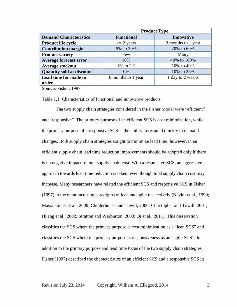
Table 1.1: Characteristics of functional and innovative products....................................... 3
Table 1.2: Characteristics of efficient and responsive supply chains: ................................ 4
Table 2.1: Supply chain strategy classifications from the literature. ................................ 22
Table 2.2: Comparison of lean, agile, and leagile supply chain attributes ....................... 34
Table 3.1: Parameters and coinciding description ............................................................ 56
Table 3.2: Six cost component functions for the Total Cost ............................................. 68
Table 3.3: Time and cost variables for a lean, leagile, and agile supply chain ................. 72
Table 3.4: Characteristic values considered...................................................................... 77
Table 4.1: Legend for the x-axis of Figures 4.6-4.9; showing the ratio of total production
cost to total order processing cost. .................................................................................. 100
Table 4.2: Legend for the x-axis of Figures 4.10-4.14 with expected daily demand and
annual demand. ............................................................................................................... 106
Table 4.3: Legend for the x-axis of Figure 23-26, ratio of the lean SCS supply side lead
time to the agile supply side lead time. ........................................................................... 111
Table 5.1: Change in expected demand for each value of considered with the initial
demand of 275 per day. ................................................................................................... 133
Table 6.1: Characteristics of functional and innovative products: ................................. 165
Table 6.2: Values for characteristics considered in Chapter 6........................................ 168
Table 6.3: Time and cost variables for a lean, leagile, and agile supply chain ............... 169
Table 6.4: Percent difference in the PLC Total Cost of the complex SCS and the best
simple SCS ...................................................................................................................... 177
Table 6.5: Functional product scenario cost ($,000) information for each simple SCS and
the complex SCS by epoch. ............................................................................................ 180
Table 6.6: Hybrid product scenario cost ($,000) information for each simple SCS and the
complex SCS by epoch. .................................................................................................. 184
Table 6.7: Innovative product scenario cost ($,000) information for each simple SCS and
the complex SCS by epoch. ............................................................................................ 188
Table 6.8: High RMP scenario cost ($,000) information for each simple SCS and the
complex SCS by epoch. .................................................................................................. 193

Revision July 23, 2014 Copyright, William A. Ellegood, 2014 ix
Table 6.9: Medium RMP scenario cost ($,000) information for each simple SCS and the
complex SCS by epoch. .................................................................................................. 194
Table 6.10: Low RMP scenario cost ($,000) information for each simple SCS and the
complex SCS by epoch. .................................................................................................. 196
Table 7.1: Summary of hypotheses testing. .................................................................... 201

x Copyright, William A. Ellegood, 2014 Revision July 23, 2014
Abstract
To reduce the total cost of delivering a product to the marketplace, many firms are
going beyond the walls of their organization and working with suppliers and customers to
implement supply chain management (SCM). Fisher (1997) presented a conceptual
model contending that the demand characteristics and supply chain strategy (SCS) of a
product should be aligned for SCM to be successful. This dissertation presents an original
analytical model of a three echelon supply chain to demonstrate under various supply
chain conditions that a “misalignment” between demand characteristics and SCS can
result in a lower total supply chain cost.
In addition to Fisher (1997), the literature includes a number of SCS frameworks
to assist practitioners with identifying the appropriate SCS. However, none have
considered a SCS where the supply side employs an agile strategy and demand side
utilizes a lean strategy; which is denoted as an “agilean” SCS. This dissertation considers
four possible supply chain strategies (lean, agile, leagile, and agilean) and identifies when
each SCS type is most effective at minimizing total supply chain cost.
The demand characteristics of a product typically evolve as a product progresses
through its life-cycle. The literature presents two views concerning whether the SCS of a
product should evolve as the product progresses through its life-cycle. This dissertation
demonstrates that a single SCS employed over the life-cycle of a product is generally a
more effective SCS to minimize total supply chain cost over the life-cycle of a product
than evolving the product’s SCS as it progresses through its life-cycle.

Revision July 23, 2014 Copyright, William A. Ellegood, 2014 1
1. Introduction
The contention that in today’s business environment it is the supply chains of
firms that compete, not the individual firms themselves, and that it is the end consumer
whom ultimately determines the success of a firm’s supply chain (Christopher, 1992) was
made more than 20 years ago. All indications are that this contention is still accurate
today. However, the question for supply chains is, “Which supply chain strategy should
be employed for which product, and should the supply chain strategy evolve as the
demand characteristics of the product evolve over its life-cycle?” Supply chain
management is a managerial concept that encompasses a variety of strategies and those
strategies can differ at different levels of the supply chain, such as the leagile supply
chain strategy, which by one definition combines a lean and an agile supply chain
strategy about a decoupling point. One of the largest challenges a supply chain faces
when implementing supply chain management is the selection of the appropriate supply
chain strategy (SCS) for a product or a family of products. Fisher (1997) stated that for
supply chains to fully realize the benefits of supply chain management (SCM), the supply
chain strategy of a product must be aligned with the demand characteristics of that
product. Figure 1.1 presents Fisher’s general framework for successful alignment of the
product type and SCS. This framework is referred to as “Fisher Model” for the remainder
of this research.

2 Copyright, William A. Ellegood, 2014 Revision July 23, 2014
Figure 1.1: Matching supply chain strategy to product type (Source: Fisher, 1997)
1.1 Alignment
The Fisher Model contends that a functional product requires an efficient supply
chain and an innovative product requires a responsive supply chain. The Fisher Model
classifies products as functional or innovative based on the demand characteristics of the
product. A typical functional product has a long product life cycle (PLC), low
contribution margin, few product varieties, low demand uncertainty, few stock-outs, and
few units sold at a discount at the end of its PLC. In contrast, an innovative product has a
short PLC, high contribution margin, many product varieties, high demand uncertainty,
many stock-outs, and many units sold at a discount at the end of its PLC. To assist
practitioners with determining a product’s type, Fisher (1997) provided guidelines for
seven demand characteristics detailed in Table 1.1.
Match
Mismatch
Responsive
Supply
Chain
Strategy
Efficient
Supply
Chain
Strategy
Functional Product Innovative Product
Mismatch
Match
Revision July 23, 2014 Copyright, William A. Ellegood, 2014 3
Product Type
Demand Characteristics Functional Innovative
Product life cycle >= 2 years 3 months to 1 year
Contribution margin 5% to 20% 20% to 60%
Product variety Few Many
Average forecast error 10% 40% to 100%
Average stockout 1% to 2% 10% to 40%
Quantity sold at discount 0% 10% to 25%
Lead time for made to
order
6 months to 1 year 1 day to 2 weeks
Source: Fisher, 1997
Table 1.1: Characteristics of functional and innovative products.
The two supply chain strategies considered in the Fisher Model were “efficient”
and “responsive”. The primary purpose of an efficient SCS is cost minimization, while
the primary purpose of a responsive SCS is the ability to respond quickly to demand
changes. Both supply chain strategies sought to minimize lead time; however, in an
efficient supply chain lead time reduction improvements should be adopted only if there
is no negative impact to total supply chain cost. With a responsive SCS, an aggressive
approach towards lead time reduction is taken, even though total supply chain cost may
increase. Many researchers have related the efficient SCS and responsive SCS in Fisher
(1997) to the manufacturing paradigms of lean and agile respectively (Naylor et al., 1999;
Mason-Jones et al., 2000; Childerhouse and Towill, 2000; Christopher and Towill, 2001;
Huang et al., 2002; Stratton and Warburton, 2003; Qi et al., 2011). This dissertation
classifies the SCS where the primary purpose is cost minimization as a “lean SCS” and
classifies the SCS where the primary purpose is responsiveness as an “agile SCS”. In
addition to the primary purpose and lead time focus of the two supply chain strategies,
Fisher (1997) described the characteristics of an efficient SCS and a responsive SCS in
4 Copyright, William A. Ellegood, 2014 Revision July 23, 2014
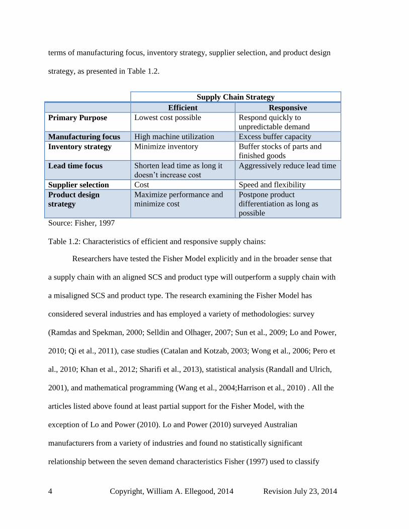
terms of manufacturing focus, inventory strategy, supplier selection, and product design
strategy, as presented in Table 1.2.
Supply Chain Strategy
Efficient Responsive
Primary Purpose Lowest cost possible Respond quickly to
unpredictable demand
Manufacturing focus High machine utilization Excess buffer capacity
Inventory strategy Minimize inventory Buffer stocks of parts and
finished goods
Lead time focus Shorten lead time as long it
doesn’t increase cost
Aggressively reduce lead time
Supplier selection Cost Speed and flexibility
Product design
strategy
Maximize performance and
minimize cost
Postpone product
differentiation as long as
possible
Source: Fisher, 1997
Table 1.2: Characteristics of efficient and responsive supply chains:
Researchers have tested the Fisher Model explicitly and in the broader sense that
a supply chain with an aligned SCS and product type will outperform a supply chain with
a misaligned SCS and product type. The research examining the Fisher Model has
considered several industries and has employed a variety of methodologies: survey
(Ramdas and Spekman, 2000; Selldin and Olhager, 2007; Sun et al., 2009; Lo and Power,
2010; Qi et al., 2011), case studies (Catalan and Kotzab, 2003; Wong et al., 2006; Pero et
al., 2010; Khan et al., 2012; Sharifi et al., 2013), statistical analysis (Randall and Ulrich,
2001), and mathematical programming (Wang et al., 2004;Harrison et al., 2010) . All the
articles listed above found at least partial support for the Fisher Model, with the
exception of Lo and Power (2010). Lo and Power (2010) surveyed Australian
manufacturers from a variety of industries and found no statistically significant
relationship between the seven demand characteristics Fisher (1997) used to classify

Revision July 23, 2014 Copyright, William A. Ellegood, 2014 5
product type and the SCS of the firms. The findings from research examining the Fisher
Model lead to the first question this dissertation considers:
Q1: Under what circumstances does a supply chain with a misaligned SCS and product
type outperform a supply chain with an aligned SCS and product type?
1.2 Supply chain strategy
Researchers have expanded upon the Fisher Model by considering other demand
and/or supply characteristics of a product that could impact the selection of the
appropriate SCS: product uniqueness (Lamming et al., 2000); supply uncertainty (Lee,
2002); level of modularity and postponement (Ernst and Kamrad, 2000); market growth
and technological uncertainty (Randall and Ulrich, 2003); and dominant stage of the PLC
(Cigolini et al., 2004, Vonderembse, 2006). Researchers have found that some products
exhibited demand characteristics of both functional and innovative products (Lee, 2002;
Ernst and Kamrad, 2000; Li and O’Brien, 2001; Christopher and Towill, 2002; Huang et
al. 2002; Cigolini et al., 2004; Wong et al., 2006; and Lo and Power, 2010). Products that
exhibited characteristics of both functional and innovative products may require a SCS
that combines a lean SCS and an agile SCS about a decoupling point, Ernst and Kamrad
(2000) referred to this as a postponed SCS. This dissertation classifies a SCS where a
lean SCS is used upstream of the decoupling point and an agile SCS is used downstream
from the decoupling point as a “leagile SCS”. Ernst and Kamrad (2000) and Lee (2002)
identified a fourth SCS exhibited with some agricultural products, where supply
uncertainty was high and demand uncertainty was low. Both suggested a strategy of
utilizing multiple suppliers to minimize the uncertainty in supply; Ernst and Kamrad
(2000) referred to this strategy as a modularized SCS and Lee (2002) referred to this as a

6 Copyright, William A. Ellegood, 2014 Revision July 23, 2014
risk-hedging SCS. This dissertation considers an alternative strategy, where an agile SCS
is used upstream of the decoupling point and a lean SCS is used downstream from the
decoupling point, denoted as an “agilean SCS”. Therefore, this dissertation considers four
supply chain strategies (lean, leagile, agile, and agilean). This leads to the second
question this dissertation considers:
Q2: Under what combination of supply chain characteristics will each SCS minimize
total supply chain cost?
1.3 Product life cycle and supply chain strategy
A review of the literature reveals two views concerning whether the SCS of a
product should change during the life cycle of the product. The first view is that the SCS
of a product should change as the product progresses through its life cycle (Lamming et
al., 2000; Christopher and Towill, 2000; Childerhouse et al., 2002; Aitken et al., 2003;
Holstrom et al., 2006; Jeong, 2011). The second view is the SCS of a product should be
determined prior to the product’s introduction to the market and the SCS should be fixed
for the entire PLC (Randall and Ulrich, 2001; Cigolini, 2004; Stradtler, 2005; Juttner et
al., 2006; Seuring, 2009). Vonderembse et al. (2006) suggested that the SCS should be
fixed for the PLC of functional and hybrid products, and for an innovative product the
SCS should start with an agile SCS and switch to a leagile SCS or lean SCS for the
maturity and decline stages.
The classical PLC model (Figure 1.2) has four stages: introduction, growth,
maturity, and decline (Cox, 1967). The introduction and growth stages are characterized
by demand instability and higher margin contribution compared to the maturity stage,

Revision July 23, 2014 Copyright, William A. Ellegood, 2014 7
which is characterized by greater demand stability and lower margin contribution (Rink
and Swan, 1979). During the introduction stage of a product, the level of market
acceptance, the diffusion rate of the innovation, and the response of competitors are
impossible to know with certainty. This market instability results in higher demand
uncertainty, similar to an innovative product. During the growth stage, the product
experiences an increase in unit sales per time period at a diminishing rate with
diminishing margin contribution. The diminished growth rate and margin contribution are
the result of increased competition and increased product saturation level in the market
place. Once a product reaches the maturity stage, the product exhibits characteristics
more typical of a functional product as demand stabilizes and forecast accuracy
improves.
Figure 1.2: Classical product life cycle (Source: Rink and Swan, 1979)
Based on Rink and Swan’s (1979) description of the demand characteristics of a
product as it progresses through its life cycle and Fisher’s (1997) demand characteristics
Unit Sales
Introduction Growth Maturity Decline
Time
0

8 Copyright, William A. Ellegood, 2014 Revision July 23, 2014
to identify product type, a product’s demand characteristics will typically evolve from
innovative to functional as it progresses through its life cycle. Accepting the premise that
for supply chain management to be successful the product type must be aligned with the
SCS (Fisher 1997), then the SCS of a product should evolve as the demand
characteristics evolve over the life cycle of the product. One possible evolution of the
appropriate SCS for a product is to start with an agile SCS during the introduction stage,
then evolve to a compound strategy of either leagile SCS or agilean SCS during the
growth stage, and finally evolve to a lean SCS during the maturity stage. Figure 1.3
illustrates a possible alignment of the stages of the PLC, the Fisher Model, and evolving
supply chain strategies.
Figure 1.3: Alignment of PLC, Fisher Model, and SCS based on manufacturing
paradigms
However, the supply chain might incur costs to change the SCS of a product during its
PLC and these costs may exceed the potential benefits to the supply chain from changing
the SCS. In practice we can find examples of very successful firms, for example Dell
Unit Sales
Introduction Growth Maturity Decline
Time
PLC
Fisher Model
SCS
Responsive Efficient
Lean Agile Leagile/Agilean
0

Revision July 23, 2014 Copyright, William A. Ellegood, 2014 9
Inc., which employ a single SCS for the entire life cycle of a product. The leagile SCS
employed by Dell Inc. to manufacture, assemble, and direct ship consumer customized
personal computers has been well documented in the literature (e.g., Simchi-Levi et al.,
2008).
In contrast to the preceding discussion where the SCS may change over the PLC,
the literature concluding the SCS of a product should be determined prior to market
introduction considered supply chain management in a broader sense, as the planning and
management of information and material flows between organizations from raw materials
to the end consumer. Upon further examination of the literature that recommended the
SCS of a product should change during the PLC, more accurate conclusions from the
research concluding the SCS should change over the PLC are (i) the method employed by
the firm to convey demand information to the operations department and (ii) the
operational strategy of a single echelon should change during the PLC. The articles that
concluded the SCS should change over the PLC seem to use an earlier definition for
supply chain management as the planning and management of information and material
flows between the functional departments within an organization (Lamming et al., 2000).
A portion of the definition of “supply chain management” by Council of Supply
Chain Management Professionals is, “… In essence, supply chain management integrates
supply and demand management within and across companies” (CSCMP, n.d.). The
broader definition of supply chain management incorporates the planning and
management of information and material flows both within the organization and between
supply chain members. This dissertation expands on the previous research that considered

10 Copyright, William A. Ellegood, 2014 Revision July 23, 2014
the broader definition of supply chain management. This leads to the third question this
dissertation considers.
Q3: Under what combination of supply chain characteristics does each SCS minimize
total supply chain cost over the life cycle of a product?
1.4 Methodology
Analytical modeling is a valuable technique that may be employed to examine the
overall performance of a system. This modeling method is utilized to provide strategic
managerial insights as to how an objective (e.g. minimize total cost) is impacted as
parameters and/or the relationship of parameters are varied. This dissertation presents an
analytical model for the total supply chain cost when expected demand and demand
forecast error are a function of time. The system is modeled as a three echelon supply
chain (supplier, manufacturer, and customer) with a decoupling point at the manufacturer
and two inventory points, illustrated in Figure 1.4. This formulation allows for four
possible supply chain strategies to be considered: (1) agile SCS, where both the supply
side and demand side of the supply chain utilize an agile strategy; (2) lean SCS, where
both the supply side and demand side of the supply chain utilize a lean strategy; (3)
leagile SCS, where the supply side of the supply chain utilizes a lean strategy and the
demand side of the supply chain employs an agile strategy; and (4) agilean SCS, where
the supply side of the supply chain utilizes an agile strategy and the demand side of the
supply chain employs a lean strategy.

Revision July 23, 2014 Copyright, William A. Ellegood, 2014 11
Figure 1.4: Three echelon supply chain with two inventory points
There are a number of criteria that a firm may adopt for evaluating the
performance of a SCS, including but not limited to: maximize profit (Guillen et al.,
2005), minimize total cost (Kim and Ha, 2003; Ahn and Kaminsky, 2005; Naim, 2006),
maximize responsiveness (Agarwal et al., 2006), minimize inventory cost (Gupta and
Benjaafar; 2004), and minimize cost deviations (Jeong, 2011). The criteria may also
include multiple objectives (Li and O’Brien, 1999; Li and O’Brien, 2001; Herer et al.,
2002; Franca et al., 2010). In addition, accounting for the timing of the incurrence of
costs or realization of revenues in a supply chain can be a critical determinant of the total
net present value (NPV) of the SCS (Kilbi et al., 2010). This dissertation considers the
single strategic objective of minimizing the total NPV of supply chain costs (Total Cost),
which in the event that revenues are fixed (or independent of the SCS) also maximizes
the NPV of profit.
To address the three questions presented earlier, this dissertation considers the
impact of four key product related characteristics: ratio of manufacturing cost to
purchased material cost (RMP), demand forecast error, lean index, and cost of capital
(CoC). RMP is the ratio of demand side cost per unit to supply side cost per unit, similar
Production
Manufacturer
Supplier
Customer
Purchased
Materials
Inventory
Finished
Goods
Inventory
Decoupling Point
Supply Side Demand Side

12 Copyright, William A. Ellegood, 2014 Revision July 23, 2014
to the value-added capacity parameter considered in Li and O’Brien (2001). RMP allows
examination of how the location of where costs are incurred in the supply chain impacts
the selection of the appropriate SCS for a product. Demand forecast error is used as a
measure of demand uncertainty, similar to Harrison et al. (2010). Lean index is the ratio
of total production cost of an agile SCS to a lean SCS for a product. Cost of capital is
used to not only to measure the relative value of money with respect to time, but also as
an indication of the risk associated with holding inventory arising from such issues as
product obsolescent or spoilage (Naim, 2006). This dissertation considers three levels for
each of the four characteristics: high, medium, and low.
1.5 Outline
The remainder of the research is presented in six chapters. Chapter 2 provides a
review of the relevant literature and identifies the literature gaps which provide the
rationale for this research. Chapter 3 presents the design and methodological
underpinnings of the analytical model. Chapter 4 addresses Q1: Under what
circumstances does a supply chain with a misaligned SCS and product type outperform a
supply chain with an aligned SCS and product type? This is modeled with expected
demand and demand forecast error held constant for a forecast period. Chapter 5
addresses question Q2: Under what scenarios does each SCS minimize total supply chain
cost? This is modeled with expected demand increasing or decreasing and demand
forecast error constant for a forecast period. Chapter 6 addresses question Q3: Under
what scenarios does each SCS minimize total supply chain cost over the life cycle of a
product? This is modeled with expected demand mimicking the classical PLC and
demand forecast error improving with time. Chapter 7 summarizes the findings of the

Revision July 23, 2014 Copyright, William A. Ellegood, 2014 13
research, provides managerial insights, discusses the limitations of the research, and
identifies areas of possible future research.

14 Copyright, William A. Ellegood, 2014 Revision July 23, 2014
2. Literature review
The following literature review is not intended to be a review of the 2800+
citations Fisher (1997) has received since publication, but instead a review of the
literature examining supply chain strategy selection. This chapter is subdivided into seven
sections: (1) Supply chain strategy selection frameworks, (2) Research testing the
hypothesis that the alignment of product and market characteristics with supply chain
strategy improved supply chain performance, (3) Lean/leagile/agile supply chain
strategies, (4) Supply chain strategy over the life cycle of a product, (5) Mathematical
programming and simulation models for supply chain strategy selection, (6) Analytical
models of supply chain strategy, and (7) Supply chain management models considering
net present value.
2.1 Supply chain strategy selection framework
Supply chain management is an umbrella-like managerial concept encompassing
many functional areas both within and between firms, with logistics being a key
functional area of supply chain management. Fuller et al. (1993) described how one
single logistical strategy may not be appropriate for all customers. Similarly, Fisher
(1997) discussed the realization that one SCS did not fit all products. The Fisher Model
provided a framework to assist companies with identifying the appropriate SCS for a
product based on the demand characteristics of the product. The model classified
products as either functional or innovative, where the supply chain of a functional
product should be an efficient SCS and the supply chain of an innovative product should
be a responsive SCS. Several publications have expanded upon the Fisher Model by
considering additional demand and supply characteristics of the product that could

Revision July 23, 2014 Copyright, William A. Ellegood, 2014 15
influence the SCS decision (Pagh and Cooper, 1998; Lamming et al., 2000; Ernst and
Kamrad, 2000; Randall and Ulrich, 2001; Christopher and Towill, 2002; Huang et al.,
2002; Lee, 2002; Cigolini et al., 2004; Wong et al., 2006; Vonderembse et al., 2006). The
purpose of these frameworks was to assist practitioners with identifying the correct SCS
for their products. The authors used a variety of names for essentially the same supply
chain strategies. In this chapter, the SCS classification used in this dissertation (lean,
agile, leagile, or agilean) that is most similar to the article’s SCS name is provided
immediately following in parenthesis.
Pagh and Cooper (1998) presented a SCS framework based on the level of
postponement in logistics and manufacturing. Each determinate of the framework was
evaluated at two levels, speculation or postponement. With the logistics determinant,
logistics speculation employed a decentralized inventory system, while logistics
postponement utilized a centralized inventory system with a direct distribution strategy.
The manufacturing speculation level was a make-to-stock inventory strategy, while the
manufacturing postponement level was a make-to-order strategy. The framework of
logistics and manufacturing postponement resulted in four possible supply chain
strategies. The first strategy was full speculation (lean SCS) which employed a make-to-
stock manufacturing strategy and a decentralized inventory system with a primary focus
on cost minimization. The second strategy was logistics postponement, where the
manufacturing strategy was make-to-stock and the distribution strategy was direct ship to
the customer. The third strategy was manufacturing postponement (leagile SCS), which
combined a make-to-order manufacturing strategy and a decentralized inventory system,
with some manufacturing completed at the warehouse close to the customer. The fourth

16 Copyright, William A. Ellegood, 2014 Revision July 23, 2014
strategy was full postponement (agile SCS), with a make-to-order manufacturing strategy
and a centralized inventory system.
Ernst and Kamrad (2000) presented a conceptual framework that identified four
possible supply chain structures dependent upon the degree of outbound postponement
and inbound modularization: rigid (lean SCS), postponed (leagile SCS), modularized, and
flexible. The modularized SCS was a strategy that utilized multiple suppliers to mitigate
the risk from supply uncertainty, and the flexible SCS was a combination of the
postponed and modularized SCS. The framework was evaluated using an analytical
model with an objective of total cost minimization. The paper presented a scenario
analysis of a supply chain serving two markets with separate service levels and demand
uncertainty levels. The total cost function was the summation of fixed, variable,
inventory holding, and backorder costs as a function of demand and was independent of
time. The authors concluded that a rigid supply chain structure (lean SCS) minimized
total cost when the service level and demand variability of the two markets were similar
and a flexible supply chain structure (agile SCS) minimized total cost when the
difference between the service level and demand uncertainty of the two markets was
high.
Lamming et al. (2000) extended Fisher (1997) by considering the uniqueness of
the product. The authors argued that the correct SCS was not only dependent upon
whether the product was classified as innovative or functional, as Fisher (1997)
described, but also the uniqueness of the product. A product was defined as unique if it
has a characteristic which differentiated it from its competitors and the unique
characteristic provided a competitive advantage. The authors suggested that the category

Revision July 23, 2014 Copyright, William A. Ellegood, 2014 17
names “innovative-unique” and “functional” more accurately described the categories of
product types which determine SCS. To examine this premise the authors conducted
semi-structured interviews of senior personnel at 16 firms. The firms interviewed were
from 5 industry groups; automotive, fast moving consumer goods, electronics,
pharmaceuticals and service. From the qualitative analysis of the semi-structured
interviews, the authors found that the uniqueness of the product impacted the SCS a firm
employed, and that firms employed a responsive SCS (agile SCS) for unique products. In
addition, the analysis found support for Fisher’s contention that the appropriate SCS for a
product was dependent upon the demand characteristics of that product.
Randall and Ulrich (2001) provided an analysis of the U.S. mountain bicycle
industry in research that examined the impact the alignment of product type (production
or market) and SCS (local vs. distant) had on the firm’s performance. The article
identified product type as either production driven or market driven. The two supply
chain strategies considered were local or distant; a local SCS (agile SCS) had production
operations near the end consumer (in the U.S.) and a distant SCS (lean SCS) had
production operations located off-shore. The paper found that firms with production
driven products and a distant SCS (lean SCS), and firms with market driven products and
a local SCS (agile SCS), outperformed those firms with production driven products and a
local SCS (agile SCS), and with market driven products and a distant SCS (lean SCS).
The analysis supported Fisher’s (1997) contention that firms with an aligned SCS and
product type outperformed those firms with a misaligned SCS and product type.
Christopher and Towill (2002) presented a case study of a United Kingdom
garment company to illustrate a SCS framework for selecting the correct SCS based on
18 Copyright, William A. Ellegood, 2014 Revision July 23, 2014
the product characteristics, demand characteristics, and replenishment lead-time of the
pipeline. The framework classified products as either standard or special; these terms
were analogous to Fisher’s (1997) product types of functional or innovative, respectively.
According to this framework, an innovative agile SCS (agile SCS) was proper when the
product type was special, demand was volatile, and lead-time was short. A top-up agile
SCS, a type of leagile SCS which employed a “base and surge” strategy discussed later in
the literature review, was appropriate when the product type was standard, demand was
volatile, and lead-time was short. A high volume lean SCS (lean SCS) was correct when
the product type was standard, demand was stable, and lead-time was long. The
framework was later evaluated in a case study of a United Kingdom apparel organization
with a global supply chain and a single SCS for all products (Christopher et al. 2006).
The research found that by adopting a “base and surge” leagile strategy, the organization
was able to improve profitability and service levels.
A conceptual framework that married the manufacturing paradigms of lean, agile,
and leagile with the supply chain strategies of efficient and responsive from Fisher (1997)
was developed by Huang et al. (2002). The framework was a 3x3 matrix with SCS on one
axis and product type on the other. From the model, an agile SCS (agile SCS) was the
correct strategy for an innovative product; the hybrid SCS, where a lean and agile supply
chain were employed in parallel, similar to the leagile Pareto strategy discussed later in
section 2.3, was the appropriate strategy for a hybrid product; and a lean SCS (lean SCS)
was the correct strategy for a standard product.
Where Fisher (1997) focused on demand uncertainty as the key for matching the
correct SCS to product type, Lee (2002) extended the focus on uncertainty by including

Revision July 23, 2014 Copyright, William A. Ellegood, 2014 19
supply uncertainty. To illustrate the significance of supply uncertainty, Lee (2002) used
examples from the food and fashion industries. An agriculture product was often
considered a functional product with low demand uncertainty, but due to the uncertainty
of weather the supply uncertainty was high. A fashion product was considered an
innovative product with high demand uncertainty, but the supply base was stable and
therefore had low uncertainty using proven manufacturing techniques. Four supply chain
strategies were presented depending on the stability of supply and demand uncertainty: an
efficient SCS (lean SCS) when supply and demand uncertainty were both low; an agile
SCS (agile SCS) when supply and demand uncertainty were both high; a responsive SCS
(leagile SCS) when supply uncertainty was low and demand uncertainty was high, and a
risk-hedging SCS when supply uncertainty was high and demand uncertainty was low.
Olhager (2003) discussed the order penetration point (OPP) of a supply chain in
the terms of operational strategies: make-to-stock (MTS) (lean SCS), make-to-order
(MTO) (agile SCS) and assemble-to-order (ATO) (leagile SCS). A 2x2 framework for
operational strategy was presented based on the ratio of production lead time (P) to
delivery lead time (D) and the relative demand volatility (RDV). The RDV of a product’s
demand was its coefficient of variation. The model identified the appropriate SCS for the
following combinations of P/D and RDV. When P/D<1 and RDV was high, a MTO
(agile SCS) was appropriate; when P/D>1 and RDV was low, a MTS (lean SCS) was
appropriate; when P/D<1 and RDV was low, then a combination of MTO and MTS
(leagile SCS) was appropriate; and when P/D>1 and RDV was high, then an ATO
(leagile SCS) was appropriate. The difference between the make-to-stock and the
assemble-to-stock strategies were the locations of the decoupling point in the supply

20 Copyright, William A. Ellegood, 2014 Revision July 23, 2014
chains. According to the author, the ATO SCS was the least desirable and a firm should
take action to either reduce the P/D ratio to less than one or reduce the RDV of the
product. The article provided a discussion concerning the reasons for shifting the OPP
forward or backwards in the supply chain, as well as the competitive advantages and
negative effects resulting from an OPP shift.
Cigolini et al. (2004) presented a framework for identifying the appropriate SCS
based on the product type and the dominant stage of the PLC. The framework considered
three supply chain strategies: efficient (lean SCS), lean (leagile SCS), and quick (agile
SCS). The descriptions used by the authors to describe the primary focus of each SCS
type were as follows: an efficient strategy focused on price, a lean strategy focused on
price and time, and a quick strategy focused on time. The framework illustrated that a
product with a dominant introduction and decline stage of the PLC required a quick SCS
(agile SCS). For products where the growth stage of the PLC was dominant, a lean SCS
(leagile SCS) was appropriate. Products with a dominant maturity stage were subdivided
into two categories, complex and simple. Complex products with a dominant maturity
stage of the PLC should employ a lean SCS (leagile SCS) and simple products with a
dominant maturity state of the PLC should utilize an efficient SCS (lean SCS). Data used
to test this framework was borrowed from previously published works. The authors’
analysis found support for the framework.
Vonderembse et al., (2006) presented a framework that the decision to change
SCS during the PLC was dependent upon the product type. The paper considers three
product types: standard, innovative, and hybrid. A standard product should employ a lean
SCS (lean SCS) for the life cycle of the product. A hybrid product should adopt a hybrid

Revision July 23, 2014 Copyright, William A. Ellegood, 2014 21
SCS (leagile SCS) for the life cycle of the product. However, an innovative product
should utilize an agile SCS (agile SCS) during the introduction and growth stages of the
PLC and then change to either a leagile SCS or lean SCS for the maturity and decline
stages of the PLC. Three case studies were presented to support the SCS/PLC framework.
A case study utilizing the Fisher Model to assist in the selection of the appropriate
SCS for 667 toy products from a single manufacturer was presented by Wong et al.
(2006). The article considered four supply chain strategies: made-to-order, physically
efficient (lean SCS), physically responsive (lean SCS), and market responsive. The
authors indicated a made-to-order SCS should be employed for products that were termed
as “suicide” products, products with high forecast uncertainty and low contribution
margin. Due to the long production lead-time, the physically efficient and physically
responsive strategies both utilized a make-to-stock (MTS) strategy, but with slightly
different inventory policies. The market responsive SCS was a “base and surge” leagile
SCS, where initial orders were supplied by a MTS strategy and subsequent orders were
filled using an assemble-to-order (ATO) strategy. Using forecast uncertainty,
contribution margin, and demand variability, the products were grouped into three
clusters. The paper presented a framework model, which was an extension of the Fisher
Model with two determinants. Both of the determinants, contribution margin and forecast
uncertainty, were measured on a scale from low to high. The framework presented
suggests that a physically efficient SCS (lean SCS) was appropriate when both forecast
uncertainty and contribution margin were low, a market responsive SCS was appropriate
when both forecast uncertainty and contribution margin were high, and a physically

22 Copyright, William A. Ellegood, 2014 Revision July 23, 2014
Supply Chain Strategy – Objective or Construction
Supply Chain Leagile
Strategy
Framework
Cost Minimization Responsive Decoupling
Point
Base and
Surge
Parallel
(Pareto)
Direct Ship Multiple
Suppliers
Build-to-
order
Agilean
Fisher (1997) Efficient Responsive
Pagh & Cooper
(1998) Full Speculation
Full
Postponement
Manufacturing
Postponement
Logistics
Postponement
Lamming et al.
(2000) Efficient Responsive
Ernst & Kamrad
(2000) Rigid Flexible Postponed
Modularized
Randall &
Ulrich (2001) Distant Local
Christopher &
Towill (2002) High Volume Lean
Innovative
Agile Top-up Agile
Huang et al.
(2002) Lean Agile
Hybrid
Lee (2002) Efficient Agile Responsive
Risk-Hedging
Olhager (2003) Make-to-stock Make-to-order
Assemble-to-
order and
MTS/MTO prior
to assembly
Cigolini et al.
(2004) Efficient Quick Lean
Wong et al.
(2006)
Physically Efficient
and Physically
Responsive (MTS)
Market
Responsive
(MTS and
ATO)
Made-to-
order
Vonderembse
(2006) Lean Agile Hybrid
Ellegood (2014) Lean Agile Leagile
Agilean
Table 2.1: Supply chain strategy classifications from the literature.

Revision July 23, 2014 Copyright, William A. Ellegood, 2014 23
responsive SCS (lean SCS) was appropriate when both forecast uncertainty and
contribution margin were neither low nor high.
The relationship of the SCS classifications considered by the papers reviewed in
this section and the SCS classification system presented in this dissertation are shown in
Table 2.1. Although the nomenclature used to classify supply chain strategies and the
characteristics used to determine the appropriate SCS differ slightly, two key
characteristics, demand uncertainty and response time, appear in almost all the
frameworks either as a primary characteristic or as a characteristic that impacts SCS
selection. When demand uncertainty is low, the SCS should focus on cost minimization
first and response time reduction second. When demand uncertainty is high the SCS
focus should be on response time reduction first and cost minimization second.
2.2 Examining the Fisher Model and supply chain strategy alignment
This section summarizes those articles that explicitly evaluated the Fisher Model
(Catalan and Kotzab, 2003; Wong et al., 2006; Selldin and Olhager, 2007; Lo and Power,
2010, Harrison et al, 2010) and those articles that evaluated the larger concept of SCS
alignment (Ramdas and Spekman, 2000; Sun et al., 2009; Pero et al., 2010; Qi et al.,
2011; Khan et al., 2012; Sharifi et al., 2013). The purpose for examining the literature in
this section is to verify the validity of the Fisher Model and the assertion that supply
chain performance is impacted by the alignment of SCS and demand characteristics.
Ramdas and Spekman (2000) examined three questions concerning the Fisher
Model: (i) did the SCS of supply chains differ between product types?; (ii) did the top
supply chain performers of innovative products focus on revenue enhancement more than

24 Copyright, William A. Ellegood, 2014 Revision July 23, 2014
the top supply chain performers of functional products?; and (iii) did the reasons a firm
engages in supply chain management and the practices employed differ between top and
bottom performers for both product types and between the supply chain strategies? The
authors surveyed 160 firms from six industry groups. The questions used to classify the
products as either innovative or functional were based on Porter (1985) and included:
limited availability of substitutes, rapid changes in market conditions, rapid changes in
technology, low market maturity, and short PLC. Respondents were asked to score their
product based on a 1-7 Likert scale, with their responses summed to create a market-
stability index. Those responses in the top third of the market-stability index were
classified as innovative and those in the bottom third were identified as functional.
Respondents also indicated the product’s supply chain performance based on a 1-7 Likert
scale in six areas: inventory, time, order, fulfillment, quality, and customers. In addition,
the survey included 20 to 30 questions for each of the following areas: information
practices, partner selection, and reasons for engaging in supply chain management. The
author’s concluded: (i) the supply chain practices and reason for engaging in supply chain
management differed between the supply chains of innovative and functional products;
(ii) the top performers who produced innovative products did utilize supply chain
practices that enhanced revenues more than the top performers who produced functional
products; and (iii) those practices that separated top performers from lower performers
did differ between the supply chains of innovative and functional products.
To explore whether an industry employed a responsive SCS for innovative
products, Catalan and Kotzab (2003) examined the supply chains of Danish mobile phone
producers. The research data was collected from unstructured interviews and surveys of

Revision July 23, 2014 Copyright, William A. Ellegood, 2014 25
ten industry experts concerning four aspects of responsiveness: lead-time, postponement
strategies, bullwhip effect, and information exchange. The authors found that although
mobile phones would be categorized as an innovative product, the supply chains
examined severely lacked responsiveness. The Danish mobile phone producers had
excessive inventories of the wrong products, long lead-times, and a lack of collaboration
and information exchange between supply chain members. The authors concluded that
the poor performance of the Danish mobile phone supply chains was the result of a
mismatch between SCS and the product type.
To examine the question of whether the SCS of a product should be set at the time
of initial market entry, Randall et al. (2003) conducted a statistical analysis of the North
America mountain bike industry. According to the authors, a common product life-cycle
for a bicycle was five years, while the expected life of a bicycle production facility was
twenty-five years. The data for the analysis came from industry publications between the
years 1985 to 1999. From the data, the rate of market growth, relative product
contribution margins, amount of product variety, and level of uncertainty (demand and
technological) were used to characterize product demand conditions. Those firms with
both painting and assembly operations located in North America were characterized as
having a responsive SCS (agile SCS); all others were characterized as having an efficient
SCS (lean SCS). The data supported the hypothesis that lower market growth rates would
be associated with an increase in the number firms that employed a responsive SCS
entering the market. Low market growth rates were associated with a mature market;
therefore, those firms entering the market would be targeting niche markets and thus
should utilize a responsive SCS (agile SCS). The hypothesis that periods of higher

26 Copyright, William A. Ellegood, 2014 Revision July 23, 2014
contribution margins for responsive supply chains would be associated positively with
new firms employing a responsive SCS (agile SCS) entering the marketing was also
supported. In addition, the research found that as the product variety in the industry
increased, there was an increase in the number of firms entering the market with a
responsive SCS (agile SCS). An increase in technological uncertainty was found to be
positively associated with an increase in responsive SCS (agile SCS) entries; however the
association with demand uncertainty was not statistically significant. This could be
because the demand uncertainty levels of the products were relatively low and at a level
that would classify the products as functional products using Fisher (1997).
Selldin and Olhager (2007) surveyed 128 Swedish manufacturers to answer two
questions concerning Fisher (1997): “Do companies follow the prescribed fit between
products and supply chain?” and “Are companies with a good fit between products and
supply chains better performers than companies with a poor fit?” The survey instrument
considered all seven of the product characteristics presented in Fisher (1997); however
the product characteristic of “average forced end-of-season markdown” was dropped
from the analysis due to a low response rate. The survey instrument considered five of the
six supply characteristics as described by Fisher (1997), excluding “product design
strategy.” The analysis of the survey found products located in all four quadrants of the
Fisher Model. When evaluating the hypotheses, the authors excluded those survey
responses where the product type or SCS could not clearly be identified, leaving 68
responses. The statistical analysis found support that companies with functional products
chose an efficient SCS (lean SCS) rather than a responsive SCS (agile SCS) and those
companies that employed an efficient SCS (lean SCS) produced functional products more

Revision July 23, 2014 Copyright, William A. Ellegood, 2014 27
than innovative products. However, the statistical analysis did not support that companies
with innovative products utilized a responsive SCS (agile SCS) rather than an efficient
SCS (lean SCS), nor that companies that employed a responsive SCS (agile SCS)
produced innovative products rather than functional products. Respondents scored their
own performance relative to their competitors’ performance, and results were compared
for firms with a “Match” vs. firms with a “Mismatch” of product type and SCS,
according to Fisher (1997), and the respondents in the “Match” category outperformed
those in the “Mismatch” category in the areas of cost, delivery speed and delivery
dependability. However, for the areas of product quality, volume flexibility, product mix
flexibility and profitability there was not a statistically significant difference between the
firms in the “Match” and “Mismatch” categories. The study found support for the Fisher
Model, in that firms who had an aligned SCS and product type outperformed their
competitors in some performance measures. The survey also found that products were not
always easily classified as either functional or innovative and that supply chain strategies
were not always easily classified as either efficient or responsive.
Sun et al. (2009) examined whether the performance of a firm with an aligned
SCS and environmental uncertainty (demand and supply uncertainty) was better than
those firms with a misaligned SCS and environmental uncertainty. The paper considered
four supply chain strategies, taken from Lee (2002): efficient (lean SCS), responsive
(leagile SCS), risk-hedging, and agile (agile SCS). A total of 243 Taiwan manufacturing
companies participated in the survey, which considered nine attributes. Five of the
attributes examined were manufacturing related: price, flexibility, quality, delivery, and
service. The remaining four attributes examined information systems capabilities:

28 Copyright, William A. Ellegood, 2014 Revision July 23, 2014
operational support systems, market information systems, inter-organizational systems,
and strategic decision support systems. The authors concluded that there was a
statistically significant positive relationship between the performance of firms and the
degree of alignment of SCS and demand and supply uncertainty.
Pero et al. (2010) provided insight into the effect that aligning new product
development and supply chain management had on the performance of the supply chain.
To research this issue, they conducted five case studies covering four industries. The
variables related to new product development included modularity, product variety, and
innovativeness. The supply chain management variables included the supply chain
configuration, level of collaboration, and coordination complexity. The level of
performance of the supply chain was measured based on the supply chain’s ability to
satisfy customer orders during product launch. The authors concluded that the
performance of the supply chain was dependent upon aligning new product development
and supply chain strategy.
To study the question, “does Fisher’s (1997) model represent the association
between product nature and supply chain strategy appropriately?”, Lo and Power (2010)
surveyed 107 managers from a wide variety of manufacturing industries in Australia.
When using the seven product characteristics described in Fisher (1997) to classify
product type, 23 products were classified as functional and zero were classified as
innovative. The researchers did not test the validity of the Fisher Model using this
classification; instead, the products were reclassified as functional or innovative based on
the mean value of the survey responses by the managers to the seven product
characteristics. Those products where all seven responses were less than the mean value

Revision July 23, 2014 Copyright, William A. Ellegood, 2014 29
were reclassified as functional (70) and the remaining products were reclassified as
innovative (37). The details of the new scale were not provided. With the new
classification scheme the authors found no statistical support that firms with a functional
product emphasized an efficient SCS (lean SCS), nor that firms with an innovative
product emphasized a responsive SCS (agile SCS).
Harrison et al. (2010) utilized commercially available supply chain optimization
software, Logic Tools, Inc., to investigate the validity of Fisher’s model. The model was
populated using data from the Bicycle Retailer & Industry News (Carpiet, 2006). Two
four-echelon supply chains were modeled, one identified as “physically efficient” (lean
SCS) with materials sourced and production in the Far East and the second, “market
responsive” (agile SCS) with materials sourced and production located domestically. The
paper did not include information concerning the material and production costs or the
lead times used to model each SCS. Each SCS was considered for 10 products, with 5
functional and 5 innovative. The demand forecast error of the functional products was set
at 10%, the contribution margin ranged from 5% to 20% and the stock-out rate ranged
from 1% to 2%. The demand forecast error of the innovative products ranged from 40%
to 100%, the contribution margin ranged from 20% to 60% and the stock-out rate ranged
from 10% to 40%. The SCS which resulted in the greatest gross profit was selected as the
preferred SCS. The study supported the Fisher Model for those products where the
demand characteristics were at the lower end of the Fisher (1997) scale for a functional
product (e.g. forecast error of 10%, contribution margin of 5% and stock-out rate of 1%)
and for those products where the demand characteristics were at the higher end of the
Fisher (1997) scale for an innovative product (e.g. forecast error of 100%, contribution

30 Copyright, William A. Ellegood, 2014 Revision July 23, 2014
margin of 60% and stock-out rate of 40%). However, an agile SCS resulted in higher
gross profit for the functional product with demand characteristics at the upper end of the
Fisher (1997) scale for a functional product (e.g. forecast error of 10%, contribution
margin of 20% and stock-out rate of 2%), and a lean SCS resulted in higher gross profit
for the two innovative products with demand characteristics at the lower end of the Fisher
(1997) scale for an innovative product (e.g. forecast error of 40%, contribution margin of
20% and stock-out rate of 10%).
To examine whether the alignment of a firm’s competitive strategy (cost leader or
differentiation) and SCS (lean or agile) led to better performance, Qi et al. (2011)
surveyed 604 China manufacturing firms. In addition, they evaluated the moderating
effect uncertainty (demand, supply, and technology) had on a firm’s SCS. Variables used
to measure a firm’s business performance were return on investment (ROI), return on
assets (ROA), market share, growth in ROI, growth in ROA, and growth in market share.
The research found that business performance of a firm in an environment of low
uncertainty was more effectively improved by a lean SCS and for firms in an
environment of high uncertainty an agile SCS was more effective at improving business
performance. In addition, the research showed that firms with a cost leader strategy in an
environment of high uncertainty emphasized improving both lean and agile aspects of the
supply chain, noting that in future research the leagile SCS should be included in the
study.
Qi et al. (2009) conducted a cluster analysis of the data set utilized in Qi et al.
(2011) to identify the supply chain strategy types employed by the 604 China
manufacturing firms. The analysis found that the firms were fairly evenly distributed

Revision July 23, 2014 Copyright, William A. Ellegood, 2014 31
among four supply chain strategy types: agile, lean/agile, traditional, and lean. A firm
that employed a lean/agile SCS emphasized both lean and agile strategies and a firm with
a traditional strategy emphasized neither lean nor agile strategies.
To investigate the impact of aligning product design and SCS on the resilience
and responsiveness of a supply chain, Khan et al. (2012) studied a UK apparel company.
The objective of the apparel company was to transform the latest fashion design to
products on store shelves in 8-12 weeks with an expected product life for the design of 12
weeks. To achieve this objective the supply chain required changes to the distribution
strategy, design strategy, information systems, and sourcing strategies. The distribution
strategy reorganized from a decentralized to a centralized strategy with only two
distribution centers. The implementation of a centralized distribution system reduced the
number of purchase orders, reduced transportation cost through economies of scale, and
delayed the point of differentiation, with the distribution center completing final labeling
and packaging. The article demonstrated how aligning product design and SCS can
greatly reduce the time to market, achieve a responsive distribution strategy, and result in
a resilient supply chain through modularity and standardization.
Sharifi et al. (2013) examined the impact of alignment of supplier selection and
SCS on new product launches. The researchers considered four case studies from four
industries to evaluate the level at which small and medium enterprises (SME) engaged
suppliers when developing their market and product growth strategies. The authors
concluded that the SMEs did not involve suppliers in the development of the firm’s
market and product growth strategies, which resulted in disruptions during product
launch and limited the growth potential of the firm.

32 Copyright, William A. Ellegood, 2014 Revision July 23, 2014
All the literature reviewed, except for Lo and Power (2010), found support for the
Fisher Model and that alignment between SCS and demand characteristics resulted in
better supply chain performance. However, the literature also found that not all products
were easily classified as functional or innovative and that some products exhibit demand
characteristics of both. In addition, the literature pointed to a third SCS commonly
employed by practitioners. This third SCS was generally described as a SCS that
combines a lean SCS and an agile SCS about a decoupling point. Fourth, almost all the
literature reviewed in this section employed either survey or case study methodology to
examine the Fisher Model. Lastly, there was some evidence that at times a misalignment
of demand characteristics and SCS could result in better supply chain performance;
however, there was no detailed examination of the combination of supply chain
characteristics where this resulted.
2.3 Lean/leagile/agile
The focus of “lean manufacturing” (Womack et al., 1990) and “lean enterprise”
(Womack and Jones, 1996) was the elimination of waste or muda, where waste was
anything (e.g. operation, step, process, inventory, etc.) that did not add value. Lean
manufacturing as a manufacturing strategy had its foundation in the Toyota Production
System (Ohno, 1998) and its focus on the elimination of waste. The concept of an agile
SCS had evolved from the manufacturing strategy of “flexible manufacturing systems”,
where flexibility was a critical aspect of an agile strategy (Christopher and Towill, 2002).
Several articles have related Fisher’s (1997) efficient and responsive supply chain
strategies to the manufacturing paradigms of lean and agile respectively (Mason-Jones et
al., 2000; Childerhouse and Towill, 2000; Stratton and Warburton, 2003; Christopher and

Revision July 23, 2014 Copyright, William A. Ellegood, 2014 33
Towill, 2001). When considering SCS as a continuum from agile to lean, with a purely
agile SCS and purely lean SCS as opposite endpoints of the continuum, intermediate
points would exhibit attributes of both an agile SCS and a lean SCS. A third
manufacturing paradigm that combined a lean and agile supply chain strategies about a
decoupling point was defined as a leagile SCS by Naylor (1999). The leagile strategy of
employing different supply chain strategies about a decoupling point was just one of the
leagile strategies that had been discussed in the literature. Three types of leagile strategies
from the literature are discussed in this section: decoupling point, base and surge, and
Pareto. Leagile (decoupling point) is similar to the SCS of postponement, where an
efficient SCS is used up to the point of product differentiation and a responsive SCS is
used following this point. The distinguishing attributes of a lean SCS, an agile SCS, and a
leagile SCS (decoupling point), as described by Agarwal et al. (2006), are presented in
Table 2.2.
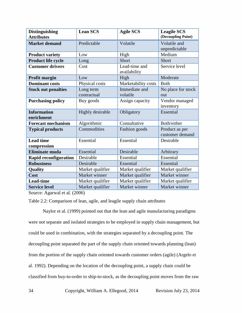
34 Copyright, William A. Ellegood, 2014 Revision July 23, 2014
Distinguishing
Attributes
Lean SCS Agile SCS Leagile SCS (Decoupling Point)
Market demand Predictable Volatile Volatile and
unpredictable
Product variety Low High Medium
Product life cycle Long Short Short
Customer drivers Cost Lead-time and
availability
Service level
Profit margin Low High Moderate
Dominant costs Physical costs Marketability costs Both
Stock out penalties Long term
contractual
Immediate and
volatile
No place for stock
out
Purchasing policy Buy goods Assign capacity Vendor managed
inventory
Information
enrichment
Highly desirable Obligatory Essential
Forecast mechanism Algorithmic Consultative Both/either
Typical products Commodities Fashion goods Product as per
customer demand
Lead time
compression
Essential Essential Desirable
Eliminate muda Essential Desirable Arbitrary
Rapid reconfiguration Desirable Essential Essential
Robustness Desirable Essential Essential
Quality Market qualifier Market qualifier Market qualifier
Cost Market winner Market qualifier Market winner
Lead-time Market qualifier Market qualifier Market qualifier
Service level Market qualifier Market winner Market winner
Source: Agarwal et al. (2006)
Table 2.2: Comparison of lean, agile, and leagile supply chain attributes
Naylor et al. (1999) pointed out that the lean and agile manufacturing paradigms
were not separate and isolated strategies to be employed in supply chain management, but
could be used in combination, with the strategies separated by a decoupling point. The
decoupling point separated the part of the supply chain oriented towards planning (lean)
from the portion of the supply chain oriented towards customer orders (agile) (Argelo et
al. 1992). Depending on the location of the decoupling point, a supply chain could be
classified from buy-to-order to ship-to-stock, as the decoupling point moves from the raw

Revision July 23, 2014 Copyright, William A. Ellegood, 2014 35
material supplier to the retailer. Naylor et al. (1999) provided a discussion of the
similarities and difference of lean and agile manufacturing paradigms, acknowledging
that with both a lean SCS and an agile SCS there was a necessity to compress lead times.
However, with a lean SCS the objective was cost minimization compared to an agile
SCS, where response time reduction was the primary objective. A supply chain with an
agile SCS focused on lead time compression in both information and material exchanges.
The paper demonstrated that a lean SCS and an agile SCS were not strategies that should
be viewed as only either/or, but together as a leagile SCS that could both reduce the total
supply chain cost relative to an agile SCS and increase responsiveness of the supply chain
to changes in demand relative to a lean SCS.
Mason-Jones et al. (2000a) presented three case studies to illustrate the
circumstances under which a lean SCS, an agile SCS, and a leagile SCS should be
implemented. The first case was of a United Kingdom manufacturer that employed a lean
global supply chain to export its products to the USA, Japan, Korea and Europe. With the
implementation of a distribution requirement planning system linked to the customers,
the firm was able to greatly improve their forecast accuracy. In addition, the company
implemented a kanban system for the production floor. The second case examined a
carpet manufacturer where the firm implemented parallel lean and agile supply chains,
where the lead time of the lean SCS was four weeks and the lead time of the agile SCS
was one week. The products assigned to the lean SCS included 90% of their product
offerings and accounted for 48% of total sales. The top 10% of their product offerings
accounted for 52% of total sales and were produced under an agile SCS. The third case
study was of a leagile SCS at an electronic product manufacturer where components were

36 Copyright, William A. Ellegood, 2014 Revision July 23, 2014
produced and purchased based on forecasted demand (lean SCS) and the final assembly
was scheduled based on actual orders (agile SCS). The case studies were used to
demonstrate that a one size fits all approach to SCS was incorrect and that the appropriate
SCS depended on the demand characteristics of the market.
Christopher and Towill (2001) discussed various approaches that a supply chain
could employ using both a lean and an agile SCS to satisfy customer demand. The article
described three approaches: Pareto, “base and surge”, and a de-coupling point. With the
Pareto approach the supply chain would utilize a lean SCS for the top 20% of products
that satisfy 80% of the demand and an agile SCS for the other 80% of products that
satisfy 20% of the demand. The “base and surge” approach was frequently utilized in the
fashion industry where a lean SCS was used to satisfy the portion of expected demand
that can be forecasted with a high level of confidence, the “base”, and an agile SCS was
used to satisfy the portion of demand that was difficult to forecast, the “surge”. The de-
coupling point approach was a supply chain where a lean SCS was used up to the de-
coupling point, and downstream of the de-coupling point an agile SCS was employed.
Towill and Christopher (2002) proposed a framework for firms to adopt both a lean SCS
and an agile SCS dependent upon time and space. The article presented three cases, with
each case demonstrating one of the strategies presented in Christopher and Towill (2001):
base and surge, Pareto, and decoupling.
Aitken et al. (2002) presented a case study of a United Kingdom lighting
company where several of their product families had become commodity products with
offshore competitors competing on price. The United Kingdom firm was unable to reduce
costs to a point that would allow them to compete on price, so they adopted an agile SCS

Revision July 23, 2014 Copyright, William A. Ellegood, 2014 37
to improve customer service. To achieve the new agile SCS, the United Kingdom lighting
company had to significantly reduce lead times. The firm’s products were segmented
based on a framework where the appropriate SCS was dependent upon the level of
product variety and demand predictability.
Stratton and Warburton (2003) examined how the supply chain strategies of lean
and agile could be integrated. The authors pointed out that many firms produced a variety
of products with different levels of demand uncertainty and that a one size fit all SCS was
not appropriate to satisfy customer expectations. Products could be separated into groups
based on space, “whole and its parts”, time, or condition to determine the appropriate
SCS for a product or a group of products. Separation in space was separating based on
different business environments, such as stable versus unstable demand. Separation of a
“whole and its parts” was separating the SCS about a decoupling point as in a leagile
SCS. Separation in time was adopting a “base and surge” strategy, where the stable
portion of demand was supplied by the lengthier lean SCS and the unstable portion was
supplied by the shorter agile SCS. Separation upon condition was separating on order
winning criteria, such as price (lean SCS) and delivery speed (agile SCS). A framework
for identifying the appropriate SCS based on product type (special or standard) and
demand uncertainty (volatile or stable) was presented where an agile SCS was indicated
when demand uncertainty was volatile and independent of the product type, and a lean
SCS was suggested for standard product type with low demand uncertainty (stable).
Naim and Gosling (2011) provided an examination and classification of the
citations of Naylor et al. (1999). Only one article reviewed explored the relationship
between SCS and PLC (Vonderembse et al. 2006). Overall the articles reviewed show

38 Copyright, William A. Ellegood, 2014 Revision July 23, 2014
strong support for a third SCS, leagile, which combined lean and agile strategies about a
decoupling point. Most articles also noted that a leagile SCS, like a lean SCS and an agile
SCS, was neither better nor worse than the other supply chain strategies and that the
appropriate SCS for a product was dependent on a combination of factors.
2.4 Product life cycle and supply chain strategy
The literature examining SCS over the PLC can be grouped into two categories:
(1) the SCS should change over the PLC as the demand characteristics of the product
change (Christopher and Towill, 2000; Childerhouse et al., 2002; Aitken et al., 2003;
Holstrom et al., 2006; Jeong, 2011); and (2) the SCS for a product should be determined
prior to market introduction and should not change over the PLC (Randall and Ulrich,
2001; Cigolini, 2004; Stradtler, 2005; Juttner et al., 2006; Vonderembse et al., 2006;
Seuring, 2009). As a product progresses through its PLC, the classification of the product
as innovative or functional may change. The classical PLC model has four stages:
introduction, growth, maturity, and decline (Cox, 1967). The introduction and growth
stages are characterized by demand instability and higher margin contribution compared
to the maturity stage, which is characterized by greater demand stability and lower
margin contribution (Rink and Swan, 1979).
A case study of a United Kingdom lighting manufacturer was presented in
Childerhouse et al. (2002) to evaluate the product classification system proposed in
Christopher and Towill (2000). The purpose of the system was to identify the appropriate
process by which demand information was conveyed to the manufacturing floor and the
coinciding demand chain strategy to be employed for a product as it moved through its
PLC. The acronym DMV3 was used to represent the parameters in the product
Revision July 23, 2014 Copyright, William A. Ellegood, 2014 39
classification system: duration of life cycle, time window for delivery, volume, variety,
and variability. The research considered a classical PLC, shown in Figure 1.2, with five
stages, where the maturity stage of Figure 1.2 was divided into two stages “maturity” and
“saturation”. The research identified the following supply chain strategies for a product
throughout its PLC: introduction stage – build to order, growth stage – MRP (agile),
maturity stage – Kanban (lean), saturation stage – packing center (leagile), and decline –
MRP (agile). The researchers found that by employing a different strategy at different
PLC stages, the organization was focused on the correct product “order winner”, service
level or cost, throughout the PLC. Aitken et al. (2003) provided an update to the case
study in Childerhouse (2002) which included a flow diagram of the decision process used
to determine when a product moved from stage to stage in its PLC.
A framework of supply chain management presented by Stadtler (2005) illustrated
that supply chain management was built on a foundation of business functional areas,
leading to the integration and coordination of supply chain partners to achieve a
competitive advantage. Supply chain partners entered into a partnership expecting the
relationship would result in a win-win situation over the life cycle of the product. With a
single SCS for a product over its life cycle there were periods where one partner may
achieve a financial benefit from another partner by utilizing a less than locally optimal
strategy for the greater good of the supply chain. For these instances the supply chain
should have methods to transfer or share the financial benefits between supply chain
partners.
The purpose of Holmstrom et al. (2006) was to better understand how demand
information could be used by organizations at different stages of the PLC. The

40 Copyright, William A. Ellegood, 2014 Revision July 23, 2014
researchers conducted a case study of a large manufacturer of durable consumer products.
During the period prior to product introduction, planning and forecasting based on
previous product launches was used to determine the production mix for the product.
During the introduction stage of the PLC, point-of-sale or channel inventory data should
be used to make adjustments to the product production mix. Once the product had
reached the maturity stage of its PLC, demand information should be used to drive
supply. During the decline phase, demand information should be used to develop plans to
consume current in-process inventory in order to minimize the cost associated with
obsolete inventory. The authors concluded that a supply chain should use demand
information differently at different stages of the PLC, similar to Childerhouse et al.
(2002).
Juttner et al. (2006) presented a case study to examine how the alignment of
demand chain strategy and market segment could increase value over the life-cycle of a
product. The case study considered a tobacco company that supplied the Eastern
European market with cigarettes. The research found when the tobacco company aligned
the manufacturing strategy of a product with that of the products market segment, value
to the consumer was increased. An agile SCS should be employed for products with a
large number of varieties and low volume, high value products, higher priced products,
and products with a high degree of customization, and a lean SCS should be employed
for products with a small number of varieties and high volume, low value products, and
products with a high degree of standardization.
Seuring (2009) described a conceptual model proposing that a product’s SCS was
dependent upon the stage of the PLC and whether the product was part of a new or

Revision July 23, 2014 Copyright, William A. Ellegood, 2014 41
established supply chain. The framework described the three stages of the PLC as product
design, production, and product return. The research supported the framework by
examining six previously published cases.
Jeong (2011) presented an analytical model to identify the optimal inventory
policy to minimize the total cost of deviations from targeted production rates and
inventory levels of a product where demand followed the growth-maturity PLC. The
growth-maturity PLC is similar to classical PLC; however, with the growth-maturity PLC
expected demand remains essentially constant once it reaches the point of peak demand
and there is no decline stage. The author considered a zero inventory policy and a
production smoothing policy. Under the zero inventory policy, the model provided a
function for the optimal time in the PLC to change from a make-to-stock to a make-to-
order policy to minimize total cost deviation. When considering a production smoothing
policy, the model provided the optimal production rate to minimize total cost deviation.
Hashemi et al. (2013) presented a structural equation model to examine the
impact product design and product demand complexity had on the level of supply chain
complexity. The paper discussed the model and the survey instrument only. The paper
provided a discussion of previous frameworks for SCS selection and divided the
characteristics considered into those that focused on demand aspects and those that
focused on product design aspects. The purpose of the model was to provide insight to
the extent to which product design and demand uncertainty impact supply chain strategy.
When considering the literature that recommended the SCS of a product should
change during the PLC, a more accurate interpretation of the conclusions would be the

42 Copyright, William A. Ellegood, 2014 Revision July 23, 2014
method employed by the firm to convey demand information to the operations
department should change during the PLC. The literature concluding the SCS of a
product should be determined prior to market introduction considered supply chain
management in a broader sense as the planning and management of information and
material flow between organizations from raw materials to the end consumer. The
concept that the SCS of a product should be determined prior to market introduction is an
extension of the engineering principle, “design for manufacturing”, where consideration
to the ease of manufacturability of a product is evaluated during the design stage of the
product. The literature supports the concept of “design for SCM”, where the SCS of a
product is considered during the design stage of the product to improve the flow of
material and information throughout the supply chain over the life-cycle of the product.
2.5 Supply chain strategy selection and improvement
Several articles have used quantitative methods (e.g. mathematical programming,
simulation modeling, etc.) to determine the combination of strategies that improved
supply chain performance the most. Measures of supply chain performance that have
been examined include optimizing multiple objectives considering profit, delivery lead
time and promptness (Li and O’Brien, 1999; Li and O’Brien, 2001); delivery reliability,
flexibility and responsiveness, cost, and assets (Wang et al., 2004); maximizing market
responsiveness (Agarwal et al., 2006); customer service and cost (Goldsby et al., 2006);
and minimizing the sum of supply chain and emissions costs (Besbes et al., 2012).
Li and O’Brien (1999) presented a multistage dynamic decision model to
determine the combination of operational strategies to minimize the total dissatisfaction
level of a three echelon supply chain. The dissatisfaction level was the weighted sum of
Revision July 23, 2014 Copyright, William A. Ellegood, 2014 43
the gaps between realized and target performance in four areas: profit, lead time, delivery
promptness, and waste elimination. The model considered the operational strategies of
make-to-order (lean SCS), make-from-stock (agile SCS), and make-to-stock (leagile
SCS). The model was evaluated using an artificial data set. The researchers found that
when the ordering lead time was shorter than the delivery lead time, an inventory buffer
was needed. The location of the inventory buffer in the supply chain was modeled as a
decoupling point between the supply chain strategies. The research demonstrated that for
the scenarios presented, a combination of SCS minimized total dissatisfaction level.
Li and O’Brien (2001) presented a multiple objective optimization model to
determine the SCS which resulted in the best performance when considering demand
uncertainty and value-added capacity. The researchers considered three strategies and
related each strategy to the strategies presented in Fisher (1997): manufacturing-to-order
or MTO (lean SCS) described as physically efficient, manufacturing-from-stock or MFS
(agile SCS) described as market responsive, and manufacturing-to-stock or MTS (leagile
SCS) described as physically responsive. Supply chain performance was measured as the
summation of the weighted gaps in achieving the objectives of three areas: profit,
delivery lead time, and delivery promptness, with weights of 0.35, 0.35 and 0.30,
respectively. Demand uncertainty was a factor used to determine the expected delivery
delay and would have been better defined as supply uncertainty. The MTO strategy was
modeled with no supply uncertainty in the supply chain. The MFS strategy was modeled
with supply uncertainty only at the supplier and the MTS strategy was modeled with
supply uncertainty at both the supplier and the production facility. Value-added capacity
was the ratio of materials cost to finished product price. The authors considered fifteen

44 Copyright, William A. Ellegood, 2014 Revision July 23, 2014
combinations of supplier and production demand uncertainty at five levels of value-added
capacity. The research demonstrated that the SCS which resulted in the best performance
was dependent on the supplier uncertainty, production facility uncertainty and value-
added capacity.
De Treville et al. (2004) drew upon previous published case studies to assert that
a firm should focus on lead time reduction before information sharing to improve the
responsiveness of a supply chain. The authors provided several propositions in support of
their position. First was that demand information received after the start of production
adds to transaction uncertainty. Second was that an improvement that reduced lead time
was more likely to reduce transaction uncertainty than an improvement in information
sharing. Third was that focusing on one area was more likely to reduce transaction
uncertainty than focusing on both lead time reduction and information sharing
simultaneously.
Wang et al. (2004) blended Huang et al. (2002) and Fisher (1997) with the SCOR
framework developed by Supply Chain Council (SCC, 1999) in a multi-criteria decision-
making model to assist practitioners with supplier selection dependent on product type
and the objective of the supply chain. The researchers developed an analytic hierarchy
process model based on the four categories of the SCOR framework: delivery reliability,
flexibility and responsiveness, cost, and assets. The model was evaluated using artificial
data for three products and three potential suppliers for each product. The evaluation of
the model demonstrated the effectiveness of the SCOR framework in assisting
practitioners with supplier selection: the supplier employing a lean SCS was selected for

Revision July 23, 2014 Copyright, William A. Ellegood, 2014 45
the functional product, the supplier with a leagile SCS was selected for the hybrid
product, and the supplier with an agile SCS was selected for the innovative product.
The framework presented in Agarwal et al. (2006) assisted practitioners in
determining the best SCS when performance of a supply chain was measured by its
market responsiveness. The analytic network process developed by the authors
considered supply chain attributes from four areas: market sensitiveness, information
drivers, process integration, and flexibility. A group of experts were consulted to
establish the relative importance between the attributes. Sensitivity analysis was
completed varying the relative importance of the attributes, from 1/9 to 9, with all other
terms held constant. The sensitivity analysis of lead time relative to cost showed that
when greater importance was placed on cost than lead time, a lean SCS was appropriate.
When the importance of cost and lead time were approximately equal then a leagile SCS
was recommended, and when a greater importance was place on lead time compared to
cost, then an agile SCS should be adopted. The research showed that even when market
responsiveness was the objective of the supply chain, there were combinations of supply
chain attributes and firm’s objectives which could drive a firm to employ a SCS other
than an agile SCS.
Goldsby et al. (2006) presented a simulation model of a three echelon supply
chain to examine the customer service and cost impact of adopting an agile, a leagile, or a
lean SCS. The supply chain consisted of a manufacturer, one or two distribution centers
depending upon the strategy employed, and seven customers. The agile SCS was
modeled with no finished goods inventory located at the distribution center or the
manufacturer, one distribution center to serve all seven customers, and the

46 Copyright, William A. Ellegood, 2014 Revision July 23, 2014
manufacturer’s operational strategy was build-to-order. The leagile SCS was modeled
with partially completed products inventoried at the two distribution centers and the
manufacturer produced partially completed product based on forecasted demand. The
lean SCS was modeled with finished inventory at the two distribution centers and the
manufacturer produced completed product based on forecasted demand. The simulation
showed that a lean SCS resulted in a higher level of customer service and had more total
inventory in the supply chain than both the leagile SCS and agile SCS. As a result of how
the agile SCS was modeled, with no finished goods inventory, sensitivity analysis
showed that as the value of finished goods increased or as holding cost increased, an agile
SCS resulted in a lower total supply chain cost.
The purpose of Hilletofth (2009) was to examine how firms employed operational
strategies to develop differentiating SCS. The research presented case studies of a
Swedish firm from the telecommunication industry and a Swedish firm from the
appliance industry. The operational strategies of make-to-stock (MTS), deliver-to-order
(DTO), assemble-to-order (ATO), sourcing-to-order (STO), and make-to-order (MTO)
were considered. The article concluded the first step for identifying the appropriate SCS
was to develop a product segmentation model based on geography, product type, and
customer type. Then the appropriate combination of operational strategies should be
selected by the firm to achieve a differentiated supply chain based on the firm’s
understanding of the market and their ability to serve the market.
Besbes et al. (2012) presented a two phase modeling approach for supply chain
member selection over the life-cycle of a product. The first phased included an analytic
hierarchy process to determine the efficiency score of potential suppliers, production

Revision July 23, 2014 Copyright, William A. Ellegood, 2014 47
facilities, and distributors. The second phase was a multiple objective mathematical
model to select the suppliers, producers, and distributors for each time period with an
objective to minimize the summation of supply chain costs and carbon dioxide emission
costs for all time periods. An example based on an actual supply chain was presented.
The authors found when the supply chain utilized a different combination of suppliers,
producers, and distributors for the introduction stage than for the maturity stage of the
life-cycle, the total supply chain and carbon dioxide emission costs could be minimized.
The article did not discuss the supply chain strategy of the various potential supply chain
members.
2.6 Analytical models for supply chain strategy selection
Researchers have utilized analytical models to examine many areas of supply
chain management. This section provides a brief survey of articles that consider
analytical modeling to identify the appropriate SCS.
Herer et al. (2002) demonstrated with an analytical model how transshipment
could be used as an inexpensive strategy to achieve a leagile supply chain. The research
demonstrated mathematically that with transshipment a distribution network could reduce
costs and improve service levels when compared to a distribution network without
transshipment.
Kim and Ha (2003) developed an analytical model to determine the order quantity
and the number of shipments for a single setup multiple delivery problem. The two
echelon supply chain model included setup and inventory holding cost parameters for the
seller, and ordering, inventory holding, and transportation cost parameters for the buyer.

48 Copyright, William A. Ellegood, 2014 Revision July 23, 2014
A possible application for the model was for Kanban systems, where the number of
shipments was the number of Kanban cards in the system.
Gupta and Benjaafar (2004) described a two stage analytical model of a make-to-
order, make-to-stock, and decoupling point strategy to minimize the total inventory
holding and backorder costs. A key parameter of the model was the capacity utilization of
each stage. The analysis showed that when the capacity utilization of either stage was
high, a make-to-stock strategy was more effective than a decoupling point strategy. When
a decoupling strategy was employed, the strategy was more effective when those
operations with higher capacity utilization were moved to the make-to-stock side of the
supply chain.
Ahn and Kaminsky (2005) developed an analytical model to evaluate production
and distribution policies of a two stage stochastic push-pull supply chain with an
objective of total cost minimization. The supply chain was modeled so that the supply
side followed a make-to-stock strategy and the demand side followed a make-to-order
strategy. The model included costs associated with production, transportation, and
inventory holding. The model assumed demand occurred according to a Poisson process.
The authors derived a heuristic function for the economic order quantity that minimized
total cost of the supply chain. The robustness of the heuristic was evaluated with a wide
variety of parameters and the heuristic was found to be within 2% of the optimal solution.
Gupta and Benjaafar (2004) and Ahn and Kaminsky (2005) utilized analytical
modeling to determine the best location of the decoupling point. Ernst and Kamrad
(2000) demonstrated for supply chains with two customers a lean SCS was appropriate

Revision July 23, 2014 Copyright, William A. Ellegood, 2014 49
when the service level and demand uncertainty of the customers were similar, and an
agile SCS should be employed when service levels and demand uncertainty of the
customers differed greatly. Jeong (2011) presented an analytical model to identify the
optimal inventory policy for a product where expected demand followed the growth-
maturity PLC.
There has been limited research employing analytical modeling to examine SCS
selection and the following gaps in the literature will be examined by this dissertation: (1)
when a “misalignment” of SCS and product type might result in the best supply chain
performance; (2) the appropriate SCS for a wide variety of supply chain structures and
product/supply chain characteristics; and (3) the appropriate SCS over the life-cycle of a
product.
2.7 Net present value and supply chain management
The net present value of supply chain costs should be determined to evaluate the
value of the SCS over time (Kilbi et al., 2010). Guillen et al. (2005) developed a multiple
objective stochastic model to determine the best supply chain network when the multiple
objectives listed previously were considered. When designing a supply chain network
under uncertainty to maximize expected profit, achieve a minimum service level, or
minimize risk (the probability that expected profit falls below a targeted profit level)
there are a large number of factors to consider. The first objective was to maximize the
net present value of expect profit, where the net present value of costs to satisfy the
demand and the revenue from the demand were incurred during the time period the
demand was realized. A hypothetical case study was used to evaluate the model and
identify the Pareto frontiers between the objectives.
50 Copyright, William A. Ellegood, 2014 Revision July 23, 2014
To evaluate the cash flow impact of information sharing, Naim (2006) developed
a net present value (NPV) spreadsheet simulation model. The author pointed out that
although the literature had presented a number of measurements for supply chain
performance, ultimately supply chain management decisions had monetary consequences
and should incorporate cash flow analysis. The research included a cash flow equation as
a function of time, where the profitability of the supply chain equaled the net present
value of product revenue less the summation of variable cost and inventory holding cost;
ordering cost was not considered. Three supply chains were considered to evaluate the
impact of information sharing on cash flow: traditional – no information sharing, vendor
managed inventory – the first two echelons had actual demand information, and e-
commerce point of sale (EPOS) – demand information was shared with all echelons.
Three ceteris paribus simulations were considered where each of the following variables
was changed holding all others were constant: variable cost, holding cost, and cost of
capital. Under all three simulations, the EPOS supply chain was superior to the other two
supply chain strategies for all variable values considered, demonstrating the value of
information sharing.
Franca et al. (2010) presented a multiple objective stochastic model which
included the net present value of a supply chain’s cash flows. The objective of the first
stage of the model was to maximize expected profit and the objective of the second stage
was to minimize supplier defects. The model did not consider lead time; therefore, all
costs incurred to supply the product were incurred during the same time period as the
demand. The model was evaluated using simulated data and the results showed that
quality improvements had a positive impact on profit except when the defect rate was

Revision July 23, 2014 Copyright, William A. Ellegood, 2014 51
very high (greater than 100,000 per million). The Pareto frontier for a supply chain could
provide critical information during supplier selection, as all suppliers with defect rates
greater than this frontier should not be considered.
Disney et al. (2013) reformulated the classic economic production quantity (EPQ)
model to incorporate NPV. When EPQ was evaluated considering the NPV of cash flow,
no closed form solution could be determined for the optimal production quantity. The
researchers used a Taylor Series to formulate an approximate total cost function and from
the approximate total cost function the optimal production quantity could be determined.
Scenario analysis was done to demonstrate that the percentage error of the approximate
total cost function was within 2% of optimal cost and the accuracy of the approximate
total cost function improved as the difference between the demand and production rates
increased.
There has been a growing recognition in supply chain management literature that
a more accurate valuation of supply chain costs should consider the timing of financial
flows. Research that examines supply chain strategy selection and the NPV of financial
flow is very limited. This dissertation addresses this gap in the literature.
2.8 Summary
The Fisher Model identified two supply chain strategies and two product types,
where the SCS and product type should be aligned for SCM to be successful. Most
researchers considered only two or three supply chain strategies to assess when each was
the best. Many of the SCS frameworks that extended the Fisher Model acknowledge that
there are at least three classifications of supply chain strategies: lean SCS, leagile SCS,

52 Copyright, William A. Ellegood, 2014 Revision July 23, 2014
and agile SCS. Three researchers presented frameworks that considered four supply chain
strategies (Pagh and Cooper, 1998; Ernst and Kamrad, 2000; Lee, 2002); however, none
consider the agilean SCS as described in this research. The agilean SCS, where the
supply side employs a responsive strategy and the demand side employs a cost
minimization strategy, can be an effective strategy to shorten the overall length of the
supply chain while still benefiting from the cost advantage of the lean strategy when the
majority of a product’s costs are incurred late in the supply chain.
Many of the articles reviewed found a statistically significant relationship
between supply chain performance and the alignment between SCS and demand
characteristics. However, other researchers found that this was not true in all cases. This
lack of generalizability of the alignment between SCS and demand characteristics is an
area that this dissertation examines to provide managerial insights regarding the scenarios
in which a misalignment of SCS and product type might minimize total NPV supply
chain cost. There is a significant gap in the literature concerning the use of analytical
models to assist practitioners with determining the appropriate SCS. This gap in the
literature is the second area this dissertation examines by presenting a NPV analytical
model of a multi-echelon supply chain to evaluate all four possible supply chain
strategies, and the sensitivity of each SCS to operating and demand characteristics.
The most current literature examining supply chain strategies and product life-
cycles suggested that the SCS of a product should be determined prior to market
introduction during the design phase of the product. However, no research has provided a
rigorous examination the circumstances when each type of SCS minimizes total cost over
the entire PLC. In addition, no research has examined how a change in the length of the

Revision July 23, 2014 Copyright, William A. Ellegood, 2014 53
PLC or the total expected demand impacts the SCS that minimizes total cost, nor has the
research examined how the SCS of a product might best evolve during a PLC to
minimize the impact to total cost. The third focal area of this dissertation addresses these
gaps: (1) identifies the SCS that minimizes total NPV supply chain cost over the entire
PLC, (2) provides managerial insight on how a change in the PLC length or the total
expected demand might impact the SCS that minimizes total NPV supply chain cost over
the entire PLC, and (3) presents a strategy to best evolve a supply chain from agile to lean
to minimize the impact to total NPV supply chain cost over the entire PLC.

54 Copyright, William A. Ellegood, 2014 Revision July 23, 2014
3. Analytical model
Analytical modeling is a valuable technique to examine the overall performance
of a supply chain, providing strategic managerial insights as to how an objective (e.g.
minimize total cost) is impacted as parameters and/or the relationship of parameters are
varied. The benefits of analytical modeling can be furthered when probabilistic and
uncertain attributes are incorporated into the model. A difficulty of analytical modeling is
to describe the system in sufficient detail that useful results can be derived, but not in so
much detail that managerial insights are lost in model complexity. A description of the
notation used in this research is presented in Table 3.1.
3.1 Notation
Parameter Description
( ) General Total Cost function
( ) Total Cost function when expected demand and demand forecast error are
constant
( ) Total Cost function when expected demand is a linear function of time and
demand forecast error is constant
( ) Total Cost function when expected demand mimics classical PLC and
demand forecast error is an exponential decay function with respect to time
( ) Agile SCS Total Cost function
( ) Agilean SCS Total Cost function
( ) Leagile SCS Total Cost function
( ) Lean SCS Total Cost function
Total net present value of supply side material cost function
Total net present value of supply side inventory cost function
Total net present value of supply side ordering cost function
Total net present value of demand side production cost function
Total net present value of demand side inventory cost function
Total net present value of demand side ordering cost function
Total expected demand over the PLC
Purchased material cost per unit for supply chain strategy
Lead time for supply chain strategy and supply chain side
Manufacturing cost per unit for supply chain strategy
Number of orders for supply chain side
Number of orders for supply chain side of epoch
Revision July 23, 2014 Copyright, William A. Ellegood, 2014 55
Optimal number of orders for supply chain side
Order processing cost for supply chain side
( ) Total net present value supply chain ordering cost for ( ) ( ) Total net present value supply chain production cost for ( ) Number of epochs for the PLC
Relative manufacturing cost – the percentage of manufacturing costs to total
production costs for a lean SCS
Ratio of manufacturing cost to purchased material cost – ratio of demand
side manufacturing cost to supply side purchased material cost of a lean SCS
Duration in days of the forecast period
Duration in days of the PLC
Length in days of each epoch
Net present value for a series of costs
Confidence interval factor for the service level for supply chain strategy
and supply chain side
Constant terms for the PLC expected demand function
( ) Expected demand as a continuous function of time
Expected discrete demand for day
( ) Actual demand as a continuous function of time
Actual discrete demand for day
Average demand for the forecast period [ ] ( ) Demand forecast error as a continuous function of time
Demand forecast error for day
Cost of capital
Index of time in days
Last day of order period for supply chain side
Last day of order period for supply chain side of epoch
Index of epochs
Index of order periods for supply chain side from 1 to
Index of order periods for supply chain side from 1 to of epoch
Continuous time
Decay factor for demand forecast error
Standard deviation of expected demand for day
Standard deviation of the cumulative distribution function for order
Slope of the expected demand function over the length of the forecast period
Ratio of agile SCS purchased material unit cost to lean SCS purchased
material unit cost
Ratio of agile SCS manufacturing unit cost to lean SCS manufacturing unit
cost
Half the probability range that will be within of
Attributes describing the number of orders and the costs per order
Attributes describing demand and the forecast period
Attributes describing the SCS
Subscript Description

56 Copyright, William A. Ellegood, 2014 Revision July 23, 2014
A parameter associated with the supply side of the supply chain
A parameter associated with the demand side of the supply chain
An agile strategy parameter
A lean strategy parameter
A parameter dependent on the strategy type, ( or )
A parameter dependent on the side of the supply chain, ( or )
Table 3.1: Parameters and coinciding description
The general total NPV supply chain cost model (Total Cost) is not specific to a
particular SCS and is denoted without a subscript. When the model is specific to an agile
SCS, an agilean SCS, a leagile SCS, or a lean SCS, the subscripts or are
used to denote the SCS, respectively. A two letter subscript is used to identify the SCS of
each side of the supply chain, with the supply side strategy denoted by the first subscript
and the demand side strategy signified by the second subscript. The subscript denotes a
parameter that is dependent on the strategy type, so when the is replaced by , then an
agile strategy or parameter is employed and when it is replaced by a , then a lean
strategy or parameter is adopted. The subscript signifies a parameter dependent on the
side of the supply chain: when is replaced by , it denotes a parameter associated with
the supply side of the supply chain, and when the is replaced by it signifies a
parameter associated with the demand side of the supply chain.
3.2 Model description
The analytical cost model presented in this research is the summation of supply
side and demand side NPV supply chain costs of a three echelon supply chain (supplier,
manufacturer, and customer) with a decoupling point at the manufacturer and two
inventory points as presented in Figure 3.1.
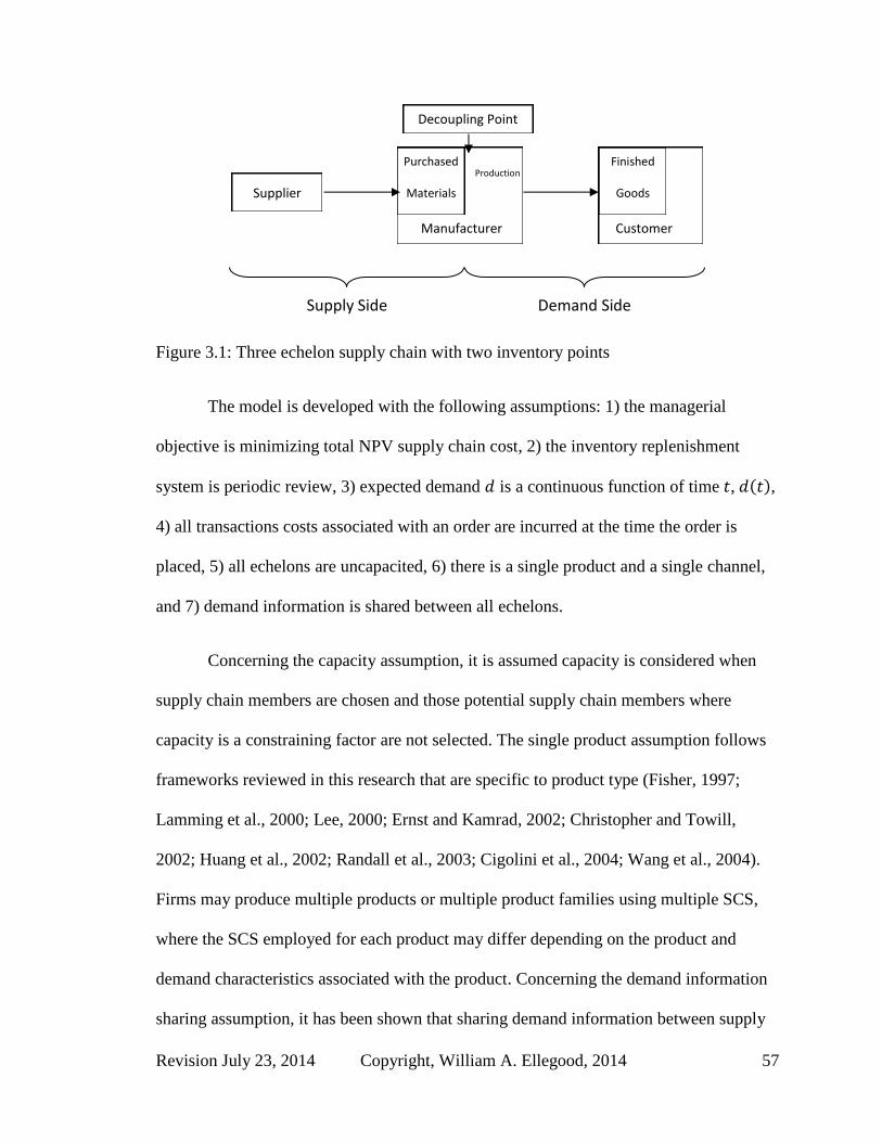
Revision July 23, 2014 Copyright, William A. Ellegood, 2014 57
Figure 3.1: Three echelon supply chain with two inventory points
The model is developed with the following assumptions: 1) the managerial
objective is minimizing total NPV supply chain cost, 2) the inventory replenishment
system is periodic review, 3) expected demand is a continuous function of time , ( ),
4) all transactions costs associated with an order are incurred at the time the order is
placed, 5) all echelons are uncapacited, 6) there is a single product and a single channel,
and 7) demand information is shared between all echelons.
Concerning the capacity assumption, it is assumed capacity is considered when
supply chain members are chosen and those potential supply chain members where
capacity is a constraining factor are not selected. The single product assumption follows
frameworks reviewed in this research that are specific to product type (Fisher, 1997;
Lamming et al., 2000; Lee, 2000; Ernst and Kamrad, 2002; Christopher and Towill,
2002; Huang et al., 2002; Randall et al., 2003; Cigolini et al., 2004; Wang et al., 2004).
Firms may produce multiple products or multiple product families using multiple SCS,
where the SCS employed for each product may differ depending on the product and
demand characteristics associated with the product. Concerning the demand information
sharing assumption, it has been shown that sharing demand information between supply
Production
Manufacturer
Supplier
Customer
Purchased
Materials
Inventory
Finished
Goods
Inventory
Decoupling Point
Supply Side Demand Side

58 Copyright, William A. Ellegood, 2014 Revision July 23, 2014
chain members improves the performance of the supply chain (Gavirneni et al., 1999;
Kim, 2000; Lee et al., 2000; Raghunathan, 2001; Aviv, 2001; Xu et al., 2001;
Thonemann, 2002; Naim, 2006; Ouyang, 2007). However, the purpose of this research is
not to determine the impact of demand information sharing on the appropriate SCS for a
product. The material flow of the supply chain is from the supplier to the manufacturer;
the manufacturer then transforms a unit of purchased material into a unit of finished
goods, and the unit of finished goods is shipped from the manufacturer to the customer.
There are a number of objectives that a firm may adopt for evaluating the
performance of a SCS, including but not limited to: maximize profit (Guillen et al.,
2005;), minimize total cost (Kim and Ha, 2003; Ahn and Kaminsky, 2005; Naim, 2006),
maximize responsiveness (Agarwal et al., 2006), minimize inventory cost (Gupta and
Benjaafar, 2004), and minimize cost deviations (Jeong, 2011). Further, some research
considered multiple objectives (Li and O’Brien, 1999; Li and O’Brien, 2001; Herer et al.,
2002; Franca et al., 2010). Ultimately the adoption of a SCS has monetary consequences
(Naim, 2006); therefore, this research focuses on the strategic objective of total NPV
supply chain cost minimization.
The supply side costs include the purchased material unit cost and order
processing cost . The demand side costs are the manufacturing unit cost and order
processing cost . It is assumed that the supply chain members use either a traditional
cost accounting system or an activity based cost accounting system, as the model will
work with either cost accounting system. With a traditional cost accounting system, all
overhead costs are allocated per unit based on expected demand and either labor hours or
machine hours required per unit (Lin et al., 2001). With an activity based cost accounting

Revision July 23, 2014 Copyright, William A. Ellegood, 2014 59
system all overhead costs are traced to a product and are considered variable costs (Lin et
al., 2001). With a traditional cost accounting system those costs typically associated with
inventory holding cost are accounted for in the unit cost of the product (Grubbstrom,
1980).
The purchased material unit cost is defined as all costs, including allocated
overhead, incurred by the supply chain for the supplier to produce a unit of purchased
material and transport it to the manufacturer, excluding ordering costs. The supply side
ordering cost includes all costs incurred by the supply chain for each order placed by
the manufacturer to the supplier (e.g. order processing, machine setup, etc.), except for
transportation cost which is included in . Similarly, manufacturing unit cost is
defined as all costs, including allocated overhead, incurred by the supply chain for the
manufacturer to transform a unit of purchased material into a unit of finished goods and
transport it to the customer, excluding ordering costs. The demand side ordering cost
includes all costs incurred by the supply chain for each order placed by the customer to
the manufacturer (e.g. order processing, machine setup, etc.), except for transportation
cost which is included in . With transportation cost included in the purchased material
and manufacturing cost parameters, these parameters denote the delivered or landed cost
per unit for each side of the supply chain.
The model considers a forecast period from time to , where is a
positive integer that defines the length of the forecast period in days. Continuous time is
discretized such that is an integer [ ] reflecting one day of time. The model is
developed for firms that employ a periodic review replenishment system. When a firm
employs a periodic review replenishment system, the customer places orders to the
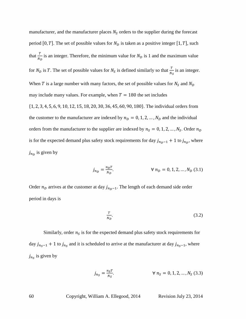
60 Copyright, William A. Ellegood, 2014 Revision July 23, 2014
manufacturer, and the manufacturer places orders to the supplier during the forecast
period [ ]. The set of possible values for is taken as a positive integer [ ], such
that
is an integer. Therefore, the minimum value for is 1 and the maximum value
for is . The set of possible values for is defined similarly so that
is an integer.
When is a large number with many factors, the set of possible values for and
may include many values. For example, when the set includes
{ }. The individual orders from
the customer to the manufacturer are indexed by and the individual
orders from the manufacturer to the supplier are indexed by . Order
is for the expected demand plus safety stock requirements for day to , where
is given by
. (3.1)
Order arrives at the customer at day . The length of each demand side order
period in days is
. (3.2)
Similarly, order is for the expected demand plus safety stock requirements for
day to and it is scheduled to arrive at the manufacturer at day , where
is given by
. (3.3)

Revision July 23, 2014 Copyright, William A. Ellegood, 2014 61
The length of each supply side order period in days is
. (3.4)
The purpose of the model is to capture the supply chain costs of a three echelon
supply chain over a forecast period [ ]. Expected demand can be viewed as a
continuous function of time ( ). Actual demand ( ) is assumed to be normally
distributed about expected demand. The continuous expected demand and actual demand
are discretized on a daily basis using equations (3.5) and (3.6), respectively.
∫ ( )
(3.5)
∫ ( )
(3.6)
The total expected demand for order period is
∑
∑
( )
. (3.7)
The total expected demand for all orders from the customer to the
manufacturer during the forecast period [ ] is
∑ ∑
( )
∑
. (3.8)
The total expected demand for all orders from the manufacturer to the supplier
during the forecast period [ ] is

62 Copyright, William A. Ellegood, 2014 Revision July 23, 2014
∑ ∑
( )
∑
. (3.9)
In this model, all transaction costs are assumed to be incurred at the time the order
is placed, which is a reasonable assumption under most operational strategies with the
exceptions of build-to-order and engineer-to-order. The research setting is where there is
expected demand and it is reasonable to assume that at least some inventory exists in raw
materials, work-in-process, and/or finished goods. Therefore, a portion, if not all, of the
costs associated with fulfilling the order has already been realized. The demand side lead
time, , is the response time in days that the manufacturer requires to deliver an order
to the customer and is dependent upon the demand side strategy employed. The time that
the manufacturer receives order is equal to the scheduled delivery time minus
the demand side lead time, . Therefore, the demand side costs for order are
incurred at time
. (3.10)
This may be negative, which simply implies the manufacturer receives the order prior to
the start of the forecast period.
The supply side lead time, , is the response time in days that the supplier
requires to deliver an order to the manufacturer and is dependent upon the supply side
strategy adopted. The time that the supplier receives order is equal to the scheduled
delivery time minus the summation of the demand side lead time, , and the
supply side lead time, . Therefore, the supply side costs for order are incurred at
time

Revision July 23, 2014 Copyright, William A. Ellegood, 2014 63
. (3.11)
This may be negative, which simply implies the supplier receives the order prior to the
start of the forecast period.
Figure 3.2 illustrates the point in time when costs are incurred by the
manufacturer and the supplier relative to order delivery time. This illustration
assumes . In this illustration the manufacturer
receives order 1 at time -2 and order 2 at time 3, while the supplier receives order 1 at
time -5 and order 2 at time zero.
Figure 3.2: Timing of manufacturer and supplier costs relative to order delivery time
The demand side cost for order includes the cost to manufacture and deliver
the order quantity to the customer (based on the manufacturing cost for the demand side
SCS, ), plus the order processing cost . The supply side cost for order includes
the purchased material cost and the cost to deliver the order quantity to the manufacturer
(based on the purchased material cost for the supply side SCS, ), plus the order
processing cost .
Cost
Cost
Customer
Manufacturer
Supplier
j
j
j
T
T
T 0
First order demand
Manufacturer receives first order
Supplier receives first order
Second order demand
Manufacturer receives second order
Supplier receives second order

64 Copyright, William A. Ellegood, 2014 Revision July 23, 2014
Fisher (1997) indicated the average forecast error of an innovative product is
greater than 40% and the average forecast error for a functional product is 10% or less.
However, the article did not provide a clear definition of average forecast error, a
discussion of forecast error distribution, nor the length of time for which the average
forecast error is calculated. Therefore, for this research demand forecast error at day is
assumed to be the absolute value of the difference between the expected demand, , and
the realized demand, , divided by ,
| |
. (3.12)
Although there are a number reasons for a forecast to be inaccurate, such as the
forecast method, the ability of the forecaster, external factors, and demand variability,
this research assumes that demand forecast error is the result of demand variability and
that can be approximated by a normal distribution about with a variance of :
[ ].
In this research the expected demand forecast error value is the percentage of
expected demand that defines a range that provides a 0.50 probability that the actual
realized demand will be within of the expected demand at time , as shown in Figure
3.3.
( ( ) ( )) . (3.13)

Revision July 23, 2014 Copyright, William A. Ellegood, 2014 65
Figure 3.3: Actual demand normally distributed about expected demand
From equation 3.13, the probability that is between and ( ) is 0.25.
Therefore, the standard deviation of actual demand can be determined by solving the
following equality,
,
. (3.14)
Other definitions of forecast error where is the probability that actual demand differs
from expected demand by no more than can be calculated using
. (3.15)
The service level of a supply chain side is dependent upon the supply chain
strategy for that side, denoted by . The safety stock inventory level of each order
period on either side of the supply chain depends on the service level associated with the

66 Copyright, William A. Ellegood, 2014 Revision July 23, 2014
strategy employed for that side of the supply chain, denoted by either or , and
the standard deviation of the cumulative distribution function (CDF) of demand for the
order period , and
. It is assumed that the demands are mutually
independent. The standard deviation of the CDF for an order period is equal to the square
root of the summation of the expected demand variances during the entire order period,
√∑
. (3.16)
Therefore, the safety stock inventory levels for each order period, , are
(3.17)
and
. (3.18)
The model assumes the initial safety stock inventory is zero for both sides of the
supply chain, given by
. (3.19)
A portion of each order is for the change in safety stock inventory level. The
change in safety stock inventory level from the previous order period to the next order
period for the demand side and the supply side are determined as follows:
[ ( )] (3.20)
and

Revision July 23, 2014 Copyright, William A. Ellegood, 2014 67
[ ( )]. (3.21)
When there is only a single order placed for the entire forecast period;
therefore, the total safety stock inventory requirement for the forecast period [ ] for
the demand side and supply side is
√∑
. (3.22)
To accurately assess the cost of a SCS the net present value (NPV), , of supply
chain costs should be determined (Kilbi et al., 2010). The net present value for a series of
costs, , (note: denotes a generic cost term and does not represent a
specific attribute) where cost occurs at day , and where is the cost of capital per
day is
∑ (3.23)
The general analytical model used in this research consists of the NPV of six cost
component functions: three to determine the total supply side cost and three to determine
the total demand side cost. The six component functions and a description of each
function are given in Table 3.2.

68 Copyright, William A. Ellegood, 2014 Revision July 23, 2014
Equations Function and description
3.7, 3.11,
3.23 [∑ (∑
) ( )
]
Total expected supply side NPV purchased material cost for the forecast
period [ ] for supply side SCS .
3.11, 3.21,
3.23 [∑ (
( )) ( )
]
Total expected supply side NPV purchased material safety stock inventory
cost for the forecast period [ ] for supply side SCS .
3.11, 3.23 ∑ ( )
Supply side NPV order processing cost for the forecast period [ ] for
supply side SCS .
3.7, 3.10,
3.23 [∑ (∑
) ( )
]
Total expected demand side NPV manufacturing cost for the forecast
period [ ] for demand side SCS .
3.10, 3.20,
3.23 [∑ (
( )) ( )
]
Total expected demand side NPV finished goods safety stock inventory cost
for the forecast period [ ] for demand side SCS .
3.10, 3.23
∑ ( )
Demand side NPV order processing cost for the forecast period [ ] for
demand side SCS .
Table 3.2: Six cost component functions for the Total Cost
3.3 Model construction
The general analytical model for the Total Cost of a three echelon supply chain
can be written as ( ), a function of sets of parameters that describe (i) the
ordering activities , (ii) the aspects of demand , (iii) the SCS , and (iv) the cost of
capital. The set includes those attributes that describe the number of orders and the cost
per order: the number of supply side orders ; the number of demand side orders ; the
supply side cost per order ; and the demand side cost per order . Thus
[ ]. The set includes those attributes that describe expected demand during
the forecast period: expected demand ; standard deviation of the CDF, and
, as
determined from the demand forecast error , and the standard deviation of demand ;

Revision July 23, 2014 Copyright, William A. Ellegood, 2014 69
and the length of the forecast period . Thus [
].The set
includes those attributes that describe the SCS: purchased material unit cost ;
manufacturing unit cost ; supply side lead time ; demand side lead time ;
supply side service level ; and demand side service level . Thus
[ ]. The Total Cost also depends on the cost of capital, . The
cost of capital is more than the time value of money; it is also an implicit measurement of
the risk associated with holding inventory. The risk of holding inventory is greater when
the time value of money increases and when there is increased risk of spoilage or
obsolescence associated with the product.
The general analytical model for the Total Cost of a three echelon supply chain is
the sum of the six component functions presented in Table 3.2,
( ) (3.24)
and in its expanded form
( ) [∑ (∑
) ( )
] [∑ (
( )) ( )] ∑
( )
[∑ (∑
) ( )
]
[∑ ( ( ))
( ) ] ∑ ( )
. (3.25)

70 Copyright, William A. Ellegood, 2014 Revision July 23, 2014
Simplification of equation (3.24) by factoring out common terms results in
( )
( ) [∑ ( {(∑
) (
( ))} ) ( ) ]
( ) [∑ ( {(∑
) (
( ))} ) ( )].
(3.26)
3.4 Supply chain strategy model construction
The four supply chain strategies in this research result from combining a lean and
an agile strategy for the supply and demand side of the supply chain. Parameter values for
the model were determined by mapping the cost and time attributes of efficient and
responsive supply chains to a lean SCS and an agile SCS based on the primary purpose of
the SCS. The primary purpose of a lean SCS is cost minimization; therefore, the cost
attributes of a lean SCS are modeled with a lower cost per unit than in the agile SCS. The
purchased material and manufacturing costs per unit for a lean SCS are and ,
respectively. The supply side lean index is defined as the ratio of purchased material
unit cost of an agile SCS to that of a lean SCS,
. (3.27)
The demand side lean index is defined as the ratio of manufacturing unit cost of
an agile SCS to that of a lean SCS,
. (3.28)

Revision July 23, 2014 Copyright, William A. Ellegood, 2014 71
From equations (3.27) and (3.28), the purchased material cost per unit and
manufacturing cost per unit for an agile SCS are and , accordingly, where
. The primary purpose of an agile SCS is responsiveness; therefore, the time
attributes of an agile SCS are modeled as shorter than those of a lean SCS. It is assumed
there are 360 days per year. This dissertation uses the description of a distant SCS and
local SCS (Randall and Ulrich, 2001) as the basis for the supply side lead times and
therefore assumes the supply side lead time of a lean SCS is days and the
supply side lead time for an agile SCS is days. The demand side lead times are
assumed to be days for a lean SCS and days for an agile SCS.
The stockout of a product may result from a number of events throughout a
supply chain, such as forecasting error, variability in demand, lead time, manufacturing
operations or human error. The combination of these events results in the average
stockout rate of a supply chain. The service level of a supply chain is one minus the
stockout rate. The service level of a lean supply chain is a market qualifier, meaning that
the market expects a high level of service. The service level of an agile supply chain is a
market winner, meaning that the service level of a supply chain could be the difference
between not being awarded the business and being awarded the business (Agarwal et al.,
2006). However, the market does not necessarily expect the service level of an agile SCS
to be as high as a lean SCS. Fisher (1997) considers the average stockout rate of a
product as a demand characteristic of the product; however, average stockout rate is more
appropriately described as a characteristic of both the demand characteristics and the SCS
employed for the product. Goldsby et al. (2006) demonstrated that because of the
differing inventory policies of an agile SCS and a lean SCS, an agile SCS would result in

72 Copyright, William A. Ellegood, 2014 Revision July 23, 2014
a lower service level than a lean SCS. In this research, service level is modeled similarly
in that the lean SCS has a higher service level than the agile SCS. However, the agile
SCS is designed to respond much quicker to changes in demand because of the shorter
lead times relative to the lean SCS. This research assumes that the stockout rate is the
result of the inventory policy of the SCS for the product type and not an inherent
characteristic of a product type. The service level of an agile SCS is modeled as 90% and
the service level of a lean SCS is modeled as 98%. These correspond to the stockout rates
of 10% and 2% for innovate and functional products from Fisher (1997), respectively.
The corresponding values are 1.280 for an agile strategy and 2.055 for a lean
strategy. Table 3.3 shows key parameter values for all four supply chain strategies used in
this research.
Agile Agilean Leagile Lean
Supply Side
Purchased
Material Cost
=1.280 =1.280 =2.055 =2.055
(days)
Demand
Side
Manufacturing
Cost
=1.280 =2.055 =1.280 =2.055
(days)
Table 3.3: Time and cost variables for a lean, leagile, and agile supply chain
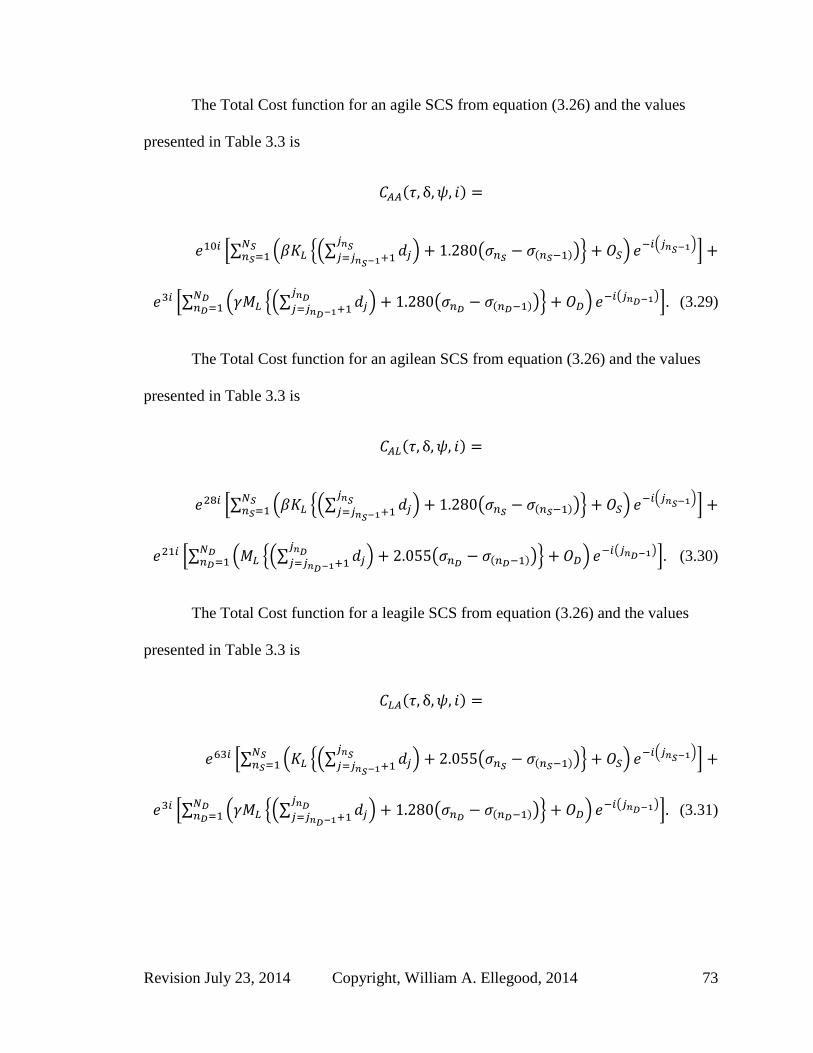
Revision July 23, 2014 Copyright, William A. Ellegood, 2014 73
The Total Cost function for an agile SCS from equation (3.26) and the values
presented in Table 3.3 is
( )
[∑ ( {(∑
) (
( ))} ) ( ) ]
[∑ ( {(∑
) (
( ))} ) ( )]. (3.29)
The Total Cost function for an agilean SCS from equation (3.26) and the values
presented in Table 3.3 is
( )
[∑ ( {(∑
) (
( ))} ) ( ) ]
[∑ ( {(∑
) (
( ))} ) ( )] (3.30)
The Total Cost function for a leagile SCS from equation (3.26) and the values
presented in Table 3.3 is
( )
[∑ ( {(∑
) (
( ))} ) ( ) ]
[∑ ( {(∑
) (
( ))} ) ( )] (3.31)

74 Copyright, William A. Ellegood, 2014 Revision July 23, 2014
The Total Cost function for a lean SCS from equation (3.26) and the values
presented in Table 3.3 is
( )
[∑ ( {(∑
) (
( ))} ) ( ) ]
[∑ ( {(∑
) (
( ))} ) ( )]. (3.32)
3.5 Model analysis framework
To evaluate the impact supply chain and product characteristics have on SCS
selection, this research identifies the SCS that results in lowest Total Cost while varying
four key characteristics. The four key characteristics are: ratio of manufacturing cost to
purchased material cost (RMP), demand forecast error, lean index and the cost of capital.
RMP is defined as the ratio of demand side manufacturing cost of the lean SCS to the
supply side purchased material cost of a lean SCS,
. (3.33)
RMP is similar to the value-added capacity characteristic considered by Li and
O’Brien (2001), where the value-added capacity for a product is determined by the ratio
of materials costs to finished product price. The RMP characteristic allows examination
of how the location of where costs are incurred in a supply chain impacts SCS selection.
When the lean index is small and RMP is less than 1, an agile SCS could result in a lower
total supply chain cost than a lean SCS, because of the cost advantage of a shorter supply
chain.

Revision July 23, 2014 Copyright, William A. Ellegood, 2014 75
The model in this research uses the measurement of demand forecast error to
define the level of demand uncertainty, as the value of demand forecast error increases as
the level of demand uncertainty increases. According to the Fisher Model when demand
uncertainty is high a product should be served with an agile SCS. The model in this
research should demonstrate that as the demand forecast error increases the Total Cost of
an agile SCS should decrease relative to a lean SCS.
The supply side lean index characteristic is the ratio of purchased material cost
for an agile SCS to a lean SCS, and the demand side lean index is the ratio of
manufacturing cost for an agile SCS to a lean SCS. The main advantage of a lean SCS is
the lower manufacturing and purchased material cost per unit; however, this advantage
comes with the higher financial cost associated from incurring costs earlier as the result
of the longer supply chain. If all parameters are equal, then with the longer supply chain
the Total Cost of a lean SCS would be greater than that of an agile SCS. An agilean SCS
and a leagile SCS would shorten the supply chain relative to a lean SCS, but both allow
the supply chain to still realize a portion of the lower total production cost advantage of a
lean SCS. For example, a supply chain may achieve a lower Total Cost relative to a lean
SCS by adopting an agilean SCS when the majority of the product’s costs are incurred
late in the supply chain (high RMP). In this case, the shorter agilean SCS relative to a
lean SCS would delay the point in time when supply side costs are incurred relative to a
lean SCS, while an agilean SCS would realize the lower demand side manufacturing
costs of the lean SCS, when all other terms are equal. For similar reasons, a leagile SCS
may result in a lower Total Cost than a lean SCS when RMP is low. The advantage of the
leagile SCS results from a shorter overall supply chain length than a lean SCS and delays

76 Copyright, William A. Ellegood, 2014 Revision July 23, 2014
the point in time when demand side and supply side costs are incurred relative to a lean
SCS, when all other terms are equal.
The cost of capital (CoC) as defined for this research is more than just the time
value of money, but also represents a measurement of the risk of holding inventory. The
risk of holding inventory increases when a product is subject to spoilage or the
probability of theft is high. This risk would also increase for those products in industries
where technology uncertainty is high, such as the computer or electronics industry.
Therefore, as the cost of capital increases, the cost advantage of the shorter agile SCS
should increase.
To simulate a variety of possible supply chain scenarios, the research considers a
low, medium, and high value for RMP, lean index, demand forecast error, and cost of
capital. The low RMP value describes a supply chain where 90% of the total unit costs
are in purchased material cost and 10% of the total unit costs are incurred at the
manufacturer. The medium RMP value reflects a supply chain where supplier and
manufacturer costs are equal. The high RMP value describes a supply chain where
purchased material costs are 10% of the total unit costs and 90% of the total unit costs are
incurred at the manufacturer. In practice, when a lean SCS provides a significant cost
advantage compared to the other supply chain strategies and a firm chooses a strategy
other than a lean SCS, then the firm’s primary supply chain objective is most likely not
total cost minimization. In those cases a model other than the one presented in this
research should be employed to assist the firm in selecting the correct SCS. For this
dissertation the model objective is cost minimization; therefore the lean index values
considered are relatively low. The three values for demand forecast error are derived
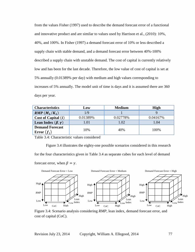
Revision July 23, 2014 Copyright, William A. Ellegood, 2014 77
from the values Fisher (1997) used to describe the demand forecast error of a functional
and innovative product and are similar to values used by Harrison et al., (2010): 10%,
40%, and 100%. In Fisher (1997) a demand forecast error of 10% or less described a
supply chain with stable demand, and a demand forecast error between 40%-100%
described a supply chain with unstable demand. The cost of capital is currently relatively
low and has been for the last decade. Therefore, the low value of cost of capital is set at
5% annually (0.01389% per day) with medium and high values corresponding to
increases of 5% annually. The model unit of time is days and it is assumed there are 360
days per year.
Characteristics Low Medium High
RMP ( ⁄ ) 1/9 1 9
Cost of Capital ( ) 0.01389% 0.02778% 0.04167%
Lean Index ( ) 1.01 1.02 1.04
Demand Forecast
Error ( ) 10% 40% 100%
Table 3.4: Characteristic values considered
Figure 3.4 illustrates the eighty-one possible scenarios considered in this research
for the four characteristics given in Table 3.4 as separate cubes for each level of demand
forecast error, when .
Figure 3.4: Scenario analysis considering RMP, lean index, demand forecast error, and
cost of capital (CoC).
High
CoC Low High Low
Lean
Index
RMP
Low
Demand Forecast Error = Low
CoC Low High Low
High
Lean
Index
RMP
Low
High
Demand Forecast Error = Medium
CoC Low High Low
High
Lean
Index
RMP
Low
High
Demand Forecast Error = High
High

78 Copyright, William A. Ellegood, 2014 Revision July 23, 2014
4. Examining the Fisher Model (lean and agile SCS only)
Question Q1 is addressed by this chapter: Under what circumstances does a
supply chain with a misaligned SCS and product type outperform a supply chain with an
aligned SCS and product type?
The primary purpose of this chapter is to identify the scenarios such that (i) the
Total Cost of an agile SCS is lower than that of a lean SCS for a product with functional
demand characteristics, and (ii) the Total Cost of a lean SCS is lower than that of an agile
SCS for a product with innovative demand characteristics. The secondary purpose of this
chapter is to examine the SCS, lean or agile, which a supply chain would move towards
in response to changes in demand, product cost, lead time, and service level.
4.1 Problem description
This chapter considers the special case where expected demand and expected
demand forecast error are constant for the forecast period [ ] and actual demand is
normally distributed about expected demand, , during the forecast period: [ ].
The expected demand rate for the forecast period [ ] is
∫ ( )
. (4.1)
With time measured in days, is daily expected demand and
. (4.2)
With expected demand forecast error constant for the forecast period,
. (4.3)

Revision July 23, 2014 Copyright, William A. Ellegood, 2014 79
The standard deviation of actual daily demand about expected demand when both
expected demand and demand forecast error are constant for the forecast period is
defined by substituting equations (4.1) and (4.2) into equation (3.14),
. (4.4)
The standard deviation of daily demand is constant for the forecast period and the
daily expected demands are assumed mutually independent. Therefore, the standard
deviation of demand over the order period for each side of the supply chain is the product
of and the square root of the length of each order period. From equation (3.16), the
standard deviation of demand for every demand side order period is
√∑
√
. (4.5)
From equation (3.16), the standard deviation of demand for every supply side order
period is
√∑
√
. (4.6)
When expected demand and demand forecast error are constant for the forecast
period, the change in safety stock inventory level from period to period, given by
equations (3.20) and (3.21), is zero for both inventory locations (manufacturer and
customer) and only the safety stock level for the first order period needs to be
determined.

80 Copyright, William A. Ellegood, 2014 Revision July 23, 2014
The Total Cost function when expected demand and demand forecast error are
constant, ( ), is determined by substituting equations (4.2), (4.3), (4.5), and
(4.6) into equation (3.26),
( ) ( ) [∑ ( {(∑
) }
) ( )] ( ) [∑ ( {(∑
) } )
( )].
(4.7)
The summations ∑
∑
( ) in equation (4.7), are the total
expected demand during a demand side and supply side order period, respectively. The
total expected demand for every demand side order period is the product of the length of
the demand side order period, equation (3.2), and expected daily demand ,
∑
. (4.8)
The total expected demand for every supply side order period is the product of the
length of the order period, equation (3.4), and expected daily demand ,
∑
. (4.9)

Revision July 23, 2014 Copyright, William A. Ellegood, 2014 81
The Total Cost function ( ) can be simplified further by substituting
equations (3.1), (3.3), (4.8) and (4.9) into equation (4.7),
( )
( ) ( [∑
( )
] ∑
( )
)
( ) ( [∑
( )
] ∑
( )
). (4.10)
Each summation in equation (4.7) is a partial sum of a geometric series with the
general form
where . (4.11)
Riddle (1979) described the partial sum ( ) for the first m terms of a geometric series
where as
( )
( ). (4.12)
The value of for the series ∑
( )
are
,
, and
and the partial sum of the geometric series is
∑
( )
( )
( )
( (
)
)
(
)
( )
(
)
. (4.13)
Using the same technique to transform the remaining three summations in
equation (4.7) and factoring out common terms results in the following Total Cost

82 Copyright, William A. Ellegood, 2014 Revision July 23, 2014
function when expected demand and forecast error are constant for the forecast period
[ ],
( ) ( ) [ ( ( )
(
)
√
)
( )
(
)
]
( ) [ ( ( )
(
)
√
)
( )
(
)
]. (4.14)
Let ( )
(
)
and ( )
(
)
, therefore
( )
( ) [ (
√
) ]
( ) [ (
√
) ]. (4.15)
In the simplest terms, ( ) is the sum of the total NPV supply chain
production cost, ( ), and the total NPV supply chain order processing
cost, ( ). The total NPV supply chain production cost is
( ) ( ) [ ( ) (
√
) (
√
)] (4.16)
where the first term is the total NPV supply side production cost
( ) (
√
) (4.17)

Revision July 23, 2014 Copyright, William A. Ellegood, 2014 83
and the second term is the total NPV demand side production cost
( ) (
√
). (4.18)
The total NPV supply chain order processing cost is
( ) ( )[ ( ) ], (4.19)
where the first term is the total NPV supply side order processing cost
( ) (4.20)
and the second term is total NPV demand side order processing cost
( ). (4.21)
( ) and ( ) are supply chain cost components dependent upon the
number of order periods, and ; as and increases, with all other terms held
constant, ( ) decreases and ( ) increases. If ( ) is a convex
function, then there are values for and that minimize ( ); and
respectively. The values for and
are positive integers [ ].
H1: When demand is constant there are values for the number of ordering periods,
and , which minimize ( ) for the forecast period [ ].
Proof: ( ) is a convex function if ( ) decreases at a decreasing rate and
( ) increases at an increasing rate as the value for and
increases.
Step 1: ( ) decreases at a decreasing rate as or increases for
.

84 Copyright, William A. Ellegood, 2014 Revision July 23, 2014
The function ( ) is such that if decreases at a decreasing rate with respect to
, then must decrease at a decreasing rate with respect to . Therefore, the
following proof only examines .
decreases at a decreasing rate with respect to
for all values of when
and
.
( ) (
( )
(
)
√
)
( ) ( )(
(
)
) ( ) √
(
√
)
[ ( ) ( )]
[
(
)
(
)
]
[ ( ) √
] [
√ ]
The value of
is the sum of two terms that are each the product of a positive term and
a negative term; hence, the sum of two negative terms must always be less than zero, for
,
[ ][ ] [ ][ ] .

Revision July 23, 2014 Copyright, William A. Ellegood, 2014 85
( ) ( )
(
(
)
(
)
(
)
)
( ) √
(
√ )
( ) ( )
(
( (
) (
) )
(
)
( (
)
(
) )
(
)
)
( ) √ (
√
)
[ ( ) ( )] [
(
)
(
)
(
)
(
)
]
[ ( ) √ ] [
√
]
The value of
is the sum of two terms that are each the product of a two positive
terms; hence, the sum of two positive terms must always be greater than zero, subject to
,
[ ][ ] [ ][ ] .
From Step 1,
and
for all values of ; therefore,
decreases at a decreasing rate for all values of . From similar
reasoning, for all values of must also decrease at a decreasing rate.

86 Copyright, William A. Ellegood, 2014 Revision July 23, 2014
Therefore, Step 1 is accepted: ( ) decreases at a decreasing rate as or
increases for . The limit of ( ) as
establishes the lower bound for the total NPV supply chain production
cost as
( ) ( ) [ ( ) (( )
( )
)
(( )
( )
)]. (4.22)
The upper bound for the total NPV supply chain production cost is when both
equal one and is
( ) ( ) [ ( ) (
√ ) (
√ )]. (4.23)
Step 2: ( ) increases as an increasing rate as or increases for
.
The function ( ) is such that if increases at an increasing rate with
respect to , then must increase at an increasing rate with respect to Therefore,
the following proof only examines .
increases at an increasing rate with respect to
for all values of when
and
.
( ) ( )
(
)
( )( )(
(
)
)

Revision July 23, 2014 Copyright, William A. Ellegood, 2014 87
[ ( )( )]
[
(
)
]
The value of
is the product of a two positive terms; therefore, it must always be
greater than zero, for ,
[ ][ ] .
( )( )
(
(
)
)
[ ( )( )]
[
(
)
(
)
(
)
]
The value of
is the product of a two positive terms; therefore, it must always be
greater than zero, for ,
[ ][ ] .
From Step 2,
and
for all values of ; therefore,
increases at an increasing rate for all values of . From similar
reasoning, for all values of must also increase at an increasing rate.
Therefore, Step 2 is accepted: ( ) increases at an increasing rate as or
increases for . The limit of ( ) as
defines the upper bound of the total NPV supply chain order processing cost as

88 Copyright, William A. Ellegood, 2014 Revision July 23, 2014
( ) ( )( )
( )(
( ) ). (4.24)
The lower bound for the total NPV supply chain order processing cost is when
both equal one and is
( ) ( )( ( ) ). (4.25)
Step 1 and Step 2 together provide the Proof: ( ) is a convex function
with ( ) decreasing at a decreasing rate and ( ) increasing at an
increasing rate as the value for and
increases; therefore, H1 is accepted.
The first derivative of ( ) with respect to is
( )
(4.26)
The result of equation (4.26) set equal to zero and simplified is
√
(
)
( )
. (4.27)
A closed form solution for the optimal number of order periods, , cannot be
determined in general from equation (4.27); therefore, for the analysis in Chapters 4-6,
the optimal values of
to minimize the Total Cost are found by complete
enumeration of all possible values (where
and
are integers).

Revision July 23, 2014 Copyright, William A. Ellegood, 2014 89
4.2 Scenario analysis
Consider a baseline supply chain setting where the forecast period is 180 days,
the lean SCS total production cost, , to deliver a single product to the customer is
$100, the average demand is 275 units per day (approximately 100,000 units per year),
demand forecast error during the forecast period is constant, the ordering cost
are both $200, and the lean index for the supply side and demand side are
equal, . The values for supply side and demand side lead times and service levels
for each SCS are taken from Table 3.3. Using this as a baseline supply chain setting, the
Total Cost function for an agile SCS is
( ) [ (
√ ) ] [ (
) (
√ ) ]. (4.28)
The Total Cost function for a lean SCS is
( ) [ (
√ ) ] [ (
) (
√ ) ]. (4.29)
and
for each of the scenarios presented in Figure 3.4 are found by the
complete enumeration of equations (4.28) and (4.29) for each SCS. The Total Cost of
each SCS are compared ( ( )(
) ( )(
))
and the SCS with the lowest Total Cost is shown in Figure 4.1 for each of the scenarios
described in Figure 3.4. (LL denotes a lean SCS with a lean strategy employed on both

90 Copyright, William A. Ellegood, 2014 Revision July 23, 2014
the demand and supply side of the supply chain and AA denotes an agile SCS with an
agile strategy adopted on both the demand and supply side of the supply chain.)
Demand Forecast Error
Low
Medium
High
Cost of Capital Cost of Capital Cost of Capital
Low Med. High Low Med. High Low Med. High
Lean
High RMP
High LL LL LL
LL LL LL
LL LL LL
Med. LL LL LL
LL LL LL
LL LL LL
Low LL LL LL
LL LL LL
LL LL LL
Med. RMP
High LL LL LL
LL LL LL
LL LL LL Index Med. LL LL AA
LL LL AA
LL AA AA
Low LL LL AA
LL AA AA
LL AA AA
Low RMP
High LL LL AA
LL AA AA
AA AA AA
Med. LL AA AA
AA AA AA
AA AA AA
Low AA AA AA AA AA AA AA AA AA
Figure 4.1: SCS with the lowest Total Cost (Lean and Agile only)
Some general managerial insights can be learned from the examination of Figure
4.1 concerning the SCS that results in the lowest Total Cost, with respect to demand
forecast error, cost of capital, lean index and RMP. With all other terms held constant, as
demand forecast error decreases from high to low, the SCS that results in the lowest Total
Cost may move from an agile SCS to a lean SCS. Figure 4.1 shows support for the Fisher
Model when the objective is cost minimization, for supply chains where the lean index is
not at a high level, that an agile SCS is the preferred SCS for products with high demand
forecast error and a lean SCS is the preferred SCS for products with low demand forecast
error.
Agile SCS
(AA)
Lean SCS
(LL)
Revision July 23, 2014 Copyright, William A. Ellegood, 2014 91
As the cost of capital decreases, the SCS that results in the lowest Total Cost may
move from an agile SCS to a lean SCS. In addition, for those supply chains where a large
percentage of the production costs are incurred at the supplier (low RMP), an agile SCS is
more likely to result in a lower Total Cost than a lean SCS. However, when a large
percentage of the production costs are located closer to the customer (high RMP), a lean
SCS is more likely to result in a lower Total Cost. Lastly, as the ratio of production cost
for an agile SCS to a lean SCS increases, a lean SCS is more likely to result in a lower
Total Cost than an agile SCS.
One of the key product characteristics Fisher (1997) used to distinguish a product
as functional or innovative was demand forecast error, where the demand forecast error
was less than 10% for a functional product and 40% or more for an innovative product.
As discussed earlier, not all products are easily classified as functional or innovative.
This leads to the question of when does an agile SCS result in a lower Total Cost than a
lean SCS for a product with functional demand characteristics? From the discussion of
Figure 4.1, as demand forecast error decreases from high to low, and without
consideration of the other characteristics, the SCS which results in the lowest Total Cost
may move from an agile SCS to a lean SCS. However, when considering the other three
characteristics examined in this research (lean index, RMP, and cost of capital) in
addition to a low level of demand forecast error, we find that a lean SCS does not always
result in a lower Total Cost than an agile SCS (8 of 27 scenarios).

92 Copyright, William A. Ellegood, 2014 Revision July 23, 2014
4.2.1 Low demand forecast error
H2: The Total Cost of an agile SCS can be less than that of a lean SCS when demand
forecast error is low, and an agile SCS becomes more attractive as RMP decreases, lean
index decreases, and cost of capital increases.
From Figure 4.1, for a supply chain with low RMP, low lean index, and high cost
of capital, an agile SCS does result in a lower Total Cost than a lean SCS when the
demand forecast error is low, like that associated with a functional product. To examine
H2 further, consider the scenario with low RMP, low lean index, high cost of capital, and
low demand forecast error. Figure 4.2 presents the relative Total Cost difference of an
agile SCS compared to a lean SCS when one of these four characteristics is varied and
the other three characteristics are held constant. The relative Total Cost percent
difference, , of an agile SCS to a lean SCS is
( )(
) ( )(
)
( )(
) . (4.30)
Therefore, when is less than zero an agile SCS results in a lower Total Cost than a
lean SCS, and when is greater than zero a lean SCS results in a lower Total Cost
than an agile SCS. The horizontal axis of the upper left graph in Figure 4.2 indicates the
relative manufacturing cost, defined as the percentage of manufacturing costs to total
production costs for a lean SCS (note:
),
. (4.31)

Revision July 23, 2014 Copyright, William A. Ellegood, 2014 93
When the value of is 10%, RMP is at a low level (0.111); when the value of is
50%, RMP is at a medium level (1.0); and when the value of is 90%, RMP is at a
high level (9.0).
Figure 4.2: Value of when one characteristic is varied and the other three are fixed
with low RMP, low lean index, high cost of capital, and low demand forecast error.
Setting equations (4.28) and (4.29) equal to each other and with three of the four
characteristics held constant, we can determine the value of the fourth characteristic such
that the Total Cost of an agile SCS and a lean SCS are equal. The values for and
for each of the supply chain strategies when equals zero are determined by
complete enumeration. Consider the upper left graph in Figure 4.2, with low demand
forecast error, low lean index, and high cost of capital. In this case, for the RMP value of
approximately 17.03 ( ), the Total Cost of an agile SCS and a lean SCS
-2.5%
-2.0%
-1.5%
-1.0%
-0.5%
0.0%
0.5%
1.0%
1.5%
2.0%
2.5%
10% 30% 50% 70% 90%
ΦLL
,1
RMC
Agile
-2.5%
-2.0%
-1.5%
-1.0%
-0.5%
0.0%
0.5%
1.0%
1.5%
2.0%
2.5%
0% 20% 40% 60% 80% 100%
ΦLL
,1
Demand Forecast Error
Agile
-2.5%
-2.0%
-1.5%
-1.0%
-0.5%
0.0%
0.5%
1.0%
1.5%
2.0%
2.5%
1.01 1.02 1.03 1.04 1.05
ΦLL
,1
Lean Index
Agile
-2.5%
-2.0%
-1.5%
-1.0%
-0.5%
0.0%
0.5%
1.0%
1.5%
2.0%
2.5%
4% 6% 8% 10% 12% 14%
ΦLL
,1
Cost of Capital
Agile

94 Copyright, William A. Ellegood, 2014 Revision July 23, 2014
are equal. A RMP value of 17.03 is much larger than the RMP value identified as high in
Table 3.4, where the high RMP =9. Therefore, for a supply chain with low demand
forecast error, low lean index, high cost of capital, and the remaining supply chain
parameters are those described in Table 3.3, the RMP characteristics of the supply chain
needs to be very high (almost 95% of production costs at the manufacturer) before a lean
SCS results in a lower Total Cost than an agile SCS.
The demand forecast error value in Figure 4.2 where equals zero (upper
right graph) is -28.07%. As defined, the expected demand forecast error cannot be less
than zero; therefore, with low RMP, low lean index, high cost of capital, and the
remaining supply chain parameters described in Table 3.3, an agile SCS always results in
a lower Total Cost than a lean SCS.
When the lean index value in Figure 4.2 is 1.029 (lower left graph), a value
between the medium and high levels as described in Table 3.4, the Total Cost of an agile
SCS is equal to that of a lean SCS. The cost of capital value in Figure 4.2 (lower right
graph) where equals zero is 4.62% annually, which is less than the cost of capital
value defined as a low level in Figure 3.4, with low RMP, low demand forecast error, low
lean index and the remaining supply chain parameters described in Table 3.3.

Revision July 23, 2014 Copyright, William A. Ellegood, 2014 95
Figure 4.3: Cost of capital that makes as a function of the value of
( ) and the lean index value when demand forecast error is low as described in
Table 3.4.
Figure 4.3 shows the annual percent cost of capital where the Total Cost of an
agile SCS equals a lean SCS with respect to the and the lean index value for a
supply chain when the demand forecast error is low (10%). To interpret this surface
graph, for a point above the surface an agile SCS will result in a lower Total Cost, and for
a point below the surface a lean SCS results in a lower Total Cost (with low demand
forecast error). Figure 4.3 demonstrates that the choice between an agile SCS and a lean
SCS is more sensitive to (and RMP) as the lean index increases and less sensitive to
as the cost of capital increases.
4.2.2 High demand forecast error
The previous section examined the situations where an agile SCS results in a
lower Total Cost compared to a lean SCS for a product with functional demand
1.01
1.02
1.03
1.04
0
10
20
30
40
50
60
10% 20% 30% 40% 50% 60% 70%80%
90%
Lean Index
Co
st o
f C
apit
al (
pct
. pe
r ye
ar)
𝑅𝑀𝐶
Total Cost of Agile SCS = Lean SCS when Demand Forecast Error is Low
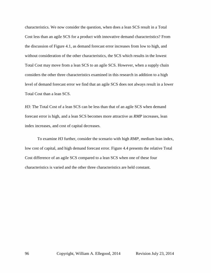
96 Copyright, William A. Ellegood, 2014 Revision July 23, 2014
characteristics. We now consider the question, when does a lean SCS result in a Total
Cost less than an agile SCS for a product with innovative demand characteristics? From
the discussion of Figure 4.1, as demand forecast error increases from low to high, and
without consideration of the other characteristics, the SCS which results in the lowest
Total Cost may move from a lean SCS to an agile SCS. However, when a supply chain
considers the other three characteristics examined in this research in addition to a high
level of demand forecast error we find that an agile SCS does not always result in a lower
Total Cost than a lean SCS.
H3: The Total Cost of a lean SCS can be less than that of an agile SCS when demand
forecast error is high, and a lean SCS becomes more attractive as RMP increases, lean
index increases, and cost of capital decreases.
To examine H3 further, consider the scenario with high RMP, medium lean index,
low cost of capital, and high demand forecast error. Figure 4.4 presents the relative Total
Cost difference of an agile SCS compared to a lean SCS when one of these four
characteristics is varied and the other three characteristics are held constant.

Revision July 23, 2014 Copyright, William A. Ellegood, 2014 97
Figure 4.4: Value of when one characteristic is varied and the other three are fixed
with RMP high, lean index medium, cost of capital low, and demand forecast error high.
As with H2, the value of a characteristic where equals zero is determined by
setting equations (4.28) and (4.29) equal to each other, with three of the four
characteristics held constant, and solving for the fourth characteristic. The values for
and for each of the supply chain strategies are determined by complete enumeration.
The RMP value where equals zero in Figure 4.4 (upper left graph) is -0.0015. The
value of RMP is bounded on the lower end at zero (when zero production costs are
incurred at the manufacturer and 100% of the production costs are at the supplier):
therefore, with high demand forecast error, low cost of capital, and medium lean index, a
lean SCS results in a lower Total Cost than an agile SCS independent of the RMP value.
The demand forecast error value where equals zero in Figure 4.4 (upper
right graph) is 249%, a level of demand forecast error far greater than the high level of
-0.5%
0.0%
0.5%
1.0%
1.5%
2.0%
2.5%
3.0%
10% 30% 50% 70% 90%
ΦLL
,1
RMC
-0.5%
0.0%
0.5%
1.0%
1.5%
2.0%
2.5%
3.0%
10% 30% 50% 70% 90%
ΦLL
,1
Demand Forecast Error
-0.5%
0.0%
0.5%
1.0%
1.5%
2.0%
2.5%
3.0%
1.01 1.02 1.03 1.04
ΦLL
,1
Lean Index
-0.5%
0.0%
0.5%
1.0%
1.5%
2.0%
2.5%
3.0%
5% 10% 15% 20%Φ
LL,1
Cost of Capital
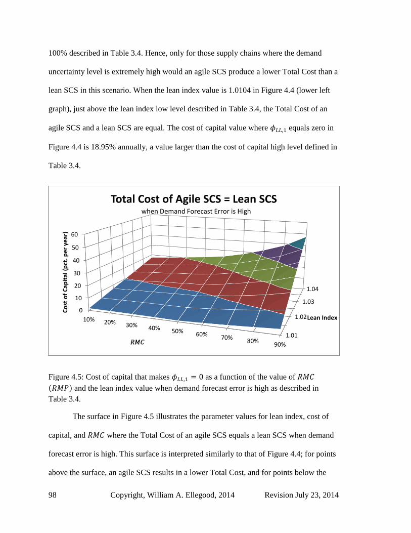
98 Copyright, William A. Ellegood, 2014 Revision July 23, 2014
100% described in Table 3.4. Hence, only for those supply chains where the demand
uncertainty level is extremely high would an agile SCS produce a lower Total Cost than a
lean SCS in this scenario. When the lean index value is 1.0104 in Figure 4.4 (lower left
graph), just above the lean index low level described in Table 3.4, the Total Cost of an
agile SCS and a lean SCS are equal. The cost of capital value where equals zero in
Figure 4.4 is 18.95% annually, a value larger than the cost of capital high level defined in
Table 3.4.
Figure 4.5: Cost of capital that makes as a function of the value of
( ) and the lean index value when demand forecast error is high as described in
Table 3.4.
The surface in Figure 4.5 illustrates the parameter values for lean index, cost of
capital, and where the Total Cost of an agile SCS equals a lean SCS when demand
forecast error is high. This surface is interpreted similarly to that of Figure 4.4; for points
above the surface, an agile SCS results in a lower Total Cost, and for points below the
1.01
1.02
1.03
1.04
0
10
20
30
40
50
60
10% 20% 30% 40% 50% 60% 70%80%
90%
Lean Index
Co
st o
f C
apit
al (
pct
. pe
r ye
ar)
𝑅𝑀𝐶
Total Cost of Agile SCS = Lean SCS when Demand Forecast Error is High

Revision July 23, 2014 Copyright, William A. Ellegood, 2014 99
surface a lean SCS results in a lower Total Cost. Figure 4.4 illustrates that the choice
between an agile SCS and a lean SCS is more sensitive to lean index as increases
and is less sensitive to lean index as the cost of capital increases.
4.3 Sensitivity analysis
This section provides a sensitivity analysis of the baseline supply chain setting
from section 4.2 to examine the impact of total production cost relative to ordering cost,
expected demand, lead time, and service level on the relative cost difference between a
lean SCS and an agile SCS. The purpose of the sensitivity analysis is to provide insight
into how a change in the value of a single aspect of the supply chain (demand, product
cost, or supply chain aspect) impacts the supply chain’s propensity towards either a lean
or an agile SCS, when only one of the four characteristics is varied (RMP, lean index,
cost of capital, and demand forecast error) and the other three characteristics are held
constant at their medium level, as defined in Table 3.4.
The multiple lines in each of Figures 4.6-4.21 illustrate the value of as one
aspect of the supply chain is varied for several different levels of one characteristic, with
the other three characteristics held at their medium level and other parameters at the
baseline supply chain setting as presented in section 4.2. When is greater than zero
a lean SCS results in a lower Total Cost and when is less than zero an agile SCS
should be employed to minimize Total Cost.
4.3.1 Total production cost to total order processing cost
The Total Cost function considers two major categories of costs: (i) production
costs for supply side purchasing and demand side manufacturing, where the values of

100 Copyright, William A. Ellegood, 2014 Revision July 23, 2014
these costs are dependent upon the SCS, and (ii) total order processing cost for the
demand side and supply side, which are assumed to be independent of the SCS.
Therefore, as the ratio of total production cost to total order processing cost increases for
a supply chain, the likelihood increases that a lean SCS will result in a lower Total Cost
than an agile SCS.
H4: As the ratio of total production cost to total order processing cost increases, the
supply chain’s propensity towards a lean SCS increases.
In the baseline supply chain setting presented in section 4.2, the total production
cost per unit is and the total order processing cost per order is
. Therefore, the baseline ratio of total production cost to total order processing
cost is 0.25. The values for total production cost and total order processing cost that
define the x-axis of Figures 4.6-4.9 are given in Table 4.1.
Ratio of total production
cost to total order
processing cost
0.0025 0.0125 0.0250 0.1250 0.2500
Total Production Cost $1 $5 $10 $50 $100
Total order processing
cost
$400 $400 $400 $400 $400
Table 4.1: Legend for the x-axis of Figures 4.6-4.9; showing the ratio of total production
cost to total order processing cost.

Revision July 23, 2014 Copyright, William A. Ellegood, 2014 101
Figure 4.6: Value of with respect to the ratio of total production cost to total order
processing cost for different RMP levels.
From Figure 4.6, when the supply chain structure is such that when the majority
of the total production costs are incurred at the manufacturer (i.e. RMP is large), the total
order processing cost must be much larger than the total production cost for an agile SCS
to result in a lower Total Cost than a lean SCS. In turn, when the vast majority (90%+) of
the total production costs of a product are incurred at the supplier (i.e. ⁄ )
and the lean index, cost of capital and the demand forecast error at a medium level per
Table 3.4, an agile SCS results in a lower Total Cost than a lean SCS and this is
independent of the value of the ratio of total production cost to total order processing
cost. However, for all other supply chain strategies a significant change in supply chain
structure or in the ratio of total production cost to total order processing cost can impact
the SCS that results in the lowest Total Cost .
-3.0%
-2.0%
-1.0%
0.0%
1.0%
2.0%
0 0.05 0.1 0.15 0.2 0.25
𝜙LL
,1
Total production cost / Total order processing cost
90/10
70/30
50/50
30/70
10/90
RMP

102 Copyright, William A. Ellegood, 2014 Revision July 23, 2014
Figure 4.7: Value of with respect to the ratio of total production cost to total order
processing cost for different demand forecast error levels.
Figure 4.7 illustrates the impact to when the ratio of total production cost to
total order processing cost and demand forecast error vary with all other terms held
constant. When the demand forecast error is stable, the SCS that results in the lowest
Total Cost is relatively insensitive to the ratio of total production cost to total order
processing cost when the ratio is greater than 0.025 or the total order processing cost is
not more than 40 times the total production cost. When the demand forecast error is
unstable, the SCS is relatively insensitive to the ratio of production cost to order
processing cost, when the ratio is greater than 0.10 or the total order processing cost is
not more than 10 times the total production cost. Also, when the ratio of total production
cost to total order processing cost is greater than approximately 2.0 (not shown in Figure
4.7) a lean SCS results in a lower Total Cost than an agile SCS independent of the level
of demand forecast error, with all other terms constant.
-3.0%
-2.0%
-1.0%
0.0%
1.0%
2.0%
0.00 0.05 0.10 0.15 0.20 0.25
𝜙LL
,1
Total production cost / Total order processing cost
0%
20%
40%
60%
80%
100%
Demand Forecast
Error

Revision July 23, 2014 Copyright, William A. Ellegood, 2014 103
Figure 4.8: Value of with respect to the ratio of total production cost to total order
processing cost for different lean index levels.
Figure 4.8 shows that when the lean index is high a lean SCS results in the lower
Total Cost, and when the lean index is low an agile SCS results in the lower Total Cost,
independent of the values considered for the ratio of total production cost to total order
processing cost, when all other parameters are constant.
-3%
-2%
-1%
0%
1%
2%
3%
0.00 0.05 0.10 0.15 0.20 0.25
𝜙LL
,1
Total production cost / Total order processing cost
1.04%
1.03%
1.02%
1.01%
1.00%
Lean Index
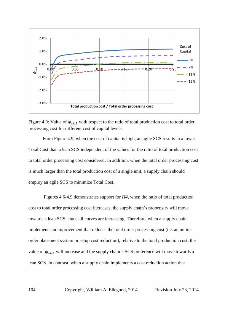
104 Copyright, William A. Ellegood, 2014 Revision July 23, 2014
Figure 4.9: Value of with respect to the ratio of total production cost to total order
processing cost for different cost of capital levels.
From Figure 4.9, when the cost of capital is high, an agile SCS results in a lower
Total Cost than a lean SCS independent of the values for the ratio of total production cost
to total order processing cost considered. In addition, when the total order processing cost
is much larger than the total production cost of a single unit, a supply chain should
employ an agile SCS to minimize Total Cost.
Figures 4.6-4.9 demonstrates support for H4, when the ratio of total production
cost to total order processing cost increases, the supply chain’s propensity will move
towards a lean SCS, since all curves are increasing. Therefore, when a supply chain
implements an improvement that reduces the total order processing cost (i.e. an online
order placement system or setup cost reduction), relative to the total production cost, the
value of will increase and the supply chain’s SCS preference will move towards a
lean SCS. In contrast, when a supply chain implements a cost reduction action that
-3.0%
-2.0%
-1.0%
0.0%
1.0%
2.0%
0.00 0.05 0.10 0.15 0.20 0.25
𝜙LL
,1
Total production cost / Total order processing cost
3%
7%
11%
15%
Cost of Capital

Revision July 23, 2014 Copyright, William A. Ellegood, 2014 105
reduces the total production cost relative to the total order processing cost of a product
the supply chain’s propensity will move towards an agile SCS.
4.3.2 Average daily demand
The second aspect of the supply chain to be examined in the sensitivity analysis is
the impact of the value of expected demand on the relative cost difference between the
Total Cost of an agile SCS and a lean SCS. When all other parameters are constant, an
increase in expected daily demand will increase the total production cost side of the
model without impacting the total order processing cost, because total order processing
cost is modeled independent of expected demand. To offset this rise in the total
production cost a supply chain could increase the number of orders placed during the
forecast period, thereby delaying when some of the production costs are incurred.
However, the model in this dissertation does not allow a supply chain to place more than
one order per day. Once the expected demand value reaches a level where orders are
placed daily, any additional increase in expected demand has little to no impact on the
relative cost difference between an agile SCS and a lean SCS.
H5: As the expected daily demand rate increases, the supply chain’s propensity towards a
lean SCS increases.
The expected daily demand rate in the baseline supply chain setting presented in
this dissertation is 275 units or 99,000 units annually. The values of expected daily
demand rate and annual demands for 360 days per year considered in Figures 4.10-4.13
are given in Table 4.2.

106 Copyright, William A. Ellegood, 2014 Revision July 23, 2014
Expected daily
demand rate 10 50 100 500 1,000
Expected annual
demand 3,600 18,000 36,000 180,000 360,000
Table 4.2: Legend for the x-axis of Figures 4.10-4.14 with expected daily demand and
annual demand.
Figure 4.10: Value of with respect to the expected daily demand rate for different
RMP levels.
From Figure 4.10, for a given value of RMP when the expected daily demand rate
is changed significantly there was only a small impact to the value of , except for
small expected daily demand rates (<50). For supply chain structures where the vast
majority (≥90%) of total production costs are incurred at the supplier, an agile SCS
results in a slightly lower Total Cost than a lean SCS for all the values of expected daily
demand rate considered in this analysis. In addition, for supply chain structures where the
vast majority (≥90%) of total production costs are incurred at the manufacturer, a lean
SCS results in a slightly lower Total Cost (at worst about 1%) than an agile SCS for all
the values of expected daily demand rate considered in this analysis.
-2.0%
-1.5%
-1.0%
-0.5%
0.0%
0.5%
1.0%
1.5%
2.0%
0 100 200 300 400 500 600 700 800 900 1000
𝜙LL
,1
Expected daily demand
90/10
70/30
50/50
30/70
10/90
RMP

Revision July 23, 2014 Copyright, William A. Ellegood, 2014 107
Figure 4.11: Value of with respect to the expected daily demand rate for different
demand forecast error levels.
Figure 4.11 shows that the sensitivity of relative Total Cost to a change in the
expected daily demand rate is greatest, although small, when demand forecast error is
greater than 20% and expected daily demand is less than 400 units. For expected daily
demand rates greater than 400 units a lean SCS results in a slightly lower Total Cost than
an agile SCS (<1%) and the relative Total Cost difference is not sensitive to an increase
in the expected daily demand rate. When the demand forecast error is less than 20% a
lean SCS results in a slightly lower Total Cost than an agile SCS independent of the
expected daily demand rate, when all others terms are constant.
-2.0%
-1.5%
-1.0%
-0.5%
0.0%
0.5%
1.0%
1.5%
2.0%
0 100 200 300 400 500 600 700 800 900 1000
𝜙LL
,1
Expected daily demand
0%
20%
40%
60%
80%
100%
Demand Forecast
Error

108 Copyright, William A. Ellegood, 2014 Revision July 23, 2014
Figure 4.12: Value of with respect to the expected daily demand rate for different
lean index levels.
Similar to Figure 4.8, in Figure 4.12 a small change in the lean index results in a
relatively large change in the value of . For values of expected daily demand rates
greater than 100 units, an increase in expected daily demand rate has a very small impact
on the relative Total Cost percent difference, for a given lean index value.
-3%
-2%
-1%
0%
1%
2%
3%
0 100 200 300 400 500 600 700 800 900 1000
𝜙LL
,1
Expected daily demand
1.04%
1.03%
1.02%
1.01%
1.00%
Lean Index
Revision July 23, 2014 Copyright, William A. Ellegood, 2014 109
Figure 4.13: Value of with respect to the expected demand rate for different cost of
capital levels.
Figure 4.13 shows that for expected daily demand rate values greater than 100 and
when the cost of capital is less than 11%, a lean SCS results in the lowest Total Cost
when compared to an agile SCS. When the cost of capital is high an agile SCS results in a
slightly lower Total Cost than a lean SCS independent of the expected daily demand rates
considered here.
Figure 4.10-4.13 demonstrates support for H5 when expected daily demand rate
increases the supply chain’s propensity moves towards a lean SCS, since all curves are
increasing. Therefore, as the value of expected daily demand rate increases the likelihood
that a lean SCS will minimize Total Cost relative to an agile SCS increases. However, the
relative Total Cost difference between the supply chain strategies is constrained by the
frequency at which orders could be placed (at most once per day).
-2.0%
-1.5%
-1.0%
-0.5%
0.0%
0.5%
1.0%
1.5%
2.0%
0 100 200 300 400 500 600 700 800 900 1000
𝜙LL
,1
Expected daily demand
3%
7%
11%
15%
Cost of Capital

110 Copyright, William A. Ellegood, 2014 Revision July 23, 2014
4.3.3 Supply side lead time
The next aspect of the supply chain examined in this section is the ratio of supply
side lead times between the supply chain strategies. The baseline supply chain setting
models the lean SCS with a long supply side lead time, days, such as for an
off-shore supplier. The agile SCS assumes a shorter supply side lead time, days,
such as for a domestic supplier. Obviously firms employing a lean SCS are not only
located off-shore (with long lead times); but might be located domestically with a shorter
lead time or in a location where the lead time is longer than that considered in the
baseline supply chain setting. Supply chain responsiveness is the primary objective of an
agile SCS and a secondary objective of a lean SCS. Longer lead times increase the
inventory costs of a supply chain and increase the risk associated with obsolescence and
spoilage. An increase in the ratio
indicates the supply side lead time of the lean SCS
lengthens relative to the supply side lead time of the agile SCS, resulting in an increase in
the inventory costs of the lean SCS relative to the agile SCS. Therefore, lengthening the
lean SCS supply chain relative to the supply chain length of the agile SCS will result in a
decrease in the relative Total Cost percent difference between the supply chain strategies.
H6: When the ratio
increases, the supply chain’s propensity towards an agile SCS
increases.
For the baseline supply chain setting the supply lead time ratio (for a lean SCS to
an agile SCS) is 60/7 = 8.57. The values for the lean SCS supply side lead time and the
agile SCS supply side lead times used to develop the x-axis values for
in Figures
4.14-4.17, are given in Table 4.3.

Revision July 23, 2014 Copyright, William A. Ellegood, 2014 111
⁄ 1 2 4 8 12 16
7 14 28 56 84 112
7 7 7 7 7 7
Table 4.3: Legend for the x-axis of Figure 23-26, ratio of the lean SCS supply side lead
time to the agile supply side lead time.
Figure 4.14: Value of with respect to the ratio
for different RMP levels.
From Figure 4.14, when the supply chain structure is such that the majority of the
total production costs are incurred at the manufacturer (high RMP), the value of is
insensitive to changes in the supply side lead time ratio and a lean SCS results in a
slightly lower Total Cost than an agile SCS for the supply side lead time ratios
considered. As the supply chain structure moves from a RMP value of 90/10 to 10/90, the
sensitivity of to the supply side lead time ratio increases. When the lean SCS supply
side lead time equals the agile SCS supply side lead time, the value of is about 1%
for all values of RMP considered. However, Figure 4.14 supports hypothesis H6 that as
the ratio of the supply side lead time for a lean SCS to that of an agile SCS increases the
propensity of a supply chain is to move towards an agile SCS.
-2%
-1%
0%
1%
2%
1 4 7 10 13 16
𝜙LL
,1
LL,S / LA,S
90/10
70/30
50/50
30/70
10/90
RMP

112 Copyright, William A. Ellegood, 2014 Revision July 23, 2014
Figure 4.15: Value of with respect to the ratio
for different demand forecast
error levels.
Figure 4.15 indicates even when the demand forecast error is 0%, the value of
decreases as the supply side lead time ratio increases. Therefore, an agile SCS
results in a lower Total Cost than a lean SCS when the ratio between the supply side lead
time of a lean SCS and an agile SCS is greater than 16 and the demand forecast error is
0%, when all other parameters are constant. When the demand forecast error is 100% the
supply side lead time ratio where is equal to zero is approximately 7. Figure 4.15
supports hypothesis H6 that as the ratio of lean SCS supply side lead time to the agile
SCS supply side lead time increases, the propensity of the supply chain moves towards an
agile SCS.
-2%
-1%
0%
1%
2%
1 4 7 10 13 16
𝜙LL
,1
LL,S / LA,S
0%
20%
40%
60%
80%
100%
Demand Forecast
Error

Revision July 23, 2014 Copyright, William A. Ellegood, 2014 113
Figure 4.16: Value of with respect to the ratio
for different lean index values.
When the lean index is low, the value of is less than zero for all values of
the supply side lead time ratio greater than approximately 1.5. As the lean index increases
the value of the supply side lead time ratio where equals zero increases. When the
lean index is increased to a medium level (1.02%), the value of the supply side lead time
ratio where equals zero increases to almost 12. Figure 4.16 supports hypothesis H6
that as the ratio
increases, the propensity of the supply chain is to move towards an
agile SCS.
-2%
-1%
0%
1%
2%
3%
1 4 7 10 13 16
𝜙LL
,1
LL,S / LA,S
1.04%
1.03%
1.02%
1.01%
Lean Index

114 Copyright, William A. Ellegood, 2014 Revision July 23, 2014
Figure 4.17: Value of with respect to the ratio
for different cost of capital
levels.
Figure 4.17 shows when the cost of capital is 3%, and therefore the cost of
holding inventory is low, the value of is insensitive to changes in the supply side
lead time ratio. The sensitivity of to a change in the value of
, increases as the
cost of capital increases. In addition, when the supply side lead time ratio is less than 5,
then a lean SCS results in a lower Total Cost than an agile SCS. For the range of cost of
capital values considered, when the cost of capital is greater than 7% and the supply side
lead time ratio was greater than 6 the value of may be less than zero, dependent on
the value of the determinants. Figure 4.17 also supports hypothesis H6.
Although there are values for the characteristics considered in the dissertation
where is rather insensitive to changes in the supply side lead time ratio, such as
when RMP is high or when the cost of capital is low, generally the value of
decreases as the supply side lead time ratio increases. Figures 4.14-4.17 all show support
-2%
-1%
0%
1%
2%
1 4 7 10 13 16
𝜙LL
,1
LL,S / LA,S
3%
7%
11%
15%
Cost of Capital

Revision July 23, 2014 Copyright, William A. Ellegood, 2014 115
for hypothesis H6: that as the ratio
increases, the propensity of the supply chain is to
move towards an agile SCS. Therefore, with all other parameters held constant and either
a reduction in the agile SCS supplier’s lead time or a deterioration (increase) in the lean
SCS supplier’s lead time, the propensity of the supply chain moves towards an agile SCS.
4.3.4 Agile SCS service level
The last aspect of the supply chain examined in this section is the agile SCS
service level. The agile SCS Total Cost model assumes a 90% service level and the lean
SCS Total Cost model assumes a 98% service level. With all other parameters being
equal, the lower service level of the agile SCS results in a lower safety stock inventory
level and a lower inventory holding cost. Therefore, as the difference between the service
levels of an agile SCS and a lean SCS narrows the cost advantage from the agile SCS
lower service level will decrease. In addition, the agile SCS lead time is assumed shorter
than the lean SCS lead time for both the demand and supply side of the supply chain. In
practice there can be supply chains where the agile SCS is expected to have a service
level higher than 90% and the supply chain may require the service level of an agile SCS
to equal that of the lean SCS.
H7: When the service level of the agile SCS increases, the supply chain’s propensity
towards a lean SCS increases.
The analysis considers the impact the value of the agile SCS service level has on
the relative Total Cost percent difference between an agile SCS and a lean SCS. The
analysis starts from a scenario where an agile SCS results in a lower Total Cost than a

116 Copyright, William A. Ellegood, 2014 Revision July 23, 2014
lean SCS: medium RMP, medium lean index, high demand forecast error, and high cost
of capital; the value for the level of each characteristic is given in Table 3.4.
Figure 4.18: Value of with respect to the agile SCS service level for different RMP
levels.
From Figure 4.18, when the supply chain structure is such that the large majority
(>90%) of the total production costs are incurred at the manufacturer or at the supplier
the SCS that results in the lowest Total Cost is independent of changes in the agile SCS
service level, assuming all other parameters are constant. Figure 4.18 supports hypothesis
H7 that as the agile SCS service level increases the propensity of a supply chain is to
move towards a lean SCS.
-2%
-1%
0%
1%
2%
90 92 94 96 98
𝜙LL
,1
Agile SCS Service Level (%)
90/10
70/30
50/50
30/70
10/90
RMP

Revision July 23, 2014 Copyright, William A. Ellegood, 2014 117
Figure 4.19: Value of with respect to the agile SCS service level for different
demand forecast error levels.
Figure 4.19 indicates when the demand forecast error is 0%, the value of is
insensitive to the changes in the agile SCS service level, and a lean SCS results in a
slightly lower Total Cost than an agile SCS for the characteristics considered. The
sensitivity of to changes in the agile SCS service level increases as the value of
demand forecast error increases. When demand forecast error is 100% an agile SCS
results in a slightly lower Total Cost until the agile SCS service level value increases to
nearly 98%. Figure 4.19 supports hypothesis H7 that as the agile SCS service level
increases the propensity of the supply chain moves towards a lean SCS.
-1.0%
-0.5%
0.0%
0.5%
90 92 94 96 98
𝜙LL
,1
Agile SCS Service Level (%)
0%
20%
40%
60%
80%
100%
Demand Forecast
Error

118 Copyright, William A. Ellegood, 2014 Revision July 23, 2014
Figure 4.20: Value of with respect to the agile SCS service level for different lean
index levels.
When the lean index level is high (1.04) or when the lean index level is low
(1.01), the SCS that results in the lowest Total Cost is independent of the agile SCS
service level from 90% to 98% for the characteristics considered. Figure 4.20 supports
hypothesis H7 that as the agile SCS service level increases, the propensity of the supply
chain is to move towards a lean SCS.
-2%
-1%
0%
1%
2%
90 92 94 96 98
𝜙LL
,1
Agile SCS Service Level (%)
1.04%
1.03%
1.02%
1.01%
Lean Index

Revision July 23, 2014 Copyright, William A. Ellegood, 2014 119
Figure 4.21: Value of with respect to the agile SCS service level for different cost
of capital levels.
Figure 4.21 shows for the scenarios considered, when the cost of capital is less
than 9%, slightly less than medium level described in Table 3.4, or when the agile SCS
service level is greater than 97%, a lean SCS results in a lower Total Cost than an agile
SCS. When the cost of capital is 15.8%, which is greater than the cost of capital high
level described in Table 3.4, and the service levels of an agile SCS and a lean SCS are
both 98% the Total Cost of an agile SCS and a lean SCS are equal. Therefore, for values
of cost of capital greater than 15.8% an agile SCS results in a lower Total Cost than a
lean SCS when the agile SCS service level is 98% or less, for the scenarios considered.
The graph in Figure 4.21 also supports hypothesis H7.
Although there are values for the characteristics considered in the dissertation
where is rather insensitive to changes in the agile SCS service level, such as with
high RMP (90/10) or high lean index (1.04%), in general the value of increases as
the agile SCS service level increases when all other parameters are held constant. Figures
-2%
-1%
0%
1%
2%
90 92 94 96 98
𝜙LL
,1
Agile SCS Service Level (%)
3%
7%
11%
15%
Cost of Capital

120 Copyright, William A. Ellegood, 2014 Revision July 23, 2014
4.18-4.21 all support hypothesis H7: that as the agile SCS service level increases, the
propensity of the supply chain is to move towards a lean SCS.
4.4 Summary
The primary purpose of this chapter was to identify the scenarios such that a
“mismatch” of SCS and product type resulted in a lower Total Cost than a “match” of
SCS and product type, when considering a lean SCS and an agile SCS only. The
secondary purpose was to examine the sensitivity of the relative Total Cost difference
between an agile SCS and a lean SCS when one aspect at a time of the supply chain was
changed.
To address the primary purpose of the chapter, two hypotheses, H2 and H3, were
evaluated and support was found for both hypotheses. Hypothesis H2 proposed that an
agile SCS could result in a lower Total Cost than a lean SCS when a product has demand
characteristics of a functional product (i.e. low demand uncertainty). This research
demonstrated that for a functional product an agile SCS can result in a lower Total Cost
than a lean SCS, independent of the demand forecast error value, which would be
described as a “mismatch” of SCS and product type.
Hypothesis H3 proposes that a lean SCS can result in a lower Total Cost than an
agile SCS when the product has demand characteristic of an innovative product (i.e. high
demand uncertainty). This research demonstrated that a lean SCS can result in a lower
Total Cost than an agile SCS as long as the level of demand forecast error was less than
249%. Therefore, this demonstrated a scenario such that a “mismatch” of SCS and

Revision July 23, 2014 Copyright, William A. Ellegood, 2014 121
product type would result in a lower Total Cost than for a “match” of SCS and product
type.
Figure 4.22 expands Figure 3.4 to show the SCS that results in the lowest Total
Cost for each of the eighty-one scenarios for the four characteristics. A “Mismatch”
occurs when an agile SCS is best with low demand forecast error, and when a lean SCS is
best with high demand forecast error. From Figure 4.22, we see when demand forecast
error is low, in eight of the twenty-seven scenarios an agile SCS results in a lower Total
Cost than a lean SCS. When demand forecast error is high, for fourteen of the twenty-
seven scenarios a lean SCS results in a lower Total Cost than an agile SCS.
Figure 4.22: The SCS which results in the lowest Total Cost for all scenarios considered.
For the second purpose of this chapter, the aspects of the supply chain considered
were the ratio of total production cost to total order processing cost, the expected daily
RMP
Low
High
RMP
Low
High
RMP
Low
High
Cost of
Capital
Low High Cost of
Capital
Low High Cost of
Capital
Low High
Demand Forecast
Error—Low
Lean Index
Low
Lean Index
Medium
Lean Index
High
Demand Forecast
Error—Medium
Demand Forecast
Error—High Agile SCS
Lean SCS

122 Copyright, William A. Ellegood, 2014 Revision July 23, 2014
demand rate, the ratio of the supply side lead time for a lean SCS to that of an agile SCS,
and the agile SCS service level. A change in the relative total production and total order
processing cost impacts the relative Total Cost difference between the two supply chain
strategies. The analysis supports hypothesis H4 that when the total production cost is
reduced relative to total order processing cost, the supply chain’s preference of SCS
moves towards an agile SCS, when all other parameters are constant. In addition, when
the total order processing cost is reduced relative to the total production cost, the relative
Total Cost difference increases; meaning the supply chain propensity moves towards a
lean SCS, when all other parameters are held constant. Therefore, as a supply chain acts
to reduce the Total Cost of the supply chain, focusing on either production costs or
ordering costs alone, a change in SCS may be required to minimize the Total Cost.
Next this chapter examines the impact that a change in expected daily demand has
on the Total Cost difference, when expected demand is constant for the forecast period.
The analysis supports hypothesis H5 that as the value of expected daily demand
increases, the propensity of the minimum cost supply chain is to move towards a lean
SCS.
The next aspect this chapter examines is the influence of the ratio of the lean SCS
supply side lead time to the agile SCS supply side lead time,
. The analysis supports
hypothesis H6 that an increase in the ratio
results in an increase in the supply chain’s
propensity towards an agile SCS. The analysis found that an improvement in the agile
SCS supply side lead time or a degradation (increase) in the lean SCS supply side lead

Revision July 23, 2014 Copyright, William A. Ellegood, 2014 123
time results in a negative change in the Total Cost percent difference between the two
supply chain strategies, when all other parameters are constant.
The last aspect this chapter examines is the impact the agile SCS service level has
on the relative Total Cost difference between an agile SCS and a lean SCS. The analysis
supports hypothesis H7 that when the service level of the agile SCS increases, the supply
chain’s propensity moves towards a lean SCS. When the service levels of the supply
chain strategies are equal, a lean SCS is more likely to result in a lower Total Cost than
an agile SCS when compared to the baseline supply chain setting where the service level
values differed between the supply chain strategies. However, even when service level of
the supply chain strategies are equal, there are scenarios where an agile SCS results in a
lower Total Cost than a lean SCS, such as when the supply chain RMP value is low, the
lean index is low, and cost of capital is high, as described in Table 3.4, for the scenario
considered.

124 Copyright, William A. Ellegood, 2014 Revision July 23, 2014
5. Supply chain strategy selection
Question Q2 is addressed by this chapter: Under what combination of supply chain
characteristics does each SCS minimize total supply chain cost?
To examine this question, this dissertation considers four possible supply chain
strategies: lean SCS, leagile SCS, agilean SCS, and agile SCS. In addition to examining
the SCS that results in the lowest Total Cost for each of the eighty-one scenarios
presented in Figure 3.4, this chapter considers the impact on which SCS results in the
lowest Total Cost in the setting where expected demand is a linear function of time and
demand forecast error is constant for the forecast period.
5.1 Problem description
This chapter considers the case where expected demand is a linearly increasing or
decreasing function of time and expected demand forecast error is constant for the
forecast period [ ]. It is assumed that the demand rate at time zero is ( ) and the
demand rate at the end of the forecast period is ( ) . The parameter is the slope of
the linear demand function, given by
( ) ( )
(5.1)
The expression for expected demand at time is
( ) ( ). (5.2)
The continuous expected demand function is discretized as for day for
where ( ) as follows

Revision July 23, 2014 Copyright, William A. Ellegood, 2014 125
∫ ( )
( ) . (5.3)
Realized demand is assumed to be normally distributed about expected demand
during the forecast period; [ ], with expected demand forecast error constant
for the forecast period,
. (5.4)
Expected demand, realized demand and the demand forecast error are assumed
constant for each day and the expected daily demands are assumed mutually
independent. The standard deviation of realized demand about expected demand is
defined by substituting equations (5.3) and (5.4) into equation (3.14),
. (5.4)
The standard deviation of the cumulative distribution function (CDF) of demand
for each order period is the square root of the summation of the expected demand
variances for the entire order period. The CDF for the demand side of the supply chain is
(from question 3.16):
√∑
( )
√∑
( ) . (5.5)
The CDF for the supply side of the supply chain is determined similarly as
√∑
( )

126 Copyright, William A. Ellegood, 2014 Revision July 23, 2014
√∑
( ) . (5.6)
The safety stock inventory level for each order period, , independent of
the SCS is (similar to equation 3.17 and 3.18)
. (5.7)
The model assumes that initial safety stock inventory level for the demand side
and supply side of the supply chain are zero, given by (similar to equation 3.19)
(5.8)
and
. (5.9)
The change in safety stock inventory level from the previous order period to the
next order period for the demand side and the supply side are determined by equations
(3.20) and (3.21), respectively.
The Total Cost function when expected demand is a linear function of time and
demand forecast error is constant, ( ), is determined by substituting equations
(5.3), (5.5), and (5.6) into equation (3.26),
( )
( ) [∑ ( {(∑
) (
( ))} ) ( ) ]
( ) [∑ ( {(∑
) (
( ))} ) ( )]. (5.10)
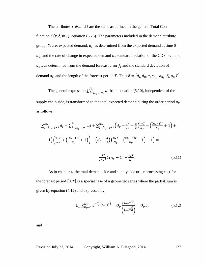
Revision July 23, 2014 Copyright, William A. Ellegood, 2014 127
The attributes are the same as defined in the general Total Cost
function ( ), equation (3.26). The parameters included in the demand attribute
group, , are: expected demand, , as determined from the expected demand at time 0
, and the rate of change in expected demand ; standard deviation of the CDF, and
, as determined from the demand forecast error and the standard deviation of
demand ; and the length of the forecast period . Thus [
].
The general expression ∑
from equation (5.10), independent of the
supply chain side, is transformed to the total expected demand during the order period
as follows
∑
∑
∑ (
)
(
(
( )
)
) (
(
( )
)) (
) (
(
( )
) )
( )
. (5.11)
As in chapter 4, the total demand side and supply side order processing cost for
the forecast period [ ] is a special case of a geometric series where the partial sum is
given by equation (4.12) and expressed by
∑ ( ( ))
( )
(
)
(5.12)
and

128 Copyright, William A. Ellegood, 2014 Revision July 23, 2014
∑ ( ( ))
( )
(
)
. (5.13)
Equation (5.10) is restated following the substitution of equations (5.11), (5.12),
and (5.13) as
( )
( ) [ ∑ ( ( )
(
( ))) ( ( ))
]
( ) [ ∑ ( ( )
(
( )))
( ( )) ]
(5.14)
5.2 Scenario analysis
The baseline supply chain setting considered in Chapter 4 is also used for Chapter
5: the forecast period is 180 days, the lean SCS total production cost to
deliver a single product to the customer is $100, the initial expected demand is 275
units, demand forecast error during the forecast period is constant, the ordering cost
are both $200, and the lean index for the supply side and demand side are
equal, . The values for supply side and demand side lead times and service levels
for each SCS are taken from Table 3.3. Using this baseline supply chain setting, the Total
Cost function for an agile SCS when expected demand is a linear function of time and
demand forecast error is constant for the forecast period is given by

Revision July 23, 2014 Copyright, William A. Ellegood, 2014 129
( )
[ ∑ ( ( )
(
( ))) (
( )
)
]
[ ∑ ( ( )
(
( )))
(( )
) ] . (5.15)
The Total Cost function for an agilean SCS when expected demand is a linear
function of time and demand forecast error is constant for the forecast period is given by
( )
[ ∑ ( ( )
(
( ))) (
( )
)
]
[ ∑ ( ( )
(
( )))
(( )
) ] . (5.16)
The Total Cost function for a leagile SCS when expected demand is a linear
function of time and demand forecast error is constant for the forecast period is given by
( )
[ ∑ ( ( )
(
( ))) (
( )
)
]
[ ∑ ( ( )
(
( )))
(( )
) ] . (5.17)
The Total Cost function for a lean SCS when expected demand is a linear function
of time and demand forecast error is constant for the forecast period is given by

130 Copyright, William A. Ellegood, 2014 Revision July 23, 2014
( )
[ ∑ ( ( )
(
( ))) (
( )
)
]
[ ∑ ( ( )
(
( )))
(( )
) ] . (5.18)
and
for each of the scenarios presented in Figure 3.4 are found by the
complete enumeration of equations (5.15), (5.16), (5.17), and (5.18) for each SCS. The
optimal number of order periods with respect to the SCS are used to determine the Total
Cost values for ( )(
) ( )(
),
( )(
), and ( )(
) when expected demand is a
linear function of time and demand forecast error is constant. The Total Costs for each
SCS are compared and the SCS with the lowest Total Cost for each of the eighty-one
scenarios defined by Figure 3.4 is presented in Figure 5.1.

Revision July 23, 2014 Copyright, William A. Ellegood, 2014 131
Demand Forecast Error
Low
Medium
High
Cost of Capital Cost of Capital Cost of Capital
Low Med. High Low Med. High Low Med. High
Lean
High RMP
High LL LL LL
LL LL LL
LL LL LL
Med. LL LL LL
LL LL LL
LL LL LL
Low LL LA LA
LL LA LA
LL LA LA
Med. RMP
High LL LL AL
LL AL AL
AL AL AL Index Med. LL LL AL
LL LL AL
LL AL AA
Low LA LA AA
LA LA AA
LA AA AA
Low RMP
High AL AL AL
AL AL AA
AL AA AA
Med. LL AA AA
AL AA AA
AA AA AA
Low LA AA AA AA AA AA AA AA AA
Figure 5.1: The SCS with the lowest Total Cost (expected demand and demand forecast
error constant)
From examination of Figure 5.1 some general managerial insights can be
identified. First, a leagile SCS should be considered only when the supply structure is
such that the majority of the production costs are incurred at the supplier (low RMP).
Second, a leagile SCS is the appropriate SCS to minimize Total Cost when the supply
chain structure is such that RMP is low, the lean index is high and the cost of capital is
medium or high, independent of the level of demand forecast error. Third, an agilean SCS
should be considered when the supply chain structure is such that the majority of the
production costs are incurred at the manufacturer (high RMP) and the lean index is either
low or medium. Finally, a supply chain with the following characteristics is very
sensitive to changes in demand forecast error, since it is the only scenario considered
where the SCS that results in the lowest Total Cost changes at each level of demand
Lean SCS
(LL)
Agile SCS
(AA) Leagile SCS
(LA)
Agilean SCS
(AL)

132 Copyright, William A. Ellegood, 2014 Revision July 23, 2014
forecast error considered: low lean index, medium RMP, and the low cost of capital. This
supply chain scenario and others where the appropriate SCS is dependent on the demand
forecast error are examined in greater detail in section 5.3.2.
5.3 Sensitivity analysis
The sensitivity analysis in this chapter focuses on the two aspects of the supply
chain that may be the most uncertain: expected demand and demand forecast error. The
other characteristics examined in this dissertation are likely known with greater certainty
than those associated with expected demand.
The lean index, the ratio of total production cost for an agile SCS to a lean SCS,
will not likely change drastically over a six month period. In those cases where material
pricing could be subject to drastic changes in cost, such as from large changes in raw
material costs or exchange rates, it is assumed that the supply chain will employ the
appropriate financial risk-hedging techniques to mitigate the supply chain’s risk. RMP is
the characteristic considered in this dissertation that the supply chain (or at least the focal
firm of the supply chain) has the greatest control over during the forecast period. Any
changes to the supply chain structure, including RMP, would likely be known several
months, or more, in advance of implementation. Although many aspects of the cost of
capital are outside the control of supply chain members, this research assumes that any
changes in the cost of capital will generally be gradual with respect to time, as could
result when the economies of the nations where supply chain members are located are
relatively stable.
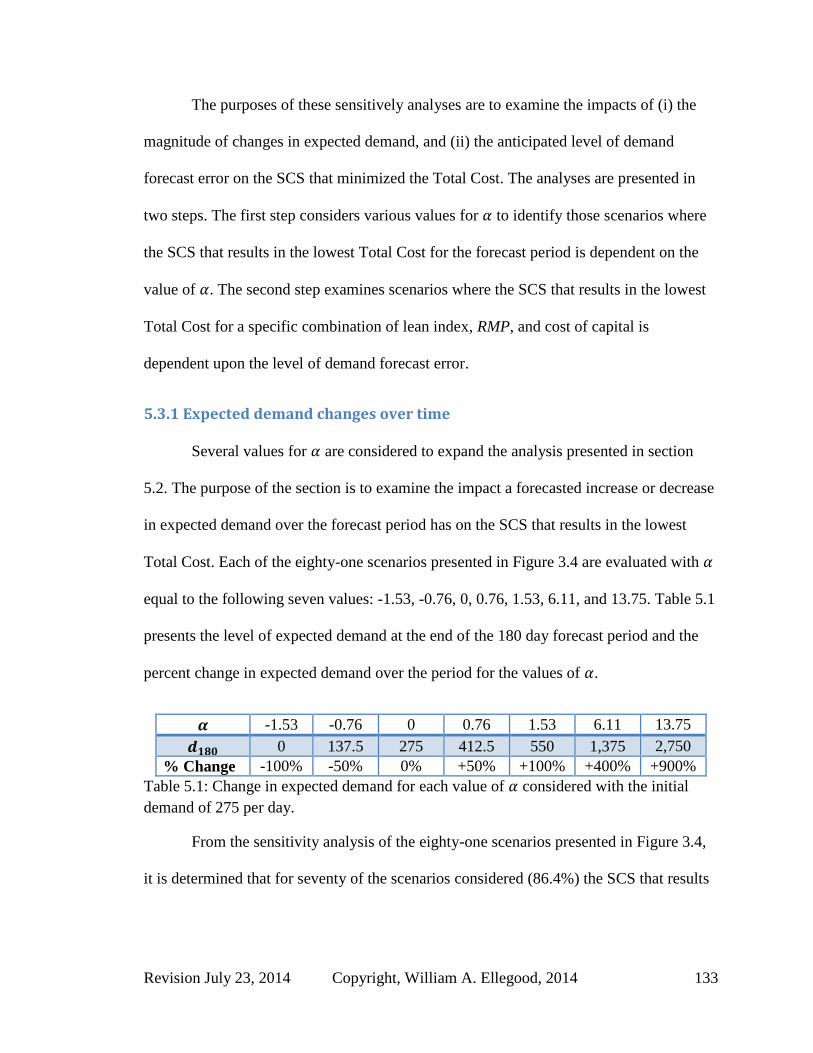
Revision July 23, 2014 Copyright, William A. Ellegood, 2014 133
The purposes of these sensitively analyses are to examine the impacts of (i) the
magnitude of changes in expected demand, and (ii) the anticipated level of demand
forecast error on the SCS that minimized the Total Cost. The analyses are presented in
two steps. The first step considers various values for to identify those scenarios where
the SCS that results in the lowest Total Cost for the forecast period is dependent on the
value of . The second step examines scenarios where the SCS that results in the lowest
Total Cost for a specific combination of lean index, RMP, and cost of capital is
dependent upon the level of demand forecast error.
5.3.1 Expected demand changes over time
Several values for are considered to expand the analysis presented in section
5.2. The purpose of the section is to examine the impact a forecasted increase or decrease
in expected demand over the forecast period has on the SCS that results in the lowest
Total Cost. Each of the eighty-one scenarios presented in Figure 3.4 are evaluated with
equal to the following seven values: -1.53, -0.76, 0, 0.76, 1.53, 6.11, and 13.75. Table 5.1
presents the level of expected demand at the end of the 180 day forecast period and the
percent change in expected demand over the period for the values of .
-1.53 -0.76 0 0.76 1.53 6.11 13.75
0 137.5 275 412.5 550 1,375 2,750
% Change -100% -50% 0% +50% +100% +400% +900%
Table 5.1: Change in expected demand for each value of considered with the initial
demand of 275 per day.
From the sensitivity analysis of the eighty-one scenarios presented in Figure 3.4,
it is determined that for seventy of the scenarios considered (86.4%) the SCS that results

134 Copyright, William A. Ellegood, 2014 Revision July 23, 2014
in the lowest Total Cost is independent of the values of considered. The relative Total
Cost of each SCS to that of the lean SCS is calculated as
( ) ( )
( ). (5.19)
Figures 5.2 and 5.3 illustrate the Total Cost percent difference of the three supply chain
strategies relative to a lean SCS in two settings for the various values of . Figure 5.2
shows that a lean SCS results in the lowest Total Cost independent of the value of for a
supply chain where the scenario is high RMP, high lean index, low demand forecast
error, and low cost of capital. For the scenario presented in Figure 5.2, an agilean SCS is
slightly more expensive than a lean SCS, while an agile SCS and a leagile SCS are over
3% more expensive. Figure 5.3 shows that an agile SCS results in the lowest Total Cost
independent of the value of for a supply chain where the scenario is low RMP, low lean
index, high demand forecast error, and high cost of capital. For the scenario presented in
Figure 5.3, an agilean SCS is nearly 1% more expensive, a leagile SCS is approximately
2% more expensive, and a lean SCS is 2%-3% more expensive than an agile SCS.
In equation (5.19) when the cost ( ) is replaced by ( ),
then computes the cost for an agile SCS relative to a lean SCS. Similarly, when
( ) is replaced by ( ) and ( ), then is the
relative cost of a leagile SCS and an agilean SCS, respectively. When the value of
, a lean SCS results in a lower Total Cost than the comparison SCS; and when
the value of , the comparison SCS results in a lower Total Cost than a lean SCS.

Revision July 23, 2014 Copyright, William A. Ellegood, 2014 135
Figure 5.2: Total Cost of each SCS relative to the Total Cost for a lean SCS with high
RMP, high lean index, low demand forecast error, and low cost of capital.
Figure 5.3: Total Cost of each SCS relative to the Total Cost for a lean SCS with low
RMP, low lean index, high demand forecast error, and high cost of capital.
Figure 5.2 shows a scenario where a lean SCS results in the lowest Total Cost for
the forecast period independent of whether, and how much, demand is (linearly)
increasing or decreasing. In contrast, Figure 5.3 shows a scenario where an agile SCS
0%
1%
2%
3%
4%
-2 0 2 4 6 8 10 12 14
ΦLL
,2
α
agile
leagile
agilean
-3%
-2%
-1%
0%
-2 0 2 4 6 8 10 12 14
ΦLL
,2
α
agile
leagile
agilean

136 Copyright, William A. Ellegood, 2014 Revision July 23, 2014
results in the lowest Total Cost for the forecast period independent of whether, and how
much, demand increases or decreases, for the values of considered.
Figure 5.4 shows the eleven scenarios (parenthetically numbered 1 through 11)
where the SCS that results in the lowest Total Cost is dependent upon the value of . The
other seventy scenarios where the SCS that results in the lowest Total Cost is independent
of the value of , and the corresponding SCS is indicated by the shading in Figure 5.4.
The number in the parentheses denotes the corresponding graph in the following
discussion. The SCS that results in the lowest Total Cost for each of the scenarios when
is given by the background shading in the cell.
Demand Forecast Error
Low
Medium
High
Cost of Capital Cost of Capital Cost of Capital
Low Med. High Low Med. High Low Med. High
Lean
High RMP
High
Med.
Low
Med. RMP
High
(1)
(2)
Index Med.
(9)
Low
(4)
Low RMP
High
(3)
(11) (8)
Med.
(10)
(7)
Low
(5)
(6)
Figure 5.4: Scenarios wehre the lowest cost SCS is dependent upon the value of .
The eleven scenarios are subdivided into four groups based on which supply chain
strategies provide the lowest cost: 1) an agilean SCS or a lean SCS, 2) a leagile SCS or an
Lean SCS
(LL)
Agile SCS
(AA) Leagile SCS
(LA)
Agilean SCS
(AL)

Revision July 23, 2014 Copyright, William A. Ellegood, 2014 137
agile SCS, 3) an agilean SCS or an agile SCS, and 4) an agile SCS, an agilean SCS, or a
lean SCS. For ease of illustration, only those supply chain strategies that result in the
lowest Total Cost for a value of are shown in Figures 5.5, 5.6, 5.7 and 5.8.
RMP-High, -Med., -Med., -Med. RMP-High, -Med., -High, -Med.
RMP-High, -Low, -Med., -Low
Figure 5.5: Group 1: Total Cost of an agilean SCS relative to that of a lean SCS
For all three scenarios depicted in Figure 5.5 a lean SCS results in a lower Total
Cost when is much less than zero. However, for all other values of , an agilean SCS
results in a lower Total Cost than the other three supply chain strategies considered. For
the three scenarios presented in Figure 5.5 where the value of is between -1.5 and 1.5,
the cost difference between a lean SCS and an agilean SCS does not exceed 0.1%.
Therefore, for the values considered here one can conclude (i) using an agilean SCS
-0.10%
-0.05%
0.00%
0.05%
-1.5 -1 -0.5 0 0.5 1 1.5
Φ LL
,2
α
Agilean SCS relative to a Lean SCS
Agilean
-0.10%
-0.05%
0.00%
0.05%
-1.5 -1 -0.5 0 0.5 1 1.5
Φ LL
,2
α
Agilean SCS relative to a Lean SCS
Agilean
-0.10%
-0.05%
0.00%
0.05%
-1.5 -1 -0.5 0 0.5 1 1.5
Φ LL
,2
α
Agilean SCS relative to a Lean SCS
Agilean
(1) (2)
(3)

138 Copyright, William A. Ellegood, 2014 Revision July 23, 2014
and not switching to a lean SCS is at worst 0.03% more expensive and (ii) adopting a
lean SCS is at most 0.1% more expensive than an agilean SCS.
For Figures 5.6 and 5.7, the relative Total Cost of each SCS are determined with
respect to the Total Cost of an agile SCS,
( ) ( )
( ). (5.20)
As in equation (5.19), the cost ( ) in equation (5.20) is replaced by
( ) to determine the value of for a leagile SCS relative to an agile SCS.
Similarly, the cost ( ) is replaced by ( ) to determine for
an agilean SCS. When the value of , an agile SCS results in a lower Total Cost
than the comparison SCS; and when the value of , the comparison SCS results
in a lower Total Cost than an agile SCS.

Revision July 23, 2014 Copyright, William A. Ellegood, 2014 139
RMP-Low, -Med., -High, -Med. RMP-Low, -Low, -Med., -Low
RMP-Low, -Low, -High, -Low
Figure 5.6: Group 2: Total Cost of a leagile SCS relative to that of an agile SCS
For all three scenarios depicted in Figure 5.6 a leagile SCS results in a lower Total
Cost when is less than -1.0 compared to an agile SCS. However, for all larger values of
, an agile SCS results in a lower Total Cost than the other three supply chain strategies.
Furthermore, the financial benefit of adopting a leagile SCS never exceeded 0.6% of the
Total Cost of an agile SCS for the forecast period when the value of is between -1.5
and 1.5. Therefore, unless the cost of changing supply chain strategies is small and the
expected daily demand rate is expected to decrease significantly during the forecast
period, the supply chain should stay with the agile SCS.
-0.4%
-0.2%
0.0%
0.2%
0.4%
0.6%
-1.5 -1 -0.5 0 0.5 1 1.5
ΦA
A,2
α
Leagile SCS relative to an Agile SCS
Leagile
-0.4%
-0.2%
0.0%
0.2%
0.4%
0.6%
-1.5 -1 -0.5 0 0.5 1 1.5
ΦA
A,2
α
Leagile SCS relative to an Agile SCS
Leagile
-0.4%
-0.2%
0.0%
0.2%
0.4%
0.6%
-1.5 -1 -0.5 0 0.5 1 1.5
ΦA
A,2
α
Leagile SCS relative to an Agile SCS
Leagile
(4) (5)
(6)

140 Copyright, William A. Ellegood, 2014 Revision July 23, 2014
RMP-Med., -Low, -High, -Low RMP-High, -Low, -High, -Med.
Figure 5.7: Group 3: Total Cost of an agilean SCS relative to that of an agile SCS
For both scenarios depicted in Figure 5.7, an agilean SCS results in a lower Total
Cost when is approximately -1.25 or less. However, for all other values of , an agile
SCS results in a lower Total Cost than the other three supply chain strategies considered.
Furthermore, the financial benefit of adopting an agilean SCS never exceeds 0.4% of the
Total Cost of an agile SCS. Therefore, unless the cost of changing supply chain strategies
is small and the expected daily demand rate is expected to decrease significantly during
the forecast period, the supply chain should stay with the agile SCS.
-0.4%
-0.2%
0.0%
0.2%
0.4%
-1.5 -1 -0.5 0 0.5 1 1.5
ΦA
A,2
α
Agilean SCS relative to an Agile SCS
Agilean
-0.4%
-0.2%
0.0%
0.2%
0.4%
-1.5 -1 -0.5 0 0.5 1 1.5
ΦA
A,2
α
Agilean SCS relative to an Agile SCS
Agilean
(7) (8)

Revision July 23, 2014 Copyright, William A. Ellegood, 2014 141
RMP-Med., -Med., -High, -Med. RMP-Med., -Low, -Med., -Low
RMP-High., -Low, -High, -Low
Figure 5.8: Group 4: Agile, Agilean SCS vs. Lean SCS
The three scenarios illustrated in Figure 5.8 are the only cases identified where an
greater than zero indicates a change in the SCS results in a lower Total Cost than the
SCS with the lowest Total Cost when . In the upper left graph in Figure 5.8, when
the value is greater than approximately 3.5 an agile SCS results in a lower Total Cost
than an agilean SCS. An value of 3.5 implies the supply chain is expecting a very
significant increase in expected daily demand rate during the forecast period. In the upper
right graph in Figure 5.8, when is approximately 2.5, an agile SCS results in a slightly
lower Total Cost than an agilean SCS. However, an agile SCS results in the lowest Total
Cost for only a small window of values around 2.5. For all other values greater than
approximately an agilean SCS results in a lower Total Cost. The lower graph in
-0.3%
0.0%
0.3%
0.6%
-1.5 -1 -0.5 0 0.5 1 1.5 2 2.5 3 3.5 4
ΦLL
,2
α
Agile SCS, Agilean SCS relative to a Lean SCS
Agile
Agilean
-0.3%
0.0%
0.3%
0.6%
-1.5 -1 -0.5 0 0.5 1 1.5 2 2.5 3 3.5 4
ΦLL
,2
α
Agile SCS, Agilean SCS relative to a Lean SCS
Agile
Agilean
-0.3%
0.0%
0.3%
0.6%
-1.5 -1 -0.5 0 0.5 1 1.5 2
ΦLL
,2
α
Agile SCS, Agilean SCS relative to a Lean SCS
Agile
Agilean
(9) (10
)
(11
)

142 Copyright, William A. Ellegood, 2014 Revision July 23, 2014
Figure 5.8 is the only scenario where a change in the lowest cost SCS from the best SCS
when expected daily demand rate is held constant for the forecast period ( ) occurs
with an value between -1.0 and 1.5. In this example, if the supply chain is anticipating
the expected daily demand rate to increase more than 25% ( ) during the forecast
period, then an agile SCS should be adopted to minimize the Total Cost.
5.3.2 Demand forecast error and demand changes with time
Figure 5.9 shows the twenty-seven scenarios where the the SCS that results in the
lowest Total Cost is dependent upon the demand forecast error value. Often it is difficult
to accurately forecast expected demand and the level of uncertainty associated with the
forecast. For example, Hewlett-Packard in the 1990’s found that the level of demand
forecast error for a printer during its introduction stage was 80-90% and the demand
forecast error improved to around 40% during the maturity stage of a printer’s life cycle
(Simchi-Levi et al., 2008, pg. 362). In Figure 5.9, the twenty-seven scenarios where the
SCS that results in the lowest Total Cost depends on the magnitude of demand forecast
error are noted by the two letter abbreviation of the SCS.

Revision July 23, 2014 Copyright, William A. Ellegood, 2014 143
Demand Forecast Error
Low
Medium
High
Cost of Capital Cost of Capital Cost of Capital
Low Med. High Low Med. High Low Med. High
Lean
High RMP
High
Med.
Low
Med. RMP
High LL LL
LL AL
AL AL
Index Med.
LL AL
LL AL
AL AA
Low
LA
LA
AA
Low RMP
High
AL AL
AL AA
AA AA
Med. LL
AL
AA
Low LA
AA
AA
Figure 5.9: SCS was dependent upon the demand forecast error value
The twenty-seven scenarios in Figure 5.9 are partitioned into six categories
(identified by a number in parenthesis to the right of Figure 5.9) based on the lean index
and RMP value: 1) RMP high and lean index medium, 2) RMP medium and lean index
medium, 3) RMP low and lean index medium, 4) RMP high and lean index low, 5) RMP
low and lean index low, and 6) RMP medium and lean index low. Figures 5.10 through
5.15 illustrates the Total Cost relative to either a lean SCS or an agile SCS, accordingly,
with respect to the level of demand forecast error and the anticipated change in expected
daily demand rate during the forecast period, .
LL-Lean SCS AA-Agile SCS LA-Leagile SCS AL-Agilean SCS
(1)
(2)
(3)
(4)
(6)
(5)

144 Copyright, William A. Ellegood, 2014 Revision July 23, 2014
RMP-High, -Medium, -Low
RMP-High, -Medium, -Medium
Figure 5.10: Category 1 - RMP-High and Lean Index Medium
For Category 1, with low cost of capital (top of Figure 5.10), a lean SCS results in
the lowest Total Cost for supply chains where the demand forecast error is less than 80%
and when the value of is less than approximately 0.70. However, with low cost of
capital, when demand forecast error is >80%, and expected daily demand rate is stable or
is expected to increase, the supply chain should consider adopting an agilean SCS to
minimize Total Cost. With the cost of capital at a medium level (bottom of Figure 5.10)
-0.2%
-0.1%
0.0%
0.1%
0.2%
0.3%
-1.5 -1.0 -0.5 0.0 0.5 1.0 1.5
ΦLL
,2
α
Agilean SCS relative to a Lean SCS
0%
20%
40%
60%
80%
100%
Demand Forecast
Error
-0.2%
-0.1%
0.0%
0.1%
0.2%
0.3%
-1.5 -1.0 -0.5 0.0 0.5 1.0 1.5
ΦLL
,2
α
Agilean SCS relative to a Lean SCS
0%
20%
40%
60%
80%
100%
Demand Forecast
Error

Revision July 23, 2014 Copyright, William A. Ellegood, 2014 145
the supply chain should adopt a lean SCS when demand forecast error is less than 20% or
the expected daily demand rate decreases significantly during the forecast period;
otherwise the supply chain should employ an agilean SCS.
RMP-Medium, -Medium, -Medium
RMP-Medium, -Medium, -High
Figure 5.11: Category 2 - RMP-medium and lean index medium
For Category 2, with medium cost of capital (top of Figure 5.11), a lean SCS
should be adopted when demand forecast error is 40% or less or when the expected daily
demand rate is anticipated to decrease significantly. However, when the demand forecast
-0.3%
-0.1%
0.1%
0.3%
-1.5 -1.0 -0.5 0.0 0.5 1.0 1.5
ΦLL
,2
α
Agilean SCS relative to a Lean SCS
0%
20%
40%
60%
80%
100%
Demand Forecast
Error
-0.3%
-0.1%
0.1%
0.3%
-1.5 -1.0 -0.5 0.0 0.5 1.0 1.5
ΦA
A,2
α
Agilean SCS relative to an Agile SCS
100%
80%
60%
40%
20%
0%
Demand Forecast
Error

146 Copyright, William A. Ellegood, 2014 Revision July 23, 2014
error is greater than 40% and the level of expected daily demand rate is stable or
increasing for the forecast period, then the supply chain should adopt an agilean SCS.
When the cost of capital is at a high level (bottom of Figure 5.11), the supply chain
should adopt an agile SCS when demand forecast error is greater than 40% and the
expected daily demand rate is stable or increasing; otherwise the supply chain should
consider adopting an agilean SCS.
RMP-Low, -Medium, -Medium
Figure 5.12: Category 3 - RMP-low and lean index medium
For Category 3, Figure 5.12 shows that an agile SCS should be employed when
the demand forecast error is greater than 60% and the expected daily demand rate is
nearly stable or increasing, and a leagile SCS should be adopted when the demand
forecast error is less than 60% or when the expected daily demand rate decreases
significantly during the forecast period.
-0.5%
-0.3%
-0.1%
0.1%
0.3%
-1.50 -1.00 -0.50 0.00 0.50 1.00 1.50
ΦA
A,2
α
Leagile SCS relative to an Agile SCS
100%
80%
60%
40%
20%
0%
Demand Forecast
Error
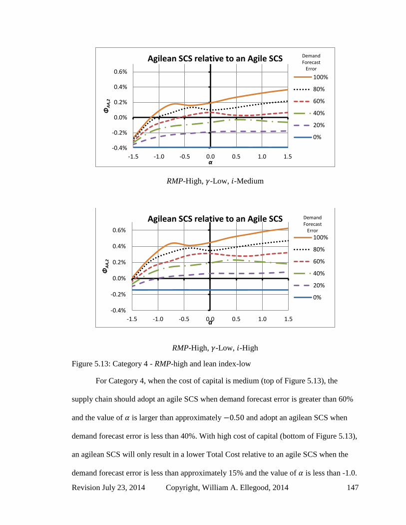
Revision July 23, 2014 Copyright, William A. Ellegood, 2014 147
RMP-High, -Low, -Medium
RMP-High, -Low, -High
Figure 5.13: Category 4 - RMP-high and lean index-low
For Category 4, when the cost of capital is medium (top of Figure 5.13), the
supply chain should adopt an agile SCS when demand forecast error is greater than 60%
and the value of is larger than approximately and adopt an agilean SCS when
demand forecast error is less than 40%. With high cost of capital (bottom of Figure 5.13),
an agilean SCS will only result in a lower Total Cost relative to an agile SCS when the
demand forecast error is less than approximately 15% and the value of is less than -1.0.
-0.4%
-0.2%
0.0%
0.2%
0.4%
0.6%
-1.5 -1.0 -0.5 0.0 0.5 1.0 1.5
ΦA
A,2
α
Agilean SCS relative to an Agile SCS
100%
80%
60%
40%
20%
0%
Demand Forecast
Error
-0.4%
-0.2%
0.0%
0.2%
0.4%
0.6%
-1.5 -1.0 -0.5 0.0 0.5 1.0 1.5
ΦA
A,2
α
Agilean SCS relative to an Agile SCS
100%
80%
60%
40%
20%
0%
Demand Forecast
Error

148 Copyright, William A. Ellegood, 2014 Revision July 23, 2014
RMP-Low, -Low, -Low
Figure 5.14: Category 5 - RMP-low and lean index-low
For Category 5, illustrated in Figure 5.14 (low RMP, low lean index, and low cost
of capital), the supply chain should adopt an agile SCS when demand forecast error is
greater than approximately 20% and the value of is larger than 0, and a leagile SCS
when demand forecast error is less than 20%. Otherwise, the SCS that results in the
lowest Total Cost, either leagile SCS or agile SCS, is dependent on the value of demand
forecast error and the value of .
-0.3%
-0.1%
0.1%
0.3%
0.5%
-1.5 -1.0 -0.5 0.0 0.5 1.0 1.5
ΦA
A,2
α
Leagile SCS relative to an Agile SCS
100%
80%
60%
40%
20%
0%
Demand Forecast
Error
-0.4%
-0.2%
0.0%
0.2%
-1.5 -1.0 -0.5 0.0 0.5 1.0 1.5
ΦLL
,2
α
Agliean SCS relative to a Lean SCS
0%
20%
40%
60%
80%
100%
Demand Forecast
Error

Revision July 23, 2014 Copyright, William A. Ellegood, 2014 149
RMP-Medium, -Low, -Low
Figure 5.15: Category 6 - RMP-medium and lean index-low
Finally, Category 6 depicted in Figure 5.15 (medium RMP, low lean index, and
low cost of capital), includes the only scenarios examined where the SCS that results in
the lowest Total Cost is different at all three levels of demand forecast error considered in
Figure 3.4. When the expected demand forecast error increases from low to medium the
SCS which minimizes Total Cost changes from lean SCS to an agilean SCS, and then
when the expected demand forecast error increases to a high level the SCS that minimizes
Total Cost is an agile SCS. From Figure 5.15, a lean SCS minimizes Total Cost when
demand forecast error is approximately 18% or less, independent of the value of . An
agilean SCS should be implemented when the demand forecast error ranges from
approximately 18% to 40% and the value of is greater than -1.0. An agile SCS should
be adopted when the demand forecast error is greater than 60% and the value of is
greater than -0.75. The SCS that results in the lowest Total Cost for those supply chains
with medium RMP, low lean index, low cost of capital, and when the level of demand
-0.4%
-0.2%
0.0%
0.2%
-1.5 -1.0 -0.5 0.0 0.5 1.0 1.5
ΦA
A,2
α
Agilean SCS relative to an Agile SCS
100%
80%
60%
40%
20%
0%
Demand Forecast
Error

150 Copyright, William A. Ellegood, 2014 Revision July 23, 2014
forecast error and the value of are not one of the three combinations presented, needs to
be evaluated on a case by case basis.
5.4 Summary
The two purposes of this chapter were to determine the SCS that resulted in the
lowest Total Cost for the various scenarios considered and to examine the sensitivity of
the lowest cost SCS selected to changes in aspects of expected demand. Figure 5.16
expands the cubes from Figure 3.4 and identifies the appropriate SCS that minimizes
Total Cost for each scenario, assuming the baseline supply chain setting presented in
Chapter 4. From Figure 5.16, a leagile SCS should be considered when the structure of
the supply chain is such that the vast majority of production costs are incurred at the
supplier (low RMP) and an agilean SCS should be considered when the structure of the
supply chain is such that the majority of production costs are incurred at the manufacturer
(high RMP) and lean index is low or medium.

Revision July 23, 2014 Copyright, William A. Ellegood, 2014 151
Figure 5.16: The SCS which results in the lowest Total Cost for all scenarios considered.
The sensitivity analysis of SCS selection with respect to an anticipated increase or
decrease in expected demand during the forecast period shows that for the majority of
scenarios considered (86.4%) the SCS that results in the lowest Total Cost is independent
of a change in the expected demand level during the forecast period. For each of the
groups where the SCS that results in the lowest Total Cost is dependent on the anticipated
change in expected daily demand rate during the forecast period, when a considerable
decrease in expected demand is anticipated a leaner SCS may result in a lower Total
Cost. For example, scenarios in Group 1 would move from an agilean SCS to a lean SCS,
Group 2 would move from an agile SCS to a leagile SCS, Group 3 would move from an
agile SCS to an agilean SCS, and Group 4 would move from an agilean SCS to a lean
SCS. The analysis shows that generally the appropriate SCS to minimize Total Cost when
RMP
Low
High
RMP
Low
High
RMP
Low
High
Cost of
Capital
Low High Cost of
Capital
Low High Cost of
Capital
Low High
Demand Forecast
Error—Low
Lean Index
Low
Lean Index
Medium
Lean Index
High
Demand Forecast
Error—Medium
Demand Forecast
Error—High Agile SCS
Lean SCS
Leagile SCS
Agilean
152 Copyright, William A. Ellegood, 2014 Revision July 23, 2014
the anticipated change in expected daily demand rate over the forecast period is between -
50% to +100% is the same as when expected daily demand rate is constant for the
forecast period; therefore, the simpler model presented in Chapter 4 might be sufficient
for determining the SCS that minimizes Total Cost for the supply chain. The single
scenario where the SCS that results in the lowest Total Cost changes when the change in
expected daily demand rate is between -50% to +100% occurs with high RMP, low lean
index, low cost of capital and high demand forecast error, the cube shaded by diagonal
lines in Figure 5.16. This analysis assumes the initial expected demand is 275 units per
day and further analysis would be needed to determine the range of demand values where
these findings are generalizable.
The analysis of the sensitivity of the lowest Total Cost SCS for the forecast
period with respect to the level of demand forecast error shows that when the lean index
is high, the lowest cost SCS is independent of the demand forecast error level. When the
lean index and the cost of capital are both medium, the SCS that results in the lowest
Total Cost is dependent on the demand forecast error level for the values of RMP
considered here. For the scenarios with low lean index, medium RMP, and the low cost of
capital, shown by the cubes shaded by horizontal lines in Figure 5.16, the SCS that results
in the lowest Total Cost changes at each level of demand forecast error considered.

Revision July 23, 2014 Copyright, William A. Ellegood, 2014 153
6. Supply chain strategy selection for product life cycle
The question addressed by this chapter is Q3: Under what combination of supply
chain characteristics does each SCS minimize total supply chain cost over the life cycle
of a product?
This chapter uses the term “simple SCS” to denote the situation where the SCS is
not allowed to change over the PLC. The term “complex SCS” is used to denote the
situation where the SCS is allowed to change during the PLC. For some scenarios where
the SCS does not change over the PLC, the complex SCS is the same as the simple SCS.
The primary purpose of this chapter is to (i) determine which SCS results in the lowest
Total Cost over the product life cycle when the SCS does not change over the PLC
(simple SCS), and (ii) determine the impact on the Total Cost of using a simple SCS
versus allowing the SCS to change during the PLC (complex SCS).
6.1 Problem description
The classical PLC, shown in Figure 6.1, includes four stages: introduction,
growth, maturity, and decline. For products in the introduction stage of the PLC there is a
high level of uncertainty associated with the expected market response and the diffusion
rate of the product in the market, which results in a low level of demand predictability
and a high level of demand forecast error. In the growth stage, products experience an
increase in unit sales per time period but at a diminishing rate as competing products
eventually enter the market and the saturation level of the product in the market
increases. At the maturity stage of the PLC, the demand rate is at its highest level and the

154 Copyright, William A. Ellegood, 2014 Revision July 23, 2014
predictability of demand has improved resulting in a lower level of demand forecast
error.
Figure 6.1: Classical product life cycle (Source: Rink and Swan, 1979)
The literature does not include a general function for the classical PLC model;
however, the PLC can be modeled as a 4th
degree polynomial. For this dissertation, the
following assumptions are made concerning the classical PLC function: (i) it describes
the expected demand as a function of time, ( ), (ii) the PLC is a 4th
degree polynomial,
(iii) the function intersects the horizontal axis in exactly two places, at and ,
and (iv) no point along the function lies below the horizontal axis, ( ) [ ]
. The general expression for the PLC is then
( )
, (6.1)
and with the assumptions from the previous paragraph, the PLC may be further simplified
to
( ) √
. (6.2)
Unit Sales
Introduction Growth Maturity Decline Time 0
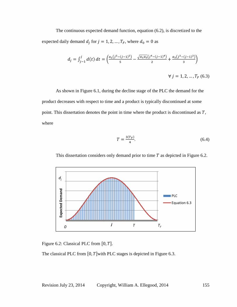
Revision July 23, 2014 Copyright, William A. Ellegood, 2014 155
The continuous expected demand function, equation (6.2), is discretized to the
expected daily demand for , where as
∫ ( )
(
( ( ) )
√ ( ( ) )
( ( ) )
)
(6.3)
As shown in Figure 6.1, during the decline stage of the PLC the demand for the
product decreases with respect to time and a product is typically discontinued at some
point. This dissertation denotes the point in time where the product is discontinued as ,
where
( )
. (6.4)
This dissertation considers only demand prior to time as depicted in Figure 6.2.
Figure 6.2: Classical PLC from [ ].
The classical PLC from [ ]with PLC stages is depicted in Figure 6.3.
Exp
ect
ed
De
man
d
j
PLC
Equation 6.3
TF 0
dj
T

156 Copyright, William A. Ellegood, 2014 Revision July 23, 2014
Figure 6.3: Classical PLC from [ ] with PLC stages.
For a given total expected demand for a product, , over the PLC [ ], the
values of and are determined by setting equation (6.2) equal to zero and solving for
:
( ) ,
√
√ (6.5)
or, using equation 6.4,
. (6.6)
The parameter can be expressed in terms of total expected demand over the PLC, ,
and the length of the PLC, , by substituting equation (6.6) into equation (6.2) and
solving the following expression
∫
dj
Introduction Growth Maturity Decline T 0 j

Revision July 23, 2014 Copyright, William A. Ellegood, 2014 157
(
)
. (6.7)
The expected daily demand in terms of total expected demand, , and the length of
the PLC, , is determined by substituting equations (6.6) and (6.7) into equation (6.3),
( ( ( ) )
( ( ) )
( ( ) )
). (6.8)
This research assumes that the PLC is subdivided into nonoverlapping
sequential time periods, denoted as epochs, and each epoch is in length, so that
. (6.9)
The modification of the Total Cost function employed in this chapter to determine the
Total Cost over the life-cycle of a product employs a rolling horizon perspective. A
rolling horizon perspective invokes a solution method where an initial solution is
determined for the first epoch of the PLC (starting at time 0). The ending position from
the initial epoch is then used to determine the optimal solution to the next epoch of the
PLC. This process is repeated until a solution had been determined for all epochs of the
PLC.
The rolling horizon heuristic allows the number of order periods to vary between
epochs and thus to change over the PLC. With a simple SCS, the same SCS is used for all
epochs of the PLC, the supply side and the demand side service levels and lead times are
constant for all epochs of the PLC, but the number of order periods per epoch may differ

158 Copyright, William A. Ellegood, 2014 Revision July 23, 2014
between epochs of the PLC. With a complex SCS, the SCS may change during the PLC,
so the supply side and demand side service levels and lead times which are dependent on
the SCS selected for each epoch may differ between epochs of the PLC. With a complex
SCS, the number of supply side and demand side order periods may also differ between
epochs.
The epochs of the PLC are indexed by . The number of demand
side order periods for an epoch of the PLC is denoted by . Similarly, for the supply
side the number of order periods for an epoch of the PLC is denoted by . The set of
possible values for is taken as a positive integer [ ], such that
is an integer.
Therefore, the minimum value for is 1 and the maximum value for
is . The set
of possible values for is defined similarly so that
is an integer. The individual
demand side orders for epoch are indexed by and the individual
supply side orders for epoch are indexed by . When is large, the
set of possible values for and may include many values. For example, when
the set includes { }. Order of epoch is
for the expected demand plus safety stock requirements for the order period from day
( ) to , where
is given by
(
). (6.10)
Order of epoch will arrive at the customer at time ( ). The length of each order
period of epoch is

Revision July 23, 2014 Copyright, William A. Ellegood, 2014 159
. (6.11)
The demand side costs of order of epoch are incurred at time
( ) . (6.12)
Similarly, order of epoch is the expected demand plus safety stock
requirements for the order period from time ( ) to , where
is given by
(
). (6.13)
Order arrives at the customer at time ( ). The length of each order period of
epoch is
. (6.14)
The supply side costs of order of epoch are incurred at time
( ) . (6.15)
As Rinker (1979) discussed, the demand variability of a product that exhibited the
classical PLC tends to reduce with time. To capture this aspect of the classical PLC,
demand forecast error is modeled as an exponential decay function of time,
( )
. (6.16)
The parameter in equation (6.16) is a decay factor that allows the impact of the
rate at which demand variability decreases over the PLC to be examined. To determine

160 Copyright, William A. Ellegood, 2014 Revision July 23, 2014
the value of coefficients and in equation (6.16), this dissertation assumes that the
initial value for demand forecast error at time zero is known and that the demand forecast
error at time is zero. The values of and are determined by solving equation (6.6)
for ( ) and ( ) simultaneously, where ( )
and ( ) (
). The
resulting decay function for demand forecast error for the forecast period [ ],
expressed in terms of the demand forecast error at time zero and the length of the PLC,
where ( ) and , is
( ) ( ) (
). (6.17)
The demand forecast error function is discretized in terms of days from 0 to ,
where ( ) and
∫ ( )
(
(
( )
) (
)
( )). (6.18)
Realized demand is assumed to be normally distributed about expected demand
for the life cycle of the product; [ ( ( )) ]. Expected demand, realized demand
and the demand forecast error are presumed constant for each day and the expected
daily demands are assumed mutually independent. The standard deviation of realized
demand about expected demand is defined by substituting equations (6.8) and (6.18) into
equation (3.15),
. (6.19)

Revision July 23, 2014 Copyright, William A. Ellegood, 2014 161
The standard deviation of the cumulative distribution function (CDF) of expected
demand for each order period is the square root of the summation of the expected demand
variances for the entire order period. The CDF for the demand side of the supply chain is
determined by
√∑
( ) .
(6.20)
The CDF for the supply side of the supply chain is determined by
√∑
( ) .
(6.21)
The safety stock inventory levels for each order period, , of epoch
with supply chain strategy are
(6.22)
and
. (6.23)
The demand side safety stock inventory level at the start of the initial epoch of the
PLC, where and , is assumed to be zero, and is given by
(6.24)
For subsequent epochs of the PLC, the demand side initial safety stock inventory
level of the epoch, for and , is the expected safety stock inventory level of
the last order period of the previous epoch, given by
162 Copyright, William A. Ellegood, 2014 Revision July 23, 2014
( )
( ) ( ). (6.25)
The supply side safety stock inventory level at the start of the initial epoch of the
PLC, where and , is assumed to be zero, and is given by
(6.26)
For subsequent epochs of the PLC, the supply side safety stock inventory level at
the beginning of each epoch, when and , is the safety stock inventory level
of the last order period of the previous epoch, given by
( )
( ) ( ). (6.27)
The safety stock inventory ordered in each order period is the difference between
the safety stock inventory level of the current order period and the previous order period.
The change in safety stock inventory level from the previous order period to the next
order period for the demand side is
( ). (6.28)
The change in safety stock inventory level from the previous order period to the
next order period for the supply side is
( ). (6.29)
The PLC Total Cost function when expected demand mimics a classical PLC and
demand forecast error improves with time, denoted ( ), is the summation of the
Total Cost for each epoch of the PLC. The PLC Total Cost for a complex SCS is

Revision July 23, 2014 Copyright, William A. Ellegood, 2014 163
developed by substituting equations (6.3), (6.28), and (6.29) into equation (3.32) and
summing over all epochs,
( )
( ) ∑ [∑ ( {(∑
( )
)
( )} )
( ( ))
]
( ) [∑ ( {(∑
( )
)
( )} )
( ( ))].
(6.30)
The attributes are the same as defined in the general Total Cost
function ( ), equation (3.26). The parameters included in the attribute group, ,
when expected demand mimics a classical PLC and demand forecast error improves with
time during the PLC are: expected demand , as determined from the total expected
demand and the parameter ; the standard deviation of the CDF for epoch ,
and , as determined from the demand forecast error and the standard deviation of
demand ; the length of each epoch ; and the length of the PLC . Thus
[
].
As in chapter 4, the total demand side and supply side order processing cost for
each epoch of the PLC is a special case of a geometric series where the partial sum is
given by equation (4.12) and expressed by
∑ ∑ ( ( ))
∑
( )
(
)
( ) (6.31)

164 Copyright, William A. Ellegood, 2014 Revision July 23, 2014
and
∑ ∑ ( ( ))
∑
( )
(
)
( ) . (6.32)
Let
( )
(
)
and
( )
(
)
.
Equations (6.31) and (6.32) are substituted into equation (6.30); therefore, the PLC Total
Cost for a complex SCS is
( )
( ) ∑ [∑ ( {(∑
( )
)
( )})
( ( ))
( )
]
( ) [∑ ( {(∑
( )
)
( )})
( ( ))
( )
]. (6.33)
6.2 Scenario analysis
To identify the SCS which minimizes Total Cost over the life cycle of a product,
the scenario analysis considers the combinations of three PLC lengths (1 year, 2 years,
and 5 years) and two values for total expected demands (100,000 and 1,000,000 units) for
a total of six product situations. It is assumed the length of each epoch of the PLC is
days and each year has 360 days. As in chapters 4 and 5, the lean SCS total
production cost to deliver a single product to the customer is $100, the ordering

Revision July 23, 2014 Copyright, William A. Ellegood, 2014 165
cost are both $200, and the lean index for the supply side and demand side are
equal, . The demand forecast error is assumed to improve over the course of the
PLC following equation (6.18) and the parameters used to describe the low, medium, and
high levels are based on values of demand forecast error for a functional and an
innovative product from Fisher (1997), given in Table 6.1.
Demand Characteristics Functional Innovative
Product life cycle >= 2 years 3 months to 1 year
Contribution margin 5% to 20% 20% to 60%
Product variety Few Many
Average forecast error 10% 40% to 100%
Average stockout 1% to 2% 10% to 40%
Quantity sold at discount 0% 10% to 25%
Lead time for made to
order
6 months to 1 year 1 day to 2 weeks
Source: Fisher, 1997
Table 6.1: Characteristics of functional and innovative products:
Fisher (1997) expressed that the average demand forecast error of a functional
product was less than 10%, and for an innovative product was between 40% and 100%.
This dissertation defines three levels of demand forecast error as follows: a high level of
demand forecast error is where the demand forecast error is initially 100% and improves
to 40% when expected demand is at its highest; a medium level of demand forecast error
assumes demand forecast error is initially 100% and improves to 10% when expected
demand is at its highest; and a low level of demand forecast error is where the demand
forecast error is initially 40% and when expected demand is at its highest the demand
forecast error improves to 10%. An illustration of the three levels of demand forecast
error and expected demand with respect to time is given in Figure 6.4. Figure 6.5

166 Copyright, William A. Ellegood, 2014 Revision July 23, 2014
illustrates for the three levels of demand forecast error with respect to day
over the PLC.
Figure 6.4: Demand forecast error and expected demand with respect to time.
Figure 6.5: for each level of demand forecast error with respect to time.
The values defined as low, medium, and high levels for RMP, lean index, and cost
of capital are the same as in the previous chapters, and are shown in Table 6.2. The
assumed values for demand forecast error are also given in Table 6.2.
0%
10%
20%
30%
40%
50%
60%
70%
80%
90%
100%
110% dj fj
j
Levels of Demand Forecast Error
High
Medium
Low
ExpectedDemand
T
0
50
100
150
200
250
300
350
dj
j
Levels of Demand Forecast Error
Upper High
Upper Med
Upper Low
Expected Demand
Lower Low
Lower Med
Lower High
T
Revision July 23, 2014 Copyright, William A. Ellegood, 2014 167

168 Copyright, William A. Ellegood, 2014 Revision July 23, 2014
Characteristics Low Medium High
RMP ( ⁄ ) 1/9 1 9
Cost of Capital ( ) .01389% .02778% .04167%
Lean Index ( ) 1.01 1.02 1.04
Initial Forecast Error ( ) 40% 100% 100%
Forecast Error at Maximum
Demand ( ⁄ ) 10% 10% 40%
Table 6.2: Values for characteristics considered in Chapter 6.
The lowest PLC Total Cost for each simple SCS and the complex SCS is
determined as follow: the first epoch of the PLC is enumerated for each SCS model to
identify the optimal number of orders
and
for each SCS. This process is then
repeated for each SCS and each epoch of the PLC until the values of
and
for
all epochs of each SCS has been determined. The PLC Total Cost for each simple SCS
and the complex SCS is the summation of the (discounted) Total Cost for each epoch for
the PLC.
The research considers four types of simple supply chain strategies (lean, agile,
leagile, and agilean). For each of the simple supply chain strategies, the SCS is constant
for each epoch of the PLC. For example, with a simple lean SCS the optimal number of
orders and the Total Cost of each epoch of the PLC are determined assuming a lean SCS.
For the complex SCS, all four SCS types are considered for each epoch of the PLC.
Therefore, for a PLC with twenty epochs, the SCS could switch many times over the
PLC.
With a lean supply side strategy, for most products it seems unrealistic for a firm
planning the SCS of a product over its life-cycle, which could be several years in length,
to plan to place frequent (e.g., daily) orders sixty days in advance of when the expected

Revision July 23, 2014 Copyright, William A. Ellegood, 2014 169
demand will be realized. Further, in part, the cost advantage achieved by a lean SCS
results from economies of scale and for many products economies of scale cannot be
realized when shipping daily. For these reasons when a lean supply side strategy is
considered the model limits
. Therefore, when the supply side strategy is a lean
strategy, the frequency that supply side orders can be placed is no more than
approximately once every two weeks. Similarly, with a lean demand side strategy the
model limits
. Hence, with a demand side lean strategy the frequency that
demand side orders can be placed is no more than once every six days or approximately
once per week.
The values for supply side and demand side lead times and service levels for each
simple SCS are taken from Table 3.3 and are presented in Table 6.3.
Agile Agilean Leagile Lean
Supply Side
Purchased
Material Cost
=1.280 =1.280 =2.055 =2.055
(days)
Demand
Side
Manufacturing
Cost
=1.280 =2.055 =1.280 =2.055
(days)
Table 6.3: Time and cost variables for a lean, leagile, and agile supply chain

170 Copyright, William A. Ellegood, 2014 Revision July 23, 2014
The PLC Total Cost function for a simple agile SCS is
( )
∑ [∑ ( {(∑
( ) ) ( ( ))})
( ( )) ( )
]
[∑ ( ( ) {(∑
( ) ) ( ( ))})
( ( ))
( )].
(6.34)
The PLC Total Cost function for a simple agilean SCS is
( )
∑ [∑ ( {(∑
( ) ) ( ( ))})
( ( )) ( )
]
[∑ (( ) {(∑
( ) ) (
( ))})
( ( ))
( )].
(6.35)
The PLC Total Cost function for a simple leagile SCS is
( )
∑ [∑ ( {(∑
( ) ) ( ( ))})
( ( )) ( )
]
[∑ ( ( ) {(∑
( ) ) ( ( ))})
( ( ))
( )].
(6.36)

Revision July 23, 2014 Copyright, William A. Ellegood, 2014 171
The PLC Total Cost function for a simple lean SCS is
( )
∑ [∑ ( {(∑
( ) ) (
( ))}) ( ( ))
( )
]
[∑ (( ) {(∑
( ) ) ( ( ))})
( ( ))
( )].
(6.37)
and
for each epoch of each of each scenario presented in Figure 3.4 and
the product situation combination for each SCS are found by the complete enumeration
of equations (6.34), (6.35), (6.36), and (6.37). The optimal number of order periods for
each epoch with respect to the SCS are used to determine the Total Cost values for
( ) ( ), ( ), and ( ) when expected
demand mimics the classical PLC and demand forecast error improves with time. Figures
6.6-6.11 shows the simple SCS that results in the lowest PLC Total Cost for each of the
scenarios presented in Table 6.1 for the six situations considered ( 100,000 or
1,000,000 units, and 1 year, 2 years, or 5 years). Out of the 486 scenarios considered
(81*6) there are only three instances (0.6%) where the complex SCS resulted in a lower
PLC Total Cost than a simple SCS. These three cases all occur when the PLC length is 5
years and the total expected demand is 100,000 units. The cases where the complex SCS
results in a lower PLC Total Cost are noted in Figure 6.6 by the cells shaded with
diagonal lines. The legend for Figures 6.6-6.11 is shown with Figure 6.6.

172 Copyright, William A. Ellegood, 2014 Revision July 23, 2014
5 years 100,000 units Demand Forecast Error
Low Medium High
Cost of Capital Cost of Capital Cost of Capital
Low Med High Low Med High Low Med High
Lean
High RMP
High LL LL LL
LL LL LL
LL LL LL
Med LL LL LL
LL LL LL
LL LL LL
Low LL LA LA
LL LA LA
LL LA LA
Med RMP
High LL LL AL
LL LL AL
LL LL AL
Index Med LL LL AL
LL LL AL
LL LL LL
Low LA LA AA
LA LA AA
LA LA LA
Low RMP
High AL AL AL
AL AL AL
LL AL AL
Med LL AA AA
AA AA AA
LL AA AA
Low LA AA AA
LA AA AA
LA AA AA
Figure 6.6: The simple SCS that results in the lowest PLC Total Cost when =100,000
and 5 years for each scenario.
5 years. 1,000,000 units Demand Forecast Error
Low Medium High
Cost of Capital Cost of Capital Cost of Capital
Low Med High Low Med High Low Med High
Lean
High RMP
High LL LL LL
LL LL LL
LL LL LL
Med LL LL LL
LL LL LL
LL LL LL
Low LL LA LA
LL LA LA
LL LA LA
Med RMP
High LL LL AL
LL LL AL
LL LL LL
Index Med LL LL AL
LL LL AL
LL LL AL
Low LA LA AA
LA LA AA
LA LA AA
Low RMP
High LL AL AL
LL AL AA
LL AL AL
Med LL AL AA
LL AL AA
LL AL AA
Low LA AA AA
LA AA AA
LA AA AA
Figure 6.7: The simple SCS that results in the lowest PLC Total Cost when
=1,000,000 and 5 years for each scenario.
Lean SCS
LL
Agile SCS
AA
Leagile SCS
LA
Agilean SCS
AL

Revision July 23, 2014 Copyright, William A. Ellegood, 2014 173
2 years 100,000 units Demand Forecast Error
Low Medium High
Cost of Capital Cost of Capital Cost of Capital
Low Med High Low Med High Low Med High
Lean
High RMP
High LL LL LL
LL LL LL
LL LL LL
Med LL LL LL
LL LL LL
LL LL LL
Low LL LA LA
LL LA LA
LL LA LA
Med RMP
High LL LL AL
LL LL AL
LL LL LL
Index Med LL LL AL
LL LL AL
LL LL AL
Low LA LA AA
LA LA AA
LA LA AA
Low RMP
High LL AL AL
LL AL AL
LL AL AL
Med LL AA AA
LL AA AA
LL AL AA
Low LA AA AA
LA AA AA
LA AA AA
Figure 6.8: The simple SCS that results in the lowest PLC Total Cost when =100,000
and 2 years for each scenario.
2 years 1,000,000 units Demand Forecast Error
Low Medium High
Cost of Capital Cost of Capital Cost of Capital
Low Med High Low Med High Low Med High
Lean
High RMP
High LL LL LL
LL LL LL
LL LL LL
Med LL LL LL
LL LL LL
LL LL LL
Low LL LA LA
LL LA LA
LL LA LA
Med RMP
High LL LL AL
LL LL AL
LL LL AL
Index Med LL LL AL
LL LL AL
LL LL AL
Low LA LA AA
LA LA AA
LA LA AA
Low RMP
High LL AL AL
LL AL AL
LL AL AA
Med LL AL AA
LL AL AA
LL AA AA
Low LA AA AA
LA AA AA
LA AA AA
Figure 6.9: The simple SCS that results in the lowest PLC Total Cost when
=1,000,000 and 2 years for each scenario.
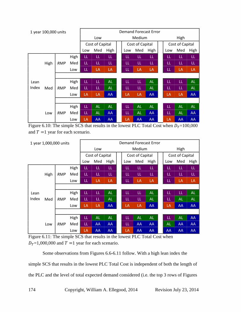
174 Copyright, William A. Ellegood, 2014 Revision July 23, 2014
1 year 100,000 units Demand Forecast Error
Low Medium High
Cost of Capital Cost of Capital Cost of Capital
Low Med High Low Med High Low Med High
Lean
High RMP
High LL LL LL
LL LL LL
LL LL LL
Med LL LL LL
LL LL LL
LL LL LL
Low LL LA LA
LL LA LA
LL LA LA
Med RMP
High LL LL AL
LL LL AL
LL LL AL
Index Med LL LL AL
LL LL AL
LL LL AL
Low LA LA AA
LA LA AA
LA LA AA
Low RMP
High LL AL AL
LL AL AL
LL AL AL
Med LL AL AA
LL AL AA
LL AL AA
Low LA AA AA
LA AA AA
LA AA AA
Figure 6.10: The simple SCS that results in the lowest PLC Total Cost when =100,000
and 1 year for each scenario.
1 year 1,000,000 units Demand Forecast Error
Low Medium High
Cost of Capital Cost of Capital Cost of Capital
Low Med High Low Med High Low Med High
Lean
High RMP
High LL LL LL
LL LL LL
LL LL LL
Med LL LL LL
LL LL LL
LL LL LL
Low LL LA LA
LL LA LA
LL LA LA
Med RMP
High LL LL AL
LL LL AL
LL LL AL
Index Med LL LL AL
LL LL AL
LL AL AL
Low LA LA AA
LA LA AA
LA AA AA
Low RMP
High LL AL AL
LL AL AL
LL AL AA
Med LL AA AA
LL AA AA
AL AA AA
Low LA AA AA
LA AA AA
AA AA AA
Figure 6.11: The simple SCS that results in the lowest PLC Total Cost when
=1,000,000 and 1 year for each scenario.
Some observations from Figures 6.6-6.11 follow. With a high lean index the
simple SCS that results in the lowest PLC Total Cost is independent of both the length of
the PLC and the level of total expected demand considered (i.e. the top 3 rows of Figures

Revision July 23, 2014 Copyright, William A. Ellegood, 2014 175
6.6-6.11 are the same). Further, when the lean index is medium and the demand forecast
error is either low or medium, the simple SCS that results in the lowest PLC Total Cost is
independent of both the length of the PLC and level of total expected demand considered.
From Figures 6.6 and 6.7 for a 5 year PLC, with a low lean index there are seven
of twenty-seven scenarios where the simple SCS that results in the lowest PLC Total Cost
differs as the total expected demand is increased from 100,000 to 1 million, and in six of
those instances the simple SCS changes to a leaner SCS. The one scenario where the
lowest cost SCS become more agile is with low lean index, high RMP, medium demand
forecast error, and high cost of capital. Also from Figures 6.6 and 6.7 for a 5 year PLC,
when the lean index is medium there are three instances where the SCS changes as the
total expected demand is increased from 100,000 to 1 million units, and in all three
instances the cost of capital and demand forecast error are high. When RMP is either
medium or low the SCS becomes more agile and when RMP is high the SCS becomes
leaner. In contrast, when the PLC was one year in length, as shown in Figures 6.10 and
6.11, all eight scenarios where the simple SCS that gives the lowest PLC Total Cost
differs when total expected demand is increased from 100,000 to 1,000,000 units moves
towards a more agile SCS. Six of the instances are with a low index and six are with high
demand forecast error.
From Figures 6.6, 6.8, and 6.10, when total expected demand is 100,000 and the
length of the PLC is decreased from five years to one year and both demand forecast
error and cost of capital are not at a high level, there are six instances where the simple
SCS differs and in all six cases the SCS moves to a leaner SCS. When both demand
forecast error and cost of capital are high and the SCS that results in the lowest Total

176 Copyright, William A. Ellegood, 2014 Revision July 23, 2014
Cost differs as the length of the PLC decreases, in the majority of instances the SCS
moves towards a more agile SCS.
When Figures 6.7, 6.9, and 6.11 are examined, in nine of the ten instances where
the simple SCS differs as the length of the PLC is shortened, the simple SCS that results
in the lowest PLC Total Cost moves towards a more agile SCS. The single instance
where this is not the case occurs with low lean index, high RMP, medium demand
forecast error, high cost of capital, and the length of the PLC is shortened from 5 years to
2 years; where the simple SCS that results in the lowest PLC Total Cost changes from a
simple agile SCS to a simple agilean SCS.
In summary, based on the parameters considered, all instances where the SCS
differs because either the total expected demand or the length of the PLC is changed
occur when either the lean index level is low or when the lean index level is medium and
demand forecast error is at a high level. Under these scenarios the following changes in
simple supply chain strategies are observed. First, when total expected demand is
100,000 units and the length of the PLC is increased, a more agile SCS may reduce the
PLC Total Cost of a product. Second, in contrast to the first observation, when total
expected demand is one million units and the length of the PLC is increased, then a
leaner SCS may reduce the PLC Total Cost of a product. Third, when the length of the
PLC is 5 years and the total expected demand is increased, then a leaner SCS may reduce
the PLC Total Cost of a product. Last, conversely to the third observation, when the
length of the PLC is one year and total expected demand is increased, then a more agile
SCS may reduce the PLC Total Cost of a product. This suggests that the simple SCS that
results in the lowest PLC Total Cost for a product where the lean index level is low or

Revision July 23, 2014 Copyright, William A. Ellegood, 2014 177
when the lean index level is medium and the high demand forecast error is dependent on
both the length of the PLC and total expected demand of the product. Note that for the
majority of scenarios considered, 396 out of 486 (81%), the simple SCS that results in the
lowest PLC Total Cost is independent of both the lengths of the PLC and the total
expected demand levels considered.
From Figure 6.6, the scenarios where the complex SCS results in a lower PLC
Total Cost than any simple SCS occurs when the PLC is 5 years, total expected demand
is 100,000 units, low RMP, high lean index, and low demand forecast error. In all three of
these scenarios, a simple SCS results in a lower PLC Total Cost than the complex SCS
when total expected demand is increased to one million units. Table 6.4 gives the percent
difference between the PLC Total Cost of the complex SCS and the simple SCS that
results in the lowest PLC Total Cost. In all three cases the NPV cost advantage of the
complex SCS is very small (<0.1%) compared to the best simple SCS. The Total Cost
difference between the best simple SCS and the complex SCS is also presented in Table
6.4, with the largest difference being just under $6,100 over 5 years.
Cost of Capital
(Annually) Low (5%) Medium (10%) High (15%)
Percent Difference 0.018% 0.080% 0.007%
Total Cost Difference $1,560 $6,073 $438
Table 6.4: Percent difference in the PLC Total Cost of the complex SCS and the best
simple SCS
To determine the approximate total expected demand that minimizes the
difference between the PLC Total Cost of the complex SCS and the simple SCS with the
lowest PLC Total Cost, the model is evaluated for total expected demand values from
100,000 to 1 million in increments of 100,000. The PLC Total Cost of the complex SCS

178 Copyright, William A. Ellegood, 2014 Revision July 23, 2014
and a simple lean SCS are approximately equal when the total expected demand is
700,000 units and the cost of capital is 5% annually (low level). When the cost of capital
is increased to a medium level (10% annually), the PLC Total Cost of a complex SCS
and a simple leagile SCS are approximately equal when the total expected demand is
400,000 units. The PLC Total Cost of the complex SCS and a simple leagile SCS are
nearly equal when the total expected demand is slightly more than 100,000 units and the
cost of capital is at a high level (15% annually).
6.3 Examples
This section presents detailed results associated with three scenarios
corresponding to: (i) a functional product, (ii) a hybrid product, and (iii) an innovative
product. The functional product has a long PLC (5 years) and the demand forecast error
and the cost of capital are at a low level. The hybrid product has a medium length PLC (2
years), medium demand forecast error, and medium cost of capital. The innovative
product has a short PLC (1 year), high demand forecast error, and high cost of capital. To
focus the discussion on the impact of product type, the RMP value for all three scenarios
examined is set at a medium level as defined in Table 6.1.
6.3.1 Functional product
Fisher (1997) described a functional product in part as a product that has a long
PLC of 2 or more years and a demand forecast error of less than 10%. This research uses
the following scenario for a functional product: (i) a PLC of 5 years and the total
expected demand for the PLC of one million units, and (ii) low demand forecast error,
low cost of capital, medium RMP, and high lean index, all as defined in Table 6.1.

Revision July 23, 2014 Copyright, William A. Ellegood, 2014 179
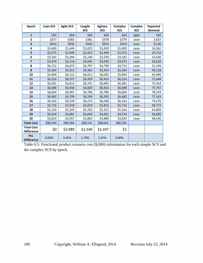
180 Copyright, William A. Ellegood, 2014 Revision July 23, 2014
Epoch Lean SCS Agile SCS Leagile SCS
Agilean SCS
Complex SCS
Complex SCS
Expected Demand
1 $65 $64 $64 $64 $64 Agile 556
2 $377 $382 $381 $378 $379 Lean 3,637
3 $914 $935 $926 $923 $914 Lean 9,130
4 $1,600 $1,644 $1,625 $1,620 $1,600 Lean 16,362
5 $2,375 $2,449 $2,415 $2,409 $2,375 Lean 24,716
6 $3,182 $3,284 $3,236 $3,230 $3,182 Lean 33,636
7 $3,974 $4,110 $4,045 $4,039 $3,974 Lean 42,626
8 $4,712 $4,875 $4,797 $4,790 $4,712 Lean 51,249
9 $5,364 $5,551 $5,461 $5,454 $5,364 Lean 59,128
10 $5,904 $6,112 $6,011 $6,005 $5,904 Lean 65,946
11 $6,314 $6,537 $6,429 $6,423 $6,314 Lean 71,444
12 $6,581 $6,814 $6,701 $6,695 $6,581 Lean 75,424
13 $6,698 $6,936 $6,820 $6,814 $6,698 Lean 77,747
14 $6,664 $6,901 $6,786 $6,780 $6,664 Lean 78,333
15 $6,482 $6,709 $6,599 $6,593 $6,482 Lean 77,163
16 $6,162 $6,378 $6,273 $6,268 $6,162 Lean 74,276
17 $5,716 $5,918 $5,819 $5,815 $5,716 Lean 69,772
18 $5,163 $5,345 $5,256 $5,252 $5,163 Lean 63,809
19 $4,524 $4,681 $4,604 $4,601 $4,524 Lean 56,605
20 $3,824 $3,957 $3,892 $3,889 $3,824 Lean 48,440
Total Cost $86,594 $89,584 $88,141 $88,041 $86,595
Total Cost Difference
$0 $2,989 $1,546 $1,447 $1
Pct. Difference
0.00% 3.45% 1.79% 1.67% 0.00%
Table 6.5: Functional product scenario cost ($,000) information for each simple SCS and
the complex SCS by epoch.

Revision July 23, 2014 Copyright, William A. Ellegood, 2014 181
Figure 6.12: Each SCS cost per epoch relative to the simple lean SCS for the functional
product scenario.
The length of each epoch of the PLC is assumed to be 9 days; therefore, a 5 year
PLC is subdivided into twenty epochs, as illustrated in Table 6.5 and Figures 6.12-6.14.
Table 6.5 shows the Total Cost of each simple SCS (columns 2-5) and the complex SCS
(column 6) per epoch, plus the relative and percentage cost difference of each SCS to the
SCS with the lowest PLC Total Cost. The complex SCS uses an agile SCS in the first
epoch and a lean SCS in all other epochs. The PLC Total Cost difference between a
simple lean SCS and the complex SCS is less than a $1,000 over five years. Table 6.5
also shows that choosing an inappropriate simple SCS can result in a considerable Total
Cost impact over the PLC. A simple agile SCS will cost approximately $3 million more
than a simple lean SCS and a simple leagile SCS or a simple agilean SCS will cost
approximately $1.5 million more than a simple lean SCS. Figure 6.12 illustrates the cost
difference of each SCS relative to the lowest PLC Total Cost SCS (simple lean SCS) for
each epoch. From Figure 6.12, early in the PLC when expected demand is low, the
relative cost difference between each simple supply chain strategy and the lowest PLC
$0
$50
$100
$150
$200
$250
$300
0 5 10 15 20
SCS
Co
st D
iffe
ren
ce
($,0
00
)
Epoch
SCS cost relative to a simple lean SCS cost
Complex
Agile
Leagile
Agilean

182 Copyright, William A. Ellegood, 2014 Revision July 23, 2014
Total Cost SCS is small. However, as the expected demand per epoch increases the cost
impact of adopting a less effective SCS becomes significant, and may exceed $230
thousand an epoch for a simple agile SCS.
Figure 6.13: Functional product scenario
per epoch for each SCS.
Figure 6.14: Functional product scenario
per epoch for each SCS.
Figure 6.13 shows the optimal number of supply side ordering periods,
, and
Figure 6.14 shows the optimal number of demand side ordering periods,
, for each
-
10
20
30
40
50
1 2 3 4 5 6 7 8 9 10 11 12 13 14 15 16 17 18 19 20
Ord
erin
g P
erio
ds
Epoch
NSq* Lean
Agile
Leagile
Agilean
Complex
-
10
20
30
40
50
1 2 3 4 5 6 7 8 9 10 11 12 13 14 15 16 17 18 19 20
Ord
erin
g P
erio
ds
Epoch
NDq* Lean
Agile
Leagile
Agilean
Complex

Revision July 23, 2014 Copyright, William A. Ellegood, 2014 183
epoch of the various supply chain strategies. In Figure 6.13 and Figure 6.14 the bars
showing the number of ordering periods for the complex SCS are shaded with the color
of the SCS for that epoch of the PLC. Note for the supply side, the number of ordering
periods for the simple lean and the simple leagile supply chain strategies and the number
of ordering periods per epoch for the simple agile and the simple agilean supply chain
strategies are the same for each epoch of the PLC, because the pairs of supply chain
strategies share the same supply side strategy. Similarly, for the demand side the number
of ordering periods for the simple lean SCS and the simple agilean SCS are equal, and the
number of ordering periods per epoch for the simple agile SCS and the simple agilean
SCS are the same for each epoch of the PLC, because the pairs of supply chain strategies
share the same demand side strategy.
From Figure 6.13, the optimal number of orders when a lean strategy is
considered for the supply side is constrained by the frequency that orders could be made
(6 orders per epoch). From Figure 6.13, on the supply side with the lean strategy there
were three orders for the first epoch and six orders for each of the remaining epochs.
From Figure 6.14, the optimal number of orders when a lean strategy is considered for
the demand side is constrained by the frequency that orders could be made (15 orders per
epoch), with three orders for the first epoch and fifteen orders for each of the remaining
epochs. The optimal number of orders for an agile strategy was limited to one order per
day or 90 orders per epoch. With the agile strategy the optimal number of orders
increased steadily on both sides of the supply chain as the expected demand increased,
then stabilized at 45 orders per epoch; as total expected demand per epoch decreased the
optimal number orders per epoch decreased.
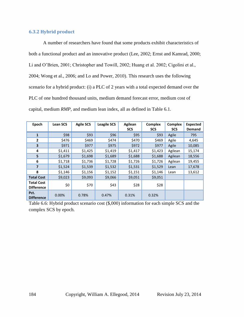
184 Copyright, William A. Ellegood, 2014 Revision July 23, 2014
6.3.2 Hybrid product
A number of researchers have found that some products exhibit characteristics of
both a functional product and an innovative product (Lee, 2002; Ernst and Kamrad, 2000;
Li and O’Brien, 2001; Christopher and Towill, 2002; Huang et al. 2002; Cigolini et al.,
2004; Wong et al., 2006; and Lo and Power, 2010). This research uses the following
scenario for a hybrid product: (i) a PLC of 2 years with a total expected demand over the
PLC of one hundred thousand units, medium demand forecast error, medium cost of
capital, medium RMP, and medium lean index, all as defined in Table 6.1.
Epoch Lean SCS Agile SCS Leagile SCS Agilean SCS
Complex SCS
Complex SCS
Expected Demand
1 $98 $93 $96 $95 $93 Agile 795
2 $476 $469 $474 $470 $469 Agile 4,645
3 $971 $977 $975 $972 $977 Agile 10,085
4 $1,411 $1,425 $1,419 $1,417 $1,423 Agilean 15,174
5 $1,679 $1,698 $1,689 $1,688 $1,688 Agilean 18,556
6 $1,718 $1,736 $1,728 $1,726 $1,726 Agilean 19,455
7 $1,524 $1,539 $1,532 $1,531 $1,529 Lean 17,678
8 $1,146 $1,156 $1,152 $1,151 $1,146 Lean 13,612
Total Cost $9,023 $9,093 $9,066 $9,051 $9,051
Total Cost Difference
$0 $70 $43 $28 $28
Pct. Difference
0.00% 0.78% 0.47% 0.31% 0.32%
Table 6.6: Hybrid product scenario cost ($,000) information for each simple SCS and the
complex SCS by epoch.

Revision July 23, 2014 Copyright, William A. Ellegood, 2014 185
Figure 6.15: Supply chain strategies of the complex SCS for the hybrid product scenario.
Figure 6.16: Each SCS cost per epoch relative to the simple lean SCS for the hybrid
product scenario.
Table 6.6 shows that a simple lean SCS results in a slightly lower PLC Total Cost
than a simple agilean SCS or a complex SCS. The complex SCS is a combination of three
supply chain strategies, an agile SCS for the first three epochs, then an agilean SCS for
0
50
100
150
200
250
0 1 2 3 4 5 6 7 8
dj
Epoch
Hybrid Product Complex SCS
AgileAgileanLean
T
-$10
-$5
$0
$5
$10
$15
$20
1 2 3 4 5 6 7 8
SCS
Co
st D
iffe
ren
ce
($,0
00
)
Epoch
Complex
Agile
Leagile
Agilean

186 Copyright, William A. Ellegood, 2014 Revision July 23, 2014
the next three epochs and a lean SCS for the last two epochs, shown in Figure 6.15. The
combination of supply chain strategies shown in Table 6.6 and Figure 6.15 is similar to
the scheme presented in Figure 1.3, where an agile SCS is employed in the introduction
stage of the PLC, changes to a compound SCS (leagile or agilean SCS), and finally ends
the PLC with a lean SCS. As seen in Figures 6.6-6.11, the compound simple supply chain
strategies (leagile SCS and agilean SCS) are more likely to result in the lowest PLC Total
Cost when RMP is either high (simple agilean SCS) or low (simple leagile SCS).
If the supply chain elects to continue to use the SCS that results the lowest Total
Cost for the first epoch, a simple agile SCS, then the NPV cost to the supply chain would
be approximately $70,000 (0.8%) more than the minimal cost SCS over the PLC, and the
agile SCS is the least effective SCS for minimizing the Total Cost over the PLC for this
scenario. Figure 6.16 and Table 6.6 show that the NPV cost of a complex SCS is lower
than that of the simple lean SCS for the first two epochs, but from the third to the seventh
epoch the simple lean SCS provided a lower NPV cost per epoch than the complex SCS.
The NPV cost of the simple lean SCS and the complex SCS are equal for the eighth
epoch of the PLC.

Revision July 23, 2014 Copyright, William A. Ellegood, 2014 187
Figure 6.17: Hybrid product scenario
per epoch for each SCS
Figure 6.18: Hybrid product scenario
per epoch for each SCS.
Figure 6.17 shows the optimal number of supply side ordering periods,
, and
Figure 6.18 shows the optimal number of demand side ordering periods,
, for each
epoch of the various supply chain strategies for the hybrid product scenario. In Figure
6.17 and Figure 6.18 the bars showing the number of ordering periods for the complex
0
5
10
15
20
1 2 3 4 5 6 7 8
Ord
erin
g P
erio
ds
Epoch
NS*
Lean
Agile
Leagile
Agilean
Complex
-
5
10
15
20
1 2 3 4 5 6 7 8
Ord
erin
g P
erio
ds
Epoch
ND*
Lean
Agile
Leagile
Agilean
Complex

188 Copyright, William A. Ellegood, 2014 Revision July 23, 2014
SCS are shaded with the color of the SCS of the complex SCS for that epoch of the PLC.
From Figure 6.17, the optimal number of orders when a lean strategy is used for the
supply side is always six, which reflects the constraint on the frequency that orders can be
made. On the demand supply side, Figure 6.18, with the lean strategy there are fifteen
orders in every epoch, except the last epoch, which uses nine orders. The optimal number
of orders for an agile strategy is limited to one per day or 90 orders per epoch. With the
agile strategy the optimal number of orders increases quickly to 18 orders per epoch
starting with the second epoch for both sides of the supply chain, and as total expected
demand per epoch decreases the optimal number orders per epoch decreases.
6.3.3 Innovative product
Fisher (1997) described an innovative product in part as a product that has a PLC
of 1 year or less and a demand forecast error greater than 40%. This research uses the
following scenario for an innovative product: (i) a PLC of one year with a total expected
demand for the PLC of one hundred thousand units, and (ii) high demand forecast error,
high cost of capital, medium RMP, and low lean index, all as defined in Table 6.1.
Epoch Lean SCS Agile SCS Leagile SCS Agilean SCS
Complex SCS
Complex SCS
Expected Demand
1 $653 $586 $630 $608 $586 Agile 5,440
2 $2,527 $2,452 $2,505 $2,473 $2,452 Agile 25,259
3 $3,501 $3,508 $3,507 $3,501 $3,508 Agile 38,011
4 $2,731 $2,775 $2,748 $2,758 $2,775 Agile 31,290
Total Cost $9,412 $9,320 $9,391 $9,341 $9,320
Total Cost Difference
$92 $0 $71 $20 $0
Pct. Difference
0.98% 0.00% 0.76% 0.22% 0.00%
Table 6.7: Innovative product scenario cost ($,000) information for each simple SCS and
the complex SCS by epoch.

Revision July 23, 2014 Copyright, William A. Ellegood, 2014 189
Figure 6.19: Each SCS cost per epoch relative to the simple agile SCS for the innovative
product scenario.
Table 6.7 shows that the simple agile SCS and the complex SCS are the same, and
thus result in the same PLC Total Cost. For this scenario the flexibility of the complex
SCS to change strategies is not exploited: the lowest cost strategy is to use an agile SCS
in every epoch. Table 6.7 and Figure 6.19 show that for the third epoch of the PLC the
Total Costs for all the supply chain strategies considered are approximately equal and the
simple lean SCS results in the lowest Total Cost of the fourth epoch. Table 6.7 shows that
the worst of the supply chain strategies considered when the objective is NPV cost
minimization for an innovative product is a simple lean SCS, which is nearly 1% more
expensive than the simple agile SCS.
-60
-40
-20
0
20
40
60
80
100
1 2 3 4
SCS
Co
st D
iffe
ren
ce
($,0
00
)
Epoch
Complex
Lean
Leagile
Agilean

190 Copyright, William A. Ellegood, 2014 Revision July 23, 2014
Figure 6.20: Innovative product scenario
per epoch for each SCS
Figure 6.21: Innovative product scenario
per epoch for each SCS.
Figure 6.20 shows the number of supply side ordering periods,
, and Figure
6.21 shows the number of demand side ordering periods,
, for each epoch of the
various supply chain strategies for the innovative product scenario. In Figure 6.20 and
Figure 6.21 the columns showing the number of ordering periods for the complex SCS
0
10
20
30
40
50
1 2 3 4
Ord
erin
g P
erio
ds
Epoch
NSq*
Lean
Agile
Leagile
Agilean
Complex
0
10
20
30
40
50
1 2 3 4
Ord
eri
ng
Per
iod
s
Epoch
NDq*
Lean
Agile
Leagile
Agilean
Complex

Revision July 23, 2014 Copyright, William A. Ellegood, 2014 191
are shaded with the color of the SCS of the complex SCS for that epoch of the PLC.
From Figure 6.20 and 6.21, the optimal number of orders when a lean strategy is used for
both the supply side and the demand side appears to be constrained by the frequency at
which orders can be made. For both the supply side and the demand side when a lean
strategy is considered, the maximum allowable number of orders per epoch is employed
for all epochs. The optimal number of orders for an agile strategy is limited to 90 orders
per epoch. With the agile strategy the optimal number of orders per epoch started at 45
orders for both sides of the supply chain and only decreases during the fourth epoch as
total expected demand per epoch decreases.
Considering the three scenarios presented in this section the following statements
can be made. (i) For the functional and innovative product, adopting the complex SCS
results in a PLC Total Cost that is almost as low as or the same as the best simple SCS.
(ii) The worst product type to adopt a complex SCS for is the hybrid product. (iii)
Adopting the wrong strategy can have a significant cost impact, and this impact is the
greatest when a wrong strategy is adopted for a functional product.
6.4 Agile SCS to a lean SCS
In Figure 1.3, a scenario is presented where the SCS of a product evolves over the
life-cycle: starting with an agile SCS, then evolving to a compound SCS (leagile or
agilean), and then evolving again to a lean SCS. Although the research findings
demonstrates for the majority of scenarios considered that a supply chain should adopt a
single SCS to minimize PLC Total Cost, this section examines the question of how the
SCS should evolve for those supply chains that plan to evolve the SCS as the product
progresses through its PLC. As the supply chain goes from an agile SCS to a compound

192 Copyright, William A. Ellegood, 2014 Revision July 23, 2014
SCS, which side (demand or supply) of the supply chain should evolve first? Evolving
the supply side first means the supply chain will evolve to a leagile SCS, and evolving
the demand side first means the supply chain will evolve to an agilean SCS. From this
research it is observed that when evolving the SCS over the PLC the lowest cost SCS is
more sensitive to the RMP of the supply chain. Three scenarios are considered with RMP
at a different level for each scenario and the other characteristics of the scenarios are
constant: medium lean index, low cost of capital, and medium demand forecast error. The
length of the PLC for each scenario was 2 years and was one million units. The three
scenarios are of a hybrid product type; however, this analysis is independent of the
product type and would apply to a functional product employing an agile SCS and is
evolving the SCS to a lean SCS.
6.4.1 High RMP
The first scenario considered is with high RMP. The costs per epoch for each
simple SCS and the complex SCS, as well as the strategy of the complex SCS per epoch
are presented in Table 6.8.

Revision July 23, 2014 Copyright, William A. Ellegood, 2014 193
Epoch Lean SCS Agile SCS Leagile SCS Agilean SCS
Complex SCS
Complex SCS
Expected Demand
1 $918 $860 $868 $911 $860 Agile 7,947 2 $4,723 $4,707 $4,715 $4,716 $4,707 Agile 46,453 3 $9,858 $10,004 $9,993 $9,869 $10,004 Agilean 100,846 4 $14,548 $14,832 $14,807 $14,574 $14,768 Agilean 151,739 5 $17,545 $17,904 $17,871 $17,578 $17,574 Lean 185,559 6 $18,171 $18,541 $18,507 $18,205 $18,171 Lean 194,553 7 $16,318 $16,640 $16,613 $16,346 $16,318 Lean 176,781 8 $12,420 $12,653 $12,633 $12,440 $12,420 Lean 136,121
Total Cost $94,503 $96,142 $96,008 $94,638 $94,824
Total Cost Difference
$0 $1,638 $1,505 $134 $321
Pct. Difference
0.00% 1.45% 0.74% 0.71% 0.30%
Table 6.8: High RMP scenario cost ($,000) information for each simple SCS and the
complex SCS by epoch.
Figure 6.22: Each SCS cost per epoch relative to the simple lean SCS for a scenario with
high RMP.
For the scenario presented in Table 6.8 and Figure 6.22, if a supply chain wants to
evolve the SCS from an agile SCS to a lean SCS, to minimize the cost impact to the
supply chain, the demand side of the supply chain should evolve first to an agilean SCS.
Then, later, the supply side should evolve to complete the evolution to a lean SCS. In this
-$100
$0
$100
$200
$300
$400
1 2 3 4 5 6 7 8SCS
Co
st D
iffe
ren
ce
Tho
usa
nd
s
Epochs
SCS cost relative to a simple lean SCS cost
Complex
Agile
Leagile
Agilean
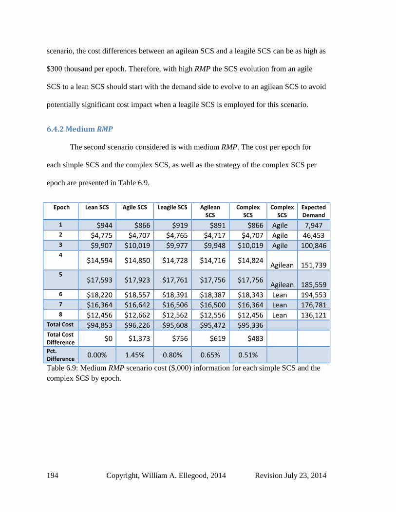
194 Copyright, William A. Ellegood, 2014 Revision July 23, 2014
scenario, the cost differences between an agilean SCS and a leagile SCS can be as high as
$300 thousand per epoch. Therefore, with high RMP the SCS evolution from an agile
SCS to a lean SCS should start with the demand side to evolve to an agilean SCS to avoid
potentially significant cost impact when a leagile SCS is employed for this scenario.
6.4.2 Medium RMP
The second scenario considered is with medium RMP. The cost per epoch for
each simple SCS and the complex SCS, as well as the strategy of the complex SCS per
epoch are presented in Table 6.9.
Epoch Lean SCS Agile SCS Leagile SCS Agilean SCS
Complex SCS
Complex SCS
Expected Demand
1 $944 $866 $919 $891 $866 Agile 7,947 2 $4,775 $4,707 $4,765 $4,717 $4,707 Agile 46,453 3 $9,907 $10,019 $9,977 $9,948 $10,019 Agile 100,846 4
$14,594 $14,850 $14,728 $14,716 $14,824 Agilean 151,739
5 $17,593 $17,923 $17,761 $17,756 $17,756
Agilean 185,559
6 $18,220 $18,557 $18,391 $18,387 $18,343 Lean 194,553 7 $16,364 $16,642 $16,506 $16,500 $16,364 Lean 176,781 8 $12,456 $12,662 $12,562 $12,556 $12,456 Lean 136,121
Total Cost $94,853 $96,226 $95,608 $95,472 $95,336
Total Cost Difference
$0 $1,373 $756 $619 $483
Pct. Difference
0.00% 1.45% 0.80% 0.65% 0.51%
Table 6.9: Medium RMP scenario cost ($,000) information for each simple SCS and the
complex SCS by epoch.

Revision July 23, 2014 Copyright, William A. Ellegood, 2014 195
Figure 6.23: Each SCS cost per epoch relative to the simple lean SCS for a scenario with
medium RMP.
For the scenario presented in Table 6.9 and Figure 6.23 with medium RMP, if a
supply chain wants to evolve the SCS from an agile SCS to a lean SCS, the relative cost
difference of first switching the demand side versus the supply side is very small. From
Table 6.9, starting with epoch 4, the first epoch the complex SCS evolves, the cost
differences between an agilean SCS and a leagile SCS are at most $12,000 per epoch.
Therefore, to evolve the supply chain from an agile SCS to a lean SCS with a medium
RMP for the scenario considered, the supply chain should most likely base their selection
of the side of the supply chain to start with on factors other than cost.
6.4.3 Low RMP
The third scenario considered is with low RMP. The cost per epoch for each
simple SCS and the complex SCS, as well as the strategy of the complex SCS per epoch
are presented in Table 6.10.
-$100
$0
$100
$200
$300
$400
1 2 3 4 5 6 7 8SCS
Co
st D
iffe
ren
ce
Tho
usa
nd
s
Epochs
SCS cost relative to a simple lean SCS cost
Complex
Agile
Leagile
Agilean

196 Copyright, William A. Ellegood, 2014 Revision July 23, 2014
Epoch Lean SCS Agile SCS Leagile SCS Agilean SCS
Complex SCS
Complex SCS
Expected Demand
1 $969 $861 $964 $866 $861 Agile 7,947 2 $4,826 $4,711 $4,817 $4,720 $4,711 Agile 46,453 3 $9,955 $10,012 $9,950 $10,017 $10,012 Agile 100,846 4 $14,640 $14,844 $14,637 $14,847 $14,844 Agile 151,739 5 $17,640 $17,918 $17,638 $17,921 $17,918 Agile 185,559 6 $18,269 $18,555 $18,266 $18,559 $18,487 Leagile 194,553 7 $16,410 $16,653 $16,404 $16,660 $16,404 Leagile 176,781 8 $12,492 $12,663 $12,487 $12,669 $12,487 Leagile 136,121
Total Cost $95,202 $96,216 $95,162 $96,259 $95,723
Total Cost Difference
$40 $1,054 $0 $1,097 $561
Pct. Difference
0.04% 1.11% 0.00% 1.15% 0.59%
Table 6.10: Low RMP scenario cost ($,000) information for each simple SCS and the
complex SCS by epoch.
Figure 6.24: Each SCS cost per epoch relative to the simple lean SCS for a scenario with
low RMP.
For the scenario presented in Table 6.10 and Figure 6.24, if a supply chain wanted
to evolve the SCS from an agile SCS to a lean SCS, to minimize the cost impact the
supply chain should change the supply side first and evolve to a leagile SCS, and then
later, evolve the demand side to complete the evolution to a lean SCS. In this scenario,
-$200
-$100
$0
$100
$200
$300
$400
1 2 3 4 5 6 7 8
SCS
Co
st D
iffe
ren
ce
Tho
usa
nd
s
Epoch
SCS cost relative to a simple lean SCS cost
Complex
Agile
Leagile
Agilean
Revision July 23, 2014 Copyright, William A. Ellegood, 2014 197
the cost differences between a leagile SCS and an agilean SCS can be as high as $290
thousand per epoch. Therefore, with low RMP the SCS evolution from an agile SCS to a
lean SCS should start with the supply side to avoid potentially significant cost impact of
using an agilean SCS.
6.5 Summary
The analysis found that for 483 of the 486 (99.4%) scenarios examined (shown in
Figures 6.6-6.11) a simple SCS resulted in the same or lower PLC Total Cost than a
complex SCS, when PLC Total Cost is determined using a rolling horizon heuristic. The
research presented in this chapter supported analytically the research of Randall and
Ulrich (2001), Cigolini (2004), Stradtler (2005), Juttner et al. (2006), Vonderembse et al.
(2006), and Seuring (2009) that in most cases the SCS of a product should be determined
prior to the product’s introduction to the market and the SCS should be fixed for the
entire PLC. There were only a very few situations identified when the minimum cost
solution was to change the SCS during the PLC.
The analysis found for the values considered that when the lean index was high or
when the lean index was medium and demand forecast error was either low or medium
the simple SCS that resulted in the lowest PLC Total Cost was independent of the length
of the PLC and the total expected demand. In addition, the research found for those
scenarios where the simple SCS that resulted in the lowest PLC Total Cost was
dependent on the length of the PLC, when the PLC length was long, as for a functional
product, and total expected demand was increased, then the simple SCS that resulted in
the lowest PLC Total Cost moved towards a leaner SCS. In contrast, when the PLC
length was short (as for an innovative product) and total expected demand was increased,
198 Copyright, William A. Ellegood, 2014 Revision July 23, 2014
then the simple SCS that resulted in the lowest PLC Total Cost moved towards a more
agile SCS.
The results of the scenario analysis presented in section 6.2 and the examples
examined in 6.3 supported the validity of the model presented in this research. For
products that were easily classified as functional or innovative (as under the Fisher
Model) and when total production costs were split evenly between the supply side and the
demand side, then the appropriate simple SCS to minimize PLC Total Cost was a simple
lean SCS for a functional product and a simple agile SCS for an innovative product.
However, one significant insight provided by this research arises from products that were
not easily classified as functional or innovative or when total production costs were not
split evenly between the supply side and demand side. This research found that when the
majority of total production costs were incurred at the manufacturer, then a simple
agilean SCS may result in the lowest PLC Total Cost; and when the majority of total
production costs were incurred at the supplier, then a simple leagile SCS may result in the
lowest PLC Total Cost.
The analysis presented in section 6.4 demonstrated the financial impact of the
decision of which side of the supply chain to evolve first when going from an agile SCS
to a lean SCS. The analysis demonstrated that when a supply chain evolved from an agile
SCS to a leaner SCS, the supply chain should start with the side of the supply chain
where the majority of the costs are incurred.
Revision July 23, 2014 Copyright, William A. Ellegood, 2014 199
7. Conclusion
The purpose of this research was to address three fundamental questions related to
supply chain strategy selection. The first question (addressed in Chapter 4) focused on the
Fisher Model: Under what circumstances does a supply chain with a “Mismatch” of SCS
and product type outperform a supply chain with a “Match” of SCS and product type.
Specifically, the questions addressed were: “When would an agile SCS minimize the total
cost of a supply chain when the product had demand characteristics of a functional
product, and when would a lean SCS minimize the total cost of the supply chain when the
product had demand characteristics of an innovative product?”
The second question (addressed in Chapter 5) is: When does each SCS minimize
the total supply chain cost for a forecast period? To address this question the research
first considered the setting where expected demand was constant for the forecast period,
and then extended this setting to the impact on the best SCS when expected demand was
allowed to increase or decrease linearly over the forecast period.
The third question considered by this research (addressed in Chapter 6) was:
Which SCS minimized total supply chain cost over the classical life-cycle of a product?
Six different production circumstances were examined.
This research presented an original analytical model of a three echelon supply
chain with two inventory points to determine the total cost of each SCS for a forecast
period when expected demand and demand forecast error were functions of time (Chapter
3). The first question was examined considering two supply chain strategies (lean SCS
and agile SCS), with expected demand and demand forecast error assumed constant for

200 Copyright, William A. Ellegood, 2014 Revision July 23, 2014
the forecast period. The second question was examined considering four supply chain
strategies (lean SCS, leagile SCS, agile SCS, and agilean SCS), with demand forecast
error assumed constant and expected demand a linear function of time over the forecast
period. The third question was examined considering four simple supply chain strategies
(lean SCS, leagile SCS, agile SCS, and agilean SCS) and a complex SCS that combined
the simple strategies, with demand forecast error modeled as an exponential decay
function with respect to time, and expected demand modeled to mimic the Classical PLC.
7.1 Findings
This research presented an original analytical model to determine the total NPV
supply chain cost for a supply chain setting that included three echelons and two
inventory points. The convexity of the model was evaluated with the hypothesis H1.
To address the first fundamental research question, “Under what circumstances
does a supply chain with a misaligned SCS and product type outperform a supply chain
with an aligned SCS and product type?” six hypotheses were presented, two to
specifically evaluate the question and four to examine the propensity of a supply chain to
move towards either a lean SCS or an agile SCS as an aspect of the supply chain was
changed.

Revision July 23, 2014 Copyright, William A. Ellegood, 2014 201
# Hypothesis Description Accepted Rejected
H1 When demand is constant there are values for the number
of ordering periods, and
, which minimizes
( ) for the forecast period [ ]. X
H2
The total cost of an agile SCS can be less than that of a
lean SCS when demand forecast error is low, and an agile
SCS becomes more attractive as the ratio of
manufacturing cost to purchased material cost decreases,
lean index decreases, and cost of capital increases.
X
H3
The total cost of a lean SCS can be less than that of an
agile SCS when demand forecast error is high, and a lean
SCS becomes more attractive as the ratio of
manufacturing cost to purchased material cost increases,
lean index increases, and cost of capital decrease.
X
H4 As the ratio of total production cost to total order
processing cost increases, the supply chain’s propensity
towards a lean SCS increases.
X
H5 As the expected daily demand rate increases, the supply
chain’s propensity towards a lean SCS increases. X
H6 When the ratio
increases, the supply chain’s
propensity towards an agile SCS increases. X
H7 When the service level of the agile SCS increases, the
supply chain’s propensity towards a lean SCS increases. X
Table 7.1: Summary of hypotheses testing.
To address the second fundamental research question, “Under what combination
of supply chain characteristics does each SCS minimize total supply chain cost?”, the
analysis was completed in two stages. For the first stage the demand forecast error and
expected demand were assumed constant over the forecast period, and each of the eighty-
one scenarios were evaluated to determine which of the four SCS resulted in the lowest
total cost. The analysis showed that a compound SCS (leagile SCS or agilean SCS) was
likely to result in the lowest total cost when RMP was either low or high. A leagile SCS
should be considered when the majority of production costs were located at the supplier
and an agilean SCS should be considered when the majority of production costs occur at
the manufacturer.

202 Copyright, William A. Ellegood, 2014 Revision July 23, 2014
The second stage was accomplished by employing a sensitivity analysis of the
findings of the first step with respect to the two aspects of the supply chain that would
generally be the most uncertain: expected demand and demand forecast error. The eighty-
one scenarios were evaluated at seven levels of expected demand percent change over the
forecast period. The SCS that resulted in the lowest SCS was insensitive to a reasonable
change in the expected daily demand rate for every scenario except one.
The final part of the sensitivity analysis in stage two examined those scenarios
where the SCS that resulted in the lowest total cost was dependent on the level of demand
forecast error. In all scenarios examined, as demand forecast error increased the SCS
moved towards a more agile SCS.
To address the third fundamental research question, “Which SCS minimized total
supply chain cost over the classical life-cycle of a product? “, the analysis considered six
product situations. Each product situation was evaluated for the eighty-one scenarios and
the PLC total cost was determined using a rolling horizon heuristic. The analysis found
that for almost all combinations of scenario and situation that a single SCS over the PLC
(simple SCS) would result in the same or lower PLC total cost than a SCS strategy where
more than one SCS could be adopted over the PLC (complex SCS). These findings
analytically support prior research, that in most cases the SCS of a product should be
determined prior to the product’s introduction to the market and the SCS should be fixed
for the entire PLC.
The research found that the for a large majority of the scenarios, the SCS that
resulted in the lowest total cost was independent of both the lengths of the PLC and the
total expected demand levels considered. When the simple SCS that resulted in the lowest

Revision July 23, 2014 Copyright, William A. Ellegood, 2014 203
PLC total cost was dependent on the length of the PLC or the total expected demand,
then the research found: (i) when the PLC length was that of a functional product and
total expected demand was increased, then the simple SCS that resulted in the lowest
PLC total cost moved towards a leaner SCS, (ii) when the PLC length was that of an
innovative product and total expected demand was increased, then the simple SCS that
resulted in the lowest PLC total cost moved towards a more agile SCS, (iii) when total
expected demand was low and the length of the PLC was increased, a more agile SCS
may reduce the PLC total cost of a product, and (iv) when total expected demand was
high and the length of the PLC was increased a leaner SCS may reduce the PLC total cost
of a product.
The scenario analysis in Chapter 6 demonstrated support for the Fisher Model, in
that for those products which can clearly be classified as either functional or innovative,
the appropriate simple SCS to minimize PLC total cost was a simple lean SCS and a
simple agile SCS, respectively. However, the significant advantage of the model
presented in this research was its applicability to scenarios where the product was not
easily classified as either functional or innovative. In addition, the versatility of the model
allows a supply chain to examine a wide range of scenarios and to evaluate the sensitivity
of the total cost to various parameters.
7.2 Managerial insights
The following are key managerial insights from this research, which are limited to
the range of parameters and scenarios examined in the dissertation and may not be
applicable to settings outside of these conditions.
204 Copyright, William A. Ellegood, 2014 Revision July 23, 2014
1. For functional products with stable demand and a low lean index, when the
majority of production costs are incurred early in the supply chain or when risk
associated with carrying inventory is high, then an agile SCS may result in a
lower total cost than a lean SCS.
2. For innovative products with unstable demand and a medium lean index, when
the majority of production costs are incurred late in the supply chain or when risk
associated with carrying inventory is low, then a lean SCS may result in a lower
total cost than an agile SCS.
3. For supply chains where the majority of costs are incurred late in the supply
chain, an agilean SCS may minimize total cost.
4. For supply chains where the majority of costs are incurred early in the supply
chain a leagile SCS may minimize total cost.
5. For most supply chains, the expected daily demand rate can be assumed constant
when determining the SCS that minimizes total cost.
6. With a high lean index or a medium lean index and a low to medium demand
forecast error, the SCS that minimized the total cost is independent of the length
of the PLC and total expected demand.
7. For supply chains where the SCS that results in the lowest cost is dependent upon
the length of the PLC and/or the total expected demand: (i) for products with
supply chains where the total expected demand is high and the length of PLC
increases, or where the length of the PLC is long and total expected demand
increases a leaner SCS may improve total cost, and (ii) for products with supply
chains where the PLC lengthens and total expected demand is low or total

Revision July 23, 2014 Copyright, William A. Ellegood, 2014 205
expected demand increase and the PLC is short, a more agile SCS may improve
total cost.
8. For supply chains that plan to evolve the SCS from an agile SCS to a lean SCS,
the supply chain should evolve the side where the majority of production costs are
incurred and when production costs are similar for the supply side and demand
side, then the supply chain should consider other factors than only cost to
determine the side to evolve first.
7.3 Contributions
This research provides a number of contributions to the literature concerning
supply chain strategy selection. First, the research developed an original analytical model
that accounted for the time value of money in a supply chain setting with three echelons
and two inventory points to determine the total NPV supply chain cost. Second, the
research describes the supply chain characteristics where a “Mismatch” between SCS and
product type may be desirable to minimize costs. Third, the research provides insight into
how where costs are incurred in the supply chain (supply side vs. demand side) impacts
the selection of the appropriate SCS. Fourth, the research demonstrated when the
expected daily demand rate is relatively high, the best SCS to minimize total cost is
insensitive to reasonable levels of change in the expected daily demand rate. Fifth, the
research provides managerial insights to the impact the length of a PLC and the level of
total expected demand has on the appropriate SCS to minimize total cost. Finally, the
research presents a new SCS concept, agilean SCS, not yet discussed in the literature,
and demonstrates when an agilean SCS may be the appropriate SCS to minimize total
cost.

206 Copyright, William A. Ellegood, 2014 Revision July 23, 2014
7.4 Limitations
There were a number of limitations associated with the research.
1. The model examined a wide range of parameters, but acknowledged that not all
possible scenarios were considered and the findings may not be applicable for
scenarios outside the range of parameters considered.
2. There may exist locally optimal results within the range of parameters considered
that were not discovered.
3. The model was developed as a planning model to analyze expected demand and
did not respond dynamically to changes in actual demand.
4. The model was developed and was only effective for supply chains that employ a
periodic review inventory replenishment system.
5. The lead time of the supply chain strategies were assumed constant.
6. The model assumed realized demand was normally distributed about expected
demand and for some products there could be other distributions that may be
more appropriate.
7. The function used to describe the classical PLC was developed for this research
and did not necessarily describe the expected demand of all products that had a
classical PLC.
8. The classical PLC presented in this research was just one of several product life-
cycles that had been discussed in literature and did not necessarily describe the
life-cycle of all products.

Revision July 23, 2014 Copyright, William A. Ellegood, 2014 207
7.5 Opportunities for future research
Both the area of the supply chain strategy selection and the analytical model
developed in this research offer a variety of future research opportunities. For example, a
survey methodology could be employed to determine the impact the supply chain and
product characteristics presented in this research (RMP, lean index, demand forecast error
and cost of capital), along with other characteristics, have on practitioners’ choices when
selecting a SCS for a product. Another opportunity for future research could involve
further analysis of parameters affecting the model, but not considered fully in this
research (e.g., value of ). Although the findings of this research support the validity
of the model presented within, a third opportunity for future research is validating the
model with real industry supply chain data. A fourth opportunity for future research is
determining the optimal complex SCS and optimal simple SCS with mathematical
programming that considers relaxed replenishment policy constraints, with the results
evaluated against the findings of this research. Another opportunity for future research is
considering different definitions of a leagile SCS; for example the model can be
restructured to consider the “base and surge” and the Pareto definitions of leagile SCS to
provide further insight to the appropriate SCS to minimize total cost. Lastly, the
discussion concerning the agilean SCS can be expanded. One possible example of the
agilean SCS is Toyota Motors Corporation, where on the demand side of the supply chain
95% of Toyota vehicles are produced to forecasted demand, while the supply side of the
supply chain is very agile with many suppliers making multiple deliveries to Toyota
assembly facilities daily.

208 Copyright, William A. Ellegood, 2014 Revision July 23, 2014
Works cited
Agarwal, A., Shankar, R., & Tiwari, M. (2006). Modeling the metrics of lean, agile and
leagile supply chian: An ANP-based approach. European Journal of Operational
Research, 173, 211-225.
Ahn, H., & Kaminsky, P. (2005). Production and distribution policy in a two-stage
stochastic push-pull supply chain. IIE Transactions, 37, 609-621.
Aitken, J., Childerhouse, P., & Towill, D. (2003). The impact of product life cycle on
supply chain strategy. International Journal of Production Economics, 85, 127-
140.
Aitken, J., Christopher, M., & Towill, D. (2002). Understanding, implementing and
exploiting agilityand leanness. International Journal of Logistics: Research and
Applications, 5(1), 59-74.
Argelo, S. (1992). Integral Logistics Structures: Developing Customer Oriented Goods
Flow. (S. Hoekstra, & J. Romme, Eds.) New York, NY: McGraw-Hill.
Aviv, Y. (2001). The effect of collaborative forecasting on supply chain performance.
Management Science, 47(10), 1326-1343.
Besbes, K., Allaoui, H., Goncalves, G., & Loukil, T. (2012). A two-phase approach for
supply chain design with product life cycle and green procurement considerations.
Proceedings of MOSIM'12. Bordeaux.
Catalan, M., & Kotzab, H. (2003). Assessing the responsiveness in the Danish mobile
phone supply chain. International Journal of Physical Distribution & Logistics,
33(8), 668-85.
Cheung, K. L., & Lee, H. L. (2002). The inventory benefit of shipment coordination and
stock rebalancing in a supply chain. Management Science, 48(2), 300-306.
Chiang, W.-y. K., Chhajed, D., & Hess, J. D. (2003). Direct marketing, indirect profits: A
strategic analysis of dual-channel supply-chain design. Management Science,
49(1), 1-20.
Childerhouse, P., Aitken, J., & Towill, D. (2002). Analysis and design of focused demand
chains. Journal of Operations Management, 20, 675-689.
Christopher, M. (1992). Logistics & Supply Chain Management. London: Pitmans.
Christopher, M., & Towill, D. (2000). Marrying lean and agile paradigms. Proceedings of
EUROMA, (pp. 114-121). Ghent, Belgium.

Revision July 23, 2014 Copyright, William A. Ellegood, 2014 209
Christopher, M., & Towill, D. (2001). An integrated model for the design of agile supply
chain. International Journal of Physical Distribution & Logistics Management,
31(4), 235-46.
Christopher, M., & Towill, D. (2002). Developing market specific supply chain
strategies. International Journal of Logistics Management, 13(1), 1-14.
Christopher, M., Peck, H., & Towill, D. (2006). A taxonomy for selectign global supply
chain strategies. The International Journal of Logistics Management, 17(2), 277-
287.
Cigolini, R., Cozzi, M., & Perona, M. (2004). A new framework for supply chain
management. International Journal of Operations & Production Management,
24(1), 7-41.
Cox, W. J. (1967). Product life cycles as marketing models. The Journal of Business,
40(4), 375-384.
CSCMP. (n.d.). Council of Supply Chain Management Professionals Supply Chain
Management. Retrieved from http://cscmp.org/about-us/supply-chain-
management-definitions
de Treville, S., Shapiro, R., & Hameri, A. (2004). From supply chain to demand chain:
the role of lead time reduction in improving demand chain performance. Journal
of Operations Management, 21, 613-627.
Dean, J. (1950). Pricing policies for new products. Havard Business Review, 28(6), 45-
53.
Delen, D., Hardgrave, B. C., & Sharda, R. (2007). RFID for better supply-chain
management through enhanced information visibility. Production and Operations
Management, 16(5), 613-624.
Disney, S. M., & Towill, D. R. (2003). On the bullwhip and inventory variance produced
by an ordering policy. Omega: The International Journal of Management Science,
31, 157-167.
Disney, S. M., & Towill, D. R. (2003). Vendor-managed inventory and bullwhip
reduction in a two-level supply chain. International Journal of Operations&
Production Management, 23(6), 625-651.
Disney, S., & Naim, M. P. (2004). Assessing the impact of e-business on supply chain
dynamics. International Journal of Production Economics, 89, 109-118.

210 Copyright, William A. Ellegood, 2014 Revision July 23, 2014
Disney, S., Warburton, R., & Zhong, Q. (2013). Net present value analysis of the
economic production quantity. IMA Journal of Management Mathematics, 24(4),
423-435.
Ernst, R., & Kamrad, B. (2000). Evaluation of supply chain structures through
modularization and postponement. European Journal of Operational Research,
124, 495-510.
Fisher, M. (1997). What is the right supply chain for your product. Harvard Business
Review, 75(2), 105-16.
Franca, R., Jones, E., Richards, C., & Carlson, J. (2010). Multi-objective stochastic
supply chain modeling to evaluate tradeoffs between profit and quality.
International Journal of Production Economics, 127, 292-299.
Gavirneni, S., Kapuscinski, R., & Tayur, S. (1999). Value of information in capacitated
supply chains. Management Science, 45(1), 16-24.
Goldsby, T., Griffis, S., & Roath, A. (2006). Modeling lean, agile, and leagile supply
chain strategies. Journal of Business Logistics, 27(1), 57-80.
Grubbstrom, R. (1980). A principle for determining the correct capital costs of work-in-
progress and inventory. International Journal of Production Research, 18(2),
259-271.
Guillen, G., Mele, F., Bagajewicz, M., Espuna, A., & Puigjaner, L. (2005).
Multiobjective supply chain design under uncertainty. Chemical Engineering
Science, 60, 1535-1553.
Gupta, D., & Benjaafar, S. (2004). Make-to-order, make-to-stock, or delay product
differentiation? A common framework for modeling and analysis. IIE
Transactions, 36, 529-546.
Harris, G., Componation, P., & Farrington, P. (2010). An exploration of Fisher's
framework for the alignment of supply chain strategy with product characteristics.
Engineering Management Journal, 22(4), 31-42.
Hashemi, A., Butcher, T., & Chhetri, P. (2013). A modeling framework for the anlysis of
supply chain complexity using product design and demand characteristics.
International Journal of Engineering, Science and Technology, 5(2), 150-164.
Herer, Y., Tzur, M., & Yucesan, E. (2002). Transshipments: An emerging inventory
recourse to achive supply chain leagility. International Journal of Production
Economics, 80, 201-212.

Revision July 23, 2014 Copyright, William A. Ellegood, 2014 211
Hilletofth, P. (2009). How to develop a differentiated supply chain strategy. Industrial
Management & Data Systems, 109(1), 16-33.
Holmstrom, J., Korhonen, H., Laiho, A., & Hartiala, H. (2006). Managing product
introductions across the supply chain findings from a development project. Supply
Chain Management: An International Journal, 11(2), 121-130.
Huang, S. H., Uppal, M., & Shi, J. (2002). A product-driven approach to manufacturing
supply chain selection. Supply Chain Managment: An International Journal,
7(3/4), 189-99.
Jeong, I.-J. (2011). A dynamic model for the optimization of decoupling point and
production planning in a supply chain. International Journal of Production
Economics, 131, 561-567.
Juttner, U., Godsell, J., & Christopher, M. (2006). Demand chain alignment competence -
delivering value through product lfe cycle management. Industrial Marketing
Management, 35, 989-1001.
Khan, O., Christopher, M., & Creazza, A. (2012). Aligning product design with the
supply chain: A case study. Supply Chain Management: An International Journal,
17(3), 323-336.
Kilbi, W., Martel, A., & Guitouni, A. (2010). The design of robust value-creating supply
chain networks: A critical review. European Journal of Operational Research,
203, 283-293.
Kim, B. (2000). Coordinating an innovation in supply chain management. European
Journal of Operational Research, 123, 568-584.
Kim, S., & Ha, D. (2003). A JIT lot-splitting model for supply chain management:
Enhancing buyer-suppier linkage. International Journal fo Production
Economics, 86, 1-10.
Lamming, R. C., Johnsen, T., Zheng, J., & Harland, C. (2000). An initial classification of
supply networks. International Journal of Operations & Production Management,
20(6), 675-91.
Lee, H. L. (2002, Spring). Aligning supply chain strategies with product uncertainties.
California Management Review, 44(3), 104-119.
Lee, H., So, K., & Tang, C. (2000). The value of information sharing in a two-level
supply chain. Management Science, 46(5), 626-643.

212 Copyright, William A. Ellegood, 2014 Revision July 23, 2014
Li, D., & O'Brien, C. (1999). Integrated decision modelling of supply chain efficiency.
International Journal of Production Economics, 59, 147-157.
Li, D., & O'Brien, C. (2001). A quantitative analysis of relationships between product
types and supply chain strategies. International Journal of Production Economics,
73, 29-39.
Lin, B., Collins, J., & Su, R. (2001). Supply chain costing: an activity-based perspective.
International Journal of Physical Distribution & Logistics Management, 9(10),
702-713.
Lo, S., & Power, D. (2010). An empirical investigation of the relationship between
product nature and supply chain strategy. Supply Chain Management: An
International Journal, 15(2), 139-153.
Mason-Jones, R., Naylor, B., & Towil, D. R. (2000a). Engineering the leagile supply
chain. International Journal of Agile Management Systems, 2(1), 54-61.
Mason-Jones, R., Nayor, B., & Towill, D. (2000b). Lean, agile, or leagile? Matching your
supply chain to the marketplace. International Journal of Production Research,
38(17), 4061-4070.
Naim, M. (2006). The impact of net present value on the assessment of the dynamic
performance of e-commerce enabled supply chains. International Journal of
Production Economics, 104, 382-393.
Naim, M., & Gosling, J. (2011). On leannes, agility and leagile supply chains.
International Journal of Production Economics, 131, 342-354.
Naylor, J., Naim, M., & Berry, D. (1999). Leagility: Integrating the lean and agile
manufacturing paradigms in the total supply chain. International Journal of
Production Economics, 62, 107-118.
Ohno, T. (1988). The Toyota Production System; Beyond Large Scale Production.
Portland, OR: Productivity Press.
Olhager, J. (2003). Strategic positioning of the order penetration point. International
Journal of Production Economics, 85, 319-329.
Ouyang, Y. (2007). The effect of information sharing on supply chain stability and the
bullwhip effect. European Journal of Operational Research, 182, 1107-1121.
Pero, M., Abdelkafi, N., Sianesi, A., & Blecker, T. (2010). A framework for the
alignment of new product development and supply chains. Supply Chain
Management: An International Journal, 15(2), 115-128.

Revision July 23, 2014 Copyright, William A. Ellegood, 2014 213
Porter, M. (1985). Competitive Advantage. New York, NY: The Free Press.
Qi, Y., Boyer, K., & Zhao, X. (2009, November). Supply chain strategy, product
characteristics, and performance impact: Evidence from Chinese manufacturers.
Decision Sciences, 40(4), 667-695.
Qi, Y., Zhao, X., & Sheu, C. (2011). The impact of competitive strategy and supply chain
strategy on business performance: The role of environmental uncertainty.
Decision Sciences, 42(2), 371-389.
Raghunathan, S. (2001). Information sharing in a supply chain: A note on its value when
demand is nonstationary. Management Science, 47(4), 605-610.
Ramdas, K., & Spekman, R. (2000). Chain or shackles: Understanding what drives
supply-chain performance. Interfaces, 30(4), 3-21.
Randall, T., & Ulrich, K. (2001). Product variety, supply chain structure, and firm
performance: Analysis of the U.S. bicycle industry. Management Science, 47(12),
1588-1604.
Randall, T., Morgan, R., & Morton, A. (2003). Efficient versus responsive supply chain
choice: An empirical examination of influential factors. The Journal of Produt
Innovation Management, 20, 430-443.
Riddle, D. F. (1979). Calculus and analytic geometry. Belmont, CA: Wadsworth
Publishing Company, Inc.
Rink, D., & Swan, J. (1979). Product life cycle research: A literature review. Journal of
Business Research, 7(3), 219-242.
SCC. (1999). Supply chain operations reference (SCOR) model. Cyprus, TX: Supply
Chain Council, Inc. Retrieved from http://supply-chain.org/f/Web-Scor-
Overview.pdf
Selldin, E., & Olhager, J. (2007). Linking products with supply chains: testing Fisher's
model. Supply Chain Management: An International Journal, 12(1), 42-51.
Seuring, S. (2009). The product-relationship matrix as framework for strategic supply
chain design based on operations theory. International Journal of Production
Economics, 120, 221-232.
Sharifi, H., Ismail, H., Qiu, J., & Tavani, S. (2013). Supply chain strategy and its impact
on product and market growth strategies: A case study of SMEs. International
Journal of Production Economics, 145, 397-408.

214 Copyright, William A. Ellegood, 2014 Revision July 23, 2014
Simchi-Levi, D., Kaminsky, P., & Simchi-Levi, E. (2008). Designing and managing the
supply chain concepts,strategies, and case studies (3rd ed.). New York, NY,
USA: McGraw-Hill/Irwin.
Stadtler, H. (2005). Supply chain management and advanced planning - basics, overview
and challenges. European Journal of Operational Research, 163, 575-588.
Stratton, R., & Warburton, R. (2003). The strategic integration of agile and lean supply.
International Journal of Production Economics, 85, 183-198.
Sun, S., Hsu, M., & Hwang, W. (2009). The impact of alignment between supply chain
strategy and environmental uncertainty on SCM performance. Supply Chain
Management: An International Journal, 14(3), 201-212.
Thonemann, U. W. (2002). Improving supply-chain performance by sharing advance
demand information. European Journal of Operational Research, 142, 81-107.
Towill, D., & Christopher, M. (2002). The supply chain strategy conundrum: To be lean
or agile or to be lean and agile. International Journal of Logistics: Research and
Applications, 5(3), 299-309.
Tsay, A. A., & Lovejoy, W. S. (1999). Quantity flexibility contracts and supply chain
performance. Manufacturing & Service Operations Management, 1(2), 89-111.
Vonderembse, M., Uppal, M., Huang, S., & Dismukes, J. (2006). Designing supply
chains: Toward theory development. International Journal of Production
Economics, 100, 223-238.
Wang, G., & Huang, S. H. (2004). Product-driven supply chain selection using integrated
multi-criteria decision-making methodology. International Journal of Production
Economics, 91(1), 1-15.
Womack, J., & Jones, D. (1996). Lean Thinking. New York: Simon and Schuster.
Womack, J., Jones, D., & Roos, D. (1990). The Machine that Changed the World. New
York: Macmillan.
Wong, C., Arlbjorn, J., Hvolby, H., & Johnansen, J. (2006). Assessing responsiveness of
a volatile and seasonal supply chian: A case study. International Journal of
Production Economics, 104, 709-721.
Xu, K., Dong, Y., & Evers, P. (2001). Towards better coordination of the supply chains.
Transportation Research Part E, 37, 35-54.