Selection and Performance Analysis of Asia-Paciﬁc …park.itc.u-tokyo.ac.jp/takahashi-lab/WPs/p17.pdf · Selection and Performance Analysis of ... Many researchers have tried to

Selection and Performance Analysis ofAsia-Pacific Hedge Funds

Takeshi Hakamada, Akihiko Takahashi, and Kyo Yamamoto

First draft: September 2006This version: November 2007

Takeshi Hakamada,Affiliation: GCI Asset Management, Inc.Address: 12F Chiyoda First Bldg. East ,3-8-1 Nishi-Kanda, Chiyoda-ku,

Japan 101-0065Tel:+81-3-3556-5540Fax:+81-3-3556-4100e-mail: [email protected]

Akihiko Takahashi,Affiliation: The University of TokyoAddress: 7-3-1 Hongo, Bunkyo-ku, Tokyo, Japan 113-0033Tel:+81-3-5841-5522e-mail: [email protected]

Kyo YamamotoAffiliation: The University of TokyoAddress: 7-3-1 Hongo, Bunkyo-ku, Tokyo, Japan 113-0033Tel:+81-3-3953-0703Fax:+81-3-3953-0703e-mail:[email protected]

1

Abstract

This paper studies portfolio selection and performance analysis ofhedge funds located or invested in Asia-Pacific. It investigates the char-acteristics of the funds’ returns and recommends optimization methodsto create a ‘Fund-of-Funds’. The returns of the hedge funds are then de-composed into asset class factors. Finally, portfolio optimizations andperformance analyses are integrated to show how these methods are uti-lized in practice.

IntroductionHedge funds that invest in Asia-Pacific markets have grown rapidly duringthe past decade. Eurekahedge estimates that the management capital of thesefunds reached the US$ 132 billion as of the end of 2006, increasing at a rateof 35% per year. Asia-Pacific focused hedge funds are poised to play a biggerrole as important investment vehicles.

Many researchers and practitioners have investigated hedge fund perfor-mances in response to the explosive growth of hedge funds within the US andEurope during the 1990’s. For example, Fung and Hsieh [1999], Ackermann,McEnally and Ravenscraft [1999], Agarwal and Naik [2000a, 2000b, 2004],Brown, Goetzmann and Ibbotson [1999], Liang[1999, 2000, 2001], Edwardsand Caglayan [2001], Kao [2002], Amin and Kat [2003a, 2003b], Brooks andKat [2002], Schneeweis [1998], and Brunnermeier and Nagel [2004] studiedhistorical hedge fund performance using various hedge fund databases suchas TASS, HFR and CISDM (formerly MARHedge). This paper makes use ofEurekahedge’s Asia-Pacific hedge fund database for its analysis.

Hedge funds’ returns having different characteristics from those of tradi-tional asset classes. Amin and Kat [2002], Brooks and Kat [2002] and Markieland Saha [2005] reported that hedge funds’ returns exhibited negative skewand relatively high kurtosis. Agarwal and Naik [2004] emphasized the neg-ative tail risks. This paper investigates the skew and kurtosis of Asia-Pacifichedge fund returns, and tests the hypothesis that they are normally distributed.The result indicates that they do not necessarily follow Gaussian distributionsbut, instead, follow so-called fat tail distributions. In this case, standard devi-ation is insufficient to capture the full risks inherent within these hedge funds.

2

Many researchers have tried to measure the risk involved in hedge funds.Davies, Kat and Lu [2003, 2004] examined the skew and kurtosis of fund ofhedge funds’ returns which was then used to recommend portfolio optimiza-tion methods. Other researchers proposed several kinds of risk measures thatcapture negative tail risk. Artzner, Delbaen, Eber and Heath [1999] presentand justify a set of four desirable properties for measures, call the measuressatisfying these properties “coherent”. Value-at-Risk (VaR) is a popular riskmeasure, but it is not coherent. Moreover, Lo [2001] shows that VaR can-not fully capture the spectrum of risks that hedge funds exhibit. Conditionalvalue-at-risk (CVaR) is an example of coherent measures of risk. CVaR withthe confidence level 90% reflects the average of loss which occurs with theprobability of 10%. Another popular risk measure is maximum drawdown.Chekhlov, Uryasev and Zabarankin [2000] proposed conditional drawdown(CDD). CDD with the confidence level 90% reflects the average of the worst10% drawdown. In particular, maximum drawdown can be obtained by set-ting the confidence level at a sufficiently high level. Aside from risk measures,several risk-to-return ratios have also been introduced, such as Sortino ratio,Omega, and Kappa. They are explained in detail by Sortino and Price [1994],Kazemi, Schneeweis and Gupta [2003], and Kaplan and Knowles [2004].

The first part of this study aims to use CVaR and CDD to reveal the im-portance of negative tail risks of hedge funds, and then looks to construct anoptimal portfolio of hedge funds, or a ‘Fund-of-Funds’. Optimal allocationto hedge funds is argued in Amenc and Martellini [2002], Davies, Kat andLu [2004], Lamm [2003], Krokhmal, Uryasev and Zrazhevszky [2002], andCvitanic, Lazrak, Martellini and Zapatero [2003]. It is well-known that mean-variance optimization method is not appropriate when tail risk is crucial. Thispaper maximizes expected returns with constraints on CVaR or CDD, usingthe algorithms developed by Rockafellar and Uryasev [2000,2002], Chekhlovet al. [2000] and Krokhmal, Uryasev and Zrazhevszky [2002]. These algo-rithms optimize portfolios in myopic ways by using a sample-path approachthat does not estimate distributions of the returns in parametric ways, but in-stead, regards the historical returns themselves as distributions of returns. Us-ing linear programming techniques, these algorithms solve the optimizationproblem easily. This study also compares the allocation and performance dif-ferences between portfolios optimized through these algorithms and portfolios

3

constructed using mean-variance optimization program. In practice, investorsalso tend to avoid having high concentrations on a single fund even if thefund performs very well. Hence, this study also looks at instances where thepercentage of investment in a single fund is limited to at most 15%.

Factor analyses for hedge funds are necessary for a investment decision andrisk management. Decisions to invest or withdraw investments from hedgefunds are made by monitoring risks and estimating the funds’alphasthroughidentifying their exposures to asset clsss factors. Given the funds’ exposuresand our own view on markets, we can adjust our total exposures to factorsby decreasing or increasing their positions. Ideally, we expect to integrate thefunds’ alphasefficiently into our proprietary books. Fung and Hsieh [1997-2006], Schneeweis and Spurgin [1998], Brown and Goetzmann [2003], andAgarwal and Naik [2004] implemented style analysis for hedge funds. Theyfound that hedge fund returns can be characterized by three key determinants:returns from assets in their portfolios, their dynamic trading strategies, andtheir use of leverage. Dynamic trading strategies result in returns of hedgefunds to sometimes be non-linearly related to the returns of the underlying as-sets. Those articles introduce new proxies that explain the returns of dynamictrading strategies, event arbitrage, and illiquid securities. The derivatives ofstock index are good examples representing those returns successfully.

This paper adopts the following variables as factors. In order to monitor therisk inherent in hedge funds, the fsctors are desirable to be observed on a dailybasis like market indices. Stock index factors are represented by stock indicesof Asian countries, S&P500, and the Dow-Jones European stock index. Bondindex factors are representative of MSCI bond indices of Asian countries andthe US. Foreign exchange factors are reflected in exchange rates of Asian cur-rencies against the US dollar. Option factors are represented by options onstock indices. Fund returns are first decomposed into stock indexes, bond in-dexes, and foreign exchange factors based on time-series regressions. Then, itis checked how the fund returns and the factors are related. If non-linearity isobserved, option factors are then added to the list of explanatory variables andtime-series regression is implemented again. Hedge funds that follow fixedincome and distressed debt strategies are expected to be explained by credit-related factors such as credit spreads. However, for the purposes of this study,stock indices are used as substitutes for credit spread data due to the diffi-

4

culty in obtaining such data in Asia-Pacific financial markets. Through this,it becomes possible to estimate the performance of hedge funds and Fund-of-Funds as most factors are obtained on a daily basis. Tradable factors alsoallow for hedge funds’ risks to be partially or completely hedged.

Finally, portfolio optimizations and factor analyses, which have been stud-ied separately so far, are integrated to explain how such methods are utilized inpractice. In closing, this study evaluates the exposure of hedge funds selectedthrough optimization, and examines how hedge funds’ portfolios and returnscan be mimicked by factors andalphas. The optimization methods and riskanalysis proposed in this study are useful for managing a Fund-of-Funds.

Characteristics of returns of Asia-Pacific hedge funds

and portfolio optimizationHedge funds that utilize dynamic trading strategies that frequently involveshort sales, leverage, and derivatives, display returns that differ in character-istics from those of traditional asset classes. This section will discuss thedistributions of Asia-Pacific hedge fund returns and recommend portfolio op-timization methods.

Data

This study uses Eurekahedge’s Asia-Pacific hedge fund database for its anal-ysis. Eurekahedge provides information on the global hedge funds and alter-native funds industry. It maintains a list of 13,200 funds across all strategiesand asset classes, which is classified into hedge fund, private equity and spe-cialist fund databases. The hedge fund databases include North American,European, Asia-Pacific and Latin American hedge fund database. Aside fromthese, Eurekahedge also provides long-only absolute return fund, global fundof funds and emerging markets fund databases. Each database has monthly re-turns and fund characteristics, including investment strategy, investment geog-raphy, managers, and so on. Eurekahedge’s Asia-Pacific hedge fund databasecontains information on over 1,150 funds (including 158 obsolete funds) asof March 2007. The investment strategies within this database are broken

5

down into ten categories: Arbitrage, CTA/Managed Futures, Distressed Debt,Event Driven, Fixed Income, Long/ Short Equities, Macro, Multi-Strategy,Relative Value and Others. It also classifies by investment geography into tenareas: Asia excluding Japan, Asia including Japan, Australia/ New Zealand,Emerging Markets, Global, Japan Only, Korea, Taiwan, Greater China andIndia. Managers are required to reveal their corresponding investment strat-egy and geography when they list their funds in the database. EXHIBIT 1-Aillustrates the breakdown of hedge funds by investment strategy.

Insert EXHIBIT 1.

The percentage of Long/ Short Equities in the Asia-Pacific region at 57%is much higher than that of North-America at 41%. On the other hand, theproportion of Arbitrage, CTA/ Managed Futures and Event Driven in North-America exceed those of the Asia-Pacific region.

EXHIBIT 1-B illustrates the breakdown of hedge funds by investment ge-ography, where a “global” hedge fund either locates its headquarters in theAsia-Pacific region or invests more than one-third of its asset in the Asia-Pacific region.

Most hedge fund studies use HFR, TASS or CISDM (formerly MARHedge)databases. According to Koh, Koh and Teo [2003], these databases covermainly US-centric hedge funds, and the degree of overlap between Eureka-hedge’s Asia-Pacific and these other databases is very small.

EXHIBIT 1-C compares Eurekahedge’s Asia-Pacific hedge fund databaseand a union of four large databases such as CISDM, HFR, MSCI, and TASSwhich Agarwal, Daniel and Naik [2007] constructed in their study. They clas-sify funds into four broad strategies: directional, relative value, security se-lection, and multiprocess traders. This classification method is influenced bya study done by Fung and Hsieh [1997] and Brown and Goetzmann [2003]that shows there are few distinct style factors in hedge fund returns. The per-centage of security selection in the Asia-Pacific region is much higher withEurekahedge than with the consolidated database. However, the consolidateddatabase holds a higher percentage of directional traders than Eurakahedge’sAsia-Pacific database.

The procedure of classifying Eurekahedge’s Asia-Pacific hedge fund database

6

into the four broad strategies is as follows. Fixed income and distressed debtfunds whose investments are within Asia excluding Japan, and Macro fundsare categorized as directional traders. Fixed income funds whose investmentsare within Japan or Australia/ New Zealand, arbitrage funds and relativevalue funds are categorized as relative value. Long/ Short Equities fundsare categorized as security selection. Distressed debt funds whose investmentgeographies are Japan or Australia/ New Zealand, event driven funds andmulti-strategy funds are categorized as multi-process traders. CTA/ManagedFutures and ”other” hedge funds are excluded.

Characteristics of returns of Asia-Pacific hedge funds

In this subsection, the distributions of the hedge fund returns are studied. Eu-rekahedge’s Asia-Pacific hedge fund database provides monthly historical datafrom January 2001 to December 2005 for a total of 108 funds. EXHIBIT 2shows the breakdown of funds by investment strategy and geography and thecalculated average return, standard deviation, skew and kurtosis for each cat-egory. Statistical summaries for stock and bond indices in the Asia-Pacificregion are also listed for comparative purposes. Here, the indices listed inEXHIBIT 13, other than indices in the US and Europe, are used. The valuesin the exhibit represent the average values of the assets within each categoryor asset class. EXHIBIT 2 also lists D’Agostino-Pearson (D-P) p-values. TheD-P test examines the normality of a sample using the sample’s skewness andkurtosis. For instance, 5% p-value means that the probability to realize thereturns is 5%, assuming that the return follows normal distribution.

Insert EXHIBIT 2.

EXHIBIT 2 indicates that hedge fund returns are higher than other assetclasses and their standard deviations are lower than stock indices. Amin andKat [2002], Brooks and Kat [2002] and Markiel and Saha [2005] reported thathedge fund returns exhibit negative skew and relatively high kurtosis. How-ever, our sample of hedge fund returns showed positive skew while returnsof stock and bond indices showed negative skew. The kurtosis of hedge fundreturns is also higher than those of stock and bond index returns. D-P p-values

7

indicate that hedge fund returns follow normal distributions far less than otherasset classes. D-P tests revealed that hedge funds returns were not normallydistributed for 49 out of 108 hedge funds at 5% significance. A similar test forstock indices revealed only 5 out of 37 indices to be rejected.

These results indicate that hedge fund returns do not necessarily follow nor-mal distributions. When the returns of hedge funds do not follow normaldistributions, the risks of hedge funds cannot be captured only by standarddeviations, and it becomes necessary to take higher moments of the returns ornegative tail risks into account. This study considers negative tail risks andintroduces two risk measures, namely CVaR and CDD, as discussed earlier.Mathematical definitions of these risk measures are described in the Appendix.

Average monthly returns, standard deviation, CVaR and CDD are calculatedfor each hedge fund. CVaR and CDD are calculated for confidence levels of90%. This information is translated into graphs as illustrated by EXHIBIT 3,where the horizontal axis and the vertical axis denote risk measures and meanreturn respectively.

Insert EXHIBIT 3.

EXHIBIT 3 shows that even in cases where two funds exhibit similar per-formance in terms of mean-variance analysis, their CVaR and CDD differ.For instance, the average returns of FUND 60 and FUND 107 are 2.36% and2.40%, and the standard deviations are 4.38% and 4.34% respectively. On theother hand, both FUND 60’s and FUND 107’s CVaR are 5.12% and 2.87%,and their CDD are 11.65% and 3.71% respectively. This shows that the neg-ative tail risk of FUND 60 is much larger than FUND 107, even though theyhave similar average returns and standard deviations. This example shows thatnegative tail risks of hedge funds cannot be identified by standard deviationalone.

Portfolio optimization of hedge funds

In this subsection, the optimization methods for constructing portfolio of hedgefunds. In the mean-variance approach, risk is identified as the standard devi-ation of asset returns. This approach is justified only when investor’s utility

8

is quadratic or when an asset’s returns follow elliptical distributions includ-ing normal distributions. The previous subsection concluded that Asia-Pacifichedge funds do not necessarily follow normal distributions and stressed theimportance of negative tail risk measures. Since the mean-variance approachis not an appropriate optimization method, this study uses optimization meth-ods with constraints on CVaR or CDD; expected returns are maximized byinvesting inn hedge funds for a certain period of time with constraints on arisk measure. TheRn-valued random variabler = (r1, · · · , rn)′ represents fundreturns for that period, andΦ(x) represents a risk measure of the portfoliox.In this setting, the optimization problem can be described as follows.

maxx

E[r ′x], (1)

subject to0 ≤ xi ≤ 1, i = 1, · · · ,n, (2)

n∑i=1

xi ≤ 1, (3)

Φ(x) ≤ ω, (4)

whereω is a risk tolerance level.Φ(x) is then substituted with CVaR or CDD.In such cases, optimization problems can be solved using the algorithms devel-oped by Rockafellar and Uryasev [2000, 2002], and Chekhlov et al. [2000].Their algorithms optimize the portfolios by a sample-path approach whichdoes not estimate the distributions of returns in a parametric way, but insteadregards the historical returns themselves as distributions of returns. Their al-gorithms solve the optimization problem easily by linear programming. Thesealgorithms are described in the Appendix.

The portfolio of 108 hedge funds is then optimized with constraints onCVaR or CDD. These results are then used to compare against portfolios op-timized using the mean-variance approach. Historical monthly returns fromJanuary 2001 to December 2005 are used for this purpose and the one monthUS LIBOR is used as the risk-free asset.

A CVaR optimal portfolio is then constructed. The CVaR confidence levelis set at 90%, and the optimal portfolios for risk tolerance levels of 0.1%,0.5%, 1%, 3%, and 5%. EXHIBIT 4 reports the optimal portfolios and basicstatistics.

9

Insert EXHIBIT 4.

The optimization method based on CVaR first allocates wealth to hedgefunds with high expected returns and the remainder to funds which do not suf-fer losses when these initially selected funds do. FUND 23 is initially selectedas it has the highest expected returns at 3.27%. Then, the rest of wealth isallocated to FUNDs 18, 72 and 98 based on their respective expected returns.As the risk tolerance level decreases, the wealth allocations to FUNDs 18, 23and 72 decreases, while that to FUND 98 increases. The reason for this is dueto FUND 98’s low CVaR at 0.01% and high expected returns at 2.79%. WhenCVaR is regarded as a risk constraint, FUND 98 is almost a risk-free fund. Inother words, CVaR optimization first allocates wealth to FUNDs 23, 18 and72 as much as permitted by risk constraints and the remainder is then allocatedto FUND 98.

A CDD optimal portfolio is then constructed. The CDD confidence levelis set at 90%, and the optimal portfolios for risk tolerance levels of 0.1%,0.5%, 1%, 3%, and 5%. EXHIBIT 5 reports the optimal portfolios and basicstatistics.

Insert EXHIBIT 5.

The optimization method based on CDD is similar to that of CVaR exceptfor the case when the risk tolerance level is at 0.1%. In that case, wealthcannot be fully(100%) allocated to FUND 98 as its CDD is greater than 0.1%.Therefore, wealth is allocated to the funds with the lower expected returnssuch as FUND 79.

Portfolios obtained through CVaR and CDD are different from portfoliosobtained through the mean-variance method. Portfolios constructed usingCVaR and CDD with a risk tolerance level of 0.1% has expected returns of2.81% and 2.43%. To facilitate comparisons, optimal portfolios obtainedthrough the mean-variance method are constructed for expected returns of2.81% and 2.43%. EXHIBIT 6 shows the weights on hedge funds selectedby the CVaR and mean-variance optimizations and EXHIBIT 7 shows theweights on funds selected by the CDD and mean-variance optimizations. The

10

first figure in parentheses at the side of the fund name shows the weights byeither CVaR or CDD optimization methods and the second figure shows theweights on hedge funds selected by the mean-variance optimization program.EXHIBIT 8 shows standard deviations, CVaR, and CDD of the mean-varianceoptimal portfolios.

Insert EXHIBITs 6-8.

EXHIBIT 6 shows the differences between the CVaR optimal portfolio andthe mean-variance optimal portfolio. The CVaR optimal portfolio allocates93% of wealth to FUND 98, while the mean-variance optimal portfolio allo-cates less at 87%. When CVaR is used as a risk measure to identify negativetails risks, FUND 98 is almost risk free. After allocating 93% of the wealthto FUND 98, the CVaR optimal portfolio allocates the rest to hedge funds thatdo not suffer losses when FUND 98 suffers losses. Consistent to this, wealthis not allocated to FUND 88 as it incurs losses at the same time FUND 98does. On the other hand, the mean-variance optimal portfolio allocates 87%of wealth to FUND 98 and allocates the remainder to other hedge funds thathave small standard deviations and low correlations with FUND 98. This isdone to create a portfolio that has the smallest standard deviation. Wealth isalso allocated to FUND 88 as it has low correlations with FUND 98 and has asmaller standard deviation than FUNDs 18 and 23.

EXHIBIT 7 shows differences between the CDD optimal portfolio and themean-variance optimal portfolio. Unlike the CVaR optimal portfolio, the CDDoptimal portfolio allocates less wealth to FUND 98 than the mean-variance op-timal portfolio. In addition, FUND 56 is included within the mean-varianceoptimal portfolio. FUND 56’s expected return is not high and its standard de-viation is very small. FUND 56’s inclusion can be explained by the differenceof target returns. The used target return is between the expected returns ofFUND 98 and FUND 56. As a result, the mean-variance optimal portfolioallocates 14% of the wealth to FUND 56. On the other hand, when the tar-get return is equal to the expected return of the CVaR optimal portfolio, themean-variance optimal portfolio allocates none of the wealth to FUND 56 asthe target return is now higher than the expected return of FUND 98.

The mean-variance optimal portfolios have not only small standard devi-

11

ations but also low CVaR and CDD as illustrated by EXHIBIT 8. This isattributed to the higher percentage of wealth allocated to FUNDs 98 and 56within the mean-variance optimal portfolio. FUNDs 98 and 56 have not onlyvery small standard deviations but also have a very small CVaR and CDD.

Out-of-sample Results

This subsection discusses the difference in the performances of the portfoliosconstructed by three methods introduced in the previous section. All threeportfolios were constructed at the start of January 2002 using monthly re-turns from January 2001 to December 2001 as in-sample data. The portfoliowas then invested in for the month of January 2002. Following this, the opti-mal portfolio for February 2002 was constructed using monthly returns fromJanuary 2001 to January 2002 as in-sample data. In the same way, the port-folio was constructed for each month, taking all previous monthly returns asin-sample data. EXHIBIT 9 shows the growth in wealth managed by eachportfolio optimization method from January 2002 to December 2005.

Insert EXHIBIT 9.

EXHIBIT 9 shows that the CVaR and CDD optimal portfolios suffereddrawdowns for the first one year. EXHIBIT 10 shows the transfers of weightsallocated to each fund within the CDD optimal portfolio with a risk tolerancelevel at 0.1% and this helps to explain the drawdowns.

Insert EXHIBIT 10.

The CDD optimal portfolio allocated a high percentage of wealth to FUND13 from January 2002 to March 2002. This is due to the very high returns andno large losses recorded by FUND 13 in 2001. However FUND 13 incurredlarge losses in March and April 2002 causing the portfolio to re-allocate alarge percentage of wealth to FUND 88 in May 2002. In June, the CDD op-timal portfolio allocated wealth to FUND 13 again since FUND 13 earned ahigh return in May. The portfolio once again incurred a large loss in June 2003as FUND 13 incurred a large loss in June. As just explained, the CVaR opti-

12

mization algorithm allocates wealth to the fund that earned a high return in theprevious month and withdraws wealth from the fund that suffered a large lossin the previous month. The reliability of CVaR and CDD optimizations is lowwhen there is only small set of sample data. For example, twenty months ofin-sample data with a confidence level set at 90% means that only two monthsare referenced as having negative tail risk. As a result, shifts of allocationsoccur frequently in the first year. Drawdowns incurred during the first year bythe CVaR optimal portfolio can be attributed to the above reasons. EXHIBIT11 presents the basic statistics relating to the performance of the portfolioscreated by each of the three optimization methods in 2004-2005.

Insert EXHIBIT 11.

The CDD optimal portfolio with risk tolerance 0.1% has the highest Sharperatio. Its annualized return is also the highest at 24.04%. The CVaR and CDDof this portfolio are also very small at 1.14% and 1.19% respectively. Thatis to say, the CDD optimal portfolio with risk tolerance 0.1% achieves highreturns with low risk. The CVaR optimal portfolio with risk tolerance 0.1%also performs well. The greater the risk tolerance levels of CVaR and CDDoptimal portfolios, the riskier the portfolios are. Both optimization methodsallocate a very large portion of wealth to FUND 98 as it earns high returnswith low risk. Therefore, the lower the risk tolerance levels, the higher thepercentage of wealth allocated to FUND 98. Due to this, the returns of CVaRand CDD optimal portfolios at lower risk tolerance levels are high and stable.

The portfolio with the higher risk tolerance level is expected to generatehigher returns. However, the opposite came true in this analysis. This stemsfrom the fact that performances were evaluated in 2004-2005, while the port-folios were optimized using data from January 2001. As risk tolerance levelsare enlarged, the CVaR and CDD optimizations increase allocations to thehedge funds that have higher expected returns and higher risks than FUND98. However, these funds that earned very high returns before 2003 could notachieve high returns after 2004.

A mean-variance optimal portfolio constructed to obtain expected returns ashigh as the CVaR optimal portfolio at risk tolerance levels of 0.1% performsvery well by allocating almost all wealth to FUND 98. However, when a

13

mean-variance portfolio’s target return is set at 3% and is constructed to obtainexpected returns as high as the CDD optimal portfolio at risk tolerance levelsof 0.1%, its Sharpe ratios are small. The mean-variance approach proves veryunstable for high expected returns. In addition, among the three cases, therisk measures of mean-variance optimal portfolios are worse than those of theCVaR and CDD optimal portfolios with risk tolerance levels at 0.1%. Theseresults suggest that for high returns, the CVaR and CDD optimizations aremore appropriate methods than the mean-variance optimization. On the otherhand, the mean-variance optimal portfolio with target return 1.5% achievesstable return at 12.55% per annum, has a Sharpe ratio of 4.20 and has a verysmall CVaR and CDD.

In reality, investors sometimes avoid allocating a large share of their wealthto a single fund as they are cautious of hidden risk in the fund. This study looksat instances where the percentage of investment in a single fund is limited to, atmost, 15%. EXHIBIT 12 represents basic statistics relating to the performanceof the portfolio obtained by each optimization method, keeping in mind aninvestment restriction of 15%.

Insert EXHIBIT 12.

Portfolios without 15% limitations perform better than those with 15% lim-itations in all three cases. Fifteen percent limitations reduce returns and in-crease risks.

The investment data used for this study is restricted to hedge funds thatcontinued to operate for at least 5 years from 2001 to 2005. Therefore, it isnot exposed to the risk of investing in funds that went bankrupt during thesame period. If this study included those funds, they might be selected by themean-variance optimization method, which does not take negative tail risksinto account. In such a case, the 15% limitations could work well.

Performance analysis of hedge fundsAs discussed in earlier sections, studies done by Fung and Hsieh [1997-2006],Schneeweis and Spurgin [1998], Brown and Goetzmann [2003], and Agar-wal and Naik [2004] introduced new proxies for hedge fund returns and these

14

proxies explain the returns of dynamic trading strategies, event arbitrage, andilliquid securities. In this section, the performance of Asia-Pacific hedge fundsis analyzed in accordance with those practices. In theory, hedge fund returnscan be decomposed into returns of the asset class factors andalphas:

Ri = αi +

m∑j=1

βi j f j + εi , (5)

whereRi and f j denote the returns of FUNDi and factor j respectively. Inthis decomposition, Fung and Hsieh [1997] referred

∑mj=1 βi j f j as“ style,”

andαi + εi as“ skill.”39 hedge funds are decomposed into asset class fac-tors by time-series regressions. This study adopts following market indicesas factors. Stock index factors are representative of stock indices of Asiancountries, S&P500, and the Dow-Jones European stock index. Bond indexfactors are representated by MSCI bond indices of Asian countries and theUS. Foreign exchange factors are reflected in exchange rates of Asian cur-rencies against the US dollar. Option factors are representative of options onstock indices. Data on these indices is obtained from Bloomberg. EXHIBIT13 lists the indices used in this analysis.

Insert EXHIBIT 13.

In addition to the above indices, size factors (small minus big, SMB) andbook-to-market factors (high minus low, HML) are also used as factors. Stockindices themselves are used as stock factors in emerging countries where nostyle index such as large cap index, small cap index, value index and growthindex exists. MSCI bond index return of each country and the yield spreadbetween US treasury and a bond index of each country are used as bond fac-tors. Hedge funds that follow fixed income and distressed debt strategies areexpected to be explained by credit-related factors such as credit spreads. How-ever, for the purposes of this study, stock indices are used as substitutes forcredit spread data due to the difficulty in obtaining such data in Asia-Pacificfinancial markets. The results of calculations on the values of call and putoptions on the stock indices using the Black-Scholes formula are used asnon-linear factors explaining dynamic trading strategies. Here, the histori-cal volatilities are used and strike prices are set to ATM and OTM (101% and99% of the spot prices for call and put options respectively). The returns of the

15

options are obtained by the following trading method. For instance, the returnin April is the return obtained by buying the option which expires in May atthe end of March, and selling the option at the end of April. Agarwal and Naik[2004] showed that hedge funds which take distressed debt and event drivenstrategies tend to have non-linear relations with stock prices like options.

Fund returns are first decomposed into stock indices, bond indices and cur-rency factors by time-series regressions. When fund returns and factors shownon-linear relation, option factors are added to the list of explanatory variablesand time-series regression is implemented again. Time-series regressions areexecuted for the monthly returns of 60 months from January 2001 to Decem-ber 2005, 28 months from January 2001 to April 2003 and 32 months fromMay 2003 to December 2005. The returns are then categorized into one oftwo periods with April 2003 taken as the midpoint. April 2003 is the monthwhen stock prices in Japan recorded the lowest price since the bubble boom.Funds’ strategies and their main factors are listed as follows.

• Strategy: Distressed Debt

Main Factors: stock index, SMB, option, and bond index

Although option factors are significant in the first half, they affect fewfunds in the second half. The funds tend to suffer larger losses when themarket falls substantially.

• Strategy: Relative Value

Main Factors: stock index, SMB, HML, option, and bond index

Option factors are significant especially in the first half. The factorsrelated to stocks are generally important, while bond factors are not sosignificant.

• Strategy: Long/ Short Equities

Main Factors: stock index, SMB, HML, and option

These factors explain the returns of hedge funds that invest in Korea,Greater China, AS/NZ, emerging markets, and Asia-ex Japan to a highdegree. The explanation powers for hedge funds that invest only withinJapan are lower in the first half than in the second half. These fundsseem to use some special strategies that cannot be captured by typicalfactors in a bear market.

16

• Strategy: Fixed Income

Main Factors: stock index, SMB, option, bond index, and US treasury-spread

Stock-related factors are significant. Thus, it is conjectured that thesereturns have exposures to credit-related markets.

• Strategy: Multi Strategy

Main Factors: stock index, SMB, option, bond index, US treasury-spread, and currency

Significant factors are different among funds. Many funds change theexposures to factors very much from the first half to the second half.

• Strategy: Macro

Main Factors: stock index, SMB, bond index, US treasury-spread, andcurrency

Their P/Ls fluctuate very much when the market moves substantially,mainly because of the large use of leverage. Currency factors are signif-icant while option factors are not.

• Strategy: CTA/Managed Futures

Main Factors: stock index, SMB, option, bond index, and US treasury-spread

Their P/Ls have similar characteristics to macro funds with lower volatil-ities. However, currency factors are not significant and option factors areimportant for some funds in the second half.

• Strategy: Event Driven

Main Factors: stock index, SMB, and currency

Stock-related factors are significant. Currency factors are important inthe second half.

Option factors are very effective in explaining the returns from hedge fundsthat adopt the distressed debt strategy and those that are exposed to the stock-related factors in Japan.

17

Insert EXHIBIT 14.

EXHIBIT 14-A represents the regression results for investment strategies.Fund returns were more explained when the entire period is divided into firstand second halves. This raises the adjustedR2 for Macro and CTA/ManagedFutures funds substantially, more than for Long/ Short equity funds. EX-HIBIT 14-B represents the regression results for investment geographies. Theexplanatory powers for hedge funds that have broad investment geographiessuch as “global” and “Asia including Japan” improve when the entire periodis devided into first and second halves. The adjustedR2 for funds investing inonly Japan are relatively low in the first half. On the other hand, the returns ofhedge funds investing in emerging markets or “Asia excluding Japan” can bewell explained by linear factor models which do not have non-linear factors.Further, more detailed analysis reveales that most hedge funds have differentexposures to factors in each period.1

Finally, portfolio optimizations and factor analyses are integrated to showhow these methods are utilized in practice. The performance of hedge fundsand Fund-of-Funds can be estimated before they are reported as most of thefactors are obtained on a daily basis. Tradable factors also allow for hedgefunds’ risks to be partially or completely hedged. This study also examines thepossibility of monitoring and controlling the risks of the optimal portfolio. Inparticular, this study tries to replicate the returns in 2005 of the CDD optimalportfolio with risk tolerance level 0.1% that achieves the highest Sharpe ratio.First, regressions are implemented in each quarter of 2005 by using the data ofthe past two years to identify thealphasand exposures to factors of the fundsselected by the optimization.

Next, returns of the optimal portfolio are replicated by usingalphasandfactors. The first graph of EXHIBIT 15-A shows the increases in wealth ofthe CDD optimal portfolio and its mimicking portfolio.

Insert EXHIBIT 15.

Fund-of-Funds returns are estimated with high accuracy except for the monthsof May and October. From EXHIBIT 10, we can arrange funds in descending

1The results will be offered upon request.

18

order according to their weights as follows: FUNDs 98, 13, 73, 105 and soon. In particular, 90% of the wealth is allocated to FUND 98. EXHIBIT 15-Bshow the returns of the four hedge funds within the portfolio and their mimick-ing portfolios. FUND 98’s returns could not be replicated in May and Octoberand this explains the incorrect estimation of returns for the two months whenmimicking the Fund-of-Funds portfolio.

On the other hand, the returns for the remaining three funds can be esti-mated and FUND 98’s returns can also be estimated for the other 10 months.Overall, the portfolio returns in ten out of twelve months is estimated withhigh accuracy. This approach to portfolio optimization and performance anal-ysis is useful in forming Fund-of-Funds and monitoring and controlling theirrisks.

ConclusionThis study investigated the returns of hedge funds whose locations or invest-ment targets within the Asia-Pacific region. The analysis of the returns ofhedge fund revealed the importance of the negative tail risk. This calls foroptimization methods that take negative tail risks into account for creating aportfolio of hedge funds. Optimal portfolio of hedge funds subject to con-straints on risk measures such as conditional value-at-risk (CVaR) or condi-tional drawdown (CDD) using the algorithms proposed by Rockafellar andUryasev [2000,2002] and Chekhlov et al. [2000] were constructed. Their al-gorithms allowed for high returns with low negative tail risk. Out-of-sampleresults showed that those optimization methods are powerful in forming ahedge funds’ portfolio upon having enough in-sample data.

The returns of 39 hedge funds were then decomposed into asset class fac-tors by time-series regressions and their characteristics examined for invest-ment strategies and geographical exposures. Finally, this study looked at thepossibility of capturing the exposures of the hedge funds selected by the opti-mization process and replicating the returns of the optimal portfolio by factorsandalphas. The returns in ten out of twelve months were able to be estimatedwith high accuracy. In order to estimate returns with higher accuracy, we willtry in the future to find more appropriate factors and improve in the techniquesof decomposing returns into factors.

19

AppendixIn appendix, we describe the mathematical definitions of CVaR and CDD,

and the optimization algorithms. First, we define CVaR and CDD.Ri is arandom variable that denotes return of FUNDi in a certain period. Hence, theloss are represented by−Ri. We represent its cumulative distribution functionby ΨRi (ζ), i.e. ΨRi (ζ) = P[−Ri ≤ ζ]. Before defining CVaR, we describe thedefinition of VaR.

Definition 1 The value-at-risk (VaR) Viα of FUND i with confidence level100α% are defined by

Viα = min{ζ |ΨRi (ζ) ≥ α}. (6)

CVaR is defined as follows.

Definition 2 The conditional value-at-risk (CVaR)φiα of FUND i with confi-

dence level100α% are defined by

φiα = E[−Ri | − Ri ≥ Vi

α], (7)

where, the cumulative distribution function of the conditional expectation is

ΨαRi (ζ) =

0 for ζ < Vi

α,

ΨRi (ζ) − α1− α for ζ ≥ Vi

α.(8)

Next, we define CDD following Chekhlov et al. [2000].Rit denotes the return

of FUND i at timet, and letviτ = 1+

∑τs=1 Ri

s. In other words,viτ represents the

wealth at timeτmaneged by FUNDi without compounding.

Definition 3 We define the drawdown of FUND i at time t by

dit = max

0≤τ≤t{viτ} − vi

t. (9)

Next, we define the conditional drawdown (CDD) with confidence level 100α%.{d̂i

1, · · · , d̂iT} represent the sorted{di

1, · · · ,diT} in decreasing order, and letk−1

T <

1− α ≤ kT .

20

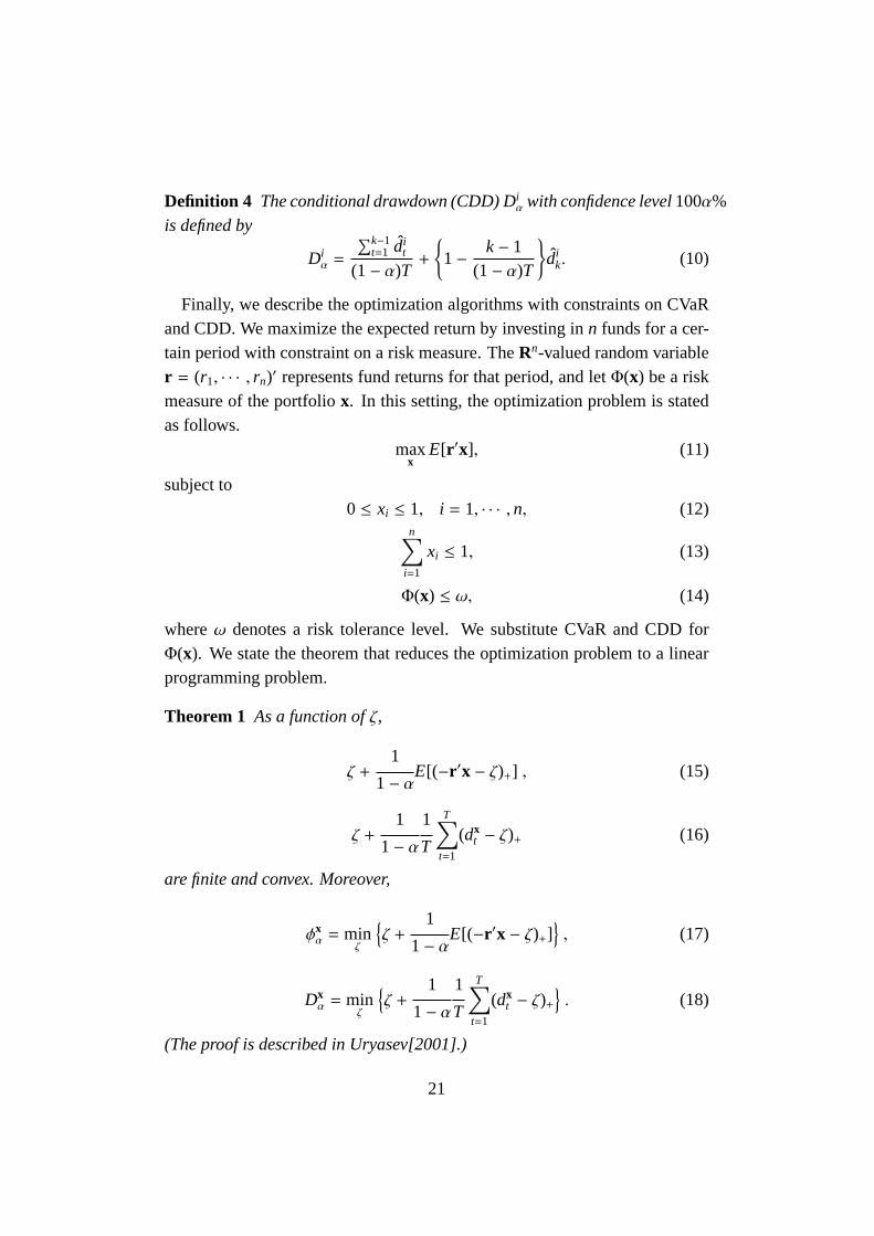
Definition 4 The conditional drawdown (CDD) Diα with confidence level100α%is defined by

Diα =

∑k−1t=1 d̂i

t

(1− α)T +{

1− k− 1(1− α)T

}d̂i

k. (10)

Finally, we describe the optimization algorithms with constraints on CVaRand CDD. We maximize the expected return by investing inn funds for a cer-tain period with constraint on a risk measure. TheRn-valued random variabler = (r1, · · · , rn)′ represents fund returns for that period, and letΦ(x) be a riskmeasure of the portfoliox. In this setting, the optimization problem is statedas follows.

maxx

E[r ′x], (11)

subject to0 ≤ xi ≤ 1, i = 1, · · · ,n, (12)

n∑i=1

xi ≤ 1, (13)

Φ(x) ≤ ω, (14)

whereω denotes a risk tolerance level. We substitute CVaR and CDD forΦ(x). We state the theorem that reduces the optimization problem to a linearprogramming problem.

Theorem 1 As a function ofζ,

ζ +1

1− αE[(−r ′x − ζ)+] , (15)

ζ +1

1− α1

T

T∑t=1

(dxt − ζ)+ (16)

are finite and convex. Moreover,

φxα = min

ζ

{ζ +

1

1− αE[(−r ′x − ζ)+]}, (17)

Dxα = min

ζ

{ζ +

1

1− α1

T

T∑t=1

(dxt − ζ)+

}. (18)

(The proof is described in Uryasev[2001].)

21

By theorem 1, when we haveT historical data, for the case of the CVaRoptimization, the equations (11) and (14) can be expressed as follows.

maxx

1

T

T∑t=1

r ′tx, (19)

ζ +1

1− α1

T

T∑t=1

(−r ′tx − ζ)+ ≤ ω, ζ ∈ R. (20)

Here r t denotes the returns of funds at timet. Because we can rewrite theequation (20) as follows, the CVaR optimization problem can be reduced to alinear programming problem.

ζ +1

1− α1

T

T∑t=1

wt ≤ ω, (21)

−r ′tx − ζ ≤ wt, t = 1, · · · ,T, (22)

ζ ∈ R, wt ≥ 0, t = 1, · · · ,T. (23)

For the case of the CDD optimization, the equations (11) and (14) can beexpressed as follows.

maxx

1

T

T∑t=1

r ′tx, (24)

ζ +1

1− α1

T

T∑t=1

(max1≤s≤T

s∑τ=1

r ′τx −t∑τ=1

r ′τx − ζ)+ ≤ ω, ζ ∈ R. (25)

Because we can rewrite the equation (25) as follows, the CDD optimizationproblem can be reduced to a linear programming problem.

ζ +1

1− α1

T

T∑t=1

zt ≤ ω, (26)

zt ≥ ut −t∑τ=1

r ′τx − ζ, 1 ≤ t ≤ T, (27)

zt ≥ 0, 1 ≤ t ≤ T, (28)

ut ≥t∑τ=1

r ′τx, 1 ≤ t ≤ T, (29)

ut ≥ ut−1, 1 ≤ t ≤ T, (30)

u0 = 0. (31)

22

ReferencesC. Ackermann, R. McEnally, and D. Ravenscraft. ”The Performance ofHedge Funds: Risk, Return, and Incentives”.The Journal of Finance,Vol.54:pp. 833–874, (1999).

V. Agarwal, N.D. Daniel, and N.Y. Naik. ”Role of Managerial Incentives andDiscretion in Hedge Fund Performance”.Working Paper, London Business

School, (2007).

V. Agarwal and N. Y. Naik. ”On Taking the Alternative Route: Risks, Re-wards, and Performance Persistence of Hedge Funds”.Journal of Alternative

Investments, Vol.2:pp. 6–23, (2000a).

V. Agarwal and N. Y. Naik. ”Multi-Period Performance Persistence Analysisof Hedge Funds”.Journal of Financial and Quantitative Analysis, Vol.35:pp.327–342, (2000b).

V. Agarwal and N. Y. Naik. ”Risks and Portfolio Decisions Involving HedgeFunds”.The Review of Financial Studies, Vol.17:pp. 63–98, (2004).

N. Amenc and L. Martellini. ”Portfolio Optimization and Hedge Fund StyleAllocation Decisions”.Journal of Alternative Investments, Vol.5:pp. 7–20,(2002).

G.S. Amin and H.M. Kat. ”Diversification and Yield Enhancement withHedge Funds”.Journal of Alternative Investments, Vol.5:pp. 50–58, (2002).

G.S. Amin and H.M. Kat. ”Hedge Fund Performance 1990-2000: Do the‘ Money Machines’ Really Add Value?”.Journal of Financial and Quanti-

tative Analysis, Vol.38:pp. 251–274, (2003a).

G.S. Amin and H.M. Kat. ”Welcome to the Dark Side: Hedge Fund Attritionand Survivorship Bias over the Period 1994-2001”.Journal of AlternativeInvestments, Vol.6:pp. 57–73, (2003b).

P. Artzner, Delbaen F., Elber, J. M ., and D. Heath. ”Coherent Measures ofRisk”. Mathematical Finance, Vol.9:pp. 203–228, (1999).

23

C. Brooks and H.M. Kat. ”The Statistical Properties of Hedge Fund IndexReturns and Their Implications for Investors”.Journal of Alternative Invest-

ments, Vol.5:pp. 25–44, (2002).

S. Brown and W. Goetzmann. ”Hedge Funds with Style”.Journal of Portfolio

Management, Vol.29:pp. 101–112, (2003).

S. J. Brown, W. N. Goetzmann, and R. G. Ibbotson. ”Offshore Hedge Funds:Survival and Performance 1989-1995”.The Journal of Business, Vol.72:pp.91–117, (1999).

M. K. Brunnermeier and S. Nagel. ”Hedge Funds and the Technology Bub-ble”. The Journal of Finance, Vol.59:pp. 2013–2040, (2004).

A Chekhlov, S.Uryasev, and M. Zabarankin. ”Portfolio Optimization withDrawdown Constraints”. Research Report 2000-5. ISE Dept., Univ. of

Florida, (2000).

J. Cvitanic, L. Martellini A. Lazrak, and F. Zapatero. ”Optimal Allocationto Hedge Funds: an Empirical Analysis”.Quantitative Finance, 3:pp. 1–12,(2003).

R. Davies, H. Kat, and S. Lu. ”Higher Moment Portfolio Analysis withHedge Funds”.Working Paper, ISMA Centre, (2003).

R. Davies, H. Kat, and S. Lu. ”Fund of Hedge Funds Portfolio Selection: AMultiple-Objective Approach”.Working Paper, ISMA Centre, (2004).

F. R. Edwards and M. Caglayan. ”Hedge Funds and Commodity Fund In-vestments in Bull and Bear Markets”.Journal of Portfolio Management,Vol.27:pp. 97–108, (2001).

W. Fung and D. A. Hsieh. ”Empirical Characteristics of Dynamic Trad-ing Strategies: The Case of Hedge Funds”.Review of Financial of Studies,Vol.10:pp. 275–302, (1997).

W. Fung and D. A. Hsieh. ”A Primer on Hedge Funds”.Journal of EmpiricalFinance, Vol.6:pp. 309–331, (1999).

24

W. Fung and D. A. Hsieh. ”Performance Characteristics of Hedge Fundsand CTA Funds: Natural Versus Spurious Biases”.Journal of Financial and

Quantitative Analysis, Vol.35:pp. 291–307, (2000).

W. Fung and D. A. Hsieh. ”The Risk in Hedge Fund Strategies: Theory andEvidence from Trend Followers”.Review of Financial of Studies, Vol.14:pp.313–341, (2001).

W. Fung and D. A. Hsieh. ”Asset-Based Style Factors for Hedge Funds”.Financial Analysts Journal, Vol.58:pp. 16–27, (2002a).

W. Fung and D. A. Hsieh. ”The Risk in Fixed-Income Hedge Fund Styles”.Journal of Fixed Income, Vol.12:pp. 6–27, (2002b).

W. Fung and D. A. Hsieh. ”The Risk in Hedge Fund Strategies: Theoryand Evidence from Long/Short Equity Hedge Funds”.Working Paper, Duke

University, (2006).

D. Kao. ”Battle for Alphas: Hedge Funds versus Long-Only Portfolios”.Financial Analysts Journal, Vol.58:pp. 16–36, (2002).

P. D. Kaplan and J. A. Knowles. ”Kappa: A Generalized Downside Risk-Adjusted Performance Measure”.Journal of Performance Measurement,Vol.8, (2004).

H. Kazemi, T. Schneeweis, and R. Gupta. ”Omega as a Performance Mea-sure”. Working Paper, CISDM, (2003).

F. Koh, W.T.H. Koh, and M. Teo. ”Asian Hedge Funds: Return Persistence,Style and Fund Characteristics”.Working Paper, Singapore ManagementUniversity, (2003).

P. Krokhma, Uryasev, and G. Zrazhevszky. ”Risk Management for HedgeFund Portfolios”. Journal of Alternative Investments, Vol.5:pp. 10–30,(2002).

R. M. Lamm. ”Asymmetric Returns and Optimal Hedge Fund Portfolios”.Journal of Alternative Investments, Vol.6:pp. 9–21, (2003).

B. Liang. ”On the Performance of Hedge Funds”.Financial Analysts Jour-

nal, Vol.55:pp. 72–85, (1999).

25

B. Liang. ”Hedge Funds: The Living and the Dead”.Journal of Financial

and Quantitative Analysis, Vol.35:pp. 309–326, (2000).

B. Liang. ”Hedge Fund Performance: 1990-1999”.Financial Analysts Jour-

nal, (2001).

A. Lo. ”Risk Management for Hedge Funds: Introduction and Overview”.Financial Analysts Journal, Vol.57:pp. 16–33, (2001).

B.G. Malkiel and A. Saha. ”Hedge Funds: Risk and Return”.Financial

Analysts Journal, Vol.61:pp. 80–88, (2005).

R.T. Rockafellar and S.Uryasev. ”Optimization of Conditional Value-at-Risk”. Journal of Risk, Vol.2:pp. 21–41, (2000).

R.T. Rockafellar and S.Uryasev. ”Conditional Value-at-Risk for GenaralLoss Distributions”. Journal of Banking and Finance, Vol.26:pp. 1443–1471, (2002).

T Schneeweis. ”Dealing with Myths of Hedge Fund Investment”.Journal ofAlternative Investments, Vol.1:pp. 11–15, (1998).

T. Schneeweis and R. Spurgin. ”Multifactor Analysis of Hedge Fund, Man-aged Futures, and Mutual Fund Return and Risk Characteristics”.Journal of

Alternative Investments, Vol.1:pp. 1–24, (1998).

F. Sortino and L. Price. ”Performance Measurement in a Downside RiskFramework”.Journal of Investing, pages pp. 59–65, (2001).

26

EXHIBIT 1: Breakdown of Hedge Funds by Investment Strategy and Geog-raphy

27

Number of Funds Average StandardSkew Kurtosis

D-Pin our sample Return Deviation p-value

Investment StrategyLong / Short Equities 58 1.30% 3.85% 0.46 5.21 0.96%Multi-Strategy 17 1.01% 3.25% 0.10 4.75 1.37%CTA /Managed Futures 6 0.63% 4.42% 0.33 4.12 7.95%Relative Value 6 1.30% 4.63% 0.39 4.68 0.45%Distressed Debt 5 1.15% 1.44% −0.14 4.86 0.47%Macro 5 1.80% 9.24% 0.28 5.79 35.14%Fixed Income 4 1.38% 2.00% 1.22 8.22 0.00%Arbitrage 3 0.49% 1.32% −0.36 3.64 19.93%Event Driven 2 1.77% 1.56% 0.80 6.15 0.03%Others 2 1.66% 12.11% 0.20 3.19 61.43%

Investment GeographyJapan Only 26 1.08% 3.59% 0.70 5.35 0.19%Asia incl Japan 21 1.26% 3.76% 0.54 4.75 1.37%Global 20 1.01% 3.90% 0.07 4.63 7.95%Asia ex-Japan 15 1.37% 4.58% 0.27 6.23 0.45%Emerging Markets 13 1.60% 3.81% 0.44 5.75 0.47%Australia/ New Zealand 8 0.96% 2.85% −0.12 3.70 35.14%Korea 2 1.96% 6.03% 0.32 3.56 25.87%Greater China 1 2.17% 7.32% 0.14 2.98 83.87%India 1 2.13% 9.54% −0.98 4.86 0.07%Taiwan 1 0.78% 5.75% −0.17 6.98 0.22%

Asset ClassHedge Fund Universe 108 1.23% 3.94% 0.36 5.10 1.76%Asia-Pacific Stock Indices 37 0.83% 5.22% −0.13 3.03 81.2%Asia-Pacific Bond Indices 9 0.52% 1.22% −0.32 4.75 3.71%

EXHIBIT 2: Statistics for Hedge Fund Categories, 2001-2005

28

EXHIBIT 3: Risk to Return of the Hedge Funds

29

Risk Tolerance Levels 0.10% 0.50% 1.00% 3.00% 5.00%

FUND18 0.39% 2.13% 4.01% 7.05% 10.58%FUND23 2.12% 4.76% 11.17% 20.12% 28.72%FUND72 4.39% 12.36% 12.27% 28.30% 41.77%FUND98 93.10% 80.76% 72.55% 44.53% 18.94%

Expected Returns 2.81% 2.85% 2.88% 2.97% 3.05%Standard Deviations 1.89% 2.12% 2.58% 4.04% 5.60%

CVaR(confidence level 90%) 0.10% 0.50% 1.00% 3.00% 5.00%CDD(confidence level 90%) 0.44% 0.65% 1.21% 3.69% 8.15%

EXHIBIT 4: CVaR (confidence level of 90%) Optimal Portfolios

30

Risk Tolerance Levels 0.10% 0.50% 1.00% 5.00% 10.00%

FUND13 17.84% 0.00% 0.00% 0.00% 0.00%FUND18 0.00% 0.00% 2.97% 3.31% 8.96%FUND23 5.01% 3.28% 10.94% 27.22% 44.26%FUND29 1.86% 0.00% 0.00% 0.00% 0.00%FUND49 1.59% 0.00% 0.00% 0.00% 0.00%FUND72 0.00% 9.16% 10.90% 32.08% 31.38%FUND73 11.69% 0.00% 0.00% 0.00% 0.00%FUND79 2.29% 0.00% 0.00% 0.00% 0.00%FUND88 0.00% 0.00% 0.00% 0.00% 14.00%FUND91 3.59% 0.00% 0.00% 0.00% 0.00%FUND98 56.13% 87.56% 75.19% 37.38% 1.40%

Expected Returns 2.43% 2.83% 2.88% 3.00% 3.10%Standard Deviations 1.75% 1.95% 2.51% 4.88% 7.01%

CVaR(confidence level 90%) 0.10% 0.33% 0.97% 4.26% 7.60%CDD(confidence level 90%) 0.10% 0.50% 1.00% 5.00% 10.00%

EXHIBIT 5: CDD (confidence level of 90%) Optimal Portfolios31

A: Mean-CVaR

B: Mean-Standard Deviation

EXHIBIT 6: Hedge Funds Selected by CVaR or Mean-Variance OptimizationPrograms

32

・A: Mean-CDD

B: Mean-Standard Deviation

EXHIBIT 7: Hedge Funds Selected by CDD or Mean-Variance OptimizationPrograms

33

Expected Returns 1.50% 2.43% 2.81%

Standard Deviations 0.61% 1.38% 1.86%CVaR(confidence level 90%) -0.39% -0.23% 0.21%CDD(confidence level 90%) 0.05% 0.32% 0.49%

EXHIBIT 8: Statistics for Mean-Variance Optimal Portfolios

EXHIBIT 9: Growth in Wealth Managed by Optimal Portfolios

34

EXHIBIT 10: Transfers of Weights Allocated to each fund within the CDD(risk tolerance level at 0.1%) Optimal Portfolio

35

Risk Tolerance Levels 0.10% 0.50% 1.00% 2.00% 3.00% 4.00% 5.00%

Annualized Returns 23.40% 21.92% 20.43% 17.49% 13.93% 10.67% 7.36%Standard Deviations 4.87% 4.72% 4.63% 4.59% 4.91% 5.34% 5.87%

Sharpe ratios 4.31 4.13 3.90 3.29 2.35 1.55 0.85maximum drawdowns 1.68% 1.54% 1.42% 2.02% 2.98% 3.76% 4.63%

CVaR(Confidence Level 90% ) 1.22% 1.18% 1.11% 1.19% 1.41% 1.79% 2.20%CDD(Confidence Level 90% ) 1.43% 1.41% 1.29% 1.63% 2.07% 2.55% 3.73%

A: CVaR Optimal Portfolio

risk tolerance levels 0.10% 0.50% 1.00% 3.00% 5.00% 7.00% 10.00%

annualized returns 24.04% 23.12% 20.98% 17.81% 16.49% 15.50% 13.10%standard deviations 4.94% 4.89% 5.03% 4.64% 4.52% 4.46% 5.15%


CVaR(confidence level 90% ) 1.14% 1.23% 1.47% 1.30% 1.16% 1.11% 1.49%CDD(confidence level 90% ) 1.19% 1.47% 2.30% 2.39% 2.14% 1.83% 2.33%

B: CDD Optimal Portfolio

expected returns 1.00% 1.50% 2.00% 2.50% 3.00% CVaR0.1% CDD0.1%




C: Mean-Variance Optimal Portfolio

EXHIBIT 11: Performances of the Optimal Portfolios, 2004-2005

36





A: CVaR Optimal Portfolio





B: CDD Optimal Portfolio

expected returns 1.50% 2.00% 2.50% 3.00%

annualized returns 12.49% 14.29% 12.79% 11.95%standard deviations 2.75% 4.07% 5.31% 5.43%

Sharpe ratios 3.68 2.92 1.96 1.76maximum drawdowns 0.85% 1.89% 4.28% 4.01%

CVaR(confidence level 90% ) 0.52% 0.93% 1.72% 2.07%CDD(confidence level 90% ) 0.72% 1.74% 3.91% 3.70%

C: Mean-Variance Optimal Portfolio

EXHIBIT 12: Performances of the Optimal Portfolios with 15% Limitations,2004-2005

37

Stock IndicesJapan Russell/Nomura Large Cap Growth Index With Dividend New Zealand NZSE NZX ALL INDEX

Russell/Nomura Large Cap Index With Dividend NZSEG NZX ALL GROSS INDEXRussell/Nomura Large Cap Value Index With Dividend NZSE10 NZX TOP 10 INDEXRussell/Nomura Mid Cap Growth Index With Dividend NZSEMC NZX MID CAP INDEXRussell/Nomura Mid Cap Index With Dividend NZSESC NZX SMALLCAP INDEXRussell/Nomura Mid Cap Value Index With Dividend Philippines PASHR PHILIPPINES ALL SHARE IXRussell/Nomura Mid-Small Cap Growth Index With Dividend PCOMP PHILIPPINES COMPOSITE IXRussell/Nomura Mid-Small Cap Index With Dividend SME PHILIPPINES SM-MED ENTERRussell/Nomura Mid-Small Cap Value Index With Dividend Singapore BTSRI SING: BUSINESS TIME REGNRussell/Nomura Small Cap Growth Index With Dividend SESALL SINGAPORE ALL INDEXRussell/Nomura Small Cap Index With Dividend STI STRAITS TIMES INDEXRussell/Nomura Small Cap Value Index With Dividend UOBDAQ SING: UOB SESDAQ INDEXRussell/Nomura Top Cap Growth Index With Dividend South Korea KRX100 KOREA EXCHANGE 100 INDEXRussell/Nomura Top Cap Index With Dividend KOSPI KOREA COMPOSITE INDEXRussell/Nomura Top Cap Value Index With Dividend KOSPI2 KOREA KOSPI 200 INDEXRussell/Nomura Total Market Growth Index With Dividend KOSDAQ KOSDAQ COMPOSITE INDEXRussell/Nomura Total Market Index With Dividend KOSPI100 KOREA KOSPI 100 INDEXRussell/Nomura Total Market Value Index With Dividend KOSPI50 KOREA KOSPI 50 INDEX

Australia AS25 S&P/ASX 100 INDEX KOSPLMKC KOSPI LARGE CAP INDEXAS26 S&P/ASX 20 INDEX KOSPMMKC KOSPI MID CAP INDEXAS31 S&P/ASX 50 INDEX KOSPSMKC KOSPI SMALL CAP INDEXAS34 S&P/ASX MIDCAP 50 INDEX KOSTAR KOSDAQ STAR INDEXAS38 S&P/ASX SMALL ORDS INDEX KOSDAQ50 KOSDAQ50 INDEXAS39 ASX SMALLCAP RESOURCES KOSD100 KOSDAQ 100 INDEXAS40 ASX SMALLCAP INDUSTRIALS KOSDM300 KOSDAQ MID300 INDEXAS51 S&P/ASX 200 INDEX KOSDSMAL KOSDAQ SMALL INDEXAS52 S&P/ASX 300 INDEX Taiwan TWSE TAIWAN TAIEX INDEX

Shenzen SZASHR CHINA SE SHENZHEN A TW50 TSEC TAIWAN 50 INDEXSZBSHR CHINA SE SHENZHEN B TWMC TSEC MID-CAP 100 INDEXSZCOMP CHINA SE SHENZ COMPOSITE TWIT TSEC TECHNOLOGY INDEXSIASA SSE A-SHARE INDEX TWOTCI TAIWAN GRE TAI EXCHANGESIBSB SSE B-SHARE INDEX Thailand SET STOCK EXCH OF THAI INDEXSICOM SSE CONSTITUENT STOCK IX SET50 THAI SET 50 INDEXSHSZ300 SHSE-SZSE300 INDEX MAI THAI STOCK EXCHG MAI IXFXTID FTSE/XINHUA CHINA 25 SET100 THAI SET 100 INDEXXIN3I FTSE XINHUA CH A200 INDX Bangladesh DHAKA DHAKA STK EXG DHAKA EXCHXIN5I FTSE XINHUA CH A400 INDX India BSE100 BOMBAY STOCK EX 100 IDX

Shanghai SHASHR CHINA SE SHANGHAI A BSE200 BOMBAY STOCK EX 200 IDXSHBSHR CHINA SE SHANGHAI B SENSEX BSE SENSEX 30 INDEXSHCOMP CHINA SE SHANG COMPOSITE DOLLEX DOLLEX INDEX DOLLEX IDXSSE180 CHINA SE SHANG 180 A SHR NIFTY NSE S&P CNX NIFTY INDEXSSE50 SHANGHAI SE 50 A-SHR IDX DOLL30 DOLLEX INDEX DOLL BSE30SHSZ300 SHSE-SZSE300 INDEX BSE500 BOMBAY STOCK EX 500 IDX

Hong Kong HKX AMEX HONG KONG 30 INDEX DEFTY NSE S&P CNX DEFTY INDEXHSI HANG SENG INDEX BSEMDCAP BSE MID-CAP INDEXHSHKLI HANG SENG HK LARGE CAP BSESMCAP BSE SMALL-CAP INDEXHSHKMI HANG SENG HK MID CAP IDX NIFTYJR NSE S&P CNX MIDCAP INDEXHSHKSI HANG SENG HK SMALL CAP CNXBANK BANK NIFTY INDEXHKSPLC25 S&P/HKEx LargeCap Index CNXMCAP NSE CNX MIDCAP INDEXHKSPGEM S&P/HKEx GEM Index FTY1ID FTSE World India

Jakarta JCI JAKARTA COMPOSITE INDEX Pakistan KSE Pakistan All ShareMBX JAKARTA SE MAIN BOARD IX KSE100 PAKISTAN 100 INDEXDBX JAKARTA SE DEVEL BRD IDX Sri Lanka CSEALL Sri Lanka All ShareLQ45 JAKARTA LQ-45 INDEX the US S&P 500D300IN HSBC Dragon INDONESIA Europe Dow-Jones European stock indexJAKISL JAKARTA ISLAMIC INDEX

Surabaya SSXCSPI SSX CSPIMalaysia KLSI KUALA LUMPUR SYARIAH IX

KL2ND KUALA LUMPUR 2ND BOARDKLCI KUALA LUMPUR COMP INDEXMCI MESDAQ COMPOSITE INDEX

CurrenciesBond Indices Japanese YenMSCI Australia TR EuroMSCI Japan TR Singapore DollarMSCI New Zealand TR South Korea WonMSCI US Treasury TR Taiwanese DollarMSCI Hong Kong Dollar Swap TR Hong Kong DollarMACI Indonesia Rupiah Swap TR Thai BuhtMSCI Phlippines Peso Swap TR Malaysia RinggitMSCI Singapore Dollar Swap TR Indonesian RupiahMSCI South Korea Won Swap TR Australian DollarMSCI Thailand Baht Swap TR New Zealand DollarMSCI Taiwan Dollar Swap TR Indian Rupee

Philippenes PesoChina Yuan

EXHIBIT 13: Market Indices

38

investment Distressed Relative Long / Short Fixed Multi-Macro

CTA / Eventstrategies Debt Value Equities Income Strategy Managed Futures Driven

number of funds4 3 18 3 4 3 3 1

(total 39)

average adjusted0.45 0.37 0.58 0.50 0.39 0.32 0.35 0.38

R2(entire)


R2(first half)


R2(latter half)

A: Results for Investment Strategies

investment Asia AsiaKorea Global

Emerging Greater Australia/ Japangeographies ex-Japan incl Japan Markets China New Zealand Only

number of funds7 7 2 8 5 1 2 7

(total 39)


R2(entire)


R2(first half)


R2(latter half)

B: Results for Investment Geography

EXHIBIT 14: Regression Results for Investment Strategies and InvestmentGeography

39

A: Increases in Wealths of the CDD Optimal Portfolio (risk tolerance level0.1%) and its Mimicking Portfolio

B: Returns of the Single Hedge Funds and Their Mimicking Portfolios

EXHIBIT 15: Results of Return Replications

Documents

Selection and Performance Analysis of Asia-Paciﬁc …park.itc.u-tokyo.ac.jp/takahashi-lab/WPs/p17.pdf · Selection and Performance Analysis of ... Many researchers have tried to