Embed Size (px)
Citation preview
International Journal of Advance Engineering and Research Development (IJAERD)
Volume 1,Issue 5,May 2014, e-ISSN: 2348 - 4470 , print-ISSN:2348-6406
@IJAERD-2014, All rights Reserved 1
SELECTION OF THE WIRE CUT ELECTRICAL DISCHARGE
MACHINING PROCESS PARAMETERS USING GRA METHOD
Vipal B Patel1*, Jaksan D. Patel2, Kalpesh D. Maniya3
1M.E. student, Sardar Patel Institute of Technology, Piludara, Mehsana, [email protected]
2Head of Mechanical Department at Merchant Polytechnic, Basna, [email protected]
3Asst. Professor, C.K.Pithawalla College of engg. & Technology, Surat, [email protected]
Abstract: Wire electrical discharge machining (WEDM) is one of the important non-traditional machining processes, which is used for machining of difficult-to-machine materials and intricate
profiles. WEDM is a complex machining process controlled by a large number of process parameters such as Pulse on Time (Ton), Pulse off Time (Toff), Flushing Pressure (FP), Wire Tension (Wt),
Servo Voltage (SV) and Wire Feed Rate (WF) in Wire Cut Electrical Discharge Machining (WEDM) Operations. The Response Process Parameters are measure in Wire Cut Electrical Discharge Machining (WEDM) Operations Such as Material Removal Rate, Kerf Width and Surface
Roughness have been considered for Each Experiment. Experimentation was planned as per Taguchi’s L27 Orthogonal array. Molybdenum Wire with 0.25mm Diameter and High Carbon High
Chromium Die Steel (HCHCR) were used as tool and Work Materials in the Experiments. The Machining parameters are optimized with the multi response characteristics of the material removal, kerf width rate and surface roughness using the grey relational analysis.
Keywords: WEDM, Step by Step Procedure of WEDM, Taguchi Method, Orthogonal Array, GRA
I.INTRODUCTION
One of the most widely used Non-Conventional Machining process in industry is Electrical Discharge Machining (EDM)[1]. Electric Discharge Machining is a non- traditional concept which is based on the principle of removing material by means of repeated electrical discharges between the
tool termed as electrode and the work piece in the presence of a dielectric fluid. WEDM is considered as a unique adoption of the conventional EDM process which comprises of a main
worktable, wire drive mechanism, a CNC controller, working fluid tank and attachments. The work piece is placed on the fixture table and fixed securely by clamps and bolts. The table moves along X and Y-axis and it is driven by the DC servo motors. Wire electrode usually made of thin copper,
brass, molybdenum or tungsten of diameter 0.05-0.30 mm, which transforms electrical energy to thermal energy, is used for cutting materials. The wire is stored and wound on a wire drum which
can rotate at1500rpm. The wire is continuously fed from wire drum which moves though the work piece and is supported under tension between a pair of wire guides located at the opposite sides of the work piece. During the WEDM process, the material is eroded ahead of the wire and there is no
direct contact between the work piece and the wire, eliminating the mechanical stresses during machining. Also the work piece and the wire electrode (tool) are separated by a thin film of dielectric
fluid that is continuously fed to the machining zone to flush away the eroded particles. The movement of table is controlled numerically to achieve the desired three-dimensional shape and accuracy of the work piece [1].
A. STEP BY STEP PROCEDUREOFWEDMPROCESS:
Step: 1
International Journal of Advance Engineering and Research Development (IJAERD)
Volume 1,Issue 5,May 2014, e-ISSN: 2348 - 4470 , print-ISSN:2348-6406
@IJAERD-2014, All rights Reserved 2
Generation of Volts and Amps as wire is surrounded by deionized water as shown in figure 1.1
[2].
“Figure: 1.1Volts and Amps produced by power supply [2]”
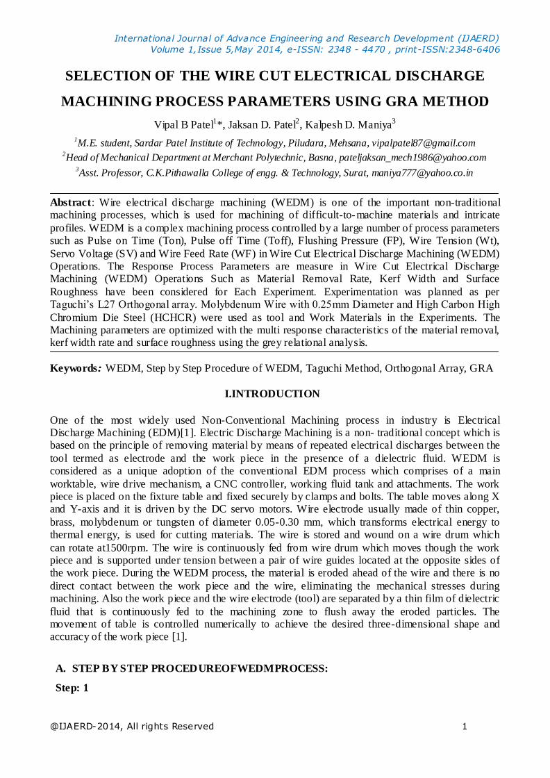
Step: 2
During pulse on time controlled sparks are produced between work piece and electrode which
helps in erosion and hence precisely melts and vaporize the material as shown in figure 1.2.
“Figure: 1.2Sparkgeneration and erosion of material [2]”
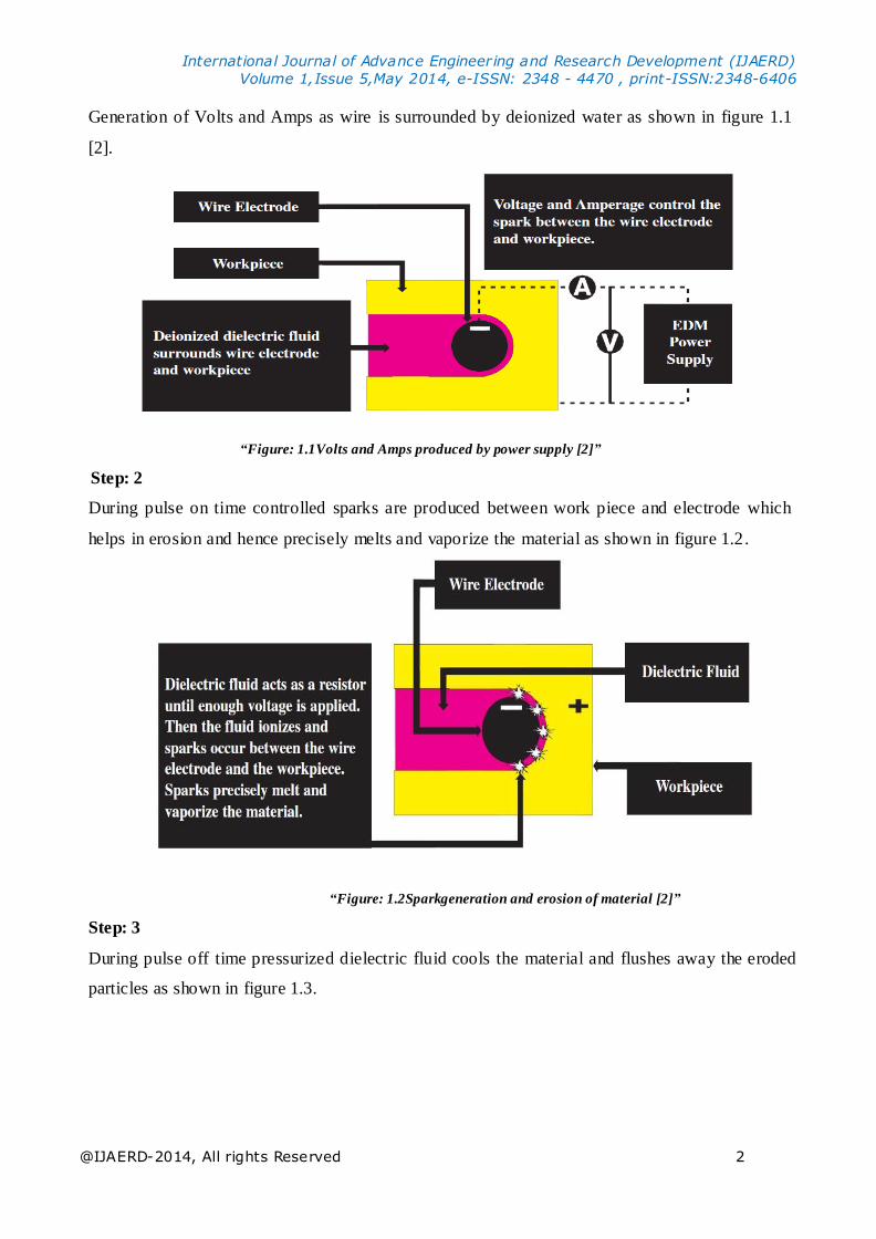
Step: 3
During pulse off time pressurized dielectric fluid cools the material and flushes away the eroded
particles as shown in figure 1.3.
International Journal of Advance Engineering and Research Development (IJAERD)
Volume 1,Issue 5,May 2014, e-ISSN: 2348 - 4470 , print-ISSN:2348-6406
@IJAERD-2014, All rights Reserved 3
“Figure: 1.3Flushingof corroded particles [2]”
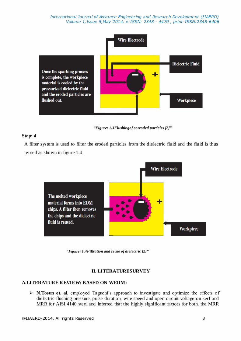
Step: 4
A filter system is used to filter the eroded particles from the dielectric fluid and the fluid is thus
reused as shown in figure 1.4.
“Figure: 1.4Filtration and reuse of dielectric [2]”
II. LITERATURESURVEY
A.LITERATURE REVIEW: BASED ON WEDM:
N.Tosun et. al. employed Taguchi’s approach to investigate and optimize the effects of dielectric flushing pressure, pulse duration, wire speed and open circuit voltage on kerf and MRR for AISI 4140 steel and inferred that the highly significant factors for both, the MRR
International Journal of Advance Engineering and Research Development (IJAERD)
Volume 1,Issue 5,May 2014, e-ISSN: 2348 - 4470 , print-ISSN:2348-6406
@IJAERD-2014, All rights Reserved 4
and the kerf, are open voltage and pulse duration whereas dielectric flushing pressure and
wire speed are less effective factors. It has also concluded that confirmation tests indicated that it is possible to decrease kerf and increase MRR significantly by using the proposed
statistical technique. [3]
Kanlayasiri and Boonmung have investigated influences of wire-EDM machining variables on surface roughness of newly developed DC 53 die steel of width, length, and
thickness 27, 65 and 13 mm, respectively. The machining variables included pulse-on time, pulse-off time, pulse-peak current, and wire tension. The variables affecting the surface roughness were identified using ANOVA technique. Results showed that pulse-on time and
pulse-peak current were significant variables to the surface roughness of wire- EDM DC53 die steel. The maximum prediction error of the model was less than 7% and the average
percentage error of prediction was less than 3%. [4]. B.K. Nanda et. al. have conducted the experiment on Parametric Optimization of CNC Wire
Cut Electrical Discharge Machining using grey relational Analysis. In This Experiment has been performed under different cutting conditions with the grey relational Analysis and
analysis of variance (ANOVA). Grey relational grade using the optimal process parameter combinations and found that a good agreement between the predicted and actual grey relational grade. The increase of grey relational grade from initial factor setting to the op timal
process parameter setting is of 0.1275. It has concluded that optimization of the complicated multiple performance characteristics using gray relation method and obtain the material
removal rate, surface roughness are improved together.[5]
Datta and Mahapatra have proposed a quadratic mathematical model and conducted
experiments by taking six WEDM process parameters: discharge current, pulse duration, pulse frequency, wire speed, wire tension and dielectric flow rate. Experiments were carried
out on D2 Tool Steel using a Zinc coated Copper wire electrode. The response parameters noticed for each experiment were MRR, Surface Roughness and Kerf. A statistical analysis has been carried for each result and responses have been utilized to fit the quadratic model
which represents the above said six parameters. Grey based Taguchi technique has been utilized to evaluate optimal parameter combination to achieve maximum MRR, minimum
roughness value and minimum width of cut; with selected experimental domain. It has been found out that for continuous quality improvement Grey based Taguchi method is a very reliable method to predict optimal parameter values and all the parameters involved in
the experimentation are independent of each other.[6]
Pasam et. al. have developed a mathematical model by using linear regression analysis in order to present a relationship between control parameters and response parameters. Titanium alloy is chosen as work piece material. Control parameters which have been varied are
Ignition pulse current, Short pulse duration, Time between two pulses, Servo speed, Servo voltage, Injection pressure, Wire speed and Wire tension and the response parameter studied
for the above parameters is surface roughness. Genetic algorithm modelling has been used to optimize the process parameters for surface roughness. Regression coefficient of 0.943 is obtained for surface roughness model by regression analysis and surface roughness of 1.85
μm is obtained with selected optimum control parame ters in the WEDM of Ti6Al4V alloy.[7]
Kuo-Wei Lin et. al. have conduct test Wire Electrical Discharge Machining (WEDM) of
magnesium alloy parts via the taguchi method-based gray analysis was conducted; they
International Journal of Advance Engineering and Research Development (IJAERD)
Volume 1,Issue 5,May 2014, e-ISSN: 2348 - 4470 , print-ISSN:2348-6406
@IJAERD-2014, All rights Reserved 5
considered multiple quality characteristics required include material removal rate and surface
roughness following WEDM. Entropy Weighting employs the entropy concept to determine the relative weighting factor for each attribute .This work machines magnesium alloy parts
under controlled machine parameter settings, and measures the above quality characteristics. The optimized machine parameter settings clearly improve quality characteristics of the machined work piece compared to quality levels achieved for initial machine parameter
settings. The complex interactions in WEDM involve wire feed rate, pulse-on time, pulse-off time, no load voltage, servo voltage, and wire tension.[8]
C Bhaskar Reddy et.al. also conducted the experiments in wire EDM based on L16
Orthogonal array selecting EN19 and SS420 steel as work material with 0.18 mm
Molybdenum wire as electrode. The experiments are conducted considering the above two materials for L16 and then the impact of each parameter is estimated by ANOAVA. Then the regression analysis is carried-out to find the trend of the response of each material.
Recommend better parameter settings to achieve higher MRR and better surface roughness. Based on the results; it is recommended that the EN 19 material is suitable for better MRR.
Then the SS 420 material is recommended to obtain better surface. [9].
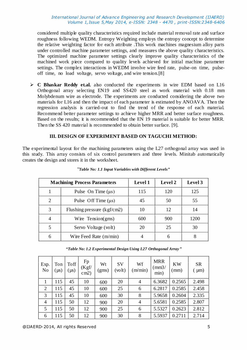
III. DESIGN OF EXPERIMENT BASED ON TAGUCHI METHOD:
The experimental layout for the machining parameters using the L27 orthogonal array was used in this study. This array consists of six control parameters and three levels. Minitab automatically
creates the design and stores it in the worksheet.
“Table No: 1.1 Input Variables with Different Levels”
Machining Process Parameters Level 1 Level 2 Level 3
1 Pulse On Time (μs) 115 120 125
2 Pulse Off Time (μs) 45 50 55
3 Flushing pressure (kgf/cm2) 10 12 14
4 Wire Tension(gms) 600 900 1200
5 Servo Voltage (volt) 20 25 30
6 Wire Feed Rate (m/min) 4 6 8
“Table No: 1.2 Experimental Design Using L27 Orthogonal Array”
Exp.
No
Ton
(µs)
Toff
(µs)
Fp
(Kgf/cm2)
Wt
(gms)
SV
(volt)
Wf
(m/min)
MRR
(mm3/min)
KW
(mm)
SR
( µm)
1 115 45 10 600 20 4 6.3682 0.2565 2.498
2 115 45 10 600 25 6 6.2817 0.2585 2.458
3 115 45 10 600 30 8 5.9658 0.2604 2.335
4 115 50 12 900 20 4 5.6581 0.2585 2.807
5 115 50 12 900 25 6 5.5327 0.2623 2.812
6 115 50 12 900 30 8 5.5937 0.2711 2.714

International Journal of Advance Engineering and Research Development (IJAERD)
Volume 1,Issue 5,May 2014, e-ISSN: 2348 - 4470 , print-ISSN:2348-6406
@IJAERD-2014, All rights Reserved 6
IV.METHODOLOGY: GREY RELATION ANALYSIS (GRA)
In grey relational analysis, the function of factors is neglected in situations where the range of the
sequence is large or the standard value is enormous .However, this analysis might produce incorrect results if the factors ,goal and directions are different .Therefore one has to pre-process the data
which are related to a group of sequence ,which is called “grey relational generation “data preprocessing is a process of transferring the original sequence to a comparable sequence for this purpose the experimental result are normalized in the range between zero and one the normalization
can be done from three different approaches.
A. Data pre-processing
If the target value of original sequence is infinite, then it has a characteristic of “the larger the better”. The original sequence can be normalized as follows [5]:
…………….... Eq.1
If the expectancy is “the smaller the better” than the original sequence should be normalized as
follows:
7 115 55 14 1200 20 4 5.2816 0.2665 2.786
8 115 55 14 1200 25 6 5.1930 0.2724 2.680
9 115 55 14 1200 30 8 5.1124 0.2764 2.763
10 120 45 12 1200 20 6 8.3161 0.2700 3.375
11 120 45 12 1200 25 8 7.9069 0.2677 3.403
12 120 45 12 1200 30 4 7.4141 0.2661 3.370
13 120 50 14 600 20 6 7.1922 0.2702 3.399
14 120 50 14 600 25 8 6.9960 0.2716 3.434
15 120 50 14 600 30 4 7.0043 0.2813 3.417
16 120 55 10 900 20 6 5.8348 0.2589 3.470
17 120 55 10 900 25 8 5.3332 0.2550 3.504
18 120 55 10 900 30 4 5.0727 0.2552 3.388
19 125 45 14 900 20 8 8.4101 0.2623 3.536
20 125 45 14 900 25 4 8.1089 0.2638 3.485
21 125 45 14 900 30 6 8.1004 0.2656 3.450
22 125 50 10 1200 20 8 7.6840 0.2589 3.505
23 125 50 10 1200 25 4 7.4889 0.2616 3.489
24 125 50 10 1200 30 6 7.7415 0.2758 3.429
25 125 55 12 600 20 8 7.2994 0.2759 3.427
26 125 55 12 600 25 4 7.0054 0.2808 3.446
27 125 55 12 600 30 6 7.1029 0.2936 3.399
i(k)-min i(k)i(k) =
max i(k)-min i(k)
y yx y y
International Journal of Advance Engineering and Research Development (IJAERD)
Volume 1,Issue 5,May 2014, e-ISSN: 2348 - 4470 , print-ISSN:2348-6406
@IJAERD-2014, All rights Reserved 7
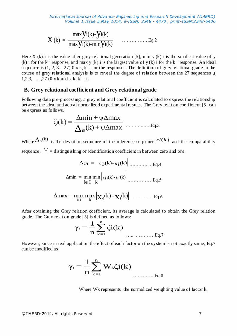
……………. Eq.2
Here X (k) i is the value after grey relational generation [5], min y (k) i is the smallest value of y
(k) i for the kth response, and max y (k) i is the largest value of y (k) i for the kth response. An ideal sequence is (1, 2, 3... 27) 0 x k, k = for the responses. The definition of grey relational grade in the course of grey relational analysis is to reveal the degree of rela tion between the 27 sequences ,(
1,2,3,.......,27) 0 x k and x k, k = i .
B. Grey relational coefficient and Grey relational grade
Following data pre-processing, a grey relational coefficient is calculated to express the relationship between the ideal and actual normalized experimental results. The Grey relation coefficient [5] can be express as follows.
i
0i
Δmin +ψΔmaxζ (k) =
(k) +ψΔmaxΔ………………Eq.3
Where 0( )
ik is the deviation sequence of the reference sequence ( )xi k and the comparability
sequence . ψ = distinguishing or identification coefficient in between zero and one.
Δ = (k)- (k)0i x x0 i ………… …Eq.4
Δmin = min min (k)- (k)x x0 i
i I k .……………Eq.5
0 ii I k
Δmax = maxmax (k) - (k)x x
……………Eq.6
After obtaining the Grey relation coefficient, its average is calculated to obtain the Grey relation
grade. The Grey relation grade [5] is defined as follows: n
i
k=1
1γ = ζi(k)
n
….. .…………Eq.7
However, since in real application the effect of each factor on the system is not exactly same, Eq.7 can be modified as:
n
i k
k=1
1γ = W ζi(k)
n
…………..Eq.8
Where Wk represents the normalized weighting value of factor k.
max i(k)- i(k)i(k) =
max i(k)-min i(k)
y yx y y
International Journal of Advance Engineering and Research Development (IJAERD)
Volume 1,Issue 5,May 2014, e-ISSN: 2348 - 4470 , print-ISSN:2348-6406
@IJAERD-2014, All rights Reserved 8
In Grey relation analysis, the grey relation grade is used to show the relationship among the
sequences. If the two sequences are identical, then the value of Grey relation grade is equal to 1.The Grey relation grade also indicates the degree of influence that the comparability sequence
could exert over the reference sequence. Therefore, if a particular comparability sequence is more important than the other comparability sequence to reference sequence will be higher than other grey relation grades. In this study, the importance of both the comparability sequence and
reference sequence is treated as equal.
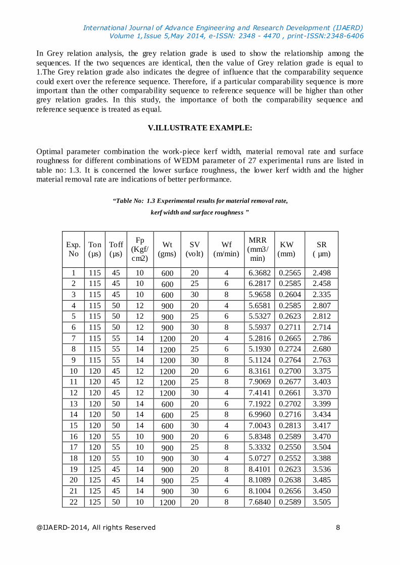
V.ILLUSTRATE EXAMPLE:
Optimal parameter combination the work-piece kerf width, material removal rate and surface roughness for different combinations of WEDM parameter of 27 experimenta l runs are listed in
table no: 1.3. It is concerned the lower surface roughness, the lower kerf width and the higher material removal rate are indications of better performance.
“Table No: 1.3 Experimental results for material removal rate,
kerf width and surface roughness ”
Exp.No
Ton (µs)
Toff (µs)
Fp (Kgf/cm2)
Wt (gms)
SV (volt)
Wf (m/min)
MRR (mm3/min)
KW (mm)
SR ( µm)
1 115 45 10 600 20 4 6.3682 0.2565 2.498
2 115 45 10 600 25 6 6.2817 0.2585 2.458
3 115 45 10 600 30 8 5.9658 0.2604 2.335
4 115 50 12 900 20 4 5.6581 0.2585 2.807
5 115 50 12 900 25 6 5.5327 0.2623 2.812
6 115 50 12 900 30 8 5.5937 0.2711 2.714
7 115 55 14 1200 20 4 5.2816 0.2665 2.786
8 115 55 14 1200 25 6 5.1930 0.2724 2.680
9 115 55 14 1200 30 8 5.1124 0.2764 2.763
10 120 45 12 1200 20 6 8.3161 0.2700 3.375
11 120 45 12 1200 25 8 7.9069 0.2677 3.403
12 120 45 12 1200 30 4 7.4141 0.2661 3.370
13 120 50 14 600 20 6 7.1922 0.2702 3.399
14 120 50 14 600 25 8 6.9960 0.2716 3.434
15 120 50 14 600 30 4 7.0043 0.2813 3.417
16 120 55 10 900 20 6 5.8348 0.2589 3.470
17 120 55 10 900 25 8 5.3332 0.2550 3.504
18 120 55 10 900 30 4 5.0727 0.2552 3.388
19 125 45 14 900 20 8 8.4101 0.2623 3.536
20 125 45 14 900 25 4 8.1089 0.2638 3.485
21 125 45 14 900 30 6 8.1004 0.2656 3.450
22 125 50 10 1200 20 8 7.6840 0.2589 3.505
International Journal of Advance Engineering and Research Development (IJAERD)
Volume 1,Issue 5,May 2014, e-ISSN: 2348 - 4470 , print-ISSN:2348-6406
@IJAERD-2014, All rights Reserved 9
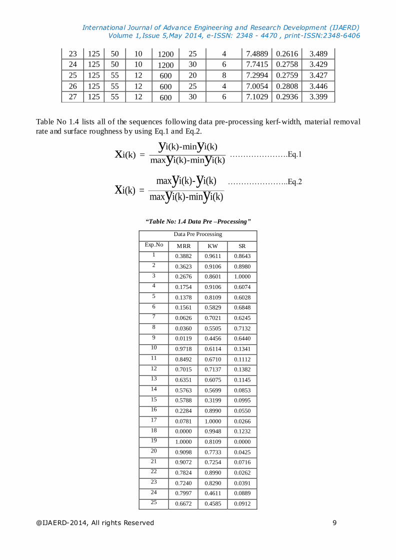
Table No 1.4 lists all of the sequences following data pre-processing kerf-width, material removal
rate and surface roughness by using Eq.1 and Eq.2.
………………….Eq.1
…………………..Eq.2
“Table No: 1.4 Data Pre –Processing”
23 125 50 10 1200 25 4 7.4889 0.2616 3.489
24 125 50 10 1200 30 6 7.7415 0.2758 3.429
25 125 55 12 600 20 8 7.2994 0.2759 3.427
26 125 55 12 600 25 4 7.0054 0.2808 3.446
27 125 55 12 600 30 6 7.1029 0.2936 3.399
Data Pre Processing
Exp.No MRR KW SR
1 0.3882 0.9611 0.8643
2 0.3623 0.9106 0.8980
3 0.2676 0.8601 1.0000
4 0.1754 0.9106 0.6074
5 0.1378 0.8109 0.6028
6 0.1561 0.5829 0.6848
7 0.0626 0.7021 0.6245
8 0.0360 0.5505 0.7132
9 0.0119 0.4456 0.6440
10 0.9718 0.6114 0.1341
11 0.8492 0.6710 0.1112
12 0.7015 0.7137 0.1382
13 0.6351 0.6075 0.1145
14 0.5763 0.5699 0.0853
15 0.5788 0.3199 0.0995
16 0.2284 0.8990 0.0550
17 0.0781 1.0000 0.0266
18 0.0000 0.9948 0.1232
19 1.0000 0.8109 0.0000
20 0.9098 0.7733 0.0425
21 0.9072 0.7254 0.0716
22 0.7824 0.8990 0.0262
23 0.7240 0.8290 0.0391
24 0.7997 0.4611 0.0889
25 0.6672 0.4585 0.0912
i(k)-min i(k)i(k) =
max i(k)-min i(k)
y yx y y
max i(k)- i(k)i(k) =
max i(k)-min i(k)
y yx y y
International Journal of Advance Engineering and Research Development (IJAERD)
Volume 1,Issue 5,May 2014, e-ISSN: 2348 - 4470 , print-ISSN:2348-6406
@IJAERD-2014, All rights Reserved 10
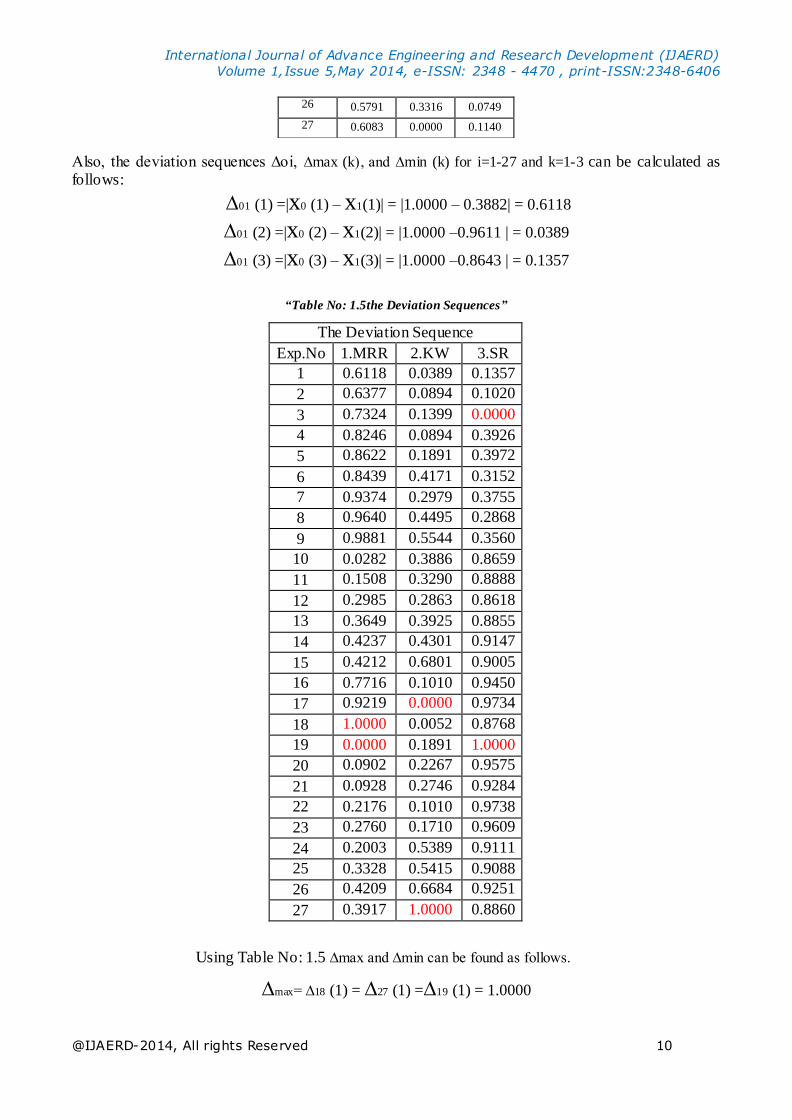
Also, the deviation sequences ∆oi, ∆max (k), and ∆min (k) for i=1-27 and k=1-3 can be calculated as follows:
∆01 (1) =|x0 (1) – x1(1)| = |1.0000 – 0.3882| = 0.6118
∆01 (2) =|x0 (2) – x1(2)| = |1.0000 –0.9611 | = 0.0389
∆01 (3) =|x0 (3) – x1(3)| = |1.0000 –0.8643 | = 0.1357
“Table No: 1.5the Deviation Sequences”
The Deviation Sequence
Exp.No 1.MRR 2.KW 3.SR
1 0.6118 0.0389 0.1357
2 0.6377 0.0894 0.1020
3 0.7324 0.1399 0.0000
4 0.8246 0.0894 0.3926
5 0.8622 0.1891 0.3972
6 0.8439 0.4171 0.3152
7 0.9374 0.2979 0.3755
8 0.9640 0.4495 0.2868
9 0.9881 0.5544 0.3560
10 0.0282 0.3886 0.8659
11 0.1508 0.3290 0.8888
12 0.2985 0.2863 0.8618
13 0.3649 0.3925 0.8855
14 0.4237 0.4301 0.9147
15 0.4212 0.6801 0.9005
16 0.7716 0.1010 0.9450
17 0.9219 0.0000 0.9734
18 1.0000 0.0052 0.8768
19 0.0000 0.1891 1.0000
20 0.0902 0.2267 0.9575
21 0.0928 0.2746 0.9284
22 0.2176 0.1010 0.9738
23 0.2760 0.1710 0.9609
24 0.2003 0.5389 0.9111
25 0.3328 0.5415 0.9088
26 0.4209 0.6684 0.9251
27 0.3917 1.0000 0.8860
Using Table No: 1.5 ∆max and ∆min can be found as follows.
∆max= ∆18 (1) = ∆27 (1) =∆19 (1) = 1.0000
26 0.5791 0.3316 0.0749
27 0.6083 0.0000 0.1140
International Journal of Advance Engineering and Research Development (IJAERD)
Volume 1,Issue 5,May 2014, e-ISSN: 2348 - 4470 , print-ISSN:2348-6406
@IJAERD-2014, All rights Reserved 11
∆min = ∆19 (1) =∆17 (1) = ∆03 (1) = 0.0000
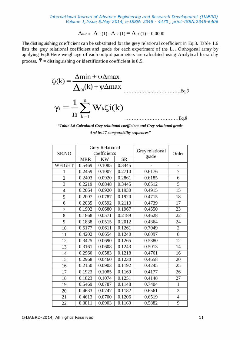
The distinguishing coefficient can be substituted for the grey relational coefficient in Eq.3. Table 1.6
lists the grey relational coefficient and grade for each experiment of the L27 Orthogonal array by applying Eq.8.Here weightage of each output parameters are calculated using Analytical hierarchy
process. ψ= distinguishing or identification coefficient is 0.5.
i
0i
Δmin +ψΔmaxζ (k) =
(k) +ψΔmaxΔ ……………..……………….Eq.3
n
i k
k=1
1γ = W ζi(k)
n
……………………………Eq.8
“Table 1.6 Calculated Grey relational coefficient and Grey relational grade
And its 27 comparability sequences”
SR.NO
Grey Relational
coefficients Grey relational
grade Order
MRR KW SR
WEIGHT 0.5469 0.1085 0.3445 - -
1 0.2459 0.1007 0.2710 0.6176 7
2 0.2403 0.0920 0.2861 0.6185 6
3 0.2219 0.0848 0.3445 0.6512 5
4 0.2064 0.0920 0.1930 0.4915 15
5 0.2007 0.0787 0.1920 0.4715 18
6 0.2035 0.0592 0.2113 0.4739 17
7 0.1902 0.0680 0.1967 0.4550 23
8 0.1868 0.0571 0.2189 0.4628 22
9 0.1838 0.0515 0.2012 0.4364 24
10 0.5177 0.0611 0.1261 0.7049 2
11 0.4202 0.0654 0.1240 0.6097 8
12 0.3425 0.0690 0.1265 0.5380 12
13 0.3161 0.0608 0.1243 0.5013 14
14 0.2960 0.0583 0.1218 0.4761 16
15 0.2968 0.0460 0.1230 0.4658 20
16 0.2150 0.0903 0.1192 0.4245 25
17 0.1923 0.1085 0.1169 0.4177 26
18 0.1823 0.1074 0.1251 0.4148 27
19 0.5469 0.0787 0.1148 0.7404 1
20 0.4633 0.0747 0.1182 0.6561 3
21 0.4613 0.0700 0.1206 0.6519 4
22 0.3811 0.0903 0.1169 0.5882 9
International Journal of Advance Engineering and Research Development (IJAERD)
Volume 1,Issue 5,May 2014, e-ISSN: 2348 - 4470 , print-ISSN:2348-6406
@IJAERD-2014, All rights Reserved 12
23 0.3524 0.0809 0.1179 0.5511 11
24 0.3905 0.0522 0.1221 0.5647 10
25 0.3283 0.0521 0.1223 0.5027 13
26 0.2969 0.0464 0.1209 0.4642 21
27 0.3067 0.0362 0.1243 0.4671 19
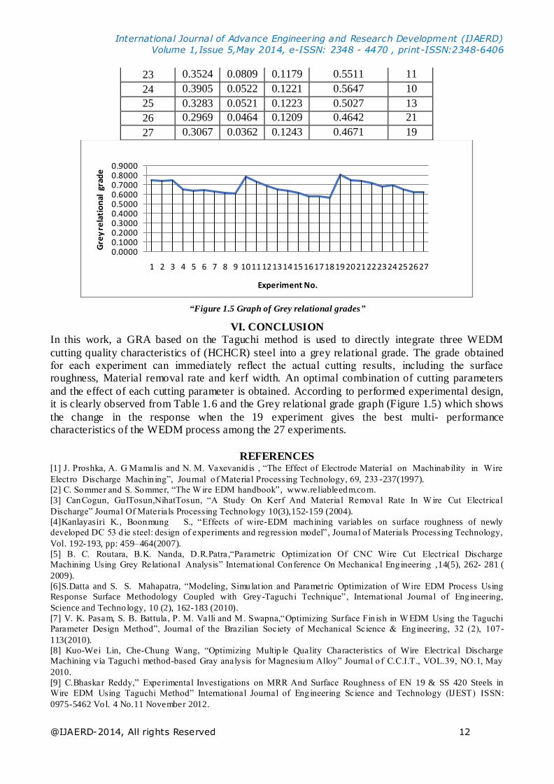
“Figure 1.5 Graph of Grey relational grades”
VI. CONCLUSION
In this work, a GRA based on the Taguchi method is used to directly integrate three WEDM
cutting quality characteristics of (HCHCR) steel into a grey relational grade. The grade obtained for each experiment can immediately reflect the actual cutting results, including the surface roughness, Material removal rate and kerf width. An optimal combination of cutting parameters
and the effect of each cutting parameter is obtained. According to performed experimental design, it is clearly observed from Table 1.6 and the Grey relational grade graph (Figure 1.5) which shows
the change in the response when the 19 experiment gives the best multi- performance characteristics of the WEDM process among the 27 experiments.
REFERENCES
[1] J. Proshka, A. G Mamalis and N. M. Vaxevanid is , “The Effect of Electrode Material on Machinab ility in Wire
Elect ro Discharge Machin ing”, Journal o f Material Processing Technology, 69, 233 -237(1997).
[2] C. Sommer and S. Sommer, “The W ire EDM handbook” , www.reliableedm.com.
[3] CanCogun, GulTosun,NihatTosun, “A Study On Kerf And Material Removal Rate In W ire Cut Electrical
Discharge” Journal Of Materials Processing Technology 10(3),152-159 (2004).
[4]Kanlayasiri K., Boonmung S., “Effects of wire-EDM machining variab les on surface roughness of newly
developed DC 53 d ie steel: design of experiments and regression model”, Journal of Materials Processing Technology,
Vol. 192-193, pp: 459–464(2007).
[5] B. C. Routara, B.K. Nanda, D.R.Patra,“Parametric Optimizat ion Of CNC Wire Cut Elect rical Discharge
Machining Using Grey Relational Analysis” Internat ional Conference On Mechanical Engineering ,14(5), 262- 281 (
2009).
[6]S.Datta and S. S. Mahapatra, “Modeling, Simulat ion and Parametric Optimization of Wire EDM Process Using
Response Surface Methodology Coupled with Grey-Taguchi Technique”, Internat ional Journal of Engineering,
Science and Technology, 10 (2), 162-183 (2010).
[7] V. K. Pasam, S. B. Battula, P. M. Valli and M. Swapna,“Optimizing Surface Fin ish in W EDM Using the Taguchi
Parameter Design Method”, Journal of the Brazilian Society of Mechanical Science & Engineering, 32 (2), 107-
113(2010).
[8] Kuo-Wei Lin, Che-Chung Wang, “Optimizing Multip le Quality Characteristics of Wire Electrical Discharge
Machining v ia Taguchi method-based Gray analysis for Magnesium Alloy” Journal o f C.C.I.T., VOL.39, NO.1, May
2010.
[9] C.Bhaskar Reddy,” Experimental Investigations on MRR And Surface Roughness of EN 19 & SS 420 Steels in
Wire EDM Using Taguchi Method” International Journal of Engineering Science and Technology (IJEST) ISSN:
0975-5462 Vol. 4 No.11 November 2012.
0.00000.10000.20000.30000.40000.50000.60000.70000.80000.9000
1 2 3 4 5 6 7 8 9 101112131415161718192021222324252627
Gre
y re
lati
on
al g
rad
e
Experiment No.