This document and trademark(s) contained herein are protected by law as indicated in a notice appearing later in this work. This electronic representation of RAND intellectual property is provided for non-commercial use only. Unauthorized posting of RAND PDFs to a non-RAND Web site is prohibited. RAND PDFs are protected under copyright law. Permission is required from RAND to reproduce, or reuse in another form, any of our research documents for commercial use. For information on reprint and linking permissions, please see RAND Permissions.

Limited Electronic Distribution Rights

This PDF document was made available from www.rand.org as a public

service of the RAND Corporation.

6Jump down to document

THE ARTS

CHILD POLICY

CIVIL JUSTICE

EDUCATION

ENERGY AND ENVIRONMENT

HEALTH AND HEALTH CARE

INTERNATIONAL AFFAIRS

NATIONAL SECURITY

POPULATION AND AGING

PUBLIC SAFETY

SCIENCE AND TECHNOLOGY

SUBSTANCE ABUSE

TERRORISM AND HOMELAND SECURITY

TRANSPORTATION ANDINFRASTRUCTURE

WORKFORCE AND WORKPLACE

The RAND Corporation is a nonprofit research organization providing objective analysis and effective solutions that address the challenges facing the public and private sectors around the world.

Visit RAND at www.rand.org

Explore Pardee RAND Graduate School

View document details

For More Information

Browse Books & Publications

Make a charitable contribution

Support RAND

This product is part of the Pardee RAND Graduate School (PRGS) dissertation series.

PRGS dissertations are produced by graduate fellows of the Pardee RAND Graduate

School, the world’s leading producer of Ph.D.’s in policy analysis. The dissertation has

been supervised, reviewed, and approved by the graduate fellow’s faculty committee.

PARDEE RAND GRADUATE SCHOOL

Selection, Wear, and TearThe Health of Hispanics and Hispanic Immigrants in the United States

Ricardo Basurto-Dávila

This document was submitted as a dissertation in May 2009 in partial fulfillment of the requirements of the doctoral degree in public policy analysis at the Pardee RAND Graduate School. The faculty committee that supervised and approved the dissertation consisted of Jose Escarce (Chair), Emma Aguila, and Krishna Kumar.

The RAND Corporation is a nonprofit research organization providing objective analysis and effective solutions that address the challenges facing the public and private sectors around the world. RAND’s publications do not necessarily reflect the opinions of its research clients and sponsors.

R® is a registered trademark.

All rights reserved. No part of this book may be reproduced in any form by any electronic or mechanical means (including photocopying, recording, or information storage and retrieval) without permission in writing from RAND.

Published 2009 by the RAND Corporation1776 Main Street, P.O. Box 2138, Santa Monica, CA 90407-2138

1200 South Hayes Street, Arlington, VA 22202-50504570 Fifth Avenue, Suite 600, Pittsburgh, PA 15213-2665

RAND URL: http://www.rand.orgTo order RAND documents or to obtain additional information, contact

Distribution Services: Telephone: (310) 451-7002; Fax: (310) 451-6915; Email: order@rand.org

The Pardee RAND Graduate School dissertation series reproduces dissertations that have been approved by the student’s dissertation committee.

 

iii 

 

ABSTRACT

The health of Hispanics in the United States is a complex issue that is still not well un-

derstood. Among the factors that complicate the study of Hispanic health are data arti-

facts and cultural differences that originate from different degrees of assimilation.

These problems may lead to biased estimations of the actual health profile of Hispanics

relative to other ethnic groups.

In this work, I seek to provide a better understanding of the issues surrounding the

health of Hispanics in general, and of Hispanic immigrants in particular. First, in

Chapter 2, I provide a brief review of the literature on Hispanic health, and I discuss

the hypotheses that have been proposed to explain three important results in that litera-

ture: (1) the apparent health advantage of Hispanics over other ethnic groups, despite a

relatively low socioeconomic status; (2) the decline in the health status of Hispanic im-

migrants as their length of residence in the United States increases; and (3) a weak or

even flat association between health and socioeconomic status among Hispanics.

In Chapter 3, I examine differences in health status between non-Hispanic Whites,

Mexican Americans, and Mexican immigrants. I propose an index of biological risk

composed by eight biomarkers that can be split into three subcomponents: inflamma-

tory, metabolic, and cardiovascular. The index gives more weight to biomarkers that

have stronger associations with mortality, and accounts for nonlinearities in those rela-

tionships. A separate set of analyses uses the Framingham risk score, a widely used indi-

cator of risk of coronary heart disease (CHD). In addition, I explore the application of

propensity score methods for the study of health disparities as an alternative to tradi-

tional regression analysis. Propensity score methods are more robust than regression to

systematic differences in the distribution of characteristics between the groups being

compared, and allow for simple assessment of the degree of overlap of those characteris-

tics.

To construct the health index, I use data from the Third National Health Examination

and Nutrition Survey (NHANES-III, 1988-1994) with linked mortality through 2000;

 

‐ iv ‐ 

the propensity score analyses use data from NHANES-III and the 1999-2004

NHANES. Results with allostatic load as the outcome indicate that there is no general

health advantage of Hispanics over Whites: Mexican Americans show higher (worse)

scores for the general index and all three subcomponents. Mexican immigrants, on the

other hand, have lower (better) inflammatory and cardiovascular scores, but higher

metabolic scores, than Whites. Conversely, results using Framingham risk as the out-

come suggest a general Mexican health advantage over Whites. Both US-born Mexicans

and Mexican immigrants have lower 10-year risk of CHD than Whites; and Mexican

immigrants enjoy an advantage in CHD risk over both Whites and US-born Mexicans.

The discrepancies between the analyses that use allostatic load and those that use the

Framingham score may be explained by the inclusion of smoking as a risk factor in the

Framingham score. The qualitative results do not change when regression analysis is

used, but the differences between the coefficients estimated using regression and pro-

pensity score methods are largest for the comparison of Mexican immigrants with

Whites, indicating that these two groups have the largest differences in observed covari-

ates and thus benefit the most from using propensity score methods.

In Chapter 4, I explore the Health-Age and Health-SES trajectories of Mexican immi-

grants using semiparametric methods. I assess the evidence supporting several of the

hypotheses discussed in Chapter 2. I find indirect evidence supporting the “healthy

migrant” hypothesis, which states that emigrants are positively selected in their health

status from the population of their countries of origin. My results are also consistent

with an apparent decline in immigrant health as the length of residence in the United

States increases, a common result in the literature. However, unlike several recent stud-

ies, I find that the Health-SES gradient is similar for Whites, recent immigrants, and

immigrants who have lived in the US for more than 15 years. Only immigrants who

have lived between 5 and 15 years in the US appear to have a weaker gradient. More-

over, I do not find support for the “acculturation hypothesis”, which states that the de-

cline in immigrant health with increased duration of residence is a result of assimilation

into US culture. In addition, my results suggest that this health decline is not likely to

be due to better average health among recent immigrant cohorts when compared to ear-

 

‐ v ‐ 

lier immigrant cohorts. Two hypotheses to explain the decline in immigrant health re-

main consistent with my results: (1) the “life-course” hypothesis, which states that the

deterioration of immigrant health status is a result of the cumulative negative effect of

the adversities associated with the process of migration, and (2) the “regression to the

mean” hypothesis, which maintains that immigrants self-select on health at the time of

migration, but over time their health converges to the average health levels in their

home countries. Finally, in Chapter 5, I summarize the main findings and I discuss the

implications of this work for future research and public policy.

 

vii 

ACKNOWLEDGEMENTS

 

I wish to thank my Committee for all their advice and willingness to help in every step of 

the dissertation process.  I cannot say enough about José’s role as a mentor; he was remark‐

able at guiding my efforts and not letting me become distracted by divergent ideas.  At every 

step of the way, his advice was just invaluable and I can confidently say that I could not have 

chosen a better Chair  for my Committee.   Emma always  found  time  to meet with me and 

discuss my ideas; she is a model for me to follow both for her dedication and for her profes‐

sionalism.   I am also thankful to Krishna, who was very understanding of the changes that 

moved this dissertation away from the topics we originally discussed, but was nonetheless 

always willing to help and discuss the new directions.  Brian Finch provided invaluable in‐

put  as  the  external  reader  and  has  always  been  supportive  of  my  development  as  a  re‐

searcher.    I  also  thank  Kip  and Mary  Ann  Hagopian,  who  supported my work  through  a 

dissertation  award  in  the  academic  year  2007‐2008.    Their  support  for  student  research 

through these awards has been invaluable to PRGS; I hope they are proud of the work they 

have contributed to produce. 

Getting a PhD is challenging, but it can be made so much easier by the people who sur‐

round you.  I have been very lucky in that respect.  Several people deserve special mention 

for  the  role  they  have  had  throughout my  life,  supporting my  professional  and  personal 

development:  Max  Garza,  Francisco  “Cesco”  Ciscomani,  David  Kendrick,  Wolfgang  Keller, 

Chloe Bird, Nicki Lurie, Lisa Meredith, Stephanie Taylor, and Lucrecia Santibáñez.   Others 

have offered me their friendship, advice, and sometimes just a smile whenever I needed it: 

every    “Chicote”  and  “Gansita” way back  in Zacatecas, Babur de  los  Santos, Marisela Gon‐

 

‐ viii ‐ 

zález,  Vero  Montes,  Lida  Sotres,  Paola  Méndez,  Lili  Rosas,  Alex  Solis,  Luis  Macías,  Javier 

Benito López, Juan Francisco “Pico” Fernández, Marco Oviedo, Miwa Hattori, Jason Cuomo, 

David  Howell,  Arkadipta  Ghosh,  Katya  Fonkych,  Leon  Cremonini,  Myong‐Hyun  Go,  Tom 

Lang, Mike Egner, Meena Fernandes, Khoa Truong, Ze Cong, Yang Lu, Seo Yeon Hong, and 

Ying Liu.   I am sure I failed to mention a few names, please do not be upset, next time you 

see me you will see the gratitude (and shame at my forgetfulness) in my face. 

Finally, I have no words to express my gratefulness to my family in Mexico.  My parents, 

who have always supported and  trusted  the decisions  I have made; and Chantal, who has 

remained strong and supportive despite the difficult times our family has gone through over 

the last couple of years.   Martha, you have been so patient,  I am so thankful and lucky for 

having you in my life.   

 

‐ ix ‐ 

TABLE OF CONTENTS

Chapter 1. Introduction and Research Questions ......................................................................1

1.1 Introduction .............................................................................................................................. 1

1.2 Research Goals ......................................................................................................................... 3

1.3 Organization.............................................................................................................................. 4

Chapter 2. Hispanic Health in the United States: A Review ....................................................7

2.1 Socioeconomic Profile of the Hispanic Population in the United States .......... 7

2.2 Hispanic Health........................................................................................................................ 9

2.3 Theories of Hispanic Health and the Hispanic Paradox........................................13

2.4 Limitations to Existing Data and Previous Analyses ..............................................15

Chapter 3. Health Differences Between US­Born Mexicans, Mexican  Immigrants and 

Non­Hispanic  Whites:  An  Analysis  of  the  Hispanic  Paradox  Using 

Propensity­Score Methods......................................................................................... 17

3.1 Introduction ............................................................................................................................17

3.1.1 Allostatic Load ............................................................................................................20

3.1.2 Framingham Risk Score ..........................................................................................22

3.2 Data and Measures ...............................................................................................................23

3.2.1 Data .................................................................................................................................23

3.2.2 Allostatic Load Measure..........................................................................................24

3.2.3 Framingham Risk Score (FRS) .............................................................................27

3.2.4 Imputation of Income Categories........................................................................29

3.3 Methodology of Analyses ...................................................................................................30

3.3.1 Doubly‐Robust Estimator: Propensity Score‐Weighted Regression....33

3.3.2 Model Building............................................................................................................37

3.3.3 Sensitivity Analyses..................................................................................................39

3.4 Results .......................................................................................................................................40

3.4.1 Construction of Allostatic Load Measure.........................................................40

3.4.2 Descriptive Statistics................................................................................................42

3.4.3 Common Support.......................................................................................................46

3.4.4 Matching Quality........................................................................................................47

3.4.5 Allostatic Load Model Results ..............................................................................52

 

‐ x ‐ 

3.4.6 Framingham Risk Score Results..........................................................................57

3.4.7 Sensitivity Analyses..................................................................................................65

3.5 Conclusion................................................................................................................................69

Chapter 4. Changes  in  Immigrant  Health  with  Length  of  Residence  in  the  United 

States: A Semiparametric Analysis.......................................................................... 73

4.1 Introduction ............................................................................................................................73

4.1.1 Hypotheses of Immigrant Health‐SES Gradient............................................73

4.1.2 Hypotheses of Immigrant Health Deterioration...........................................75

4.2 Data and Methodology ........................................................................................................78

4.2.1 Data .................................................................................................................................78

4.2.2 Methods .........................................................................................................................79

4.2.3 Estimation of AL‐Age and AL‐SES Relationships by Differencing .........82

4.2.4 Examining Hypotheses of Causes of  Immigrant Health Patterns Over 

Duration of Residence in the United States ...............................................................83

4.3 Results .......................................................................................................................................89

4.3.1  Changes  in  Allostatic  Load  With  Age  and  Income:  Whites  and 

Immigrants..............................................................................................................................89

4.3.2 Evidence For and Against Hypotheses of Changes in Immigrant Health 

Over Length of US Residence...........................................................................................96

4.4 Conclusion............................................................................................................................. 104

Chapter 5. Discussion ......................................................................................................................107

5.1 Main Findings ...................................................................................................................... 107

5.2 Future Research and Policy Implications................................................................. 109

 

 

‐ xi ‐ 

LIST OF TABLES

Table 1. US Foreign‐Born Population by Region of Birth, 2000‐2007............................................... 8

Table 2. Self‐Rated Health, by Ethnic Group...............................................................................................18

Table 3. Self‐Reported Chronic Disease Prevalence, by Ethnic Group ............................................19

Table 4. Framingham Scoring for 10‐year Risk of CHD (Men and Women)..................................28

Table 5. Estimated Coefficients from Survival Models for Allostatic Load Weights ..................43

Table 6. Descriptive Statistics of Original Sample (Averages/Proportions).................................44

Table 7.  Average Values of Eight Biomarkers, The Allostatic Load Index and its 

Subcomponents, and Framingham Risk Score; by Ethnic Group....................................45

Table 8. Propensity Score Minima/Maxima and Observations Removed from Sample...........47

Table 9. Descriptive Statistics of Propensity Score‐Weighted Samples—Estimated in the 

Common Support ................................................................................................................................49

Table 10. Ethnic Differences in Allostatic Load Scores ..........................................................................53

Table 11. Ethnic Differences in 10‐year Risk of CHD in Framingham Risk Score Models,  

Propensity‐Score Weighted Differences in Means................................................................58

Table 12. Rates of Smoking and Hypertension Treatment, Mexicans and Whites .....................61

Table 13. Ethnic Differences in Reduced Framingham Score, Propensity Score‐Weighted 

Differences in Means .........................................................................................................................62

Table 14.  Average Biomarker Values in NHANES Sample After Propensity Score‐Weighting, 

Non‐Hispanic Whites and Mexicans............................................................................................63

Table 15. Ethnic Differences in Reduced Allostatic Load Score, Propensity Score‐Weighted 

Differences in Means .........................................................................................................................64

Table 16. Summary of AL and FRS Propensity Score‐Weighted Estimates of Differences in 

Health Status Between Mexicans and Whites .........................................................................65

Table 17. Sensitivity Analyses: Coefficient Estimates under Alternative Models.......................67

Table 18. Sample Sizes of Mexican Immigrant and White Samples in Chapter 4 .......................79

Table 19.  Frequencies of Length of Time in the United States—Mexican Immigrants ...........84

Table 20.  Results of Partial Linear Model  Estimation—After Differencing out f(age) ...........89

Table 21. Results of Partial Linear Model Estimation‐‐After Differencing out g(pir) ...............90

Table 22. Specification Tests of Parametric Models—Non‐Hispanic Whites ...............................95

 

‐ xii ‐ 

 

xiii 

 

LIST OF FIGURES

Figure 1. Conceptual Model of Stress and Allostatic Load....................................................................21

Figure 2. Common Support Assessment: Distributions of Propensity Scores Before 

Adjustments ..........................................................................................................................................48

Figure 3. Covariate Balance Before and After Weighting with Propensity Scores .....................50

Figure 4. Boxplots of the Propensity Scores – Before and After PS‐Weighting ...........................51

Figure 5. Nonparametric Estimation of f(age) and g(pir)—Non‐Hispanic Whites and 

Mexican Immigrants ..........................................................................................................................93

Figure 6. Allostatic Load Age and SES Trajectories—Recent Immigrants vs. Non‐Hispanic 

Whites......................................................................................................................................................97

Figure 7. Allostatic Load‐Age and ‐SES Trajectories‐‐By Length of US Residence .....................99

Figure 8. Allostatic Load Age and SES Trajectories—NHANES‐III and 2001‐2004 NHANES

................................................................................................................................................................. 102

Figure 9. Allostatic Load Age and SES Trajectories—Spanish‐ vs. English‐Speaking 

Immigrants ......................................................................................................................................... 103

 

 

‐ xiv ‐ 

 

‐ 1 ‐ 

Chapter 1. Introduction and Research Questions

1.1 Introduction

It  is a well established  fact  that  individuals of higher socioeconomic status  live  longer 

and healthier lives.1  Since there are important differences in socioeconomic levels between 

racial and ethnic groups in the United States, it is not surprising to find that significant ra‐

cial/ethnic  disparities  exist  in  mortality  and  other  health  outcomes  (National  Center  for 

Health Statistics 2007; Keppel 2007; Cooper  et  al.  2000; Hahn and Eberhardt 1995; Vega 

and Amaro 1994).  However, socioeconomic differences between racial or ethnic groups are 

only part of the story regarding health disparities, as analyses of health disparities that ac‐

count  for  socioeconomic measures,  such as  income or education, do not explain  them en‐

tirely (LaVeist 2005; Williams and Collins 1995).  As a result, a large number of studies have 

been conducted in recent years trying to identify factors that may account for these dispari‐

ties in health outcomes, and policies that may be used to reduce them. 

In  particular,  many  questions  remain  unanswered  regarding  the  health  of  Hispanics. 

Several  studies  have  found  that  Hispanics  enjoy  better  health  and  lower  mortality  than 

other  racial/ethnic  groups,  including  non‐Hispanic  Whites.    This  phenomenon  has  com‐

monly  been  called  the Hispanic  Paradox  because Hispanics  have  low  socioeconomic  pro‐

files, more similar to those of non‐Hispanic Blacks than those of non‐Hispanic Whites, and 

thus we would expect them to have worse health outcomes than other ethnic groups with 

                                                             

1 Goldman (2001) provides a comprehensive review of the literature on social inequalities in health. 

 

‐ 2 ‐ 

higher  levels  of  socioeconomic  status  (SES).2    Over  the  last  two  decades,  several  studies 

have analyzed this phenomenon, using different outcome variables to compare the health of 

Hispanics with non‐Hispanics.  The results of these studies have provided mixed support for 

the existence of the paradox (see Chapter 2 for a review of the literature), but the general 

perception in the health literature is that Hispanics enjoy better health than expected given 

their socioeconomic status.  In addition, a few recent studies suggest an additional puzzling  

finding regarding Hispanic health: the association between SES and health may be weak or 

even positive  among Hispanics  (Goldman  et  al.  2006;  Turra  and Goldman 2007;  Zsembik 

and Fennell 2005).  

A distinctive characteristic of  the Hispanic population  in  the United States  is  the  large 

proportion of  immigrants among  its numbers.    In particular, Mexican  immigrants account 

for over 25 percent of all Hispanics in the country.  As is the case with Hispanics, available 

statistics indicate that Hispanic immigrants—Mexicans in particular—enjoy a better health 

status than other population groups in the United States.  Estimates from the 2006 National 

Health Interview Survey (NHIS) reflect a lower prevalence of cardiovascular disease, cancer, 

and asthma among Mexican immigrants than other immigrants and the native White popu‐

lation (CONAPO 2008).   

In  fact, Hispanic  immigration  could be an  important  factor  to  explain  the puzzling  re‐

sults described above  for  at  least  three  reasons:  (1) Mexican  immigrants  are  significantly 

younger than the rest of the US population, and thus should be less likely to suffer from sev‐

eral health conditions; (2) a  large number of  the Mexican‐born are recent  immigrants (30 

percent  arrived  in  2000  or  later)  and  are  thus  less  likely  to  correctly  respond  to  health‐

                                                             

2  From  hereafter,  for  simplicity,  I  will  refer  to  non‐Hispanic  Blacks  as  ‘Blacks’,  and  non‐Hispanic Whites as ‘Whites’. 

 

‐ 3 ‐ 

related  questions  in  population  surveys  due  to  their  lack  of  English  proficiency;  and  (3) 

perhaps the most important, health selection processes may be linked to immigration, such 

that  immigrants may be healthier  than  the population of  their  country of  origin,  and  less 

healthy immigrants may be more likely to return to their home country, leaving the healthi‐

est immigrant population in the United States.  These issues are discussed in more detail in 

Chapter 2.   

1.2 Research Goals

In this study, I contribute to the literature on health disparities—and Hispanic health in 

particular—by assessing the evidence supporting the existence of a Hispanic health advan‐

tage  over  non‐Hispanics,  and  exploring  the  patterns  of  immigrant  health  over  the  life‐

course.   My  first  contribution  is  the  construction  of  an  allostatic  load  index,  an  objective 

measure of health status not subject to biases due to group differences in culture or health 

literacy.    Although  allostatic  load  has  been  used  before  to  explore  the  Hispanic  Paradox 

(Crimmins et al. 2007), the measure I propose weighs its components accordingly to their 

independent associations with mortality, and accounts for non‐linearities in these associa‐

tions.    In  order  to  conduct  a more  thorough  assessment  of  the  existence  of  the  Hispanic 

Paradox, I also conduct analyses using the Framingham risk score, a well‐known measure of 

risk of coronary heart disease. 

My  second  contribution  is  the use of  semiparametric methods  for  the  study of  health 

disparities.  First, I use propensity score‐based methods to produce estimates of health dif‐

ferences between Hispanics and Whites that are not subject to potential biases tue to esti‐

mations  outside  the  region  of  common  support.    Second,  I  use  another  semiparametric 

method (differencing the partial linear model) to explore the age and SES associations with 

 

‐ 4 ‐ 

health among immigrants, and whether these associations vary with the length of residence 

in the United States.  

More specifically, I address the following research questions: 

1. Is there evidence supporting the existence of the Hispanic Paradox when comparing 

the health of non‐Hispanic Whites and individuals of Mexican ethnicity living in the 

United States? 

2. Does  the answer  to  the previous question change when  the Mexican  sample  is di‐

vided by country of birth (i.e., Mexico and the United States)? 

3. Are there differences between Mexican immigrants and non‐Hispanic Whites in the 

associations between age and socioeconomic status with health? 

4. What factors could explain the patterns found in question 3? In particular: 

a. Is there evidence of immigrant health selection? 

b. Do the health‐age and health‐SES patterns change with immigrants’ length of 

residence in the United States? 

c. Are there health differences between immigrant cohorts? 

d. Are  there health differences between  immigrants with different degrees of 

acculturation? 

1.3 Organization

This dissertation is organized as follows: In Chapter 2, I briefly summarize the literature 

on Hispanic Health, in particular that on the Hispanic Paradox, and I discuss the hypothesis 

that can potentially explain some of the results found by previous studies that are relevant 

for my work on this dissertation. In Chapter 3, I examine the existence of the Hispanic Para‐

dox using propensity score methods and two summary indicators of health status: allostatic 

 

‐ 5 ‐ 

load and Framingham risk  scores.    In  this  chapter,  I  first discuss  the  concept of allostatic 

load as a measure of biological risk and the use of Framingham scores as measures of risk of 

coronary heart  disease.   Next,  I  describe  the data  from  the National Health  and Nutrition 

Examination Survey and  I explain  the procedure  I  follow  to create a measure of allostatic 

load that accounts  for  its components’ relationships with mortality and for non‐linearities 

in those relationships.   Later  in the same chapter,  I discuss propensity score methods and 

their advantages over commonly used regression, focusing on the doubly robust method of 

propensity‐score weighted regression, which I use to estimate allostatic load and Framing‐

ham risk differences between Hispanics and non‐Hispanic Whites.    I present the results of 

these estimations and conclude this chapter with a discussion of policy and future research 

implications.   In Chapter 4, I explore the health­age and health­SES trajectories of Mexican 

immigrants  using  semiparametric methods.    I  assess  the  evidence  supporting  several  hy‐

potheses regarding the health selectivity of migration and the changes in health over immi‐

grants’ lifetime.  Finally, in Chapter 5, I summarize the results and discuss the implications 

for future research and policy. 

 

‐ 7 ‐ 

Chapter 2. Hispanic Health in the United States: A Review

In  this  chapter,  I  describe  the  socioeconomic  and  demographic  characteristics  of  the 

Hispanic population  in the United States, and discuss the findings of  the  literature on His‐

panic health.   Although Hispanics are not a homogenous population—there are significant 

health and socioeconomic differences between Hispanic subgroups—, I focus on Hispanics 

in general and Mexicans in particular.  The main reason for this is that my empirical analy‐

ses in the following chapters use data only on Mexican Americans and Mexican immigrants.  

The review of the literature is in no way complete.  Nonetheless, it presents a representative 

set of the studies most relevant to the issues addressed in this dissertation. 

2.1 Socioeconomic Profile of the Hispanic Population in the United States3

The Hispanic population in the United States has grown at a notably fast rate over the 

last three decades and they are now the largest minority group in the country.  Figures from 

the 2000 census placed Hispanics at around 35 million people, a 58 percent increase since 

1990.  Estimates from the American Community Survey indicate that this growth has hardly 

slowed down: Hispanics  increased  their numbers by 29 percent between 2000 and 2007, 

for an estimated Hispanic population of 45 million in 2007, the last year for which estimates 

are  available.   Notably,  over  the 21st  century Hispanics have accounted  for 50 percent of 

total population growth in the United States (Fry 2008). 

                                                             

3 Unless otherwise noted, numbers cited in Section 2.1 were obtained from the Pew Hispanic Center’s Statistical  Portrait  of  Hispanics  in  the  United  States,  2007,  online  at  http://pewhispanic.org/factsheets/factsheet.php?FactsheetID=46.  

 

‐ 8 ‐ 

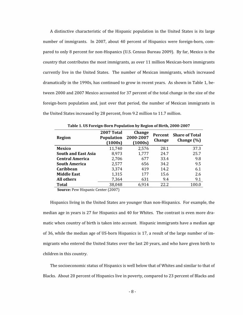
A distinctive  characteristic  of  the Hispanic population  in  the United  States  is  its  large 

number  of  immigrants.    In  2007,  about  40  percent  of  Hispanics were  foreign‐born,  com‐

pared to only 8 percent for non‐Hispanics (U.S. Census Bureau 2009).  By far, Mexico is the 

country that contributes the most immigrants, as over 11 million Mexican‐born immigrants 

currently  live  in  the United  States.    The number  of Mexican  immigrants, which  increased 

dramatically in the 1990s, has continued to grow in recent years.  As shown in Table 1, be‐

tween 2000 and 2007 Mexico accounted for 37 percent of the total change in the size of the 

foreign‐born population  and,  just  over  that period,  the number  of Mexican  immigrants  in 

the United States increased by 28 percent, from 9.2 million to 11.7 million.   

Table 1. US Foreign­Born Population by Region of Birth, 2000­2007 

Region 2007 Total  Population  

(1000s) 

Change 2000­2007 

(1000s) 

Percent  Change 

Share of Total  Change (%) 

Mexico  11,740 2,576 28.1 37.3South and East Asia  8,973 1,777 24.7 25.7Central America  2,706 677 33.4 9.8South America  2,577 656 34.2 9.5Caribbean  3,374 419 14.2 6.1Middle East  1,315 177 15.6 2.6All others  7,364 631 9.4 9.1Total  38,048 6,914 22.2 100.0

    Source: Pew Hispanic Center (2007) 

 

Hispanics living in the United States are younger than non‐Hispanics.  For example, the 

median age in years is 27 for Hispanics and 40 for Whites.  The contrast is even more dra‐

matic when country of birth is taken into account.  Hispanic immigrants have a median age 

of 36, while the median age of US‐born Hispanics is 17, a result of the large number of im‐

migrants who entered the United States over the last 20 years, and who have given birth to 

children in this country. 

The socioeconomic status of Hispanics is well below that of Whites and similar to that of 

Blacks.  About 20 percent of Hispanics live in poverty, compared to 23 percent of Blacks and 

 

‐ 9 ‐ 

9 percent of Whites.  Hispanic median household income in 2007 was $40,500, compared to 

$54,700 for Whites, and $33,800 for Blacks.  In terms of educational attainment, 24 percent 

of Hispanics of age 25 and older have an education of  less  than 9th grade, compared to 3 

percent of Whites and 6 percent of Blacks.  Accordingly, only 13 percent of Hispanics have a 

college degree, compared with 31 percent of Whites and 17 percent of Blacks.  In education, 

there  are  important  differences  between  US‐born  and  foreign‐born  Hispanics,  as  only  9 

percent of native Hispanics have an education less than 9th grade, but the figure is 34 per‐

cent for Hispanic immigrants. 

2.2 Hispanic Health

The health of Hispanics began to receive attention in the public health literature only in 

the  last  two  decades.  Before,  the  common  assumption  was  that  Hispanic  health  profiles 

were  similar  to  those  of  other minorities with  similar  socioeconomic  conditions,  such  as 

African Americans (Vega and Amaro 1994).  However, an increasing number of studies indi‐

cate  that  the  issues  surrounding  Hispanic  health  are  significantly  different  from  those  of 

other  minority  groups.    A  topic  that  has  recently  dominated  the  literature  on  Hispanic 

health is the so‐called “Hispanic Paradox”, the apparent health advantage of Hispanics over 

other ethnic groups, despite their lower socioeconomic profile.  More recently, a handful of 

studies have  identified a  “second paradox”:  the association between socioeconomic status 

and health appears to be weaker among Hispanics than among other groups.  Below, I dis‐

cuss the main findings and yet‐to‐be‐answered questions related to Hispanic health. 

Markides and Coreil (1986) were the first to refer to the health status of Hispanics in the 

United  States  as  an  “epidemiological  paradox”.  Conducting  a  review  of  previous  studies, 

they concluded that the health status of Hispanics in Southwestern United States was closer 

to the health status of Whites than to that of African Americans.  Among the health indica‐

 

‐ 10 ‐ 

tors  where  the  authors  found  this  health  similarity  between  Hispanics  and Whites  were 

infant mortality, life expectancy, mortality from cardiovascular diseases, cancer, and meas‐

ures of  functional health.   Markides and Coreil called this phenomenon a paradox because 

Hispanics have a risk profile more similar to that of Blacks than that of Whites in terms of 

their socioeconomic status.   

Since Markides and Coreil’s article, a number of studies have explored the existence of 

the Hispanic Paradox.  Franzini, Ribble, and Keddie (2001) conducted a comprehensive re‐

view of the literature on Hispanic health between the years 1963 and 1999.   Their search 

identified nearly 200 relevant articles, of which they chose 89 to summarize in their review.  

One interesting finding of their review is that the Hispanic Paradox appears to be a recent 

phenomenon, since mortality studies conducted in the 1950s and through the 1970s gener‐

ally found higher mortality rates for Hispanics—identified at the time by their Spanish sur‐

names—than for Whites.    It was not until data from the 1980 US census became available 

that mortality rates were found to be lower for Hispanics than for Whites at certain ages. 

Several articles reviewed by Franzini, Ribble, and Keddie studied the mortality of His‐

panics.   Among them, Liao et al. (1998) used 1986‐1990 data from the National Health In‐

terview Survey, linked to the National Death Index (NDI), to assess the mortality patterns of 

the adult Hispanic population in the US and compare it to mortality patterns of Whites and 

Blacks.   They found that Hispanic males have higher mortality rates than Whites at ages 18 

to 44 (rate ratio equal to 1.33), similar mortality rates at ages 45 to 64 (RR=0.92), and lower 

mortality rates at ages equal to or over 65 (RR=0.76).   For females, the mortality ratios at 

the same age categories were 1.22, 0.75, and 0.70, respectively, where only  the  latter  two 

were  statistically  significant.    Blacks  had  consistently  higher  mortality  rates  than  both 

Whites and Hispanics.  Similar results are found by Sorlie et al. (1993), who used data from 

the Current Population Survey matched to the NDI, and found that Hispanics had lower all‐

 

‐ 11 ‐ 

cause mortality rates  than non‐Hispanics, as well as  lower mortality  from cancer and car‐

diovascular disease; on  the other hand, Hispanics had higher mortality  from diabetes and 

homicide.  

Other studies have used self‐reports of health status or health conditions.   Drawing on 

1989‐2004  data  from  the  National  Health  Interview  Survey,  Cho  et  al.  (2004)  examined 

Hispanic  subgroup  differences  in  three  measures  of  health  status:  self‐reported  overall 

health, daily activity limitations, and number of days spent in bed due to illness.  They found 

that Puerto Ricans exhibit the worst health profiles among Blacks, Whites, and all Hispanic 

subgroups.    Individuals  of  Central/South American  and Mexican  origin  are  found  to  have 

lower risk of activity limitations and number of bed days than Whites.  Finally, all Hispanic 

subgroups were more likely to report fair or poor health status than Whites. 

A Hispanic health advantage has been found not only for adults, but also in infant mor‐

tality and birthweight.   Kleinman (1990) used 1983 and 1984 data on linked birth and in‐

fant‐death  records.   He  finds  that  “despite  a high  rate of poverty  and  low use of prenatal 

care,  Mexicans  have  approximately  the  same  [infant  mortality  rate]  as  non‐Hispanic 

whites.” Regarding the heterogeneity of infant health outcomes among Hispanics, Becerra et 

al. (1991) and Albrecht et al. (1996) obtain similar findings: Puerto Ricans are the least ad‐

vantaged group among Hispanics, while Cubans are the most advantaged.  The first of these 

two studies also found that Mexicans had an infant mortality risk similar to that of Whites.  

In a more recent study, Luke et al.  (2005)  found that Hispanic women had  lower propor‐

tions of  low birth weight and preterm births—and higher average birth weight and gesta‐

tion periods—than White and Black women. 

On  the  other  hand,  some  studies  have  found  no Hispanic  health  advantage,  and  even 

disadvantages in some health outcomes.  For example, the results of several studies indicate 

a Hispanic disadvantage  in  the  incidence of diabetes  (Hamman et al. 1989; Marshall et al. 

 

‐ 12 ‐ 

1993), metabolic syndrome (Park et al. 2003), and obesity (Abraido‐Lanza, Chao, and Florez 

2005).  Mitchell et al. (1992) try to determine whether Mexican Americans are more resis‐

tant than Whites to the cardiovascular effects of diabetes.   They formulate this hypothesis 

based on  the  fact  that Mexican Americans have  a high prevalence of  diabetes when  com‐

pared to Whites, but experience lower cardiovascular mortality.  They find that the associa‐

tions of diabetes with myocardial infarction and coronary heart disease (CHD) risk factors 

are at least as strong, if not stronger, in Mexican Americans as in Whites.  Interestingly, they 

still conclude that Mexican ethnicity confers protective effects against CHD, but this protec‐

tion may be obscured by their high prevalence of diabetes. 

Markides and Eschbach (2005) review recent research on the existence of the Hispanic 

Paradox.  They conclude that most evidence indicates the existence of the Paradox.  Studies 

that used datasets with better data quality—such as Medicare data linked to records from 

the  Social  Security Administration—find  a  significantly  lower mortality  advantage  of His‐

panics over Whites than studies that used vital statistics or linkages to the National Death 

Index, which indicates that poor data quality may indeed bias the results towards a larger 

Hispanic mortality advantage.   Nevertheless, they conclude that the evidence supports the 

existence of the Paradox, at least for individuals of Mexican origin. 

An additional puzzling result regarding Hispanic health has been identified by a few re‐

cent studies:  the almost universally accepted positive association between SES and health 

may be weak or non‐existing among Hispanics  in  the US.   This weak association between 

SES  and  health  has  been  found  for mortality  and  several  variables  related  to  health  and 

health  behaviors  (Goldman  et  al.  2006;  Turra  and  Goldman  2007;  Kimbro  et  al.  2008; 

Acevedo‐Garcia, Soobader, and Berkman 2007).  In fact, at least one study found that worse 

health  is  associated with higher  SES  levels  among Mexicans  (Zsembik  and Fennell  2005).  

That such a  result has escaped  the attention of most of  the  literature  is puzzling by  itself.  

 

‐ 13 ‐ 

Turra and Goldman (2007) suggest that this may be because some scholars have focused on 

racial/ethnic health differences while others have been mainly interested in the association 

between SES and health, with both groups assuming a constant overall SES‐health relation‐

ship,  thus  paying  little  attention  to  possible  variations  in  the  SES‐health  gradient  across 

racial/ethnic groups.    In  fact,  it  is  likely  that  the  two phenomena discussed  in  this section 

are  interconnected.    Several of  the processes  that have been proposed  to explain  the His‐

panic Paradox—described in more detail below—might also result in weak Health­SES gra‐

dients. 

2.3 Theories of Hispanic Health and the Hispanic Paradox

Three major  hypotheses  have  been proposed  to  explain  the Hispanic  Paradox,  two of 

them associated with immigration.  First, several authors have argued that the Paradox is a 

result of Hispanic culture, which promotes better health behaviors and stronger social sup‐

port among Hispanics than among non‐Hispanics (Markides and Coreil 1986; Mitchell et al. 

1990; Vega et al. 1991).  Hispanics are less likely than non‐Hispanics to smoke tobacco and 

drink  alcohol  (National  Center  for  Health  Statistics  2007),  two  important  risk  factors  for 

poor  health  outcomes.    Moreover,  it  has  been  posited  that  social  principles  in  Hispanic 

countries result in stronger social support that positively affects health (Kana'Iaupuni et al. 

2005).    If  these  behaviors  and  social  principles  are  passed  across  generations,  Hispanics 

that maintain  cultural  ties  to  their  countries  of  origin—or  of  their  ancestors—will  enjoy 

better health and lower risk of mortality. 

The second hypothesis to explain the Hispanic Paradox is usually called the “healthy mi­

grant”  theory (Abraido‐Lanza et al. 1999; Jasso et al. 2004).   Under this hypothesis,  immi‐

grants  are  assumed  to  be  a  non‐representative  sample  from  the  population  of  their 

countries of origin.  Because of the difficulties and risks associated with the process of emi‐

 

‐ 14 ‐ 

gration, individuals who attempt and succeed in migrating to more developed countries are 

likely to be positively selected in a number of traits, including health status.  Although this 

hypothesis directly explains only better‐than‐expected health among immigrants, a possible 

explanation for a health advantage of Hispanics in general over other ethnic groups is that 

the US‐born offspring of recent migrants inherit this good health from their parents’ genes.  

The latter supposition is not often mentioned in the literature, but it is an implicit assump‐

tion in studies that conclude that a health advantage exists for all Hispanics, and that it is a 

result of  the healthy migrant effect.   The healthy migrant hypothesis  is, perhaps,  the most 

commonly accepted assumption in the Hispanic health literature, even though the evidence 

for it is not very clear (Rubalcava et al. 2008). 

Finally, a  third potential explanation  for  the Hispanic Paradox  is  the “salmon bias” hy‐

pothesis, which states that certain immigrants may be more likely to return to their coun‐

tries of origin,  such as  the unemployed,  retired, or  those who are  ill  (Abraido‐Lanza et al. 

1999).  The latter group gives the hypothesis its name, as some of these migrants would be 

returning to their home country only to die.  If returning Hispanic migrants are more likely 

to  be  in worse  health  than  those who  remain  in  the United  States, measures  of Hispanic 

morbidity and mortality collected in the United States will be biased downwards, indicating 

a spurious health advantage of Hispanics over other ethnic groups.  Although some authors 

have  argued  that  the  salmon  bias  is  an  important  explanation  of  the  Hispanic  Paradox 

(Palloni and Arias 2004), recent evidence indicates that its effect is of too small a magnitude 

to fully explain it (Turra and Elo 2008). 

In addition to the hypotheses that have been suggested to explain the Hispanic Paradox, 

a common premise in the Hispanic health literature is that the health of Hispanics deterio‐

rates  as  they  assimilate  into  US  culture  and  their  health  behaviors  worsen  (Antecol  and 

Bedard 2006).  The acculturation hypothesis originates from the apparent reduction in the 

 

‐ 15 ‐ 

immigrant health advantage over time, which would result  in a convergence of  immigrant 

health  to  that  of  the  native  non‐Hispanic  population.    Although  acculturation  is  the most 

commonly proposed explanation  for  this phenomenon, other  factors may produce  similar 

results, such as recent immigrant cohorts that are healthier than earlier cohorts, a reversion 

of  immigrant health to the average health  levels  in their countries, or the accumulation of 

adverse  life  events  unrelated  to  acculturation  (Stephen  et  al.  1994;  Jasso  et  al.  2004; 

Hertzman 2004). 

2.4 Limitations to Existing Data and Previous Analyses

An important issue in the study of Hispanic health is the lack of quality and availability 

of data that allows for an adequate assessment of the health of Hispanics relative to other 

ethnic groups, and of  its changes over time.   One and a half decades ago, Vega and Amaro 

(1994) described the limitations of the data systems available at the time: 

“(a) [T]hey do not collect appropriate and accurate data on Hispanic ethnicity; (b) they 

do not sample sufficiently large numbers of Hispanics; and (c) they fail to tabulate and 

report data separately  for Hispanics.   Moreover,  the Council of Scientific Affairs of  the 

American Medical  Association  concluded,  ‘Accurate  estimates  of  Hispanic  death  rates 

are  impossible  to determine because, until 1988,  the national model death certificates 

did not contain Hispanic identifiers’.” 

Ten years later, Palloni and Arias (2004) still found problems with the quality of data‐

sets  of  Hispanic mortality  and morbidity, which  included  the  underreporting  of  Hispanic 

ethnicity,  the misreporting  of  ages,  and  the mismatching  of  death  records.    Each  of  these 

data artifacts  identified by Palloni and Arias may  lead  to spurious estimates of a Hispanic 

health advantage.  In fact, Smith and Bradshaw (2006) argue that the under‐identification of 

Hispanic ethnicity in death statistics accounts for the differences in life expectancy between 

 

‐ 16 ‐ 

Hispanics and non‐Hispanic Whites, and thus they conclude that “there is no Hispanic Para‐

dox.”   However,  studies  that have used better‐quality data, have  found mortality rates  for 

Hispanics  that,  although  higher  than  those  estimated  from  vital  statistics,  are  still  lower 

than those of non‐Hispanics (Elo et al. 2004; Hummer, Benjamins, and Rogers 2004).  

 

‐ 17 ‐ 

Chapter 3. Health Differences Between US-Born Mexicans, Mexican Immi-grants and Non-Hispanic Whites: An Analysis of the Hispanic Paradox Using Propensity-Score Methods

3.1 Introduction

The evidence discussed in Chapter 2 indicates the existence of a Hispanic health advan‐

tage over other ethnic groups.  However, in addition to the data problems related to assess‐

ing the mortality of Hispanics, discussed in section 2.4, there are other potential biases that 

may arise as a result of the use of self‐assessments of health status and self‐reports of health 

conditions.  This is a particularly important issue for the study of Hispanic health because of 

the large number of Hispanics who are either immigrants or offspring of recent immigrants, 

which may result in low degrees of assimilation into US culture and its institutional setting 

for an important number of Hispanics.  Commonly used self‐reported health indicators may 

produce biased results when they are used to compare ethnic groups with different levels of 

acculturation, such as Hispanic immigrants and US‐born Whites (Finch et al. 2002).   

An  illustration  is  probably  useful  to  explain  the  last  point.    Table  2  compares  self‐

reported health by racial/ethnic groups  in the 1988‐1994 and 1999‐2004 National Health 

and  Nutrition  Examination  Survey  (NHANES).    Whites  and  Blacks  seem  to  enjoy  better 

health  than Mexicans  in general,  as  they have higher proportions of  individuals  reporting 

“excellent” or “very good” health (57 percent  for Whites, 41 percent  for Blacks, 33 percent 

for Mexicans) and lower proportions reporting “fair” or “poor” health (14, 22, and 29 per‐

cent, respectively).   Moreover, when Mexicans are divided by country of birth, immigrants 

 

  ‐ 18 ‐ 

appear  to be  the  least healthy ethnic group among those displayed  in  the table, while US‐

born Mexicans display self‐rated health patterns similar to those reported by Blacks.   

Table 2. Self­Rated Health, by Ethnic Group 

  Excellent  Very Good  Good  Fair  Poor Whites  23% 34% 30% 11%  3%Blacks  18% 23% 36% 18%  4%Mexicans (all)  14% 19% 38% 25%  4%   Mexicans:       Immigrants  12% 14% 40% 29%  4%    US‐Born   17% 26% 35% 18%  4%

Source: NHANES‐III and NHANES 1999‐2004 

 

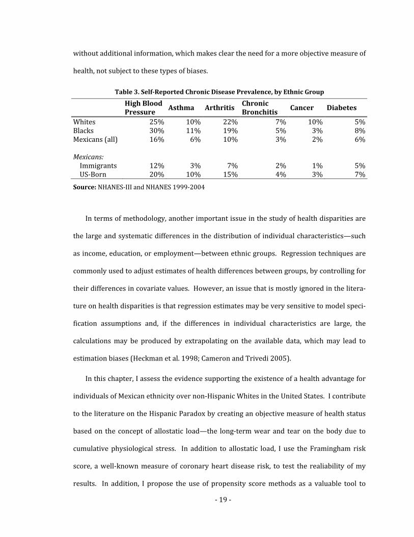
On the other hand, the picture becomes significantly less clear when the prevalence of 

chronic diseases (shown in Table 3) is examined by racial/ethnic group.  In this case, Mexi‐

cans  report  the  lowest  incidence of  five of  six  chronic  conditions, diabetes being  the only 

one where  they  report  slightly higher prevalence  than Whites.    Furthermore, when Mexi‐

cans  are  examined  by  country  of  birth,  immigrants  are  the  ethnic  group with  the  lowest 

disease prevalence, by far and across the board.  Since immigrants are on average younger 

than the native US population, the differences observed in Table 3 could be explained sim‐

ply because younger people are less likely to suffer from chronic conditions.  However, Jasso 

et al (2004) examined similar tabulations, stratified by age groups, using data from the Na‐

tional  Health  Interview  Survey  and  found  similar  patterns  of  self‐rated  health  and  self‐

reported chronic conditions.  As they discuss, these figures could be interpreted as indicat‐

ing  that  immigrants  (or  Mexicans  in  general)  may  subjectively  self‐report  themselves  as 

having worse health  than  they actually have.   An alternative explanation  is  that Mexicans 

indeed have worse health than Whites and Blacks but under‐report their suffering of spe‐

cific chronic diseases, either because of cultural differences or lack of access to medical di‐

agnoses.    Determining  which  of  these  conjectures,  if  either,  is  correct  cannot  be  done 

 

  ‐ 19 ‐ 

without additional information, which makes clear the need for a more objective measure of 

health, not subject to these types of biases.  

Table 3. Self­Reported Chronic Disease Prevalence, by Ethnic Group 

 High Blood Pressure 

Asthma  Arthritis Chronic Bronchitis 

Cancer  Diabetes 

Whites  25%  10% 22% 7% 10%  5%Blacks  30%  11% 19% 5% 3%  8%Mexicans (all)  16%  6% 10% 3% 2%  6%     Mexicans:         Immigrants  12%  3% 7% 2% 1%  5%    US‐Born   20%  10% 15% 4% 3%  7%

Source: NHANES‐III and NHANES 1999‐2004 

 

In terms of methodology, another important issue in the study of health disparities are 

the large and systematic differences  in the distribution of  individual characteristics—such 

as income, education, or employment—between ethnic groups.  Regression techniques are 

commonly used to adjust estimates of health differences between groups, by controlling for 

their differences in covariate values.  However, an issue that is mostly ignored in the litera‐

ture on health disparities is that regression estimates may be very sensitive to model speci‐

fication  assumptions  and,  if  the  differences  in  individual  characteristics  are  large,  the 

calculations may  be  produced  by  extrapolating  on  the  available  data,  which may  lead  to 

estimation biases (Heckman et al. 1998; Cameron and Trivedi 2005). 

In this chapter, I assess the evidence supporting the existence of a health advantage for 

individuals of Mexican ethnicity over non‐Hispanic Whites in the United States.  I contribute 

to the literature on the Hispanic Paradox by creating an objective measure of health status 

based on  the  concept of  allostatic  load—the  long‐term wear and  tear on  the body due  to 

cumulative  physiological  stress.    In  addition  to  allostatic  load,  I  use  the  Framingham  risk 

score,  a well‐known measure of  coronary heart disease  risk,  to  test  the  realiability of my 

results.    In  addition,  I  propose  the  use  of  propensity  score methods  as  a  valuable  tool  to 

 

  ‐ 20 ‐ 

study health disparities because they allow the researcher to assess the  lack of overlap  in 

the characteristics of the groups being compared, an issue often overlooked in these studies.  

Below, I discuss the concept of allostatic load and the Framingham risk score.  In section 

3.2,  I describe the data from the National Health Nutrition and Examination Survey,  intro‐

duce the measure of allostatic  load, and describe the construction of the Framingham risk 

score.  Section 3.3 discusses propensity score methods, and the doubly‐robust estimator: a 

consistent  estimator  of  differences  in  outcomes  between  groups,  even  in  the  presence  of 

misspecifications in one of the two steps that compose it.  In section 3.4, I discuss the results 

of the allostatic load measure construction, the assessment of overlap in the distribution of 

covariates between non‐Hispanic Whites and Mexicans,  and  the estimations of health dif‐

ferences between these two groups using allostatic load and the Framingham score.  Section 

3.5 concludes the chapter with a discussion of the results and their implications. 

3.1.1 Allostatic Load

Stressful  experiences—major  life  events,  noise,  hunger,  isolation,  temperature  ex‐

tremes, trauma, abuse, or infections—trigger physiological responses in an attempt to pro‐

tect the body.  Among others, the nervous, cardiovascular, metabolic, and immune systems 

activate biological mechanisms that seek to achieve stability  through physiological adjust‐

ments.   This ability of the human body to achieve stability through change is known as al­

lostasis (Sterling and Eyer 1988).  

Figure 1,  adapted  from McEwen  (1998), depicts  a  conceptual model of  the process of 

adaptation  to  stressful  stimuli.   An  individual’s  ability  to adapt  to  continuous or  repeated 

stress depends on several  factors, which  include genetics, physical condition, and idiosyn‐

crasy.  Under normal circumstances, the physiological response to stress is sustained for an 

interval long enough to appropriately respond to the stressor and is then turned off.  How‐

 

  ‐ 21 ‐ 

ever, different situations may arise in which either frequent stress or insufficient adaptation 

result  in  physiological  damage  (McEwen  and Wingfield  2003).    This  long‐term wear  and 

tear, experienced by the body as it struggles to achieve stability in stressful situations, has 

been called allostatic load (McEwen and Stellar 1993; McEwen and Seeman 1999).   

Figure 1. Conceptual Model of Stress and Allostatic Load 

PerceivedStress

PhysiologicResponse

EnvironmentalStressors

Major LifeEvents

Trauma,Abuse

Individual Differences(genetics, physical

condition, experience)

Behavioral Responses(timid/aggressive,health behaviors)

Allostasis Adaptation

AllostaticLoad

PerceivedStress

PhysiologicResponse

EnvironmentalStressors

Major LifeEvents

Trauma,Abuse

Individual Differences(genetics, physical

condition, experience)

Behavioral Responses(timid/aggressive,health behaviors)

Allostasis Adaptation

AllostaticLoad

 

The concept of allostatic load has been operationalized in recent studies through sum‐

mary indices of several biomarkers.  For example, Seeman et al (1997) developed a measure 

of allostatic load using 10 parameters: systolic and diastolic blood pressure, waist‐hip ratio, 

serum high‐density lipoprotein (HDL) and total cholesterol levels, plasma levels of glycosy‐

lated hemoglobin, serum dehydroepiandrosterone sulfate (DHEA‐S), 12‐hour urinary corti‐

sol  excretion,  and 12‐hour urinary norepinephrine  and  epinephrine  excretion  levels.    For 

each of  these parameters,  individuals were classified  into quartiles based on  the sample’s 

 

  ‐ 22 ‐ 

distribution of  their  values,  and  the  allostatic  load  score  for  each  individual  is  created by 

adding the number of parameters for which the subject fell into the highest‐risk quartile.   

Allostatic load has been shown to be a consistent predictor of mortality, cardiovascular 

disease, decline in physical functioning, and decline in cognitive functioning (Seeman et al. 

1997; Karlamangla et al. 2002; Seeman et al. 2001).  Since allostatic load is a result of indi‐

vidual exposure to stress, and exposure is a function of several factors, including social and 

economic conditions, it has also been proposed as a likely mediator between socioeconomic 

status and health outcomes.  Consistently with this idea, several studies have found signifi‐

cant associations between allostatic  load and several measures of socioeconomic and psy‐

chosocial  status  such  as  education,  hostility,  disadvantaged  environments,  and  poverty 

(Kubzansky, Kawachi, and Sparrow 1999; Evans 2003; Johnston‐Brooks et al. 1998).  

3.1.2 Framingham Risk Score

The Framingham risk score (FRS) is a widely used measure to predict the risk of coro‐

nary heart disease (CHD) in the general population.  This score was derived from the results 

of the Framingham Heart Study (Anderson et al. 1991; Wilson et al. 1998), a series of stud‐

ies of population‐based samples with  follow‐up  intervals of several years  that allowed re‐

searchers to derive scoring algorithms to estimate the risk of CHD.  The Framingham score 

includes  risk  factors  such as age,  gender,  smoking, blood pressure,  and  cholesterol  levels.  

The application of a scoring formula that accounts for different combinations of these fac‐

tors results in a total score that can be used to estimate the 10‐year risk of CHD for a given 

individual.   The Framingham scoring system has been validated for individuals of ages 20‐

79 (NCEP 2001).   Other studies have shown that the risk factors in the Framingham score 

do less well in predicting the risk of CHD for individuals of age 85 and older (de Ruijter et al. 

2009). 

 

  ‐ 23 ‐ 

3.2 Data and Measures

3.2.1 Data

I use data from the 1988‐1994 and 1999‐2004 releases of the National Health and Nu‐

trition  Examination  Survey  (NHANES‐III  and  continuous  NHANES),  a  series  of  cross‐sec‐

tions  representative  of  the  non‐institutionalized  US  population  (NCHS  2005).    NHANES 

includes  individual  data  on demographic  and  socioeconomic  characteristics,  diet, medical 

examinations, physical measurements, and  laboratory tests.   Mexican Americans and Afri‐

can Americans were over‐sampled, so each of these groups represents around one fourth of 

each  cross‐section;  the Mexican‐born  account  for  50‐60  percent  of  the Mexican‐ethnicity 

samples.  In addition, I use the NHANES‐III National Death Index (NDI) linkage to construct 

the allostatic load measure; the NDI linkage provides mortality follow‐up information from 

the date of survey participation (1988‐1994) through December 31, 2000 for all NHANES‐

III adult participants (ages 17 and older).4  

I restrict the data to individuals 20 years of age and older who attended the mobile ex‐

amination  centers  where  the  physical  exams  and  laboratory  samples  were  collected.    In 

addition,  I  remove women who  reported  to  be  pregnant  or were  found  pregnant  by  the 

laboratory analyses,  as  is  common practice when biomarkers are  the outcome being ana‐

lyzed.  Finally, I exclude African Americans, individuals from other races, and non‐Mexican 

Hispanics; I remove the first two groups to simplify the analyses and because the Hispanic 

Paradox  is  usually  framed  in  terms of Hispanic mortality/health  status  relative  to  that  of 

Whites,  and  the  third  group  because  there  is  evidence  that  health  varies  across Hispanic 

                                                             

4 More detailed information on NHANES‐III and the 1999‐2004 NHANES surveys can be found online at http://www.cdc.gov/nchs/nhanes.htm.  

 

  ‐ 24 ‐ 

subgroups  (Markides  and  Eschbach  2005),  but  the  sample  of  non‐Mexican  Hispanics  in 

NHANES is too small to conduct separate analyses on them.  

The study sample thus consists of 20,680 individuals—13,368 Whites and 7,312 Mexi‐

can Americans.  Of this total, 11,064 come from NHANES‐III and 9,616 from the 1999‐2004 

NHANES.  However, the size of the estimation sample is 19,363 due to missing information 

in some of the covariates used in the analyses.5 

3.2.2 Allostatic Load Measure

As described above, a common approach used in previous studies to operationalize the 

concept of allostatic load is to create an index that counts the number of biomarkers above 

or below a certain threshold of biological risk; the threshold values are chosen either by the 

distribution of the biomarkers in the sample, or using commonly accepted values of clinical 

risk  (e.g.,  Seeman  et  al.  1997;  Seeman  et  al.  2001;  Crimmins  et  al.  2007).    Although  this 

method has some advantages such as being easy to implement and interpret, it also has the 

shortcoming of implicitly giving equal weight to all components of the index (Seeman et al. 

2001).    In addition, this approach does not account for the possibility of a non‐linear rela‐

tionship between each biomarker and health outcomes or interest, such as mortality.  

In this study, I address these issues by following an approach similar to those of Karla‐

mangla and colleagues (2006; 2002), who estimate the association between each biomarker 

and a health outcome of interest—mortality and functional decline, respectively—and con‐

struct  their  allostatic  load  measure  by  creating  a  linear  combination  of  the  biomarkers, 

weighting  each  of  them with  the  estimated  coefficients.    For  example,  Karlamangla  et  al 

(2006)  estimate  a  logistic  regression  of mortality  on  ten  biomarkers  and  create  their  al‐

                                                             

5 Unless otherwise specified, the NHANES sampling weights and sampling design variables were used in all analyses in this chapter. 

 

  ‐ 25 ‐ 

lostatic  load measure as a  linear combination of  the  ten biomarkers, using as weights  the 

coefficients estimated in the logistic regression. 

To construct the allostatic load measure in this study, I use the NHANES‐III NDI linkage, 

which includes information on mortality status, follow‐up months from the exam date, and 

underlying cause of death.   Using this  information, I estimate semiparametric Cox propor‐

tional hazards models of time‐until‐death using eight biomarkers as the independent vari‐

ables.6  Since I am interested in exploring non‐linear relationships between each biomarker 

and mortality, I create categorical variables for each biomarker’s quintiles and include four 

of  them  in  the  survival  regressions,  using  the  third  quintiles  of  each  biomarker  as  refer‐

ences.7    An  alternative  to  using  quintiles  would  have  been  to  assume  specific  functional 

forms (such as quadratic or cubic) for the relationship between the biomarkers and mortal‐

ity.    I  ran regressions with quadratic and cubic  terms, but  the estimated coefficients were 

not  always  consistent with  findings  from  the medical  literature  about  the  health  implica‐

tions of higher or lower values of these biomarkers, which indicates that forcing those func‐

tional forms in the regression models was possibly not appropriate.  

Thus, I estimate eight semiparametric survival models with the functional form   

  0 exp ,j jh t h t x   (1) 

where  jh t  is the hazard function, the probability of individual j dying at time  t ;  0h t  

is  the  baseline  hazard  function, which  is  left  unspecified  in  the  Cox  proportional  hazards 

                                                             

6  In  the  survival  models,  I  exclude  individuals  who  do  not  have  follow‐up  information  available (n=11), and individuals whose cause of death is listed as an accident (n=127). 

7 I use the third quintile as the reference group because the signs of the other four quintiles’ coeffi‐cients allow me to easily determine the estimated shape of the relationship between the biomarker and the hazard function.  For example, if the signs of the first two quintiles are negative and the signs of the 4th and 5th quintiles are positive, the relationship is increasing.   This can obviously be done using any quintile as reference and I choose the third quintile just as a matter of personal preference. 

 

  ‐ 26 ‐ 

model;  x is a vector of dummy variables for the biomarker’s 1st, 2nd, 4th, and 5th quintiles; 

and is a vector of regression coefficients.  The biomarkers in the  x vectors are: C‐reactive 

protein  (CRP),  serum  albumin  (ALB),  glycosylated  hemoglobin  (GLY),  total  cholesterol 

(TCH), HDL cholesterol (HDL), resting heart rate (PUL), systolic blood pressure (SYS), and 

diastolic blood pressure (DIA).   

The final step to construct the AL measure is to define it as a linear combination of the 

eight biomarkers’ quintiles, using as weights  the  coefficients  estimated  in  the  survival  re‐

gressions.   More  specifically,  the allostatic  load  score  for  individual  i is  created using  the 

formula: 

 

1 21,2,4,5 1,2,4,5

3 4 51,2,4,5 1,2,4,5 1,2,4,5

6 7 81,2,4,5 1,2,4,5 1,2,4,5

.

i j ij j ijj j

j ij j ij j ijj j j

j ij j ij j ijj j j

AL crp alb

gly tch hdl

pul sys dia

  (2) 

Where  jk is the coefficient in equation (1) of the kth biomarker’s jth quintile; for exam‐

ple,  1,icrp  is a dummy variable equal to one if the individual is in the first quintile of the CRP 

distribution  and  zero  otherwise.    Thus,  individuals with  all  biomarker  values  in  the  third 

quintile will have an allostatic load score of zero, and individuals in higher/lower quintiles 

of each biomarker will have allostatic load scores that will be higher or lower according to 

the  relationship  of  those  biomarkers with mortality,  as  estimated  by  the  survival model.  

Using the coefficients in equation (2), I also create summary scores for three allostatic load 

sub‐systems:  INFLAMMATORY  (consisting  of  CRP  and  ALB;  that  is,  the  first  row  in  (2)), 

METABOLIC (GLY, HDL, and TCH), and CARDIOVASCULAR (PUL, SYS, and DIA). 

To assess the robustness of these weights, I estimate similar logistic regressions of mor‐

tality  on  dummy  variables  of  the  four  quintiles  of  each  biomarker.    In  these  regressions, 

 

  ‐ 27 ‐ 

mortality is defined using a dummy variable equal to one if the survey participant died be‐

fore December 31, 2000, and zero otherwise.  The logistic regression estimates the associa‐

tion between the covariates and the probability of dying.  Karlamangla et al (2006) used the 

coefficients estimated in a similar regression as weights in their measure of allostatic load. 

I should remark that, since NDI linkage is not yet available for the 1999‐2004 NHANES 

survey,  the biomarker weights are estimated using only NHANES‐III data, but  the weights 

are used to create  the allostatic  load score  for  the entire study sample of NHANES‐III and 

1999‐2004 NHANES participants.   Thus, I make an implicit, but plausible, assumption that 

the  relationship  between  the  biomarkers  and  the  probability  of  death  remains  similar 

across both datasets. 

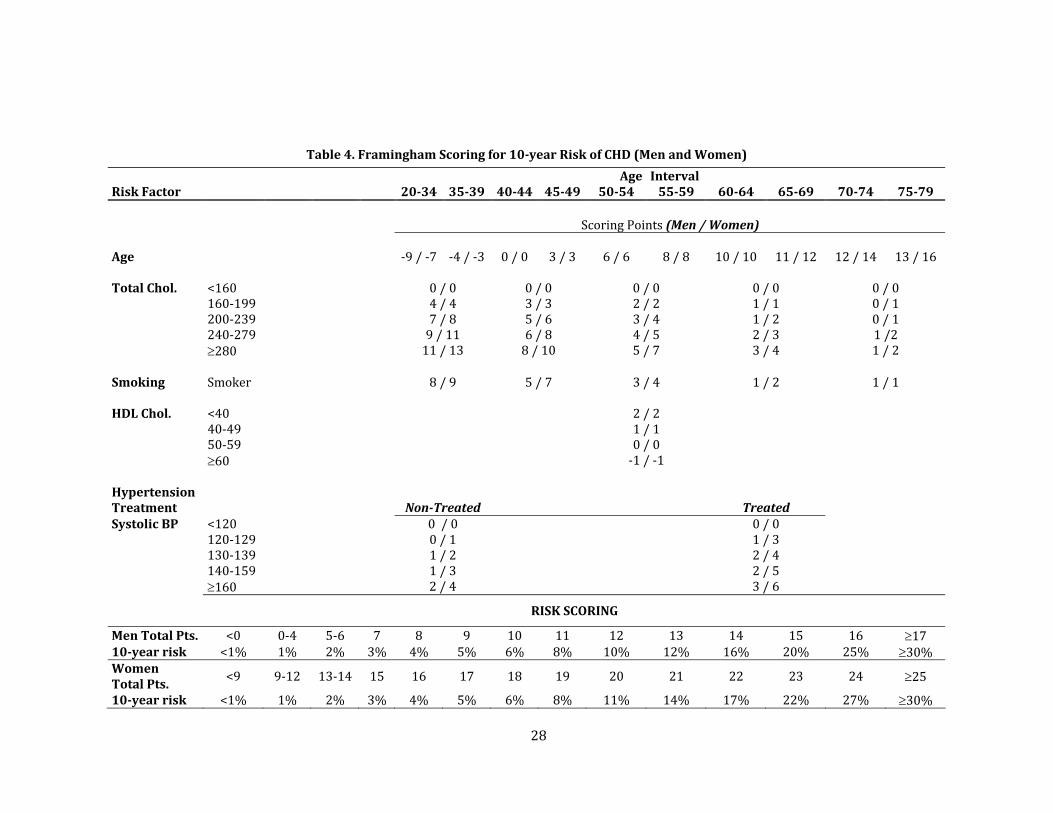
3.2.3 Framingham Risk Score (FRS)

I compute the 10‐year risk of coronary heart disease (CHD) by using the 2001 Framing‐

ham  point  system  guidelines  from  the  National  Cholesterol  Education  Program  (NCEP 

2001). The risk factors included in FRS are age, total cholesterol, HDL cholesterol, systolic 

blood pressure, tobacco smoking, and treatment for hypertension.   Table 4 shows the FRS 

scoring system for men and women.  For example, a 77‐year‐old man who is a smoker, has 

total cholesterol equal  to 170, HDL cholesterol equal  to 30, and non­treated  systolic BP of 

125, will have an FRS score of 16, which translates into a 10‐year risk of CHD equal to 25%.  

Since  this  scoring  system has  only  been  validated  for  individuals  of  age  20‐79,  I  conduct 

these analyses only with NHANES respondents within that age range.  A potential  source of 

confusion in the terminology when using the Framingham scoring system is the fact that the 

algorithm produces a point total which then is mapped into an estimate of 10‐year risk of 

coronary heart disease.  Unless otherwise noted, whenever I allude to the Framingham score 

or Framingham risk score, the reference is to the 10‐year risk of CHD. 

 

28 

Table 4. Framingham Scoring for 10­year Risk of CHD (Men and Women) 

Risk Factor          20­34  35­39  40­44  45­49 Age 

50­54 Interval 55­59  60­64  65­69  70­74  75­79 

                     Scoring Points (Men / Women)                              Age          ‐9 / ‐7 ‐4 / ‐3 0 / 0  3 / 3  6 / 6  8 / 8  10 / 10  11 / 12  12 / 14  13 / 16                    Total Chol.  <160        0 / 0  0 / 0  0 / 0  0 / 0  0 / 0   160‐199        4 / 4  3 / 3  2 / 2  1 / 1  0 / 1   200‐239        7 / 8  5 / 6  3 / 4  1 / 2  0 / 1   240‐279        9 / 11  6 / 8  4 / 5  2 / 3  1 /2   280        11 / 13  8 / 10  5 / 7  3 / 4  1 / 2                    Smoking  Smoker        8 / 9  5 / 7  3 / 4  1 / 2  1 / 1                    HDL Chol.  <40            2 / 2       40‐49            1 / 1       50‐59            0 / 0       60            ‐1 / ‐1                              Hypertension  Treatment  

       Non­Treated          Treated 

   

Systolic BP  <120        0  / 0          0 / 0       120‐129        0 / 1          1 / 3       130‐139        1 / 2          2 / 4       140‐159        1 / 3          2 / 5       160        2 / 4          3 / 6       

RISK SCORING 

Men Total Pts.  <0  0‐4  5‐6  7  8  9  10  11  12  13  14  15  16  17 10­year risk  <1%  1%  2%  3%  4%  5%  6%  8%  10%  12%  16%  20%  25%  30% Women Total Pts. 

<9  9‐12  13‐14 15  16  17  18  19  20  21  22  23  24  25 

10­year risk  <1%  1%  2%  3%  4%  5%  6%  8%  11%  14%  17%  22%  27%  30% 

 

29 

 

3.2.4 Imputation of Income Categories

Most control variables used in this study are missing values for relatively few observa‐

tions and thus the removal of those observations from the sample is not a source of concern 

in terms of potential bias in the results.  One exception is the ratio of family income to pov‐

erty level (PIR), which is missing for 1,827 of the 20,608 observations, almost 9 percent of 

the study sample.   

In  order  to  prevent  the  exclusion  of  so many  observations,  I  use  a  single  imputation 

method (Donders et al. 2006).   The imputation procedure is the following: First, using ob‐

served values, I create six PIR categories (PIR<1.0, 1.0PIR<2.0, 2.0PIR<3.0, 3.0PIR<4.0, 

4.0PIR<5.0, and PIR5.0).    I  then estimate an ordinal  logistic model of the PIR categories 

on a set of socio‐demographic variables (age, gender, ethnicity, education, health insurance, 

employment status, type of work done the longest, and marital status), and for each obser‐

vation in the sample missing a value of PIR I predict the probabilities of it belonging to each 

of the six PIR categories.  Finally, to introduce an element of uncertainty—and thus realism, 

since not all individuals with, for example, a college education are at the top of the income 

scale—I generate a random variable with a uniform distribution between zero and one, and 

impute  the  PIR  category  of  those  observations  missing  PIR  according  to  the  cumulative 

probabilities of belonging in each category and the random number corresponding to that 

observation.8  

                                                             

8 For example, if an observation has probabilities 0.10, 0.20, 0.40, 0.15, 0.10, and 0.05 of belonging in PIR categories 1‐6, respectively, and the random number generated  for  that observation  is 0.6,  the imputed PIR category for that observation will be PIR3, but  if  the random number  is 0.97 then the imputed  category  will  be  PIR6.    Thus,  this  observation  has  a  relatively  large  probability  of  being placed in category PIR3, but this result is not deterministic. 

 

  ‐ 30 ‐ 

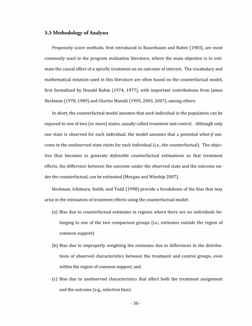
3.3 Methodology of Analyses

Propensity score methods,  first  introduced  in Rosenbaum and Rubin (1983), are most 

commonly used  in  the program evaluation  literature, where  the main objective  is  to  esti‐

mate the causal effect of a specific treatment on an outcome of interest.  The vocabulary and 

mathematical notation used in this literature are often based on the counterfactual model, 

first  formalized by Donald Rubin  (1974,  1977), with  important  contributions  from  James 

Heckman (1978, 1989) and Charles Manski (1995, 2003, 2007), among others. 

In short, the counterfactual model assumes that each individual in the population can be 

exposed to one of two (or more) states, usually called treatment and control.   Although only 

one state  is observed  for each  individual,  the model assumes  that a potential what­if  out‐

come in the unobserved state exists for each individual (i.e., the counterfactual).  The objec‐

tive  thus  becomes  to  generate  defensible  counterfactual  estimations  so  that  treatment 

effects, the difference between the outcome under the observed state and the outcome un‐

der the counterfactual, can be estimated (Morgan and Winship 2007). 

Heckman, Ichimura, Smith, and Todd (1998) provide a breakdown of the bias that may 

arise in the estimation of treatment effects using the counterfactual model:  

(a) Bias due to counterfactual estimates  in regions where there are no  individuals be‐

longing  to one of  the  two  comparison groups  (i.e.,  estimates outside  the  region of 

common support) 

(b) Bias due  to  improperly weighting  the estimates due  to differences  in  the distribu‐

tions  of  observed  characteristics  between  the  treatment  and  control  groups,  even 

within the region of common support, and 

(c) Bias  due  to  unobserved  characteristics  that  affect  both  the  treatment  assignment 

and the outcome (e.g., selection bias). 

 

  ‐ 31 ‐ 

Matching  is  a  commonly  used  approach  that  eliminates  the  first  two  sources  of  bias 

(Blundell, Dearden, and Sianesi 2005).  Its basic idea is to generate a sample of individuals 

in the control state with a distribution of characteristics that closely resembles that of indi‐

viduals in the treatment state.  If the assumption of selection on observables holds,  the third 

source  of  bias  listed  above  is  ignorable  and  the  differences  in  outcomes  between  both 

groups can be attributed to the treatment. 9   

If the set of variables used to do the matching is large, finding exact matches can be dif‐

ficult.  Matching on the propensity score is an alternative to reduce the high dimensionality 

of this problem.  The propensity score is simply the probability that an individual is in the 

treatment group, given the set of observed characteristics that are related to both treatment 

status and outcome; Rosenbaum and Rubin (1983) showed that matching on the propensity 

score  achieves  the  same  results  as  matching  on  the  complete  set  of  observed  variables.  

More recently, methods that use the propensity scores as weights, rather than matching on 

them, have been developed.  In Section 3.3.1, I discuss combining propensity score weight‐

ing and regression, the method I use in this study; a fairly comprehensive review of these 

and other “treatment effects” methodologies can be found in Imbens (2004). 

As I mentioned above, propensity score methods are mostly used in the context of pro‐

gram evaluation, where the counterfactual is clearly defined—that is, some individuals re‐

ceive  the  treatment  but  might  not  have  received  it,  just  as  those  who  did  not  get  the 

treatment could have received it; thus, in most propensity score applications, individuals in 

the treatment group could have been in the control group and vice versa.  However, Frölich 

                                                             

9  The  selection  on  observables  condition,  often  also  called unconfoundedness,  requires  that,  condi‐tionally  on  the  observed  variables,  the  distribution  of  the  counterfactual  outcome  in  the  treated group is the same as the observed distribution of the outcome in the control group.   This condition implies  that unobserved variables  that  affect  the outcome  should not  also affect  treatment  assign‐ment. 

 

  ‐ 32 ‐ 

(2007) shows that propensity score methods can be used outside the sphere of treatment 

evaluation because the consistency of these methods does not depend on the concept of the 

counterfactual.  Frölich, for example, uses propensity score matching to analyze the gender 

wage gap  in  the United Kingdom, where  the  treatment group are women, and  the control 

group are men. 

Although propensity score methods are often used as an alternative to regression analy‐

sis,  both  methods  depend  on  the  principle  of  unconfoundedness  (i.e.,  ignorability  of  the 

third source of bias described above).  There are, however, two key differences.  First, pro‐

pensity  score  methods  can  be  nonparametric  or  semiparametric,  depending  on  how  the 

propensity  score  is  estimated,  while  linear  regression makes  the  assumption  that  condi‐

tioning on a linear combination of the covariates is enough to eliminate selection bias; if the 

covariate distributions are  similar  enough between both groups,  the  linearity  assumption 

may  not  be  important,  but  if  the  distributions  differ  substantially,  parameter  estimations 

may  be  based mostly  on  extrapolations,  with  the  potential  for  substantial  bias.    Second,  

propensity  score methods allow  for a  straightforward  identification of  the  region of  com‐

mon  support,  highlighting  the  importance  of  removing  individuals  from  the  control  (or 

treatment)  group who  do  not  have  similar  counterparts  in  the  other  group;  this  issue  is 

usually  ignored  in  studies  that  use  regression methods,  letting  the  linear  functional  form 

produce estimates outside the region of common support (Caliendo 2006).    If overlap is a 

problem, however, neither regression methods nor propensity score models are appropri‐

ate, but common regression diagnostics do not focus on assessing this situation. 

Nevertheless, it is important to note that if the assumptions of regression methods are 

met—particularly,  if  the  specification  of  the  functional  form  is  correct  and  the  region  of 

common support covers the entire range of the data—the use of propensity score methods 

will  not  provide  any  benefits  over  regression  in  terms  of  unbiased  estimation  of  the  pa‐

 

  ‐ 33 ‐ 

rameters.  Still, under uncertainty, using propensity score methods has distinct advantages 

due to the key differences described in the previous paragraph (Rubin 1997; Harding 2003).   

3.3.1 Doubly-Robust Estimator: Propensity Score-Weighted Regression

Although  both  regression  and  propensity  score  methods  are  used  for  the  same  pur‐

pose—to  reduce  estimation  bias  related  to  differences  in  observed  covariates—there  are 

potential advantages to combining them (Rubin and Thomas 2000; Ho et al. 2007).   James 

Robins refers to the combination of propensity score and regression methods as a “doubly 

robust” estimator in the sense that, as long as the parametric model for either the propen‐

sity  score or  the outcome regression  is  correctly  specified,  the  resulting estimator will be 

consistent.    Thus,  combining propensity  score weighting with  regression provides  the  re‐

searcher with  “two  chances”  to  get nearly  correct  inference  about  a  causal  effect  (Robins 

and Rotnitzky 2001; Bang and Robins 2005). 

The approach I use in this study roughly mirrors that of Hirano and Imbens (2001), who 

propose  an  estimator  that  combines  propensity  score  (PS) weighting with  regression  ad‐

justment.  Specifically, I first estimate the propensity score model using a logistic regression 

of the form:10    

 

expPr 1 .

1 expi i

zM Z z

z

  (3) 

                                                             

10 In practice, the choice of a logistic or probit model is not critical, since both models produce similar results (Caliendo and Kopeinig 2008).  However, since I use bootstrapping techniques to estimate the standard  errors  of  the  estimators  (more details  below  in  this  section),  I  choose  the  logistic model because its computation is slightly faster. 

 

  ‐ 34 ‐ 

In this equation,  iM is an indicator equal to one when the individual is of Mexican eth‐

nicity and zero otherwise;11  iZ is a vector of covariates that vary across Mexicans and non‐

Mexicans; and  is a vector of regression coefficients.   Once this regression is estimated, I 

compute a propensity score,  ˆ ,ip z for every observation in the sample by predicting each 

individual’s likelihood of being Mexican given her observed covariate values.  To guarantee 

that estimates are computed  in  the region of common support,  I drop observations  in  the 

Mexican sample with higher propensity scores than the maximum propensity score value in 

the comparison sample and, similarly,  I drop observations  in  the comparison sample with 

propensity score values below the minimum propensity score in the Mexican sample. 

After computing the propensity scores and limiting the sample to the region of common 

support, I estimate the average difference in allostatic load and Framingham risk scores be‐

tween Mexicans and  the comparison groups using  two different methods:   First,  I use  the 

traditional  semiparametric approach—where  the propensity  scores are estimated using a 

parametric model, but no specific  functional  form is assumed for the allostatic  load differ‐

ences between groups—by taking a simple difference  in means between both groups, but 

weighting each observation with the following weights: 

 

ˆ, 1 ,

ˆ1i

i i i ii

p zw m w v m m

p z

  (4) 

where iv are  the  NHANES  sampling  weights,  and  im and  ˆ ip z are  defined  the  same  as 

above.  Thus, the PS weights are equal to one (multiplied by the sampling weights) for Mexi‐

                                                             

11  My analyses involve four different comparisons: (a) Whites with all Mexicans, (b) Whites with US‐born Mexicans, (c) Whites with Mexican immigrants, and (d) US‐born Mexicans with Mexican immi‐grants; thus,  iM is defined accordingly to the relevant comparison, with Mexican immigrants being the treatment group in the last of the four comparisons. 

 

  ‐ 35 ‐ 

cans and  ˆ ˆ1i ip z p z  for the individuals in the comparison group.  The semiparamet‐

ric estimator of allostatic load differences between groups is then equal to: 

  11,

1 1

ˆct

t c

nnj ji i ji

a s n n

i ji j

w ALw AL

w w

  (5) 

Similarly, the semiparametric estimator of Framingham risk score (FRS) differences be‐

tween groups is:12  

  11,

1 1

ˆct

t c

nnj ji i ji

f s n n

i ji j

w FRSw FRS

w w

  (6) 

Second, I compute the doubly‐robust estimator of differences between ethnic groups by 

estimating least squares regressions with the form: 

  0 , 1 2 1ˆi a p i i i i iAL M X M X X   (7) 

where  iAL is the allostatic load score of individual i;  ,ˆa p is the doubly‐robust parametric 

estimator of the difference in allostatic load between Mexicans and Whites (or the relevant 

comparison  group);  iX is  a  vector  of  socioeconomic  and  demographic  covariates;  and 

1X is the average of  X for the relevant treatment group (i.e., all Mexicans, US‐born Mexi‐

cans, or Mexican immigrants).  The same PS weights in equation (4) are used to weigh the 

observations in these regressions. 

I should observe that I do not produce a doubly‐robust estimator for the FRS measure 

because the Framingham 10‐year risk of CVD is top‐coded at 30%—that is, for individuals 

                                                             

12 As  explained  in  section 3.2.3,  the outcome variable  in  these  analyses  is  the 10‐year  risk of CHD computed using the scoring system in Table 4.  For simplicity, I refer to this risk as the Framingham risk score (FRS). 

 

  ‐ 36 ‐ 

with 10‐year risk of CHD above 30% I do not have an exact risk estimate, I only know that it 

is at least 30%.  A common method to conduct analyses when the outcome measure is top‐

coded  (i.e.,  right‐censored)  is  the  Tobit  regression model  (Tobin  1958;  Schnedler  2005).  

Indeed, I could substitute this method for the ordinary least squares model in order to com‐

pute  the  doubly‐robust  estimator.    However,  Tobit models  require  stronger  assumptions 

than ordinary least squares and are particularly vulnerable to biases in the presence of het‐

eroskedasticity (Johnston and DiNardo 1997).  In order to avoid these problems, I limit the 

analyses using the Framingham score to the semiparametric estimator in equation (6).   

The specification  in equations (4) – (7) produces an estimation of  the treatment effect 

for the treated (ATT); that is, the estimators  , ,ˆ ˆ, ,a s f s  and  ,ˆa p represent the average differ‐

ence  in  allostatic  load—or  Framingham  risk  scores—between Mexicans  and  a  sample  of 

Whites with a covariate distribution similar to the Mexican sample.  I consider this estima‐

tor to be more appropriate for this study than the more commonly used average treatment 

effect (ATE), which estimates the average difference between Mexicans and a sample with a 

covariate distribution similar to that of the entire sample. 

A final important issue when propensity score methods are used is that the standard er‐

rors estimated by statistical software in the final step—equations (6) and (7)—are incorrect 

because  the propensity score estimation  in  the  first step and  the use of PS weights  in  the 

second step  introduce additional  sources of variability  that are not  taken  into account by 

the software that estimates either the differences in means or the WLS equation.  Correctly 

estimating the standard errors is important in order to test the significance of the parame‐

ter  estimates.    Following  a  common  approach  in  the  literature  (Caliendo  and  Kopeinig 

2008), I use bootstrapping to estimate the standard errors of the main parameter estimates.  

For each of the four comparisons, 250 bootstrap draws are conducted, each of them repro‐

ducing the entire procedure described in this section; that is,  in each repetition: (1) a new 

 

  ‐ 37 ‐ 

sample with  replacement  is  drawn,  (2)  the propensity  scores  are  computed,  (3)  observa‐

tions outside the region of common support are dropped, (4) propensity score weights are 

generated, (5) the average difference between Mexicans and the comparison group is esti‐

mated  using  a  PS‐weighted  difference  in means,  and  (6)  the  adjusted  difference  between 

Mexicans and the comparison group is estimated using a PS‐weighted least squares regres‐

sion. 

3.3.2 Model Building

Choosing  the  sets  of  covariates  to  be  included  in  the  propensity  score  and  outcome 

models (equations (3) and (7)) is not a straightforward decision.  Some authors suggest in‐

cluding  a  comprehensive  set  of  covariates  and  advise  against  removing  variables  when 

doubt exists about whether they should be included or not (e.g., Rubin and Thomas 1996).  

Conversely, others argue that the choice of variables must be made carefully and taking into 

account theory, previous research, and any additional knowledge relevant to the particular 

model being estimated (Caliendo and Kopeinig 2008).   

Regardless of the approach used to build the models, since the main objective of using a 

propensity  score method  is  to balance  the distribution of  characteristics  in  the  treatment 

and  control  groups,  one  should  always  assess  the  quality  of  the  matching  method  used.   

There are several alternatives to do this, but I choose the simplest one, which is to conduct 

two‐sample t‐tests to check  if  there are any significant differences  in the means of  the co‐

variates in the treatment and control groups.  If the t‐test shows significant differences, then 

the propensity score model is misspecified and higher‐order terms and interactions of the 

original covariates must be added to the model until the differences in covariate means are 

no longer significant. 

 

  ‐ 38 ‐ 

The  strategy  I  choose  to build  the propensity  score and outcome models  is  similar  to 

that  described  in  Hirano  and  Imbens  (2001),  who  estimate  k  logistic  regressions  of  the 

treatment dummy on each individual covariate (where k is the number of covariates avail‐

able  in  their data)  and similarly estimate k  ordinary  least  squares  regressions of  the out‐

come  variable  on  the  treatment  dummy  and  each  covariate.    They  then  include  in  the 

propensity score model all covariates with a t‐statistic above a threshold value  pt , and they 

include in the outcome model all covariates with a t‐statistic above a threshold value  .regt   

Although this method is easy to implement, it ignores issues such as the inclusion of poten‐

tially  endogenous  covariates  in one of  the models,  or  correlation between  covariates  that 

may  lead  to multicollinearity.    I  thus  estimate k  logistic  and OLS  regressions,  but use  the 

results only as guides to identify covariates that are clearly not significant in either the pro‐

pensity  score or outcome models  and  to make decisions  regarding  the  collapsing of  cate‐

gorical variables  into  fewer groups.   Following the suggestions of other authors (Caliendo 

and Kopeinig 2008),  I  include  in  the outcome model variables  that previous  research has 

shown to be significantly associated with health outcomes.   

An additional complication I face is the fact that in this study I estimate a large number 

of outcome models: since I have four sets of comparisons (see footnote 11) and five sets of 

outcomes  (allostatic  load,  inflammatory,  metabolic,  cardiovascular,  and  Framingham  risk 

scores), my main analyses require the estimation of 20 models;  in addition, my sensitivity 

analyses  (see  Section  3.3.3)  involve  similar  estimations  using  a  different  definition  of  al‐

lostatic  load,  previously  used  by  other  authors;  finally,  I  conduct  additional  estimations 

where  I  remove  from  the models variables  that  are potentially endogenous.    In all,  I  esti‐

mate a total of 100 models.  In order to simplify model selection, I include in each model all 

covariates with  significant  t‐tests  in  any  of  the  five  outcomes,  regardless  of  whether  the 

 

  ‐ 39 ‐ 

covariate is significant in each particular model or not.   Finally, I include in the propensity 

score models all covariates present in the outcome models to guarantee that their distribu‐

tions are balanced across the treatment and control groups. 

3.3.3 Sensitivity Analyses

3.3.3.1 Traditional Definition of Allostatic Load

Many  recent  studies  have  defined  the  AL  measure  as  a  count  of  the  number  of  bio‐

markers with values beyond a certain threshold of high risk (see Section 3.1.1 above).  As I 

also commented earlier, these measures implicitly assign each biomarker the same impor‐

tance and do not account for potential non‐linearities in the relationship between the bio‐

markers and, say, mortality.  Nevertheless, in order to assess the sensitivity of my results to 

the definition of allostatic load (and its three subcomponents) used in this study, I estimate 

weighted‐least squares models—with the propensity score weights—in which the allostatic 

load variables are defined as in these studies.   

In this definition, subjects are classified for each biomarker into quartiles based on the 

distribution of scores in the sample.  The traditional allostatic load score is created by sum‐

ming  the number  of  biomarkers  in  the highest  risk quartile, which  is  the  top quartile  for 

most of the eight biomarkers, except for HDL cholesterol and albumin, for which the bottom 

quartile is the highest risk group.  A similar procedure is used to create summary scores for 

the inflammatory, metabolic, and cardiovascular systems.  

 

  ‐ 40 ‐ 

3.3.3.2 Potential Endogeneity of Covariates

Although  the main variable of  interest—Mexican ethnicity—is  clearly not endogenous 

in the allostatic load models because health status does not determine whether a person is 

Mexican or not,13  some of  the  control  variables used  in both  the propensity  score and al‐

lostatic load models (e.g., income, education) are likely to be endogenous either in the pro‐

pensity  score or  in  the outcome models.    For  example, Mexicans  are more  likely  to  come 

from families with low income and are less likely to have health insurance.   Since both in‐

come and insurance status are used in the allostatic  load models as control variables,  it  is 

possible that the coefficient estimates of the main variable of interest are biased.  In order to 

assess the importance of this problem, I estimate the models in Section 3.3.1 with and with‐

out the income and insurance variables. 

3.4 Results

3.4.1 Construction of Allostatic Load Measure

The results of the survival and logistic regressions are shown in Table 5.  Only the fourth 

and  fifth quintiles are used  for C‐reactive protein because 60 percent of  the observations 

had  the  same value due  to  the  lowest possible measurement  in NHANES‐III,  and  thus  the 

first three quintiles are the reference group in that case.14  The association of the eight bio‐

markers with mortality varies significantly  in  terms of strength and direction.   The coeffi‐

                                                             

13 Endogeneity would be a concern if certain individuals were less likely to report being of Mexican ethnicity and their health status were different from those who do report being Mexican.  Although a similar problem has been mentioned in studies that use death records to explore the Hispanic Para‐dox, I am not aware of any study that has found that ethnicity self‐reporting varies across individuals of different health statuses. 

14  The  lowest  measured  CRP  value  in  the  1999‐2004  NHANES  was  significantly  lower  than  in NHANES‐III.    To  avoid  spurious  results  that  lower  CRP  values  in  the  latter  NHANES  imply  better health than in NHANES‐III, I set the minimum CRP value in 1999‐2004 equal to that of NHANES‐III, which resulted in 60% of the observations having this value. 

 

  ‐ 41 ‐ 

cients  in  Table  5  show mostly  the  expected  results:  allostatic  load  increases with  higher 

values of C‐reactive protein, glycosylated hemoglobin,  total cholesterol, pulse, and systolic 

blood pressure; allostatic load decreases with higher values of serum albumin; and, finally, 

the  association  of  allostatic  load with  diastolic  blood  pressure  and HDL  cholesterol  is  U‐

shaped,  with  low  (high)  values  of  diastolic  BP  (HDL  cholesterol)  being  associated  with 

higher AL than values in the middle.   Despite the U‐shaped relationship, HDL values in the 

fifth quintile are still better than HDL values in the first quintile, as would be expected. The 

relative magnitudes of  the coefficients are similar  in both the survival and  logistic regres‐

sions and most signs are identical (the only one that is different, fourth quintile of HDL cho‐

lesterol, is not significant in either regression.  Given the overall consistency of the results, I 

conclude the coefficients are robust and I use those estimated in the survival regression as 

weights  in  the  allostatic  load  score,  since  the  survival  models  use  the  most  information 

available from the data.  

Allostatic  load is thus defined as a  linear combination of the quintiles of the eight bio‐

markers, where the linear combination’s weights are the coefficients estimated in the sur‐

vival regressions.  Using equation (2), an individual’s allostatic load score is: 

 

 

4 5 1 2 4 5

1 2 4 5 1 2 4 5

1 2 4 5 1 2 4

0.35 0.92 0.93 0.32 0.22 0.81

0.58 0.29 0.59 1.40 0.47 0.14 0.23 0.64

0.40 0.12 0.09 0.26 0.18 0.23 0.13 0.45

iAL crp crp alb alb alb alb

gly gly gly gly tch tch tch tch

hdl hdl hdl hdl pul pul pul pul

5

1 2 4 5 1 2 4 50.68 0.40 0.54 1.58 0.24 0.01 0.03 0.25sys sys sys sys dia dia dia dia

   (8) 

 

Recall that, for example,  4crp is a dummy variable equal to one if the respondent is in 

CRP’s fourth quintile and zero otherwise, so that only one coefficient from each biomarker’s 

set of dummy variables will be used in the AL score.  Thus, an individual with values of all 

 

  ‐ 42 ‐ 

eight biomarkers in the middle quintile would have an allostatic load score of zero.  Higher 

allostatic  load  scores  represent worse  health.    For  ease  of  interpretation  of  the  results,  I 

transform the AL, inflammatory, metabolic, and cardiovascular scores so that each of them 

has a mean of zero and standard deviation equal to one.  I use these standardized variables 

in all remaining analyses. 

3.4.2 Descriptive Statistics

The descriptive statistics of the original sample of NHANES participants, weighted using 

the original NHANES sampling weights, are shown in Table 6.  Clearly, there are significant 

differences in the distributions of covariates between Whites and Mexicans.  The latter are, 

on average, almost ten years younger, have lower income, are less educated, and are more 

likely to have had blue collar jobs.  Moreover, there are also significant differences between 

US‐born Mexicans  and Mexican  immigrants.    The  characteristics  of US‐born Mexicans  are 

generally at  a midpoint between  those of Whites and Mexican  immigrants.   An  important 

characteristic of Mexican immigrants is that only 42 percent of them are female, compared 

to  51  percent  for  both Whites  and  US‐born Mexicans.    Differences  in  education  are  also 

striking: over 70 percent of Mexican  immigrants do not have a high school diploma, com‐

pared to 17 percent of Whites and 33 percent of US‐born Mexicans. 

 

 

 

  ‐ 43 ‐ 

Table 5. Estimated Coefficients from Survival Models for Allostatic Load Weights 

Biomarker  Quintile  Survival Models  Logistic Models  Shape 1st  See note  See note 2nd  See note  See note 3rd  Reference  Reference 4th  0.350  (0.107)  0.209 (0.119) 

CRP 

5th  0.920  (0.068)  0.904  (0.705) 

Increasing 

             

1st  0.933  (0.098)  0.844  (0.107) 2nd  0.321  (0.099)  0.315  (0.100) 3rd  Reference  Reference 4th  ‐0.221 (0.133)  ‐0.174 (0.133) 

Albumin 

5th  ­0.811  (0.160)  ­0.709  (0.168) 

Decreasing 

             

1st  ­0.579  (0.150)  ­0.552  (0.142) 2nd  ­0.289  (0.127)  ‐0.253 (0.133) 3rd  Reference  Reference 4th  0.589  (0.115)  0.609  (0.121) 

Glycosylated Hemoglobin 

5th  1.398  (0.097)  1.451  (0.103) 

Increasing 

             

1st  ­0.469  (0.107)  ­0.485  (0.106) 2nd  ‐0.140 (0.101)  ‐0.161 (0.109) 3rd  Reference  Reference 4th  0.225  (0.103)  0.229  (0.111) 

Total  Cholesterol 

5th  0.643  (0.093)  0.679  (0.093) 

Increasing 

             

1st  0.398  (0.115)  0.414  (0.116) 2nd  0.119 (0.105)  0.137 (0.107) 3rd  Reference  Reference 4th  ‐0.090 (0.114)  0.088 (0.117) 

HDL Cholesterol 

5th  0.258  (0.105)  0.264  (0.114) 

U­Shaped 

             

1st  ‐0.182 (0.111)  ‐0.140 (0.118) 2nd  ‐0.232 (0.125)  ‐0.216 (0.134) 3rd  Reference  Reference 4th  ‐0.132 (0.144)  ‐0.153 (0.149) 

Pulse 

5th  0.448  (0.119)  0.421  (0.130) 

Flat, then  Increasing 

             

1st  ­0.683  (0.137)  ­0.710  (0.139) 2nd  ­0.404  (0.135)  ­0.438  (0.142) 3rd  Reference  Reference 4th  0.536  (0.101)  0.567  (0.105) 

Systolic Blood  Pressure 

5th  1.577  (0.103)  1.694  (0.109) 

Increasing 

         

1st  0.238  (0.102)  0.195 (0.103) 2nd  0.007 (0.112)  0.018 (0.119) 3rd  Reference  Reference 4th  ‐0.030 (0.104)  ‐0.024 (0.109) 

Diastolic Blood  

Pressure 5th  0.250  (0.086)  0.276  (0.086) 

U­Shaped 

NOTES:  Standard errors are  in parentheses.    Coefficients  in bold  typeface  are  significant  at  the 5 percent  confidence  level.    The  survival  regressions  are  semi‐parametric  Cox  proportional  hazards models. Due to the minimum level measured in NHANES‐III, about 60% of the observations have the same C‐reactive protein (CRP) value; thus, the first three quintiles are used as reference. 

 

 

  ‐ 44 ‐ 

Table 6. Descriptive Statistics of Original Sample (Averages/Proportions) 

Variable  Whites  All Mexicans US­born  Mexicans 

Mexican  Immigrants 

N (unweighted)  12,778 6,583 3,095  3,488   Age      47 38 40  37Female  51% 46% 51%  42%Income/Pov. Ratio       PIR < 1.0  9% 29% 21%  36%    1.0  PIR < 2.0  18% 34% 26%  39%    2.0  PIR < 3.0  19% 16% 18%  15%    3.0  PIR < 4.0  17% 9% 14%  6%    4.0  PIR < 5.0  13% 5% 8%  2%    PIR > 5.0  24% 7% 13%  2%Education       Less than HS  17% 55% 33%  71%    HS degree  35% 24% 34%  17%    College +  48% 21% 33%  12%Insurance       Private  78% 45% 61%  33%    Public  11% 12% 15%  10%    Uninsured  11% 43% 24%  57%Type of work done the longest 

 

    Never worked  2% 5% 3%  7%    White collar   26% 8% 13%  5%    Service   42% 36% 47%  28%    Blue collar   29% 50% 35%  60%    Military  1% 1% 2%  0%Marital Status       Single  14% 19% 20%  19%    Widowed/Divorced  18% 12% 16%  9%    Married  68% 69% 64%  72%

NOTES: All observations are weighted using the original NHANES sampling weights for the sample that received medical examinations.  The sample size of US‐born Mexicans and Mexican immigrants does not add up to the total of all Mexicans in the sample because a few respondents reported Mexi‐can ethnicity but not their country of birth. 

 

Average values of  the biomarkers  included  in  the allostatic  load  index  for each ethnic 

group are shown in Table 7.  Mexican immigrants have the ‘best’ average values in six of the 

biomarkers used in this study—C‐reactive protein, serum albumin, total cholesterol, pulse, 

systolic blood pressure, and diastolic blood pressure—, while Whites had the best average 

values of serum albumin and HDL cholesterol.  Table 7 also shows the average values of the 

 

  ‐ 45 ‐ 

summary  indices  of  health  status.    Mexican  immigrants  have  the  lowest  allostatic  load 

scores, while US‐born Mexicans and Whites have  the highest  (recall  that  lower AL values 

are better, and the scores are centered around the mean, such that the average  in the  full 

sample equals zero).  Not only do immigrants have the lowest overall allostatic load score, 

their inflammatory and cardiovascular scores are also the lowest among the three groups, 

although their metabolic score is slightly higher  (but not statistically significant) than that 

of Whites.  As for the Framingham risk score, Whites have the highest 10‐year risk of coro‐

nary heart disease, (5.1 percent), followed by US‐born Mexicans (3.6 percent), and Mexican 

immigrants (2.7 percent). 

Table 7.  Average Values of Eight Biomarkers, The Allostatic Load Index and its Subcompo­nents, and Framingham Risk Score; by Ethnic Group 

 Non­Hispanic  

Whites US­Born  Mexicans 

Mexican  Immigrants 

C­reactive  Protein 

0.419  (0.007) 0.516 (0.027)  0.414  (0.014)

Serum Albumin*  4.285 (0.013) 4.308 (0.023)  4.351  (0.013)Glycosylated  Hemoglobin 

5.338  (0.016) 5.464 (0.024)  5.469  (0.024)

Total Cholesterol  203.1 (0.599) 196.3  (1.153)  194.8  (1.062)HDL Cholesterol*  51.30  (0.272) 50.56 (0.302)  48.15  (0.279)Pulse  73.34 (0.249) 73.86 (0.392)  71.09  (0.278)Systolic Blood  Pressure 

121.6 (0.302) 119.9 (0.573)  117.2  (0.484)

Diastolic Blood  Pressure 

72.32 (0.196) 71.93 (0.312)  69.57  (0.354)

     Allostatic Load  0.065 (0.045) 0.065 (0.028)  ­0.137  (0.030)    Inflammatory Score  0.049 (0.031) 0.109 (0.055)  ­0.147  (0.031)    Metabolic Score  0.055 (0.025) 0.078 (0.035)  0.061  (0.030)    Cardiovascular Score  0.040 (0.018) ‐0.016 (0.035)  ­0.226  (0.030)Framingham Risk Score  5.08% (0.108) 3.59% (0.138)  2.72%  (0.148)NOTES: Standard errors are in parentheses.  * Indicates biomarkers for which higher values rep‐resent better health status.   Bold  typeface indicates the group with the  ‘best’ average value for each biomarker.    If  the differences between any group and the  ‘best’ group are not statistically significant, both are in bold typeface. 

 

  ‐ 46 ‐ 

3.4.3 Common Support

A first assessment of the region of common support can be made visually, by inspecting 

the distribution of propensity scores  in the treatment and control groups (Lechner 2000).  

The main goal of this initial assessment is to spot any potential support problems, and then 

one can proceed to do a more precise assessment of the common support region and elimi‐

nate observations outside of it.   

The distributions of the propensity scores in each of the four comparisons are shown in 

Figure  2.15      Although  the  propensity  score  distributions  of  the White  sample  in  the  first 

three graphs have “thin” right tails, there is sufficient overlap between treatment and con­

trol groups in all four comparisons—the last graph is for the comparison of US‐born Mexi‐

cans and Mexican  immigrants.    In order  to guarantee  that  the common support  condition 

holds,  I  apply  the  method  of  comparing  minimum  and  maximum  values  (Caliendo  and 

Kopeinig  2008).    That  is,  I  delete  all  observations with  lower  propensity  scores  than  the 

minimum—and higher propensity scores than the maximum—in the opposite group.    

The minima and maxima of the propensity scores, as well as the number of observations 

dropped due to being outside the common support region, are reported in Table 8.  Not sur‐

prisingly, the comparison with the most dropped observations was that for Mexican immi‐

grants and Whites, and even in that comparison less than 3 percent of the sample had to be 

dropped.  Despite the considerable differences in the distribution of covariates reported in 

Table  6,  the  number  of  observations  outside  the  region  of  common  support  is  relatively 

small.  Thus, common support does not appear to be a problem and valid estimates of health 

differences between the treatment and control groups can be estimated in the common sup­

port region.  

                                                             

15 Non‐parametric kernel methods were used to plot the propensity score distributions. 

 

  ‐ 47 ‐ 

Table 8. Propensity Score Minima/Maxima and Observations Removed from Sample  

Comparison Min/Max Control 

Min/Max Treatment 

Deleted Observations Control/Treatment 

Total Obs.  Remaining 

All Mexicans vs. Whites  0.001/0.76 0.002/0.82  83  27  19,253US­born Mexicans vs. Whites  0.001/0.27 0.002/0.30  37  2  15,834Mexican immigrants vs. Whites  0.000/0.81 0.003/0.88  343  31  15,892US­born Mex. vs. Immigrants  0.001/0.96 0.024/0.97  37  17  6,529

 

3.4.4 Matching Quality

Table 9 reports the characteristics of the four groups after being balanced with the pro‐

pensity score weights  in equation  (4).   Clearly, weighting with  the propensity scores pro‐

duced  samples  with  similar  average  values  in  all  the  variables  for  the  treatment  and 

comparison groups.  Statistical tests found no significant differences in means between the 

treatment and control groups in any of the four comparisons. 

A clearer representation of the balancing of the samples achieved by using the propen‐

sity  score weights  is  depicted  in  Figure  3, which  shows  the  t‐statistics  of  the  differences 

between the comparison groups in all covariates, both before and after weighting the sam‐

ples with the propensity scores.   The Xs represent t‐statistic values of the mean difference 

between the comparison and treatment groups before PS‐weighting, while black dots show 

the  t‐statistic  values  after  PS‐weighting.    None  of  the  t‐statistic  values  after  weighting  is 

greater than 1.5,  less than 3% are greater than 1.0, and 84% are lower than 0.5.   Figure 4 

provides yet another visualization of overall covariate balance.  It shows the distribution of 

the  propensity  scores  before  and  after  weighting  (the  off‐support  observations  are  still 

shown in the left‐hand side graphs, but omitted from those in the right‐hand side).  Overall, 

both figures show that the propensity score weights succeeded in balancing the samples of 

the  comparison  and  treatment  groups  such  that  all  covariates  have  similar  distributions, 

except for the outcome variables (allostatic load and Framingham risk). 

 

  ‐ 48 ‐ 

Figure 2. Common Support Assessment: Distributions of Propensity Scores Before Adjustments 0

12

34

kde

nsity

psp

_me

xam

0 .2 .4 .6 .8x

NHWhite MexAm

Distrib of Prob(MexAm=1) - Before PS-Weighting

 

05

1015

kde

nsity

psp

_me

xus

0 .1 .2 .3 .4x

NHWhite MexUS

Distrib of Prob(MexUS=1) - Before PS-Weighting

 

01

23

45

kde

nsity

psp

_me

xbo

rn

0 .2 .4 .6 .8x

NHWhite MexBorn

Distrib of Prob(MexBorn=1) - Before PS-Weighting

 

0.5

11.

52

kde

nsity

psp

_me

xbo

rn2

0 .2 .4 .6 .8 1x

mexus MexBorn

Distrib of Prob(MexBorn=1) - Before PS-Weighting

 

 

  ‐ 49 ‐ 

Table 9. Descriptive Statistics of Propensity Score­Weighted Samples—Estimated in the Common Support 

 First Weighted 

Sample Second Weighted  

Sample Third Weighted  

Sample Fourth Weighted  

Sample   Whites  Mexicans  Whites  US Mexicans  Whites  Immigrants  US Mexicans  Immigrants 

N (unweighted)  12,695  6,558 12,741 3,093 12,435  3,457 3,058 3,471Age  38  38 40 40 37  37 37 37Female  46%  46% 50% 50% 43%  42% 43% 42%Income/Pov. Ratio         PIR < 1.0  30%  29% 20% 20% 37%  36% 38% 36%    1.0  PIR < 2.0  33%  34% 26% 26% 39%  40% 39% 39%    2.0  PIR < 3.0  16%  16% 18% 18% 15%  15% 13% 15%    3.0  PIR < 4.0  10%  10% 15% 15% 6%  6% 6% 6%    4.0  PIR < 5.0  5%  5% 8% 8% 2%  2% 2% 2%    PIR > 5.0  7%  7% 13% 13% 2%  2% 2% 2%Education         Less than HS  55%  55% 33% 33% 72%  71% 70% 71%    HS degree  24%  24% 34% 34% 16%  17% 17% 17%    College +  21%  21% 33% 33% 12%  12% 13% 12%Insurance         Private  44%  45% 60% 61% 32%  34% 33% 34%    Public  12%  12% 14% 15% 10%  10% 10% 10%    Uninsured  43%  43% 25% 24% 57%  56% 56% 56%Type of work done the longest 

   

    Never worked  6%  5% 3% 3% 9%  7% 7% 7%    White collar   8%  8% 13% 13% 5%  5% 5% 5%    Service   37%  36% 47% 47% 28%  28% 29% 28%    Blue collar   48%  50% 35% 35% 58%  60% 59% 60%Marital Status         Single  19%  19% 20% 20% 18%  19% 20% 19%    Widow/Divorced  12%  12% 15% 15% 9%  9% 11% 9%    Married  69%  69% 65% 65% 72%  72% 69% 72%

 

  ‐ 50 ‐ 

Figure 3. Covariate Balance Before and After Weighting with Propensity Scores 

-20 -10 -2 0 2 10 20t-statistic

Rooms in homeMarried

Widow/Divor.Single

Work: Blue C.Work: ServicesWork: White C.

Work: MilitaryWork: Never

UninsuredIns. Public

Ins. PrivateEdu Coll+

Edu HSEdu LT HS

PIR 5+PIR 4-5PIR 3-4PIR 2-3PIR 1-2PIR < 1Female

AgeMexicans (All) vs. NH White

Original PS-Weighted

 

-10 -5 -2 0 2 5 10t-statistic

Rooms in homeMarried

Widow/Divor.Single

Work: Blue C.Work: ServicesWork: White C.

Work: MilitaryWork: Never

UninsuredIns. Public

Ins. PrivateEdu Coll+

Edu HSEdu LT HS

PIR 5+PIR 4-5PIR 3-4PIR 2-3PIR 1-2PIR < 1Female

AgeUS-born Mexicans vs. NH Whites

Original PS-Weighted

 

-40 -20 -2 0 2 20 40t-statistic

Rooms in homeMarried

Widow/Divor.Single

Work: Blue C.Work: ServicesWork: White C.

Work: MilitaryWork: Never

UninsuredIns. Public

Ins. PrivateEdu Coll+

Edu HSEdu LT HS

PIR 5+PIR 4-5PIR 3-4PIR 2-3PIR 1-2PIR < 1Female

Age

Mexican Immigrants vs. NH Whites

Original PS-Weighted

 

-20 -10 -2 0 2 10 20t-statistic

Rooms in homeMarried

Widow/Divor.Single

Work: Blue C.Work: ServicesWork: White C.

Work: MilitaryWork: Never

UninsuredIns. Public

Ins. PrivateEdu Coll+

Edu HSEdu LT HS

PIR 5+PIR 4-5PIR 3-4PIR 2-3PIR 1-2PIR < 1Female

Age

Mexican Immigrants vs. US-born Mexicans

Original PS-Weighted

 

 

  ‐ 51 ‐ 

Figure 4. Boxplots of the Propensity Scores – Before and After PS­Weighting  

0 .2 .4 .6 .8Pr(mexam)

MexAm

NHWhite

Distrib of Prob(MexAm=1) - Before PS-Weighting

 

0 .2 .4 .6 .8Pr(mexam)

MexAm

NHWhite

Distrib of Prob(MexAm=1) - PS-Weighted

 

0 .1 .2 .3Pr(mexus)

MexUS

NHWhite

Distrib of Prob(MexUS=1) - Before PS-Weighting

0 .05 .1 .15 .2 .25Pr(mexus)

MexUS

NHWhite

Distrib of Prob(MexUS=1) - PS-Weighted

 

0 .2 .4 .6 .8Pr(mexborn)

MexBorn

NHWhite

Distrib of Prob(MexBorn=1) - Before PS-Weighting

0 .2 .4 .6 .8Pr(mexborn)

MexBorn

NHWhite

Distrib of Prob(MexBorn=1) - PS-Weighted

 

0 .2 .4 .6 .8 1Pr(mexborn)

MexBorn

MexUS

Distrib of Prob(MexBorn=1) - Before PS-Weighting

 

0 .2 .4 .6 .8 1Pr(mexborn)

MexBorn

MexUS

Distrib of Prob(MexBorn=1) - PS-Weighted

 

 

  ‐ 52 ‐ 

3.4.5 Allostatic Load Model Results

The  estimated  differences  in  allostatic  load  between  Whites,  US‐born  Mexicans,  and 

Mexican immigrants are presented in Table 10.  Panels in the table represent separate com‐

parisons (e.g., Mexicans vs. Whites or Mexican immigrants vs. US‐born Mexicans) and rows 

within each panel represent models for different outcome variables: allostatic load, inflam‐

matory, metabolic, or cardiovascular scores.   

The first column in Table 10 shows the simple difference in average outcome values be‐

tween ethnic groups with no adjustments.  The second column shows the estimated coeffi‐

cients of dummy variables for the ethnic group of interest (Mexicans, US‐born Mexicans, or 

Mexican immigrants) in an ordinary least squares regression of allostatic load scores on this 

dummy variable and the covariates in Table 9.  The third column gives the semi‐parametric 

estimate of the difference in average outcomes between ethnic groups, estimated using the 

sample  balanced with  the  PS weights  and  calculating  the  difference  in  average  allostatic 

load scores between both groups.  Finally, the last column shows the coefficients estimated 

with  the  doubly  robust  estimator,  combining  PS  weighting  with  a  parametric  regression 

model. 

 

  ‐ 53 ‐ 

Table 10. Ethnic Differences in Allostatic Load Scores  

  Diff. in Means  OLS Model PS­Weighted  Diff. in Means 

PS­Weighted  OLS Model 

  COEFF  SE  COEFF SE  COEFF  BSE  COEFF  BSE All Mexicans  vs. Non­Hisp. Whites 

               

     Allostatic Load  ­0.115  (0.044)  0.065 (0.033)  0.054  (0.027)  0.050  (0.026)      Inflammatory  ‐0.086  (0.046)  ‐0.015 (0.050)  ‐0.036 (0.031)  ‐0.036 (0.031)      Metabolic  0.013  (0.037)  0.164  (0.026)  0.175  (0.027)  0.170  (0.027)      Cardiovascular  ­0.177  (0.033)  ‐0.019 (0.030)  ‐0.037 (0.029)  ‐0.039 (0.028)            US­Born Mexicans  vs. Non­Hisp. Whites 

         

     Allostatic Load  0.009  (0.055)  0.171  (0.040)  0.162  (0.024)  0.165  (0.024)      Inflammatory  0.061  (0.060)  0.123  (0.055)  0.110  (0.026)  0.112  (0.026)      Metabolic  0.022  (0.043)  0.167  (0.028)  0.169  (0.025)  0.169  (0.025)      Cardiovascular  ‐0.056  (0.042)  0.080  (0.035)  0.076  (0.027)  0.076  (0.027)            Mexican  Immigrants  vs. Non­Hisp. Whites 

         

     Allostatic Load  ­0.202  (0.043)  ‐0.014 (0.036)  ‐0.024 (0.040)  ‐0.035 (0.037)      Inflammatory  ­0.196  (0.042)  ­0.117  (0.056)  ­0.145  (0.046)  ­0.148  (0.046)      Metabolic  0.006  (0.042)  0.162  (0.034)  0.189  (0.042)  0.174  (0.041)      Cardiovascular  ­0.267  (0.035)  ­0.092  (0.036)  ­0.122  (0.044)  ­0.124  (0.041)            Mexican  Immigrants  vs. US­Born Mexi­cans 

         

     Allostatic Load  ­0.211  (0.050)  ­0.139  (0.058)  ­0.181  (0.042)  ­0.158  (0.041)      Inflammatory  ­0.256  (0.049)  ­0.187  (0.084)  ­0.200  (0.055)  ­0.192  (0.052)      Metabolic  ‐0.016  (0.042)  0.078 (0.040)  0.026 (0.046)  0.041 (0.049)      Cardiovascular  ­0.211  (0.046)  ­0.202  (0.051)  ­0.216  (0.047)  ­0.196  (0.045) NOTES:  Each  row  represents  a  different  dependent  variable.  The  coefficients  shown  are  for  the dummy variable of the ‘treatment’ group (the first one mentioned in the heading of each panel).  All models were adjusted for the variables shown in Table 6. Coefficients in bold typeface are signifi‐cant at the 5 percent confidence level.  Standard errors are in parenthesis; standard errors in the PS‐weighted models were estimated using 200 bootstrap draws.  

 

3.4.5.1 All Mexicans vs. Whites

A casual  look at the difference in average allostatic  load,  inflammatory, and cardiovas‐

cular scores between Whites and Mexicans in the first column of Table 10 may lead one to 

conclude that there is evidence supporting the Hispanic Paradox for the entire population of 

Mexicans in the United States: Mexicans have lower values of three of the four scores (over‐

all  allostatic  load,  inflammatory,  and  cardiovascular),  two  of  them  statistically  significant 

 

  ‐ 54 ‐ 

and the third borderline significant, whereas for metabolic, although positive, the difference 

is not significant.  Reaching this conclusion may be even more justifiable if one considers the 

differences in socioeconomic status evidenced in Table 6, which clearly show that Mexicans 

have a much lower socioeconomic status and lower access to health insurance than Whites.  

We might even guess that, after accounting for Mexicans’ lower SES, their health advantage 

will become yet more evident. 

However, another important difference between Mexicans and Whites is that the former 

are significantly younger, and younger individuals tend to have lower allostatic load scores.  

Thus, it is not clear in advance whether the differences in age or socioeconomic status will 

dominate  the  estimate  of  the  disparities  in  allostatic  load  between Mexicans  and Whites.  

The results of the OLS model (second column) are useful to answer this question.  After con‐

trolling for the socioeconomic and demographic variables described above, two out of four 

coefficients are positive, one of  them significant and  the other borderline, while  the other 

two negative coefficients are clearly not statistically different from zero.  Thus, the OLS re‐

gressions indicate not only that Mexicans are not healthier than Whites, but also that they 

have worse health overall and in at least one allostatic load subsystem, since their total al‐

lostatic  load  score  is  0.06  standard  deviations—and  their metabolic  score  0.16  standard 

deviation—higher than that of Whites. 

As  explained  above,  OLS  estimations  are  heavily  dependent  on  the  model’s  assumed 

functional  form.    If  the model  specification  is  incorrect,  the  results  could  be  biased;  this 

situation  is  of  particular  concern when  the  groups being  compared differ  substantially  in 

their characteristics, which is the case in this study, because the parameters could be esti‐

mated by extrapolation outside the region of common support.  Although Figure 4 suggests 

that  support  is  probably  not  a  cause  for  concern when  comparing Whites  and  the  entire 

 

  ‐ 55 ‐ 

sample of Mexicans,  there are still a  few observations outside  the region of common sup‐

port, so I remove them before running the PS‐weighted estimations.   

The estimates of  the  semi‐parametric and  the doubly  robust propensity  score estima‐

tors  are very  similar,  and  they  lead  to  conclusions  similar  to  those of  the OLS model:  (1) 

Mexicans  have  allostatic  load  and metabolic  scores  higher  than Whites  (the  former  only 

slightly higher, but  statistically  significant),  and  (2)  there  are no  significant differences  in 

the inflammatory and cardiovascular scores of both groups.   Regarding the differences be‐

tween OLS and propensity score estimates, although the OLS estimate is 30 percent higher 

than the estimate of the doubly‐robust model, this difference is not statistically significant.16  

3.4.5.2 US-Born Mexicans vs. Whites

The picture becomes significantly clearer when Mexicans are divided according to their 

country  of  birth.    For  US‐born Mexicans,  all  three  approaches  (OLS  and  the  PS‐weighted 

methods) provide coefficient estimates with the same sign and similar magnitude.    In this 

comparison, the largest relative difference between the OLS and the doubly‐robust model is 

in  the  inflammatory coefficient, which  is 10% lower  in  the  latter model.   However,  like  in 

the models for all Mexicans, the differences between the OLS and propensity score models 

are not statistically significant. 

The PS‐weighted models indicate that US‐born Mexicans have allostatic load scores that 

are higher  than those of Whites by about 0.16 standard deviations.    In addition, Mexicans 

have  higher  scores  than Whites  for  all  three  subcomponents, with  the  difference  ranging 

                                                             

16 The coefficients estimated in the OLS model follow a t‐student distribution, while the bootstrapped coefficients in the propensity score‐weighted models follow a normal distribution.  Since a t‐student distribution  is nearly  identical  to a normal distribution at sample sizes over 40 observations,  I can compare the coefficients from both models and test for significance of the differences in their means  assuming they are distributed normally. 

 

  ‐ 56 ‐ 

from 0.08 standard deviations for cardiovascular to 0.17 standard deviations for metabolic.  

Therefore, not only there is no evidence of a Hispanic Paradox for US‐born Mexicans, but we 

can safely  conclude  that  they have worse health  than Whites,  at  least when  it  is  assessed 

using the biomarkers in the allostatic load index. 

3.4.5.3 Mexican Immigrants vs. Whites

The allostatic load scores of Mexican immigrants and Whites are not significantly differ‐

ent from each other.  However, this does not mean that both groups have similar biological 

risk profiles.   There are significant differences in each of the three allostatic  load subcom‐

ponents that cancel out when they are added together: Mexican immigrants have inflamma‐

tory and cardiovascular scores that are 0.15 and 0.13 standard deviations lower than those 

of Whites, providing evidence that supports the existence of the Hispanic Paradox for these 

two sets of biomarkers.  However, the metabolic score is 0.18 standard deviations higher for 

Mexican  immigrants  than  for Whites, which  is  consistent with  the higher  rates of  obesity 

and diabetes observed in the former group.  

Regarding  the  differences  between  OLS  and  propensity  score methods,  the  estimates 

differ by a somewhat larger magnitude than in the previous two comparisons.  For example, 

the  coefficient  estimates  for  the  inflammatory  and  cardiovascular  scores  are  larger  (i.e., 

more negative) in the doubly robust model by about 0.03 standard deviations, representing 

relative differences between the OLS and doubly‐robust estimator of 26 and 35 percent, re‐

spectively.    These larger differences are probably due to the fact that Whites and Mexican 

immigrants  are  the  two most dissimilar ethnic groups  in  the NHANES sample  in  terms of 

their socioeconomic and demographic characteristics, and required the largest adjustment 

to achieve common support.  I should note that the coefficient differences between the OLS 

 

  ‐ 57 ‐ 

and PS models, although larger than in other comparisons, are still not statistically signifi‐

cant. 

3.4.5.4 Mexican Immigrants vs. US-Born Mexicans

All three estimators provide identical qualitative results in terms of the signs of the co‐

efficient estimates.     However,  some magnitudes differ considerably, particularly between 

the  OLS model  and  the  semiparametric  PS‐weighted  difference  in means, which  differ  in 

their estimates of the allostatic load and metabolic coefficients by about 0.04 standard de‐

viations.    In addition,  the OLS estimator  in the metabolic model  is positive and borderline 

significant, while the estimators using propensity scores, although positive, are clearly not 

statistically significant. 

What  can be  safely  concluded  from  this  set of models  is  that Mexican  immigrants are 

generally  healthier  than  US‐born  Mexicans,  since  their  overall  allostatic  load  scores  are 

lower (by 0.14‐0.18 standard deviations) as well as their inflammatory (0.19‐0.20 SDs) and 

cardiovascular  (0.20‐0.22  SDs)  scores.    There  are  no  significant  differences  in  metabolic 

score between these two groups. 

3.4.6 Framingham Risk Score Results

Estimates of differences in 10‐year risk of CHD—the Framingham risk score—between 

Whites, US‐born Mexicans, and Mexican immigrants are presented in Table 11.  Each row in 

this table represents a different comparison between two ethnic groups (e.g., Mexicans vs. 

Whites or Mexican immigrants vs. US‐born Mexicans).   The first column shows the simple 

difference in average outcome values between ethnic groups with no adjustments; the aver‐

age 10‐year risk of CHD is 5.1 percent for Whites, 3.6 percent for US‐born Mexicans, and 2.7 

percent for Mexican immigrants.  Thus, before adjustments for covariate differences, Whites 

 

  ‐ 58 ‐ 

have a risk of CHD that is 46% higher than that of US‐born Mexicans, and 89% higher than 

that of Mexican immigrants. 

The second column in Table 11 reports the semi‐parametric estimator of the difference 

in  average  Framingham  risk  between  ethnic  groups,  calculated  using  the  PS weights  .    A 

more detailed discussion of each comparison is given below. 

Table 11. Ethnic Differences in 10­year Risk of CHD in Framingham Risk Score Models,  Propensity­Score Weighted Differences in Means  

  Diff. in Means PS­Weighted  

Difference in Means All Mexicans vs. NH Whites  ­1.985 (0.155)  ­0.642 (0.114) US­Born Mexicans vs. NH Whites  ­1.489 (0.180)  ­0.341 (0.099) Mexican Immigrants vs. NH Whites  ­2.356 (0.184)  ­0.808 (0.179) Mexican Immigrants vs. US­Born Mexicans  ­0.868 (0.214)  ­0.639 (0.226) NOTES: The numbers shown represent the average difference in 10‐year risk of coronary heart dis‐ease between the two groups in each row.  Coefficients in bold typeface are significant at the 5 per‐cent  confidence  level.    Standard  errors  are  in  parentheses;  standard  errors  in  the  PS‐weighted models were estimated using 250 bootstrap draws.a 

3.4.6.1 All Mexicans vs. Whites

Before any adjustments, Whites have a 10‐year risk of CHD 65% higher than the pooled 

Mexican  sample  (5.1  vs.  3.1  risk  percentage,  for  a  difference  of  1.99  percentage  points 

shown  in  Table  11).    Since  the  Framingham  risk  score  includes  age  as  a  risk  factor  and 

Mexicans are on average younger than Whites, we expect this difference to be lower after 

adjusting the White sample so that it resembles the characteristics of the Mexican sample.  

Indeed, the average 10‐year risk of CHD for Whites decreases significantly, from 5.1 to 3.7 

percent,  after  adjusting  the  sample  with  the  propensity  score  weights.    Nevertheless,  al‐

though  smaller,  the  difference  between Whites  and Mexicans,  0.64  percentage  points  re‐

mains statistically significant.   

 

  ‐ 59 ‐ 

3.4.6.2 US-Born Mexicans vs. Whites

In contrast to the allostatic load models, which found US‐born Mexicans to have worse 

health  in  general  than Whites,  the propensity  score‐weighted comparison of Framingham 

risk between US‐born Mexicans and Whites finds that the former have a 10‐year risk of CHD 

lower than the latter: 3.59 percent vs. 3.93 percent, respectively, for an estimated difference 

of 0.34 percentage points.  A number of factors may account for the differences between the 

AL and FRS comparison; they are discussed in Section 3.4.6.5 below. 

3.4.6.3 Mexican Immigrants vs. Whites

Like  in  the allostatic  load models, Mexican  immigrants  are  found  to be healthier  than 

Whites when the Framingham risk score is used to assess health status.  The semiparamet‐

ric  propensity  score  estimator  indicates  that Mexican  immigrants  have  a  10‐year  risk  of 

CHD 0.81 percentage points lower than Whites (2.74 percent vs. 3.55 percent).   

3.4.6.4 Mexican Immigrants vs. US-Born Mexicans

The semiparametric estimator  indicates that Mexican  immigrants have an average 10‐

year risk of CHD lower than US‐born Mexicans by 0.64 percentage points (2.73 percent vs. 

3.37 percent).  In order to avoid confusion, I should clarify that the PS‐weighted difference 

in  FRS means  between Mexican  immigrants  and  US‐born  Mexicans  must  not  necessarily 

equal  to  the  ‘difference of  the differences’ between US‐born Mexicans and Mexican  immi‐

grants with Whites  for  two reasons:17  (1)  in each case  the White sample was weighted  to 

resemble  the characteristics of  the respective  ‘treatment’ group (i.e., when comparing US‐

                                                             

17 For example, the PS‐weighted difference between US‐born Mexicans and Whites is 0.341, and the difference between Mexican immigrants is 0.808, so we would normally expect (if we were using a simple difference in means) the difference between Mexican immigrants and US‐born Mexicans to be 0.808‐0.341=0.467, but the difference reported in Table 11 is 0.639.   

 

  ‐ 60 ‐ 

born Mexicans with Whites, the White sample was weighted to resemble the distribution of 

characteristics of the US‐born Mexican sample, and similarly for the comparison of Mexican 

immigrants with Whites); and (2) in each comparison, the observations outside the region 

of common support were removed, and thus  the same samples were not necessarily used 

across the different analyses in Table 11.  

3.4.6.5 Analysis of Differences Between Framingham and Allostatic Load Estimations

The results  of the allostatic load and Framingham score models (shown in Table 10 and 

Table 11, respectively) are not always consistent with each other.    In particular, while the 

comparison of  allostatic  load  scores between US‐born Mexicans Whites  indicates  that  the 

former have worse  health  than  the  latter,  the  comparison  of  Framingham  risk  scores  be‐

tween these groups results in a lower estimate of 10‐year risk of CHD for US‐born Mexicans 

than  for Whites.    Two explanations might  account  for  these  inconsistencies.    First,  unlike 

allostatic load, the Framingham scoring system (summarized in Table 4) takes into account 

not only biological markers of health status, but also includes three other risk factors: age, 

smoking, and hypertension treatment status.  The statistical analyses I conduct in this study 

control for age, but not for smoking or hypertension treatment.   Therefore, differences be‐

tween Whites and Mexicans in either or both of these variables may result  in  inconsistent 

findings between analyses that use allostatic load as the outcome and similar analyses that 

use  Framingham  risk.    Second,  the  allostatic  load  score  is  composed by  eight  biomarkers 

that  are  indicators  of  inflammatory,  metabolic,  and  cardiovascular  functioning,  while  the 

Framingham risk score includes only three of these indicators.   Therefore,  if  the between‐

group differences in the five indicators included only in the allostatic load score have differ‐

ent  patterns  than  the  between‐group  differences  in  the  three  indicators  present  in  both 

measures, we may find differences in the results obtained using each of these indices.   Be‐

 

  ‐ 61 ‐ 

low, I explore whether each of these two explanations accounts for the inconsistencies be‐

tween the AL and FRS models.  

As can be seen  in Table 12,  there are significant differences  in smoking and hyperten‐

sion treatment rates between Mexicans and Whites.  Whites  are significantly more likely to 

smoke (27 percent) than US‐born Mexicans (23 percent) and Mexican immigrants (22 per‐

cent),  and  they  are  also more  likely  to  receive  treatment  for  hypertension  (20,  14,  and 8 

percent, respectively). Thus the differences between the AL and FRS analyses may be due to 

the fact that, on average, US‐born Mexicans smoke less and are less likely to receive treat‐

ment for hypertension than Whites.  

Table 12. Rates of Smoking and Hypertension Treatment, Mexicans and Whites 

 Current Smokers 

(%) Receiving Treatment for Hypertension (%) 

Non­Hispanic Whites  27%  20% US­born Mexicans  23%  14% Mexican immigrants  22%   8% 

Source: NHANES 1988‐1994 and 1999‐2004. 

 

One potential solution to address this incompatibility between the AL and FRS analyses 

would be to control for differences in smoking and hypertension treatment in the statistical 

analyses where allostatic load is the outcome measure.  However, my main interest in this 

study is to explore ethnic differences in health after controlling for demographic and socio‐

economic characteristics, not for health behaviors or use of healthcare services.   A second 

alternative,  which  I  choose,  is  to  calculate  ‘reduced’  Framingham  scores  that  exclude  the 

points  attributable  to  smoking  and  hypertension  treatment,  and  conduct  the  statistical 

analyses with  this  ‘reduced’  score.    If  there  are  no differences  between  the  results  of  the 

allostatic load models and those of the reduced Framingham risk score models, it is reason‐

able to conclude that the differences between the original analyses can be attributed to the 

inclusion of these two risk factors in the Framingham scoring system.   

 

  ‐ 62 ‐ 

The results of analyses using  the reduced Framingham score are shown  in Table 13.18  

Clearly,  these  results differ  significantly  from  those  reported  in Table 11: once  the points 

attributable  to  smoking  and  hypertension  treatment  are  removed  from  the  Framingham 

score,  the PS‐weighted differences  in FRS means between Whites, US‐born Mexicans,  and 

Mexican immigrants are no longer significant,  in any of the four comparisons.   The results 

shown below not only are different from those obtained in the original FRS models: they are 

also entirely different from the results obtained in the AL models as well.  The allostatic load 

models indicate worse overall health for U.S.­born Mexicans when compared to Whites, and 

better  overall  health  for Mexican  immigrants when  compared  to Whites.    Conversely,  the 

reduced FRS models  indicate  that all  three ethnic groups have similar values of  the Fram‐

ingham score once smoking and hypertension are removed from the scoring system.   

Table 13. Ethnic Differences in Reduced Framingham Score, Propensity Score­Weighted  Differences in Means  

 PS­Weighted  

Difference in Means  US­Born Mexicans vs. NH Whites  0.125  (0.091) Mexican Immigrants vs. NH Whites  0.147  (0.189) Mexican Immigrants vs. US­Born Mexicans  ‐0.190  (0.271) NOTES: The numbers shown represent the average difference in reduced Framingham score between  the  two groups  in each row.   The reduced Framingham score excludes  the points due  to  smoking and hypertension  treatment  from the original Framingham score. None of the coefficients are significant at the 5 percent confidence level.   Standard errors are in pa‐rentheses and were estimated using 250 bootstrap draws. 

 

As explained above, another potential explanation for  inconsistencies between AL and 

FRS models is the inclusion of five biomarkers in the allostatic load score that are not con‐

sidered in the Framingham risk scoring system.  Tentative evidence for this explanation can 

be  found  in Table 14, which reports  the PS­weighted  average values of each biomarker  in 

                                                             

18 Since  the mapping of  total points  to 10‐year risk of CHD in  the Framingham risk scoring system was  designed  only with  the  inclusion  of  both  smoking  and  hypertension  treatment  status  as  risk factors, I cannot calculate the 10‐year risk of CHD.  Thus, in the analyses of this sub‐section the out‐come variable is the total point score. 

 

  ‐ 63 ‐ 

the  allostatic  load  index  for  the  three  ethnic  groups.    There  are no  significant differences 

between Whites  and Mexican  immigrants  in  the  average  values  of  the  three  biomarkers 

included in the reduced Framingham score (total cholesterol, HDL cholesterol, and systolic 

blood pressure).    In addition, although there are differences between Whites and US‐born 

Mexicans in the average values of HDL cholesterol and systolic blood pressure, these differ‐

ences are in the opposite direction.  That is, US‐born Mexicans have better (higher) levels of 

HDL cholesterol, but worse  (higher)  systolic blood pressure.    Furthermore, Table 14  indi‐

cates the existence of significant differences between the three groups in average values of 

CRP,  serum  albumin,  glycosylated  hemoglobin,  resting  heart  rate  (pulse),  and  diastolic 

blood pressure.   

Table 14.  Average Biomarker Values in NHANES Sample After Propensity Score­Weighting, Non­Hispanic Whites and Mexicans 

 Non­Hispanic  

Whites US­Born  Mexicans 

Mexican  Immigrants 

C­reactive  Protein 

0.422 (0.017) 0.512 (0.038)  0.398  (0.011)

Serum Albumin*  4.308 (0.015) 4.319 (0.018)  4.364  (0.008)Glycosylated  Hemoglobin 

5.348  (0.035) 5.505 (0.031)  5.511  (0.022)

Total Cholesterol  196.9 (1.516) 195.6 (1.902)  196.1  (0.927)HDL Cholesterol*  47.45 (0.551) 49.09  (0.587)  47.64  (0.273)Resting heart rate  75.45 (0.494) 74.20 (0.543)  70.56  (0.248)Systolic Blood  Pressure 

118.3  (0.578) 121.7 (0.897)  118.0  (0.316)

Diastolic Blood  Pressure 

73.01 (0.422) 73.23 (0.664)  70.41  (0.249)

NOTES:  Shaded  rows  represent  biomarkers  that  are  also  included  in  the  Framingham  risk  score.  Propensity score weights are applied such that the distributions of the White and US‐born Mexican samples resemble the Mexican immigrant sample.  Bootstrapped standard errors are in parentheses.  *  Indicates biomarkers  for which higher values represent better health status.   Bold  typeface  indi‐cates  the  group with  the  ‘best’  average  value  for  each  biomarker.    If  the  differences  between  any group and the ‘best’ group are not statistically significant, both are in bold typeface.  If there are no significant differences between any of the three groups, no coefficients are shown in bold typeface. 

The means shown in Table 14 suggest that analyses that use a health measure that in‐

cludes  all  eight  biomarkers  (e.g.,  allostatic  load)  could  find  significant  health  differences 

between the three groups, while analyses that use a health measure that includes only the 

 

  ‐ 64 ‐ 

three  shaded biomarkers  (e.g.,  the  reduced FRS) might  find no differences between  them, 

which  is  consistent with  the  results  of  the models  I  have  estimated  so  far.   Nevertheless, 

average biomarker values do not provide enough evidence to conclude that the reduced FRS 

models are consistent with the AL models, because the latter gives different weights to each 

biomarker and to each quintile within a biomarker.  In order to test this explanation, I com‐

puted a reduced AL score;  that  is, an allostatic  load score that  includes only the three bio‐

markers present in the Framingham scoring system. 

The results of analyses using the reduced AL score—after removing the biomarkers not 

present  in  the  reduced Framingham  score—are  shown  in  Table  15.    Like  in  the  analyses 

with the full AL score, these estimates indicate a health disadvantage of US‐born Mexicans 

when compared to Whites.  In fact, the results in this table are no different from those using 

the  full AL score:  there are no significant health differences between Whites and Mexican 

immigrants, and Mexican immigrants have a health advantage over US‐born Mexicans. 

 Table 15. Ethnic Differences in Reduced Allostatic Load Score, Propensity Score­Weighted Differences in Means 

 PS­Weighted  

Difference in Means  US­Born Mexicans vs. NH Whites  0.187  (0.045) Mexican Immigrants vs. NH Whites  ‐0.023  (0.041) Mexican Immigrants vs. US­Born Mexicans  ­0.210  (0.030) NOTES:  The  parameters  shown  represent  the  average  difference  in  the  reduced  allostatic load  score  between  the  two  groups  in  each  row.    The  reduced AL  score  includes  only  the biomarkers present in the Framingham score: total cholesterol, HDL cholesterol, and systolic blood  pressure.  Parameters  in  bold  typeface  are  significant  at  the  5  percent  confidence level. Standard errors are in parentheses and were estimated using 250 bootstrap draws. 

A summary of  the analyses conducted  in  this Chapter  is shown in Table 16.   Although 

the  analyses  using  reduced  FRS  and  AL  measures  did  not  fully  reconcile  the  differences 

when using the original scores, the picture regarding the health of Mexican immigrants and 

US‐born Mexicans relative to Whites is not entirely unclear.  The least definite result is the 

one regarding the comparison of US‐born Mexicans with Whites: the analyses with the two 

 

  ‐ 65 ‐ 

AL scores indicate a health advantage of the latter group when compared to the former, but 

the analysis that used the full Framingham score indicated the opposite, while the compari‐

son  that  used  the  reduced  Framingham  score  found  no  differences  between  these  two 

groups.  For the comparison of Mexican immigrants with Whites, three of the four analyses 

found no significant differences between them, while the analysis that used the full Fram‐

ingham  score  found  lower  10‐year  risk  of  CHD  among  Mexican  immigrants  than  among 

Whites.  Finally, three of the four analyses found a health advantage of Mexican immigrants 

over  US‐born  Mexicans,  only  the  comparison  that  used  the  reduced  Framingham  score 

found no significant differences between them. 

Table 16. Summary of AL and FRS Propensity Score­Weighted Estimates of Differences in Health Status Between Mexicans and Whites 

 

AL PS­Weighted  Difference in Means 

FRS PS­Weighted Difference in Means 

Reduced FRS  PS­Weighted  Difference in Means 

Reduced AL PS­Weighted Difference in Means 

US­Born Mexicans vs. NH Whites 

Positive  Negative  N.S.  Positive 

Mexican Immigrants vs. NH Whites  N.S.  Negative  N.S.  N.S. 

Mexican Immigrants vs. US­Born Mexicans  Negative  Negative  N.S.  Negative 

NOTES:  N.S.  indicates  “non‐significant”  differences  between  groups.    The  AL  columns  refer  to  the models where the outcome is the total AL score. 

3.4.7 Sensitivity Analyses

3.4.7.1 Alternative Allostatic Load Measure

The first column of coefficients in Table 17 shows the results of the sensitivity analyses 

described in Section 3.3.3.1, corresponding to the PS‐weighted regressions using an alterna‐

tive allostatic load definition (a count of the number of biomarkers with values beyond cut 

points of “high risk”).  It is important to note that only coefficient signs, but not magnitudes, 

are comparable with other results in this table or in Table 10 because these results are ex‐

 

  ‐ 66 ‐ 

pressed  in different units (number of biomarkers at high risk  levels)  from the units  in pre‐

vious analyses (standard deviations).  

Clearly, the most significant difference between these results and those reported previ‐

ously  is  the sign of  the Mexican dummy coefficient  in the first model (which compares al‐

lostatic  load scores of all Mexicans with  those of Whites).   This  coefficient  is positive and 

significant  in the PS‐weighted regression in Table 10, but negative and significant  in Table 

17.   A closer examination of the remaining coefficients in the same column of Table 17 re‐

veals the reason for this discrepancy: in the models that use the traditional AL definition no 

significant  differences  are  found  in  metabolic  scores  between  Mexican  Americans  and 

Whites, or between Mexican  immigrants and Whites, while  the results using my allostatic 

load definition found higher metabolic scores for Mexicans than for Whites.    

 

 

  ‐ 67 ‐ 

Table 17. Sensitivity Analyses: Coefficient Estimates under Alternative Models 

 PS­Weighted  (alternative AL  definition) 

PS­Weighted (no income/poverty) 

PS­Weighted  (no insurance) 

  COEFF  BSE  COEFF  BSE  COEFF  BSE All Mexicans  vs. Non­Hisp. Whites 

           

     Allostatic Load  ­0.109  (0.042)  0.079  (0.026)  0.046  (0.024)      Inflammatory  ‐0.007 (0.020)  ‐0.004 (0.031)  ‐0.039  (0.028)      Metabolic  0.015 (0.023)  0.200  (0.027)  0.161  (0.026)      Cardiovascular  ­0.112  (0.024)  ‐0.034 (0.029)  ‐0.033  (0.027)          US­Born Mexicans  vs. Non­Hisp. Whites 

       

     Allostatic Load  0.138  (0.041)  0.174  (0.024)  0.165  (0.024)      Inflammatory  0.085  (0.019)  0.121  (0.027)  0.110  (0.026)      Metabolic  0.024 (0.022)  0.178  (0.025)  0.167  (0.024)      Cardiovascular  0.030 (0.024)  0.078  (0.027)  0.078  (0.027)          Mexican Immigrants  vs. Non­Hisp. Whites 

       

     Allostatic Load  ­0.282  (0.060)  0.015 (0.038)  ‐0.042  (0.035)      Inflammatory  ­0.078  (0.028)  ­0.092  (0.045)  ­0.152  (0.042)      Metabolic  0.020 (0.032)  0.236  (0.041)  0.164  (0.038)      Cardiovascular  ­0.215  (0.034)  ­0.125  (0.044)  ­0.117  (0.038)          Mexican Immigrants  vs. US­Born Mexicans 

       

     Allostatic Load  ­0.349  (0.072)  ­0.157  (0.041)  ­0.147  (0.037)      Inflammatory  ­0.152  (0.031)  ­0.192  (0.052)  ­0.191  (0.046)      Metabolic  ‐0.009 (0.048)  0.034 (0.048)  0.043  (0.042)      Cardiovascular  ­0.202  (0.038)  ­0.195  (0.044)  ­0.177  (0.038) NOTES: The coefficients in the second column are not comparable to those in the rest of this table, or to those in Table 10 because the units in this AL definition are different.  Each row represents a dif‐ferent dependent variable. All models were adjusted for the variables shown in Table 6, except for those indicated in the first rows for columns 3 and 4. The coefficients shown are for the dummy vari‐able of the ‘treatment’ group (the first one mentioned in the heading of each panel).   Coefficients in bold typeface are significant at the 5 percent confidence level.   Standard errors are in parenthesis and were estimated using 250 bootstrap draws. 

 

Although these analyses do not allow me to directly examine the reason for this discrep‐

ancy, a first potential explanation is that Mexicans have higher (adjusted) values of the bio‐

markers  that  compose  the  metabolic  score  (hemoglobin,  total  and  HDL  cholesterol),  but 

these  differences  are  not  captured  by  the  traditional  allostatic  load measure, which  only 

considers biomarker values that are in the highest‐risk quartiles.  These differences are, on 

the other hand, measured by my allostatic load definition, which captures not only high‐risk 

 

  ‐ 68 ‐ 

values, but also any deviations—positive or negative—from the third quintile.   If this were 

the case, I argue that my allostatic load measure produces better estimations of the differ‐

ences in metabolic scores between Mexicans and Whites.  For example, using my allostatic 

load definition, a person with a hemoglobin value in the first quintile of the sample’s distri‐

bution receives a lower metabolic score than a subject with a value in the third quintile, but 

both of  them would receive  the same score using  the  traditional allostatic  load definition.  

Since the coefficient for the first hemoglobin quintile  is significant  in Table 5,  I consider it 

more appropriate to assign a lower metabolic score to the first individual, as my allostatic 

load measure does. 

Consider now a  second alternative explanation.    Say,  for example,  that Mexicans have 

higher average (adjusted) values of hemoglobin than Whites, lower average values of total 

cholesterol,  and  not  significantly  different  values  of  HDL  cholesterol.    In  the  traditional 

metabolic score these differences are likely to cancel each other out and there would be no 

significant metabolic differences between Mexicans and Whites.  However, these differences 

do not necessarily cancel out in the metabolic score used in my previous analyses because 

hemoglobin values receive higher weights than total cholesterol due to its stronger associa‐

tion with mortality (see Table 5).  Again, I think this makes the case for trusting the estima‐

tions  from my  allostatic  load  definition  over  the  traditional  definition,  because  the  latter 

does not account for the relative importance of biomarkers in explaining mortality. 

3.4.7.2 Potentially Endogenous Covariates

The  last  two  coefficient  columns  in  Table  17  show  the  results  of  PS‐weighted  regres‐

sions where either income/poverty ratio or insurance status were excluded from the mod‐

 

  ‐ 69 ‐ 

els.19  Although coefficient magnitudes differ between Table 17 and the last coefficients col‐

umn in Table 10, the differences are generally small.   Most  importantly,  the statistical sig‐

nificance patterns are identical in all three sets of regressions, with the only exception being 

the treatment coefficient in the allostatic load model for all Mexicans vs. Whites; this coeffi‐

cient  is positive and statistically significant  in  the model  that  includes all variables and  in 

the model  that  excludes PIR, but  is  not  statistically  significant  in  the model  that  excludes 

insurance status.   

Nevertheless, I consider this a minor issue because (a) the coefficient is in fact border‐

line  significant  (p‐value=0.06);  (b)  its magnitude  is  in  fact  almost  identical  to  that  of  the 

original model (0.048 vs. 0.045); and (c) my main focus are the regressions where I divide 

Mexicans  in  US‐born  and  immigrants,  and  in  those  models  the  significance  patterns  are 

identical  and  the  coefficient magnitudes  are  very  similar.    Therefore,  I  conclude  that  the 

relevant estimations from my original models are robust to the exclusion of potentially en‐

dogenous variables. 

3.5 Conclusion

In this study, I sought to corroborate the existence of a health advantage of individuals 

of  Mexican  ethnicity  over  non‐Hispanic Whites.  The  results  reported  above  indicate  that 

there is not a general health advantage of Mexicans over Whites.  Rather, the health advan‐

tage  that  has  been  reported  in  numerous  previous  studies  is  apparently  enjoyed  only  by 

Mexican immigrants, and not in all the health indicators used in this study.  Mexican Ameri‐

cans  (i.e., US‐born) were  found  to be disadvantaged not only  in  the overall  allostatic  load 

score, but also in each of its three subcomponents, and in a reduced version that included 

                                                             

19 These variables were excluded both from the propensity score and allostatic load models. 

 

  ‐ 70 ‐ 

only three biomarkers, which calls into question the existence of an overall Hispanic Para‐

dox.   These results are not only robust to the use of alternative measures of allostatic load 

and to the exclusion of potentially endogenous covariates, but are also consistent with those 

of Crimmins et al (2007), who found similar patterns of biological risk differences between 

Mexican Americans, Mexican immigrants, and Whites, using (a) a different methodology, (b) 

a different operationalization of allostatic load, and (c) a sample of individuals of age 40 and 

older. 

Nonetheless , the allostatic load results are not fully supported by the analyses using the 

Framingham risk score.   In those analyses, not only Mexican immigrants, but also US‐born 

Mexicans were found to have a lower 10‐year risk of CHD when compared to Whites.  When 

the points attributable to smoking and hypertension treatment are excluded from the FRS 

measure,  the  propensity  score‐weighted  analyses  indicate  that  there  are  no  significant 

health differences between Whites, U.S.‐born Mexicans, and Mexican  immigrants.   When  I 

reduce the allostatic load score by keeping only the biomarkers present in the Framingham 

scoring system, the results of the analyses using both measures are still not reconciled.  In 

fact, the results using the reduced AL measure are qualitatively identical to the results using 

the full AL measure.  

Overall,  I  cannot  categorically  conclude  that  US‐born  Mexicans  are  less  healthy  than 

Whites, but  I believe there  is significant evidence to suggest  this conclusion.   The average 

values of  each biomarker,  shown  in Table 14,  suggest  that US‐born Mexicans have worse 

levels than Whites of C‐reactive protein, glycosylated hemoglobin, and systolic blood pres‐

sure.  According to the coefficients in Table 5, systolic blood pressure and glycosylated he‐

moglobin  are  the  two  biomarkers most  strongly  associated with mortality,  and  thus  it  is 

difficult to argue in favor of the Hispanic Paradox for US‐born Mexicans.      

 

  ‐ 71 ‐ 

Focusing  at  the moment on  the  results  using  allostatic  load  as  the  indicator  of  health 

status, it is clear that studies of Hispanic health need to focus on why health advantages are 

enjoyed by immigrants but not by their descendents.  Moreover, future research should also 

try  to  determine why Mexicans  (both  US‐born  and  immigrants)  are  at  a  disadvantage  in 

biomarkers  associated with  the metabolic  system,  a  result  that  has  been  found  by  other 

authors  (e.g., Park et al. 2003).  As Markides and Eschbach (2005) discuss, a perception that 

Hispanics enjoy health advantages over other populations may result in public policies that 

ignore  disadvantages  that  in  fact  exist;  therefore  it  is  important  to  acknowledge  existing 

disadvantages and promote their awareness among policymakers and other stakeholders. 

I conclude this chapter with a remark on the use of propensity score methodologies in 

analyses of health disparities.   Although the qualitative results of this study do not change 

when  traditional  regression  analysis  is  used,  I  found  that  the quantitative  differences  be‐

tween the regression and propensity score methodologies were largest for the comparisons 

of health status between Mexican immigrants and non‐Hispanic Whites.  This is not surpris‐

ing  since  the  largest  socioeconomic  differences  are  between  these  groups,  and  it  under‐

scores the importance of assessing the potential lack of common support to avoid the first 

source of bias discussed in Heckman et al. (1998).  This is particularly relevant in the study 

of health disparities, where comparisons are usually made between groups with substantial 

differences  in  their  distributions  of  observed  characteristics.    Propensity  score  methods 

have rarely been used in this literature, probably at least in part because of lack of familiar‐

ity with them, but also due to misunderstandings about their applicability outside the realm 

of  program  evaluation.    Even  in  those  cases  where  researchers  prefer  to  use  regression 

analyses, propensity scores can be useful to assess the lack of overlap, and eliminate obser‐

vations outside the common support area. 

 

 

  ‐ 73 ‐ 

Chapter 4. Changes in Immigrant Health with Length of Residence in the United States: A Semiparametric Analysis

4.1 Introduction

In  Chapter  2,  I  described  two  important  results  found  in  recent  studies  of  immigrant 

health: (a) the association between socioeconomic status and health appears to be weaker 

among Hispanic immigrants than among non‐Hispanic Whites; and (b) the health status of 

immigrants deteriorates faster than that of US natives as their length of residence in the US 

increases.    In  this  chapter,  I  discuss  how  these  two phenomena might  be  related  to  each 

other, and I assess the evidence supporting four hypotheses that could explain them.  

4.1.1 Hypotheses of Immigrant Health-SES Gradient

Although the finding of a weak Health‐SES gradient among immigrants is relatively re‐

cent, researchers have already offered some theories to explain this result.   Goldman et al. 

(2006) and Kimbro et al. (2008) describe three potential explanations, two of them migra‐

tion‐related.   The first  is  that Health‐SES gradients  in migrant‐sending countries are weak 

or inverted relative to those in the US.  These authors have noted that certain health behav‐

iors  like alcohol drinking and smoking are more prevalent among Mexicans of higher SES 

levels, which may result in a weaker or even positive gradient.  If that were the case, Mexi‐

can immigrants in the United States could also exhibit these gradients and transmit them to 

subsequent generations.   

A second potential explanation is the healthy migrant effect (see Section 2.3).  In particu‐

lar,  if  this effect exists and  low‐SES emigrants are more  likely  to be positively selected on 

health  status  than  high‐SES  emigrants,  a  weak  Health‐SES  gradient  would  be  observed 

 

  ‐ 74 ‐ 

among immigrants in the US, even if the Health‐SES gradients in Mexico and the US are simi‐

lar.   Finally, a  third hypothesis offered by Goldman and colleagues  is  related  to  the accul­

turation effects discussed in Section 4.1.2 below: Hispanics with high SES levels are likely to 

be more assimilated into US culture, either because they have lived longer in the US or be‐

cause  they  belong  to  the  second  or  higher  generation.    Since  the  public  health  literature 

suggests that higher acculturation is associated with worse health behaviors,  low‐SES His‐

panics would  exhibit  better‐than‐expected health  status when  compared  to high‐SES His‐

panics.    It  is worth  noting  that  these  authors  consider  the  negative  health  consequences 

associated with cumulative stress as part of  this acculturation hypothesis; below,  I classify 

this effect as part of a separate hypothesis related to health trajectories over the life course. 

Zsembik and Fennell (2005) offer a single explanation that is essentially a combination 

of those described in the previous paragraph: the health of Mexicans is first determined by 

the positive health selectivity of migration, but acculturation moderates this health advan‐

tage,  such  that worse health  is observed among  individuals with higher  levels of  SES and 

acculturation.   Similarly, Acevedo‐Garcia et al. (2007) discuss three potential explanations.  

Two of them match the first two hypothesis discussed by Goldman et al (2006).  The third is 

related to social and cultural factors, but does not rely on acculturation; rather, the authors 

hypothesize  that  protective  social  and  cultural  factors  are  present  across  all  SES  levels 

among immigrants, thus attenuating the Health‐SES gradient.  

An additional hypothesis  consistent with a weak Health‐SES gradient  is  related  to  im‐

perfections  in  the  labor market  for  immigrants.   According  to  the  theory of health  capital 

(Grossman 1972), health is an important component of an individual’s human capital, such 

that  characteristics  commonly  associated  with  higher  socioeconomic  status—e.g.,  energy 

and ambition—are also found among healthy people, which then leads to a positive correla‐

tion between health  and SES.   However,  if  these  attributes  among  immigrants  are  imper‐

 

  ‐ 75 ‐ 

fectly rewarded in the U.S. labor market (perhaps due to illegal immigration, language profi‐

ciency, or lack of familiarity with the U.S. institutional setting), it may happen that healthy 

and skilled  individuals, who would have attained a  relatively high SES  in  their  country of 

origin, attain lower‐than‐expected SES levels in the U.S. labor market. 

4.1.2 Hypotheses of Immigrant Health Deterioration

As discussed  in Chapter 2,  several  studies have  found a  faster decline  in  the health of 

immigrants with increases in their length of residence in the United States (e.g., Stephen et 

al. 1994; Cho et al. 2004; Zsembik and Fennell 2005; Uretsky and Mathiesen 2007).  Perhaps 

the most commonly offered explanation for this result is that immigrant health deteriorates 

faster  with  acculturation  into  US  culture,  possibly  as  a  result  of  an  adoption  of  negative 

health habits such as alcohol drinking, tobacco smoking, or drug use (Vega and Amaro 1994; 

Escarce, Morales, and Rumbaut 2006; Diez Roux et al. 2005).  This hypothesis is consistent 

with  several  studies  that  have  found worse  health  behaviors  among  immigrants  as  their 

time of residence in the US increased (Abraido‐Lanza, Chao, and Florez 2005; Dubowitz et 

al. 2007).  

A potentially important limitation in many of these studies is the assumption that length 

of residence in the US is a reliable proxy for acculturation.  Although acculturation is more 

likely to increase with duration of residence in the US, the latter does not necessarily imply 

higher acculturation.   Acculturation is a complex and multidimensional construct, and it  is 

not difficult to imagine situations in which some Hispanics with, say, 20 years of residence 

in the US would be less acculturated than others who immigrated more recently.  Lara et al. 

(2005) describe different measures and scales commonly used as proxies for acculturation.  

Although  these  scales  often  contain  several  components,  language  is  the most  commonly 

included construct, and psychometric studies have shown that it explains most of the varia‐

 

  ‐ 76 ‐ 

tion in multidimensional acculturation scales.  When language has been used as a proxy for 

acculturation  in  studies  of  acculturation  and  health,  results  have  been mixed:  some  have 

supported the acculturation hypothesis (Finch, Frank, and Vega 2004), while others did not 

find  a  significant  association  between  language  use  and  health  outcomes  (Zsembik  and 

Fennell 2005). 

Furthermore, several other hypothesis are consistent with accelerated health deteriora‐

tion with increases in length of US residence, independently of acculturation.  First, the co­

hort effects hypothesis states that recent immigrant cohorts might be healthier than earlier 

immigrant cohorts, at the time of their arrival to the United States (Stephen et al. 1994).  In 

this case,  if  recent cohorts continue being healthier  than earlier cohorts as  their  length of 

residence  increases, we would observe better average health outcomes among recent  im‐

migrants than among immigrants who arrived a  longer time ago,  independently of  the ac‐

culturation levels of either group. 

Second, the life­course hypothesis departs from the fact that migration can be a difficult 

and stressful process, since it often involves separation from family and friends, adaptation 

to a different culture, and going through hardships during the migration trip and upon arri‐

val (Jasso et al. 2005).   These difficulties may in  fact be related to the health selectivity of 

migration, since the process may require physical fitness and other individual traits associ‐

ated with better health (CONAPO 2008).  This hypothesis states that the cumulative effect of 

the adversities associated with migration might cause faster declines in health status among 

immigrants  than among  the native US population,  independently of acculturation.    In  fact, 

under this life­course hypothesis (Hertzman 2004), higher acculturation could be beneficial 

because it might reduce the negative effects of adaptation and diminish the cultural barriers 

of access to healthcare. 

 

  ‐ 77 ‐ 

Finally, a hypothesis that has been rarely mentioned in the literature is the regression to 

the mean hypothesis: the decline in immigrant health over time may simply be a result of a 

process of “regression to the mean,” in which emigrants self‐select based on their advanta‐

geous health status at the time of migration.   Since migrant self‐selection  is based only on 

their  observable  health  status  but  not  on  their  underlying  biological  profiles,  the  health 

status of immigrants will tend over time to return to the average levels in their country of 

origin (Chiswick, Lee, and Miller 2008; Jasso et al. 2004).  Like under the previous two hy‐

potheses, this process would be independent of acculturation. 

In  this  chapter,  I  seek  to  provide  evidence  to  better  understand  the  health  selectivity 

and health trajectories of Mexican  immigrants.   This work contributes to the  literature on 

immigrant health by exploring the evidence supporting several of the hypotheses described 

above.  Unlike in the previous chapter, where the treatment of interest was a binary variable 

indicating membership in a specific ethnic group, in this chapter I focus on the nature of the 

Health­Age and Health­SES relationships.  In order to avoid biases that may result from in‐

correct parametric specifications, I use semiparametric methods to explore these relation‐

ships.   

First,  I  compare  the Health­Age  and Health­SES  trajectories  of  immigrants  to  those  of 

Whites.   In particular, I am interested in evidence regarding a weaker Health­SES gradient 

among immigrants than among Whites, and I test a number of parametric specifications for 

these trajectories.   Second, I  indirectly  test the health selectivity of migrants by comparing 

the health of recent Mexican immigrants with that of Whites.  Third, I test the effect of length 

of US residence on  immigrant health by comparing  the health  trajectories of recent  immi‐

grants with those of earlier immigrants.  Fourth, I assess the existence of health differences 

between  immigrant  cohorts  by  comparing  the  health  of  a  cohort  of  recent  immigrants  in 

NHANES‐III with that of a cohort of recent immigrants in the 2001‐2004 NHANES.  Finally, I 

 

  ‐ 78 ‐ 

seek evidence of an effect of acculturation on immigrant health, independent of length of US 

residence, by comparing the health of immigrants who have been in the US for at least ten 

years and who speak Spanish at home with the health of immigrants with a similar length of 

US residence but who speak English at home.  Overall, these analyses will allow me to assess 

the health selectivity of migration, and the evidence supporting the hypothesis that can po‐

tentially explain the patterns previously found in the literature on immigrant health.   

4.2 Data and Methodology

4.2.1 Data

I  use  the  1988‐1994  and  1999‐2004  NHANES  data  and  allostatic  load  measure  de‐

scribed in Chapter 3.   I  limit the sample to Mexican immigrants and US‐born non‐Hispanic 

Whites.   Since one of  the  focal points of  this chapter  is  the relationship between allostatic 

load and  income/poverty ratio (PIR) and the semiparametric analyses require continuous  

measures, I remove from the original data the observations that are missing the value of the 

unimputed PIR variable.  The unweighted sample sizes are shown in Table 18.  The age and 

income variables are categorized  in  the  table  to show their distribution and sample sizes, 

but  they are  continuous  in all  the analyses  in  this  chapter.   The White  sample has  a  rela‐

tively large number of observations at all income and age levels, but the Mexican immigrant 

sample has relatively few observations at PIR levels above three, and for the subsamples of 

English  speakers.    Therefore,  we  can  expect  the  standard  errors  of  the  semiparametric 

analyses to be high at the right tails when the variable in the x­axis is age, and in the analy‐

ses that are stratified by language spoken at home. 

 

  ‐ 79 ‐ 

Table 18. Sample Sizes of Mexican Immigrant and White Samples in Chapter 4 

Variable  Mexican Immigrants  Non­Hispanic Whites N  3,112 11,372Income/Poverty Ratio      0 ­ 1  1,215 1,105     1 ­ 2  1,211 2,541     2 ­ 3  411 2,216     3 ­ 4  151 1,819     4 ­ 5  62 1,283     5 or more  62 2,408Age      20­29  863 1,449     30­39  707 1,743     40­49  605 1,649     50­59  238 1,604     60­69  388 1,658     70 or older  311 3,219Years in the US      0­  4  550 ‐     5­14  947 ‐     15 or more  1,399 ‐Language spoken at home      Spanish only  2,580 ‐     English only  167 ‐     English and Spanish  361 ‐

 

4.2.2 Methods

All three types of analyses used in the previous chapter—ordinary least squares, semi‐

parametric  propensity  score  weighting,  and  doubly‐robust  propensity  score  weighting—

have  at  least  one  parametric  component:  the OLS model  is  a  fully  parametric  estimation, 

where a specific functional form is assumed for the relationship between the outcome vari‐

able and the regressors; the two‐step PS‐weighting method has a parametric component in 

the first step, where the propensity scores are computed, and a nonparametric component 

in  the  second, where  the mean outcomes are  compared;  and  the doubly‐robust estimator 

consists of  two parametric  steps,  first  to  estimate  the propensity  scores  and  then  to  esti‐

mate the differences between the groups.   However, most of the variables in these models 

are  inherently categorical (e.g., sex has two categories, education has three categories, etc.) 

 

  ‐ 80 ‐ 

and  thus no parametric  assumptions are needed  regarding  the association between  them 

and allostatic load. 

On  the other hand,  two variables  in  these  analyses  are not  inherently  categorical:  age 

and  income/poverty  ratio  (PIR).    In  Chapter  3,  in  order  to  use  these  variables  in  the  al‐

lostatic  load models,  I entered age as a polynomial with linear, quadratic, and cubic terms 

(age, age2, and age3), which is common in health studies that use regression and include age 

in  the  right‐hand side of  the models.    In addition,  in  those analyses  I divided PIR  into  six 

categories in order to be able to impute income groups for observations missing a PIR value, 

almost nine percent of the sample.  Since these two variables—age and PIR—are the focus 

of  this  chapter,  I pay considerably more attention  to  the nature of  their  relationship with 

allostatic load, and I do not use observations for which a PIR category was imputed in the 

analyses of Chapter 3.   

In order to explore the relationships between allostatic load and age, and allostatic load 

and  PIR,  I  use  the  semiparametric method  of  differencing  the  partial  linear model.    This 

method can be used for the consistent estimation of a nonparametric effect and to conduct 

specification tests of parametric functional forms for the same effect (Yatchew 1988).  The 

partial linear model is a regression specification that is useful when the researcher is confi‐

dent about the functional  form of some parts of a regression model, but the form of other 

parts is uncertain (Lokshin 2006).  This model consists of a parametric and a nonparametric 

component: 

  y z f x   (9) 

No assumptions are needed of the function f , except that it is smooth.  Rice (1984) 

and Yatchew (1988) showed that the nonparametric effect can be removed from this equa‐

tion by implementing a differencing algorithm that subtracts the values of one observation 

 

  ‐ 81 ‐ 

from those of other nearby observations.  In this procedure, the sample is sorted according 

to  the  values  of  the  variable  x   such  that  1 2 nx x x ,  and  each  observation  is  sub‐

tracted from the next one, which yields: 

  1 1 1 1.i i i i i i i iy y z z f x f x  

It can be shown that this differencing procedure removes not only the direct nonpara‐

metric effect of x on y, but also any indirect effect of x on y thru z.  Furthermore, the estima‐

tion of an ordinary least squares regression on the differenced data 

  ,j j diff iy z    (10) 

where  1 1, ,j i i j i iy y y z z z  and  1j i i produces  ˆdiff , a consistent estimator 

of  .    As  discussed  in  detail  in  Yatchew  (2003,  Ch.  4),  a more  complex  procedure with 

higher‐order  differences  improves  the  efficiency  of  this  estimator.    Furthermore,  the  re‐

siduals from equation (10) provide information on  f x   that can be combined with non‐

parametric  smoothing  techniques—such  as  lowess  or  locally  weighted  polynomials—to 

approximate 'sf   shape.    Because  the ˆdiff   coefficients  estimated  in  (10)  converge  to  the 

true coefficients at  a  fast  rate,  these nonparametric estimates of  f are consistent and  the 

construction of confidence intervals for f  is valid (Lokshin 2006). 

Michael  Lokshin’s  plreg  command  can  be  used  in  Stata  to  estimate  the  partial  linear 

model and  implement  the differencing algorithm.   There are  two advantages  to using  this 

method over other nonparametric techniques: (1) it allows the researcher to control for the 

effect of other variables (e.g., gender or education) on allostatic load while the nonparamet‐

ric effects are estimated; and (2) specification tests can be conducted to compare fully pa‐

rametric models with the model estimated by plreg, which allows one to choose a paramet‐

 

  ‐ 82 ‐ 

ric specification suggested by the graphical approximation of  f , and conduct significance 

tests on it (Yatchew 1999).   A disadvantage of plreg  is that it does not allow for the use of 

weights, and thus the samples cannot be balanced with the propensity score weights.20   

4.2.3 Estimation of AL-Age and AL-SES Relationships by Differencing

In  order  to  explore  how  allostatic  load  changes with  age  and  socioeconomic  status—

using PIR as a proxy for the latter—and whether there are any differences in these relation‐

ships between Whites and Mexican immigrants, I follow the steps described below. 

First, I estimate the partial linear models shown below, separately for Whites and immi‐

grants:21  

  ,

a

p

AL z f age

AL z g pir

  (11) 

where z is a matrix of the socioeconomic characteristics;   and   are vectors of coeffi‐

cients; and f and g  are smooth functions of age and PIR, respectively.  I perform differenc‐

ing  on  these  models  in  order  to  remove  the  nonparametric  effects,  and  estimate  the 

remaining linear models using ordinary least squares: 

 

1 1 1 1

1 1 1 1 ,

i i i i i

i i i i i

AL AL z z

AL AL z z

 

                                                             

20 An alternative to differencing the partial  linear model  is  to conduct nonparametric smoothing of the age and PIR variables using Stata’s lpoly command, which accepts weights and thus would allow me to balance the samples with the PS weights.  The results reported below are similar when using this method. 

21  Ideally,  one  would  prefer  to  estimate  a  single  model  with  a  joint  function  for  age  and  PIR,  ,h age pir . Unfortunately, plreg does not allow for this joint analysis, so separate functions must be 

estimated. 

 

  ‐ 83 ‐ 

The residuals of these regressions provide information on f and g  while controlling for 

the  linear effects of  z ,  so  I use nonparametric  techniques  to obtain graphical approxima‐

tions of their shapes.   Next,  I estimate various fully parametric models where age and PIR 

have  different  functional  forms  (e.g.,  linear,  quadratic),  including  those  suggested  by  the 

graphs  produced  in  the  previous  step.    I  conduct  the  specification  tests  described  in 

Yatchew (1999)  to assess whether  these parametric specifications adequately capture the 

AL­age and AL­SES relationships for both Whites and Mexican immigrants.  These specifica‐

tion tests are important because they will indicate whether parametric models that use one 

of these functional forms (e.g., quadratic or logarithmic) may be biased.   

4.2.4 Examining Hypotheses of Causes of Immigrant Health Patterns Over Duration of

Residence in the United States

To  test  the  hypothesis  that  health  varies with  immigrants’  length  of  residence  in  the 

United States, an obvious first alternative is to estimate a regression model with time since 

immigration—usually measured in years—as one of the covariates.  A major problem with 

this approach, however, is that age and years since immigration are likely to be highly corre‐

lated,   which may  cause multicollinearity  in  a  regression model,  especially  since Mexican 

immigrants  tend  to  arrive  to  the US  at  similar  ages.22    Although  a  viable  alternative  is  to 

categorize the variable “years in the US” and enter the categories as dummy variables in a 

parametric model, I am less interested in estimating a parametric effect for “years in the US” 

and more interested in assessing whether the AL­age and AL­SES relationships vary across 

different levels of that variable.  A good option in this situation is to stratify the sample, di‐

                                                             

22 Nearly 70 percent of recent Mexican immigrants in NHANES are of age 30 or younger.  This accen‐tuates the collinearity problem because immigrants arrive at similar ages and thus the years of im‐migration variable moves nearly parallel to the age variable.  

 

  ‐ 84 ‐ 

viding it into groups according to their length of residence in the US.  An important benefit 

of analyses that are stratified by length of US residence is that it allows to at least partially 

control  for  the health‐age selectivity of migration since,  for example, a 60‐year‐old recent 

immigrant is likely to be different from a 60‐year‐old person who immigrated to the United 

States 20 years ago (Jasso et al. 2004). 

The exact number of years since immigration is available for NHANES‐III observations, 

but  the  1999‐2004 NHANES  data  contains  only  a  categorical  variable with  nine  different 

ranges of length of US residence.  The categories of this variable are shown in Table 19 (the 

table shows the frequencies for observations that are not missing a value of allostatic load; 

the distribution is very similar for the entire sample of Mexican immigrants.) Based on the 

sample sizes, and seeking to create categories that are meaningful in terms of length of stay, 

I stratify the sample into the following groups: (a) less than 5 years in the US, (b) between 5 

and 15 years in the US, and (c) 15 years or more in the US. 

Table 19.  Frequencies of Length of Time in the United States—Mexican Immigrants 

Category Number of Observations 

Weighted  Percentage 

Cumulative Percentage 

Less than 1 year  99 4.5% 1 year – less than 5 years  451 18.5%  23.0%5 years – less than 10 years  484 19.8%  42.8%10 years – less than 15 years  463 17.2%  60.0%15 years – less than 20 years  341 12.6%  72.6%20 years – less than 30 years  505 17.5%  90.1%30 years – less than 40 years  272 5.9%  96.0%40 years – less than 50 years  175 2.7%  98.7%50 years or more  106 1.3%  100.0%

 

I conduct stratified analyses by “years since immigration” subgroups.  In these analyses, 

I  use  the  same methodology of differencing  the partial  linear model,  described  in Section 

4.2.3.  That is, within each immigration group, I difference out the nonparametric effects of 

age and PIR on allostatic  load, estimate an ordinary least squares regression on the differ‐

 

  ‐ 85 ‐ 

enced data, and  then  I conduct a nonparametric regression smoothing on  the residuals of 

this regression to obtain a graphical estimation of the shape of the nonparametric functions 

AL f age  and  AL g pir .  In these analyses, described in more detail below, I seek 

to  assess  the  existence  of migrant health  selection,  and  I  explore  several  hypotheses  that 

have  been mentioned  in  the  literature  to  explain  observed  health  patterns  among  immi‐

grants.   

4.2.4.1 Immigrant Health Selection

To test  for  immigrant health selection, I compare health patterns of recent  immigrants 

(i.e.,  those who  have  resided  in  the  US  for  less  than  5  years) with  those  of non­Hispanic 

Whites.   As Jasso et al (2004) argue, this comparison provides indirect but convincing evi‐

dence of migrant health selection because, since most measures of population health  indi‐

cate that the US population is healthier than the population of Mexico, a finding that recent 

Mexican  immigrants  are  healthier  than US‐born Whites would  clearly  indicate  that  those 

immigrants are a selected healthier sample than the population of Mexico.   I should remark 

that it is important to conduct this comparison using only recent immigrants, because sev‐

eral  factors may  influence  the health of  immigrants over  time,  changing  their  trajectories 

and thus invalidating any comparisons between Whites and immigrants that seek to explore 

selectivity.   Since  I  compare not only average allostatic  load  levels, but  the entire age and 

SES trajectories, I am also able to assess whether the health selection of immigrants changes 

with age, and whether the AL­SES relationships are similarly strong for recent immigrants 

and Whites. 

 

  ‐ 86 ‐ 

4.2.4.2 Changes in Immigrant Allostatic Load Trajectories With Length of US Residence

Since  the NHANES data  is  cross‐sectional,  I  cannot make a  longitudinal  assessment of 

the changes  in allostatic  load  for  immigrants after  they arrive  to  the United States.   How‐

ever,  a  comparison  of  the  allostatic  load  trajectories  of  recent  immigrants  (those who  ar‐

rived  less  than  five  years  ago)  and  two  groups  of  earlier  immigrants  (those who  arrived 

between five and fifteen years ago, and those who have lived in the US for more than fifteen 

years) will provide evidence of any health differences between immigrants with difference 

lengths of US residence.  If existing, these differences would indicate the possibility of health 

faster health deterioration after migration. Combined with the analyses described below, I 

will be able to make more concrete inferences about the origin of these health patterns. 

4.2.4.3 Exploring Cohort Effects

As discussed above, a potential explanation for the result found in previous studies that 

immigrant  health  deteriorates  faster  following  immigration  is  that  recent  immigrant  co‐

horts are healther than earlier immigrant cohorts.  The possibility of having healthier recent 

immigrant cohorts certainly exists, because Mexico experienced a significant improvement 

in population health in the second half of the 20th century, which led to an increase in life 

expectancy from 61 years in 1970 to 70 years in 1990 (UNICEF 2009), and this progress has 

not slowed down much since then, as life expectancy increased to 75 years in 2005 (OECD 

2007).     However, an increase in the health of the general population does not necessarily 

translate into better health for new migrant cohorts.   For example, since previous migrant 

cohorts probably were already selected from the healthiest segments of the Mexican popu‐

lation, their health status might be similar to that of new migrant cohorts because increases 

 

  ‐ 87 ‐ 

in life expectancy are likely to be higher among populations with poor health profiles, and 

migrants are unlikely to come from these populations.23 

Comparing the health of recent  immigrants between NHANES‐III  (1988‐1994) and the 

more recent NHANES releases (1999‐2004) may provide some evidence to assess the valid‐

ity of this hypothesis.  This comparison is obviously limited by the fact that not many years 

passed between these data collections.  In order to somewhat reduce this problem, I remove 

the observations from the 1999‐2000 NHANES such that there are at least seven years be‐

tween observations—and as many  as 16 years between  the  first  and  latest NHANES data 

collections.24    If  cohort  effects  are  responsible  for  the  results  described  above, we would 

expect recent  immigrants in the 2001‐2004 sample to be healthier than recent  immigrants 

in the 1988‐1994 sample. 

4.2.4.4 Testing for Assimilation Effects

Finally,  I  examine  whether  it  is  likely  that  acculturation  leads  to  poorer  health.    Al‐

though there are many  indicators of acculturation,  I am limited to  the  language spoken at 

home.  Since recent immigrants are evidently more likely to speak Spanish and to be health‐

ier (assuming I  find evidence of selection), a  full  comparison of Spanish‐speaking vs. Eng‐

lish‐speaking immigrants will be biased.    Instead, I restrict the sample to  immigrants who 

have  lived  in  the US  for at  least 10 years, which  I consider  long enough  to observe differ‐

ences in acculturation.  In addition, limiting the comparison to those who have lived in the 

                                                             

23 An  interesting  implication of  this argument  is  that  increases  in population health  in Mexico may result  in  larger migrant  cohorts  due  to  increases  in  the  health  levels  among  populations with  the lowest health profiles.  This is, however, an issue unrelated to the main focus of this study. 

24 Neither NHANES‐III nor  the 1999‐2004 NHANES allow  for  the  identification of  the  specific  year when an observation was collected.  The recent NHANES samples can be divided in two‐year periods, which allowed me to remove the 1999‐2000 sample.  NHANES‐III can be divided in two subsamples: 1988‐1991 and 1991‐1994; however, removing the 1991‐1994 data resulted in a too‐small sample of Mexican immigrants, and thus in this analysis I must include the entire NHANES‐III data. 

 

  ‐ 88 ‐ 

US for at least 15 or 20 years would reduce the sample by nearly 17 and 30 percent, respec‐

tively (see Table 19). 

NHANES  provides  information  on  three  categories  according  to  language  spoken  at 

home: only Spanish, only English, and both English and Spanish.  Since the samples of “Eng‐

lish only”  and  “both English and Spanish”  are  too  small,  I  compare  those who  speak only 

Spanish with  the other  two groups  (i.e.,  those who speak at  least  some English at home).  

There are non‐minor  limitations to this analysis,  the most  important being that accultura‐

tion is a multi‐dimensional construct, certainly not fully characterized by the language spo‐

ken at home.  However, there are not many indicators of acculturation other than language 

spoken at home available  in both NHANES‐III and the 1999‐2004 NHANES.   Nevertheless, 

psychometric  analyses  have  shown  that  language  items  explain most  of  the  variance  ob‐

served in more complex measures of acculturation (Lara et al. 2005).  In addition,  it  is not 

clear  how  language  would  affect  health  other  than  through  acculturation  in  a  way  that 

would confound these analyses. 

Overall,  the analyses described above will provide a comprehensive assessment of  the 

health trajectory of Mexican immigrants, and allow for an evaluation of hypotheses found in 

the literature on immigrant health, such as that of decreasing health with acculturation, and 

healthier recent cohorts.  

 

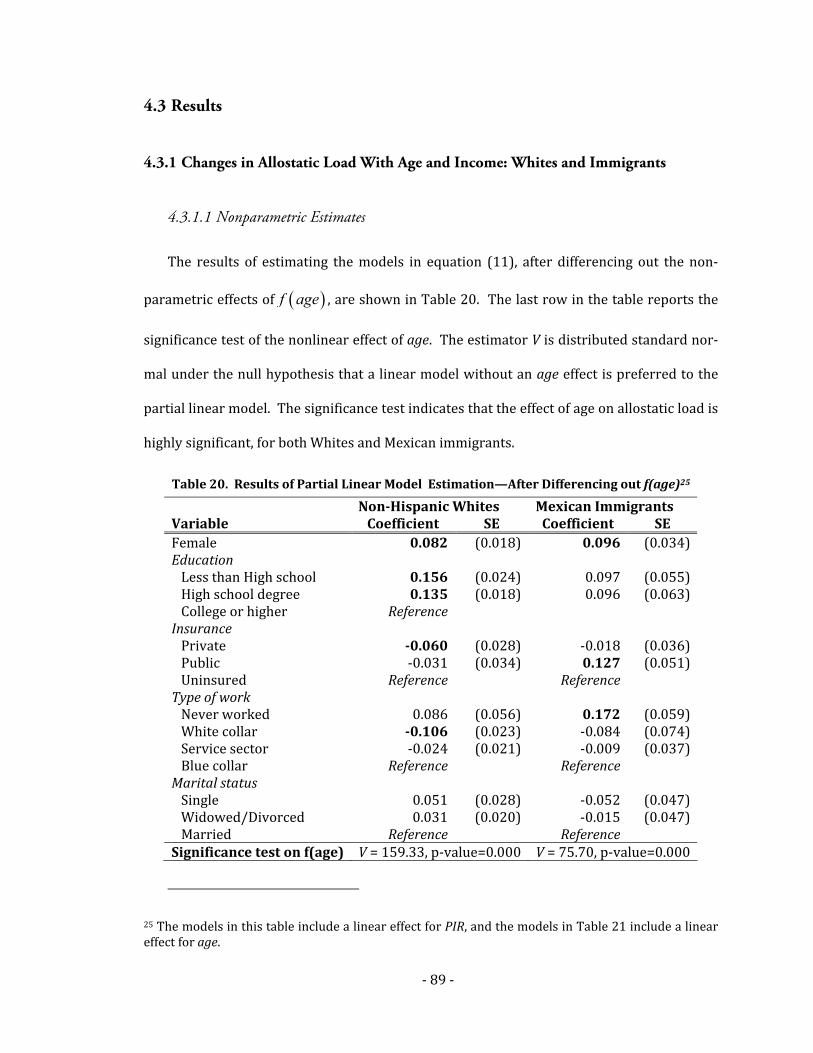
  ‐ 89 ‐ 

4.3 Results

4.3.1 Changes in Allostatic Load With Age and Income: Whites and Immigrants

4.3.1.1 Nonparametric Estimates

The  results  of  estimating  the models  in  equation  (11),  after  differencing  out  the non‐

parametric effects of f age , are shown in Table 20.  The last row in the table reports the 

significance test of the nonlinear effect of age.  The estimator V is distributed standard nor‐

mal under the null hypothesis that a linear model without an age effect is preferred to the 

partial linear model.  The significance test indicates that the effect of age on allostatic load is 

highly significant, for both Whites and Mexican immigrants. 

Table 20.  Results of Partial Linear Model  Estimation—After Differencing out f(age)25 

  Non­Hispanic Whites  Mexican Immigrants Variable  Coefficient  SE  Coefficient  SE Female  0.082  (0.018) 0.096  (0.034)Education      Less than High school  0.156  (0.024) 0.097  (0.055)   High school degree  0.135  (0.018) 0.096  (0.063)   College or higher  Reference  Insurance      Private  ­0.060  (0.028) ‐0.018  (0.036)   Public  ‐0.031 (0.034) 0.127  (0.051)   Uninsured  Reference Reference Type of work      Never worked  0.086 (0.056) 0.172  (0.059)   White collar  ­0.106  (0.023) ‐0.084  (0.074)   Service sector  ‐0.024 (0.021) ‐0.009  (0.037)   Blue collar  Reference Reference Marital status      Single  0.051 (0.028) ‐0.052  (0.047)   Widowed/Divorced  0.031 (0.020) ‐0.015  (0.047)   Married  Reference Reference Significance test on f(age)  V = 159.33, p‐value=0.000 V = 75.70, p‐value=0.000

                                                             

25 The models in this table include a linear effect for PIR, and the models in Table 21 include a linear effect for age. 

 

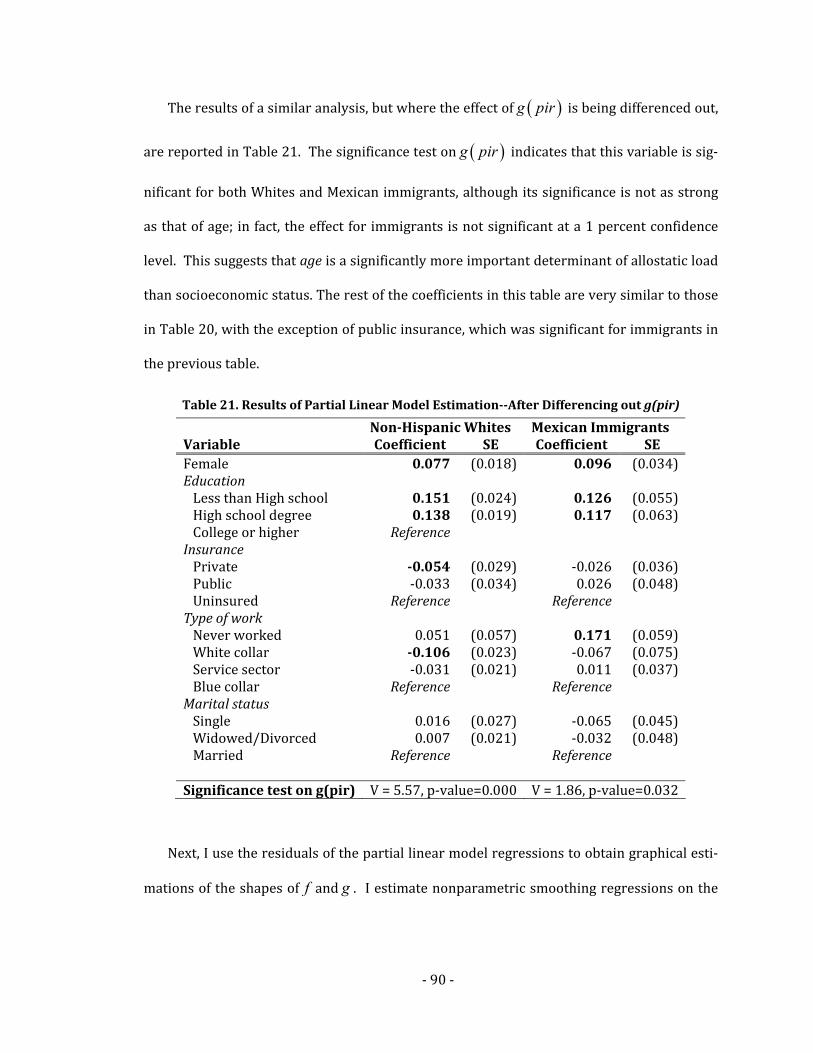
  ‐ 90 ‐ 

The results of a similar analysis, but where the effect of g pir  is being differenced out, 

are reported in Table 21.  The significance test on g pir  indicates that this variable is sig‐

nificant for both Whites and Mexican immigrants, although its significance is not as strong 

as that of age;  in fact, the effect for immigrants is not significant at a 1 percent confidence 

level.  This suggests that age is a significantly more important determinant of allostatic load 

than socioeconomic status. The rest of the coefficients in this table are very similar to those 

in Table 20, with the exception of public insurance, which was significant for immigrants in 

the previous table. 

Table 21. Results of Partial Linear Model Estimation­­After Differencing out g(pir) 

  Non­Hispanic Whites  Mexican Immigrants Variable  Coefficient  SE  Coefficient  SE Female  0.077  (0.018) 0.096  (0.034)Education      Less than High school  0.151  (0.024) 0.126  (0.055)   High school degree  0.138  (0.019) 0.117  (0.063)   College or higher  Reference  Insurance      Private  ­0.054  (0.029) ‐0.026  (0.036)   Public  ‐0.033 (0.034) 0.026  (0.048)   Uninsured  Reference Reference Type of work      Never worked  0.051 (0.057) 0.171  (0.059)   White collar  ­0.106  (0.023) ‐0.067  (0.075)   Service sector  ‐0.031 (0.021) 0.011  (0.037)   Blue collar  Reference Reference Marital status      Single  0.016 (0.027) ‐0.065  (0.045)   Widowed/Divorced  0.007 (0.021) ‐0.032  (0.048)   Married  Reference Reference    Significance test on g(pir)  V = 5.57, p‐value=0.000 V = 1.86, p‐value=0.032

 

Next, I use the residuals of the partial linear model regressions to obtain graphical esti‐

mations of the shapes of f and g .   I estimate nonparametric smoothing regressions on the 

 

  ‐ 91 ‐ 

residuals.  The results of the nonparametric smoothing are shown in Figure 5.26  The graph 

on the upper left suggests that the shape of the allostatic load relationship with age is very 

similar  for Whites  and Mexican  immigrants,  although  immigrants  appear  to  have  a  slight 

health advantage at younger ages that gradually disappears, such that between ages 45 and 

55 the allostatic load scores of both groups are nearly identical.  At older ages, Whites have 

a growing health advantage over Mexican immigrants.  However, when we examine the 90 

percent confidence intervals of these lines, shown in the upper right graph, it appears that 

these differences are not large enough to be significant, with the possible exception of ages 

younger than 40, where there are some segments in which the confidence intervals do not 

overlap.  In terms of candidate functional forms to test for age, the shape of these lines sug‐

gest either a quadratic, cubic, or logarithmic form. 

Figure 5’s bottom row shows the estimated nonparametric regression lines for PIR.   A 

striking feature of this graph are the entirely different Health­SES trajectories of Whites and 

Mexican  immigrants.   At  low PIR values,  the  line  for Whites  starts  at  a  relatively high  al‐

lostatic  load  level  and  then decreases monotonically  as PIR  increases until  a PIR value of 

about three, after which it increases slightly.  On the other hand, the line for Mexicans at a 

PIR value of zero is about 0.25 AL units below the line for Whites, remains nearly flat as PIR 

increases until PIR levels close to two, and then increases slightly after that.   An examina‐

tion of the confidence intervals shows that, although the intervals overlap at high PIR levels, 

there are significant differences at PIR  levels below 1.5.   At  first sight,  it  is not clear what 

functional forms can be tested for PIR, but it is possible that a cubic form can approximate 

these shapes.   

                                                             

26 I use a version of plreg—modified with permission from its author, Michael Lokshin—that allows for the estimation of confidence intervals. 

 

  ‐ 92 ‐ 

Regardless of the appropriate functional form, the AL­PIR graph suggests two significant 

results.  First, income is associated more strongly with health status for Whites than it is for 

Mexican  immigrants.    It  is not difficult  to notice  that  the PIR  line  for  immigrants  is nearly 

flat, while the line for Whites has a clear negative slope from low income up until PIR values 

near three.  Second, not only is the relationship between AL and SES weak, but it could even 

be  positive,  such  that  higher  income  levels  are  associated  with  somewhat  worse  health 

status.    Given  the widely  acknowledged  strong  and  negative  relationship  between  health 

and socioeconomic status, if confirmed, this is an important finding, and it is consistent with 

previous  findings  of  weak  Health­SES  gradients  among  Hispanics  in  the  United  States 

(Goldman  et  al.  2006;  Turra  and  Goldman  2007)  and  of  a  positive  Health­SES  gradient 

among Mexican Americans (Zsembik and Fennell 2005).   

It is important to note, however, that other confounding factors not taken into account 

in the previous analyses may produce the observed patterns, even if the Health­SES gradient 

is  strong  and  negative  for  Mexican  immigrants.    Below,  I  examine  whether  immigrants’ 

length of residence  in the United States could be a  factor explaining these Health­SES pat­

terns, and I evaluate whether other evidence supports some of the potential hypotheses to 

explain the apparent faster decline in health among Mexican immigrants. 

 

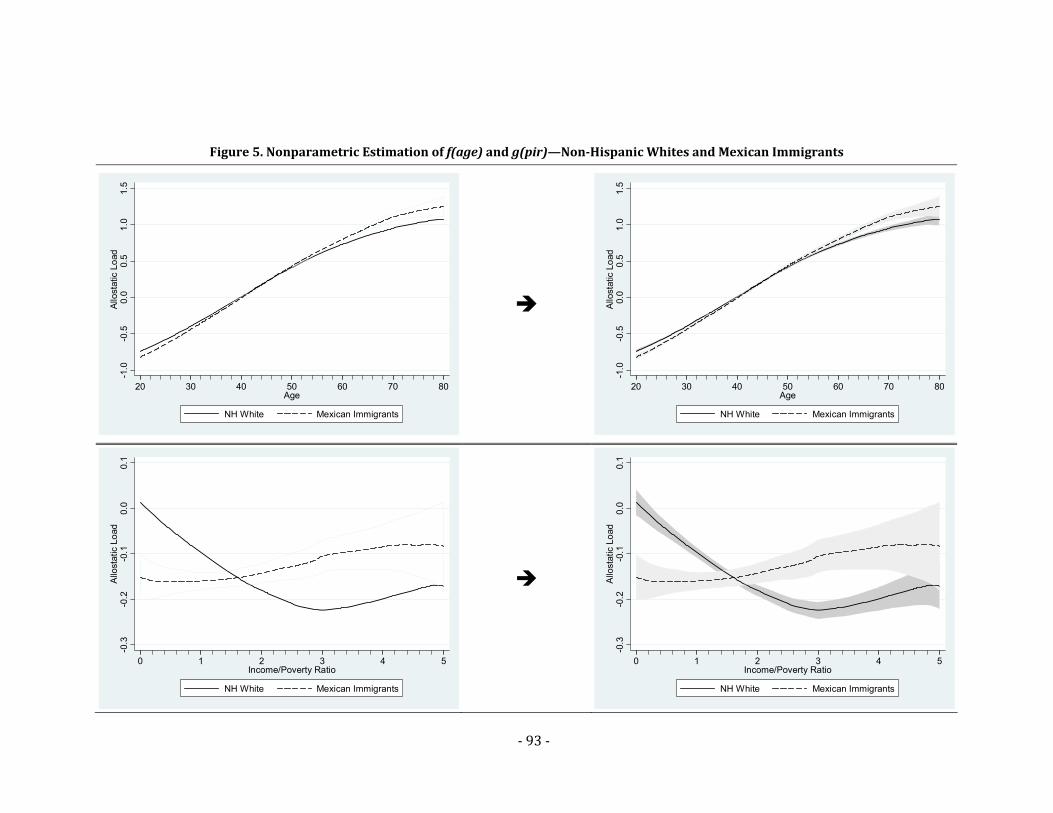
  ‐ 93 ‐ 

Figure 5. Nonparametric Estimation of f(age) and g(pir)—Non­Hispanic Whites and Mexican Immigrants 

-1.0

-0.5

0.0

0.5

1.0

1.5

Allo

stat

ic L

oad

20 30 40 50 60 70 80Age

NH White Mexican Immigrants

 

 

-1.0

-0.5

0.0

0.5

1.0

1.5

Allo

stat

ic L

oad

20 30 40 50 60 70 80Age

NH White Mexican Immigrants

 

-0.3

-0.2

-0.1

0.0

0.1

Allo

stat

ic L

oad

0 1 2 3 4 5Income/Poverty Ratio

NH White Mexican Immigrants

 

 

-0.3

-0.2

-0.1

0.0

0.1

Allo

stat

ic L

oad

0 1 2 3 4 5Income/Poverty Ratio

NH White Mexican Immigrants

 

  ‐ 94 ‐ 

4.3.1.2 Parametric Estimates

I estimate the following regression models, some of them suggested by the nonparamet‐

ric regressions in Figure 5, and others to avoid the potential of missing a better specification 

than those suggested by the graphs:  

 

1

21 2

2 31 2 3

1

1.

2.

3.

4. log .

AL z x

AL z x x

AL z x x x

AL z x

  (12) 

Where  ,x age pir , and the other terms are the same as defined above.  The signifi‐

cance test for each of these functional forms is conducted using the mean square residuals 

of the partial linear models in (11) and the parametric models in (12).  The test statistic is: 

 

2 2

20,1 .

dres diff

diff

s sV m n N

s

  (13) 

Where m  is  the order of differencing used to estimate the partial  linear model (higher 

orders are more efficient, plreg can estimate up to 10th‐order differencing); n is the sample 

size  before  differencing;  2ress   is  the  mean  square  residual  of  the  parametric  model;  and 

2diffs is the mean square residual of the partial linear model.  Under the null hypothesis that 

the parametric model is correct, V is distributed standard normal. 

The results of the significance tests for all models in (12) are reported in Table 22.  The 

estimated p‐values indicate that, at a significance level of 5 percent, none of the parametric 

models  adequately  capture  the  relationships  allostatic  load‐age  and  allostatic  load‐PIR.  

Nevertheless, the cubic form of age (both Whites and Mexican immigrants), and the quad‐

ratic form of PIR (Mexican immigrants) are satisfactory at a significance level of 1 percent.  

 

  ‐ 95 ‐ 

On the other hand, none of the four parametric specifications are adequate for  g PIR  for 

Whites, since their specification tests are highly significant.  This function probably requires 

a more complex specification than those I explore in this chapter.    I conclude that none of 

these parametric forms adequately approximate the functional form of  g PIR  for Whites, 

and  that  f age   for both groups and  g pir   for Mexican  immigrants  can be  somewhat 

reasonably approximated by cubic and quadratic forms, respectively.   

Table 22. Specification Tests of Parametric Models—Non­Hispanic Whites 

Parametric Model Parametric Mean Square Residual 

PLM Mean Square Residual 

V  p­value  Best 

Whites               Age linear  0.5925  8.09  0.000       Age quadratic  0.5838  3.17  0.001       Age cubic  0.5818  2.04  0.021       Age logarithmic  0.5869 

0.5782 

4.93  0.000       PIR linear  0.5925  5.39  0.000       PIR quadratic  0.5924  5.33  0.000       PIR cubic  0.5924  5.33  0.000       PIR logarithmic  0.5919 

0.5829 

5.05  0.000              Mexican  Immigrants 

         

    Age linear  0.5798  4.00  0.000       Age quadratic  0.5737  2.21  0.014       Age cubic  0.5720  1.71  0.044       Age logarithmic  0.5770 

0.5662 

3.18  0.001       PIR linear  0.5798  2.41  0.008       PIR quadratic  0.5799  2.01  0.022       PIR cubic  0.5801  2.06  0.020       PIR logarithmic  0.5820 

0.5730 

2.62  0.004            

 

 

  ‐ 96 ‐ 

4.3.2 Evidence For and Against Hypotheses of Changes in Immigrant Health Over

Length of US Residence

4.3.2.1 Immigrant Health Selection

The semiparametric estimation of the allostatic load‐age and ‐SES trajectories for recent 

immigrants  is  shown  in  Figure  6.    Three  important  conclusions  can  be  derived  from  this 

figure:  (1)  there  is  clear evidence of health selection: most  recent  immigrants have  lower 

levels of allostatic load than Whites of similar age and socioeconomic status; (2) this selec‐

tion appears to be limited to young and middle‐aged immigrants, since those of age 60 and 

older are increasingly less healthy than Whites; and (3) the striking result found in section 

4.3.1,  that  the AL­SES  relationship  is  weaker  for  immigrants  than  for Whites,  disappears 

once we  limit  the comparison to recent  immigrants; not only  is  the shape of  this relation‐

ship  similar,  with  the  exception  of  an  inverse  “hump”  at mid‐income  levels,  but  also  the 

strength of the association is similar for immigrants and Whites, and perhaps even stronger 

for immigrants.  As expected, the standard errors of these plots are larger than before, but 

they are sufficiently small at young ages and low income levels to be confident about these 

conclusions. 

The  results  in  this  figure  highlight  the  importance  of  taking  into  account  factors  that 

may have a significant role in mediating relationships such as that of allostatic load and age, 

or allostatic  load and SES.   While  from Figure 5 we could have concluded that  the AL‐SES 

relationship  is weak and perhaps positive  for  immigrants,  the graphs  in Figure 6  indicate 

that that is not the case, at least for recent immigrants. 

 

  ‐ 97 ‐ 

Figure 6. Allostatic Load Age and SES Trajectories—Recent Immigrants vs. Non­Hispanic Whites 

-1.0

0.0

1.0

2.0

Allo

stat

ic L

oad

20 30 40 50 60 70 80Age

NH White Mexican Immigrants

Years Since Immigration: <5

 

 

-1.0

0.0

1.0

2.0

Allo

stat

ic L

oad

20 30 40 50 60 70 80Age

NH White Mexican Immigrants

Years Since Immigration: <5

 

-0.8

-0.6

-0.4

-0.2

0.0

Allo

stat

ic L

oad

0 1 2 3 4 5Income/Poverty Ratio

NH White Mexican Immigrants

Years Since Immigration: <5

 

 

-0.8

-0.6

-0.4

-0.2

0.0

Allo

stat

ic L

oad

0 1 2 3 4 5Income/Poverty Ratio

NH White Mexican Immigrants

Years Since Immigration: <5

 

  ‐ 98 ‐ 

4.3.2.2 Immigrant Health-Age and Health-SES Trajectories by Length of US Residence

Comparisons  of  the  estimated  f   and  g   functions  for  different  immigrant  groups—

categorized by their length of US residence—are shown in Figure 7.  Because there were too 

few observations at older ages, which resulted in extremely large confidence intervals that 

limited  the  usefulness  of  the  graph  because  of  the  scale  of  the  y‐axis,  I  restricted  these 

graphs to individuals of age 78 or younger.     The fitted lines in the top panel indicate that 

young  and middle‐aged  recent  immigrants  are  healthier  than  immigrants  of  similar  ages 

who arrived to the US more five or more years earlier.  In particular, for immigrants between 

roughly 32 and 54 years of age, the estimated differences are large enough to be outside the 

area of overlap of the 90 percent confidence intervals.   At ages over 70, recent  immigrants 

appear to be less healthy than the other two immigrant groups, although there is consider‐

able overlap of  the confidence  interval at all ages over 60.   Worse health status of elderly 

recent immigrants is consistent with the negative selection at older ages found above. 

With respect  to  the AL­SES  trajectories,  the picture  is even clearer:  recent  immigrants 

are healthier than earlier immigrants of similar income levels across the entire range of in‐

come/poverty ratios reported in NHANES.  Moreover, we now see that not only recent  im‐

migrants, but also immigrants with over 15 years of residence in the US, have a negative and 

similarly strong relationship with PIR.   The only group with a weaker AL­SES relationship, 

and that resembles the plot shown in Figure 5, are immigrants with a US residence length 

between 5 and 15 years.  Therefore, the weak Health­SES patterns found above appear not 

to be an intrinsic trait of Mexican immigrants, but rather a result of the initial health selec‐

tivity  of migration  and  an  apparent  decline  in health over  the  length of  immigrants’  resi‐

dence in the United States. 

 

  ‐ 99 ‐ 

Figure 7. Allostatic Load­Age and ­SES Trajectories­­By Length of US Residence -1

.00.

01.

02.

0A

llost

atic

Lo

ad

20 30 40 50 60 70 80Age

15+ yrs 5-15 yrs< 5 yrs

 

 

-1.0

0.0

1.0

2.0

Allo

stat

ic L

oad

20 30 40 50 60 70 80Age

15+ yrs 5-15 yrs< 5 yrs

 

-1.0

0-0

.50

0.00

0.50

1.00

Allo

stat

ic L

oad

0 1 2 3 4 5Income/Poverty Ratio

15+ yrs 5-15 yrs< 5 yrs

 

 

-1.0

0-0

.50

0.00

0.50

1.00

Allo

stat

ic L

oad

0 1 2 3 4 5Income/Poverty Ratio

15+ yrs 5-15 yrs< 5 yrs

 

  ‐ 100 ‐

4.3.2.3 Comparing Immigrant Cohorts: NHANES-III vs. 2001-2004 NHANES

One potential explanation for the apparent decline in immigrant health as the length of 

residence  in  the United  States  increases  does  not  involve  a  health  decline  over  time,  but 

rather the possibility that recent immigrant arrival cohorts are healthier than earlier arrival 

cohorts.  This would explain both the Health­SES patterns found in Figure 5, because earlier 

arrival cohorts would have higher SES levels due to having lived in the US longer and would 

be  less  healthy due  to  the  hypothesized  cohort  differences,  as well  as  the  differences  be‐

tween immigrants according to the length of their US residence found in Figure 7.   

The available information on time since arrival to the US in the 1999‐2004 NHANES se‐

verely  limits my ability  to construct accurate arrival  cohorts.   Thus,  I  can only define  two 

arrival cohorts: those who were recent arrivals during in NHANES‐III, and those who were 

recent arrivals in the 1999‐2004 NHANES.  The estimated  f  and  g  functions for these two 

immigrant arrival cohorts are shown in Figure 8.  In this case, recent immigrants are defined 

as those having arrived within 10 years of the survey.  I change the definition of recent im‐

migrant in order to maintain a reasonable sample size and yet, the standard errors are high 

at older ages and high income levels.   Nevertheless, the plots at young and middle ages, and 

at  low  and  middle  income  levels,  suggest  that  there  are  no  significant  differences  in  al‐

lostatic load scores between these two arrival cohorts.  Furthermore, if there are any differ‐

ences,  the more  recent  immigrant  cohort  appears  to  be  less  healthy  than  the  1988‐1994 

immigrant  cohort,  exactly  the opposite of what we would expect  if  cohort effects were  to 

explain the patterns found in Figure 7.   These results are consistent with those of Antecol 

and Bedard (2006), who did not  find significant health differences between several  immi‐

grant arrival cohorts (1980 and before, 1981‐1985, 1986‐1990, and 1991‐1996) 

 

  ‐ 101 ‐

4.3.2.4 Acculturation Effects—Spanish- vs. English-Speaking Immigrants

Finally, to assess whether there is any indication that health declines with acculturation, 

I restrict the sample to immigrants who have lived in the United States for 10 years or longer 

and I stratify the semiparametric analyses by the language spoken at home.  The results are 

shown in Figure 9.   There is no indication that Spanish‐speaking immigrants are healthier 

than  English‐speaking  immigrants.    In  fact,  Spanish  speakers  have  higher  allostatic  load 

values  than English  speakers over nearly  the entire  age  range,  although  these differences 

are  generally  not  large  enough  to  be  outside  the  confidence  intervals.    One  limitation  of 

these  analyses  is  that  they do not  account  for  the possibility  that English‐speaking  immi‐

grants were  healthier  than  Spanish‐speaking  immigrants  at  the  time  of  arrival  to  the US.  

Unfortunately, I cannot test for this possibility because the sample size of recent immigrants 

who speak English is too small (less than 5 percent of the sample of recent Mexican immi‐

grants).  In fact, this can be considered as an argument for the validity of these analyses: 10 

years after arrival, nearly 32 percent of the sample speak at least some English, which indi‐

cates that over 25 percent of  immigrants have acculturated to some extent, and the accul‐

turated are healthier than the unacculturated. 

Nevertheless,  as  discussed  above,  acculturation  is  multi‐dimensional  and  language  is 

only one of  its many components.   Therefore,  it may still be the case that acculturation  in 

other dimensions may have negative health consequences. Results using other measures of 

acculturation  such  as  diet,  cultural  beliefs,  or  civic  participation  could  be  different  from 

those found here.   Nevertheless,  language spoken at home remains a valid indicator of ac‐

culturation, and  the results reported  in Figure 9 do suggest  that more acculturated  immi‐

grants are healthier than the less acculturated. 

 

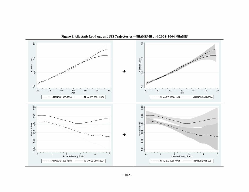
  ‐ 102 ‐

Figure 8. Allostatic Load Age and SES Trajectories—NHANES­III and 2001­2004 NHANES  -1

.00.

01.

02.

0A

llost

atic

Lo

ad

20 30 40 50 60 70 80Age

NHANES 1988-1994 NHANES 2001-2004

 

 

-1.0

0.0

1.0

2.0

Allo

stat

ic L

oad

20 30 40 50 60 70 80Age

NHANES 1988-1994 NHANES 2001-2004

 

-1.0

0-0

.80

-0.6

0-0

.40

-0.2

00.

00A

llost

atic

Lo

ad

0 1 2 3 4 5Income/Poverty Ratio

NHANES 1988-1994 NHANES 2001-2004

 

 

-1.0

0-0

.80

-0.6

0-0

.40

-0.2

00.

00A

llost

atic

Lo

ad

0 1 2 3 4 5Income/Poverty Ratio

NHANES 1988-1994 NHANES 2001-2004

 

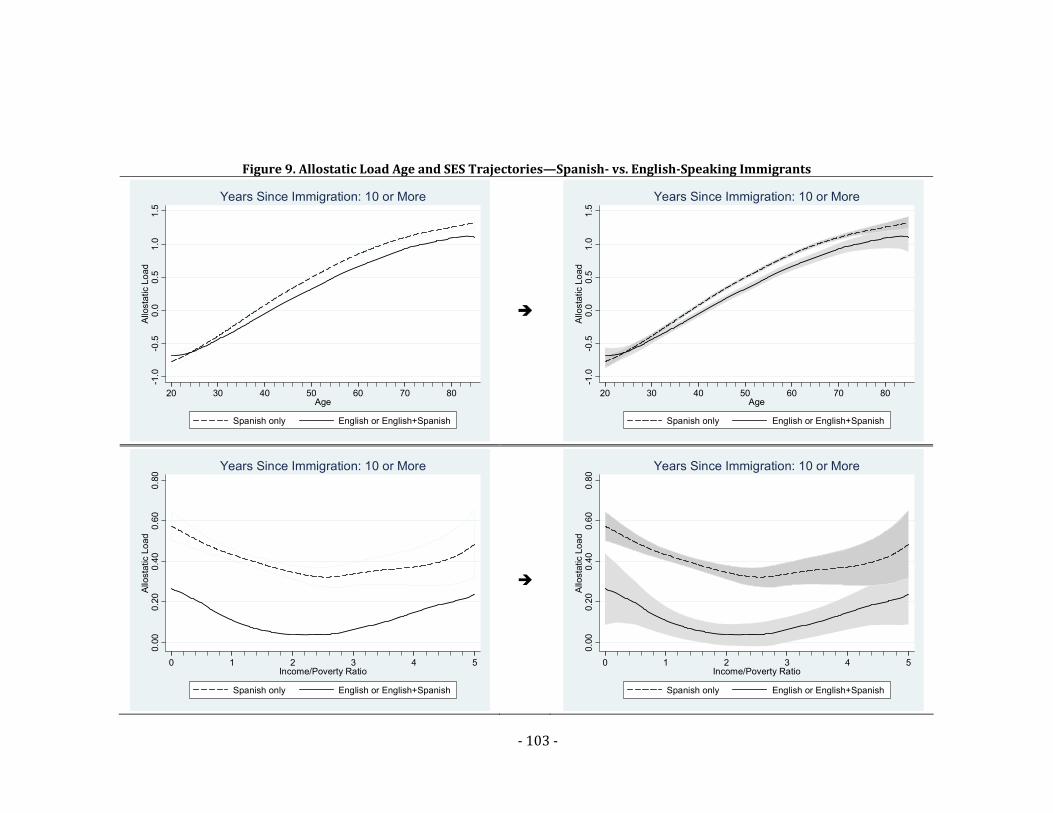
  ‐ 103 ‐

 Figure 9. Allostatic Load Age and SES Trajectories—Spanish­ vs. English­Speaking Immigrants 

-1.0

-0.5

0.0

0.5

1.0

1.5

Allo

stat

ic L

oad

20 30 40 50 60 70 80Age

Spanish only English or English+Spanish

Years Since Immigration: 10 or More

 

 

-1.0

-0.5

0.0

0.5

1.0

1.5

Allo

stat

ic L

oad

20 30 40 50 60 70 80Age

Spanish only English or English+Spanish

Years Since Immigration: 10 or More

 

0.00

0.20

0.40

0.60

0.80

Allo

stat

ic L

oad

0 1 2 3 4 5Income/Poverty Ratio

Spanish only English or English+Spanish

Years Since Immigration: 10 or More

 

 0.

000.

200.

400.

600.

80A

llost

atic

Lo

ad

0 1 2 3 4 5Income/Poverty Ratio

Spanish only English or English+Spanish

Years Since Immigration: 10 or More

 

  ‐ 104 ‐

4.4 Conclusion

The analyses in this chapter support some of the hypotheses that are common in the lit‐

erature on immigrant health, but raise some doubts about others.  First, the semiparametric  

analyses  I  conduct  on  the  full  sample  of Mexican  immigrants  indicate  that  (1)  immigrant 

health declines relative  to that of US‐born Whites as the  length of US residence  increases; 

and (2) the Health­SES gradient of immigrants is flatter than that of Whites, and it might be 

slightly positive at higher income levels.  

However, when I divide the sample of Mexican immigrants according to length of resi‐

dence in the United States, the health patterns are somewhat different from those described 

above.   More specifically, a comparison of recent Mexican immigrants with Whites suggest 

that immigrants are indeed positively selected on health status, because their allostatic load 

levels are lower than those of Whites at ages below 60. On the other hand, the health selec‐

tivity of older Mexican immigrants appears to be negative, which is consistent with younger 

Mexicans  being  likely  to  migrate  for  economic  reasons,  but  older  Mexicans  being  more 

likely to migrate to reunite with their family.   These comparisons also reveal a Health­SES 

gradient for recent immigrants similar to that of Whites, suggesting that the weak gradient 

found in other studies is an artifact of health changes over immigrants’ life course.  

Indeed, when the allostatic load patterns of recent immigrants are compared to the pat‐

terns of immigrants with 5‐15 years of residence in the US, and to those of immigrants with 

over 15 years of US residence, the results show a better health status for the former group 

compared to the latter two.  This is consistent with the result, often found in the literature, 

that immigrant health decreases with length of residence in the United States.  However, it 

is  important  to note  that  this does not necessarily  imply  that  immigrant health decreases 

 

  ‐ 105 ‐

with acculturation since, as discussed above, increased length of residence is not necessarily 

a good indicator of acculturation. 

One potential hypothesis  to explain  the worsening of  immigrant health with  length of 

residence in the United States is the existence of health differences between different immi‐

grant  cohorts.    However, when  I  test  this  hypothesis  by  comparing  recent  immigrants  in 

NHANES‐III  with  recent  immigrants  in  the  2001‐2004  NHANES,  I  do  not  find  significant 

differences between both cohorts.   If anything, the results suggest that the NHANES‐III co‐

hort of recent immigrants might have been healthier than its counterpart in the 2001‐2004 

NHANES,  contrary  to  the hypothesis  that would explain  the results described above.   The 

confidence intervals are too wide in this analysis, though; thus, larger sample sizes are re‐

quired to draw any definitive conclusions. 

Finally, I try to identify acculturation effects on immigrant health by comparing the al‐

lostatic load patterns of Mexican immigrants who have lived in the US for at least ten years 

and who speak only Spanish at home, with those of immigrants with at least ten years of US 

residence, but who speak at least some English at home.   The results indicate opposite re‐

sults  to  those  expected  under  the  acculturation  hypothesis:  more  acculturated  (English 

speaking) immigrants are healthier than less acculturated immigrants.  Although the differ‐

ences are not always outside the 90 percent confidence intervals, they are large enough to 

be statistically significant between ages 40 and 70, and at most PIR levels below 3.5. 

Overall,  the analyses  in  this chapter do not support  the hypothesis of acculturation or 

healthier recent cohorts, suggesting that either the life­course hypothesis or the regression to 

the mean hypothesis are more  likely  to be correct.   That  is,  the observed decline  in  immi‐

grant health with increases in length of US residence may be due to either (a) the cumula‐

tive effect of the hardships migrants experience over their lifetime, or (b) a convergence of 

immigrant health status to the average health levels in their home countries. 

 

  ‐ 106 ‐

An important contribution of this analysis is the insight it provides into what Goldman 

and colleagues (2006) have called a “second Hispanic Paradox”: the apparent weak or even 

flat Health­SES  gradient  among Hispanics  living  in  the United  States.   My  results  indicate 

that  the Health­SES  gradient  among Mexican  immigrants  is  indeed negative  and  about  as 

steep as that of non‐Hispanic Whites.   The weak gradient that  is observed when all  immi‐

grants are examined together is an artifact of the decline in immigrant health with length of 

US  residence:  as  immigrants’  duration  of  residence  increases,  so  does  their  income,  but 

given the decline in health associated with longer stay in the US, we observe better health 

among low‐income immigrants (who are more likely to be recent immigrants) than among 

high‐income immigrants (who are likely to have lived for more years in the US).  As Figure 7 

suggests,  when  immigrants  are  divided  according  to  their  length  of  US  residence,  their 

Health­SES gradients resemble those of US‐born Whites (the exception appears to be immi‐

grants with a residence between 5 and 15 years.)  I should note, however, that several of the 

studies that found a weak gradient among Hispanics used education as the measure of SES 

instead of income.  In this study I focused on income because it is a continuous variable that 

allows me to conduct semiparametric analyses that I consider provide a greater insight into 

the nature of the Health‐SES relationship.  Nevertheless, future studies can explore the gra‐

dient while  stratifying  the  sample  by  length  of  US  residence,  in  order  to  verify  if  results 

similar to mine are obtained. 

 

 

  ‐ 107 ‐

Chapter 5. Discussion

This  work  sought  to  provide  a  better  understanding  of  the  issues  surrounding  the 

health of Hispanics in general and Hispanic immigrants in particular.  A first contribution of 

this study  is  the creation of an objective measure of biological risk that weighs each of  its 

components according to their association with mortality, and takes into account potential 

nonlinearities in those associations.  A second contribution is my emphasis on the potential 

usefulness of semiparametric methods in the study of health disparities.    I apply two such 

methods in my analysis: First, I use propensity score estimators to estimate the health gap 

between  Whites,  US‐born  Mexicans,  and  Mexican  immigrants.    Second,  I  use  a  semi‐

parametric  differencing  estimator  combined  with  nonparametric  smoothing  in  order  to 

analyze  the  health  patterns  of Mexican  immigrants,  and  how  they  compare  to  the  health 

patterns of Whites.   Below,  I summarize my main  findings and discuss  the  implications of 

this research. 

5.1 Main Findings

In Chapter 3,  I examined the existence of a health advantage of  individuals of Mexican 

ethnicity over non‐Hispanic Whites  in the United States, a phenomenon commonly known 

as the “Hispanic Paradox.”  My main results indicate that this paradox is a phenomenon re‐

lated to  immigration.   When I use allostatic  load to compare health status between ethnic 

groups, US‐born Mexicans are found to be less healthy than both Whites and Mexican immi‐

grants.   This health disadvantage  exists not only  for  the  summary  index of  allostatic  load 

(AL), but also for each of its three subcomponents (inflammatory, metabolic, and cardiovas‐

cular).    Mexican  immigrants  have  lower  (i.e.,  better)  allostatic  load  scores  than  US‐born 

Mexicans,  and  lower  inflammatory  and  cardiovascular  scores  than Whites.   However,  the 

 

  ‐ 108 ‐

metabolic scores of Mexican immigrants are higher than those of Whites, and so the overall 

allostatic load score is not significantly different between Whites and immigrants. 

On the other hand, similar analyses that use the 10‐year risk of coronary heart disease 

as the outcome, estimated using the Framingham scoring system (FRS), produce somewhat 

different results.  In this case, both US‐born Mexicans and Mexican immigrants are found to 

have  lower  risk of  coronary heard disease  (CHD)  than Whites, which  is  consistent with  a 

general Hispanic Paradox.   I attempt to reconcile the FRS and AL results by first removing 

from the Framingham score  the risk  factors not  included  in  the AL measure, and  then re‐

moving  from  allostatic  load  the  biomarkers  not  included  in  the  Framingham  score.    Al‐

though some differences persist when I use these  ‘reduced’ measures, the FRS models are 

generally consistent with  the AL models  regarding  the health of Mexican  immigrants  (i.e., 

Mexican immigrants enjoy health similar to Whites, although they have advantages in some 

areas  and  disadvantages  in  others).    Regarding  US‐born Mexicans,  I  find  the  evidence  as 

convincingly suggesting that they are less healthy than Whites. 

In  Chapter  4,  I  explore  the Health­age  and Health­SES  trajectories  of  Mexican  immi‐

grants.    I use semiparametric methods to estimate  these  trajectories over  the  full age and 

SES  range  available  in  NHANES.   Moreover,  I  assess  the  evidence  supporting  several  hy‐

potheses that have been presented in the literature on immigrant health.  Consistently with 

results in other research, I find indirect evidence supporting the positive health selection of 

Mexican migrants and a decline in immigrant health with increases in duration of residence 

in the United States.  However, unlike other studies, I find that the Health­SES gradients are 

similar for Whites, recent immigrants, and immigrants who have lived in the US more than 

15 years.  Only immigrants with 5‐15 years of residence appear to have a weaker gradient 

when compared  to US‐born Whites.    In addition,  I do not  find support  for  the hypotheses 

that  immigrant  health  worsens  with  acculturation,  or  that  recent  immigrant  cohorts  are 

 

  ‐ 109 ‐

healthier  than earlier  immigrant  cohorts.   Overall,  the  results  in  this  chapter  suggest  that 

the  observed  decline  in  immigrant  health with  increases  in  duration  of  US  residence  are 

more likely to be due to either (a) the cumulative negative effect of the adversities associ‐

ated with the process of migration, or (b) a regression of  immigrant health to the average 

health levels in their countries of origin. 

5.2 Future Research and Policy Implications

An important first implication of the analyses in Chapter 3 is that researchers need to be 

cautious when using self‐assessments of health status or self‐reports of health conditions to 

compare the health of different ethnic groups.   As shown in Tables 2 and 3,  the results of 

those  analyses  are  ambiguous  and  largely  dependent  on  the measure  chosen.    Objective 

health measures that use biomarkers or other unbiased indicators of health should be used 

in these studies whenever possible.  

Further research  is needed to verify my result  that US‐born Mexicans are  less healthy 

than non‐Hispanic Whites and Mexican immigrants.  If confirmed, this is an important result 

with at  least three significant implications: (1) future analyses of ethnic disparities should 

divide the samples by country of birth, or should add country of birth interaction terms if 

the analyses are pooled across ethnic groups; (2) other studies need to assess whether this 

disadvantage  exists  not  only  for US‐born Mexicans,  but  also  for  other US‐born Hispanics; 

and (3) a focus of future research should be identifying the causes of this health disadvan‐

tage. 

With respect to Mexican immigrants, it is necessary to establish why positive health se‐

lection  of  migrants  does  not  translate  in  a  health  advantage  in  biomarkers  of  metabolic 

functioning.    Evidently,  the  processes  that  lead  to  better  health  status  of migrants  in  in‐

flammatory  and  cardiovascular  functioning do not produce  the  same  result  for metabolic 

 

  ‐ 110 ‐

indicators.  This is important not only from an academic perspective, but also because dia‐

betes  and obesity  are  increasingly  important health problems  for Hispanics  in  the United 

States and in countries like Mexico.  If the root causes of this disadvantage are cultural, both 

US and Mexican governments need to engage in public health campaigns to neutralize them 

before the diabetes and obesity epidemics grow even more in importance.  

Another important implication of this work is the lack of support for the acculturation 

hypothesis.   This  is a  theory that now has deep roots  in  the health  literature, so obviously 

further efforts are needed  to verify  these  findings using better measures of  acculturation.  

Nevertheless,  if  it  is  indeed the case  that acculturation does not necessarily  lead to worse 

health outcomes, researchers and policymakers need to become aware of it.  Moreover, my 

results suggest that acculturation—at least language acculturation—may actually be benefi‐

cial for health.   This could occur through better access to the healthcare system, increased 

health literacy, or simply through a feeling of belonging to US society.  All of these alterna‐

tives need to be explored because they could be of great importance to future policy efforts 

aimed towards immigrants. 

My results regarding the health trajectories of Mexican immigrants are consistent with 

two hypothesis: (1) the  life­course hypothesis, which states that the adversities associated 

with migration are the cause of the decline of  immigrants’ health with increased length of 

US residence, and  (2)  the regression  to  the mean  hypothesis, which states  that  this health 

decline is simply a result of a convergence of immigrant health to the health profiles in their 

country of origin.     The available data does not allow me to specifically test either of these 

two hypotheses against each other.  I am only aware of two studies that have attempted to 

test  for  regression  to  the mean  in  a  health  context.   Chiswick  et  al.  (2008)  found  that  the 

health  of  four  different  types  of  immigrants  declined  at  different  rates  over  a  three‐year 

period.   Since  three of  the  four  types had similar rates of good health status upon arrival, 

 

  ‐ 111 ‐

under reversion to the mean we would expect their health status to decline at similar rates, 

thus their results cast some doubt on the regression to the mean hypothesis.   The authors 

also conclude that the observed health declines may be caused by several factors associated 

to  initial  adjustment  to  a new country,  including  “the  stress of  immigration”  (i.e.,  the  life­

course hypothesis), but they never formally test this premise.  Biddle et al. (2007) also exam‐

ine the extent  to which the health of  immigrants  to Australia varies over  time.   They con‐

sider  cohorts  of  immigrants  from  three different  groups  of  countries  of  birth,  and  expect 

similar  rates  of  health  decline  among  the  three  groups  under  the  regression  to  the mean 

hypothesis,  but  instead  find differences  in health  decline between  these groups,  thus  con‐

cluding that declines in health are more likely to be affected by “culture and environment.” 

For example, a recent study found that Mexican immigrants in the US and Mexicans with a 

family member in the US are at a higher risk to have suicidal thoughts than Mexicans with 

no migration history and no migrant relatives (Borges et al. 2009).   This suggests that the 

process of migration places migrants and their families under additional stress, above and 

beyond the stress experienced by non‐migrant households, which is consistent with the life‐

course perspective.   

Future research should explicitly test these two hypotheses, especially since the poten‐

tial  policy  implications  under  each  of  them  are  considerably  different.    In  particular,  the 

regression to the mean hypothesis implies that the decline in immigrant health is expected 

as a result of natural biological processes, and thus policies should focus on identifying the 

health risks likely to result from the convergence of immigrant health to the health profiles 

in their countries of origin (e.g., could the high incidence of diabetes among Hispanics have 

been anticipated given the diabetes epidemic that has affected countries like Mexico?).  On 

the other hand,  if  declines  in  immigrant health  are produced by higher  cumulative  stress 

throughout  the  life  course,  policies  should  focus  on  identifying  the  sources  of  additional 

 

  ‐ 112 ‐

stress in order to mitigate their effects and reduce, for example, the higher risk of suicidal 

thoughts among Mexicans found by Borges et al. (2009).  A potential research approach to 

test  these  hypotheses  is  to  compare  the  health  trajectories  of  undocumented  immigrants 

with those of legal immigrants.   Since the former are more likely to undergo a difficult mi‐

gration  process,  under  the  life­course  hypothesis we would  expect  their  health  to  decline 

faster than for legal immigrants.   On the other hand, under regression to the mean there is 

no a priori reason to expect  that both groups would have different rates of health decline 

over time. 

Two final remarks are warranted regarding alternative theories of the causes of immi‐

grant health deterioration.  First, it is possible that differential use of—or lack of access to—

the healthcare system is a contributing factor to explain a faster health decline among im‐

migrants than among the native US population.  For example, immigrants might be healthier 

upon arrival to the US, but lack of access to healthcare services may result in worse health 

outcomes over time.   Research indicates that immigrants use less healthcare services than 

the native US population  (Goldman, Smith, and Sood 2006).   Although  this may be due  to 

positive health selection and younger age among immigrants, lower use of medical care may 

result  in worse health outcomes over  time.    In addition, even  if  immigrants  increase  their 

use  of  healthcare  services  as  they  acculturate,  prejudice  among  healthcare  providers  and 

imperfect communication between patients and providers may result in lower quality in the 

provision  of  healthcare  (Escarce  2005;  Balsa,  McGuire,  and  Meredith  2005).    Therefore, 

another item for future research is the role of differences in the use of healthcare services 

and in the quality of services received as contributors to the deterioration of health status 

among immigrants. 

Second,  contextual  factors  may  mediate  the  relationship  between  immigrant  health 

status and duration of residence in the receiving country.  A theory related to this perspec‐

 

  ‐ 113 ‐

tive  is  that of segmented assimilation (Portes and Zhou 1993).   This  theory maintains  that 

immigrants with low SES levels may have no choice but to assimilate into low‐SES areas in 

the United States, thus experiencing both the adversities and negative influences associated 

with these areas.  On the other hand, other immigrants, most likely those with high SES lev‐

els upon arrival, may be able to replicate the traditional model of acculturation and integra‐

tion  into  the  White  middle‐class.    In  addition,  under  a  third  pattern  of  assimilation, 

immigrants may preserve their most important cultural traits while at the same time they 

assimilate into mainstream society, thus enjoying the benefits associated with assimilation.   

Although this theory is usually posited in the context of socioeconomic outcomes, it has 

been mentioned recently as a potential framework to explain the trajectories of immigrant 

health  (Goldman  et  al.  2006).    Testing  this  theory,  Finch  et  al.  (2007)  hypothesize  that 

neighborhood disadvantage and acculturation moderate the relationship between place of 

birth  and  low  birth  weight,  such  that  (a)  immigrant  women  who  live  in  disadvantaged 

neighborhoods are more likely to give birth to low‐weight infants than similar women living 

in  more  advantaged  neighborhoods,  (b)  immigrant  women  who  live  in  unacculturated 

neighborhoods are less likely to give birth to low‐weight infants than similar women living 

in more acculturated neighborhoods, and (c) the association between neighborhood disad‐

vantage and  low birth weight  is  similar  for native women and  immigrant women, but  the 

relationship between neighborhood acculturation and low birth weight is opposite between 

both groups of women.  Their findings generally support these hypotheses, thus suggesting 

that contextual factors indeed influence the health outcomes of immigrants.  Whether these 

effects result in different health patterns than those observed in this study is another issue 

that needs to be explored in future research. 

 

  ‐ 115 ‐

Bibliography

Abraido‐Lanza, A. F., M. T. Chao, and K. R. Florez. 2005. Do healthy behaviors decline with greater acculturation? Implications  for the Latino mortality paradox. Social Science & Medicine 61 (6):1243‐1255. 

Abraido‐Lanza,  A.  F.,  B.  P.  Dohrenwend,  D.  S.  Ng‐Mak,  and  J.  B.  Turner.  1999.  The  Latino Mortality  Paradox:  A  Test  of  the  "Salmon  Bias"  and  Healthy Migrant  Hypotheses. American Journal of Public Health 89 (10):1543‐1548. 

Acevedo‐Garcia,  Doiores,  Mah‐J.  Soobader,  and  Lisa  F.  Berkman.  2007.  Low  birthweight among  US  Hispanic/Latino  subgroups:  The  effect  of  maternal  foreign‐born  status and education. Social Science & Medicine 65:2503‐2516. 

Albrecht,  S.  L.,  L.  L.  Clarke, M.  K. Miller,  and  F.  L.  Farmer.  1996.  Predictors  of  differential birth  outcomes  among  Hispanic  subgroups  in  the  United  States:  The  role  of maternal risk characteristics and medical care. Social Science Quarterly 77 (2):407‐433. 

Anderson, K. M., P. M. Odell, P. W. Wilson, and W. B. Kannel. 1991. Cardiovascular disease risk profiles. Am Heart J 121 (1 Pt 2):293‐8. 

Antecol,  Heather,  and  Kelly  Bedard.  2006.  Unhealthy  assimilation:  Why  do  immigrants converge to American health status levels? Demography 43 (2):337‐360. 

Balsa, A. I., T. G. McGuire, and L. S. Meredith. 2005. Testing for statistical discrimination in health care. Health Serv Res 40 (1):227‐52. 

Bang, Heejunt, and  James M. Robins. 2005. Doubly Robust Estimation  in Missing Data and Causal Inference Models. Biometrics 61:962‐972. 

Becerra,  J.  E.,  C.  J.  R.  Hogue,  H.  K.  Atrash,  and  N.  Perez.  1991.  Infant‐Mortality  among Hispanics  ‐  a  Portrait  of  Heterogeneity.  Jama­Journal  of  the  American  Medical Association 265 (2):217‐221. 

Biddle,  Nicholas,  Steven  Kennedy,  and  James  T.  McDonald.  2007.  Health  assimilation patterns amongst Australian immigrants. The Economic Record 83 (260):16‐230. 

Blundell,  Richard,  Lorraine  Dearden,  and  Barbara  Sianesi.  2005.  Evaluating  the  Effect  of Education  on  Earnings:  Models,  Methods  and  Results  from  the  National  Child Development  Survey.  Journal of  the Royal Statistical Society, Series A  168  (3):473‐512. 

Borges, Guilherme, Joshua Breslau, Maxwell Su, Matthew Miller, Maria Elena Medina‐Mora, and  Sergio  Aguilar‐Gaxiola.  2009.  Immigration  and  Suicidal  Behavior  Among Mexicans and Mexican Americans. American Journal of Public Health 99 (4):728‐733. 

Caliendo,  Marco.  2006. Microeconometric  Evaluation  of  Labour Market  Policies.  Vol.  568, Lecture Notes in Economics and Mathematical Systems. Berlin: Springer. 

 

  ‐ 116 ‐

Caliendo,  Marco,  and  Sabine  Kopeinig.  2008.  Some  Practical  Guidance  for  the Implementation  of  Propensity  Score  Matching.  Journal  of  Economic  Surveys  22 (1):31‐72. 

Cameron, A. C., and P. K. Trivedi. 2005. Microeconometrics. Methods and Applications. New York, NY: Cambridge University Press. 

Chiswick, B. R., Y. L. Lee, and P. W. Miller. 2008. Immigrant Selection Systems and Immigrant Health. Contemporary Economic Policy 26 (4):555‐578. 

Cho, Youngtae, W. Parker Frisbie, Robert A. Hummer, and Richard G. Rogers. 2004. Nativity, Duration  of  Residence,  and  the  Health  of  Hispanic  Adults  in  the  United  States. International Migration Review 38 (1):184‐211. 

CONAPO.  2008. Migration  and Health:  Latinos  in  the  United  States. Mexico,  D.F.:  Consejo Nacional de Población. 

Cooper, R., J. Cutler, P. Desvigne‐Nickens, S. P. Fortmann, L. Friedman, R. Havlik, G. Hogelin, J. Marler, P. McGovern, G. Morosco, L. Mosca, T. Pearson,  J. Stamler, D. Stryer, and T. Thom.  2000.  Trends  and  disparities  in  coronary  heart  disease,  stroke,  and  other cardiovascular diseases in the United States ‐ Findings of the National Conference on Cardiovascular Disease Prevention. Circulation 102 (25):3137‐3147. 

Crimmins,  Eileen  M.,  Jun  K.  Kim,  Dawn  E.  Alley,  Arun  Karlamangla,  and  Teresa  Seeman. 2007. Hispanic Paradox in Biological Risk Profiles. American Journal of Public Health 97 (7):1305‐1310. 

de Ruijter, W., R. G. Westendorp, W. J. Assendelft, W. P. den Elzen, A. J. de Craen, S. le Cessie, and  J.  Gussekloo.  2009.  Use  of  Framingham  risk  score  and  new  biomarkers  to predict  cardiovascular  mortality  in  older  people:  population  based  observational cohort study. BMJ 338:a3083. 

Diez Roux, A. V., R. Detrano, S. Jackson, D. R. Jacobs, Jr., P. J. Schreiner, S. Shea, and M. Szklo. 2005.  Acculturation  and  socioeconomic  position  as  predictors  of  coronary calcification in a multiethnic sample. Circulation 112 (11):1557‐65. 

Donders, A. Rogier T.  , Geert  J.M.G. van der Heijdenn, Theo Stijnen, and Karel G.M. Moons. 2006.  Review:  A  gentle  introduction  to  imputation  of  missing  values.  Journal  of Clinical Epidemiology 59:1087‐1091. 

Dubowitz, Tamara, Stephanie A. Smith‐Warner, Doiores Acevedo‐Garcia, S.V. Subramanian, and RD Karen E. Peterson, ScD. 2007. Nativity and Duration of Time  in  the United States:  Differences  in  Fruit  and  Vegetable  Intake  Among  Low‐Income  Postpartum Women. American Journal of Public Health 97 (10):1787‐1790. 

Elo,  I.  T.,  C. M.  Turra,  B.  Kestenbaum,  and  B.  R.  Ferguson.  2004. Mortality  among  elderly Hispanics  in  the  United  States:  Past  evidence  and  new  results.  Demography  41 (1):109‐128. 

Escarce, J. J. 2005. How does race matter, anyway? Health Services Research 40 (1):1‐7. 

 

  ‐ 117 ‐

Escarce,  Jose  J.,  Leo  S.  Morales,  and  R.  G.  Rumbaut.  2006.  The  health  status  and  health behaviors of Hispanics. In Hispanics and the Future of America, edited by M. Tienda and F. Mitchell. Washington, DC: National Academy Press. 

Evans, G. 2003. A multimethodological analysis of cumulative risk and allostatic load among rural children. Developmental Psychology 39 (5):924‐933. 

Finch, B. K., R. Frank, and W. A. Vega. 2004. Acculturation and acculturation stress: A social‐epidemiological  approach  to  Mexican  migrant  farmworkers'  health'.  International Migration Review 38 (1):236‐262. 

Finch, Brian K., Robert A. Hummer, Maureen Reindl, and William A. Vega. 2002. Validity of Self‐Rated Health Among Latino(a)s. American Journal of Epidemiology 155 (8). 

Finch, Brian K., Nelson Lim, William Perez, and D. Phuong Do. 2007. Toward a population health model of segmented assimilation: the case of low birth weight in Los Angeles. Sociological Perspectives 50 (3):445‐468. 

Franzini,  L.,  J.C.  Ribble,  and  A.M.  Keddie.  2001.  Understanding  the  Hispanic  Paradox. Ethnicity and Disease 11:496‐518. 

Frölich,  Markus.  2007.  Propensity  Score  Matching  Without  Conditional  Independence Assumption‐‐With an Application  to  the Gender Wage Gap  in  the United Kingdom. Econometrics Journal 10:359‐407. 

Fry, Richard. 2008. Latino Settlement  in  the New Century. Washington, DC: Pew Hispanic Center. 

Goldman, Dana, James P. Smith, and Neeraj Sood. 2006. Immigrants And The Cost Of Medical Care. Health Affairs 25 (6):1700‐1711. 

Goldman,  Noreen.  2001.  Social  inequalities  in  health:  disentangling  the  underlying mechanisms. Annals of the New York Academy of Sciences 954:118‐139. 

Goldman,  Noreen,  Rachel  T.  Kimbro,  Cassio  M.  Turra,  and  Anne  R.  Pebley.  2006. Socioeconomic  Gradients  in  Health  for  White  and  Mexican‐Origin  Populations. American Journal of Public Health 96 (12):2186‐2193. 

Grossman,  Michael.  1972.  The  Demand  for  Health:  A  Theoretical  and  Empirical Investigation.  In NBER Occasional Papers. New York: National Bureau of Economic Research. 

Hahn,  R.  A.,  and  S.  Eberhardt.  1995.  Life  Expectancy  in  4  Us  Racial  Ethnic  Populations  ‐ 1990. Epidemiology 6 (4):350‐355. 

Hamman, R. F., J. A. Marshall, J. Baxter, L. B. Kahn, E. J. Mayer, M. Orleans, J. R. Murphy, and D. C.  Lezotte.  1989.  Methods  and  prevalence  of  non‐insulin‐dependent  diabetes mellitus in a biethnic Colorado population. The San Luis Valley Diabetes Study. Am J Epidemiol 129 (2):295‐311. 

 

  ‐ 118 ‐

Harding,  David  J.  2003.  Counterfactual  Models  of  Neighborhood  Effects:  The  Effect  of Neighborhood Poverty on Dropping Out and Teenage Pregnancy. American  Journal of Sociology 109 (3):676‐719. 

Heckman,  James.  1978.  Dummy  Endogenous  Variables  in  a  Simultaneous  Equation. Econometrica 46:931‐961. 

———. 1989.  Causal  Inference  and Nonrandom Samples.  Journal of Educational Statistics 14:159‐168. 

Heckman,  James,  Hidehiko  Ichimura,  Jeffrey  Smith,  and  Petra  Todd.  1998.  Characterizing Selection Bias Using Experimental Data. Econometrica 66 (5):1017‐1098. 

Hertzman,  Clyde.  2004.  The  life‐course  contribution  to  ethnic  disparities  in  health.  In Critical Perspectives on Racial and Ethnic Differences in Health in Late Life, edited by N.  B.  Anderson,  R.  A.  Bulatao  and  B.  Cohen. Washington,  DC:  National  Academies Press. 

Hirano,  Keisuke,  and  Guido  Imbens.  2001.  Estimation  of  Causal  Effects  using  Propensity Score  Weighting:  An  Application  to  Data  on  Right  Heart  Catheterization.  Health Services & Outcomes Research Methodology 2:259‐278. 

Ho,  Daniel  E.,  Kosuke  Imai,  Gary  King,  and  Elizabeth  A.  Stuart.  2007.  Matching  as Nonparametric Preprocessing for Reducing Model Dependence in Parametric Causal Inference. Political Analysis 15 (3):199‐236. 

Hummer, Robert A., Maureen R. Benjamins, and Richard G. Rogers. 2004. Racial and Ethnic Disparities  in  Health  and Mortality  Among  the  U.S.  Elderly  Population.  In  Critical Perspectives on Racial and Ethnic Differences  in Health  in Late Life,  edited by N. B. Anderson, R. A. Bulatao and B. Cohen. Washington, D.C.: National Academy Press. 

Imbens,  Guido.  2004.  Nonparametric  Estimation  of  Average  Treatment  Effects  Under Exogeneity: A Review. Review of Economics and Statistics 86 (1):4‐29. 

Jasso, Guillermina, D. S. Massey, Mark S. Rosenzweig, and James P. Smith. 2004. Immigrant Health:  Selectivity  and  Acculturation.  In  Critical  Perspectives  on Racial  and Ethnic Differences  in Health  in  Late  Life,  edited  by  N.  B.  Anderson,  R.  A.  Bulatao  and  B. Cohen. Washington, D.C.: The National Academies Press. 

Jasso,  Guillermina,  Douglas  S.  Massey,  Mark  R.  Rosenzweig,  and  James  P.  Smith.  2005. Immigration,  Health,  and  New  York  City:  Early  Results  Based  on  the  U.S.  New Immigrant  Cohort  of  2003.  Economic  Policy  Review,  Federal  Reserve  Bank  of New York 11 (2):127‐151. 

Johnston‐Brooks,  C.  H., M.  A.  Lewis,  G.  Evans,  and Whalen  C.  K.  1998.  Chronic  stress  and illness  in  children:  the  role  of  allostatic  load.  Psychosomatic Medicine  60  (5):597‐603. 

Johnston,  Jack,  and  John  DiNardo.  1997.  Econometric  Methods.  Fourth  ed.  New  York: McGraw‐Hill. 

 

  ‐ 119 ‐

Kana'Iaupuni, S. M., K. M. Donato, T. Thompson‐Colon, and M. Stainback. 2005. Counting on kin:  Social  networks,  social  support,  and  child  health  status.  Social  Forces  83 (3):1137‐1164. 

Karlamangla, Arun S., Burton H. Singer,  and Teresa Seeman. 2006. Reduction  in Allostatic Load in Older Adults Is Associated With Lower All‐Cause Mortality Risk: MacArthur Studies of Successful Aging. Psychosomatic Medicine 68 (3):500‐507. 

Karlamangla,  Arun,  Burton  H.  Singer,  Bruce  S.  McEwen,  John  W.  Rowe,  and  Teresa  E. Seeman. 2002. Allostatic load as a predictor of functional decline MacArthur studies of successful aging. Journal of Clinical Epidemiology 55:696‐710. 

Keppel, K. G. 2007. Ten largest racial and ethnic health disparities in the United States based on  healthy  people  2010  objectives. American  Journal  of Epidemiology  166  (1):97‐103. 

Kimbro, Rachel  T.,  Sharon Bzostek, Noreen Goldman,  and Germán Rodríguez.  2008. Race, ethnicity, and the education gradient in health. Health Affairs 27 (2):361‐372. 

Kleinman, Joel C. 1990. Infant Mortality Among Racial/Ethnic Minority Groups, 1983‐1984. Morbidity and Mortality Weekly Report 39:31‐39. 

Kubzansky, L. D., I. Kawachi, and D. Sparrow. 1999. Socioeconomic status, hostility, and risk factor  clustering  in  the  normative  aging  study:  Any  help  from  the  concept  of allostatic load? Annals of Behavioral Medicine 21 (4):330‐338. 

Lara, M., C. Gamboa, M. I. Kahramanian, L. S. Morales, and D. E. Bautista. 2005. Acculturation and  Latino  health  in  the  United  States:  a  review  of  the  literature  and  its sociopolitical context. Annu Rev Public Health 26:367‐97. 

LaVeist,  Thomas  A.  2005.  Minority  Populations  and  Health.  An  Introduction  to  Health Disparities in the United States. San Francisco, CA: Jossey‐Bass. 

Lechner,  Michael.  2000.  A  note  on  the  common  support  problem  in  applied  evaluation studies. University of St. Gallen, Discussion Paper No 2001‐01. 

Liao, Youlian, Richard S. Cooper, Guichan Cao, Ramon Durazo‐Arvizu, Jay S. Kaufman, Amy Luke,  and  Daniel  L.  McGee.  1998.  Mortality  Patterns  among  Adult  Hispanics: Findings from the NHIS, 1986 to 1990. American Journal of Public Health 88 (2):227‐232. 

Lokshin,  Michael.  2006.  Difference–based  semiparametric  estimation  of  partial  linear regression models. The Stata Journal 6 (4):377‐383. 

Luke, B., M. B. Brown, R. B. Misiunas, V. H. Gonzalez‐Quintero, C. Nugent, C. van de Ven, F. R. Witter, R. B. Newman, M. D'Alton, G. D. V. Hankins, D. A. Grainger, and G. A. Macones. 2005.  The  Hispanic  Paradox  in  Twin  Pregnancies.  Twin  Research  and  Human Genetics 8 (5):532‐537. 

Manski,  Charles.  1995.  Identification  Problems  in  the  Social  Sciences.  Cambridge,  MA: Harvard University Press. 

 

  ‐ 120 ‐

———. 2003. Partial Identification of Probability Distributions. New York, NY: Springer. 

———. 2007. Identification for Prediction and Decision. Cambridge, MA: Harvard University Press. 

Markides,  K.  S.,  and  J.  Coreil.  1986.  The  Health  of  Southwestern  Hispanics:  An Epidemiological Paradox. Public Health Reports 101:253‐265. 

Markides, K.  S.,  and K.  Eschbach.  2005. Aging, migration,  and mortality:  Current  status  of research  on  the  Hispanic  paradox.  Journals  of  Gerontology  Series  B­Psychological Sciences and Social Sciences 60:68‐75. 

Marshall, J. A., R. F. Hamman, J. Baxter, E. J. Mayer, D. L. Fulton, M. Orleans, M. Rewers, and R. H.  Jones. 1993. Ethnic differences  in  risk  factors associated with  the prevalence of non‐insulin‐dependent diabetes mellitus. The San Luis Valley Diabetes Study. Am  J Epidemiol 137 (7):706‐18. 

McEwen,  B.S.  1998.  Seminars  in  Medicine  of  the  Beth  Israel  Deaconess  Medical  Center: Protective  and  Damaging  Effects  of  Stress  Mediators.  New  England  Journal  of Medicine 338 (15):171‐179. 

McEwen, B.S., and E. Stellar. 1993. Stress and the individual. Mechanisms leading to disease. Archives of Internal Medicine 153 (18):2093‐2101. 

McEwen, Bruce S., and Teresa .E. Seeman. 1999. Protective and Damaging Effects of Mediators of Stress: Elaborating and Testing the Concepts of Allostasis and Allostatic Load. Annals of the New York Academy of Sciences 896:30‐47. 

McEwen,  Bruce  S.,  and  John  C. Wingfield.  2003.  The  concept  of  allostasis  in  biology  and biomedicine. Hormones and Behavior 43 (1):2‐15. 

Mitchell, B. D., S. M. Haffner, H. P. Hazuda, J. K. Patterson, and M. P. Stern. 1992. Diabetes and coronary  heart  disease  risk  in  Mexican  Americans.  Annals  of  Epidemiology  2  (1‐2):101‐106. 

Mitchell, B. D., M. P. Stern, S. M. Haffner, H. P. Hazuda, and J. K. Patterson. 1990. Risk factors for  cardiovascular  mortality  in  Mexican  Americans  and  non‐Hispanic  whites.  San Antonio Heart Study. American Journal of Epidemiology 131 (3):423‐33. 

Morgan, Stephen L.,  and Christopher Winship. 2007. Counterfactuals and Causal  Inference.  Methods  and  Principles  for  Social  Research.  New  York,  NY:  Cambridge  University Press. 

National Center  for Health Statistics. 2007. Health, United States, 2007 with chartbook on trends  in  the health of Americans. Hyatsville, MD: U.  S. Department of Health  and Human Services. 

NCEP. 2001. Executive Summary of the Third Report of the National Cholesterol Education Program  (NCEP)  Expert  Panel  on  Detection,  Evaluation,  and  Treatment  of  High Blood  Cholesterol  in  Adults  (Adult  Treatment  Panel  III).  Journal  of  the  American Medical Association 285 (19):2486‐2497. 

 

  ‐ 121 ‐

NCHS.  2005.  National  Health  and  Nutrition  Examination  Survey,  2005‐2006.  Overview. Hyattsville, Maryland: National Center for Health Statistics. 

OECD. 2007. Health at a Glance 2007. OECD indicators. Paris: Organisation for Economic Co‐operation and Development. 

Palloni,  A.,  and  E.  Arias.  2004.  Paradox  lost:  Explaining  the  Hispanic  adult  mortality advantage. Demography 41 (3):385‐415. 

Park,  YW,  S  Zhu,  L  Palaniappan,  S  Heshka, MR  Carnethon,  and  SB Heymsfield.  2003.  The metabolic  syndrome:  prevalence  and  associated  risk  factor  findings  in  the  US population from the Third National Health and Nutrition Examination Survey, 1988‐1994. Archives of Internal Medicine 163:427‐436. 

Pew Hispanic Center. 2009. Statistical Portrait of the Foreign­Born Population in the United States,  2007  [cited  March  11  2009].  Available  from http://pewhispanic.org/factsheets/factsheet.php?FactsheetID=45. 

Portes, Alejandro, and Min Zhou. 1993. The new second generation: segmented assimilation and  its  variants.  Annals  of  the  American  Academy  of  Political  and  Social  Science 530:74‐96. 

Rice,  John.  1984.  Bandwidth  choice  for  nonparametric  regression.  Annals  of  Statistics 12:1215‐1230. 

Robins, James M., and Andrea Rotnitzky. 2001. Comment on 'Inference for Semiparametric Models:  Some  Questions  and  an  Answer?'  by  Bickel  and  Kwon.  Statistica  Sinica 11:920‐936. 

Rosenbaum, Paul R., and Donald B. Rubin. 1983. The Central Role of the Propensity Score in Observational Studies for Causal Effects Biometrika 70 (1):41‐55. 

Rubalcava, L. N., G. M. Teruel, D. Thomas, and N. Goldman. 2008. The healthy migrant effect: new findings from the Mexican Family Life Survey. Am J Public Health 98 (1):78‐84. 

Rubin,  Donald  B.  1974.  Estimating  Causal  Effects  of  Treatment  in  Randomized  and  Non‐Randomized Studies. Journal of Educational Psychology 66:688‐701. 

———.  1977.  Assignment  to  Treatment  Group  on  the  Basis  of  a  Covariance.  Journal  of Educational Statistics 2 (1):1‐26. 

———.  1997.  Estimating  Causal  Effects  from  Large  Data  Sets  Using  Propensity  Scores. Annals of Internal Medicine 127 (8S):757‐763. 

Rubin,  Donald  B.,  and  Neal  Thomas.  1996.  Matching  Using  Estimated  Propensity  Scores: Relating Theory to Practice. Biometrics 52 (1):249‐264. 

———.  2000.  Combining  Propensity  Score  Matching  With  Additional  Adjustments  for Prognostic Covariates. Journal of the American Statistical Association 95 (450):573‐585. 

 

  ‐ 122 ‐

Schnedler,  Wendelin.  2005.  Likelihood  estimation  for  censored  random  vectors. Econometric Reviews 24 (2):195‐217. 

Seeman,  T.E.  ,  B.H.  Singer,  J.W.  Rowe,  Horwits  R.I.,  and  B.S.  McEwen.  1997.  Price  of adaptation–Allostatic  load  and  its  health  consequences.  MacArthur  studies  of successful aging. Archives of Internal Medicine 157 (19):2259‐2268. 

Seeman, T.E., B.S. McEwen, J.W. Rowe, and B.H. Singer. 2001. Allostatic load as a marker of cumulative biological risk: MacArthur studies of successful aging. Proceedings of the National Academy of Sciences of the United States of America 98:4770‐4775. 

Smith, D. P., and B. S. Bradshaw. 2006. Rethinking the Hispanic paradox: Death rates and life expectancy  for US non‐Hispanic white and Hispanic populations. American  Journal of Public Health 96 (9):1686‐1692. 

Sorlie, P. D., E. Backlund, N.  J.  Johnson, and E. Rogot. 1993. Mortality by Hispanic status in the United States. Journal of the American Medical Association 270 (20):2464‐2468. 

Stephen, Elizabeth H., Karen Foote, Gerry E. Hendershot, and Charlotte A. Schoenborn. 1994. Health of  the  foreign‐born population: United States, 1989‐90. Advance Data From Vital and Health Statistics (241):1‐10. 

Sterling,  Peter,  and  Joseph  Eyer.  1988.  Allostasis:  A  New  Paradigm  to  Explain  Arousal Pathology. In Handbook of Life Stress, Cognition and Health, edited by S. Fisher and J. Reason. New York: John Wiley. 

Tobin,  James.  1958.  Estimation  for  relationships  with  limited  dependent  variables. Econometrica 26 (1):24‐36. 

Turra,  C.  M.,  and  I.  T.  Elo.  2008.  The  Impact  of  Salmon  Bias  on  the  Hispanic  Mortality Advantage:  New  Evidence  from  Social  Security  Data.  Popul  Res  Policy  Rev  27 (5):515‐530. 

Turra,  Cassio  M.,  and  Noreen  Goldman.  2007.  Socioeconomic  Differences  in  Mortality Among U.S. Adults: Insights Into the Hispanic Paradox. Journals of Gerontology Series B­Psychological Sciences and Social Sciences 62B (3):S184‐S192. 

U.S. Census Bureau. 2009. American FactFinder  2009 [cited March 29 2009]. Available from http://factfinder.census.gov/. 

UNICEF. At a glance: Mexico. United Nations Children's Fund 2009  [cited March 28, 2009. Available from http://www.unicef.org/infobycountry/mexico_statistics.html. 

Uretsky, Matthew Cory, and Sally G. Mathiesen. 2007. The effect of years lived in the United States on the general health status of California's foreign‐born populations. Journal of Immigrant Health 9:125‐136. 

Vega, W. A., B. Kolody, R. Valle, and J. Weir. 1991. Social Networks, Social Support, and Their Relationship to Depression among Immigrant Mexican Women. Human Organization 50 (2):154‐162. 

 

  ‐ 123 ‐

Vega, William A.,  and H.  Amaro.  1994.  Latino Outlook:  Good Health,  Uncertain  Prognosis. Annual Review of Public Health 15:39‐67. 

Williams, David R., and Chiquita Collins. 1995. US Socioeconomic and Racial Differences in Health: Patterns and Explanations. Annual Review of Sociology 21:349‐386. 

Wilson,  P. W.,  R.  B.  D'Agostino,  D.  Levy,  A. M.  Belanger,  H.  Silbershatz,  and W.  B.  Kannel. 1998. Prediction of coronary heart disease using risk  factor categories. Circulation 97 (18):1837‐47. 

Yatchew,  Andrew.  1988.  Some  tests  of  nonparametric  regression  models.  In  Dynamic Econometric  Modeling,  Proceedings  of  the  Third  International  Symposium  in Economic Theory and Econometrics,  edited by W. Barnett,  E.  Berndt  and H. White. Cambridge: Cambridge University Press. 

———. 1999. Differencing methods in nonparametric regression: simple techniques for the applied econometrician. University of Toronto. 

———.  2003.  Semiparametric  regression  for  the  applied  economist.  New  York,  NY: Cambridge University Press. 

Zsembik,  Barbara  A.,  and  Dana  Fennell.  2005.  Ethnic  Variation  in  Health  and  the Determinants of Health Among Latinos. Social Science & Medicine 61:53‐63.