Embed Size (px)
Citation preview
Self-avoiding walk enumeration via the lace
expansion
Nathan Clisby1, Richard Liang2 and Gordon Slade3
1ARC Centre of Excellence for Mathematics and Statistics of Complex Systems,Department of Mathematics and Statistics,The University of Melbourne, Victoria 3010, Australia2Department of Statistics, University of California, Berkeley, CA 94720-3860, USA3Department of Mathematics, University of British Columbia, Vancouver, BC,Canada V6T 1Z2
E-mail: [email protected], [email protected] and
Abstract. We introduce a new method for the enumeration of self-avoiding walksbased on the lace expansion. We also introduce an algorithmic improvement, called thetwo-step method, for self-avoiding walk enumeration problems. We obtain significantextensions of existing series on the cubic and hypercubic lattices in all dimensionsd ≥ 3: we enumerate 32-step self-avoiding polygons in d = 3, 26-step self-avoidingpolygons in d = 4, 30-step self-avoiding walks in d = 3, and 24-step self-avoiding walksand polygons in all dimensions d ≥ 4. We analyze these series to obtain estimates forthe connective constant and various critical exponents and amplitudes in dimensions3 ≤ d ≤ 8. We also provide major extensions of 1/d expansions for the connectiveconstant and for two critical amplitudes.
PACS numbers: 02.10.Ox, 05.10.-a, 05.50.+q, 05.70.Jk
July 24, 2007
Self-avoiding walk enumeration via the lace expansion 2
1. Introduction and results
1.1. Introduction
The self-avoiding walk (SAW) is a fundamental model in combinatorics and statistical
physics [48]. Efforts to enumerate SAWs have been undertaken during the last
half century, starting with [16]. The continuing advance of computing hardware is
certainly helpful to this endeavor, but the exponential complexity of the enumeration
problem makes algorithmic advances just as important. On the square lattice Z2, the
development of the finite lattice method (see [11]) has made it possible to enumerate
SAWs up to and including 71 steps [41], and self-avoiding polygons up to 110 steps [40],
a remarkable achievement. Above d = 2, progress has been less dramatic due to the lack
of an efficient algorithm. On the cubic lattice Z3, SAWs have been enumerated up to
and including 26 steps [47] (extending results of [25, 27, 46]), whereas enumerations in
dimensions d = 4, 5, 6 are limited to respectively 19, 15, 14 steps [8] (slightly extending
results of [46]).†In this paper, we propose and develop a new method for the enumeration of SAWs
based on the lace expansion [4]. The lace expansion is a method that has been used in the
mathematical literature to prove theorems about the critical behavior of SAWs, lattice
trees and lattice animals, percolation, and related models, above their upper critical
dimensions. For a recent overview, see [59]. In the case of SAWs, the lace expansion
gives an identity involving the number of n-step SAWs, valid in all dimensions d ≥ 1.
The principal advantage of this identity, for enumeration purposes, is that it expresses
the number of self-avoiding walks of length n in terms of the number of lace graphs.
Lace graphs consist of self-avoiding polygons and certain related walk trajectories with
self-intersections, taking n or fewer steps. These trajectories are less spatially extended
than SAWs of the same length, and are hence less numerous, by a factor which is
asymptotically the length to some non-negative power. This makes them easier to
enumerate. In practice, for the square lattice there are approximately 36 times as many
30 step SAWs as there are lace graphs, while for the cubic lattice there are approximately
525 times as many SAWs of 30 steps as compared to lace graphs. This factor gets much
larger as the dimension is increased: the factor for d = 4, n = 24 is approximately 1700,
for d = 5, n = 24, it is approximately 6200, while for d = 6, n = 24, it is approximately
20000.
We also introduce an innovation for the direct enumeration of self-avoiding walks
and polygons that we call the two-step method. This method provides an exponential
improvement on brute force enumeration. We use the two-step method to enumerate
the lace graphs, and the combination of the two-step method with the lace expansion
proves to be quite effective.
† A note added in proof to [46] reports enumeration of SAWs up to 21 steps for d = 4 but does notreveal the number.

Self-avoiding walk enumeration via the lace expansion 3
1.2. Enumeration results
An n-step SAW on Zd is a mapping ω : 0, 1, . . . , n → Zd with |ω(i + 1) − ω(i)| = 1
for each i (|x| denotes the Euclidean norm of x), and with ω(i) 6= ω(j) for all i 6= j.
For x ∈ Zd, let cn(x) denote the number of n-step SAWs on Zd with ω(0) = 0 and
ω(n) = x. Let cn =∑
x∈Zd cn(x) denote the number of n-step SAWs which start at 0,
and let ρn =∑
x∈Zd |x|2cn(x), so that ρn = ρnc−1n is the mean-square displacement. Let
pn denote the number of unrooted undirected self-avoiding polygons (SAP) of length n,
i.e., pn = 12n
cn−1(e) where e denotes a neighbor of 0 in Zd.
We used the two-step method to enumerate pn for n ≤ 32 for d = 3, for n ≤ 26
for d = 4, and for n ≤ 24 for all d ≥ 5 (knowledge of pn for n ≤ 24 and d ≤ 12
determines pn also for d > 12 since polygons with at most 24 steps can occupy at most
12 dimensions). We have used the lace expansion to enumerate cn and ρn for n ≤ 30 for
d = 3, and for n ≤ 24 for all d ≥ 4 — in fact the lace expansion shows that enumeration
of cn for n ≤ 2k and d ≤ k actually gives the enumeration of cn for n ≤ 2k for all d, so
it suffices to enumerate cn for n ≤ 24 and d ≤ 12 here. Tables of these enumerations of
pn, cn and ρn are given in Appendix A (see also [9]). In particular, for d = 3,
c30 = 270 569 905 525 454 674 614, p32 = 53 424 552 150 523 386.
These enumerations are based on the enumeration of the lace graphs discussed in
Section 3 below. Complete tables of the latter, also in machine-readable form, can
be found in [9]. Our method also applies for d = 2, but does not compete with the finite
lattice method [40, 41]. Our SAP enumerations differ from and correct those of [60] for
n = 18 in dimensions d = 4, 5, 6, 7.
The SAP enumerations were performed on brecca, a Linux cluster of Xeon 2.8
GHz CPUs at the Victorian Partnership for Advanced Computing (VPAC). The d = 3,
n = 30 calculation took 450 CPU hours; d = 3, n = 32 took 5000 CPU hours; d = 4,
n = 26 took 180 CPU hours; and the arbitrary dimension calculation for n = 24 took
a total of 980 CPU hours. The lace graph enumerations were performed on edda, a
Linux cluster of Power5 CPUs at VPAC. The d = 3, n = 30 calculation took 14400
CPU hours, and the arbitrary dimensional calculation for n = 24 took 3400 CPU hours.
Thus the total CPU time was 15000 hours for the calculation of c30 in d = 3, and 4400
hours for c24 for all dimensions.
1.3. Expansions in powers of 1/d
Let µ = limn→∞ c1/nn denote the connective constant (a well-known subadditivity lemma
gives existence of the limit [29]). It is proved in [32] that µ has an asymptotic
expansion in powers of 1/d, to all orders, with integer coefficients. Using our lace
graph enumerations, we find that
µ = 2d− 1− 1
2d− 3
(2d)2− 16
(2d)3− 102
(2d)4− 729
(2d)5− 5533
(2d)6− 42229
(2d)7
− 288761
(2d)8− 1026328
(2d)9+
21070667
(2d)10+
780280468
(2d)11+ O
(1
(2d)12
). (1)

Self-avoiding walk enumeration via the lace expansion 4
Kesten proved that µ = 2d − 1 − 12d
+ O(( 12d
)2) [42]. The coefficients in (1) up to
and including 102(2d)−5 were computed previously in [14, 32, 52] (with rigorous error
estimate in [32]). The other seven coefficients in (1) are new, and the error estimate is
rigorous. The above expansion would appear to have radius of convergence zero, but we
have no proof of this. The critical temperature of the spherical model is known to have
an asymptotic 1/d expansion with radius of convergence zero [19], and the suggestion
that this is true rather generally for 1/d expansions of critical points was made in [15].
Note the change in sign at the term (2d)−10; a similar sign change is observed in [19] for
the critical temperature of the spherical model. An interesting mathematical question
is to what degree the exact value of µ could be recovered from knowledge of all the
coefficients in its 1/d expansion, but we do not attempt to answer that question here.
For dimensions d ≥ 5, the lace expansion is used in [31] to prove that there is an
ε > 0 such that cn and the mean-square displacement obey the asymptotic formulas
cn = Aµn[1 + O(n−ε)], ρn = Dn[1 + O(n−ε)], (2)
with 1 ≤ A ≤ 1.493 and 1.098 ≤ D ≤ 1.803 when d = 5. We show that A and D have
the asymptotic expansions
A = 1 +1
2d+
4
(2d)2+
23
(2d)3+
178
(2d)4+
1591
(2d)5+
15647
(2d)6+
164766
(2d)7+
1825071
(2d)8
+20875838
(2d)9+
240634600
(2d)10+
2684759873
(2d)11+
26450261391
(2d)12+ O
(1
(2d)13
), (3)
D = 1 +2
2d+
8
(2d)2+
42
(2d)3+
284
(2d)4+
2296
(2d)5+
21024
(2d)6+
210306
(2d)7+
2242084
(2d)8
+24909542
(2d)9+
280764914
(2d)10+
3079111998
(2d)11+
29964810674
(2d)12+ O
(1
(2d)13
). (4)
This extends the series up to and including order (2d)−5 that were reported in [17, 52]
and [51] for A and D, respectively (the expansion to order (2d)−2 was obtained in [32]),
and also provides rigorous error estimates.
1.4. Series analysis
We have performed extensive analysis of several series in dimensions 3 ≤ d ≤ 8, using
the method of differential approximants, the ratio method of Zinn-Justin, and direct
fits [26]. In each dimension, we estimate the connective constant µ. For d = 3, we also
estimate the critical amplitudes A,D and exponents γ, ν in the asymptotic formulas
cn ∼ Aµnnγ−1, ρn ∼ Dn2ν (for which there is overwhelming evidence but no rigorous
proof), as well as the exponent α in the formula pn ∼ Bµnnα−3. For d = 4, there is
overwhelming evidence but no proof that cn ∼ Aµn(log n)1/4 and ρn ∼ Dn(log n)1/4 (for
rigorous results on a 4-dimensional hierarchical lattice, see [3]); we are only able to obtain
imprecise estimates for the amplitudes A,D. For d ≥ 5, we estimate the amplitudes
A,D in Eqn. (2). The results of our series analysis are tabulated and compared with
other approaches in Section 7.
Self-avoiding walk enumeration via the lace expansion 5
1.5. Outline of paper
The rest of the paper is organized as follows. In Section 2, we describe a new method of
enumerating self-avoiding walks and polygons using an algorithmic improvement that
we call the two-step method. In Section 3, we derive the lace expansion and show how
it can be used to reduce the enumeration of cn and ρn to the enumeration of self-
avoiding polygons and other lace graphs. In addition, in Section 3.3, we show that the
enumeration of cn and ρn for n ≤ 24 in dimensions d ≤ 12 is sufficient to obtain the
enumerations for n ≤ 24 in all dimensions. In Section 4, we discuss the 1/d-expansion
for the connective constant µ and the critical amplitudes A and D, and show how
our enumerations lead to the expansions reported above. In Section 5, we review the
methods of series analysis that we implement in Section 6 to obtain the conclusions
reported in Section 7. The Appendix contains tables of enumerations.
2. Enumeration methodology: the two-step method
We begin in Section 2.1 with a brief discussion of enumeration of SAWs using a
backtracking algorithm, and then discuss enumeration of self-avoiding polygons in
Section 2.2. An improvement on brute force enumeration which we call the two-
step method decreases the exponential complexity of the problem, and is discussed in
Section 2.3.
2.1. Enumeration of SAWs via brute force
The standard approach to the enumeration of SAWs using brute force enumeration via a
backtracking algorithm has a history spanning over half a century (see Section 7.3 of [38]
for many references). To make efficient use of symmetry, we classify SAWs according
to the total number δ of dimensions they explore. The values of δ for an n-step SAW
must lie between 1 and the minimum of d and n2, i.e., 1 ≤ δ ≤ (d ∧ n
2). Let cn,δ denote
the contribution to cn due to walks which explore a total of δ dimensions, with the first
step taken in the positive 1-direction, the first step out of this line taken in the positive
2-direction, the first step taken out of this plane in the positive 3-direction, and so on.
Then
cn =
d∧m2∑
δ=1
αd(δ)cn,δ with αd(δ) =δ−1∏j=0
(2d− 2j). (5)
This results in a reduction in the number of distinct SAW configurations by a factor
αd(δ) for a configuration occupying δ out of d possible dimensions, e.g., α2(2) = 4×2 = 8
and α3(3) = 6× 4× 2 = 48.
The backtracking algorithm works recursively by generating all k step self-avoiding
walks, and then appending an extra step in all possible ways, until n steps have been
added. The complexity of the algorithm is given by the number of nodes of the search
tree, which in our case is the sum of the number of self-avoiding walks ck with k ≤ n,
Self-avoiding walk enumeration via the lace expansion 6
i.e. the time τ for the algorithm to enumerate all self-avoiding walks up to length n is
τ(n) ∼ c1 + c2 + c3 + · · ·+ cn ∼ µn
where constant and power law factors have been dropped. Thus the complexity of the
algorithm is µ. There have been some improvements on the basic method, notably
dimerization and trimerization [28, 46, 61], and although these improvements have
allowed existing series for self-avoiding walks to be extended, none has changed the
complexity of the algorithm. Our new approach, the two-step method described in
Section 2.3 below, does reduce the complexity.
The self-avoidance constraint is maintained by checking whether the neighbors of
the tail of the walk have previously been visited. In low dimensions (in practice for
d ≤ 4 for our implementation) it is possible to use an array to keep track of the state
of all sites in the lattice. For higher dimensions the lattice becomes too large to fit into
memory, and so a hash table (see, e.g., [44, 49]) is used instead, where as a site is visited
it is added to the hash table. Our implementation used a hash table with linear probing,
and in practice was about a factor of two slower than using an array.
2.2. Enumeration of self-avoiding polygons
The first of the lace graphs, π(1)m,δ, are also known as self-avoiding returns. A SAP is
an unrooted unoriented self-avoiding return, so that the number pm of SAPs obeys
pm = 12m
π(1)m . Self-avoiding returns must have an even number 2n of steps, n of which
are in the positive coordinate directions, and n in the corresponding negative directions.
We categorize self-avoiding returns by partitioning n according to the number of steps
in each positive direction.
The problem of enumeration of SAPs in general dimensions was addressed in [60],
where it was noted that enumeration of all SAPs with a given partition is most efficient
if it is ensured that the first step is taken in the direction with the smallest number of
steps. For example, if d = 2, n = 3, with partition [1, 2], then by taking the first step in
the +1 direction we will enumerate half the number of self-avoiding returns compared
to taking the first step in the +2 direction. A slight improvement on this idea was used
in this work, where instead of choosing the first step in the direction with the smallest
number of steps, the first direction is chosen as that with the smallest sum of equal
values in the partition. For example, for the partition [3, 2, 2], if the first step is in
the +1 direction then we will count 3 times the number of SAPs with this partition,
whereas if we choose a first step in the (indistinguishable) +2 or +3 directions, then we
will count 2 + 2 = 4 times this number.
For small n, improvements in the efficiency of the algorithm are of the expected
O(n), however the major failing of this method is that for large enough n, the
most numerous self-avoiding polygons are those with nearly an equi-partition of step
directions. Fortunately, for our domain of interest, namely d ≥ 3, n ≤ 32, the partition
method results in a significant increase in efficiency, particularly for d ≥ 4.

Self-avoiding walk enumeration via the lace expansion 7
2.3. Two-step method
Backtracking enumeration algorithms take time which is dominated by the number
of leaves of the search tree. The two-step method is a modification of brute force
enumeration which exponentially decreases the number of leaves in the search tree and
hence results in a decrease in the complexity of the algorithm. In this section, we
describe this method for the enumeration of SAWs.
A 2-step walk Ω is a SAW which takes steps chosen from ±ei ± ej where the ek
are the standard unit vectors. To each such Ω taking n steps we associate a weight
W (Ω), which is the number of 2n-step SAWs whose restriction to every second vertex
is Ω. Then we can enumerate 2n-step walks by summing the weights of all Ω that take
n steps.
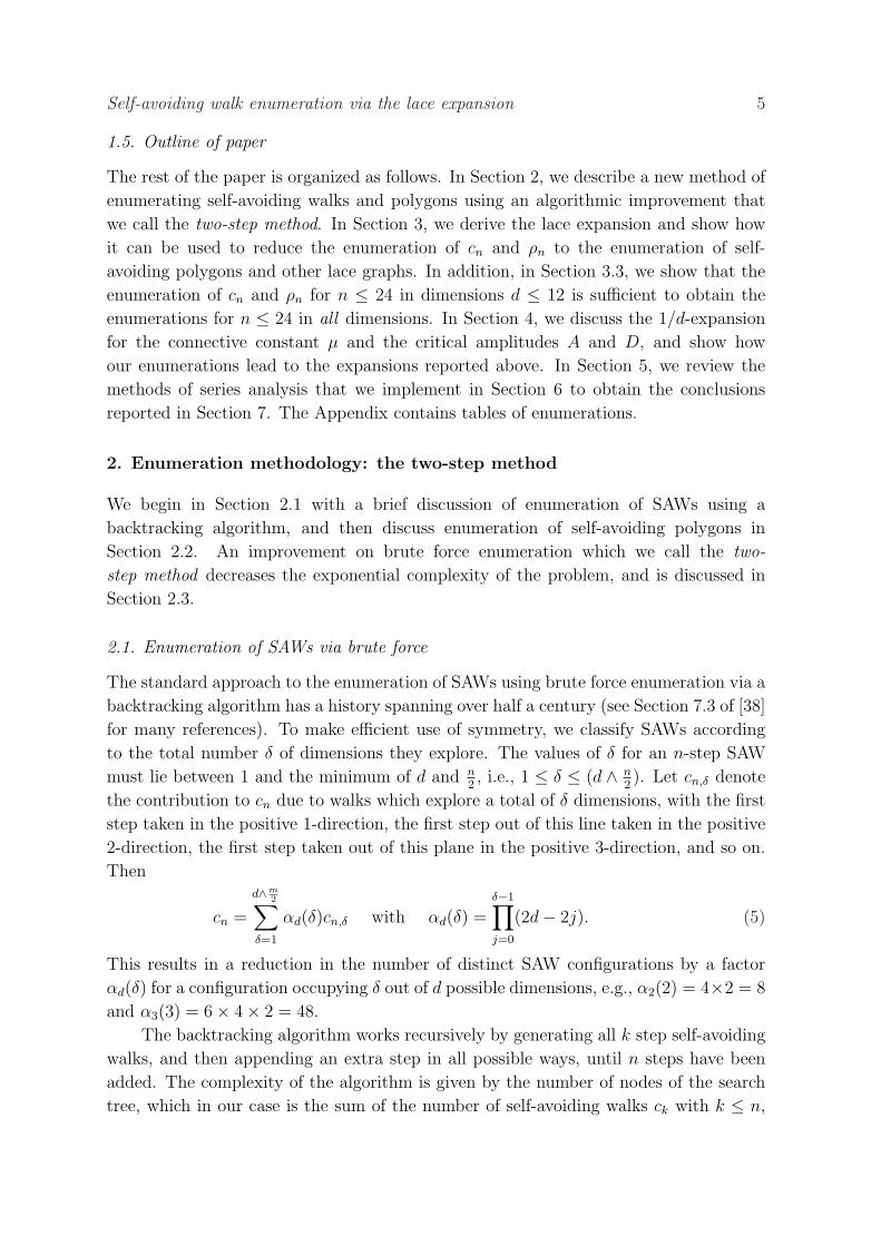
To compute the weight W (Ω) of a 2-step walk, we use the allocation graph
illustrated in Fig. 1 and defined as follows. For a 2-step in which both steps are in
the same direction, we introduce a loop rooted at the midpoint of the 2-step. For a
diagonal 2-step, we introduce an edge which is a perpendicular bisector (in the same
2-dimensional plane as the 2-step itself). The result is the graph GΩ depicted in Fig. 1,
which consists of connected components X (with one loop), Y (with one cycle), and Z
(a tree). We partition the set of connected components of GΩ into the following four
categories:
• TΩ is the set of connected components of GΩ which are trees
• CΩ is the set of connected components of GΩ which contain exactly one cycle but
no loop
• LΩ is the set of connected components of GΩ which contain exactly one loop but
no cycle
• C+Ω is the set of connected components of GΩ in which the number of loops and/or
cycles is at least two.
Let NT denote the number of vertices of a tree T . Finally, we set
IΩ =
1 if C+
Ω = ∅0 otherwise.
(6)
Theorem 2.1. The weight of a 2-step walk Ω is given by
W (Ω) = IΩ2|CΩ|∏
T∈TΩ
NT . (7)
Proof. A SAW consistent with Ω can be regarded as an allocation of a vertex in GΩ to
each 2-step in Ω, subject to the restriction that each 2-step is allocated a distinct vertex
which is a possible intermediate step for that 2-step. We represent this allocation by
an arrow on each edge in GΩ pointing to the chosen vertex, i.e., by an orientation
of the allocation graph. An admissible orientation is one with at most one arrow
pointing towards each vertex, i.e., with in-degree at most 1 at each vertex of the
oriented allocation graph. The weight W (Ω) is thus equal to the number of admissible
Self-avoiding walk enumeration via the lace expansion 8
X
Z
Y
Figure 1. The allocation graph (solid lines) of a 2-step walk (broken lines), withconnected components X, Y , and Z.
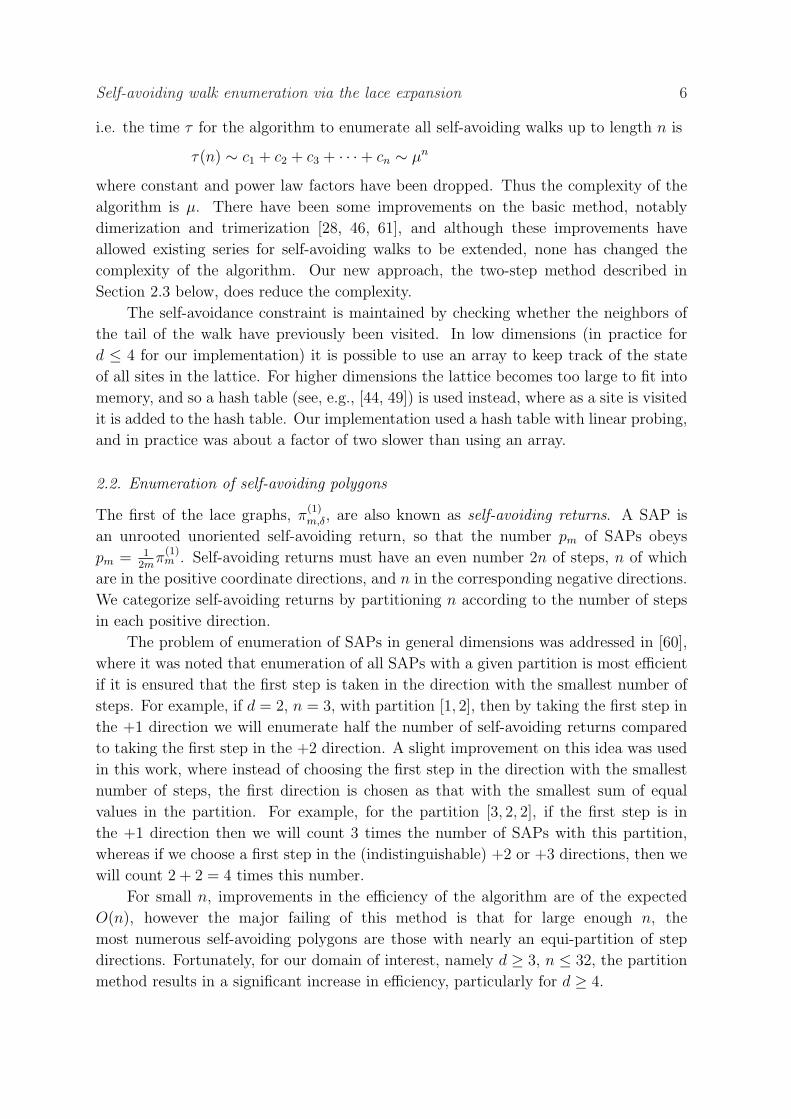
orientations of the allocation graph GΩ. We show the admissible orientations of the
various components of the allocation graph of Fig. 1 in Fig. 2.
It is plain that the number of admissible orientations of GΩ is equal to the product
of the number of admissible orientations of each connected component. For each type
of component, this number is as follows:
• For a tree T ∈ TΩ, an admissible orientation is characterized by a choice of one
vertex to serve as a source, from which all arrows point away. Thus there are NT
admissible orientations.
• For a component in LΩ, removal of the single loop results in a tree, and the arrow
on the loop forces the vertex on the loop to be the source for the tree. Thus there
is exactly one admissible orientation.
• For a component in CΩ, there are two ways to orient the cycle, and each choice
allocates sources for any branches off the cycle. Thus there are exactly two
admissible orientations.
• There are no admissible allocations for a component in C+Ω . This is easily verified
for cycles which overlap in the form of a Θ and also for dumbbell graphs, and the
general case is similar.
Together, these observations complete the proof.
The data structure that we implement to represent an allocation graph must be
able to perform several operations quickly for dynamical backtracking, such as pruning
a tree, concatenation of components, identifying the size of a tree, and so on. It is
straightforward to construct a data structure which allows these operations, so we do
not give the details of our choice here. In our implementation, it takes O(log n) time,
for a tree of n vertices, to perform the query operations, and O(1) time to perform the
other operations.
The extension of the two-step method to the enumeration of self-avoiding polygons
is straightforward, even when combined with the partitioning of step directions as
described in Section 2.2.
Self-avoiding walk enumeration via the lace expansion 9
Figure 2. Admissible orientations of the connected components of the allocationgraph of Fig. 1.
Complexity of the two-step and k-step methods
It is natural to ask why we are only using the two-step method, rather than the three-
step, four-step, or k-step methods. Our partial answer to this question has to do with the
computational complexity of the k-step methods. Suppose that we wish to enumerate
all SAWs of length n = kl. There are two aspects to the computational complexity:
the time required to enumerate all k-step walks of length l, and the time required to
compute the weight of each of these k-step walks. Let us begin with the first of these
issues.
The usual subadditivity argument [29] shows that the number C(k)l of k-step walks
of length l grows exponentially with some growth rate λ = λk. Easy upper and lower
bounds on λ can be calculated in the usual way. For the upper bound, if we only disallow
immediate reversals then we see that if S is the number of sites reachable by a SAW in
k steps, then
C(k)l ≤ S(S − 1)l−1 = S(S − 1)(n−k)/k. (8)
In particular, for k = 2, since S = 8 for the square lattice this gives
λ2 ≤√
7 = 2.645 · · · , (9)
and since S = 18 for the simple cubic lattice, it gives
λ2 ≤√
17 = 4.123 · · · . (10)
A generalization even to three-step would result in a significant improvement in this
upper bound, since for the simple cubic lattice there are S = 44 potential end sites in
three steps, and hence
λ3 ≤ 3√
S − 1 = 3.503 · · · . (11)
Note that exponential lower bounds on C(k)l can also easily be computed. For
example, for k = 2, if we allow 2-steps only in the positive coordinate directions on the
d-dimensional cubic lattice then we see that
C(2)l ≥ (
d +(
d2
))l=
(d +
(d2
))n/2, (12)
Self-avoiding walk enumeration via the lace expansion 10
and hence
λ2 ≥√
d +(
d2
). (13)
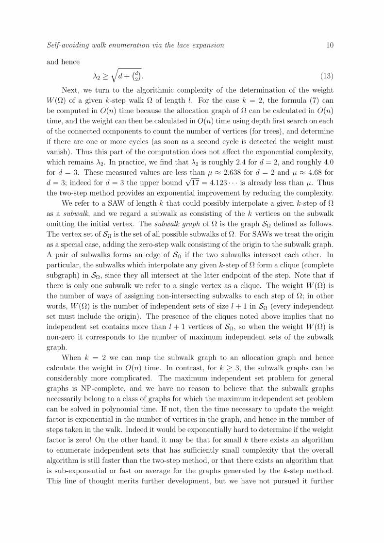
Next, we turn to the algorithmic complexity of the determination of the weight
W (Ω) of a given k-step walk Ω of length l. For the case k = 2, the formula (7) can
be computed in O(n) time because the allocation graph of Ω can be calculated in O(n)
time, and the weight can then be calculated in O(n) time using depth first search on each
of the connected components to count the number of vertices (for trees), and determine
if there are one or more cycles (as soon as a second cycle is detected the weight must
vanish). Thus this part of the computation does not affect the exponential complexity,
which remains λ2. In practice, we find that λ2 is roughly 2.4 for d = 2, and roughly 4.0
for d = 3. These measured values are less than µ ≈ 2.638 for d = 2 and µ ≈ 4.68 for
d = 3; indeed for d = 3 the upper bound√
17 = 4.123 · · · is already less than µ. Thus
the two-step method provides an exponential improvement by reducing the complexity.
We refer to a SAW of length k that could possibly interpolate a given k-step of Ω
as a subwalk, and we regard a subwalk as consisting of the k vertices on the subwalk
omitting the initial vertex. The subwalk graph of Ω is the graph SΩ defined as follows.
The vertex set of SΩ is the set of all possible subwalks of Ω. For SAWs we treat the origin
as a special case, adding the zero-step walk consisting of the origin to the subwalk graph.
A pair of subwalks forms an edge of SΩ if the two subwalks intersect each other. In
particular, the subwalks which interpolate any given k-step of Ω form a clique (complete
subgraph) in SΩ, since they all intersect at the later endpoint of the step. Note that if
there is only one subwalk we refer to a single vertex as a clique. The weight W (Ω) is
the number of ways of assigning non-intersecting subwalks to each step of Ω; in other
words, W (Ω) is the number of independent sets of size l + 1 in SΩ (every independent
set must include the origin). The presence of the cliques noted above implies that no
independent set contains more than l + 1 vertices of SΩ, so when the weight W (Ω) is
non-zero it corresponds to the number of maximum independent sets of the subwalk
graph.
When k = 2 we can map the subwalk graph to an allocation graph and hence
calculate the weight in O(n) time. In contrast, for k ≥ 3, the subwalk graphs can be
considerably more complicated. The maximum independent set problem for general
graphs is NP-complete, and we have no reason to believe that the subwalk graphs
necessarily belong to a class of graphs for which the maximum independent set problem
can be solved in polynomial time. If not, then the time necessary to update the weight
factor is exponential in the number of vertices in the graph, and hence in the number of
steps taken in the walk. Indeed it would be exponentially hard to determine if the weight
factor is zero! On the other hand, it may be that for small k there exists an algorithm
to enumerate independent sets that has sufficiently small complexity that the overall
algorithm is still faster than the two-step method, or that there exists an algorithm that
is sub-exponential or fast on average for the graphs generated by the k-step method.
This line of thought merits further development, but we have not pursued it further

Self-avoiding walk enumeration via the lace expansion 11
here, and we performed our enumerations using k = 2.
2.4. Parallelization of the algorithm
In order to perform the enumeration of lace graphs and polygons in a reasonable amount
of (calendar) time, it is necessary to divide the workload among many computers. It
is possible to parallelize backtracking algorithms by truncating the backtracking tree
at a fixed level, and dividing the computation beyond that level between different
machines. We did this in the enumeration of polygons and lace graphs (defined in
Section 3), by truncating the backtracking tree at 6 and 8 steps respectively, and
saving the configurations so generated to a file. We then split the file in order to
run the backtracking algorithm with distinct sets of starting configurations on multiple
machines.
3. The lace expansion
In Sections 3.1–3.2, we give a quick sketch of the derivation of the lace expansion, which
is the basis of our method. Further details can be found in the original paper [4], or,
for a more recent account, [59]. In Sections 3.3–3.4, we discuss the enumeration of the
lace graphs.
3.1. The recursion relation
Let c0(x) = δ0,x, and, for n ≥ 1, let cn(x) denote the number of n-step self-avoiding
walks that begin at the origin and end at x ∈ Zd. The lace expansion gives rise to a
function πm(x), defined below, such that for n ≥ 1,
cn(x) =∑
y∈Zd:|y|=1
cn−1(x− y) +n∑
m=2
∑
y∈Zd
πm(y)cn−m(x− y). (14)
Let D(x) = 12d
if |x| = 1 and otherwise D(x) = 0, and let f(k) =∑
x∈Zd f(x)eik·x
(for k = (k1, . . . , kj) ∈ [−π, π]d) denote the Fourier transform of the function f . Then
D(k) = d−1∑d
j=1 cos kj. Fourier transformation of (14) gives
cn(k) = 2dD(k)cn−1(k) +n∑
m=2
πm(k)cn−m(k). (15)
In particular, since cn = cn(0), if we write πm = πm(0) then (15) yields
cn = 2dcn−1 +n∑
m=2
πmcn−m. (16)
Thus knowledge of the coefficients πm for 2 ≤ m ≤ n allows for the recursive
determination of cn.
Self-avoiding walk enumeration via the lace expansion 12
Let ρn =∑
x |x|2cn(x) and rm =∑
x |x|2πm(x). Application of −∑di=1
∂2
∂k2i
∣∣∣k=0
to
(15) leads to the recursion
ρn = 2dcn−1 + 2dρn−1 +n∑
m=2
rmcn−m +n∑
m=2
πmρn−m. (17)
Thus knowledge of the coefficients cm, πm, rm for 2 ≤ m ≤ n allows for the recursive
determination of ρn.
3.2. Definition of πm(x)
In this section, we define πm(x) and sketch the derivation of (14). Let Wm(x) denote
the set of all m-step simple random walk paths (possibly self-intersecting) that start at
the origin and end at x. Given ω ∈ Wm(x), let
Ust(ω) =
−1 if ω(s) = ω(t)
0 if ω(s) 6= ω(t).(18)
Then
cn(x) =∑
ω∈Wn(x)
∏0≤s<t≤n
(1 + Ust(ω)), (19)
since the product is equal to 1 if ω is a self-avoiding walk and is equal to 0 otherwise.
We call any set of pairs st, with s < t chosen from 0, 1, 2, . . . , n, a graph. Let Bn
denote the set of all graphs. Expansion of the product in (19) gives
cn(x) =∑
ω∈Wn(x)
∑Γ∈Bn
∏st∈Γ
Ust(ω). (20)
A graph Γ ∈ Bn is said to be connected‡ if both 0 and n are endpoints of edges in
Γ, and if in addition, for any integer c ∈ (0, n), there are s, t ∈ [0, n] such that s < c < t
and st ∈ Γ. In other words, Γ is connected if, as intervals of real numbers, ∪st∈Γ(s, t)
is equal to the connected interval (0, n). The set of all connected graphs on [0, n] is
denoted Gn. If we partition the sum over connected graphs according to whether: (a) 0
does not occur in an edge in the graph, or (b) 0 does occur in an edge, then we are led
to the identity (14) with
πm(x) =∑
ω∈Wm(x)
∑Γ∈Gm
∏st∈Γ
Ust(ω). (21)
Case (a) gives rise to the first term on the right-hand side of (14), and case (b) gives
rise to the second term, with [0,m] the extent of the connected component containing
0.
An important alternate representation for πm(x) can be obtained in terms of laces.
A lace is a minimally connected graph, i.e., a connected graph for which the removal of
any edge would result in a disconnected graph. The set of laces on [0,m] is denoted by
‡ This is not the standard graph-theory definition of a connected graph.
Self-avoiding walk enumeration via the lace expansion 13
s1 t1 s1 s2 t1 t2
s1 s2 t1 s3 t2 t3 s1 s2 t1 s3 t2 s4 t3 t4
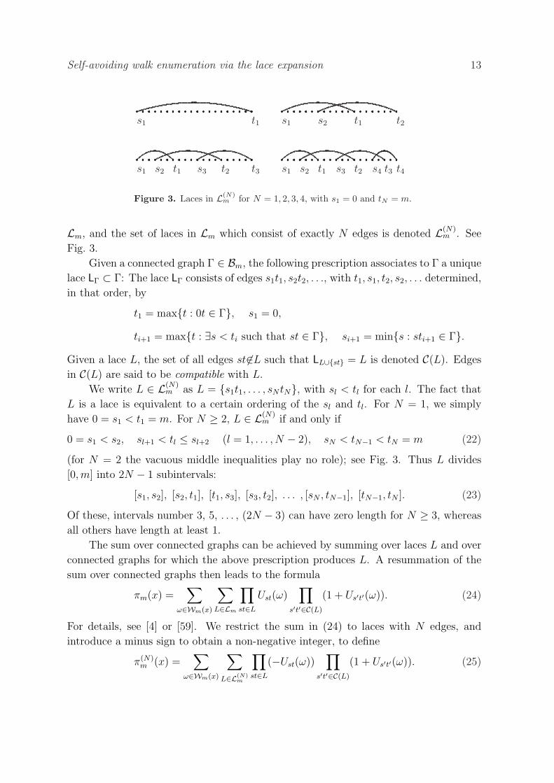
Figure 3. Laces in L(N)m for N = 1, 2, 3, 4, with s1 = 0 and tN = m.
Lm, and the set of laces in Lm which consist of exactly N edges is denoted L(N)m . See
Fig. 3.
Given a connected graph Γ ∈ Bm, the following prescription associates to Γ a unique
lace LΓ ⊂ Γ: The lace LΓ consists of edges s1t1, s2t2, . . ., with t1, s1, t2, s2, . . . determined,
in that order, by
t1 = maxt : 0t ∈ Γ, s1 = 0,
ti+1 = maxt : ∃s < ti such that st ∈ Γ, si+1 = mins : sti+1 ∈ Γ.Given a lace L, the set of all edges st 6∈L such that LL∪st = L is denoted C(L). Edges
in C(L) are said to be compatible with L.
We write L ∈ L(N)m as L = s1t1, . . . , sN tN, with sl < tl for each l. The fact that
L is a lace is equivalent to a certain ordering of the sl and tl. For N = 1, we simply
have 0 = s1 < t1 = m. For N ≥ 2, L ∈ L(N)m if and only if
0 = s1 < s2, sl+1 < tl ≤ sl+2 (l = 1, . . . , N − 2), sN < tN−1 < tN = m (22)
(for N = 2 the vacuous middle inequalities play no role); see Fig. 3. Thus L divides
[0,m] into 2N − 1 subintervals:
[s1, s2], [s2, t1], [t1, s3], [s3, t2], . . . , [sN , tN−1], [tN−1, tN ]. (23)
Of these, intervals number 3, 5, . . . , (2N − 3) can have zero length for N ≥ 3, whereas
all others have length at least 1.
The sum over connected graphs can be achieved by summing over laces L and over
connected graphs for which the above prescription produces L. A resummation of the
sum over connected graphs then leads to the formula
πm(x) =∑
ω∈Wm(x)
∑L∈Lm
∏st∈L
Ust(ω)∏
s′t′∈C(L)
(1 + Us′t′(ω)). (24)
For details, see [4] or [59]. We restrict the sum in (24) to laces with N edges, and
introduce a minus sign to obtain a non-negative integer, to define
π(N)m (x) =
∑
ω∈Wm(x)
∑
L∈L(N)m
∏st∈L
(−Ust(ω))∏
s′t′∈C(L)
(1 + Us′t′(ω)). (25)
Self-avoiding walk enumeration via the lace expansion 14
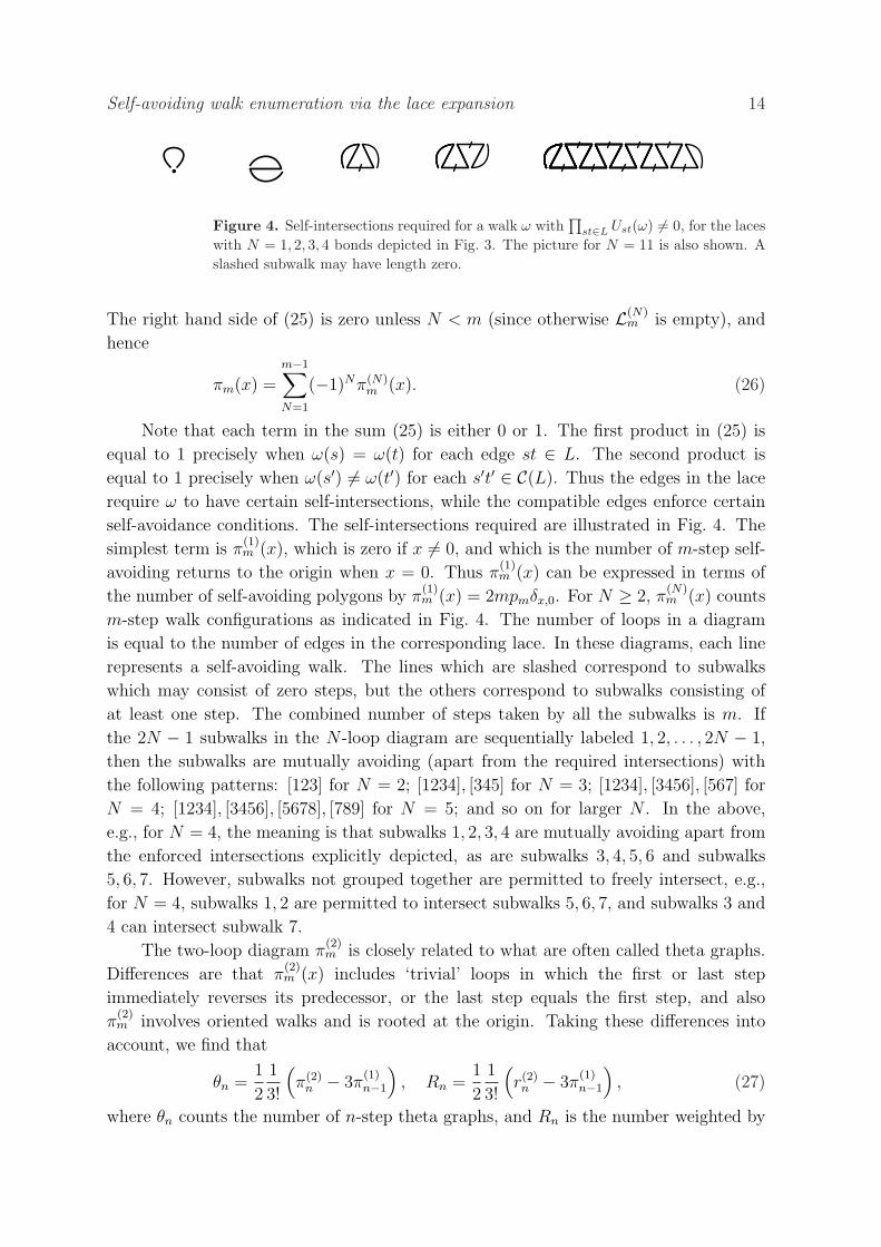
Figure 4. Self-intersections required for a walk ω with∏
st∈L Ust(ω) 6= 0, for the laceswith N = 1, 2, 3, 4 bonds depicted in Fig. 3. The picture for N = 11 is also shown. Aslashed subwalk may have length zero.
The right hand side of (25) is zero unless N < m (since otherwise L(N)m is empty), and
hence
πm(x) =m−1∑N=1
(−1)Nπ(N)m (x). (26)
Note that each term in the sum (25) is either 0 or 1. The first product in (25) is
equal to 1 precisely when ω(s) = ω(t) for each edge st ∈ L. The second product is
equal to 1 precisely when ω(s′) 6= ω(t′) for each s′t′ ∈ C(L). Thus the edges in the lace
require ω to have certain self-intersections, while the compatible edges enforce certain
self-avoidance conditions. The self-intersections required are illustrated in Fig. 4. The
simplest term is π(1)m (x), which is zero if x 6= 0, and which is the number of m-step self-
avoiding returns to the origin when x = 0. Thus π(1)m (x) can be expressed in terms of
the number of self-avoiding polygons by π(1)m (x) = 2mpmδx,0. For N ≥ 2, π
(N)m (x) counts
m-step walk configurations as indicated in Fig. 4. The number of loops in a diagram
is equal to the number of edges in the corresponding lace. In these diagrams, each line
represents a self-avoiding walk. The lines which are slashed correspond to subwalks
which may consist of zero steps, but the others correspond to subwalks consisting of
at least one step. The combined number of steps taken by all the subwalks is m. If
the 2N − 1 subwalks in the N -loop diagram are sequentially labeled 1, 2, . . . , 2N − 1,
then the subwalks are mutually avoiding (apart from the required intersections) with
the following patterns: [123] for N = 2; [1234], [345] for N = 3; [1234], [3456], [567] for
N = 4; [1234], [3456], [5678], [789] for N = 5; and so on for larger N . In the above,
e.g., for N = 4, the meaning is that subwalks 1, 2, 3, 4 are mutually avoiding apart from
the enforced intersections explicitly depicted, as are subwalks 3, 4, 5, 6 and subwalks
5, 6, 7. However, subwalks not grouped together are permitted to freely intersect, e.g.,
for N = 4, subwalks 1, 2 are permitted to intersect subwalks 5, 6, 7, and subwalks 3 and
4 can intersect subwalk 7.
The two-loop diagram π(2)m is closely related to what are often called theta graphs.
Differences are that π(2)m (x) includes ‘trivial’ loops in which the first or last step
immediately reverses its predecessor, or the last step equals the first step, and also
π(2)m involves oriented walks and is rooted at the origin. Taking these differences into
account, we find that
θn =1
2
1
3!
(π(2)
n − 3π(1)n−1
), Rn =
1
2
1
3!
(r(2)n − 3π
(1)n−1
), (27)
where θn counts the number of n-step theta graphs, and Rn is the number weighted by
Self-avoiding walk enumeration via the lace expansion 15
the square of the distance between the two vertices of degree 3.
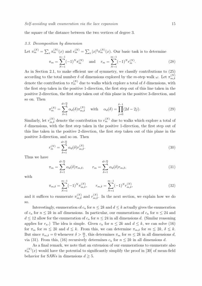
3.3. Decomposition by dimension
Let π(N)m =
∑x π
(N)m (x) and r
(N)m =
∑x |x|2π(N)
m (x). Our basic task is to determine
πm =m−1∑N=1
(−1)Nπ(N)m and rm =
m−1∑N=1
(−1)Nr(N)m . (28)
As in Section 2.1, to make efficient use of symmetry, we classify contributions to (25)
according to the total number δ of dimensions explored by the m-step walk ω. Let π(N)m,δ
denote the contribution to π(N)m due to walks which explore a total of δ dimensions, with
the first step taken in the positive 1-direction, the first step out of this line taken in the
positive 2-direction, the first step taken out of this plane in the positive 3-direction, and
so on. Then
π(N)m =
d∧m2∑
δ=1
αd(δ)π(N)m,δ with αd(δ) =
δ−1∏j=0
(2d− 2j). (29)
Similarly, let r(N)m,δ denote the contribution to r
(N)m due to walks which explore a total of
δ dimensions, with the first step taken in the positive 1-direction, the first step out of
this line taken in the positive 2-direction, the first step taken out of this plane in the
positive 3-direction, and so on. Then
r(N)m =
d∧m2∑
δ=1
αd(δ)r(N)m,δ . (30)
Thus we have
πm =
d∧m2∑
δ=1
αd(δ)πm,δ, rm =
d∧m2∑
δ=1
αd(δ)rm,δ, (31)
with
πm,δ =m−1∑N=1
(−1)Nπ(N)m,δ , rm,δ =
m−1∑N=1
(−1)Nr(N)m,δ , (32)
and it suffices to enumerate π(N)m,δ and r
(N)m,δ . In the next section, we explain how we do
so.
Interestingly, enumeration of cn for n ≤ 2k and d ≤ k actually gives the enumeration
of cn for n ≤ 2k in all dimensions. In particular, our enumerations of cn for n ≤ 24 and
d ≤ 12 allow for the enumeration of cn for n ≤ 24 in all dimensions d. (Similar reasoning
applies for rn.) The idea is simple. Given cn for n ≤ 2k and d ≤ k, we can solve (16)
for πm for m ≤ 2k and d ≤ k. From this, we can determine πm,δ for m ≤ 2k, δ ≤ k.
But since πm,δ = 0 whenever δ > m2, this determines πm for m ≤ 2k in all dimensions d,
via (31). From this, (16) recursively determines cn for n ≤ 2k in all dimensions d.
As a final remark, we note that an extension of our enumerations to enumerate also
π(N)m (x) would have the potential to significantly simplify the proof in [30] of mean-field
behavior for SAWs in dimensions d ≥ 5.
Self-avoiding walk enumeration via the lace expansion 16
ω1 2ω
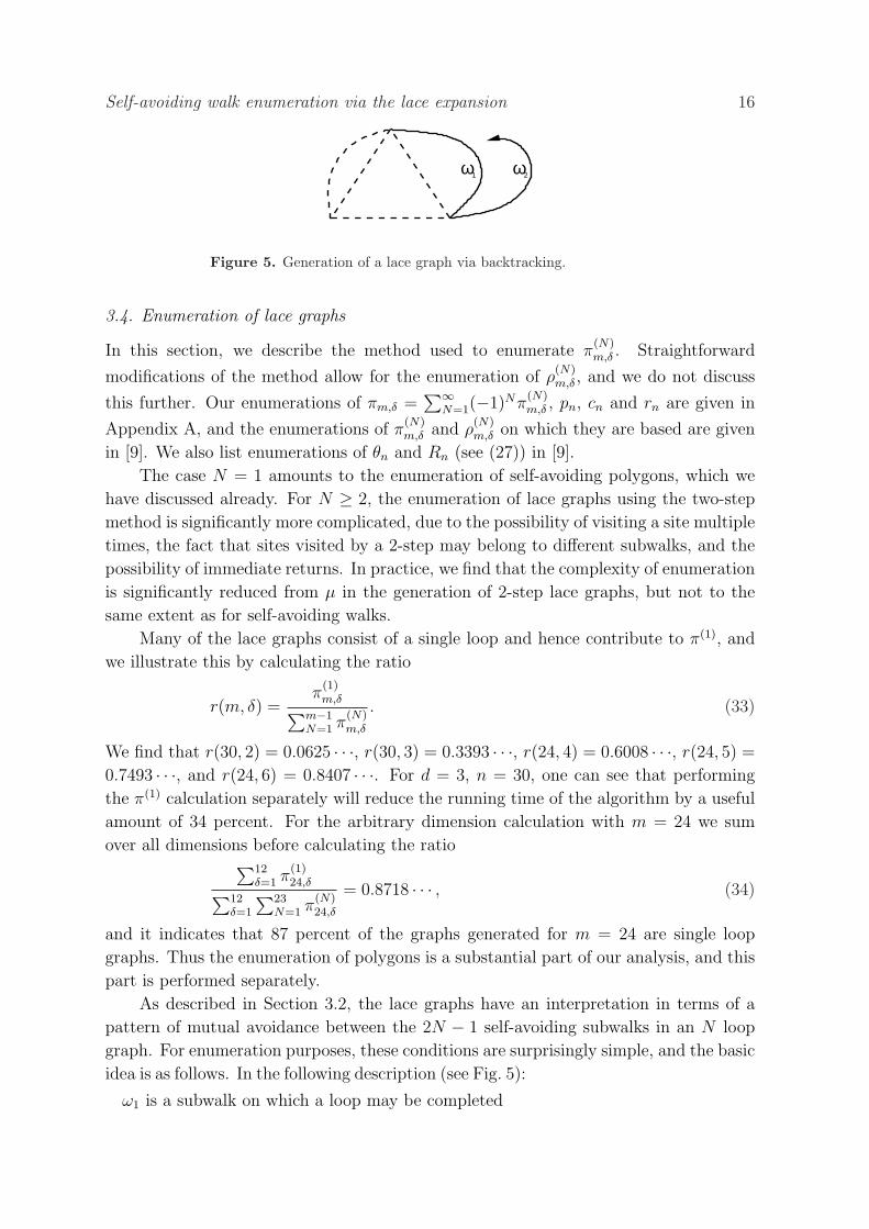
Figure 5. Generation of a lace graph via backtracking.
3.4. Enumeration of lace graphs
In this section, we describe the method used to enumerate π(N)m,δ . Straightforward
modifications of the method allow for the enumeration of ρ(N)m,δ , and we do not discuss
this further. Our enumerations of πm,δ =∑∞
N=1(−1)Nπ(N)m,δ , pn, cn and rn are given in
Appendix A, and the enumerations of π(N)m,δ and ρ
(N)m,δ on which they are based are given
in [9]. We also list enumerations of θn and Rn (see (27)) in [9].
The case N = 1 amounts to the enumeration of self-avoiding polygons, which we
have discussed already. For N ≥ 2, the enumeration of lace graphs using the two-step
method is significantly more complicated, due to the possibility of visiting a site multiple
times, the fact that sites visited by a 2-step may belong to different subwalks, and the
possibility of immediate returns. In practice, we find that the complexity of enumeration
is significantly reduced from µ in the generation of 2-step lace graphs, but not to the
same extent as for self-avoiding walks.
Many of the lace graphs consist of a single loop and hence contribute to π(1), and
we illustrate this by calculating the ratio
r(m, δ) =π
(1)m,δ∑m−1
N=1 π(N)m,δ
. (33)
We find that r(30, 2) = 0.0625 · · ·, r(30, 3) = 0.3393 · · ·, r(24, 4) = 0.6008 · · ·, r(24, 5) =
0.7493 · · ·, and r(24, 6) = 0.8407 · · ·. For d = 3, n = 30, one can see that performing
the π(1) calculation separately will reduce the running time of the algorithm by a useful
amount of 34 percent. For the arbitrary dimension calculation with m = 24 we sum
over all dimensions before calculating the ratio∑12
δ=1 π(1)24,δ∑12
δ=1
∑23N=1 π
(N)24,δ
= 0.8718 · · · , (34)
and it indicates that 87 percent of the graphs generated for m = 24 are single loop
graphs. Thus the enumeration of polygons is a substantial part of our analysis, and this
part is performed separately.
As described in Section 3.2, the lace graphs have an interpretation in terms of a
pattern of mutual avoidance between the 2N − 1 self-avoiding subwalks in an N loop
graph. For enumeration purposes, these conditions are surprisingly simple, and the basic
idea is as follows. In the following description (see Fig. 5):
ω1 is a subwalk on which a loop may be completed
Self-avoiding walk enumeration via the lace expansion 17
ω2 is the current subwalk, which must be avoided, and
the tail of the walk is the last visited site.
First a self-avoiding return is formed, and the count for π(1) is incremented. Then ω1
is set as the loop, and ω2 is set as the origin. Steps are added to the graph, namely to
subwalk ω2, such that ω2 remains self-avoiding. When contact is made with ω1 a loop
is formed and hence this configuration contributes to π(2), and then the current ω1 is
erased, and ω1 is set to the old ω2, while ω2 is just set as the tail of the walk. This
procedure is then repeated, as shown schematically in Fig. 5, where the part of the walk
with a dashed line has been erased. Steps are added in a self-avoiding way to ω2 until
the tail reaches a site on ω1, at which point the count for π(N) is updated, ω1 is erased
and the process starts again.
We initialize the system as follows:
N ⇐ 0 N is the number of loopsm ⇐ 0 m is the lengthδ ⇐ 0
All π(N)m,δ set to 0
Set walk ω1 to be the origin
Set walk ω2 to be empty
Set the origin to be occupied
tail ⇐ origin
The procedure is described more precisely by the following pseudocode:
Recursive procedure, Enumerate lace:
for all s ∈ neighborhood(tail) do
m ⇐ m + 1
if step explores a new dimension then
δ ⇐ δ + 1
end if
if s is empty then
ω2 ⇐ ω2 : s append s to ω2Set s to be occupied
tail ⇐ s
Call Enumerate lace
else if s ∈ ω1 then
N ⇐ N + 1 a loop has been completedπ
(N)m,δ ⇐ π
(N)m,δ + 1 increment count
ω1 ⇐ ω2
ω2 ⇐ s
tail ⇐ s
Call Enumerate lace
else if s ∈ ω2 then
Do nothing reject this step

Self-avoiding walk enumeration via the lace expansion 18
end if
Restore configuration
end for
Return
The exponential complexity of the algorithm will not change depending on the
implementation, but it is possible to make gains in the power of n which is a factor,
so we make efforts to obtain an efficient implementation. Some general considerations
given on backtracking algorithms in the context of search and existence algorithms in [50]
apply also for enumeration applications. For algorithms with exponential complexity,
the operations which dominate the running time of the algorithm are near the leaves
of the tree. This observation leads to two main conclusions regarding the design of
backtracking algorithms: (a) If an expensive operation near the root of the tree can
limit the number of leaves of the tree, then it will reduce the run time of the algorithm
(i.e., prune near the root), and (b) Near the leaves of the tree it is important to have
the basic operations run as rapidly as possible.
Our implementation used doubly linked lists for the subwalks ω1 and ω2, and
satisfied (a) by terminating the backtracking tree whenever it could be determined
that it is impossible due to geometric constraints to generate a valid lace graph from
the current configuration. We implemented a fast heuristic operation to do this which
takes time that is linear in the number of sites that are potential endpoints of a lace
graph generated from the current configuration. In order to satisfy (b) we optimized
the treatment of the final four steps by writing separate code which eliminated any
expensive operations on the linked list structures.
One further technical point is that there is a bijection between lace graphs of m+1
steps which return immediately to the origin with their second step, and lace graphs of
m steps. In our implementation, we forbade this initial immediate return, and it was a
simple process to extract the correct π(N)m,δ from the resulting enumerations.
4. Expansions in powers of 1/d
In this section, we explain how to combine our enumerations with estimates on the lace
expansion to derive the 1/d expansions (1), (3) and (4) for the connective constant µ
and for the amplitudes A and D. Let zc = 1/µ denote the radius of convergence of the
susceptibility χ(z) =∑∞
n=0 cnzn. We will rely on the standard lace expansion estimate
that for each N ≥ 1 there is a constant CN , independent of sufficiently large d, such
that∞∑
m=2
∞∑M=N
mπ(M)m zm
c ≤ CNd−N ,
∞∑m=2
∞∑M=N
r(M)m zm
c ≤ CNd−N . (35)
The bounds (35) can be gleaned, e.g., from Section 5.4 and the solution to Exercise 5.17
of [59] ([30] has related bounds valid for all d ≥ 5). We will supplement (35) by proving
Self-avoiding walk enumeration via the lace expansion 19
that for each j ≥ 2, N ≥ 1, there is a constant CN,j, independent of large d, such that∞∑
m=j
mπ(N)m zm
c ≤ CN,jd−j/2,
∞∑m=j
r(N)m zm
c ≤ CN,jd−j/2. (36)
4.1. 1/d expansion for the connective constant
It is proved in [31] that, for d ≥ 5, zc obeys the equation
zc =1
2d
[1−
∞∑m=2
πmzmc
]. (37)
It then follows from the first estimates of (35) and (36) that
zc =1
2d
[1−
2N∑m=2
N∑M=1
(−1)Mπ(M)m zm
c
]+ O(d−N−2), (38)
where we have used the fact proved in [32] that zc has an asymptotic expansion in powers
of d−1, to replace an error term of order d−N−3/2 by one of order d−N−2. Knowledge of
the coefficients π(M)m for m ≤ 2N and M ≤ N permits the recursive calculation of the
terms in the 1/d expansion for zc up to and including order d−N−1. Our enumerations
with m ≤ 24, M ≤ 12 give
zc =1
2d+
1
(2d)2+
2
(2d)3+
6
(2d)4+
27
(2d)5+
157
(2d)6+
1065
(2d)7+
7865
(2d)8+
59665
(2d)9
+422421
(2d)10+
1991163
(2d)11− 16122550
(2d)12− 805887918
(2d)13+ O
(1
(2d)14
). (39)
Taking the reciprocal gives the 1/d expansion for µ stated in (1).
4.2. 1/d expansion for the amplitudes A and D
It is proved in [31] that for d ≥ 5 the amplitudes A and D of (2) are given by the
formulas
1
A= 2dzc +
∞∑m=2
mπmzmc , D = A
[2dzc +
∞∑m=2
rmzmc
]. (40)
It then follows from (35) and (36) that
1
A= 2dzc +
2N∑m=2
N∑M=1
(−1)Mmπ(M)m zm
c + O(d−N−1) (41)
and
D = A
[2dzc +
2N∑m=2
N∑M=1
(−1)Mr(M)m zm
c
]+ O(d−N−1). (42)
Note that there can again be no fractional powers in the error estimates — it can be
argued from the fact that zc has an asymptotic expansion to all orders in powers of d−1,
together with the representations of π(M)m and r
(M)n as polynomials in d in (31), that A

Self-avoiding walk enumeration via the lace expansion 20
and D also have asymptotic expansions to all orders in powers of d−1. Insertion of (39)
and our enumerations for m ≤ 24, M ≤ 12 into (41) and (42) gives the series (3) and
(4).
4.3. Proof of the error estimates (36)
It remains to prove (36). We do so in the rest of this section, by making use of notation
and results from Chapters 4 and 5 of [59], and of Chapter 6 of [48] (see [35] for related
ideas applied to percolation). We assume throughout this section that d is large, and
we write c for a constant, possibly depending on N and j but independent of d, whose
value is unimportant and may change from line to line.
Preliminaries
We will need the norms ‖f‖∞ = supx∈Zd |f(x)| and ‖f‖2 = [∑
x∈Zd |f(x)|2]1/2 for
functions f : Zd → R, and also the norms ‖f‖p = [(2π)−d∫[−π,π]d
|f(k)|pdk]1/p for
the Fourier transform f(k) =∑
x∈Zd f(x)eik·x. The inverse Fourier transform is given
by f(x) = (2π)−d∫[−π,π]d
f(k)e−ik·xdk, from which we conclude that ‖f‖∞ ≤ ‖f‖1. The
Parseval relation asserts that ‖f‖2 = ‖f‖2. The convolution (f∗g)(x) =∑
y f(y−x)g(y)
obeys ‖f ∗ g‖∞ ≤ ‖f‖2‖g‖2, by the Cauchy–Schwarz inequality, and f ∗ g = f g.
Let D : Zd → R be the one-step transition probability for simple random walk,
i.e., D(x) = 12d
if |x| = 1 and otherwise D(x) = 0. Let D∗l denote the convolution of l
factors of D, so that D∗l(x) is the probability that simple random walk goes from 0 to
x in l steps. It is an elementary fact that the probability that a simple random walk on
Zd returns to its starting point after 2i steps obeys
D∗(2i)(0) =
∫
[−π,π]dD(k)2i dk
(2π)d= ‖Di‖2
2 ≤ cid−i (43)
with ci independent of the dimension d (see (3.12) of [35] for a simple proof). By the
Cauchy–Schwarz inequality and the Parseval relation, it follows that
‖D∗j‖∞ ≤ ‖D∗(j−1)‖2‖D‖2 = ‖Dj−1‖2‖D‖2 ≤ cd−j/2, (44)
and it is this inequality that will give us the desired factor d−j/2 in (36). Direct
calculation gives D(k) = 1d
∑dj=1 cos kj for k = (k1, . . . , kd), and hence
∂jD(k) = −1
dsin kj, ∂2
j D(k) = −1
dcos kj, (45)
where ∂j denotes differentiation with respect to kj.
Let Gzc(x) =∑∞
m=0 cm(x)zmc . It is shown in Corollary 6.2.6 of [48] that ‖Gzc‖2 is
bounded by a d-independent constant. In addition, ‖Gzc ∗Gzc‖2 = ‖Gzc‖24, and ‖Gzc‖p is
bounded by a d-independent constant, for any fixed p, if d is sufficiently large (depending
on p). This can be shown using the infrared bound Gzc(k) ≤ [1−D(k)]−1 given in (6.2.19)
of [48] or (5.36) of [59] (see Exercise 5.18(a) of [59] for the d-independence of the upper
bound).
Self-avoiding walk enumeration via the lace expansion 21
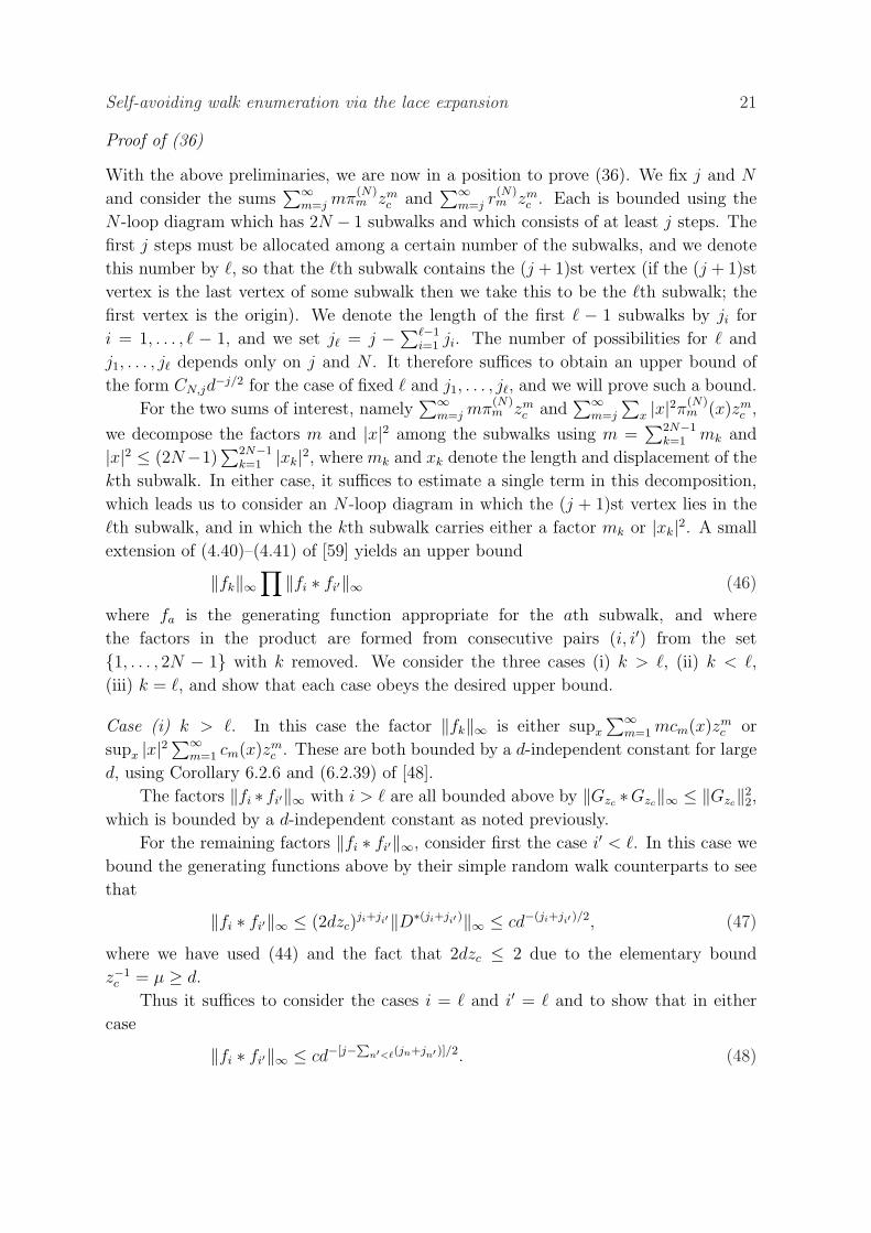
Proof of (36)
With the above preliminaries, we are now in a position to prove (36). We fix j and N
and consider the sums∑∞
m=j mπ(N)m zm
c and∑∞
m=j r(N)m zm
c . Each is bounded using the
N -loop diagram which has 2N − 1 subwalks and which consists of at least j steps. The
first j steps must be allocated among a certain number of the subwalks, and we denote
this number by `, so that the `th subwalk contains the (j + 1)st vertex (if the (j + 1)st
vertex is the last vertex of some subwalk then we take this to be the `th subwalk; the
first vertex is the origin). We denote the length of the first ` − 1 subwalks by ji for
i = 1, . . . , ` − 1, and we set j` = j − ∑`−1i=1 ji. The number of possibilities for ` and
j1, . . . , j` depends only on j and N . It therefore suffices to obtain an upper bound of
the form CN,jd−j/2 for the case of fixed ` and j1, . . . , j`, and we will prove such a bound.
For the two sums of interest, namely∑∞
m=j mπ(N)m zm
c and∑∞
m=j
∑x |x|2π(N)
m (x)zmc ,
we decompose the factors m and |x|2 among the subwalks using m =∑2N−1
k=1 mk and
|x|2 ≤ (2N−1)∑2N−1
k=1 |xk|2, where mk and xk denote the length and displacement of the
kth subwalk. In either case, it suffices to estimate a single term in this decomposition,
which leads us to consider an N -loop diagram in which the (j + 1)st vertex lies in the
`th subwalk, and in which the kth subwalk carries either a factor mk or |xk|2. A small
extension of (4.40)–(4.41) of [59] yields an upper bound
‖fk‖∞∏
‖fi ∗ fi′‖∞ (46)
where fa is the generating function appropriate for the ath subwalk, and where
the factors in the product are formed from consecutive pairs (i, i′) from the set
1, . . . , 2N − 1 with k removed. We consider the three cases (i) k > `, (ii) k < `,
(iii) k = `, and show that each case obeys the desired upper bound.
Case (i) k > `. In this case the factor ‖fk‖∞ is either supx
∑∞m=1 mcm(x)zm
c or
supx |x|2∑∞
m=1 cm(x)zmc . These are both bounded by a d-independent constant for large
d, using Corollary 6.2.6 and (6.2.39) of [48].
The factors ‖fi ∗ fi′‖∞ with i > ` are all bounded above by ‖Gzc ∗Gzc‖∞ ≤ ‖Gzc‖22,
which is bounded by a d-independent constant as noted previously.
For the remaining factors ‖fi ∗ fi′‖∞, consider first the case i′ < `. In this case we
bound the generating functions above by their simple random walk counterparts to see
that
‖fi ∗ fi′‖∞ ≤ (2dzc)ji+ji′‖D∗(ji+ji′ )‖∞ ≤ cd−(ji+ji′ )/2, (47)
where we have used (44) and the fact that 2dzc ≤ 2 due to the elementary bound
z−1c = µ ≥ d.
Thus it suffices to consider the cases i = ` and i′ = ` and to show that in either
case
‖fi ∗ fi′‖∞ ≤ cd−[j−Pn′<`(jn+jn′ )]/2. (48)
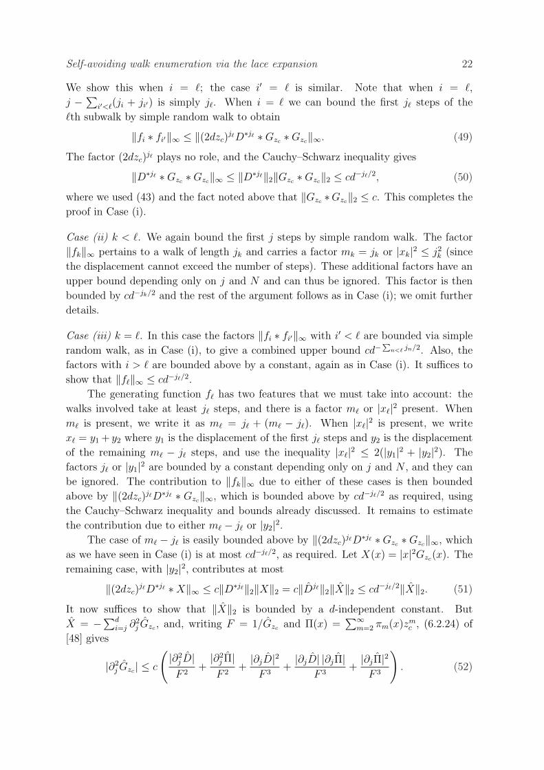
Self-avoiding walk enumeration via the lace expansion 22
We show this when i = `; the case i′ = ` is similar. Note that when i = `,
j − ∑i′<`(ji + ji′) is simply j`. When i = ` we can bound the first j` steps of the
`th subwalk by simple random walk to obtain
‖fi ∗ fi′‖∞ ≤ ‖(2dzc)j`D∗j` ∗Gzc ∗Gzc‖∞. (49)
The factor (2dzc)j` plays no role, and the Cauchy–Schwarz inequality gives
‖D∗j` ∗Gzc ∗Gzc‖∞ ≤ ‖D∗j`‖2‖Gzc ∗Gzc‖2 ≤ cd−j`/2, (50)
where we used (43) and the fact noted above that ‖Gzc ∗Gzc‖2 ≤ c. This completes the
proof in Case (i).
Case (ii) k < `. We again bound the first j steps by simple random walk. The factor
‖fk‖∞ pertains to a walk of length jk and carries a factor mk = jk or |xk|2 ≤ j2k (since
the displacement cannot exceed the number of steps). These additional factors have an
upper bound depending only on j and N and can thus be ignored. This factor is then
bounded by cd−jk/2 and the rest of the argument follows as in Case (i); we omit further
details.
Case (iii) k = `. In this case the factors ‖fi ∗ fi′‖∞ with i′ < ` are bounded via simple
random walk, as in Case (i), to give a combined upper bound cd−P
n<` jn/2. Also, the
factors with i > ` are bounded above by a constant, again as in Case (i). It suffices to
show that ‖f`‖∞ ≤ cd−j`/2.
The generating function f` has two features that we must take into account: the
walks involved take at least j` steps, and there is a factor m` or |x`|2 present. When
m` is present, we write it as m` = j` + (m` − j`). When |x`|2 is present, we write
x` = y1 + y2 where y1 is the displacement of the first j` steps and y2 is the displacement
of the remaining m` − j` steps, and use the inequality |x`|2 ≤ 2(|y1|2 + |y2|2). The
factors j` or |y1|2 are bounded by a constant depending only on j and N , and they can
be ignored. The contribution to ‖fk‖∞ due to either of these cases is then bounded
above by ‖(2dzc)j`D∗j` ∗ Gzc‖∞, which is bounded above by cd−j`/2 as required, using
the Cauchy–Schwarz inequality and bounds already discussed. It remains to estimate
the contribution due to either m` − j` or |y2|2.The case of m` − j` is easily bounded above by ‖(2dzc)
j`D∗j` ∗Gzc ∗Gzc‖∞, which
as we have seen in Case (i) is at most cd−j`/2, as required. Let X(x) = |x|2Gzc(x). The
remaining case, with |y2|2, contributes at most
‖(2dzc)j`D∗j` ∗X‖∞ ≤ c‖D∗j`‖2‖X‖2 = c‖Dj`‖2‖X‖2 ≤ cd−j`/2‖X‖2. (51)
It now suffices to show that ‖X‖2 is bounded by a d-independent constant. But
X = −∑di=j ∂2
j Gzc , and, writing F = 1/Gzc and Π(x) =∑∞
m=2 πm(x)zmc , (6.2.24) of
[48] gives
|∂2j Gzc | ≤ c
(|∂2
j D|F 2
+|∂2
j Π|F 2
+|∂jD|2
F 3+|∂jD| |∂jΠ|
F 3+|∂jΠ|2
F 3
). (52)

Self-avoiding walk enumeration via the lace expansion 23
It suffices to obtain an O(d−1) upper bound on the L2 norm of each term on the right-
hand side.
By (45), the L2 norm of the first term on the right-hand side of (52) is at most
cd−1‖G2zc‖2, which we have seen is O(d−1). It is shown in Corollary 6.2.7 of [48] that
∂aj Π = O(d−2) for a = 1, 2. Together with our previous observation that ‖Gzc‖6 ≤ c,
this is sufficient for our needs and completes the proof of the error estimates (36).
5. Analysis of series: methodology
The presumed asymptotic forms for cn, ρn and pn for d = 3 are given by
cn ∼ µnnγ−1(A +
a1
nθ+
a2
n+
a3
n1+θ+
a4
n2+ · · ·
)
+ µn(−1)nnα−2
(b0 +
b1
nθ+
b2
n+
b3
n1+θ+
b4
n2+ · · ·
), (53)
ρn ∼ µnnγ+2ν−1
(AD +
d1
nθ+
d2
n+
d3
n1+θ+
d4
n2+ · · ·
)
+ µn(−1)nnα−2(e0 +
e1
nθ+
e2
n+
e3
n1+θ+
e4
n2+ · · ·
), (54)
pn ∼ µnnα−3
(B +
f1
nθ+
f2
n+
f3
n1+θ+
f4
n2+ · · ·
)(n even). (55)
The alternating terms in the formulae for cn and ρn are manifestations of a
generating function singularity at −zc = −1/µ. This singularity, widely believed but
not rigorously proved to exist, is known as the anti-ferromagnetic singularity due to
its similarity to a corresponding singularity in the Ising model. Anti-ferromagnetic
singularities are generally expected to occur on loose-packed (certain bipartite) lattices
such as Zd. The fact that the polygon exponent α governs the effect of this singularity
on the series has very strong numerical evidence for d = 2 [7, 41], and was suggested
as early as [22]. As we will argue in [10], the alternating signs in the values of πm
provide direct evidence both for the existence of the anti-ferromagnetic singularity and
the role of α in its behavior (see Tables 16–17 — we believe but have not proved that
the alternation in sign persists for all m).
We find that the conventional assumption (see, e.g., [7, 47]) that the leading
confluent correction θ is the same for cn and ρn is well supported by our results. The
series we have for pn are too short to say anything definitive in this respect. There is
an implicit assumption in the formulae above that θ is close to 0.5 and therefore integer
multiples of the form 2kθ are indistinguishable from integer terms, while (2k+1)θ ≈ k+θ.
If θ is not exactly 0.5 then this assumption must eventually break down for high-order
terms in the asymptotic form.
Series analysis is a collection of methods for estimating the values of µ, γ, ν, α,
etc., given the values of cn, ρn, pn for n ≤ N . For an extensive overview of methods
of series analysis, see [26]. We apply the methods of differential approximants [26] (a
Self-avoiding walk enumeration via the lace expansion 24
generalization of Pade approximants, also called integral approximants [39]), the version
of the ratio method due to Zinn-Justin [62, 63, 26, 5], and direct fitting of the presumed
asymptotic form. In this section, we discuss each of the methods in some detail. (We
have also applied Neville-Aitken extrapolation and the Brezinski θ algorithm [26], but
neither of these methods produced improved results.)
5.1. The method of differential approximants
In the method of differential approximants, the unknown generating function is
represented by the solution to an ordinary differential equation of the form:
K∑i=0
Qi(z)dif
dzi= P (z). (56)
The functions P and Qi are polynomials, of degrees L and Ni. We choose L ≤ 5,
K = 1, 2, 3, NK ≥ 3 (which guarantees at least three regular singularities), and take
QK to have highest-order coefficient equal to 1. The order of the polynomials was
chosen so that |Ni − Nj| ≤ 2. Given coefficients a0, . . . , aN , the polynomials P,Qi are
chosen so that the polynomial∑N
n=0 anzn solves the differential equation to within an
error of order zN+1. This choice is made by solving a system of linear equations in
L + K + 1 +∑K
i=0 Ni unknowns, determined from N + 1 known coefficients.
The series we analyze for d = 3, in particular, produce many defective approximants
which have singularities near the physical singularity, or clearly incorrect singularities
on or near the positive real axis, which may distort estimates of the critical point
and critical exponents. We attribute this, in part, to the existence of strong confluent
corrections. In practice, eliminating defective approximants does not change central
estimates in the series we analyzed significantly, but does slightly reduce the spread of
estimates, and especially for K = 1, 2 and large N , eliminates most of the approximants.
This introduces a systematic bias, and it is primarily for this reason that we chose not
to eliminate defective approximants. Instead we iteratively eliminated outliers in our
analysis, for which the critical point and critical exponents differ from the mean by more
than r times the standard deviation, with the subjective choice r = 3. We report the
standard deviation of the estimates of the remaining approximants, as an indication of
their spread.
It is straightforward to ensure that there is a singularity at a biased value of zc by
introducing an additional linear equation:
QK(zc) = 0. (57)
It is less straightforward to bias the exponent without simultaneously fixing the critical
point, but this is usually achieved by plotting estimates of the exponent against zc from
unbiased estimates, and exploiting the fact that this relation is generally observed to be
linear to fix the exponent and obtain a biased estimate of zc.
For d = 3, as we will explain below, we find that strong confluent corrections cause
the central estimates obtained from differential approximants to drift steadily, which
Self-avoiding walk enumeration via the lace expansion 25
makes it difficult to extrapolate and obtain a final value for zc. An exception is for ρn,
for which we know that the critical value is exactly zc = 1. This enables us to bias for
a confluent singularity (see [26]) at zc = 1 via the imposition of the linear equations:
QK(1) = Q′K(1) = QK−1(1) = 0 (58)
for K ≥ 2. The confluent exponents may then be obtained as the two solutions α, β of
the quadratic indicial equation
1
2(λ− (K − 2))(λ− (K − 1))Q′′
K(1) + (λ− (K − 2))Q′K−1(1) + QK−2(1) = 0 (59)
in λ. This equation may be written in the form
aλ2 + bλ + c = 0, (60)
and its roots obey
α + β = − b
a, αβ =
c
a. (61)
The roots should be α = −2ν − 1 and β = −2ν − 1 + θ. Assume that θ is known
exactly, and that we have some a priori estimate α0 for α. Let ε be the error given by
α = α0 + ε. Then β = α0 + θ + ε = β0 + ε. We substitute this into (61), drop the term
of order ε2 in the equation αβ = c/a, and then eliminate ε to obtain
a(α20 + β2
0) + b(α0 + β0) + 2c = 0. (62)
We add this equation to those determining our differential approximant, thereby forcing
the two confluent exponents to be different by θ to within O(ε2). In practice this method
is found to work extremely well, and is quite insensitive to the value of the biased
exponent. For d = 3, we take α0 to be given by ν = 0.5877 or ν = 0.59, and then we
use the differential approximant to obtain a refined estimate of ν. Such variations in
the choice of α0 were observed to result in negligible differences in exponent estimates.
For fixed ν, deviations in the observed versus the biased value of θ almost always occur
in the fourth decimal place or later.
For d ≥ 5, we have the luxury of knowing that ν = 1/2, so we can bias for the
dominant exponent, and the other root allows us to determine the value of θ.
5.2. The method of Zinn-Justin
The ratio method of Zinn-Justin [62, 63] is a nonlinear sequence extrapolation method,
and may be adapted to take into account leading corrections to scaling as follows. Given
a series an one constructs a set of unbiased estimates for the critical point and critical
exponent on a loose-packed lattice via the relations
sn = −(
loganan−4
a2n−2
)−1
, (63)
sn =1
2(sn + sn−1), (64)

Self-avoiding walk enumeration via the lace expansion 26
γun = 1 + 2
sn + sn−2
(sn − sn−2)2, (65)
µn =
(anan−1
an−2an−3
)1/4
exp
(− sn + sn−2
2sn(sn − sn−2)
)(66)
(reproduced from [26]). As discussed, for example, by Campostrini et al. [5], one then
expects that the leading correction to µn is of order 1/n1+θ, while for the exponent
the leading correction is of order 1/nθ. This correction can be removed by linearly
extrapolating consecutive estimates to obtain a new sequence of unbiased estimates for
µ and the exponent.
5.3. The method of direct fitting
The presumed asymptotic form (53) leads to the formulae:
log cn ∼ n log µ + (γ − 1) log n + log A +q0
nθ+
q1
n+
q2
n1+θ+ · · ·
+ (−1)nnα−γ−1(r0 +
r1
nθ+
r2
n+
r3
n1+θ+ · · ·
), (67)
cn/cn−1 ∼ µ
(1 +
γ − 1
n+
q0
n1+θ+
q1
n2+
q2
n2+θ+ · · ·
)
+ µ(−1)nnα−γ−1(r0 +
r1
nθ+
r2
n+
r3
n1+θ+ · · ·
), (68)
cn/cn−2 ∼ µ2
(1 +
2(γ − 1)
n+
q0
n1+θ+
q1
n2+
q2
n2+θ+ · · ·
)
+ µ2(−1)nnα−γ−2(r0 +
r1
nθ+
r2
n+
r3
n1+θ+ · · ·
), (69)
where qi and ri are permitted to differ from one form to the next. Similar formulae
can be derived from (54) and (55). We truncate these series at some finite order and
determine the unknown quantities as the best fit to a set of linear equations.
This gives unbiased estimates of the critical point, exponent, and amplitude. It is
possible to form biased estimates by fixing the value of either the growth constant or the
exponent, but except when the exponent (for d ≥ 4) or the growth constant (ρn series) is
known exactly our preference is to use unbiased estimates to avoid the necessity of using
stability as a criterion to distinguish between different biased estimates. On the other
hand, we do use a biased value of α−γ in the anti-ferromagnetic term (or α−γ−2ν for
ρ), but in practice this is unimportant for the overall fit, since the anti-ferromagnetic
terms are dominated by the leading correction to scaling for the ferromagnetic part.
The asymptotic form for log cn has the advantage that it also gives estimates for
the amplitude. The ratio cn/cn−1 has the disadvantage that the anti-ferromagnetic
term is enhanced compared to cn/cn−2, leading to stronger odd-even oscillation. This
was observed to be of little significance because the magnitude of the contribution of
the anti-ferromagnetic terms to the asymptotic form remains small in comparison to the
ferromagnetic terms. In practice, it was found that the cn/cn−2 form produces estimates
Self-avoiding walk enumeration via the lace expansion 27
which have greater shifts as the number of terms in the fitting form are increased, for
fixed n, which suggests that the coefficients in this asymptotic expansion are larger
compared to those in the log cn and cn/cn−1 asymptotic expansions.
Our method is to fit the asymptotic forms using as many terms in the expansion
as possible, until fits become unstable. We do this by starting with the bare minimum
of terms, e.g., in the log cn expansion we begin with n log µ, (γ − 1) log n, and log A,
and successively add terms, choosing whether to add a term from the ferromagnetic
or anti-ferromagnetic parts by looking at the stability of estimates. In practice, this
meant alternately adding terms from the anti-ferromagnetic and ferromagnetic parts to
minimize odd-even oscillations. We note that there are frequently still some residual
odd-even oscillations in the fits, and as we regard this oscillation as an artifact of fitting
the series with a finite number of terms, we often average adjacent estimates to obtain
a smoothed sequence of estimates.
When performing the log cn fit with the first neglected term of order 1/nξ, we can
expect that for sufficiently large n the truncation error ε(n) will be of the same order.
Then the error in µ is of order 1/nξ+1, the error in γ is of order 1/nξ, and the error in
the amplitude is of order 1/nξ. If the asymptotic form is correct, one expects that a
plot of µ (respectively γ, A) versus x = 1/nξ+1 (resp. 1/nξ) would be linear as x → 0
and approach the axis with non-zero slope. We perform the extrapolations by doing an
unweighted linear least squares fit of the last 5 estimates versus the appropriate choice
of 1/nξ+1 or 1/nξ.
We then seek to improve the extrapolations by using the technique of a fixed small
‘shift’ δn in n (see Section II.A of [18]). We choose δn to minimize
∆2 = n2
4∑i=0
(µn−i − µ)2 +4∑
i=0
(γn−i − γ)2, (70)
where µn−i is the δn-dependent estimate for µ resulting from the coefficients up to order
n − i, and µ is the average of µn, . . . , µn−4. The details of this choice of ∆ are not
important, as any sensible choice will result in much the same outcome. For almost
all of the cases studied there is a clear global minimum at a value of δn which is small
compared to the maximum value of n, and no other local minima. This choice of δn
effectively minimizes the rate of change of the estimates of µ, γ, and A. There is no
guarantee that this will simultaneously minimize the error ε(n), but it does make it
easier to extrapolate the estimates to n → ∞, particularly if dε/dn ≈ 0 in which case
the final estimates become our unbiased estimates.
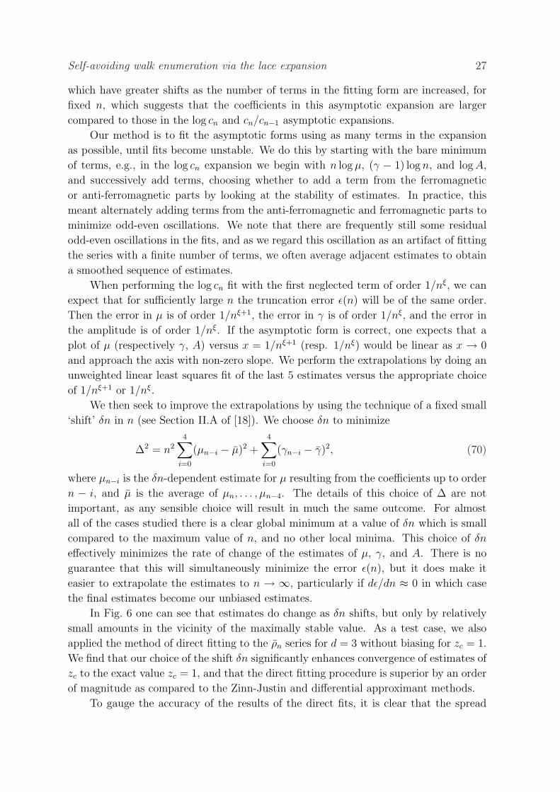
In Fig. 6 one can see that estimates do change as δn shifts, but only by relatively
small amounts in the vicinity of the maximally stable value. As a test case, we also
applied the method of direct fitting to the ρn series for d = 3 without biasing for zc = 1.
We find that our choice of the shift δn significantly enhances convergence of estimates of
zc to the exact value zc = 1, and that the direct fitting procedure is superior by an order
of magnitude as compared to the Zinn-Justin and differential approximant methods.
To gauge the accuracy of the results of the direct fits, it is clear that the spread
Self-avoiding walk enumeration via the lace expansion 28
1.1564
1.1566
1.1568
1.157
1.1572
1.1574
0 0.002 0.004 0.006 0.008 0.01
n-3/2
γ
δn=0.39
δn=0.49
δn=0.59
δn=0.69
δn=0.79
δn=0.89
δn=0.99
Figure 6. Estimates for γ for d = 3 from fit of log cn with highest-order terms q1, r2for different values of δn, where δn = 0.69 minimizes ∆2.
among estimates of the same order is a lower bound on the uncertainty. If estimates
from the fits are converging sufficiently rapidly as the order is increased, then the jump
from the second highest-order fit to the highest-order fit may give some idea of the size
of the uncertainty. Therefore the recipe we use to analyze series via this procedure is
to find the highest-order stable fits, exclude those fits which appear to be converging
anomalously slowly, and take the mean of the reliable fits as our central estimate. We
then calculate the mean of the jumps from the second highest-order fits to the highest-
order fits, and quote this value to give some idea of the accuracy of our central estimate.
We do not claim that this is a rigorous procedure, nor that this should in any way be
interpreted as a statistical error estimate.
6. Analysis of series: results
In this section, we analyze the series for cn, ρn, ρn and pn, using the methods discussed
in Section 5. We first consider the important case d = 3 at length, then d ≥ 4, and
finally we analyze the 1/d expansion for µ. We used multiple precision floating point
computations via the GMP bignum library, to ensure numerical robustness.
6.1. Analysis for d = 3
We first analyze the series on the cubic lattice Z3 for cn, for ρn and ρn, and for pn.
6.1.1. Analysis of the series cn
The method of differential approximants. In Table 1, we give estimates for µ and γ
from second- and third-order unbiased differential approximants, where the value in
parentheses is the standard deviation of the estimates after we have pruned away outliers.

Self-avoiding walk enumeration via the lace expansion 29
Table 1. Differential approximants for cn.
Second-order DA Third-order DA
N µ γ U/T µ γ U/T
21 4.683846(51) 1.16198(47) 35/45 4.683831(56) 1.16213(53) 76/87
22 4.683920(43) 1.16125(47) 40/44 4.68387(11) 1.1614(11) 88/99
23 4.683921(22) 1.16119(34) 41/44 4.683904(45) 1.16131(59) 76/104
24 4.683927(16) 1.16112(25) 37/45 4.683890(38) 1.16157(39) 74/107
25 4.683931(58) 1.16092(97) 38/44 4.683937(69) 1.1606(11) 76/113
26 4.683974(33) 1.16024(78) 42/44 4.684017(41) 1.1590(12) 98/116
27 4.683999(55) 1.1594(14) 40/45 4.684017(32) 1.15907(96) 90/114
28 4.683997(34) 1.15973(94) 39/44 4.684022(13) 1.15901(47) 96/111
29 4.684038(21) 1.15842(86) 37/44 4.6840182(45) 1.15916(16) 90/114
30 4.684019(33) 1.1591(15) 44/45 4.6840224(53) 1.15900(21) 110/116
The number of approximants utilized to obtain the estimates is U , while T is the total
number of approximants including the excluded outliers. The results of Table 1 reveal
that the estimates for µ (γ) still have an upwards (downwards) trend as N increases.
The third-order approximants suggest a value µ in the vicinity of 4.68402 and γ near
1.1590, but given that the second-order approximants have not settled down we believe
this apparent convergence to be spurious, and expect that systematic shifts in µ and γ
will continue.
The method of Zinn-Justin. We suppose first that θ = 0.5; later we will see how
estimates change under variation in θ. Application of the method of Zinn-Justin gives
estimates of µ = 4.684024 and µ = 4.684033 for the odd and even subsequences
respectively, both of which are slowly increasing with N . The exponent estimates are
γ = 1.15704 and γ = 1.15703, both estimates slowly decreasing with N .
The method of direct fitting. For direct fitting, we found for each form that the highest-
order fits for which smoothly changing values were observed for all coefficients have
highest-order terms q1 and r2. We again suppose first that θ = 0.5, and consider
alternate possibilities for θ afterward.
Tables 2–4 show the highest-order fits for log cn, cn/cn−1, and cn/cn−2. All estimates
are extremely stable, suggesting that the fitting forms of Equations (67)–(69) are
basically correct. In particular, we regard the r2 estimates in Table 3 as stable because
the absolute values of successive estimates are similar and close to zero, and it is absolute
rather than relative changes in value that are important, as coefficients may be genuinely
close to zero.
We extrapolate the estimates from Tables 2–4, as well as the estimates from the

Self-avoiding walk enumeration via the lace expansion 30
Table 2. Smoothed coefficients in asymptotic expansion of log cn with θ = 0.5.
N µ γ A q0 q1 r0 r1 r2
21 4.6840569 1.15653 1.21859 -0.0693 0.0304 -0.0641 -0.0337 0.0211
22 4.6840526 1.15667 1.21773 -0.0676 0.0288 -0.0643 -0.0316 0.0166
23 4.6840343 1.15709 1.21520 -0.0628 0.0250 -0.0645 -0.0299 0.0131
24 4.6840385 1.15699 1.21577 -0.0639 0.0259 -0.0646 -0.0292 0.0113
25 4.6840356 1.15707 1.21534 -0.0630 0.0252 -0.0646 -0.0287 0.0102
26 4.6840364 1.15705 1.21545 -0.0632 0.0253 -0.0647 -0.0283 0.0094
27 4.6840371 1.15702 1.21562 -0.0636 0.0257 -0.0647 -0.0279 0.0085
28 4.6840375 1.15701 1.21566 -0.0637 0.0257 -0.0648 -0.0275 0.0075
29 4.6840376 1.15701 1.21571 -0.0638 0.0259 -0.0648 -0.0271 0.0064
30 4.6840381 1.15699 1.21579 -0.0639 0.0260 -0.0648 -0.0267 0.0053
Table 3. Smoothed coefficients in asymptotic expansion of cn/cn−1 with θ = 0.5.
N µ γ q0 q1 r0 r1 r2
21 4.6840409 1.15707 0.0307 -0.0279 -0.1292 -0.0559 0.0168
22 4.6840379 1.15717 0.0301 -0.0268 -0.1295 -0.0527 0.0101
23 4.6840230 1.15751 0.0281 -0.0237 -0.1298 -0.0503 0.0049
24 4.6840280 1.15739 0.0288 -0.0248 -0.1299 -0.0495 0.0030
25 4.6840272 1.15741 0.0287 -0.0247 -0.1300 -0.0491 0.0023
26 4.6840287 1.15737 0.0290 -0.0251 -0.1300 -0.0490 0.0020
27 4.6840308 1.15731 0.0294 -0.0258 -0.1300 -0.0488 0.0014
28 4.6840316 1.15728 0.0295 -0.0261 -0.1300 -0.0484 0.0005
29 4.6840326 1.15725 0.0298 -0.0266 -0.1301 -0.0480 -0.0006
30 4.6840335 1.15722 0.0299 -0.0269 -0.1301 -0.0475 -0.0017
lower-order fits. This information is summarized in Table 5, and shown graphically for
the highest-order fits in Figures 7–9. The most important features of Table 5 are that
the estimates for the log cn and cn/cn−1 fits seem to be converging quite rapidly, as the
jumps from the q0, r1 to the q1, r2 fits appear quite small. The final jumps for the
cn/cn−2 fit are somewhat larger, which suggests that the coefficients in the asymptotic
expansion for cn/cn−2 are perhaps larger; if the coefficients are uniformly larger than
those for the other fits then we would expect the cn/cn−2 estimates to be less accurate.
We exclude the cn/cn−2 fits, and follow the procedure of Section 5.3 to obtain the
estimates in Table 13 for µ, γ, and A.
We can also obtain a range of estimates for γ by exploiting the approximately linear
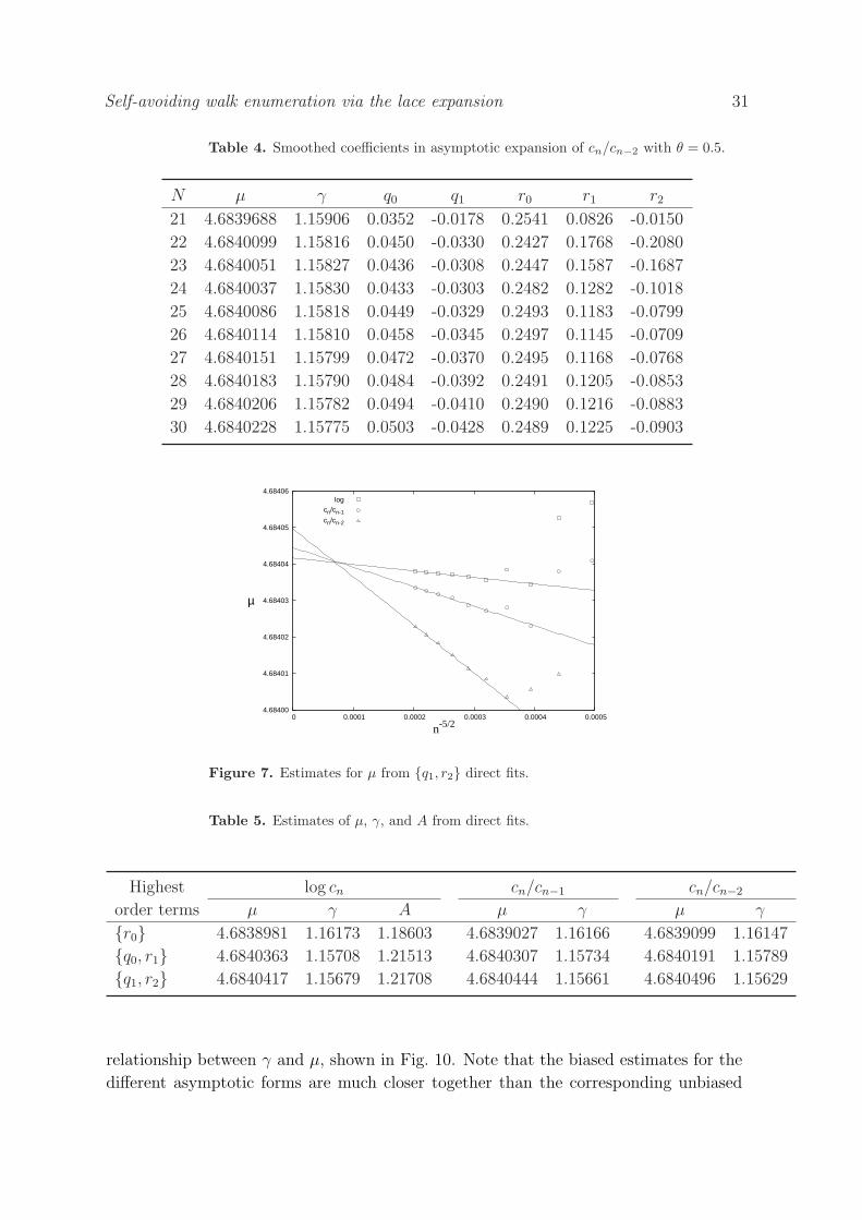
Self-avoiding walk enumeration via the lace expansion 31
Table 4. Smoothed coefficients in asymptotic expansion of cn/cn−2 with θ = 0.5.
N µ γ q0 q1 r0 r1 r2
21 4.6839688 1.15906 0.0352 -0.0178 0.2541 0.0826 -0.0150
22 4.6840099 1.15816 0.0450 -0.0330 0.2427 0.1768 -0.2080
23 4.6840051 1.15827 0.0436 -0.0308 0.2447 0.1587 -0.1687
24 4.6840037 1.15830 0.0433 -0.0303 0.2482 0.1282 -0.1018
25 4.6840086 1.15818 0.0449 -0.0329 0.2493 0.1183 -0.0799
26 4.6840114 1.15810 0.0458 -0.0345 0.2497 0.1145 -0.0709
27 4.6840151 1.15799 0.0472 -0.0370 0.2495 0.1168 -0.0768
28 4.6840183 1.15790 0.0484 -0.0392 0.2491 0.1205 -0.0853
29 4.6840206 1.15782 0.0494 -0.0410 0.2490 0.1216 -0.0883
30 4.6840228 1.15775 0.0503 -0.0428 0.2489 0.1225 -0.0903
4.68406
4.68405
4.68404
4.68403
4.68402
4.68401
4.68400 0 0.0001 0.0002 0.0003 0.0004 0.0005
n-5/2
µ
logcn/cn-1
cn/cn-2
Figure 7. Estimates for µ from q1, r2 direct fits.
Table 5. Estimates of µ, γ, and A from direct fits.
Highest log cn cn/cn−1 cn/cn−2
order terms µ γ A µ γ µ γ
r0 4.6838981 1.16173 1.18603 4.6839027 1.16166 4.6839099 1.16147
q0, r1 4.6840363 1.15708 1.21513 4.6840307 1.15734 4.6840191 1.15789
q1, r2 4.6840417 1.15679 1.21708 4.6840444 1.15661 4.6840496 1.15629
relationship between γ and µ, shown in Fig. 10. Note that the biased estimates for the
different asymptotic forms are much closer together than the corresponding unbiased
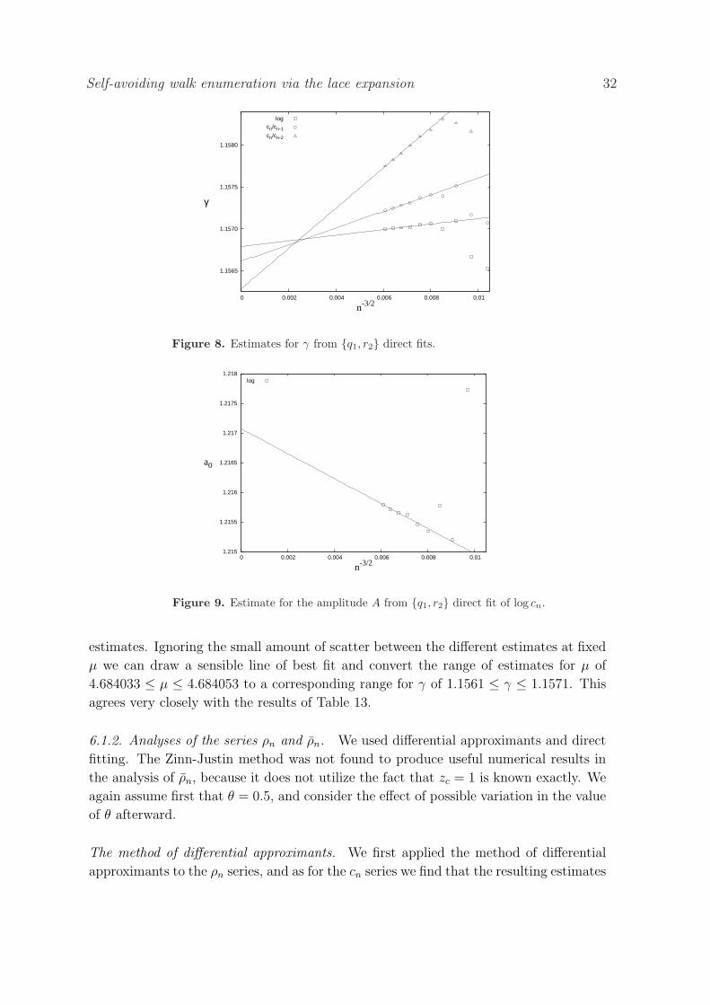
Self-avoiding walk enumeration via the lace expansion 32
1.1580
1.1575
1.1570
1.1565
0 0.002 0.004 0.006 0.008 0.01
n-3/2
γ
logcn/cn-1
cn/cn-2
Figure 8. Estimates for γ from q1, r2 direct fits.
1.215
1.2155
1.216
1.2165
1.217
1.2175
1.218
0 0.002 0.004 0.006 0.008 0.01
n-3/2
a0
log
Figure 9. Estimate for the amplitude A from q1, r2 direct fit of log cn.
estimates. Ignoring the small amount of scatter between the different estimates at fixed
µ we can draw a sensible line of best fit and convert the range of estimates for µ of
4.684033 ≤ µ ≤ 4.684053 to a corresponding range for γ of 1.1561 ≤ γ ≤ 1.1571. This
agrees very closely with the results of Table 13.
6.1.2. Analyses of the series ρn and ρn. We used differential approximants and direct
fitting. The Zinn-Justin method was not found to produce useful numerical results in
the analysis of ρn, because it does not utilize the fact that zc = 1 is known exactly. We
again assume first that θ = 0.5, and consider the effect of possible variation in the value
of θ afterward.
The method of differential approximants. We first applied the method of differential
approximants to the ρn series, and as for the cn series we find that the resulting estimates
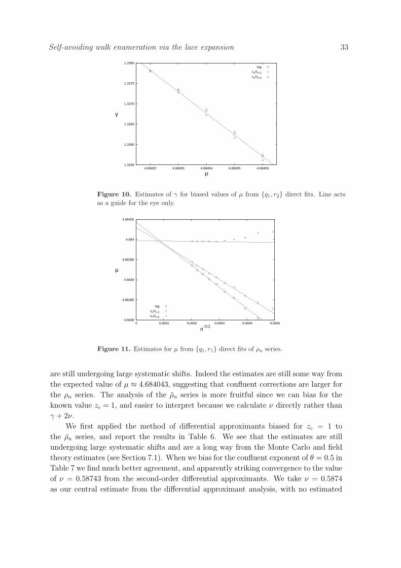
Self-avoiding walk enumeration via the lace expansion 33
1.1580
1.1575
1.1570
1.1565
1.1560
1.15554.684064.684054.684044.684034.68402
µ
γ
logcn/cn-1
cn/cn-2
Figure 10. Estimates of γ for biased values of µ from q1, r2 direct fits. Line actsas a guide for the eye only.
4.6838
4.68385
4.6839
4.68395
4.684
4.68405
0 0.0001 0.0002 0.0003 0.0004 0.0005
n-5/2
µ
logcn/cn-1
cn/cn-2
Figure 11. Estimates for µ from q1, r1 direct fits of ρn series.
are still undergoing large systematic shifts. Indeed the estimates are still some way from
the expected value of µ ≈ 4.684043, suggesting that confluent corrections are larger for
the ρn series. The analysis of the ρn series is more fruitful since we can bias for the
known value zc = 1, and easier to interpret because we calculate ν directly rather than
γ + 2ν.
We first applied the method of differential approximants biased for zc = 1 to
the ρn series, and report the results in Table 6. We see that the estimates are still
undergoing large systematic shifts and are a long way from the Monte Carlo and field
theory estimates (see Section 7.1). When we bias for the confluent exponent of θ = 0.5 in
Table 7 we find much better agreement, and apparently striking convergence to the value
of ν = 0.58743 from the second-order differential approximants. We take ν = 0.5874
as our central estimate from the differential approximant analysis, with no estimated
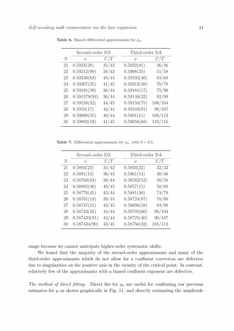
Self-avoiding walk enumeration via the lace expansion 34
Table 6. Biased differential approximants for ρn.
Second-order DA Third-order DA
N ν U/T ν U/T
21 0.5933(28) 35/42 0.5922(81) 46/46
22 0.59212(99) 38/43 0.5908(35) 51/58
23 0.59230(63) 43/44 0.59192(46) 63/68
24 0.59207(35) 41/45 0.59212(38) 70/78
25 0.59191(39) 36/44 0.59181(17) 75/90
26 0.591579(94) 36/44 0.59146(32) 93/99
27 0.59138(32) 44/45 0.59158(75) 100/104
28 0.5910(17) 42/44 0.59103(91) 98/107
29 0.59080(45) 40/44 0.5901(11) 108/113
30 0.59092(59) 41/45 0.59058(88) 110/116
Table 7. Differential approximants for ρn, with θ = 0.5.
Second-order DA Third-order DA
N ν U/T ν U/T
21 0.5893(23) 35/42 0.5850(22) 32/33
22 0.5881(14) 36/43 0.5861(14) 40/46
23 0.58768(93) 38/44 0.58582(52) 50/58
24 0.58805(40) 40/45 0.5857(15) 58/68
25 0.58776(45) 43/44 0.5881(40) 74/78
26 0.58761(18) 39/44 0.58724(87) 78/90
27 0.58747(21) 43/45 0.58698(58) 93/99
28 0.58743(42) 44/44 0.58702(66) 98/104
29 0.587433(91) 42/44 0.58725(40) 90/107
30 0.587434(90) 43/45 0.58756(32) 105/113
range because we cannot anticipate higher-order systematic shifts.
We found that the majority of the second-order approximants and many of the
third-order approximants which do not allow for a confluent correction are defective
due to singularities on the positive axis in the vicinity of the critical point. In contrast,
relatively few of the approximants with a biased confluent exponent are defective.
The method of direct fitting. Direct fits for ρn are useful for confirming our previous
estimates for µ as shown graphically in Fig. 11, and directly estimating the amplitude
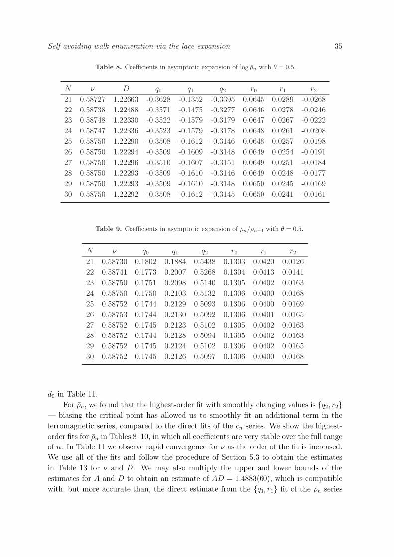
Self-avoiding walk enumeration via the lace expansion 35
Table 8. Coefficients in asymptotic expansion of log ρn with θ = 0.5.
N ν D q0 q1 q2 r0 r1 r2
21 0.58727 1.22663 -0.3628 -0.1352 -0.3395 0.0645 0.0289 -0.0268
22 0.58738 1.22488 -0.3571 -0.1475 -0.3277 0.0646 0.0278 -0.0246
23 0.58748 1.22330 -0.3522 -0.1579 -0.3179 0.0647 0.0267 -0.0222
24 0.58747 1.22336 -0.3523 -0.1579 -0.3178 0.0648 0.0261 -0.0208
25 0.58750 1.22290 -0.3508 -0.1612 -0.3146 0.0648 0.0257 -0.0198
26 0.58750 1.22294 -0.3509 -0.1609 -0.3148 0.0649 0.0254 -0.0191
27 0.58750 1.22296 -0.3510 -0.1607 -0.3151 0.0649 0.0251 -0.0184
28 0.58750 1.22293 -0.3509 -0.1610 -0.3146 0.0649 0.0248 -0.0177
29 0.58750 1.22293 -0.3509 -0.1610 -0.3148 0.0650 0.0245 -0.0169
30 0.58750 1.22292 -0.3508 -0.1612 -0.3145 0.0650 0.0241 -0.0161
Table 9. Coefficients in asymptotic expansion of ρn/ρn−1 with θ = 0.5.
N ν q0 q1 q2 r0 r1 r2
21 0.58730 0.1802 0.1884 0.5438 0.1303 0.0420 0.0126
22 0.58741 0.1773 0.2007 0.5268 0.1304 0.0413 0.0141
23 0.58750 0.1751 0.2098 0.5140 0.1305 0.0402 0.0163
24 0.58750 0.1750 0.2103 0.5132 0.1306 0.0400 0.0168
25 0.58752 0.1744 0.2129 0.5093 0.1306 0.0400 0.0169
26 0.58753 0.1744 0.2130 0.5092 0.1306 0.0401 0.0165
27 0.58752 0.1745 0.2123 0.5102 0.1305 0.0402 0.0163
28 0.58752 0.1744 0.2128 0.5094 0.1305 0.0402 0.0163
29 0.58752 0.1745 0.2124 0.5102 0.1306 0.0402 0.0165
30 0.58752 0.1745 0.2126 0.5097 0.1306 0.0400 0.0168
d0 in Table 11.
For ρn, we found that the highest-order fit with smoothly changing values is q2, r2— biasing the critical point has allowed us to smoothly fit an additional term in the
ferromagnetic series, compared to the direct fits of the cn series. We show the highest-
order fits for ρn in Tables 8–10, in which all coefficients are very stable over the full range
of n. In Table 11 we observe rapid convergence for ν as the order of the fit is increased.
We use all of the fits and follow the procedure of Section 5.3 to obtain the estimates
in Table 13 for ν and D. We may also multiply the upper and lower bounds of the
estimates for A and D to obtain an estimate of AD = 1.4883(60), which is compatible
with, but more accurate than, the direct estimate from the q1, r1 fit of the ρn series
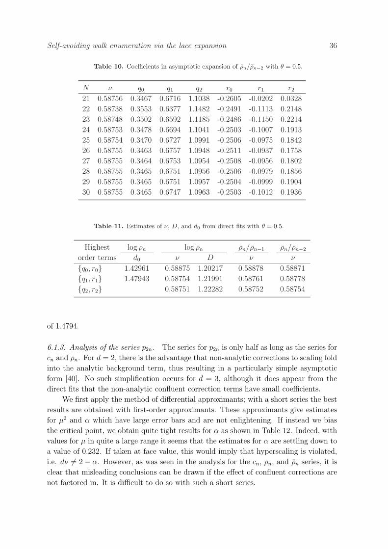
Self-avoiding walk enumeration via the lace expansion 36
Table 10. Coefficients in asymptotic expansion of ρn/ρn−2 with θ = 0.5.
N ν q0 q1 q2 r0 r1 r2
21 0.58756 0.3467 0.6716 1.1038 -0.2605 -0.0202 0.0328
22 0.58738 0.3553 0.6377 1.1482 -0.2491 -0.1113 0.2148
23 0.58748 0.3502 0.6592 1.1185 -0.2486 -0.1150 0.2214
24 0.58753 0.3478 0.6694 1.1041 -0.2503 -0.1007 0.1913
25 0.58754 0.3470 0.6727 1.0991 -0.2506 -0.0975 0.1842
26 0.58755 0.3463 0.6757 1.0948 -0.2511 -0.0937 0.1758
27 0.58755 0.3464 0.6753 1.0954 -0.2508 -0.0956 0.1802
28 0.58755 0.3465 0.6751 1.0956 -0.2506 -0.0979 0.1856
29 0.58755 0.3465 0.6751 1.0957 -0.2504 -0.0999 0.1904
30 0.58755 0.3465 0.6747 1.0963 -0.2503 -0.1012 0.1936
Table 11. Estimates of ν, D, and d0 from direct fits with θ = 0.5.
Highest log ρn log ρn ρn/ρn−1 ρn/ρn−2
order terms d0 ν D ν ν
q0, r0 1.42961 0.58875 1.20217 0.58878 0.58871
q1, r1 1.47943 0.58754 1.21991 0.58761 0.58778
q2, r2 0.58751 1.22282 0.58752 0.58754
of 1.4794.
6.1.3. Analysis of the series p2n. The series for p2n is only half as long as the series for
cn and ρn. For d = 2, there is the advantage that non-analytic corrections to scaling fold
into the analytic background term, thus resulting in a particularly simple asymptotic
form [40]. No such simplification occurs for d = 3, although it does appear from the
direct fits that the non-analytic confluent correction terms have small coefficients.
We first apply the method of differential approximants; with a short series the best
results are obtained with first-order approximants. These approximants give estimates
for µ2 and α which have large error bars and are not enlightening. If instead we bias
the critical point, we obtain quite tight results for α as shown in Table 12. Indeed, with
values for µ in quite a large range it seems that the estimates for α are settling down to
a value of 0.232. If taken at face value, this would imply that hyperscaling is violated,
i.e. dν 6= 2− α. However, as was seen in the analysis for the cn, ρn, and ρn series, it is
clear that misleading conclusions can be drawn if the effect of confluent corrections are
not factored in. It is difficult to do so with such a short series.

Self-avoiding walk enumeration via the lace expansion 37
Table 12. Biased estimates for α from first-order DA.
µ = 4.68402 µ = 4.68404 µ = 4.68406
N α U/T α U/T α U/T
24 0.242(28) 10/10 0.241(28) 10/10 0.241(28) 10/10
26 0.230(11) 13/13 0.229(11) 13/13 0.229(11) 13/13
28 0.2325(16) 13/14 0.2321(16) 13/14 0.2317(16) 13/14
30 0.23251(56) 15/15 0.23208(54) 15/15 0.23166(53) 15/15
32 0.23251(18) 15/15 0.23202(16) 15/15 0.23153(13) 15/15
Table 13. Estimates of parameters for d = 3 from direct fits with θ = 0.5. Theseare intermediate results which do not yet take into account variation in θ, a dominantsource of uncertainty.
µ γ ν A D
4.6840431(96) 1.15670(51) 0.58752(12) 1.2171(20) 1.2228(29)
Direct fits are also not revealing: it is not possible to get good unbiased estimates of
µ2 and α; when a biased value of µ is used it is possible to fit for a confluent correction
with exponent θ, and an analytic correction, but the convergence is not very good and
we do not quote these results here. They suggest that α is in the range of 0.23− 0.24,
consistent with hyperscaling, but without a longer series not much more can be said
with confidence.
6.1.4. Effect of variation in θ. Table 31 of [55] reports a wide range of estimates for
θ, from a low of 0.46–0.50 from various field theory estimates, to a high of 0.56(3) from
the Monte Carlo estimate of [45]. It is therefore important that we repeat the above
analysis to quantify the dependence on θ of our estimates for µ, γ, A, ν, D.
The results for µ, γ, ν are shown in Figs. 12–14, with the central estimates given the
label ‘Best’. It is apparent from the figures that the estimates depend approximately
linearly on the value of θ used, and we observed similar linear behavior for A and D.
Our method of producing error estimates gives comparable results as θ is varied, and
given that this error estimate is subjective in any case we take the uncertainties to be
constant. The results can be succinctly summarized by the linear least squares fits to
the central estimates:
µ(θ) = 4.6840431− 0.0000394(θ − 0.5)± 0.00001 (71)
γ(θ) = 1.156690 + 0.006779(θ − 0.5)± 0.0005 (72)
A(θ) = 1.21723− 0.06379(θ − 0.5)± 0.002 (73)

Self-avoiding walk enumeration via the lace expansion 38
4.68405
4.68404
4.68403
0.46 0.48 0.5 0.52 0.54 0.56
θ
µ
ZJ
logcn/cn-1
cn/cn-2
Best
Figure 12. Estimates for µ from q1, r2 direct fits and the method of Zinn-Justin,plotted versus θ. Line of best fit to the central estimates (‘Best’) is also shown.
1.156
1.1562
1.1564
1.1566
1.1568
1.157
1.1572
1.1574
1.1576
0.46 0.48 0.5 0.52 0.54 0.56
θ
γ
ZJ
logcn/cn-1
cn/cn-2
Best
Figure 13. Estimates for γ from q1, r2 direct fits and the method of Zinn-Justin,plotted versus θ. Line of best fit to the central estimates (‘Best’) is also shown.
ν(θ) = 0.587506 + 0.008324(θ − 0.5)± 0.00012 (74)
D(θ) = 1.22330− 0.19743(θ − 0.5)± 0.003. (75)
We show these lines on Figs. 12–14, and it is clear that the fit is excellent in each case.
If we adopt a range of θ1 ≤ θ ≤ θ2, we then convert this to a range, e.g., for µ of
µ(θ2)− 0.00001 ≤ µ ≤ µ(θ1) + 0.00001.
We note in passing that the ‘shift’ δn is insensitive to changes in θ, for example in
the fit for log cn with corrections to order 1/n, δn only changes from 0.709 to 0.715 as
θ is varied from 0.47 to 0.53. For this reason we can use a single value of δn.

Self-avoiding walk enumeration via the lace expansion 39
0.587
0.5872
0.5874
0.5876
0.5878
0.588
0.5882
0.46 0.48 0.5 0.52 0.54 0.56
θ
ν
logcn/cn-1
cn/cn-2
Best
Figure 14. Estimates for ν from q2, r2 fits plotted versus θ. Line of best fit to thecentral estimates (‘Best’) is also shown.
6.2. Analysis for d = 4
The series in d = 4 require particular attention because of the logarithmic corrections:
cn ∼ Aµn (log n)1/4 , ρn ∼ Dn(log n)1/4. (76)
Confluent corrections of the form log log n/ log n have been elucidated by Duplantier
[13].
The method of differential approximants. Unbiased differential approximants cannot
take into account the logarithmic confluent correction, but nevertheless give useful
estimates. Second- and third-order inhomogeneous approximants give µ = 6.7737 ↑(trending upwards), and γ = 1.046 ↓ (trending downwards). Biasing γ = 1 by
performing a linear fit in the plot of zc versus γ, as described below Eqn. (57), gives worse
results, suggesting µ = 6.777 ↓; this is probably because the unbiased approximants take
into account the leading logarithmic correction via an effective exponent. Nonetheless,
it appears that the unbiased and biased estimates bracket the correct value of µ (we find
this to be the case for dimensions 4 ≤ d ≤ 7), and so we take the mean and estimate
the uncertainty from the spread of the two estimates.
The method of Zinn-Justin. Naive application of this method, which does not take into
account the logarithmic confluent correction, gives µ = 6.77363 ↑ if we take θ = 1 as
indicated by the direct fits.
The method of direct fitting. Direct fitting works extremely well when the logarithmic
correction is taken into account. This results, for example, in a log log term for the
log cn fitting form, and works much better when treated as an effective exponent, rather
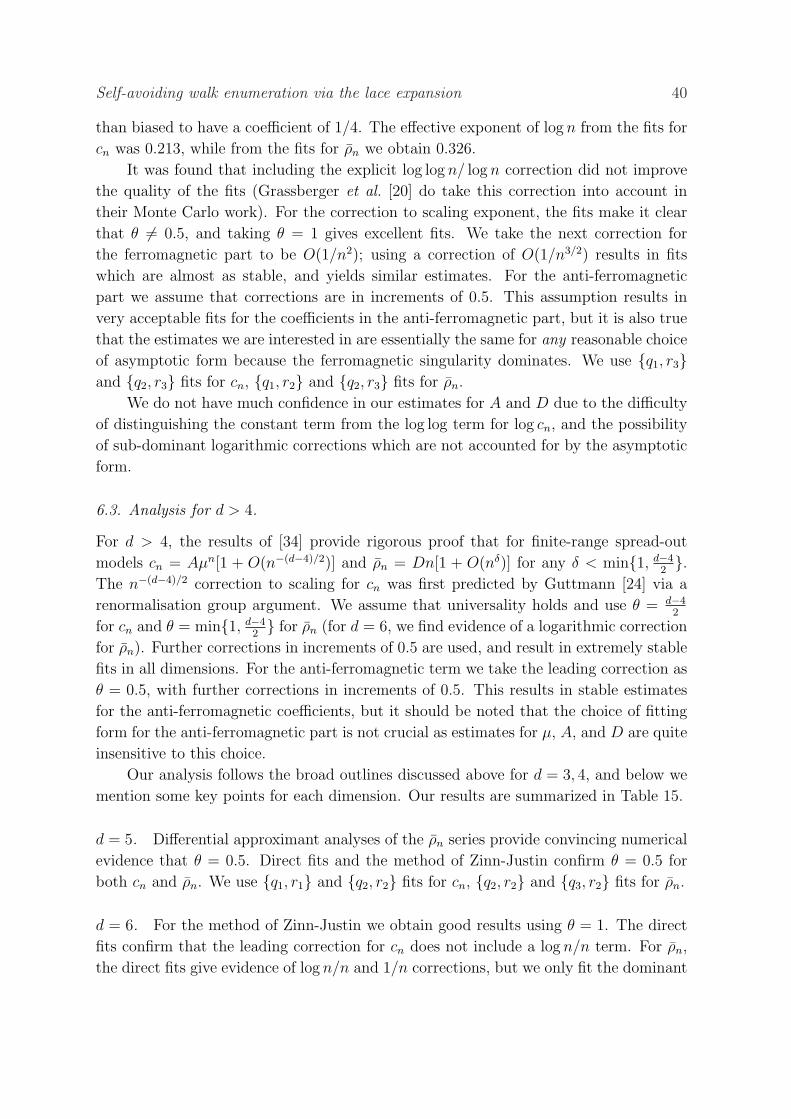
Self-avoiding walk enumeration via the lace expansion 40
than biased to have a coefficient of 1/4. The effective exponent of log n from the fits for
cn was 0.213, while from the fits for ρn we obtain 0.326.
It was found that including the explicit log log n/ log n correction did not improve
the quality of the fits (Grassberger et al. [20] do take this correction into account in
their Monte Carlo work). For the correction to scaling exponent, the fits make it clear
that θ 6= 0.5, and taking θ = 1 gives excellent fits. We take the next correction for
the ferromagnetic part to be O(1/n2); using a correction of O(1/n3/2) results in fits
which are almost as stable, and yields similar estimates. For the anti-ferromagnetic
part we assume that corrections are in increments of 0.5. This assumption results in
very acceptable fits for the coefficients in the anti-ferromagnetic part, but it is also true
that the estimates we are interested in are essentially the same for any reasonable choice
of asymptotic form because the ferromagnetic singularity dominates. We use q1, r3and q2, r3 fits for cn, q1, r2 and q2, r3 fits for ρn.
We do not have much confidence in our estimates for A and D due to the difficulty
of distinguishing the constant term from the log log term for log cn, and the possibility
of sub-dominant logarithmic corrections which are not accounted for by the asymptotic
form.
6.3. Analysis for d > 4.
For d > 4, the results of [34] provide rigorous proof that for finite-range spread-out
models cn = Aµn[1 + O(n−(d−4)/2)] and ρn = Dn[1 + O(nδ)] for any δ < min1, d−42.
The n−(d−4)/2 correction to scaling for cn was first predicted by Guttmann [24] via a
renormalisation group argument. We assume that universality holds and use θ = d−42
for cn and θ = min1, d−42 for ρn (for d = 6, we find evidence of a logarithmic correction
for ρn). Further corrections in increments of 0.5 are used, and result in extremely stable
fits in all dimensions. For the anti-ferromagnetic term we take the leading correction as
θ = 0.5, with further corrections in increments of 0.5. This results in stable estimates
for the anti-ferromagnetic coefficients, but it should be noted that the choice of fitting
form for the anti-ferromagnetic part is not crucial as estimates for µ, A, and D are quite
insensitive to this choice.
Our analysis follows the broad outlines discussed above for d = 3, 4, and below we
mention some key points for each dimension. Our results are summarized in Table 15.
d = 5. Differential approximant analyses of the ρn series provide convincing numerical
evidence that θ = 0.5. Direct fits and the method of Zinn-Justin confirm θ = 0.5 for
both cn and ρn. We use q1, r1 and q2, r2 fits for cn, q2, r2 and q3, r2 fits for ρn.
d = 6. For the method of Zinn-Justin we obtain good results using θ = 1. The direct
fits confirm that the leading correction for cn does not include a log n/n term. For ρn,
the direct fits give evidence of log n/n and 1/n corrections, but we only fit the dominant
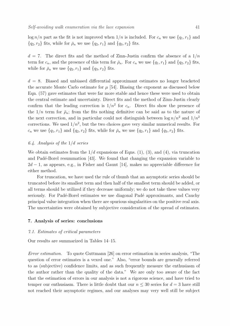
Self-avoiding walk enumeration via the lace expansion 41
log n/n part as the fit is not improved when 1/n is included. For cn we use q1, r1 and
q2, r2 fits, while for ρn we use q2, r1 and q3, r2 fits.
d = 7. The direct fits and the method of Zinn-Justin confirm the absence of a 1/n
term for cn, and the presence of this term for ρn. For cn we use q1, r1 and q2, r2 fits,
while for ρn we use q2, r1 and q3, r2 fits.
d = 8. Biased and unbiased differential approximant estimates no longer bracketed
the accurate Monte Carlo estimate for µ [54]. Biasing the exponent as discussed below
Eqn. (57) gave estimates that were far more stable and hence these were used to obtain
the central estimate and uncertainty. Direct fits and the method of Zinn-Justin clearly
confirm that the leading correction is 1/n2 for cn. Direct fits show the presence of
the 1/n term for ρn; from the fits nothing definitive can be said as to the nature of
the next correction, and in particular could not distinguish between log n/n2 and 1/n2
corrections. We used 1/n2, but the two choices gave very similar numerical results. For
cn we use q1, r1 and q2, r2 fits, while for ρn we use q2, r1 and q3, r2 fits.
6.4. Analysis of the 1/d series
We obtain estimates from the 1/d expansions of Eqns. (1), (3), and (4), via truncation
and Pade-Borel resummation [43]. We found that changing the expansion variable to
2d − 1, as appears, e.g., in Fisher and Gaunt [14], makes no appreciable difference for
either method.
For truncation, we have used the rule of thumb that an asymptotic series should be
truncated before its smallest term and then half of the smallest term should be added, or
all terms should be utilized if they decrease uniformly; we do not take these values very
seriously. For Pade-Borel estimates we use diagonal Pade approximants, and Cauchy
principal value integration when there are spurious singularities on the positive real axis.
The uncertainties were obtained by subjective consideration of the spread of estimates.
7. Analysis of series: conclusions
7.1. Estimates of critical parameters
Our results are summarized in Tables 14–15.
Error estimation. To quote Guttmann [26] on error estimation in series analysis, “The
question of error estimates is a vexed one.” Also, “error bounds are generally referred
to as (subjective) confidence limits, and as such frequently measure the enthusiasm of
the author rather than the quality of the data.” We are only too aware of the fact
that the estimation of errors in our analysis is not a rigorous science, and have tried to
temper our enthusiasm. There is little doubt that our n ≤ 30 series for d = 3 have still
not reached their asymptotic regimes, and our analyses may very well still be subject
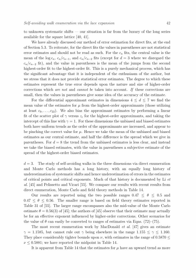
Self-avoiding walk enumeration via the lace expansion 42
to unknown systematic shifts — our situation is far from the luxury of the long series
available for the square lattice [40, 41].
We have already discussed our method of error estimation for direct fits, at the end
of Section 5.3. To reiterate, for the direct fits the values in parentheses are not statistical
error estimates and should not be read as such. For the cn fits, the central value is the
mean of the log cn, cn/cn−1, and cn/cn−2 fits (except for d = 3 where we disregard the
cn/cn−2 fit), and the value in parentheses is the mean of the jumps from the second
highest-order fit to the highest-order fit. This is a purely mechanical process, which has
the significant advantage that it is independent of the enthusiasm of the author, but
we stress that it does not provide statistical error estimates. The degree to which these
estimates represent the true error depends upon the nature and size of higher-order
corrections which are not and cannot be taken into account. If these corrections are
small, then the values in parentheses give some idea of the accuracy of the estimate.
For the differential approximant estimates in dimensions 4 ≤ d ≤ 7 we find the
mean value of the estimates for µ from the highest-order approximants (those utilizing
at least c0, . . . , c22). We also bias the approximant estimates by performing a linear
fit of the scatter plot of γ versus zc for the highest-order approximants, and taking the
intercept of this line with γ = 1. For these dimensions the unbiased and biased estimates
both have uniform trends as the order of the approximants are increased, and appear to
be pinching the correct value for µ. Hence we take the mean of the unbiased and biased
estimates as our central estimate, and half the difference is the spread which we give in
parentheses. For d = 8 the trend from the unbiased estimates is less clear, and instead
we take the biased estimates, with the value in parentheses a subjective estimate of the
spread of the highest-order biased estimates.
d = 3. The study of self-avoiding walks in the three dimensions via direct enumeration
and Monte Carlo methods has a long history, with an equally long history of
underestimation of systematic shifts and hence underestimation of errors in the estimates
of critical points and critical exponents. Much of that history is documented by Li et
al. [45] and Pelissetto and Vicari [55]. We compare our results with recent results from
direct enumeration, Monte Carlo and field theory methods in Table 14.
Our results are reported using the two possible ranges 0.47 ≤ θ ≤ 0.5 and
0.47 ≤ θ ≤ 0.56. The smaller range is based on field theory estimates reported in
Table 31 of [55]. The larger range encompasses also the mid-value of the Monte Carlo
estimate θ = 0.56(3) of [45]; the authors of [45] observe that their estimate may actually
be for an effective exponent influenced by higher-order corrections. Other scenarios for
the value of θ can easily be converted to ranges of estimates via Eqns. (72)–(75).
The most recent enumeration work by MacDonald et al. [47] gives an estimate
γ = 1.1585, but cannot rule out γ being elsewhere in the range 1.155 ≤ γ ≤ 1.160.
They place considerably tighter bounds upon ν, with estimates in the range of 0.5870 ≤ν ≤ 0.5881; we have reported the midpoint in Table 14.
It is apparent from Table 14 that the estimates for µ have an upward trend as more
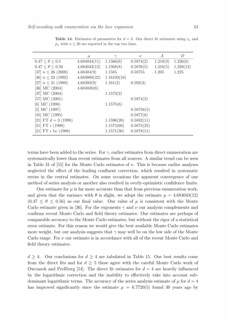
Self-avoiding walk enumeration via the lace expansion 43
Table 14. Estimates of parameters for d = 3. Our direct fit estimates using cn andρn with n ≤ 30 are reported in the top two lines.
µ γ ν A D
0.47 ≤ θ ≤ 0.5 4.684044(11) 1.1566(6) 0.5874(2) 1.218(3) 1.226(6)0.47 ≤ θ ≤ 0.56 4.684043(12) 1.1568(8) 0.5876(5) 1.216(5) 1.220(12)[47] n ≤ 26 (2000) 4.68404(9) 1.1585 0.58755 1.205 1.225[46] n ≤ 23 (1992) 4.683869(22) 1.16193(10)[27] n ≤ 21 (1989) 4.68393(9) 1.161(2) 0.592(3)[36] MC (2004) 4.684038(6)[37] MC (2004) 1.1573(2)[57] MC (2001) 0.5874(2)[6] MC (1998) 1.1575(6)[2] MC (1997) 0.58756(5)[45] MC (1995) 0.5877(6)[21] FT d = 3 (1998) 1.1596(20) 0.5882(11)[21] FT ε (1998) 1.1575(60) 0.5875(25)[21] FT ε bc (1998) 1.1571(30) 0.5878(11)
terms have been added to the series. For γ, earlier estimates from direct enumeration are
systematically lower than recent estimates from all sources. A similar trend can be seen
in Table 31 of [55] for the Monte Carlo estimates of ν. This is because earlier analyses
neglected the effect of the leading confluent correction, which resulted in systematic
errors in the central estimates. On some occasions the apparent convergence of one
method of series analysis or another also resulted in overly-optimistic confidence limits.
Our estimate for µ is far more accurate than that from previous enumeration work,
and given that the variance with θ is slight, we adopt the estimate µ = 4.684043(12)
(0.47 ≤ θ ≤ 0.56) as our final value. Our value of µ is consistent with the Monte
Carlo estimate given in [36]. For the exponents γ and ν our analysis complements and
confirms recent Monte Carlo and field theory estimates. Our estimates are perhaps of
comparable accuracy to the Monte Carlo estimates, but without the rigor of a statistical
error estimate. For this reason we would give the best available Monte Carlo estimates
more weight, but our analysis suggests that γ may well be on the low side of the Monte
Carlo range. For ν our estimate is in accordance with all of the recent Monte Carlo and
field theory estimates.
d ≥ 4. Our conclusions for d ≥ 4 are tabulated in Table 15. Our best results come
from the direct fits and for d ≥ 5 these agree with the careful Monte Carlo work of
Owczarek and Prellberg [54]. The direct fit estimates for d = 4 are heavily influenced
by the logarithmic correction and the inability to effectively take into account sub-
dominant logarithmic terms. The accuracy of the series analysis estimate of µ for d = 4
has improved significantly since the estimate µ = 6.7720(5) found 30 years ago by
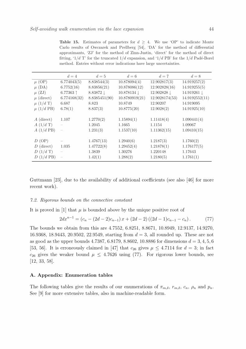
Self-avoiding walk enumeration via the lace expansion 44
Table 15. Estimates of parameters for d ≥ 4. We use ‘OP’ to indicate MonteCarlo results of Owczarek and Prellberg [54], ‘DA’ for the method of differentialapproximants, ‘ZJ’ for the method of Zinn-Justin, ‘direct’ for the method of directfitting, ‘1/d T’ for the truncated 1/d expansion, and ‘1/d PB’ for the 1/d Pade-Borelmethod. Entries without error indications have large uncertainties.
d = 4 d = 5 d = 6 d = 7 d = 8µ (OP) 6.774043(5) 8.838544(3) 10.878094(4) 12.902817(3) 14.919257(2)µ (DA) 6.7752(16) 8.83856(21) 10.878086(12) 12.902828(16) 14.919255(5)µ (ZJ) 6.77363 ↑ 8.83872 ↓ 10.878134 ↓ 12.902828 ↓ 14.919261 ↓µ (direct) 6.774168(32) 8.8385451(90) 10.8780919(21) 12.9028174(53) 14.9192552(11)µ (1/d T) 6.687 8.823 10.8749 12.90207 14.919095µ (1/d PB) 6.78(1) 8.837(3) 10.8775(20) 12.9028(2) 14.91925(10)
A (direct) 1.107 1.2770(2) 1.15894(1) 1.11418(4) 1.090441(4)A (1/d T) – 1.2045 1.1665 1.1154 1.09067A (1/d PB) – 1.231(3) 1.1537(10) 1.11362(15) 1.09410(15)
D (OP) – 1.4767(13) 1.2940(6) 1.2187(3) 1.1760(2)D (direct) 1.035 1.47722(8) 1.29452(4) 1.21878(1) 1.176177(5)D (1/d T) – 1.3839 1.30276 1.220148 1.17643D (1/d PB) – 1.42(1) 1.288(2) 1.2180(5) 1.1761(1)
Guttmann [23], due to the availability of additional coefficients (see also [46] for more
recent work).
7.2. Rigorous bounds on the connective constant
It is proved in [1] that µ is bounded above by the unique positive root of
2dxn−1 = (cn − (2d− 2)cn−1) x + (2d− 2) ((2d− 1)cn−1 − cn) . (77)
The bounds we obtain from this are 4.7552, 6.8251, 8.8671, 10.8949, 12.9137, 14.9270,
16.9368, 18.9443, 20.9502, 22.9549, starting from d = 3, all rounded up. These are not
as good as the upper bounds 4.7387, 6.8179, 8.8602, 10.8886 for dimensions d = 3, 4, 5, 6
[53, 56]. It is erroneously claimed in [47] that c26 gives µ ≤ 4.7114 for d = 3; in fact
c26 gives the weaker bound µ ≤ 4.7626 using (77). For rigorous lower bounds, see
[12, 33, 58].
A. Appendix: Enumeration tables
The following tables give the results of our enumerations of πm,δ, rm,δ, cn, ρn and pn.
See [9] for more extensive tables, also in machine-readable form.
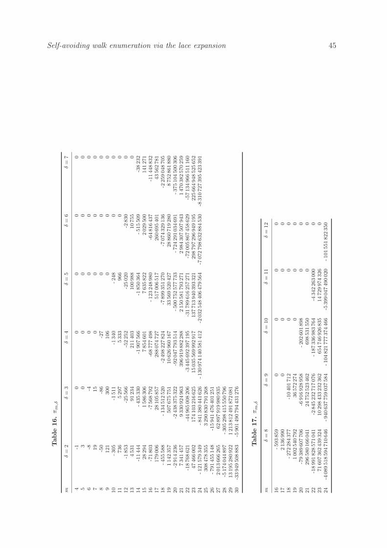
Self-avoiding walk enumeration via the lace expansion 45Tab
le16
.π
m,δ
mδ
=2
δ=
3δ
=4
δ=
5δ
=6
δ=
7
4-1
00
00
05
30
00
00
6-8
-40
00
07
19
15
00
00
8-5
0-8
6-2
70
00
9121
300
106
00
010
-305
-1511
-1340
-248
00
11
736
5297
5333
966
00
12
-1853
-25
566
-52
252
-25
020
-2830
013
4531
91
234
211
403
100
988
10
755
014
-11
444
-435
330
-1907
566
-1850
364
-515
509
-38
232
15
28
294
1586
306
7854
601
7635
822
2029
500
141
271
16
-71
803
-7568
792
-68
777
498
-123
248
980
-64
816
437
-11
448
832
17
179
006
28
105
857
288
074
727
517
006
517
260
695
401
43
562
781
18
-455
588
-134
512
520
-2498
227
824
-7899
351
270
-7074
329
136
-2259
048
705
19
1142
357
507
675
751
10
626
960
167
33
569
520
427
28
860
719
280
8752
861
880
20
-2914
236
-2438
375
322
-92
047
793
514
-500
752
577
733
-724
291
034
691
-375
104
500
306
21
7341
457
9330
924
963
396
919
882
288
2150
581
793
271
2984
307
507
943
1470
382
570
259
22
-18
768
621
-44
965
008
206
-3445
692
397
195
-31
789
616
257
271
-72
005
867
458
629
-57
134
966
511
160
23
47
466
002
174
103
216
625
15
035
569
992
917
137
713
940
393
321
298
797
296
949
195
225
664
948
525
652
24
-121
579
349
-841
380
441
626
-130
974
140
581
412
-2032
548
406
479
564
-7072
798
632
884
530
-8310
727
395
423
391
25
308
478
355
3290
830
791
268
26
-791
455
148
-15
941
476
401
251
27
2013
666
265
62
897
919
980
935
28
-5174
044
897
-305
298
415
550
796
29
13
195
280
922
1213
812
491
872
081
30
-33
949
508
883
-5901
490
794
431
276
Tab
le17
.π
m,δ
mδ
=8
δ=
9δ
=10
δ=
11
δ=
12
16
-593
859
00
00
17
2136
990
00
00
18
-272
284
377
-10
401
712
00
019
1002
540
792
36
572
274
00
020
-79
389
607
706
-6916
928
958
-202
601
898
00
21
296
580
166
041
24
752
523
462
698
531
550
00
22
-18
991
828
571
041
-2845
232
717
076
-187
336
983
764
-4342
263
000
023
71
607
362
439
324
10
298
433
232
362
654
746
926
835
14
729
974
326
024
-4089
518
594
710
646
-940
637
759
037
584
-104
821
777
374
466
-5399
047
490
020
-101
551
822
350
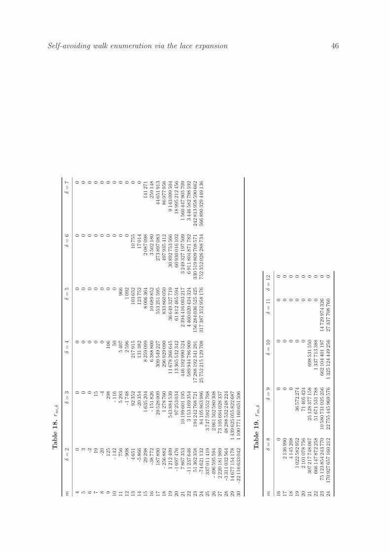
Self-avoiding walk enumeration via the lace expansion 46Tab
le18
.r m
,δ
mδ
=2
δ=
3δ
=4
δ=
5δ
=6
δ=
7
40
00
00
05
30
00
00
6-2
00
00
07
19
15
00
00
8-2
0-4
00
00
9125
298
106
00
010
-142
-116
50
00
011
756
5293
5407
966
00
12
-908
-1748
2596
1092
00
13
4651
92
352
217
915
103
652
10
755
014
-5866
-20
354
131
382
123
752
17
014
015
29
298
1635
204
8259
099
8006
364
2087
098
141
271
16
-38
772
-151
826
6388
800
10
689
852
3502
180
259
148
17
187
890
29
528
009
309
549
227
553
251
595
273
897
083
44
651
913
18
-256
882
1278
760
296
929
090
833
860
050
497
935
412
86
977
956
19
1212
409
543
884
539
11
678
266
645
36
649
327
719
30
892
753
566
9143
099
504
20
-1697
476
97
253
034
13
365
532
342
61
812
465
594
60
930
016
102
18
995
212
456
21
7867
353
10
199
601
195
446
192
990
524
2394
416
093
217
3249
327
197
509
1560
447
905
709
22
-11
237
646
3153
169
354
589
944
786
900
4460
020
424
324
6911
804
871
782
3446
582
798
592
23
51
362
358
194
242
768
721
17
288
192
341
291
156
284
036
525
425
330
519
809
708
571
242
813
958
590
662
24
-74
621
132
84
105
863
986
25
752
215
129
708
317
387
352
958
176
752
352
026
288
734
566
890
329
449
136
25
337
011
419
3747
592
552
768
26
-496
595
594
2061
502
580
308
27
2220
181
989
73
105
694
028
337
28
-3311
032
564
48
288
532
248
224
29
14
677
154
178
1439
625
055
822
687
30
-22
116
633
042
1100
771
160
651
506
Tab
le19
.r m
,δ
mδ
=8
δ=
9δ
=10
δ=
11
δ=
12
16
00
00
017
2136
990
00
00
18
4145
208
00
00
19
1022
582
952
36
572
274
00
020
2101
078
756
71
405
424
00
021
307
217
748
067
25
128
377
158
698
531
550
00
22
666
147
872
258
51
671
531
788
1337
713
388
00
23
75
123
854
243
770
10
580
731
025
256
662
104
401
197
14
729
974
326
024
170
927
657
160
212
22
755
445
969
576
1325
124
449
256
27
337
708
760
0
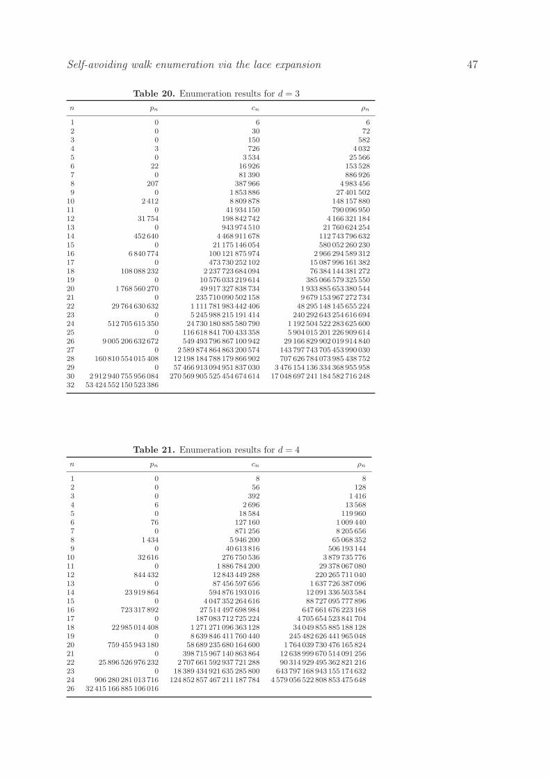
Self-avoiding walk enumeration via the lace expansion 47
Table 20. Enumeration results for d = 3n pn cn ρn
1 0 6 62 0 30 723 0 150 5824 3 726 4 0325 0 3 534 25 5666 22 16 926 153 5287 0 81 390 886 9268 207 387 966 4 983 4569 0 1 853 886 27 401 502
10 2 412 8 809 878 148 157 88011 0 41 934 150 790 096 95012 31 754 198 842 742 4 166 321 18413 0 943 974 510 21 760 624 25414 452 640 4 468 911 678 112 743 796 63215 0 21 175 146 054 580 052 260 23016 6 840 774 100 121 875 974 2 966 294 589 31217 0 473 730 252 102 15 087 996 161 38218 108 088 232 2 237 723 684 094 76 384 144 381 27219 0 10 576 033 219 614 385 066 579 325 55020 1 768 560 270 49 917 327 838 734 1 933 885 653 380 54421 0 235 710 090 502 158 9 679 153 967 272 73422 29 764 630 632 1 111 781 983 442 406 48 295 148 145 655 22423 0 5 245 988 215 191 414 240 292 643 254 616 69424 512 705 615 350 24 730 180 885 580 790 1 192 504 522 283 625 60025 0 116 618 841 700 433 358 5 904 015 201 226 909 61426 9 005 206 632 672 549 493 796 867 100 942 29 166 829 902 019 914 84027 0 2 589 874 864 863 200 574 143 797 743 705 453 990 03028 160 810 554 015 408 12 198 184 788 179 866 902 707 626 784 073 985 438 75229 0 57 466 913 094 951 837 030 3 476 154 136 334 368 955 95830 2 912 940 755 956 084 270 569 905 525 454 674 614 17 048 697 241 184 582 716 24832 53 424 552 150 523 386
Table 21. Enumeration results for d = 4n pn cn ρn
1 0 8 82 0 56 1283 0 392 1 4164 6 2 696 13 5685 0 18 584 119 9606 76 127 160 1 009 4407 0 871 256 8 205 6568 1 434 5 946 200 65 068 3529 0 40 613 816 506 193 144
10 32 616 276 750 536 3 879 735 77611 0 1 886 784 200 29 378 067 08012 844 432 12 843 449 288 220 265 711 04013 0 87 456 597 656 1 637 726 387 09614 23 919 864 594 876 193 016 12 091 336 503 58415 0 4 047 352 264 616 88 727 095 777 89616 723 317 892 27 514 497 698 984 647 661 676 223 16817 0 187 083 712 725 224 4 705 654 523 841 70418 22 985 014 408 1 271 271 096 363 128 34 049 855 885 188 12819 0 8 639 846 411 760 440 245 482 626 441 965 04820 759 455 943 180 58 689 235 680 164 600 1 764 039 730 476 165 82421 0 398 715 967 140 863 864 12 638 999 670 514 091 25622 25 896 526 976 232 2 707 661 592 937 721 288 90 314 929 495 362 821 21623 0 18 389 434 921 635 285 800 643 797 168 943 155 174 63224 906 280 281 013 716 124 852 857 467 211 187 784 4 579 056 522 808 853 475 64826 32 415 166 885 106 016
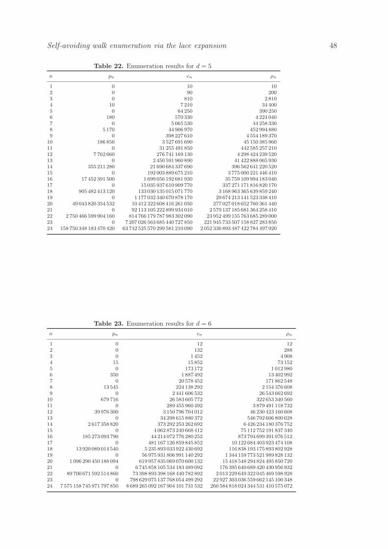
Self-avoiding walk enumeration via the lace expansion 48
Table 22. Enumeration results for d = 5n pn cn ρn
1 0 10 102 0 90 2003 0 810 2 8104 10 7 210 34 4005 0 64 250 390 2506 180 570 330 4 224 0407 0 5 065 530 44 258 3308 5 170 44 906 970 452 994 8809 0 398 227 610 4 554 189 370
10 186 856 3 527 691 690 45 150 385 96011 0 31 255 491 850 442 585 257 21012 7 762 660 276 741 169 130 4 298 424 239 52013 0 2 450 591 960 890 41 422 888 065 93014 355 211 280 21 690 684 337 690 396 562 641 220 52015 0 192 003 889 675 210 3 775 000 221 446 41016 17 452 391 500 1 699 056 192 681 930 35 759 109 994 183 04017 0 15 035 937 610 909 770 337 271 171 816 820 17018 905 482 413 120 133 030 135 015 071 770 3 168 963 365 639 859 24019 0 1 177 032 340 670 878 170 29 674 213 141 523 338 41020 49 043 820 354 532 10 412 322 608 416 261 050 277 027 018 652 760 361 44021 0 92 113 105 222 899 934 010 2 579 137 185 681 364 258 41022 2 750 466 599 904 160 814 766 179 787 983 302 090 23 952 499 155 763 685 289 00023 0 7 207 026 563 685 440 727 850 221 945 733 507 158 827 283 85024 158 750 348 183 470 420 63 742 525 570 299 581 210 090 2 052 336 893 487 422 784 497 920
Table 23. Enumeration results for d = 6n pn cn ρn
1 0 12 122 0 132 2883 0 1 452 4 9084 15 15 852 73 1525 0 173 172 1 012 9806 350 1 887 492 13 402 9927 0 20 578 452 171 862 5488 13 545 224 138 292 2 154 376 6089 0 2 441 606 532 26 543 662 692
10 679 716 26 583 605 772 322 653 340 56011 0 289 455 960 492 3 879 491 118 73212 39 976 300 3 150 796 704 012 46 230 423 160 60813 0 34 298 615 880 372 546 792 606 800 62814 2 617 358 820 373 292 253 262 692 6 426 234 180 376 75215 0 4 062 873 240 668 412 75 112 752 191 837 34016 185 273 093 790 44 214 072 776 280 252 873 794 699 391 076 51217 0 481 167 126 859 845 852 10 122 684 403 923 474 10818 13 920 089 014 540 5 235 893 033 922 430 692 116 838 193 175 893 802 92819 0 56 975 931 806 991 140 292 1 344 159 773 521 989 828 13220 1 096 290 450 188 094 619 957 835 069 070 600 132 15 418 548 294 824 495 850 72021 0 6 745 858 105 534 183 489 092 176 395 640 689 420 430 956 93222 89 700 671 592 514 860 73 398 893 398 168 440 782 892 2 013 229 649 322 045 469 598 92823 0 798 629 075 137 768 054 499 292 22 927 303 036 559 662 145 100 34824 7 575 158 745 971 797 850 8 689 265 092 167 904 101 731 532 260 584 818 024 344 531 410 575 072
Self-avoiding walk enumeration via the lace expansion 49
Acknowledgments
NC acknowledges support by the Australian Research Council and the Centre of
Excellence for Mathematics and Statistics of Complex Systems. RL acknowledges
the support of Postgraduate Scholarships from NSERC of Canada. The work of GS
was supported in part by NSERC. We benefited from the Pacific Institute for the
Mathematical Sciences 2005 Summer School in Probability, during which we had the
opportunity to work together. We thank Tony Guttmann and Andrew Rechnitzer for
helpful discussions. All numerical calculations were performed using the computational
resources of the Victorian Partnership for Advanced Computing (VPAC).
References
[1] R. Ahlberg and S. Janson. Upper bounds for the connective constant. Unpublished manuscript,(1980).
[2] P. Belohorec. Renormalization group calculation of the universal critical exponents of a polymermolecule. PhD thesis, University of Guelph, (1997).
[3] D.C. Brydges and J.Z. Imbrie. End-to-end distance from the Green’s function for a hierarchicalself-avoiding walk in four dimensions. Commun. Math. Phys., 239:523–547, (2003).
[4] D.C. Brydges and T. Spencer. Self-avoiding walk in 5 or more dimensions. Commun. Math. Phys.,97:125–148, (1985).
[5] M. Campostrini, A. Pelissetto, P. Rossi, and E. Vicari. 25th-order high-temperature expansionresults for three-dimensional Ising-like systems on the simple-cubic lattice. Phys. Rev. E,65:066127, (2002).
[6] S. Caracciolo, M.S. Causo, and A. Pelissetto. High-precision determination of the critical exponentγ for self-avoiding walks. Phys. Rev. E, 57:1215–1218, (1998).
[7] S. Caracciolo, A.J. Guttmann, I. Jensen, A. Pelissetto, A.N. Rogers, and A.D. Sokal. Correctionto scaling exponents for two-dimensional self-avoiding walks. J. Statist. Phys., 120:1037–1100,(2005).
[8] M. Chen and K.Y. Lin. Amplitude ratios for self-avoiding walks on hypercubic lattices in 4 to 6dimensions. Chinese J. Phys., 41:52–58, (2003).
[9] N. Clisby, R. Liang, and G. Slade. Self-avoiding walk enumeration via the lace expansion: tables.Unpublished, (2007). http://www.math.ubc.ca/∼slade/lacecounts has enumeration data inmachine-readable form.
[10] N. Clisby and G. Slade. In preparation.[11] A.R. Conway, I.G. Enting, and A.J. Guttmann. Algebraic techniques for enumerating self-avoiding
walks on the square lattice. J. Phys. A: Math. Gen., 26:1519–1534, (1993).[12] A.R. Conway and A.J. Guttmann. Lower bound on the connective constant for square lattice
self-avoiding walks. J. Phys. A: Math. Gen., 26:3719–3724, (1993).[13] B. Duplantier. Polymer chains in four dimensions. Nuclear Physics B, 275 [FS17]:319–355, (1986).[14] M.E. Fisher and D.S. Gaunt. Ising model and self-avoiding walks on hypercubical lattices and
“high-density” expansions. Phys. Rev., 133:A224–A239, (1964).[15] M.E. Fisher and R.R.P. Singh. Critical points, large-dimensionality expansions, and the Ising spin
glass. In G.R. Grimmett and D.J.A. Welsh, editors, Disorder in Physical Systems. ClarendonPress, Oxford, (1990).
[16] M.E. Fisher and M.F. Sykes. Excluded-volume problem and the Ising model of ferromagnetism.Phys. Rev., 114:45–58, (1959).
[17] D.S. Gaunt. 1/d expansions for critical amplitudes. J. Phys. A: Math. Gen., 19:L149–L153,(1986).
Self-avoiding walk enumeration via the lace expansion 50
[18] D.S. Gaunt and A.J. Guttmann. Asymptotic analysis of coefficients. In C. Domb and M.S. Green,editors, Phase Transitions and Critical Phenomena, Volume 3, pages 181–243. Academic Press,New York, (1974).
[19] P.R. Gerber and M.E. Fisher. Critical temperatures of classical n-vector models on hypercubiclattices. Phys. Rev. B, 10:4697–4703, (1974).
[20] P. Grassberger, R. Hegger, and L. Schafer. Self-avoiding walks in four dimensions: logarithmiccorrections. J. Phys. A: Math. Gen., 27:7265–7282, (1994).
[21] R. Guida and J. Zinn-Justin. Critical exponents of the N -vector model. J. Phys. A: Math. Gen.,31:8103–8121, (1998).
[22] A. J. Guttmann and S. G. Whittington. Two-dimensional lattice embeddings of connected graphsof cyclomatic index two. J. Phys. A: Math. Gen., 11:721–729, (1978).
[23] A.J. Guttmann. On the zero-field susceptibility in the d = 4, n = 0 limit: analysing for confluentlogarithmic singularities. J. Phys. A: Math. Gen., 11:L103–L106, (1978).
[24] A.J. Guttmann. Correction to scaling exponents and critical properties of the n-vector model withdimensionality > 4. J. Phys. A: Math. Gen., 14:233–239, (1981).
[25] A.J. Guttmann. On the critical behaviour of self-avoiding walks. J. Phys. A: Math. Gen., 20:1839–1854, (1987).
[26] A.J. Guttmann. Asymptotic analysis of power-series expansions. In C. Domb and J.L. Lebowitz,editors, Phase Transitions and Critical Phenomena, Volume 13, pages 1–234. Academic Press,New York, (1989).
[27] A.J. Guttmann. On the critical behaviour of self-avoiding walks: II. J. Phys. A: Math. Gen.,22:2807–2813, (1989).
[28] A.J. Guttmann and J. Wang. The extension of self-avoiding random walk series in two dimensions.J. Phys. A: Math. Gen., 24:3107–3109, (1991).
[29] J.M. Hammersley and K.W. Morton. Poor man’s Monte Carlo. J. Roy. Stat. Soc. B, 16:23–38,(1954).
[30] T. Hara and G. Slade. The lace expansion for self-avoiding walk in five or more dimensions.Reviews in Math. Phys., 4:235–327, (1992).
[31] T. Hara and G. Slade. Self-avoiding walk in five or more dimensions. I. The critical behaviour.Commun. Math. Phys., 147:101–136, (1992).
[32] T. Hara and G. Slade. The self-avoiding-walk and percolation critical points in high dimensions.Combin. Probab. Comput., 4:197–215, (1995).
[33] T. Hara, G. Slade, and A.D. Sokal. New lower bounds on the self-avoiding-walk connectiveconstant. J. Statist. Phys., 72:479–517, (1993). Erratum: J. Statist. Phys., 78:1187–1188,(1995).
[34] R. van der Hofstad and G. Slade. The lace expansion on a tree with application to networks ofself-avoiding walks. Adv. Appl. Math., 30:471–528, (2003).
[35] R. van der Hofstad and G. Slade. Expansion in n−1 for percolation critical values on the n-cubeand Zn: the first three terms. Combin. Probab. Comput., 15:695–713, (2006).
[36] H.-P. Hsu and P. Grassberger. Polymers confined between two parallel plane walls. J. Chem.Phys., 120:2034–2041, (2004).
[37] H.-P. Hsu, W. Nadler, and P. Grassberger. Scaling of star polymers with 1–80 arms.Macromolecules, 37:4658–4663, (2004).
[38] B.D. Hughes. Random Walks and Random Environments, volume 1: Random Walks. OxfordUniversity Press, Oxford, (1995).
[39] D.L. Hunter and G.A. Baker Jr. Methods of series analysis. III. Integral approximant methods.Phys. Rev., B19:3808–3821, (1979).
[40] I. Jensen. A parallel algorithm for the enumeration of self-avoiding polygons on the square lattice.J. Phys. A: Math. Gen., 36:5731–5745, (2003).
[41] I. Jensen. Enumeration of self-avoiding walks on the square lattice. J. Phys. A: Math. Gen.,37:5503–5524, (2004).
Self-avoiding walk enumeration via the lace expansion 51
[42] H. Kesten. On the number of self-avoiding walks. II. J. Math. Phys., 5:1128–1137, (1964).[43] H. Kleinert and V. Schulte-Frohlinde. Critical Properties of φ4-Theories. World Scientific,
Singapore, (2001).[44] D.E. Knuth. The Art of Computer Programming, Volume 3. Addison Wesley, Reading, (1973).[45] B. Li, N. Madras, and A.D. Sokal. Critical exponents, hyperscaling, and universal amplitude ratios
for two- and three-dimensional self-avoiding walks. J. Statist. Phys., 80:661–754, (1995).[46] B. MacDonald, D.L. Hunter, K. Kelly, and N. Jan. Self-avoiding walks in two to five dimensions:
exact enumerations and series study. J. Phys. A: Math. Gen., 25:1429–1440, (1992).[47] B. MacDonald, S. Joseph, D.L. Hunter, L.L. Moseley, N. Jan, and A.J. Guttmann. Self-avoiding
walks on the simple cubic lattice. J. Phys. A: Math. Gen., 33:5973–5983, (2000).[48] N. Madras and G. Slade. The Self-Avoiding Walk. Birkhauser, Boston, (1993).[49] N. Madras and A.D. Sokal. The pivot algorithm: A highly efficient Monte Carlo method for the
self-avoiding walk. J. Statist. Phys., 50:109–186, (1988).[50] B. McKay, W. Myrvold, and J. Nadon. Fast backtracking principles applied to find new cages.
In 9th Annual ACM-SIAM Symposium on Discrete Algorithms, pages 188–191, (1998).[51] A.M. Nemirovsky, K.F. Freed, T. Ishinabe, and J.F. Douglas. End-to-end distance of a single self-
interacting self-avoiding polymer chain: d−1 expansion. Phys. Lett. A, 162:469–474, (1992).[52] A.M. Nemirovsky, K.F. Freed, T. Ishinabe, and J.F. Douglas. Marriage of exact enumeration
and 1/d expansion methods: Lattice model of dilute polymers. J. Statist. Phys., 67:1083–1108,(1992).
[53] J. Noonan. New upper bounds on the connective constants of self-avoiding walks. J. Statist.Phys., 91:871–888, (1998).
[54] A.L. Owczarek and T. Prellberg. Scaling of self-avoiding walks in high dimensions. J. Phys. A:Math. Gen., 34:5773–5780, (2001).
[55] A. Pelissetto and E. Vicari. Critical phenomena and renormalization-group theory. Phys. Reports,368:549–727, (2002).
[56] A. Ponitz and P. Tittmann. Improved upper bounds for self-avoiding walks in Zd. Electron. J.Combin., 7:Paper R21, (2000).
[57] T. Prellberg. Scaling of self-avoiding walks and self-avoiding trails in three dimensions. J. Phys.A: Math. Gen., 34:L599–L602, (2001).
[58] G. Slade. Bounds on the self-avoiding-walk connective constant. Journal of Fourier Analysisand Applications, Special Issue: Proceedings of the Conference in Honor of Jean-Pierre Kahane(Orsay, June 28 – July 3 1993):525–533, (1995).
[59] G. Slade. The Lace Expansion and its Applications. Springer, Berlin, (2006). Lecture Notes inMathematics Vol. 1879. Ecole d’Ete de Probabilites de Saint–Flour XXXIV–2004.
[60] E. Swierczak. Numerical problems in statistical mechanics. PhD thesis, University of Melbourne,(1995).
[61] G. Torrie and S.G. Whittington. Exact enumeration of neighbour-avoiding walks on the tetrahedraland body-centred cubic lattices. J. Phys. A: Math. Gen., 8:1178–1184, (1975).
[62] J. Zinn-Justin. Analysis of Ising-model critical exponents from high-temperature series expansion.J. Phys. (France), 40:969–975, (1979).
[63] J. Zinn-Justin. Analysis of high-temperature series of the spin-s Ising model on the body-centredcubic lattice. J. Phys. (France), 42:783–792, (1981).