Biol. Cybern. 43, 59-69 (1982) Biological Cybernetics �9 Springer-Verlag 1982

Self-Organized Formation of Topologically Correct Feature Maps

Teuvo Kohonen Department of Technical Physics, Helsinki University of Technology, Espoo, Finland

Abstract. This work contains a theoretical study and computer simulations of a new self-organizing process. The principal discovery is that in a simple network of adaptive physical elements which receives signals from a primary event space, the signal representations are automatically mapped onto a set of output responses in such a way that the responses acquire the same topological order as that of the primary events. In other words, a principle has been discovered which facilitates the automatic formation of topologically correct maps of features of observable events. The basic self-organizing system is a one- or two- dimensional array of processing units resembling a network of threshold-logic units, and characterized by short-range lateral feedback between neighbouring units. Several types of computer simulations are used to demonstrate the ordering process as well as the conditions under which it fails.

1. ln~oducfion

The present work has evolved from a recent discovery by the author (Kohonen, 1981), i.e. that topologically correct maps of structured distributions of signals can be formed in, say, a one- or two-dimensional array of processing units which did not have this structure initially. This principle is a generalization of the for- mation of direct topographic projections between two laminar structures known as retinotectal mapping (Willshaw and Malsburg, 1976, 1979; Malsburg and Willshaw, 1977; Amari, 1980). It will be introduced here in a general form in which signals of any modality may be used. There are no restrictions on the auto- matic formation of maps of completely abstract or conceptual items provided their signal representations or feature values are expressible in a metric or to- pological space which allows their ordering. In other

words, we shall not restrict ourselves to topographical maps but consider maps of patterns relating to an arbitrary feature or attribute space, and at any level of abstraction.

The processing units by which these mappings are implemented can be identified with concrete physical adaptive components of a type similar to the Perceptrons (Rosenblatt, 1961). There is a characteris- tic feature in these new models, namely, a local feed- back which makes map formation possible. The main objective of this work has been to demonstrate that external signal activity alone, assuming a proper struc- tural and functional description of system behavior, is sufficient for enforcing mappings of the above kind into the system.

The present work is related to an idealized neural structure. However, the intention is by no means to assert that self-organization is mainly of neural origin; on the contrary, there are good reasons to assume that the basic state of readiness is often determined geneti- cally. This does not exclude the possibility, however, that self-organization may significantly be affected and sometimes even completely determined by sensory experiences. On the other hand, the logic underlying this model is readily generalizable to mechanisms other than neural.

There are indeed many kinds of maps or images of sensory experiences in the brain; the most familiar ones are the retinotopic, somatotopic, and tonotopic projections in the primary sensory areas, as well as the somatotopic order of cells in the motor cortex. There is some evidence (Lynch et al., 1978) that topographic maps of the exterior environment are formed in the hippocampus. These observations suggest that the brains of different species would also more generally be able to produce maps of occurrences that are only indirectly related to the sensory inputs ; notice that the signals received by the sensory areas have also been transformed by sensory organs, ganglia, and relay

0340-1200/82/0043/0059/$02.20

60

nuclei. If the ability to form maps were ubiquitous in the brain, then one could easily explain its power to operate on semantic items: some areas of the brain could simply create and order specialized cells or cell groups in conformity with high-level features and their combinations.

The possibility of constructing spatial maps for attributes and features in fact revives the old question of how symbolic representations for concepts could.be formed automatically; most of the models of automatic problem solving and representation of knowledge have simply skipped this question.

2. Preliminary Simulations

In order to elucidate the self-organizing processes discussed in this paper, their operation is first demon- strated by means of ultimately simplified system mo- dels. The essential constituents of these systems are: 1. An array of processing units which receive coherent inputs from an event space and form simple discri- minant functions of their input signals. 2. A mecha- nism which compares the discriminant functions and selects the unit with the greatest function value. 3. Some kind of local interaction which simultaneously activates the selected unit and its nearest neighbours. 4. An adaptive process which makes the parameters of the activated units increase their discriminant function values relating to the present input.

2.1. Definition of Ordered Mappings

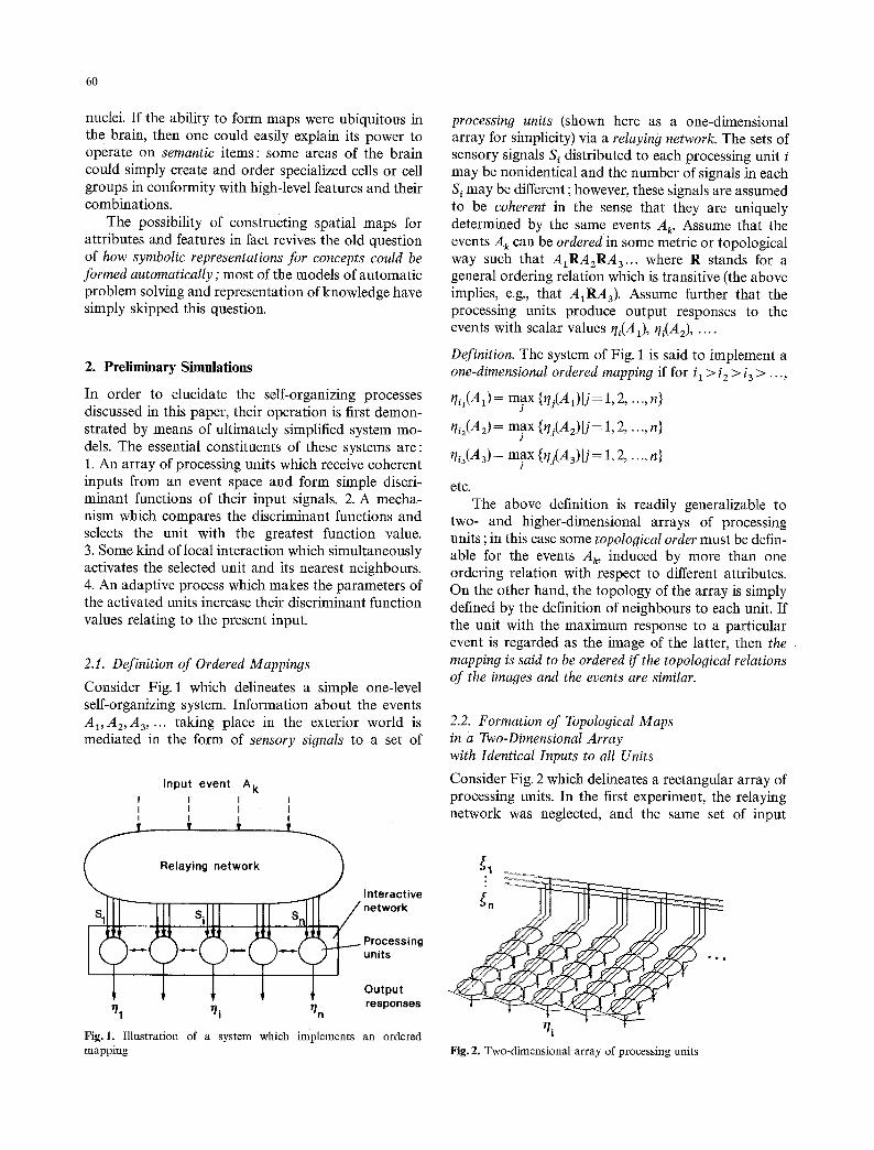
Consider Fig. 1 which delineates a simple one-level self-organizing system. Information about the events A1,A2,A3,... taking place in the exterior world is mediated in the form of sensory signals to a set of

I n p u t e v e n t A k I I I I I I I I I I I I

Relaying network J Interactive

SI[II- [ I Sill[ 111 ~ / n e t w o r k

~.._. ~._. ~ ~.,,_. ~....~ ~... Processing "J [ units Output T/1 r/i r/n responses

Fig. 1. Illustration of a system which implements an ordered mapping

processing units (shown here as a one-dimensional array for simplicity) via a relaying network. The sets of sensory signals S i distributed to each processing unit i may be nonidentical and the number of signals in each Si may be different; however, these signals are assumed to be coherent in the sense that they are uniquely determined by the same events A k. Assume that the events A k can be ordered in some metric or topological way such that A1RAzRA3... where R stands for a general ordering relation which is transitive (the above implies, e.g., that A1RA3). Assume further that the processing units produce output responses to the events with scalar values th(A0, t/i(A2) . . . . .

Definition. The system of Fig. 1 is said to implement a one-dimensional ordered mapping if for i t > i z > i 3 > . . . ,

t/q(A1) : max {~/j(A a)Ij = 1, 2,..., n} J

qi2(A2) = max {tlj(Az)[j = 1, 2,..., n} J

qi3(A3) = max {t/j(A3)lJ = 1, 2,..., n} J

etc. The above definition is readily generalizable to

two- and higher-dimensional arrays of processing units; in this case some topological order must be defin- able for the events Ak, induced by more than one ordering relation with respect to different attributes. On the other hand, the topology of the array is simply defined by the definition of neighbours to each unit. If the unit with the maximum response to a particular event is regarded as the image of the latter, then the mapping is said to be ordered if the topological relations of the images and the events are similar.

2.2. Formation of Topological Maps in a Two-Dimensional Array with Identical Inputs to all Units

Consider Fig. 2 which delineates a rectangular array of processing units. In the first experiment, the relaying network was neglected, and the same set of input

qi Fig, 2. Two-dimensional array of processing units

61

~2

,-" ~ :.._".; ... -: .. ".:";. :... . .~ '-,.

, . " - ' " , " . : . : ' : ' ; : . " " ' . , ' : " " ' . ' ~ . " " ~i [.-,-. . - - ' ' ,,:= :. :..'. ," -:1 I !~. " . - : ' . . ' . ' " "::''. L : . ; . ' : : . _= - . . ' 4 I

i F,::. ,:-.::..:_ " }1' v..~.: .': 4 ." .'-" '.,:;": ","."',i.~):i): t ,/ ',, -,-..:....c'.:,.:..v. . I . ? " : . . :,:; ,,"

' \ " "" , " " ' -"- ":" " : 0 , " " : ~"" ' ' ": ' r �9 . ~.x.." ' , ' : " ~, " , ' - ; r ' " ; - ' . . _ . _ ~ . "

( a )

( i l , i 2 ) i2--.-~ 'W . ~ " , " ~ ( ~ r o '

i l 1 2 " d 4 5 o ' 7 8 ;:--.~" '>-.~ >-< >--:: :----< ?=-'-(-. >--< ..:.--< 1 / . . . . . . ' . (Z 1":,[2 ~'(2 z',(2 4"{a 5Xz ;~,i z zXa s)

I 2 . . . . . . . . "\ ::---<~< >-< ...'>--I, [::-~..'.--~. ~< >-=; / 3 . ". 3 1',(3 zY., 3X3 4 ~ 5 t,3 6)<3 ;),.~ ,., /

. . . . . . . . '/ " >

, " ( - " ,": " 5r . . . . .

,% 6 . . . . . . . . / >.--:C'.~-:._ , , , , . " : '~)L<} ' : '~>- '<, ;>~<., , , . , . ,~.

q . . . . . . . . ," .>-< >-< >-< >-<,>-<,,>~..'_~5-, ~-~ 8:,. . . . . . . / (7 ~',(7..',~z.-.'b,4) ;t,.-'~Xz?,(,-'~) �9 .. .,..' ~ - ~ . . . . g " .~, .~" ~,._ _, ' %. ./

'" -~" 4 -~ y:~?,o : . . . . . . . . . . . . " ~,i~8-, ~84(~5 ~ . ~ X a , s) �9 ,:~..,',,__',".,.:_:., ..,__..,.,.__.. ',:J ,~.. ',.j

( b ) ( c )

Fig. 3. a Distribution of training vectors (front view of the surface of a unit sphere in Ra). The distribution had edges, each of which contained as many vectors as the inside, b Test vectors which are mapped into the outputs of the processing unit array, e Images of the test vectors at the outputs

signals {41, ~ 2 ' ' ' " ~n} was connected to all units. In accordance with notations used in mathematical sys- tem theory, this set of signals is expressed as a column vector x=[~l ,~2, . . . ,~ ,]TeR" where T denotes the transpose. Unit i shall have input weights or parame- ters #~l,#iz,-..,#~, which are expressible as another

�9 1 T E R n column v e c t o r mi=Fflil,#i2,...,i.~in d . The unit shall form the discriminant function

~= ~ ~u~j=mrx. (1) j = l

A discrimination mechanism (Sect. 3) shall further operate by which the maximum of the q~ is singled out:

ilk = max {th}. (2)

For unit k and all the eight of its nearest neighbours (except at the edges of the array where the number of neighbours was different) the following adaptive pro- cess is then assumed to be active"

mi(t+ 1)= mi(t)+c~x(t) I I mi(t) + c~x(t) llE' (3)

where the variables have been labelled by a discrete- time index t (an integer), ~ is a "gain parameter" in adaptation, and the denominator is the Euclidean norm of the numerator. Equation (3) otherwise re- sembles the well-known teaching rule of the Perceptron, except that the direction of the corrections is always the same as that of x (no decision process or supervision is involved), and the weight vectors are normalized. Normalization improves selectivity in dis- crimination, and it is also beneficial in maintaining the "memory resources" at a certain level. Notice that the process of Eq. (3) does not change the length of m i but only rotates m i towards x. Nonetheless it is not always

necessary that the norm be Euclidean as in Eq. (3) (Sect. 3.3).

Simulation 1. A sequence of training vectors {x(t)} was derived from the structured distribution shown in Fig. 3a. Without much loss of generality, the lengths of the x(t) were normalized to unity whereby their distri- bution lies on the surface of the unit sphere in R 3. The "training vectors" were picked up noncyclically, in a completely random fashion from this distribution. The initial values for the parameters #u were also defined as random numbers. The gain parameter e was made a function of the iteration step, e.g., proportional to lit. (A decreasing sequence was necessary for stabilization, and this choice complies with that frequently used in mathematical models of learning systems.)

To test the final state of the system after many iterations, a set of test vectors from the distribution of Fig. 3 a, as shown in Fig. 3 b, was defined. The images of these vectors (i.e. those units which gave the largest responses to particular input vectors) are shown in Fig. 3 c. It may be clearly discernible that an ordered mapping has been formed in the process. The map has also formatted itself along the sides of the array.

What actually caused the self-ordering ? Some fun- damental properties of this process can be determined by means of the following argumentation. The cor- rective process of Eq. (3) increases the parallelism of the activated (neighbouring) vectors. Thus the differen- tial order all over the array will be increased on the average. However, differential ordering steps of the above kind cannot take place independently of each other. As all units in the array have neighbours which they affect during adaptation, changes in individual units cannot be compatible unless they result in a global order. The boundary effects in the array delimit the

62

100 j

" / J

~- 1 -. 500 f . . . . . . ~--- . . .

R, " -J/" 'x % ./

2000 j--------"-- . .

,f'/

( "~k.

",% '~"'--~..__ __...~.. l'~'

10000 -.----------~ .... f t ~*"~"x /' ''/ r - ' g ' 2 - ~ ~ \',.,..,

Fig. 4. Distribution of the weight vectors rn~(t) at different times. The number of training steps is shown above the distribution. Interaction between nearest neighbours only

format of the map in a manner somewhat similar to the way boundary conditions determine the solution of a differential equation.

Simulation 2. A clear conception of the ordering pro- cess is obtainable if the sequence of the weight vectors is illustrated using computer graphics. For this pur- pose, the vectors were assumed to be three-dimensional. Obviously the distribution of the weight vectors tends to imitate that of the training vectors x(t). Since the vectors are normalized, they lie on the surface of a unit sphere in R 3. The order of the weight vectors in this distribution can be indicated simply by a lattice of lines which conforms with the topology of the processing unit array. A line connecting two weight vectors m~ and mj is used only to indicate that the two corresponding units i and j are adjacent in the array. Figure 4 now shows a typical development of the vectors mi(t) in time; the illustration may be self-explanatory.

Simulation 3. This experiment was made in order to find out whether the ordering of the weight vectors would proceed faster if Eq. (3) were applied to more than the eight nearest neighbours of the selected unit. A number of experiments were made, and one of the best methods found was to apply Eq. (3) as such to the selected unit and its nearest eight neighbours while using an adaptation gain value of c</4 for those 16 units which surrounded the previous ones. A result relating to the previous training vectors is given in Fig. 5. In this case ordering seems to proceed more quickly and

100 j.--~--~--..+ ,

/,,,, ':~~-~_-% / /

2000.f..-~--------~ ......

I" " - 1 - - "l

'~., ~- ~' / '\. ~ ~ _ ~ %

Fig. 5. Same as Fig. 4 except that a longer interaction range was used

more reliably; on the other hand, the final result is perhaps not as good as before.

Comments. Something should be said here about simu- lations 1 through 3. There are eight equally probable symmetrical alternatives in which the map may be realized in the ordering process. One way to break the symmetry and to define a particular orientation for the map is to define "seeds", i.e. units with fixed, prede- termined input weights. Another possibility is to use nonsymmetrical distributions and arrays which might have the same effect. We shall not take up this question in more detail.

2.3. Formation of Feature Maps in a One-Dimensional Array with Non-Identical but Coherent Inputs to the Units (Frequency Map)

The primary purpose of this experiment was to show that for self-organization non-identical but coherent inputs are sufficient.

Simulation 4. Consider Fig. 6, which depicts a one- dimensional array of processing units governed by system equations (1) through (3). In this case each unit except the outermost ones has two nearest neighbours.

i . . . . . . . . . . . "l I I I I Mutually

interacting t = processing L__ ~ _ _ _~ '_ . . . . . . __ ~r~___ .i units

Output ~tll ~2 ~r/lO responses

Fig. 6. Illustration of the one-dimensional system used in the self- organized formatiou of a frequency map

Table 1. Formation of frequency maps in Simulation 4. The resonators (20 in number) corresponded to second-order filters with quality factor Q=2.5 and resonant frequencies selected at random from the range [1,2]. The training frequencies were selected at random from the range [0.5; 1]. This table shows two different ordering results. The numbers in the table indicate those test frequencies to which each processing unit became most sensitive

63

Unit i 1 2 3 4 5 6 7 8 9 10

Frequency map 0.55 0.60 0.67 0.70 0.77 0.82 0.83 0.94 0.98 0.83 in Experiment 1, 2000 steps

Frequency map 0.99 0.98 0.98 0.97 0.90 0.81 0.73 0.69 0.62 0.59 in Experiment 2, 3500 steps

This system will receive sinusoidal signals and become ordered according to their frequency. Assume a set of resonators or bandpass filters tuned at random to different frequencies. Five inputs to each array unit are now picked up at random from the resonator outputs, so that there is no initial correlation or order in any structure or parameters. Next we shall carry out a series of adaptation operations, each time generating a new sinusoidal signal with a randomly chosen fre- quency. After a number of iteration steps the array units start to become sensitized to different frequencies in an ascending or descending order. The results of a few experiments are shown in Table 1.

Although this model system was a completely fictive one, a striking resemblance to the tonotopic maps formed in the auditory cortices of mammals (e.g., Reale and Imig, 1980) can be discerned; the extent of the disorders in natural maps is also similar.

3. A P o s s i b l e E m b o d i m e n t o f S e l f - O r g a n i z a t i o n in a N e u r a l S truc ture

The models in Sect. 2 were set up without any reference to physical realizability. This section will discuss as- sumptions which lead to essentially similar self- organization in a physical, possibly neural system. It will be useful to realize that the complete process, in the earlier as well as present models, always consists of two phases which can be implemented, studied, and adjusted independently: 1. Formation of an activity cluster in the array around the unit at which activation was maximum. 2. Adaptive change in the input weights of those units where activity was confined.

It is salient that many structures of the central nervous system (CNS) are essentially two-dimensional, let alone the stratification of cells in several laminae. On the other hand, it is also rather generally agreed that in the neocortex, for instance, which has a pro- nounced vertical texture, the cell responses are very similar in the vertical direction. Many investigators

even hold the view that the cortical cell mass is functionally organized in vertical columns. It seems that such columns are organized around specific af- ferent axons so that they perform the basic input- output transformation of signals (Mountcastle, 1957; Towe, 1975).

There is both anatomical and physiological evi- dence for the following type of lateral interaction between cells: 1. Short-range lateral excitation reach- ing laterally up to a radius of 50 to 100gin (in

/

--_. -_ / . e

(a)

Interaction

~"~ i !

t Afferent axons

I" 1" IFl I I I I I I I I I

! ! , , .

, I [ i I[I d ' ~ j , b

I I I I

(b ) Efferent axons

Fig. 7. a Lateral interaction around an arbitrary point of excitation, as a function of distance. Positive value : excitation. Negative value: inhibition, b Schematic representation of lateral connectivity which may implement the function shown at a. Open (small) circle: excitatory synapse. Solid circle: inhibitory synapse. Dotted line: polysynaptie connection. The variables (Pc and rh: see simulations

64

primates); 2. The excitatory area is surrounded by a penumbra of inhibitory action reaching up to a radius of 200 to 500 gm; 3. A weaker excitatory action sur- rounds the inhibitory penumbra and reaches up to a radius of several centimeters.

The form of the lateral interaction function is depicted in Fig. 7a, and a schematic representation of a laminar network model that has the type of lateral interconnectivity possibly underlying the observed in- teractions, is delineated in Fig. 7b.

This particular network model is first used to demonstrate, in an ultimately simplified configuration, that the activity of neighbouring cells, due to the lateral interactions, can become clustered in small groups of roughly the same lateral dimension as the diameter of the excitatory or inhibitory region. The second step in modelling is then to show that if changes in the synaptic efficacies of the input con, nections are changed adaptively in proportion to presynaptic as well as postsynaptic activity, the process will be very similar to that already discussed in Sect. 2.

3.1. Dynamic Behaviour of the Network Activity

The CNS neurons usually fire rather regularly at a rate which depends on the integrated presynaptic trans- mission. It is a good approximation to assume that differential changes in the postsynaptic potential add up linearly. The overall average triggering frequency/7 of the neuron is then expressible as

where cr[-] defines a characteristic functional form which we shall study in a few cases, the ~j are the presynaptic impulse frequencies of all synapses, and the flj now correspond to the synaptic efficacies. The flj are positive for excitatory synapses and negative for the inhibitory ones.

Consider an array of principal neurons as depicted in Fig. 7; the interneurons have not been shown ex- plicitly but manifest themselves through the lateral couplings. In accordance with Eq. (4) we will write for every output

,h(t) =,~ [q,~(t)+ ~ v~,/~(t- dr)], (5)

where q3i(t ) is the integrated depolarization caused by all afferent (external) inputs, and the second term represents inputs due to lateral couplings. Here S~ is the set of cells connected to cell i. The coefficients 7k depend not only on synaptic efficacies but also on the type of lateral interconnections, and the Yk around cell i shall roughly depend on the distance according to

- 3 a - 1

l l l l l - I I

l-b/3 3 a + 1

11ili Fig. 8. Definition of the ~, coefficients used in Simulation 5

Fig. 7a. The synaptic transmission and latency delays A t of the lateral couplings are assumed to be identical since their variations are of no interest here. It is essential to first study the recurrent process in which the th(t ) settle down to their asymptotic values in time.

Simulation 5. Most of the characteristic features of the above process will already be found in a one- dimensional model in which a row of cells is in- terconnected to yield a lateral excitability qualitatively similar to that given in Fig. 7a. (The long-range exci- tatory interaction is neglected.) Let us write

~i(t)=~ q,~+ 2 ~,~+~(t-1), (6) k = - L

where we have made At= 1; the coefficients ~ have been defned in Fig. 8. Moreover, cr[a] = 0 was chosen for a<0 , a[a] =a for O<-a<_A, and o-[a] = A for a>A.

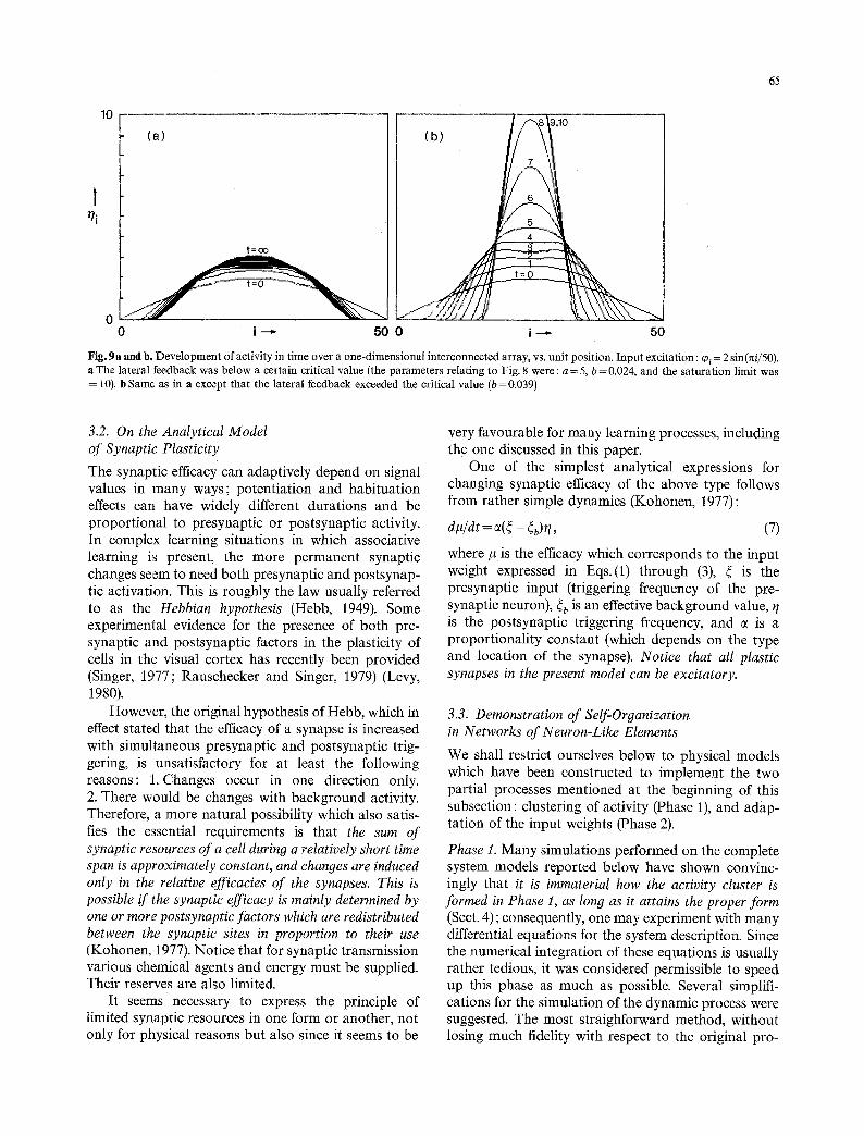
In Fig. ga, the outputs stabilized to values pro- portional t o those of the cO i. The form of the distri- bution changed due to the lateral connections. In Fig. 9b the tli(t) tend to stable clusters which have a lateral extension of the same order of magnitude as the excitatory center in the connectivity function. Such clusters may have a relation to the physiological "columns" of the cortical organization, although here they simply follow from lateral interactions.

It ought to be realized that these clusters are usually self-resetting ; they tend to decay due to habi- tuation, fluctuation of activation, etc.

It should be pointed out that for good clustering the width of the interaction function of Figs. 7 or 8 cannot be very small in relation to the curvature of the input activation. Otherwise, the lateral interaction tends only to enhance the borders of the input acti- vation. Symptoms of such an effect are discernible in Fig. 9b (also Wilson and Cowan, 1973) (see also Sect. 4.3).

65

(a) (b)

t=Co

10[ l-

L i

r/i

' I / - + , B ~ g , + o '

50 0 0 i - - - - i---~ 50

Fig. 9a and b. Development of activity in time over a one-dimensional interconnected array, vs. unit position. Input excitation : ~0~ = 2 sin(nil50). a The lateral feedback was below a certain critical value (the parameters relating to Fig. 8 were: a = 5, b = 0.024, and the saturation limit was = 10). b Same as in a except that the lateral feedback exceeded the critical value (b=0.039)

3.2. On the Analytical Model of Synaptic Plasticity

The synaptic efficacy can adaptively depend on signal values in many ways; potentiation and habituation effects can have widely different durations and be proportional to presynaptic or postsynaptic activity. In complex learning situations in which associative learning is present, the more permanent synaptic changes seem to need both presynaptic and postsynap- tic activation. This is roughly the law usually referred to as the Hebbian hypothesis (Hebb, 1949). Some experimental evidence for the presence of both pre- synaptic and postsynaptic factors in the plasticity of cells in the visual cortex has recently been provided (Singer, 1977; Rauschecker and Singer, 1979) (Levy, 1980).

However, the original hypothesis of Hebb, which in effect stated that the efficacy of a synapse is increased with simultaneous presynaptic and postsynaptic trig- gering, is unsatisfactory for at least the following reasons: 1. Changes occur in one direction only. 2. There would be changes with background activity. Therefore, a more natural possibility which also satis- fies the essential requirements is that the sum of synaptic resources of a cell during a relatively short time span is approximately constant, and changes are induced only in the relative efficacies of the synapses. This is possible if the synaptic efficacy is mainly determined by one or more postsynaptic factors which are redistributed between the synaptic sites in proportion to their use (Kohonen, 1977). Notice that for synaptic transmission various chemical agents and energy must be supplied. Their reserves are also limited.

It seems necessary to express the principle of limited synaptic resources in one form or another, not only for physical reasons but also since it seems to be

very favourable for many learning processes, including the one discussed in this paper.

One of the simplest analytical expressions for changing synaptic efficacy of the above type follows from rather simple dynamics (Kohonen, 1977):

d#/dt = c~(~ - ~b)tl , (7)

where # is the efficacy which corresponds to the input weight expressed in Eqs.(1) through (3), ~ is the presynaptic input (triggering frequency of the pre- synaptic neuron), ~b is an effective background value, t/ is the postsynaptic triggering frequency, and ~z is a proportionality constant (which depends on the type and location of the synapse). Notice that all plastic synapses in the present model can be excitatory.

3.3. Demonstration of Self-Organization in Networks of Neuron-Like Elements

We shall restrict ourselves below to physical models which have been constructed to implement the two partial processes mentioned at the beginning of this subsection : clustering of activity (Phase 1), and adap- tation of the input weights (Phase 2).

Phase 1. Many simulations performed on the complete system models reported below have shown convinc- ingly that it is immaterial how the activity cluster is formed in Phase l, as long as it attains the proper form (Sect. 4) ; consequently, one may experiment with many differential equations for the system description. Since the numerical integration of these equations is usually rather tedious, it was considered permissible to speed up this phase as much as possible. Several simplifi- cations for the simulation of the dynamic process were suggested. The most straighforward method, without losing much fidelity with respect to the original pro-

66

cesses, was to make the increments of tli(t) fairly large at every interval of t, in fact on the order of one decade. Such a speed-up is normal in the discrete-time comput- ing models applied in system theory.

It was then concluded that since the discrimination process is in any case a weIl-estabtished phenomenon, its accurate modelling might not contribute anything essential when contrasted with the more interesting Phase 2. Relying on the results achieved in modelling Phase 1, the solution in each discrimination process (training step) was simply postulated to be some static

function of the input excitations cpi = ~, #u~j. A sim- j = l

ple, although not quite equivalent way, is to in- troduce a threshold by defining a floating bias function 6 common for all units, and then by putting the system equations into a form in which the solution is de- termined implicitly:

l~i=G[q~ i'j- k~S 'k~k--51' + (8)

5 = m a x { ~ 3 - ~-

The nonlinearity o-[. ] might be similar to that applied in Eq. (6), and e is a small positive constant.

Perhaps the simplest model which can still be regarded as physical first performs thresholding of the input excitation and then lets the short-range local feedback amplify the activity and spread it to neigh- bouring units.

cO'i= a[c&- 5], 5= max {~oi} - e , �9 i

rl,= Z 7kO'k. (9) k~S~

All the above equations have been tested to yield roughly similar activity clusters.

Phase 2. The wanted operation in the self2organizing process would be to rotate the weight vectors at each training step in the proper direction. Straightforward application of modifiability law of the type expressed in Eq. (7) would yield an expression

#ij(t q- i ) -~ #ij( t) -F O~rli(t ) (r j -- eb) " (10)

This, however, does not yet involve any normalization. Therefore it must be pointed out that Eq. (7) is already an approximation ; it was in fact derived by postulating that ~#u is constant. Therefore, a more accurate version of Eq. (10) is the following

#o( t + 1) = # , / t ) + ~n / t ) ( r eb) Z [~ij(t) + atli(t) (r - - {b)]' (t 1) J

where normalization based on the conservation of "memory" resources (their linear sum)has been made.

Notice that the factor t/i(t ) in Eqs. (t0) and (11) in fact corresponds to the selection rule relating to Eq. (3); the input weights of only the activated units change. Proportionality to th(t ) further means that the cor- rection becomes a function of distance from the maxi- mum response. However, in addition to rotating the m, vectors, this process still affects their lengths.

It has been pointed out (Oja, 1981) that the factor which is assumed to be redistributed in the "memory" process actually need not be directly proportional to the input weight; for instance, if the input efficacy were proportional to the square root of this factor (a weaker function than the linear one !), then the denominator of Eq. (11) would already become similar to that applied in the teaching rule Eq. (3). Another interesting fact is that the Euclidean norm follows from a simple for- getting law. One may note further that a particular norm, and a particular form of the discrimination function should be related to each other; the most important requirement is to achieve good discrimi- nation between neighbouring responses in one way or another.

Many simulations with physical process models of the above type were carried out; to make them comparable to those performed on the more fictive models of Sect. 2, three-dimensional vectors alone were used. The following adaptive law was then applied:

#it(t) + c%(t) (r eb) (12) ~(t+ 1)= {~=~ 1~/~"

The results were not particularly sensitive to the value of ~b which could be made zero.

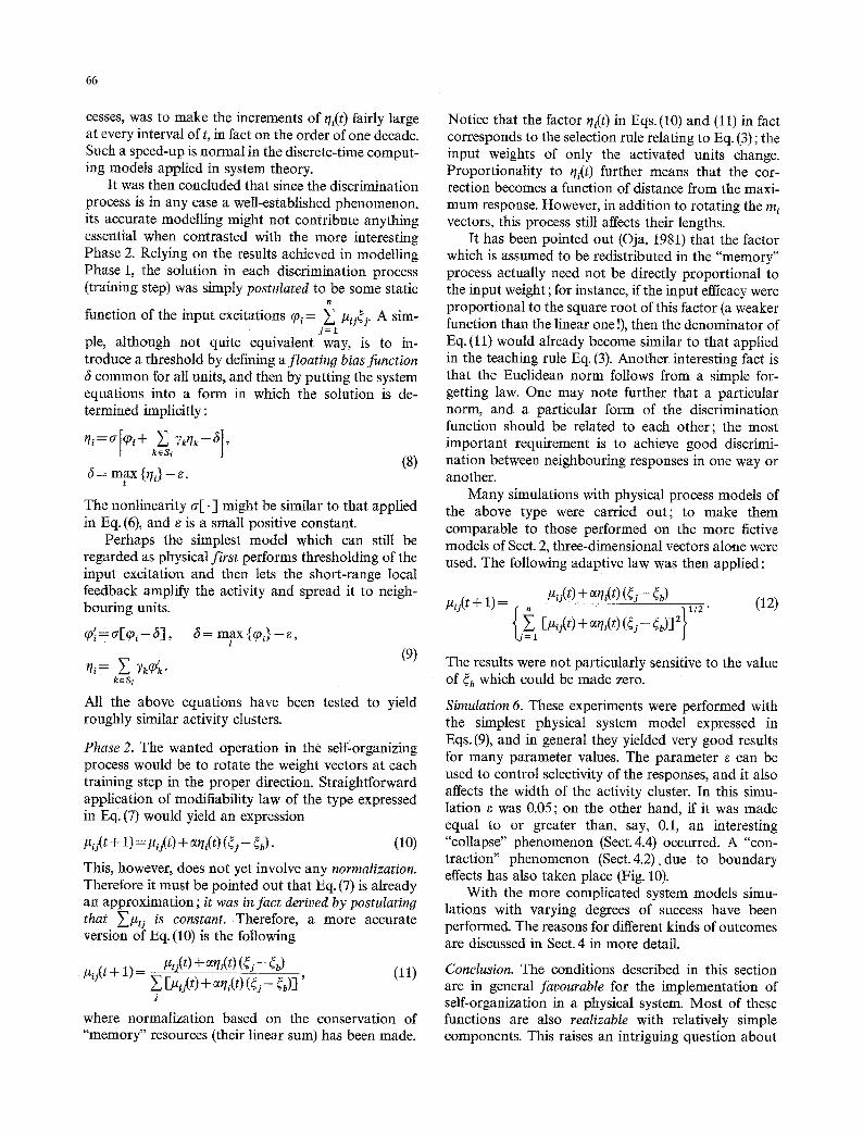
Simulation 6. These experiments were performed with the simplest physical system model expressed in Eqs. (9), and in general they yielded very good results for many parameter values. The parameter e can be used to control selectivity of the responses, and it also affects the width of the activity cluster. In this simu- lation e was 0.05; on the other hand, if it was made equal to or greater than, say, 0.1, an interesting "collapse" phenomenon (Sect. 4.4) occurred. A "con- traction" phenomenon (Sect.4.2).due to boundary effects has also taken place (Fig. 10).

With the more complicated system models simu- lations with varying degrees of success have been performed. The reasons for different kinds of outcomes are discussed in Sect. 4 in more detail.

Conclusion. The conditions described in this section are in general favourable for the implementation of self-organization in a physical system. Most of these functions are also realizable with relatively simple components. This raises an intriguing question about

i~ :,'~-~.. '~ X "~ ~,'.~ ~.-,',xyC:~ \

la ) (b)

Fig. 10. a Distribution of training vectors used in a simple physical system model, b Distribution of weight vectors m~ after 4000 training steps

the realizability of this phenomenon in the neural networks. At least if one does not stipulate that the exact mathematical expression should be valid, but allows some variance, which in any case retains certain necessary conditions (good discrimination between neighbouring responses and formation of activity clus- ters in one way or another), the conditions met in neural circuits could also be conducive to this phenomenon.

4. Some Special Effects

4.1. The Magnification Factor

In this subsection an important property characteristic of biological organisms will be demonstrated: the scale or magnification factor of the map is usually not constant but a function of location in the array which depends on the frequency of input events that have mapped into that location during adaptation. It seems that the magnification factor is approximately pro- portional to the above frequency; this me,ins that the network resources are utilized optimally in accordance with need.

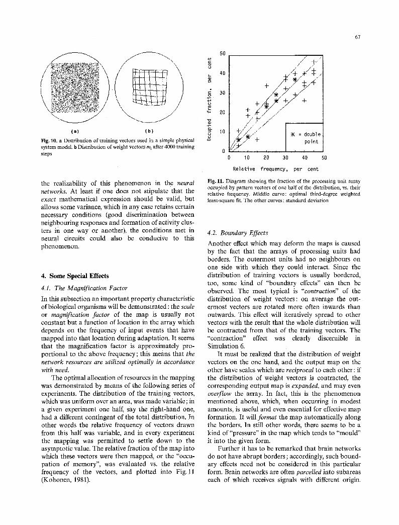
The optimal allocation of resources in the mapping was demonstrated by means of the following series of experiments. The distribution of the training vectors, which was uniform over an area, was made variable; in a given experiment one half, say the right-hand one, had a different contingent of the total distribution, h other words the relative frequency of vectors drawn from this half was variable, and in every experiment the mapping was permitted to settle down to the asymptotic value. The relative fraction of the map into which these vectors were then mapped, or the "occu- pation of memory", was evaluated vs. the relative frequency of the vectors, and plotted into Fig. 11 (Kohonen, 1981).

67

50

o o

40

: 30 o ~s u

4- 20

"~- I 0 o

/ " ~ i . / ,i" _....

g,r Y y.4 .... /.~ ..,.-"" ~.,,/"

+ / " + / +

-i-/4:- ..,,,~ ...,.."

~:'::::.,~,."/" ~ = double + . . . . oo :

0 I 0 20 30 40 50

Relative frequency, per cent

Fig. 11. Diagram showing the fraction of the processing unit array occupied by pattern vectors of one half of the distribution, vs. their relative frequency. Middle curve: optimal third-degree weighted least-square fit. The other curves: standard deviation

4.2. Boundary Effects

Another effect which may deform the maps is caused by the fact that the arrays of processing units had borders. The outermost units had no neighbours on one side with which they could interact. Since the distribution of training vectors is usually bordered, too, some kind of "boundary effects" can then be observed. The most typical is "contraction" of the distribution of weight vectors: on average the o u t - ermost vectors are rotated more often inwards than outwards. This effect will iteratively spread to other vectors with the result that the whole distribution will be contracted from that o f the training vectors. The "contraction" effect was clearly discernible in Simulation 6.

It must be realized that the distribution of weight vectors on the one hand, and the output map on the other have scales which are reciprocal to each other : if the distribution of weight vectors is contracted, the corresponding output map is expanded, and may even overflow the array. In fact, this is the phenomenon mentioned above, which, when occurring in modest amounts, is useful and even essential for effective map formation. It will format the map automatically along the borders. In still other words, there seems to be a kind of "pressure" in the map which tends to "mould" it into the given form.

Further it has to be remarked that brain networks do not have abrupt borders ; accordingly, such bound- ary effects need not be considered in this particular form. Brain networks are often parcelled into subareas each of which receives signals with different origin.

68

Ordering within each subarea may thus occur inde- pendently and be only slightly affected at the de- marcation zones.

4.3. The "Pinch" Phenomenon

Although the type of self-organization reported in this paper is not particularly "brittle" with respect to parameters, conditions in which this process fails do exist. One of the typical effects encountered is termed the "'pinch" phenomenon. This means simply that the distribution of the memory vectors does not spread out into a planar configuration, but is instead concentrated onto a ring. Some kind of one-dimensional order of vectors may be discernible along the perimeter of the ring which, however, does not produce a meaningful map in the processing unit array.

A typical condition for the "pinch" phenomenon is poor selectivity in the discrimination process, especially when the range of lateral interaction is too short. This results in several "peaks" of activity, usually at the opposite edges of the array. In consequence, con- tradictory corrections are imposed on the weight vectors. Figure 12 exemplifies a typical distribution of weight vectors (shown without lattice lines) when this effect was fully developed.

4.4. The "Collapse" Phenomenon

Another pitfall related to the "pinch" phenomenon, and not much different in principle from the con- traction effect discussed in Sect. 4.2, should be men- tioned. This is the outcome in which all weight vectors tend to attain the same value. This is termed "collapse" (of the distribution, not of the map). This phenomenon was observed when the range of lateral interaction was too long. For instance, a too low threshold in the models of Sect. 3.4 resulted in the "collapse".

This effect is manifested in the output responses so that large groups of units give the same response.

,? ... " % . /

) \

Fig. 12. An example of a weight vector distribution when the "pinch" phenomenon was due

4.5. The "Focusing" Phenomenon

This case is opposite to the "collapse". It may happen that one or more array units take over, i.e., they become sensitized to large portions of the distribution of the training vectors. In this case there is usually no order in the mapping. This failure is mainly due to poor general design or malfunction of the system, especially if the lateral interaction between neighbouring elements is too weak. Another common reason is that the normalization of the weight vectors is not done in a proper way whereby discrimination between the re- sponses of neighbouring units becomes impossible.

5. On the Possible Roles of Various Neural Circuits Made by Interneurons

In view of the effects reported in Sects. 4.1 through 4.4 now seems possible to draw conclusions about the meaning of certain structures met in neural networks. Throughout the history of neuroanatomy and neu- rophysiology there has been much speculation about the purpose of the polysynaptic circuits made by various interneurons in CNS structures. Some in- vestigators seem to be searching for an explanation in terms of complex computational operations while others see the basic implementation of feature de- tectors for sensory signals in these circuits. There are, e.g., quite specific circuits made by some cells such as the bipolar, chandelier, and basket cells in the cortex, for which a more detailed explanation is needed.

However, the roles of the above-mentioned cells, as well as the characteristic ramification of the axon collaterals of most cortical cell types would become quite obvious if the purpose was to implement a neural network with a capacity for predominantly two- dimensional self-organization. The bipolar cells, the recurrent axon collaterals of various cells, and the general vertical texture of the cortex warrant a high degree of conductance and spreading of signal activity in the vertical direction. On the other hand, if it were necessary to implement a lateral interaction, such as that described by the excitation function of the type delineated in Fig. 8a, then the stellate, basket, chan- delier, etc. interneurons, and the horizontal intracorti- cal axon collaterals would account for the desired lateral coupling.

The effects reported in Sects.4.1 through 4.4 in- dicate that although self-organization of this type is not a particularly "brittle" phenomenon, the form of the lateral interaction function needs some adjustment. In a neural tissue this must be done by active circuits for which the interneurons are needed.

It might even be said that the fraction of a certain cell type in the composition of all neurons is a tuning

69

parameter by which an optimal form of local interaction can be defined. The characteristic branchings of a particular cell type may roughly serve a similar pur- pose to that of the different basis functions in ma- thematical functional expansions. This conception is also in agreement with the fact that all cell types are not present in different species, or even in different parts of the brain: for some purposes it may be sufficient to "tune" a certain interaction with fewer types of cell ("basis functions"), while for more exacting tasks a richer variety of cells would be needed. Such recruitment of new forms according to need would be in complete agreement with the general principles of evolution.

References

Amari, S.-I. : Topographic organization of nerve fields. Bull. Math. Biol. 42, 339-364 (1980)

Hebb, D. : Organization of behavior. New York: Wiley 1949 Kohonen, T. : Associative memory - a system-theoretical approach.

Berlin, Heidelberg, New York: Springer 1977, 1978 Kohonen, T. : Automatic formation of topological maps of patterns

in a self-organizing system. In : Proc. 2rid Scand. Conf. on Image Analysis, pp. 214-220, Oja, E., Simula, O. (eds.). Espoo : Suomen Hahmontunnistustutkimuksen Seura 1981

Levy, W. : Limiting characteristics of a candidate elementary me- mory unit: LTP studies of entorhinal-dentate synapses. (To appear in a book based on the workshop "Synaptic modifi- cation, neuron selectivity, and nervous system organization",

" Brown University, Rhode Island, Nov. 16-19, 1980) Lynch, G.S., Rose, G., Gall, C.M. : In: Functions of the septo-

hippocampal system, pp. 5-19. Amsterdam: Ciba Foundation, Elsevier 1978

Malsburg, Ch. yon der: Self-organization of orientation sensitive cells in the striate cortex. Kybernetik 14, 85-100 (1973)

Malsburg, Ch. vonder , Willshaw, D.J. : How to label nerve cells so that they can interconnect in an ordered fashion. Proc. Natl. Acad. Sci. USA 74, 5176-5178 (1977)

Mountcastle, V.B. : Modality and topographic properties of single neurons of cat's somatic sensory cortex. J. Neurophys. 20, 408-434 (1957)

Oja, E.: A simplified neuron model as a principal component analyzer (1981) (to be published)

Rauschecker, J.P., Singer, W. : Changes in the circuitry of the kitten's visual cortex are gated by postsynaptic activity. Nature 280, 58-60 (1979)

Reale, R.A., Imig, T.J. : Tonotopic organization in auditory cortex of the cat. J. Comp. Neurol. 192, 265-291 (1980)

Rosenblatt, F. : Principles of neurodynamics: Perceptrons and the theory of brain mechanisms. Washington, D.C. : Spartan Books 1961

Singer, W., Rauschecker, J., Werth, R. : The effect of monocular exposure to temporal contrasts on ocular dominance in kittens. Brain Res. 134, 568-572 (1977)

Swindale, N.V. : A model for the formation of ocular dominance stripes. Proc. R. Soc. B208, 243-264 (1980)

Towe, A. : Notes on the hypothesis of columnar organization in somatosensory cerebral cortex. Brain Behav. Evol. 11, 16-47 (1975)

Willshaw, D.J., Malsburg, Ch. yon der: How patterned neural connections can be set up by self-organization. Proc. R. Soc. B194, 431-445 (1976)

Willshaw, D.J., Malsburg, Ch. yon der: A marker induction mecha- nism for the establishment of ordered neural mappings; its application to the retino-tectal problem. Phil. Trans. R. Soc. Lond. B287, 203-243 (!:979)

Wilson, H.R., Cowan, J.D. : A mathematical theory of the functional dynamics of cortical and thalamic nervous tissue. Kybernetik 13, 55-80 (1973)

Received: July 25, 1981

Prof. Dr. Teuvo Kohonen Department of Technical Physics Helsinki University of Technology SF-02150 Espoo 15 Finland