Embed Size (px)
Citation preview
International Journal of InnovativeComputing, Information and Control ICIC International c⃝2012 ISSN 1349-4198Volume 8, Number 3(A), March 2012 pp. 1955–1971
SELF-ORGANIZING FUZZY RADIAL BASIS FUNCTIONNEURAL-NETWORK CONTROLLER FOR ROBOTIC
MOTION CONTROL
Ruey-Jing Lian1,∗ and Chung-Neng Huang2
1Department of Management and Information TechnologyVanung University
No. 1, Wanneng Rd., Jhongli City, Toayuan County 32061, Taiwan∗Corresponding author: [email protected]; [email protected]
2Graduate Institute of Mechatronic System EngineeringNational University of Tainan
No. 33, Sec. 2, Shu-Lin St., Tainan 70005, [email protected]; [email protected]
Received December 2010; revised April 2011
Abstract. Robotic systems are complicated, nonlinear, multiple-input multiple-output(MIMO) systems, which make the design of model-based controllers for robotic systemsparticularly difficult. Moreover, to achieve reasonable control performance, the dynamiccoupling effects between degrees of freedom (DOFs) of the robotic systems must be over-come during the control process. Although a model-free, self-organizing fuzzy controller(SOFC) can be applied to the manipulation of complex and nonlinear systems, its pa-rameters are difficult to select appropriately, and it mainly focuses on controlling single-input single-output systems rather than MIMO systems. To address these problems, thisstudy developed a self-organizing fuzzy radial basis function neural-network controller(SFRBFNC) for robotic systems. The SFRBFNC introduces a radial basis functionneural-network into the SOFC to compensate for the dynamic coupling effects between theDOFs of the robotic system, as well as solve the problem caused by inappropriate selectionof parameters in designing an SOFC. The SFRBFNC demonstrated control performancesuperior to the SOFC, as shown in experimental results from motion control tests of a6-DOF robot.Keywords: Multiple-input multiple-output (MIMO) systems, Radial basis functionneural-network, Robotic motion control, Self-organizing fuzzy controller (SOFC)
1. Introduction. Research and development of industrial automation are important toimprove productivity and quality. The robot is one of the most effective machines usedin industrial automation. Flexible multifunctional robots are ideal candidates to replacehumans for high-risk jobs in unsafe environments or those requiring repetitive motions.The design of the controller for robotic trajectory motion needs to be efficient and accuratesince many industrial applications require robots to perform tasks with high precision.Robots are complicated, nonlinear, multiple-input multiple-output (MIMO) systems. Itis difficult to design model-based controllers to manipulate such systems. Thus, it isnecessary to develop model-free control strategies for the control of complex and nonlinearrobots.
Fuzzy logic control, which does not require a mathematical model of the system, hasbeen successfully applied to robotic systems to improve their control performances [1-3]. However, a fuzzy logic controller (FLC) for practical applications has difficulties indetermining suitable membership functions and fuzzy rules. Moreover, the main problem
1955
1956 R.-J. LIAN AND C.-N. HUANG
in the design of an FLC is that both the inference table and the knowledge base of the FLC,which are constructed using an expert’s knowledge or the experience of a skilled operator,are fixed after selection. To solve the problems of the FLC implementation, Procyk andMamdani [4] first proposed a self-organizing fuzzy controller (SOFC). This control strategyinvolves the use of online learning, rather than human thinking, to establish fuzzy controlrules, thereby simplifying the procedures for designing an FLC. Subsequently, Shao [5]and Zhang and Edmunds [6] developed modified learning methods to further simplify thedesign of the SOFC. However, the construction of the modified learning scheme is basedon a performance decision table proposed by Procyk and Mamdani [4] and the design ofa performance decision table is as difficult as the design of a fuzzy rule table. Therefore,to overcome this problem, Yang [7], Huang and Lee [8], and Lin and Lian [9,10] used theoutput error and the error change of the system to establish a learning algorithm thatcan adjust the linguistic fuzzy rule table of the SOFC directly, so that it can be generatedwithout any initial fuzzy rules. The SOFC eliminates the difficulty of finding appropriatemembership functions and fuzzy rules in designing an FLC. Under the disk operatingsystem, Huang and Lee [8] employed this SOFC to control a robot with 5 degrees offreedom (DOFs) and evaluated its trajectory tracking performance.The SOFC has demonstrated its superior learning ability in controlling complicated
and nonlinear systems in practical applications [8-10]; however, both the learning rate andweighting distribution in the SOFC must be carefully chosen and are fixed once selected.Unfortunately, inappropriate selection of either the weighting distribution or the learningrate (or both) in the SOFC will substantially affect the output response of the systemand may result in an unstable system. Moreover, the SOFC is primarily designed forcontrolling single-input single-output systems, so the use of the SOFC to control roboticsystems, which are MIMO systems, cannot eliminate the dynamic coupling effects betweenthe DOFs of the robotic systems.Neural networks for robotic system control have attracted the attention of many re-
searchers because they have model-free features and learning abilities. Neural networkshave been used to control complicated robotic systems and their control performanceshave been demonstrated in previous studies [11,12]. However, in practical applications,convergence rates of neural networks are too slow to compensate for the dynamic couplingeffects between the DOFs of robotic systems. Noticeably, it is difficult to achieve satisfac-tory control performance when using a neural network to control robotic systems, unlessthe convergence algorithm and the training speed of the neural network are significantlyimproved.The design and implementation of fuzzy control systems with learning capacities in-
troduced by neural networks have become very active areas of research in recent years[13-15]. Such a synergism between neural networks and fuzzy logic systems, integratedinto a functional system, has provided a new way of realizing intelligent systems for var-ious applications. Most of the hybrid fuzzy-logic and neural network control strategiesmake use of neural networks to determine the membership functions and use the deter-mined membership functions to design appropriate fuzzy control rules, which are fixedonce decided. Nevertheless, the design of these control strategies is very complicated andimpractical for practical industrial applications. The robot is an example of an MIMOsystem. It is characterized by complicated dynamic coupling effects between the DOFs ofthe robot. Controller development for robotic systems needs to overcome these couplingeffects to improve the overall control performances. However, in implementing robotic sys-tem control, few considerations [16,17] are usually entertained to deal with the dynamiccoupling effects between the DOFs of robotic systems.
FUZZY RADIAL BASIS FUNCTION NEURAL-NETWORK CONTROLLER 1957
As mentioned previously, when the SOFC is used to handle robotic systems, its param-eters are difficult to choose appropriately and the dynamic coupling effects between theDOFs of the robotic systems cannot be improved. To eliminate the problem, this study de-velops a self-organizing fuzzy radial basis function neural-network controller (SFRBFNC)for robotic systems. The SFRBFNC introduces a radial basis function neural-network(RBFN) [18-20], as the training algorithm of a neural network, into an SOFC to com-pensate for the dynamic coupling effects between the DOFs of the robotic system andovercome the problem encountered by the SOFC with inappropriately selected parame-ters. Therefore, the use of the SFRBFNC to manipulate robotic systems not only solvesthe problem of an SOFC implementation, but also alleviates the dynamic coupling effectsbetween the DOFs of the robotic systems. Most of the work in this field involves computersimulations of simple robotic system models. This study explores the control performanceof the SFRBFNC for motion control of a 6-DOF robot experimentally.
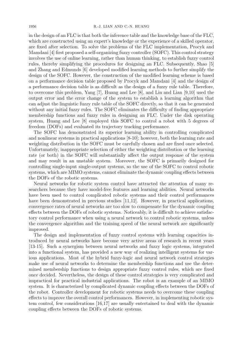
2. Robotic System. A 5-DOF robot (type RV-MI), made by the Mitsubishi Company,had sliding track equipment added to its bottom in order to increase its horizontal move-ment capability and expand its workspace. Moreover, the robot was retrofitted, allowingan individual to use a personal-computer-based controller to control it. The retrofittedrobot has 6 DOFs and each of its joints is driven by a direct current servo-motor.
6-DOF Robot
Interface Card
PCI-8136
D/A
DI
Motor
Driver
Encoder
Transformation
Circuit
Limit
Switch
DecoderPentium IV
2.6 GHz
Personal
Computer
Figure 1. Experimental set-up of the retrofitted robotic control system.Digital-to-analog (D/A); digital-input (DI)
Figure 1 presents an experimental set-up of the retrofitted robotic control system. Toevaluate the performance of the proposed controller for the control of the robotic system,an appropriate reference trajectory was first planned to convert the points θi(k) into acontinuously desired trajectory θri(k). This study used the joint-space trajectory for acubic interpolation polynomial [21] to plan the desired smooth motion for each joint ofthe robot.
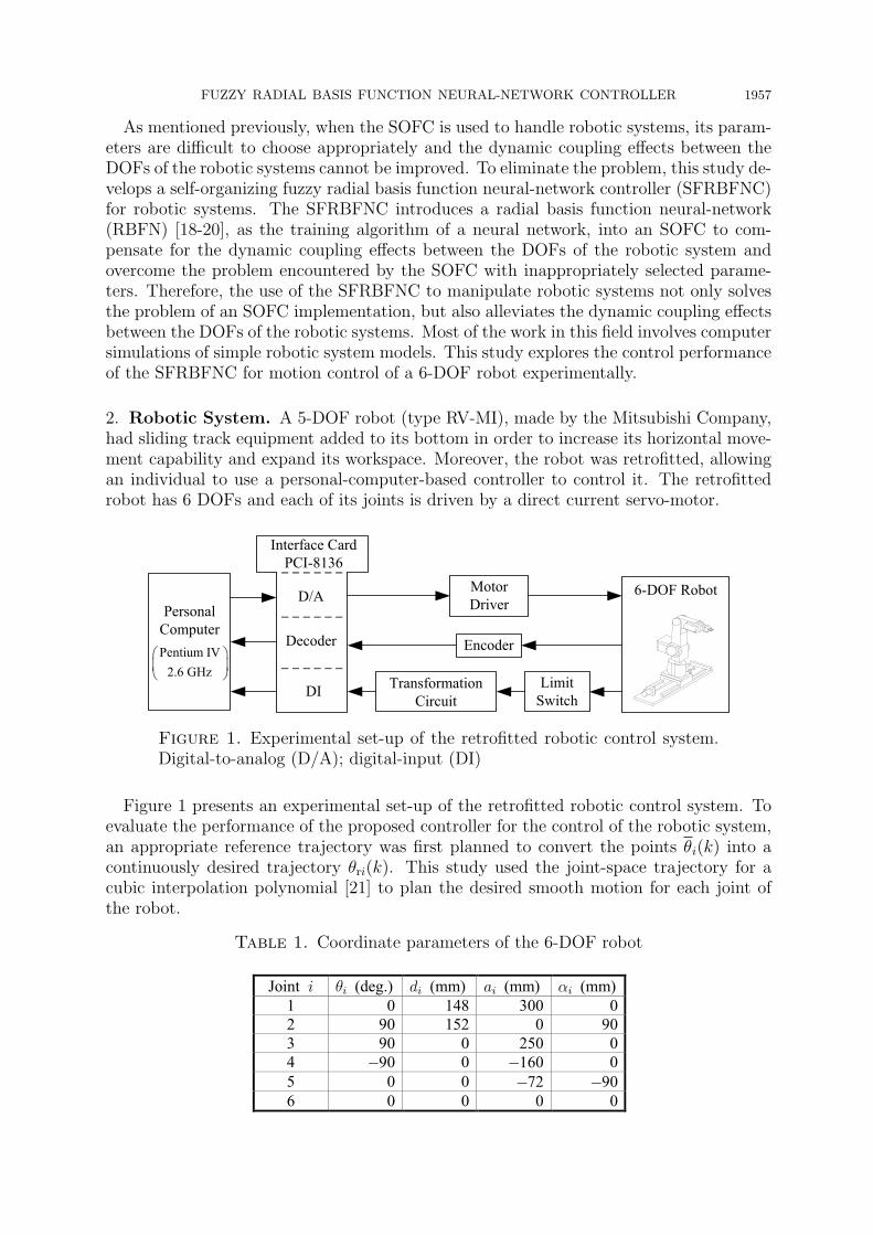
Table 1. Coordinate parameters of the 6-DOF robot
Joint i µi (deg.) di (mm) ai (mm) ®i (mm)
1 0 148 300 0
2 90 152 0 90
3 90 0 250 0
4 ¡90 0 ¡160 0
5 0 0 ¡72 ¡90
6 0 0 0 0
1958 R.-J. LIAN AND C.-N. HUANG
(a)
replacements
X0
Y0
Z0
X1
Y1
Z1
X2
Y2
Z2
X3
Y3
Z3
X4
Y4
Z4
X5
Y5
Z5 X6
Y6
Z6
a 1
a3
a4
a5
d1
d2
(b)
Figure 2. Coordinate system of the 6-DOF robot
Figure 2 shows the defined coordinate system and the joint parameters for the 6-DOFrobot using the Denavit-Hartenberg (D-H) indicative method [22]. To determine thecontrol performance of the robotic trajectory tracking, the kinematics equation and theinverse kinematics equation are first established for the relationship between the joint-space and the Cartesian-space. The joint parameters, defined as per the rules establishedby the D-H representation, are listed in Table 1. Similar to the derived process from Fuet al. [22] and Huang and Lian [16], the kinematics equation and the inverse kinematicsequation of the 6-DOF robot can be determined.The 6-DOF robotic system, in this study, exhibits nonlinear, time-varying characteris-
tics because of backlash, friction, Coriolis coupling, gravity force, saturation of the actu-ator, and other factors. Traditional model-based controllers are difficult to implement onthis complex robotic system. Although a model-free SOFC can be employed to controlsuch systems, its learning rate and weighting distribution are arduous to select appropri-ately. When the SOFC with inappropriately chosen parameters is used to manipulate arobotic system, it may excessively modify its fuzzy rules during the control process so thatthe system’s output response generally results in oscillatory phenomena or becomes un-stable. In addition, the use of the SOFC to handle robotic systems, the dynamic couplingeffects between the DOFs of the robotic systems cannot be compensated. To solve theseproblems, this study developed an SFRBFNC to control the 6-DOF robot for improvingthe control performance of the robot.
3. Controller Design.
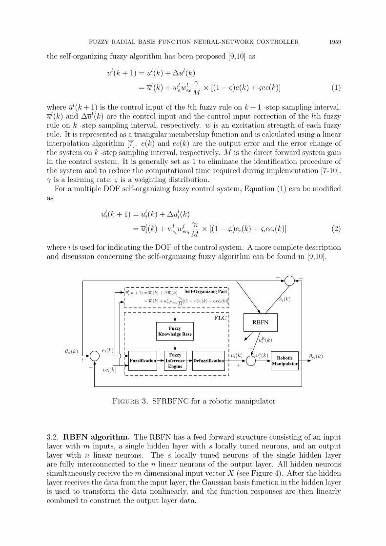
3.1. Self-organizing fuzzy algorithm. The self-organizing part is introduced into anFLC to constitute an SOFC, as depicted in Figure 3, and consists of three steps: perfor-mance measure, model estimation, and rule modification [7-10]. A generalized form for
FUZZY RADIAL BASIS FUNCTION NEURAL-NETWORK CONTROLLER 1959
the self-organizing fuzzy algorithm has been proposed [9,10] as
ul(k + 1) = ul(k) + ∆ul(k)
= ul(k) + wlew
lec
γ
M× [(1− ς)e(k) + ςec(k)] (1)
where ul(k+1) is the control input of the lth fuzzy rule on k+1 -step sampling interval.ul(k) and ∆ul(k) are the control input and the control input correction of the lth fuzzyrule on k -step sampling interval, respectively. w is an excitation strength of each fuzzyrule. It is represented as a triangular membership function and is calculated using a linearinterpolation algorithm [7]. e(k) and ec(k) are the output error and the error change ofthe system on k -step sampling interval, respectively. M is the direct forward system gainin the control system. It is generally set as 1 to eliminate the identification procedure ofthe system and to reduce the computational time required during implementation [7-10].γ is a learning rate; ς is a weighting distribution.
For a multiple DOF self-organizing fuzzy control system, Equation (1) can be modifiedas
uli(k + 1) = ul
i(k) + ∆uli(k)
= uli(k) + wl
eiwl
eci
γiM
× [(1− ςi)ei(k) + ςieci(k)] (2)
where i is used for indicating the DOF of the control system. A more complete descriptionand discussion concerning the self-organizing fuzzy algorithm can be found in [9,10].
Fuzzy
Knowledge Base
Fuzzy
Inference
Engine
DefuzzificationFuzzification
Self-Organizing Part
Robotic
Manipulator
µri(k)ui(k) µyi(k)
ei(k)
eci(k)
uli(k + 1) = ul
i(k) + ¢uli(k)
= uli(k) + wl
eiwl
eci
°i
M[(1¡ &i)ei(k) + &ieci(k)]
+
FLC
¡
RBFN
uRi (k)
u?i (k)
+
+
+¡
ei(k)
Figure 3. SFRBFNC for a robotic manipulator
3.2. RBFN algorithm. The RBFN has a feed forward structure consisting of an inputlayer with m inputs, a single hidden layer with s locally tuned neurons, and an outputlayer with n linear neurons. The s locally tuned neurons of the single hidden layerare fully interconnected to the n linear neurons of the output layer. All hidden neuronssimultaneously receive the m-dimensional input vector X (see Figure 4). After the hiddenlayer receives the data from the input layer, the Gaussian basis function in the hidden layeris used to transform the data nonlinearly, and the function responses are then linearlycombined to construct the output layer data.
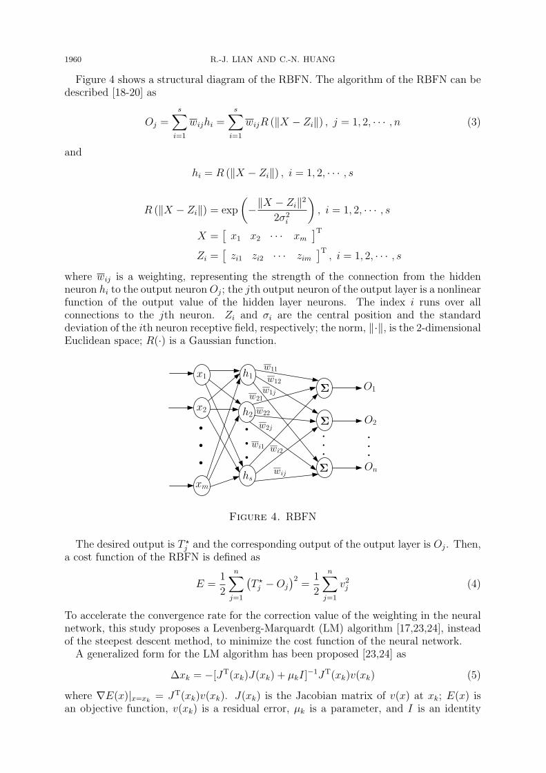
1960 R.-J. LIAN AND C.-N. HUANG
Figure 4 shows a structural diagram of the RBFN. The algorithm of the RBFN can bedescribed [18-20] as
Oj =s∑
i=1
wijhi =s∑
i=1
wijR (∥X − Zi∥) , j = 1, 2, · · · , n (3)
and
hi = R (∥X − Zi∥) , i = 1, 2, · · · , s
R (∥X − Zi∥) = exp
(−∥X − Zi∥2
2σ2i
), i = 1, 2, · · · , s
X =[x1 x2 · · · xm
]TZi =
[zi1 zi2 · · · zim
]T, i = 1, 2, · · · , s
where wij is a weighting, representing the strength of the connection from the hiddenneuron hi to the output neuron Oj; the jth output neuron of the output layer is a nonlinearfunction of the output value of the hidden layer neurons. The index i runs over allconnections to the jth neuron. Zi and σi are the central position and the standarddeviation of the ith neuron receptive field, respectively; the norm, ∥·∥, is the 2-dimensionalEuclidean space; R(·) is a Gaussian function.
•••
•••
•••
w11
w12
w1jw21
w22
w2j
wi1
wij
wi2
x1
x2
xm
On
O2
O1
h2
h1
hs
§
§
§
•••
Figure 4. RBFN
The desired output is T ⋆j and the corresponding output of the output layer is Oj. Then,
a cost function of the RBFN is defined as
E =1
2
n∑j=1
(T ⋆j −Oj
)2=
1
2
n∑j=1
v2j (4)
To accelerate the convergence rate for the correction value of the weighting in the neuralnetwork, this study proposes a Levenberg-Marquardt (LM) algorithm [17,23,24], insteadof the steepest descent method, to minimize the cost function of the neural network.A generalized form for the LM algorithm has been proposed [23,24] as
∆xk = −[JT(xk)J(xk) + µkI]−1JT(xk)v(xk) (5)
where ∇E(x)|x=xk= JT(xk)v(xk). J(xk) is the Jacobian matrix of v(x) at xk; E(x) is
an objective function, v(xk) is a residual error, µk is a parameter, and I is an identity
FUZZY RADIAL BASIS FUNCTION NEURAL-NETWORK CONTROLLER 1961
matrix. The LM algorithm has a very useful feature. It approaches the steepest descentalgorithm with a small convergence rate as µk is increased,
xk+1 = xk −1
µk
JT(xk)v(xk) = xk −1
µk
∇E(x) for large µk (6)
When µk is decreased to zero, the LM algorithm becomes a Gauss-Newton method. TheLM algorithm begins from a small µk value (such as µk = 0.01). If a step does not yield asmaller value for E(x), the step will be repeated with µk multiplied by some factor η > 1(such as η = 10). Ultimately, E(x) should be reduced because a small step is taken inthe direction of the steepest descent. If a step does not produce a smaller value for E(x),µk will be divided by η for the next step. This is done so that the LM algorithm willapproach the Gauss-Newton method, which should provide faster convergence [23].
According to Equations (3)-(6), the weighting correction (∆wij), central position cor-rection (∆Zi), and standard deviation correction (∆σi) of the RBFN can be separatelydetermined as
∆wij = −[J(wij)
TJ(wij) + µkI]−1
JT(wij)vj(wij) (7)
∆Zi = −[J(Zi)
TJ(Zi) + µkI]−1
JT(Zi)vj(Zi) (8)
∆σi = −[J(σi)
TJ(σi) + µkI]−1
JT(σi)vj(σi) (9)
The output value of the RBFN has to be maintained within an appropriate range forthis control strategy implementation, so a nonlinear transformation layer is introducedbetween the hidden layer and the output layer of the RBFN to regulate the output valueof the RBFN to achieve the aforementioned goal. The procedure for determining theweighting correction ∆wij of the nonlinear transformation layer is similar to the procedurefor determining that of the RBFN between the hidden layer and the output layer.
To derive the weighting correction of the aforementioned RBFN, a batch learningmethod [25] was employed and an objective function of the RBFN for the step p wasdefined as
E⋆p =
1
2
∑j
(θrpj − θypj)2 =
1
2
∑j
e2pj (10)
where θrpj and θypj express the desired set-points and the system outputs in the stepp, respectively. When E⋆
p approaches zero, the mapping between inputs and outputs ofeach step p is realized. Similar to the derived process of Equations (7)-(9), the weightingcorrection, central position correction, and standard deviation correction of the RBFN inthe step p can be individually determined as
∆wij = −∑p
[Jp(wij)
TJp(wij) + µkpI]−1
JTp (wij)epj(wij)
∆Zi = −∑p
[Jp(Zi)
TJp(Zi) + µkpI]−1
JTp (Zi)epj(Zi)
∆σi = −∑p
[Jp(σi)
TJp(σi) + µkpI]−1
JTp (σi)epj(σi)
If the input data at k -step is X(k), the updated rules for the aforementioned correctionscan be separately described as
wij(k + 1) = wij(k) + ∆wij(k) (11)
Zi(k + 1) = Zi(k) + ∆Zi(k) (12)
σi(k + 1) = σi(k) + ∆σi(k) (13)
1962 R.-J. LIAN AND C.-N. HUANG
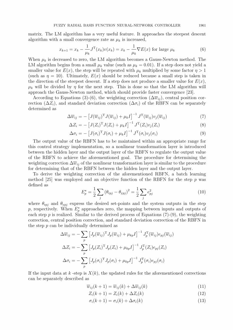
3.3. Design of an SFRBFNC. The SOFC is composed of a self-organizing part and anFLC, as shown in Figure 3. Its learning algorithm was presented in the preceding section.Design procedure of an FLC is described here. The structure of an FLC design consistsof the following: the definition of input-output fuzzy variables, decision-making related tofuzzy control rules, fuzzy inference logic, and defuzzification. From Figure 3, the controlvariables of the system are defined as
ei(k) = θri(k)− θyi(k) (14)
eci(k) = ei(k)− ei(k − 1) (15)
where ei(k) and ei(k − 1) are the output errors of the system on k -step and k − 1 -step sampling intervals, respectively; eci(k) is the error change of the system on k -stepsampling interval; θri(k) and θyi(k) represent the reference input and the output responseof the system on k -step sampling interval respectively. The subscript (i = 1, 2, . . . , 5) isemployed to represent each joint of the robot.A triangular membership function, depicted in Figure 5, is employed to convert these
input variables (ei(k) and eci(k)) and the output variable (ui(k)) into linguistic controlvariables (NB, NM, . . ., PB), where βj
i is a scaling factor. The subscript i has beendescribed previously. The superscript (j = 1, 2, 3) is used to express the system’s outputerror, error change, and control input.
NB NM NS PS PM PBZO
1
0¡6¯j
i ¡4¯j
i ¡2¯j
i 2¯j
i 4¯j
i 6¯j
i
Figure 5. Membership function of the FLC. Negative big (NB), negativemedium (NM), negative small (NS), positive big (PB), positive medium(PM), positive small (PS), and zero (ZO)
This study employed fuzzy control rules of the state evaluation [26] for controlling theinherently complicated and nonlinear robot. To prevent the change of the antecedentsuitability of the fuzzy-inference logic to be unsmooth, the fuzzy-inference logic used analgebraic product [27], instead of the Max−Min product composition [26], to operatethe fuzzy rules. Finally, this study applied the height method [26] to defuzzify the outputvariables to obtain accurate control inputs for controlling this system. The aforemen-tioned design process yields the following actual control input of the actuator for thisself-organizing fuzzy control system,
ui(k) = ui(k − 1) + ∆ui(k) (16)
where ∆ui(k) indicates the control input increment of the system on k -step samplinginterval. ui(k) and ui(k − 1) represent the control inputs of the system on k -step andk − 1 -step sampling intervals, respectively.Figure 3 shows an SFRBFNC for a robotic manipulator, in which the variables of the
input layer of the RBFN are θri(k) and ei(k). The variable of the output layer of theRBFN is uR
i (k), which represents the control effort generated from the RBFN operation,to compensate for the dynamic coupling effects between the DOFs of the robotic systemand to solve the problem caused by the inappropriate selection of the parameters in
FUZZY RADIAL BASIS FUNCTION NEURAL-NETWORK CONTROLLER 1963
designing an SOFC. Accordingly, the total control input of each DOF of a robotic systemu⋆i (k), obtained by combining an SOFC with an RBFN, can be represented as
u⋆i (k) = ui(k) + uR
i (k) (17)
Moreover, it is important to determine the stability and robustness of the proposedcontroller for control applications. However, the stability and robustness of the SFRBFNCare difficult to demonstrate using a rigorously mathematical proof. This is because theproof requires complex mathematical operations and might be impossible to obtain atpresent. One of the methods such as the state-space approach [17], which does not needcomplicated mathematical operations, can be employed to determine the stability androbustness of the proposed controller. Therefore, the stability and robustness of theSFRBFNC can be demonstrated and guaranteed by following the derived process fromLin and Lian [17] using the state-space approach.
4. Experimental Results. Figure 1 presents an experimental set-up of the retrofittedrobotic control system. This retrofitted robot was controlled using a compatible IBMPC Pentium IV (2.6 GHz) central processing unit for processing all of the system input-output data, as well as the control parameters. The requisite interface is a PCI-8136card comprising a digital-to-analog part with 6 channels, an analog-to-digital part with 6channels, a digital-input part with 19 channels, and 6 decoding channels. The card camefrom the ADLINK Company.
This study introduced an RBFN into the SOFC to construct an SFRBFNC for roboticsystems. To conveniently manipulate the robotic manipulator in practical industrial ap-plications, a controller with a friendly graphical-user-interface (GUI) should be developed.To achieve this goal, this study used the Borland C++ Builder programming language tocode the proposed controllers (SOFC and SFRBFNC) with friendly GUIs. The codingand the experimental tests were done under a Windows XP operating system.
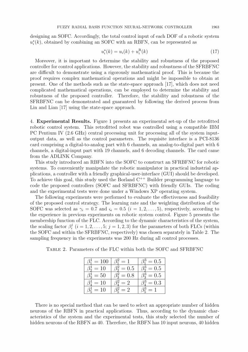
The following experiments were performed to evaluate the effectiveness and feasibilityof the proposed control strategy. The learning rate and the weighting distribution of theSOFC was selected as γi = 0.7 and ςi = 0.5 (i = 1, 2, . . . , 5), respectively, according tothe experience in previous experiments on robotic system control. Figure 5 presents themembership function of the FLC. According to the dynamic characteristics of the system,the scaling factor βj
i (i = 1, 2, . . . , 5; j = 1, 2, 3) for the parameters of both FLCs (withinthe SOFC and within the SFRBFNC, respectively) was chosen separately in Table 2. Thesampling frequency in the experiments was 200 Hz during all control processes.
Table 2. Parameters of the FLC within both the SOFC and SFRBFNC
¯1
1= 100 ¯2
1= 1 ¯3
1= 0:5
¯1
2= 10 ¯2
2= 0:5 ¯3
2= 0:5
¯1
3= 50 ¯2
3= 0:8 ¯3
3= 0:5
¯1
4= 10 ¯2
4= 2 ¯3
4= 0:3
¯1
5= 10 ¯2
5= 2 ¯3
5= 1
There is no special method that can be used to select an appropriate number of hiddenneurons of the RBFN in practical applications. Thus, according to the dynamic char-acteristics of the system and the experimental tests, this study selected the number ofhidden neurons of the RBFN as 40. Therefore, the RBFN has 10 input neurons, 40 hidden
1964 R.-J. LIAN AND C.-N. HUANG
neurons, and 5 output neurons. Its input vector, X(k), can be expressed as
X(k) =[θr1(k) e1(k) θr2(k) e2(k) · · · θr5(k) e5(k)
]Tand its output neuron Oj, for j = 1, 2, . . . , 5, can be expanded and represented as O1 =uR1 (k), O2 = uR
2 (k), . . ., O5 = uR5 (k), whose initial values are all set to 0 to represent
the beginnings of the dynamic coupling effects of the robotic system control from zero.According to the dynamic characteristics of the system, this study set all initial values ofthe central position Zi to 25, the standard deviation σi to 20, and the weighting wij(k)to 0.2.Case 1: Motion control of the joint-space trajectory planning. The desired motion tra-
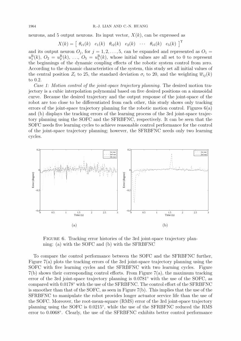
jectory is a cubic interpolation polynomial based on five desired positions on a sinusoidalcurve. Because the desired trajectory and the output response of the joint-space of therobot are too close to be differentiated from each other, this study shows only trackingerrors of the joint-space trajectory planning for the robotic motion control. Figures 6(a)and (b) displays the tracking errors of the learning process of the 3rd joint-space trajec-tory planning using the SOFC and the SFRBFNC, respectively. It can be seen that theSOFC needs five learning cycles to achieve reasonable control performance for the controlof the joint-space trajectory planning; however, the SFRBFNC needs only two learningcycles.
0 0.5 1 1.5 2 2.5 3−0.4
−0.2
0
0.2
Time (s)
Err
or (
degr
ee)
1st run3rd run5th run
(a)
0 0.5 1 1.5 2 2.5 3−0.4
−0.2
0
0.2
Time (s)
Err
or (
degr
ee)
1st run2rd run
(b)
Figure 6. Tracking error histories of the 3rd joint-space trajectory plan-ning: (a) with the SOFC and (b) with the SFRBFNC
To compare the control performance between the SOFC and the SFRBFNC further,Figure 7(a) plots the tracking errors of the 3rd joint-space trajectory planning using theSOFC with five learning cycles and the SFRBFNC with two learning cycles. Figure7(b) shows their corresponding control efforts. From Figure 7(a), the maximum trackingerror of the 3rd joint-space trajectory planning is 0.0781◦ with the use of the SOFC, ascompared with 0.0178◦ with the use of the SFRBFNC. The control effort of the SFRBFNCis smoother than that of the SOFC, as seen in Figure 7(b). This implies that the use of theSFRBFNC to manipulate the robot provides longer actuator service life than the use ofthe SOFC. Moreover, the root-mean-square (RMS) error of the 3rd joint-space trajectoryplanning using the SOFC is 0.0215◦, while the use of the SFRBFNC reduced the RMSerror to 0.0068◦. Clearly, the use of the SFRBFNC exhibits better control performance
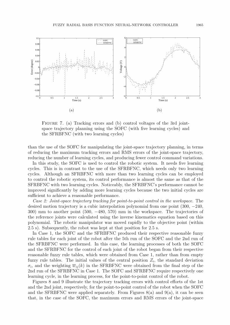
FUZZY RADIAL BASIS FUNCTION NEURAL-NETWORK CONTROLLER 1965
0 0.5 1 1.5 2 2.5 3−0.1
−0.08
−0.06
−0.04
−0.02
0
0.02
0.04
0.06
0.08
0.1
Time (s)
Err
or (
degr
ee)
SOFCSFRBFNC
(a)
0 0.5 1 1.5 2 2.5 3−6
−4
−2
0
2
4
6
Time (s)
Vol
tage
(V
)
SOFCSFRBFNC
(b)
Figure 7. (a) Tracking errors and (b) control voltages of the 3rd joint-space trajectory planning using the SOFC (with five learning cycles) andthe SFRBFNC (with two learning cycles)
than the use of the SOFC for manipulating the joint-space trajectory planning, in termsof reducing the maximum tracking errors and RMS errors of the joint-space trajectory,reducing the number of learning cycles, and producing fewer control command variations.
In this study, the SOFC is used to control the robotic system. It needs five learningcycles. This is in contrast to the use of the SFRBFNC, which needs only two learningcycles. Although an SFRBFNC with more than two learning cycles can be employedto control the robotic system, its control performance is almost the same as that of theSFRBFNC with two learning cycles. Noticeably, the SFRBFNC’s performance cannot beimproved significantly by adding more learning cycles because the two initial cycles aresufficient to achieve a reasonable performance.
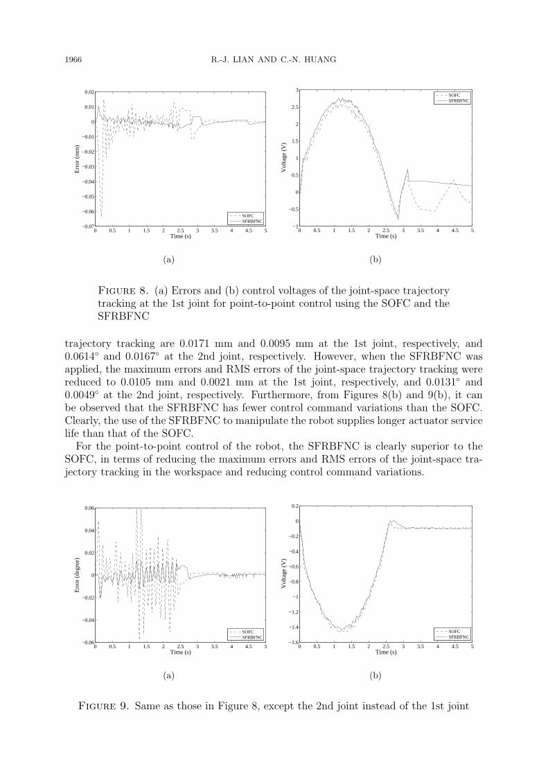
Case 2: Joint-space trajectory tracking for point-to-point control in the workspace. Thedesired motion trajectory is a cubic interpolation polynomial from one point (300, −240,300) mm to another point (500, −480, 570) mm in the workspace. The trajectories ofthe reference joints were calculated using the inverse kinematics equation based on thispolynomial. The robotic manipulator was moved rapidly to the objective point (within2.5 s). Subsequently, the robot was kept at that position for 2.5 s.
In Case 1, the SOFC and the SFRBFNC produced their respective reasonable fuzzyrule tables for each joint of the robot after the 5th run of the SOFC and the 2nd run ofthe SFRBFNC were performed. In this case, the learning processes of both the SOFCand the SFRBFNC for the control of each joint of the robot began from their respectivereasonable fuzzy rule tables, which were obtained from Case 1, rather than from emptyfuzzy rule tables. The initial values of the central position Zi, the standard deviationσi, and the weighting wij(k) in the SFRBFNC were obtained from the final step of the2nd run of the SFRBFNC in Case 1. The SOFC and SFRBFNC require respectively onelearning cycle, in the learning process, for the point-to-point control of the robot.
Figures 8 and 9 illustrate the trajectory tracking errors with control efforts of the 1stand the 2nd joint, respectively, for the point-to-point control of the robot when the SOFCand the SFRBFNC were applied separately. From Figures 8(a) and 9(a), it can be seenthat, in the case of the SOFC, the maximum errors and RMS errors of the joint-space
1966 R.-J. LIAN AND C.-N. HUANG
0 0.5 1 1.5 2 2.5 3 3.5 4 4.5 5−0.07
−0.06
−0.05
−0.04
−0.03
−0.02
−0.01
0
0.01
0.02
Time (s)
Err
or (
mm
)
SOFCSFRBFNC
(a)
0 0.5 1 1.5 2 2.5 3 3.5 4 4.5 5−1
−0.5
0
0.5
1
1.5
2
2.5
3
Time (s)
Vol
tage
(V
)
SOFCSFRBFNC
(b)
Figure 8. (a) Errors and (b) control voltages of the joint-space trajectorytracking at the 1st joint for point-to-point control using the SOFC and theSFRBFNC
trajectory tracking are 0.0171 mm and 0.0095 mm at the 1st joint, respectively, and0.0614◦ and 0.0167◦ at the 2nd joint, respectively. However, when the SFRBFNC wasapplied, the maximum errors and RMS errors of the joint-space trajectory tracking werereduced to 0.0105 mm and 0.0021 mm at the 1st joint, respectively, and 0.0131◦ and0.0049◦ at the 2nd joint, respectively. Furthermore, from Figures 8(b) and 9(b), it canbe observed that the SFRBFNC has fewer control command variations than the SOFC.Clearly, the use of the SFRBFNC to manipulate the robot supplies longer actuator servicelife than that of the SOFC.For the point-to-point control of the robot, the SFRBFNC is clearly superior to the
SOFC, in terms of reducing the maximum errors and RMS errors of the joint-space tra-jectory tracking in the workspace and reducing control command variations.
0 0.5 1 1.5 2 2.5 3 3.5 4 4.5 5−0.06
−0.04
−0.02
0
0.02
0.04
0.06
Time (s)
Err
or (
degr
ee)
SOFCSFRBFNC
(a)
0 0.5 1 1.5 2 2.5 3 3.5 4 4.5 5−1.6
−1.4
−1.2
−1
−0.8
−0.6
−0.4
−0.2
0
0.2
Time (s)
Vol
tage
(V
)
SOFCSFRBFNC
(b)
Figure 9. Same as those in Figure 8, except the 2nd joint instead of the 1st joint
FUZZY RADIAL BASIS FUNCTION NEURAL-NETWORK CONTROLLER 1967
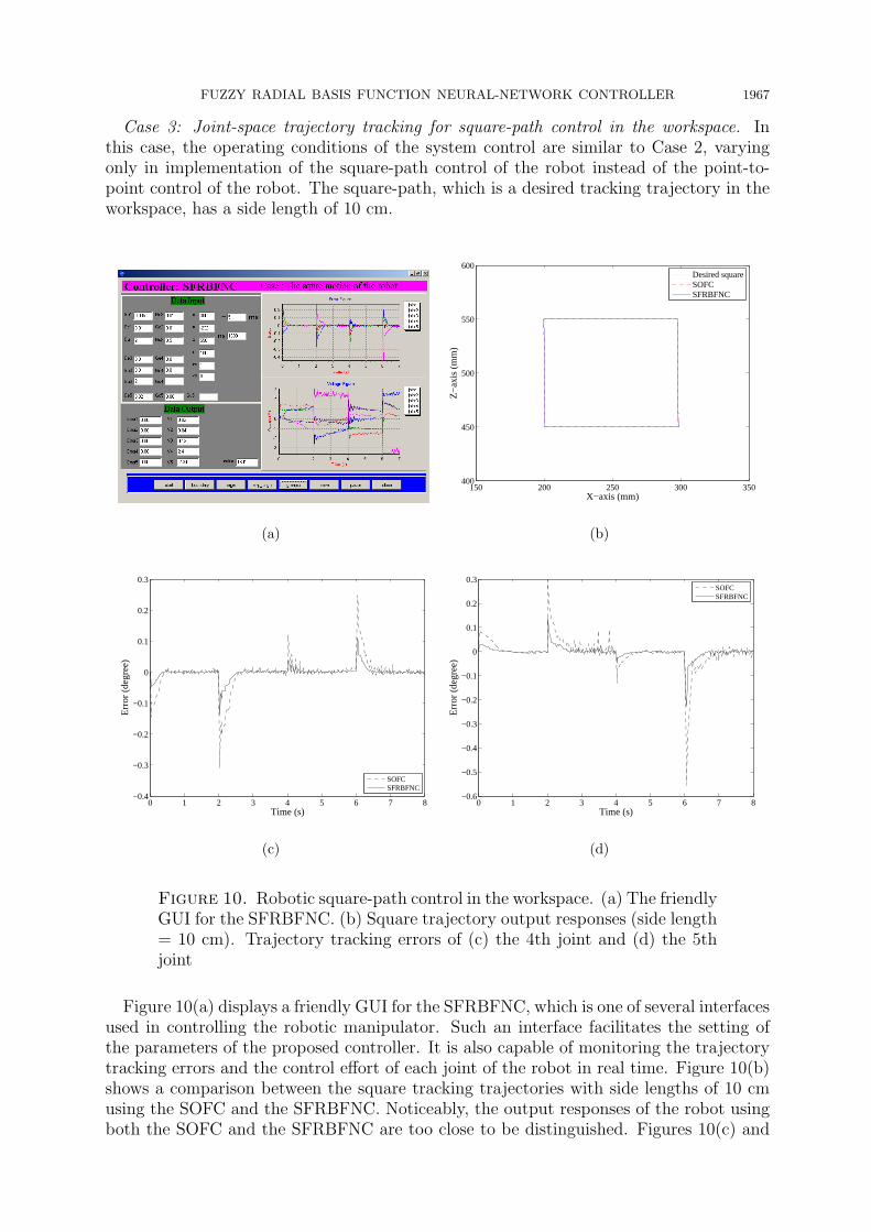
Case 3: Joint-space trajectory tracking for square-path control in the workspace. Inthis case, the operating conditions of the system control are similar to Case 2, varyingonly in implementation of the square-path control of the robot instead of the point-to-point control of the robot. The square-path, which is a desired tracking trajectory in theworkspace, has a side length of 10 cm.
(a)
150 200 250 300 350400
450
500
550
600
X−axis (mm)
Z−
axis
(m
m)
Desired squareSOFCSFRBFNC
(b)
0 1 2 3 4 5 6 7 8−0.4
−0.3
−0.2
−0.1
0
0.1
0.2
0.3
Time (s)
Err
or (
degr
ee)
SOFCSFRBFNC
(c)
0 1 2 3 4 5 6 7 8−0.6
−0.5
−0.4
−0.3
−0.2
−0.1
0
0.1
0.2
0.3
Time (s)
Err
or (
degr
ee)
SOFCSFRBFNC
(d)
Figure 10. Robotic square-path control in the workspace. (a) The friendlyGUI for the SFRBFNC. (b) Square trajectory output responses (side length= 10 cm). Trajectory tracking errors of (c) the 4th joint and (d) the 5thjoint
Figure 10(a) displays a friendly GUI for the SFRBFNC, which is one of several interfacesused in controlling the robotic manipulator. Such an interface facilitates the setting ofthe parameters of the proposed controller. It is also capable of monitoring the trajectorytracking errors and the control effort of each joint of the robot in real time. Figure 10(b)shows a comparison between the square tracking trajectories with side lengths of 10 cmusing the SOFC and the SFRBFNC. Noticeably, the output responses of the robot usingboth the SOFC and the SFRBFNC are too close to be distinguished. Figures 10(c) and
1968 R.-J. LIAN AND C.-N. HUANG
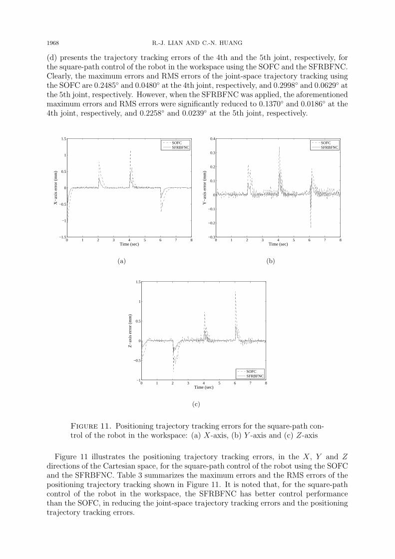
(d) presents the trajectory tracking errors of the 4th and the 5th joint, respectively, forthe square-path control of the robot in the workspace using the SOFC and the SFRBFNC.Clearly, the maximum errors and RMS errors of the joint-space trajectory tracking usingthe SOFC are 0.2485◦ and 0.0480◦ at the 4th joint, respectively, and 0.2998◦ and 0.0629◦ atthe 5th joint, respectively. However, when the SFRBFNC was applied, the aforementionedmaximum errors and RMS errors were significantly reduced to 0.1370◦ and 0.0186◦ at the4th joint, respectively, and 0.2258◦ and 0.0239◦ at the 5th joint, respectively.
0 1 2 3 4 5 6 7 8−1.5
−1
−0.5
0
0.5
1
1.5
Time (sec)
X−
axis
err
or (
mm
)
SOFCSFRBFNC
(a)
0 1 2 3 4 5 6 7 8−0.3
−0.2
−0.1
0
0.1
0.2
0.3
0.4
Time (sec)
Y−
axis
err
or (
mm
)
SOFCSFRBFNC
(b)
0 1 2 3 4 5 6 7 8−1
−0.5
0
0.5
1
1.5
Time (sec)
Z−
axis
err
or (
mm
)
SOFCSFRBFNC
(c)
Figure 11. Positioning trajectory tracking errors for the square-path con-trol of the robot in the workspace: (a) X-axis, (b) Y -axis and (c) Z-axis
Figure 11 illustrates the positioning trajectory tracking errors, in the X, Y and Zdirections of the Cartesian space, for the square-path control of the robot using the SOFCand the SFRBFNC. Table 3 summarizes the maximum errors and the RMS errors of thepositioning trajectory tracking shown in Figure 11. It is noted that, for the square-pathcontrol of the robot in the workspace, the SFRBFNC has better control performancethan the SOFC, in reducing the joint-space trajectory tracking errors and the positioningtrajectory tracking errors.
FUZZY RADIAL BASIS FUNCTION NEURAL-NETWORK CONTROLLER 1969
Table 3. Maximum errors and RMS errors of the positioning trajectorytracking for the square-path control of the robot in the workspace
SOFC SFRBFNC
Axis Max. error
(mm)
RMS error
(mm)
Max. error
(mm)
RMS error
(mm)
X 1.1508 0.2012 0.4690 0.0727
Y 0.3418 0.0525 0.1538 0.0212
Z 1.2507 0.1680 0.3665 0.0629
It can be clearly seen from the aforementioned three cases that the SFRBFNC has bettercontrol performance than the SOFC for robotic motion control. Noticeably, it is difficultto gain a perfect control performance for manipulating robotic systems when applyingthe SOFC. Therefore, to achieve the perfect performances at any operating condition, theuse of the SFRBFNC to control the robotic systems is best choice.
In addition, the RBFN, in the proposed SFRBFNC, employs the LM algorithm ratherthan the steepest descent method, which was used in the hybrid fuzzy-logic and neural-network controller (HFNC), designed by Huang and Lian [16], to minimize the objectivefunction for determining the correction value of the weighting of the RBFN. The HFNCconsists of an FLC, which was designed to control each DOF of a robot individually,and an additional coupling BP neural network, which was incorporated into an FLC tocompensate for the dynamic coupling effects between the DOFs of the robot. Although theHFNC also used a BP neural network [16] to compensate for the dynamic coupling effectsbetween the DOFs of the robot, it needed four learning cycles after training one learningcycle offline. The required data for training the BP neural network offline was obtained bythe FLC when the FLC had been used to control the robot. As mentioned previously, thedesign of the FLC has some limitations. Moreover, the convergence rate of the BP neuralnetwork with the steepest descent method is too slow to compensate for the dynamiccoupling effects between the DOFs of the robot in practical control applications. However,the LM algorithm has a faster convergence rate than the steepest descent method, so it canimprove the problem of slow convergence rates of neural networks. Although Lin and Lian[17] suggested a modified HFNC, which used the LM algorithm instead of the steepestdescent method to minimize the cost function of the BP neural network, to improve theperformance of the HFNC proposed by Huang and Lian [16], the problem of the FLCapplication still exists. Clearly, the learning capability of the SFRBFNC outperformsthose of the HFNC designed by Huang and Lian [16] and the modified HFNC designedby Lin and Lian [17] for robotic motion control. Neural networks have been adoptedin several robotic control approaches [11,12] to compensate for the effects of unknownnonlinearities, but most of their control tests were implemented in simulations instead ofactual experimentations. It is evident that the proposed SFRBFNC for robotic motioncontrol is efficient in practical applications.
5. Conclusion. This study has successfully retrofitted a 6-DOF robotic manipulator.Since the SOFC may have inappropriately chosen parameters, being able to produce anunstable system when it is applied, and the robotic control system is subject to dynamiccoupling effects between its DOFs, this study developed an SFRBFNC to eliminate oralleviate the problems faced by the practical application of the SOFC in robotic motioncontrol. Under the Windows XP operating system, the proposed controllers (SOFC andSFRBFNC) with friendly GUIs were coded using the Borland C++ Builder programminglanguage to conveniently manipulate the 6-DOF robot. Experimental results verified
1970 R.-J. LIAN AND C.-N. HUANG
that the SFRBFNC has better control performance than the SOFC for robotic motioncontrol, in terms of (1) reducing the number of learning cycles, (2) reducing the maximumtracking errors and RMS errors for the joint-space trajectory planning in the workspace,(3) decreasing the maximum errors and RMS errors of the joint-space trajectory trackingfor point-to-point control and the positioning trajectory tracking for square-path motioncontrol in the workspace, and (4) decreasing variations of the control command, therebyenhancing the actuator service life of the robotic system.
Acknowledgment. The authors would like to thank the National Science Council ofTaiwan for financially supporting this research under Contract No. NSC 100-2221-E-238-011.
REFERENCES
[1] M. K. Chang and T. H. Yuan, Experimental implementations of adaptive self-organizing fuzzy slid-ing mode control to 3-DOF rehabilitation robot, International Journal of Innovative Computing,Information and Control, vol.5, no.10(B), pp.3391-3404, 2009.
[2] M. M. Fateh and A. Azarfar, Improving fuzzy control of robot manipulators by increasing scalingfactors, ICIC Express Letters, vol.3, no.3(A), pp.513-518, 2009.
[3] G. R. Yu and L. W. Huang, Design of LMI-based fuzzy controller for robot arm using quantumevolutionary algorithms, ICIC Express Letters, vol.4, no.3(A), pp.719-724, 2010.
[4] T. J. Procyk and E. H. Mamdani, A linguistic self-organizing process controller, Automatica, vol.15,pp.15-30, 1979.
[5] S. Shao, Fuzzy self-organizing controller and its application for dynamic process, Fuzzy Sets andSystems, vol.26, pp.151-164, 1988.
[6] B. S. Zhang and J. M. Edmunds, Self-organizing fuzzy logic controller, Proc. of IEE-D ControlTheory and Applications, vol.139, no.5, pp.460-464, 1992.
[7] C. Z. Yang, Design of Real-Time Linguistic Self-organizing Fuzzy Controller, Master Thesis, Depart-ment of Mechanical Engineering, National Taiwan University, Taiwan, 1992.
[8] S. J. Huang and J. S. Lee, A stable self-organizing fuzzy controller for robotic motion control, IEEETransaction on Industrial Electronics, vol.47, no.2, pp.421-428, 2000.
[9] J. Lin and R. J. Lian, Self-organizing fuzzy controller for injection molding machines, Journal ofProcess Control, vol.20, no.5, pp.585-595, 2010.
[10] J. Lin and R. J. Lian, Self-organizing fuzzy controller for gas-injection molding combination systems,IEEE Transactions on Control Systems Technology, vol.18, no.6, pp.1413-1421, 2010.
[11] V. Kroumov, J. Yu and K. Shibayama, 3D path planning for mobile robots using simulated annealingneural network, International Journal of Innovative Computing, Information and Control, vol.6,no.7, pp.2885-2899, 2010.
[12] Y. Zuo, Y. Wang, X. Liu, S. X. Yang, L. Huang, X. Wu and Z. Wang, Neural network robust controlfor a nonholonomic mobile robot including actuator dynamics, International Journal of InnovativeComputing, Information and Control, vol.6, no.8, pp.3437-3449, 2010.
[13] R. J. Wai and C. M. Liu, Design of dynamic petri recurrent fuzzy neural network and its applicationto path-tracking control of nonholonomic mobile robot, IEEE Transactions on Industrial Electronics,vol.56, no.7, pp.2667-2683, 2009.
[14] A. Gajate, R. E. Haber, P. I. Vega and J. R. Alique, A transductive neuro-fuzzy controller: Ap-plication to a drilling process, IEEE Transactions on Neural Networks, vol.21, no.7, pp.1158-1167,2010.
[15] L. Cai, A. B. Rad and W. L. Chan, An intelligent longitudinal controller for application in semiau-tonomous vehicles, IEEE Transactions on Industrial Electronics, vol.57, no.4, pp.1487-1497, 2010.
[16] S. J. Huang and R. J. Lian, A hybrid fuzzy logic and neural network algorithm for robot motioncontrol, IEEE Transactions on Industrial Electronics, vol.44, no.3, pp.408-417, 1997.
[17] J. Lin and R. J. Lian, Hybrid fuzzy-logic and neural-network controller for MIMO systems, Mecha-tronics, vol.19, no.6, pp.972-986, 2009.
[18] S. J. Huang, K. S. Huang and K. C. Chiou, Development and application of a novel radial basisfunction sliding mode control, Mechatronics, vol.13, no.4, pp.313-329, 2003.
[19] S. Ferrari, F. Bellocchio, V. Piuri and N. A. Borghese, A hierarchical RBF online learning algorithmfor real-time 3-D scanner, IEEE Transactions on Neural Networks, vol.21, no.2, pp.275-285, 2010.
FUZZY RADIAL BASIS FUNCTION NEURAL-NETWORK CONTROLLER 1971
[20] X. Yuan, Y. Wang, W. Sun and L. Wu, RBF networks-based adaptive inverse model control systemfor electronic throttle, IEEE Transactions on Control Systems Technology, vol.18, no.3, pp.750-756,2010.
[21] F. L. Lewis, C. T. Abdallah and D. M. Dawson, Control of Robot Manipulators, Macmillan, NewYork, 1993.
[22] K. S. Fu, R. C. Gonzalez and C. S. G. Lee, Robotics Control, Sensing, Vision, and Intelligence,McGraw-Hill International Editions, 1987.
[23] V. Singh, I. Gupta and H. O. Gupta, ANN-based estimator for distillation using Levenberg-Marquardt approach, Engineering Applications of Artificial Intelligence, vol.20, no.2, pp.249-259,2007.
[24] C. Ma and C. Wang, A nonsmooth Levenberg-Marquardt method for solving semi-infinite program-ming problems, Journal of Computational and Applied Mathematics, vol.230, no.2, pp.633-642, 2009.
[25] T. P. Vogl, J. K. Mangis, A. K. Rigler, W. T. Zink and D. L. Alkon, Accelerating the convergenceof the back-propagation method, Biological Cybernetics, vol.59, no.2, pp.257-263, 1988.
[26] D. Driankov, H. Hellendoorn and M. Reinfrank, An Introduction to Fuzzy Control, Springer-Verlag,Berlin, 1993.
[27] S. J. Huang and R. J. Lian, A combination of fuzzy logic and neural network algorithms for activevibration control, Proc. of the Institution of Mechanical Engineers, Part I: Journal of Systems andControl Engineering, vol.210, no.3, pp.153-167, 1996.


![Chapter 3: Fuzzy Rules & Fuzzy Reasoning513].pdf · CH. 3: Fuzzy rules & fuzzy reasoning 1 Chapter 3: Fuzzy Rules & Fuzzy Reasoning ... Application of the extension principle to fuzzy](https://img.pdfslide.net/doc/110x75/5b3ed7b37f8b9a3a138b5aa0/chapter-3-fuzzy-rules-fuzzy-513pdf-ch-3-fuzzy-rules-fuzzy-reasoning.jpg)