SELF ORGANIZING MIGRATING ALGORITHM IN MODEL PREDICTIVE ... · 26TH DAAAM INTERNATIONAL SYMPOSIUM ON INTELLIGENT MANUFACTURING AND AUTOMATION. SELF - ORGANIZING MIGRATING ALGORITHM

26TH DAAAM INTERNATIONAL SYMPOSIUM ON INTELLIGENT MANUFACTURING AND AUTOMATION

SELF - ORGANIZING MIGRATING ALGORITHM IN MODEL

PREDICTIVE CONTROL: CASE STUDY ON SEMI-BATCH CHEMICAL REACTOR

Lubomír Macků, David Sámek

Tomas Bata University in Zlin, Faculty of Applied Informatics, nám. T.G.Masaryka 5555, 760 05 Zlín, Czech Republic

Abstract

Control of complex nonlinear systems brings challenges in the controller design. One of methods how to cope with this

challenge is the usage of advanced optimization methods. This work presents application of self-organizing migrating

algorithm (SOMA) in control of the semi-batch reactor. The reactor is used in chromium recycling process in leather

industry. Because of the complexity of this semi-batch reactor control, the model predictive control (MPC) approach is

used. The MPC controller includes self-organizing migrating algorithm (SOMA) for the optimization of the control

sequence.

KeywordsModel Predictive Control; SOMA; Chemical reactor; Exothermic reaction; Mathematical modelling

This Publication has to be referred as: Macku, L[ubomir] & Samek, D[avid] (2016). Self - Organizing Migrating

Algorithm in Model Predictive Control: Case study on Semi-Batch Chemical Reactor, Proceedings of the 26th

DAAAM International Symposium, pp.0238-0246, B. Katalinic (Ed.), Published by DAAAM International, ISBN 978-

3-902734-07-5, ISSN 1726-9679, Vienna, Austria

DOI:10.2507/26th.daaam.proceedings.033

- 0238 -


1. Introduction

In the industrial processing, there are a lot of different techniques used today. But all have a common goal - to

bring maximum profit at minimum cost. Nowadays the situation is even more complicated by the necessity of unwanted

by-products or/and products after their lifetime disposal. Of course this brings additional costs, which must be taken

into account when pricing the final product. Priority is given mainly to non-waste technologies and recycling

technologies.

One of such waste free technologies is an enzymatic dechromation. This technology recycles waste originated

during chrome tanning process and also waste generated at the end of the final product lifetime (used leather goods).

Part of the recycling process includes also an oxidation-reduction reaction which is strongly exothermic and can be

controlled by the chromium filter sludge into the hot reaction blend of chromium sulphate acid dosing [1]. Optimization

of this process control is studied in this paper.

Nomenclature

A [s-1] pre-exponential factor

cC [J·kg·K-1] specific heat capacity of the cooling water

cI [J·kg·K-1] specific heat capacity of the reaction component input

E [J·mol-1] activation energy

FI [kg.s-1] mass flow rate of the reaction component input

FC [kg.s-1] mass flow rate of the cooling water

ΔHr [J·kg-1] reaction heat

J performance criterion

K [kg·s-3·K-1] conduction coefficient

k discrete time step

mB [kg] initial mass filling of the reactor

mC [kg] weight of the cooling water in the cooling system

Nu control horizon

N1 prediction horizon beginning

N2 prediction horizon end

R [J·mol-1·K-1] gas constant

S [m2] heat transfer surface

Su control signal changes criterion function

Sy control error criterion function

T [K] reactor content temperature

TC [K] output temperature of the cooling water

TI [K] temperature of the reaction component input

TCI [K] input temperature of the cooling water

u control action (controller output)

ut tentative control signal

y system output signal

y system model response

γc speed of the γ decrement

yr desired target value of the output signal (desired response)

λ weight of the future control errors sum

ρ weight of the control action sum

2. Semi-batch chemical reactor

Process itself runs in a semi-batch chemical reactor. The chemical reactor is a vessel with a double wall filed

with a cooling medium. It has a filling opening, a discharge outlet, cooling medium openings and a stirrer. The scheme

of the reactor is depicted in the Fig. 1.

The scheme shows a reactor with initial filling mB [kg] given by the solution of chemicals without the

chromium sludge (filter cake). The sludge is fed into the reactor by FI [kg.s-1] to control the developing heat since the

temperature has to stay under a certain critical level (T(t) < 373.15K ), otherwise the reactor could be destroyed. On the

other hand it is desirable to utilize the maximum capacity of the reactor to process the maximum amount of waste in the

shortest possible time (higher temperature is desirable). Therefore an optimal control strategy has to find a trade-off

between these opposite requirements.

The feed rate is limited by the reactor walls heat transfer. The reaction is exothermic so the rising heat must be

removed. The rate of heat transfer depends on three factors [2]:

- 0239 -


Fig. 1. Semi-batch reactor scheme

1. The temperature difference between the reaction liquid and the jacket coolant. The latter depends on the coolant flow

rate, the inlet coolant temperature, and the heat-transfer rate. 2. The overall heat-transfer coefficient, which depends on

agitator mixing in the vessel and the flow rate of coolant in the jacket. 3. The heat-transfer area. If jacket cooling is

used, the effective heat-transfer area in a fed-batch reactor varies during the course of the batch directly with the volume

of liquid in the vessel.

Due to the complexity of the reaction mixture and the difficulties to perform on-line composition

measurements, control of batch and fed-batch reactors is essentially a problem of temperature control. The temperature

profile in batch reactors usually follows three-stages [3]: (i) heating of the reaction mixture until the desired reaction

temperature, (ii) maintenance of the system at this temperature and (iii) cooling stage in order to minimize the formation

of by-products. Any controller used for the reactor control must be able to overcome these different stages.

3. Mathematical model

The above mentioned reactor can be described by the mathematical model shown below. Under usual simplifications,

based on the mass and heat balance, the following 4 nonlinear ordinary differential equations can be derived [4]:

IF

t

tm

d

d (1)

taeAtm

taF

t

ta tTR

E

I

)](1[

d

d (2)

tm

FtT

ctm

tTSK

ctm

tTSK

c

taHeA

ctm

TcF

t

tT ICrtTR

E

III

d

d

(3)

C

CC

CC

C

CCC

CICC

m

tTF

cm

tTSK

cm

tTSK

m

TF

t

tT

d

d (4)

Individual symbols have the following meaning: m is the total weight of reaction components in the reactor, a

is the mass concentration of the reaction component in the reactor, c = 4500 J·kg·K-1 is the specific heat capacity of the

reactor content and T its temperature. FI, TI = 293.15 K and cI = 4400 J·kg·K-1 is the reaction component input mass

flow rate, temperature and specific heat capacity. FC = 1 kg·s-1, TCI = 288.15 K, TC, cC = 4118 J·kg·K-1 and mC = 220 kg

is the cooling water mass flow rate, input temperature, output temperature, specific heat capacity and weight of the

cooling water in the cooling system of the reactor, respectively. Other constants: A = 219.588 s-1, E = 29967.5087 J·mol-

1, R = 8.314 J·mol-1·K-1, ΔHr = 1392350 J·kg-1, K = 200 kg·s-3·K-1, S = 7.36 m2.

The fed-batch reactor use jacket cooling, but the effective heat-transfer area (S = 7.36 m2) in the mathematical

model was treated as constant, not time varying. The initial amount of material placed in the reactor takes about two-

thirds of the in-reactor volume and the reactor is treated as ideally stirred, so we can do this simplification.

Variables FI, FC, TI, TCI, can serve as manipulated signals. However, from practical point of view, only FI and FC are

usable. The TI or TCI temperature change is inconvenient due to the economic reasons (great energy demands).3.1.

F , T , cI I I

F , T , cC CI CF , T , cC C C

m , T , cC C C

m, m , a, T, cB

- 0240 -


3.1 Technological limits and variables saturation

Maximum filling of the reactor is limited by its volume to m = 2450kg approximately. The process of the

chromium sludge feeding FI has to be stopped by this value. Practically, the feeding FI can vary in the range 3;0IF

kg.s-1. As stated in the system description, the temperature T(t) must not exceed the limit 373.15K ; this temperature

value holds also for the coolant (water) but it is not so critical in this case as shown by the further experiments.

4. SOMA algorithm

The Self-Organizing Migrating Algorithm is used for the above mentioned system optimization. SOMA

algorithm can be used for optimizing any problem which can be described by an objective function. This algorithm

optimizes a problem by iteratively trying to improve a candidate solution, i.e. a possible solution to the given problem.

The SOMA has been successfully utilized in many applications [5-7], while interesting comparison to with simulated

annealing and differential evolution is provided by Nolle et al. in [8].

SOMA is based on the self-organizing behavior of groups of individuals in a “social environment”. It can be

classified in two ways – as an evolutionary algorithm or as a so-called memetic algorithm. During a SOMA run,

migration loops are performed causing individuals repositioning as in evolutionary algorithm. The position of the

individuals in the search space is changed during a generation, called a ‘migration loop’. Individuals are generated by

random according to what is called the ‘specimen of the individual’ principle. The specimen is in a vector, which

comprises an exact definition of all those parameters that together lead to the creation of such individuals, including the

appropriate constraints of the given parameters. [9]. On the other hand, no new ‘children’ are created in the common

‘evolutionary’ way. The category of memetic algorithms covers a wide class of meta-heuristic algorithms. We can say

that memetic algorithms are classified as competitive-cooperative strategies showing synergetic attributes. [10]. SOMA

shows these attributes as well. Because of this, it is more appropriate to classify SOMA as a memetic algorithm.

5. Control of the reactor

Despite the fact that various reactors have been widely used in the chemical industry for decades, the efficient

reactor control still encounters many difficulties. There have been published a lot of works dealing with the reactor

control approaches. Good introduction to chemical reactors provides for example [11] or [12]. The state of art of

chemical reactors control presents Luyben in [13] and [14], control and monitoring of batch reactors describes

Caccavale et al. in [15]. Generally, it can be stated that chemical reactors controllers uses various control methods, such

as PI controllers, adaptive control methods, robust approaches, predictive control and the like [16-25]. The model

predictive control [26-28] belongs to the one of the most popular and successful approaches for semi-batch reactors

control. However, this methodology brings some difficulties in finding optimal control sequence especially when

complex nonlinear model is utilized. Interesting way how to cope with the optimization problem offers the usage of

evolutionary algorithms [29], [30].

In this paper two different approaches to the model predictive control of the given plant are introduced. At first, the

model predictive controller that uses self-organizing migrating algorithm for the optimization of the control sequence is

presented. This methodology ensues from model predictive control method [3] while it uses same value of the control

signal for whole control horizon. This modification was applied in order to reduce computational demands of the

controller. The classic MPC controller, which uses Matlab Optimization Toolbox for obtaining the optimal control

sequence, is used as the comparative method. This MPC controller computes the control sequence at every sampling

period but only first value is applied.

5.1. Notation

From the systems theory point of view the reactor manipulated variables here are input flow rates of the

chromium sludge FI and of the coolant FC. Input temperatures of the filter cake TI and of the coolant TCI can be

alternatively seen as disturbances. Although the system is generally MIMO, it is assumed just as a single input – single

output (SISO) system in this chapter. Thus, the only input variable is the chromium sludge flow rate FI and the coolant

flow rate FC is treated as a constant. This input variable, often called control action, is in the control theory denoted as

u. The output signal to be controlled is again the temperature inside the reactor T. The output signal is usually in the

control theory denoted as y and consequently the desired target value of the output signal as yr.

5.2. Model predictive control

The main idea of MPC algorithms is to use a dynamical model of process to predict the effect of future control actions

on the output of the process. Hence, the controller calculates the control input that will optimize the performance

criterion J over a specified future time horizon [31]:

- 0241 -


uN

i

tt

N

Ni

r ikuikuikyikykJ

1

2221ˆ

2

1

(5)

where k is discrete time step, N1, N2 and Nu define horizons over which the tracking error and the control increments are

evaluated. The ut variable is the tentative control signal, yr is the desired response and y is the network model

response. The parameters λ and ρ determine the contribution that the sums of the squares of the future control errors and

control increments have on the performance index.

Typically, the receding horizon principle is implemented, which means that after the computation of optimal

control sequence only the first control action is implemented. Then, the horizon is shifted forward one sampling instant

and the optimization is again restarted with new information from measurements. Simplified structure of the MPC

control strategy is depicted in the figure 2.

5.3. Model predictive control using SOMA

All simulations with algorithm SOMA were performed in the Mathematica 8.0 software. Here the algorithm

SOMA was used for the cost function (5) minimization and was set as follows: Migrations = 25; AcceptedError = 0.1;

NP = 20; Mass = 3; Step = 0.3; PRT = 0.1; Specimen = {0.0, 3.0, 0.0}; Algorithm strategy was chosen All To One. First

two parameters serve for the algorithm ending. Parameter “Migrations” determines the number of migration loops,

“AcceptedError” is the difference between the best and the worst individuals (algorithm accuracy). If the loops exceed

the number set in “Migrations” or “AcceptedError” is larger than the difference between the best and the worst

individuals, the algorithm stops. Other parameters influence the quality of the algorithm running. “NP” is the number of

individuals in the population (its higher value implicates higher demands on computer hardware and can be set by user),

“Mass” is the individual distance from the start point, “Step” is the step which uses the individual during the algorithm,

“PRT” is a perturbation which is similar to hybridizing constant known from genetic algorithms or differential

evolutions. “Specimen” is the definition of an exemplary individual for whole population. For details see [9].

Fig. 2. Basic structure of the model predictive controller

There were performed seven different simulations using SOMA algorithm described in this section. First tree

simulations (SOMA1 – SOMA3) were done to study the control horizon Nu influence, next three (SOMA4 – SOMA6)

the prediction horizon N2 influence and the last one (SOMA7) is the simulation with an optimal setting. All settings can

be seen in Table 1.

λ ρ N2 Nu

SOMA1 1 1 300 30

SOMA2 1 1 300 60

SOMA3 1 1 300 90

SOMA4 1 1 200 60

SOMA5 1 1 280 60

SOMA6 1 1 360 60

SOMA7 1 1 320 60

Table 1. SOMA controller settings

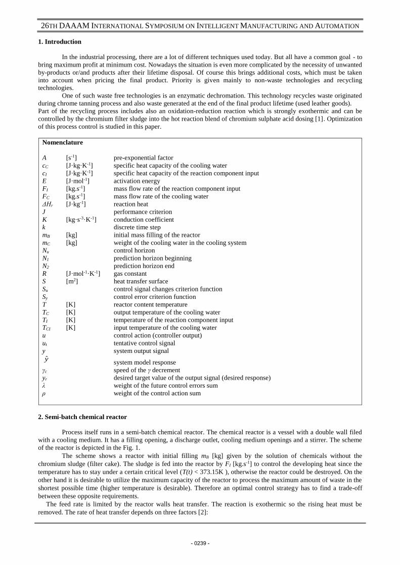
Graphical output of SOMA7 (the optimal settings) simulation is depicted in figure 3. Only two most important

dependencies are shown – the in-reactor temperature and the chromium sludge dosing development. As was already

PLANT

MODELOPTIMIZATION

y

y

u

CONTROLLER reference trajectory

predicted outputspredicted control errors e

constraintscostfunction

ut

- 0242 -


said, the temperature has to stay under critical point 373.15K. The chromium sludge dosing shouldn’t embody any rapid

changes.

The control horizon (Nu) actually means the time interval, for which the actuating variable (FI) has constant

value. It is generally better to set it as short as possible because of more rapid influence on the system, but on the other

hand it increases the computing time during the calculations. So it is necessary to find the control horizon value, which

balance between these two requirements.

The prediction horizon (N2) determines how forward controller knows the system behavior. If the horizon is

too short, the controller doesn’t react in time and the system may become uncontrollable. Long horizon means again the

more demanding computation, i.e. the need of more powerful computer hardware.

Fig. 3. Results of SOMA7 simulations

5.4. Conventional model predictive approach

The comparative method is based on the classical MPC strategy described in the part 5.2. The optimization box

(see figure 2) utilizes standard Matlab Optimization Toolbox function fmincon and receding control strategy was

implemented. The fmincon function used trust-region-reflective algorithm [32].

For the reason that the compared controllers SOMA applied the same control action for whole length of the

control horizon Nu= 60 (with the sample time = 1s), the sample time of the comparative controllers was set to 60s. The

control horizon Nu was set to 10 as well as the prediction horizon N2. The rest of the controller design remained same –

the predictor was based on the white-box model described by equations (1 – 4), cost function of MPC was the

same.

The control loop was simulated using Matlab/Simulink, the controller was built-in as the Matlab M-File and

predictor used Matlab S-Function technology.

λ ρ γ γc N1 N2 Nu

MPC1 1 100 0 0 1 10 10

MPC2 1 100 2000 100 1 10 10

MPC3 1 100 2000 200 1 10 10

MPC4 1 100 1500 100 1 10 10

Table 2. Settings of the controllers

However, such controller (Table 2 MPC1 settings) that follows equation (5), did not provide acceptable results. It was

not possible to avoid either the overshoot of the in-reactor temperature or the permanent control error using the control

configuration. It results from simulations that the biggest problem comes in the very beginning of the control, when the

control error is the highest and the controller performs enormous control actions. This is caused by the fact that the

reaction is strongly exothermic and even small concentration of the filter cake causes steep rise of the temperature.

- 0243 -


Thus, the enhancement of the criterion (5) that penalizes values of the control signal in the beginning of semi-batch

process was necessary. Also, at the same time the penalization has to decrease taperingly (6-7):

uu N

i

t

N

i

tt

N

Ni

r ikukikuikuikyikykJ

11

2221ˆ

2

1

(6)

ckk (7)

where γc is the parameter which defines the speed of the decrement in γ. This enhancement brought possibility to

influence more intensely the speed of dosing of the filter cake with two parameters. In other words γ parameter defines

the level of penalization of the control signal, while the ratio γ/γc specifies the length of the penalization interval.

However, too high γ parameter or γ/γc ratio caused unavailing delays or oscillations (the settings MPC2 in Table 2). On

the other hand, small γ/γc ratio led to overshoots of the temperature (the settings MPC3 in Table 2). The best result

which was obtained using this approach was obtained for MPC4 settings and is presented in figure 4.

Fig. 4. Control of the semi-batch reactor using MPC4 controller

6. Comparison

The best representatives of the two different approaches were selected to be compared in this section. In order

to describe the control error the criterion function Sy was defined:

ft

i

ry iyiyS

1

2 (8)

T he criterion Su describes the speed of the control signal changes. Monitoring of it is very important, because

lifetime of the mud pump that injects the filter cake solution to the reactor would be significantly shortened due to steep

changes of delivery.

ft

i

u iuiuS

1

21 (9)

The tf defines number of steps for that are the criterions Sy and Su computed. In this paper the tf was set to 50

steps, because only the first 3000 seconds provide information about control. The dosing (control) commonly finishes

shortly after 3000s and after that only cooling is performed.

0 500 1000 1500 2000 2500 3000300

320

340

360

380

400

time [s]

T [

K]

reference signal

system output

0 500 1000 1500 2000 2500 30000

0.5

1

1.5

2

2.5

3

time [s]

FI

[kg/s

]

- 0244 -


For the reason that the plant is very exothermic and it is very sensitive to the exceeding of the desired value of

the temperature (yr = 370K), it was necessary to observe the maximum overshoot of the output value ymax. Furthermore,

it is essential to observe the time of the reaction (dosing) tb.

As can be seen from Table 3, the in-reactor temperature overshoots were in both cases quite similar.

Nevertheless, the overshoot obtained by using SOMA algorithm is a little bit lower. As far as the criterion Sy, we need

as low value as possible - the lower value the better. Even if the results were again close, the SOMA provided the lower

value, which means that quality of the control was better too. The time of dosing achieved by SOMA was shorter

approximately for one minute (58 seconds).

The only criterion which was better in MPC control was the Su. Here the value 2.3200 is quite higher than

1.5500. For the actuating device it means higher loading and shorter lifetime.

controller

Sy

K2

Su

kg2·s-2

ymax

K

tb

s

SOMA7 9.2571·103 2.3200 370.1740 3242

MPC4 1.0333·104 1.5500 370.2358 3300

Table 3. Comparison of the controllers

7. Conclusion

The paper presented comparison of two approaches to semi-batch process model predictive control. Firstly, the

Self Organizing Migrating Algorithm implemented in Mathematica software was used for cost function optimization.

Secondly, as the comparative method model predictive controller implemented in Matlab was selected. This controller

used built-in function fmincon from Matlab Optimization Toolbox instead of SOMA. It can be concluded that both

algorithms provided applicable results. Nevertheless, SOMA provided slightly faster semi-batch process. What is more,

the comparative method based on Matlab Optimization Toolbox required modification of the cost function in order to

obtain appropriate control.

The comparison itself was made from four points of view. Firstly, the value of the in-reactor temperature overshoot and

the related quality of the in-reactor temperature course were observed. Secondly, the time of processing which is

important for effectiveness of a real plant and also the course of the actuating signal that is important from the practical

point of view were monitored.

The paper showed that Self Organizing Migrating Algorithm successfully improved the control performance of the

selected plant. It can be concluded that evolutionary algorithms should be considered as good way how to optimize

control sequence in model predictive control, especially in case of complex nonlinear systems.

8. References

[1] K. Kolomaznik, M. Adamek and M.Uhlirova, “Potential Danger of Chromium Tanned Wastes,” in HTE'07:

Proceedings of the 5th IASME / WSEAS International Conference on Heat Transfer, Thermal Engineer-ing and

Environment, pp. 136-140, WSEAS, Athens, Greece, 2007.

[2] W. L. Luyben, “Fed-Batch Reactor Temperature Control Using Lag Compensation and Gain Scheduling,” Ind &

Eng Chem Res, vol. 43, no. 15, pp. 4243-4252, 2004.

[3] H. Bouhenchir, M. Cabassud and M. V. Le Lann, “Predictive functional control for the temperature control of a

chemical batch reactor,” Comp and Chem Eng, vol. 30, no. 6-7, pp. 1141-1154, 2006.

[4] F. Gazdos and L. Macku, “Analysis of a semi-batch reactor for control purposes,” in Proceedings of 22nd

European Conference on Modelling and Simulation ECMS 2008, pp. 512-518, ECMS, Nicosia, Cyprus, 2008.

[5] L. S. Coelho and V. C. Marianib, “An efficient cultural self-organizing migrating strategy for economic dispatch

optimization with valve-point effect,” Energy Conversion and Management, vol. 51, no. 12, pp. 2580-2587, 2010.

[6] K. Deep and Dipti, “A self-organizing migrating genetic algorithm for constrained optimization,” Applied

Mathematics and Computation, vol. 198, no. 1, pp. 237-250, 2008.

[7] Singh, D., & Agrawal, S., Log-logistic SOMA with quadratic approximation crossover. Paper presented at the

International Conference on Computing, Communication and Automation, ICCCA 2015, 146-151, 2015.

[8] L. Nolle, I. Zelinka, A.A. Hopgood and A. Goodyear, “Comparison of an self-organizing migration algorithm with

simulated annealing and differential evolution for automated waveform tuning,” vol. 36, no. 10, pp. 645-653,

2005.

[9] I. Zelinka, “SOMA - Self Organizing Migrating Algorithm,” in G. Onwubolu and B. V. Babu (eds) New

Optimization Techniques in Engi-neering, pp. 167-217. Springer-Verlag, London, UK, 2004.

[10] J. Lampinen and I. Zelinka, “Mechanical engineering design optimization by differential evolution,” in: D. Corne,

M. Dorigo, Glover (Eds.), New Ideas in Optimization. McGraw Hill, London, UK, pp. 127-146, 1999.

[11] E. B. Nauman, Chemical Reactor Design, Optimization, and Scaleup, McGraw-Hill, New York, 2002.

- 0245 -


[12] U. Mann, Principles of Chemical Reactor Analysis and Design - New Tools for Industrial Chemical Reactor

Operations, John Wiley & Sons, Hoboken, NJ, 2009.

[13] W. L. Luyben, Chemical Reactor Design and Control, John Wiley & Sons, Hoboken, NJ, 2007.

[14] W. L. Luyben, Process Modeling, Simulation and Control for Chemical Engineers, McGraw-Hill, New York,

1996.

[15] F. Caccavale, M. Iamarino, F. Pierri and V. Tufano, Control and Monitoring of Chemical Batch Reactors, Springer

– Verlag, London, 2011.

[16] E. Aguilar-Garnica, J. P. Garcia-Sandoval and V. Gonzalez-Alvarez, “PI controller design for a class of distributed

parameter systems,” Chemical Engineering Science, vol. 66, no. 15, pp. 4009–4019, 2001.

[17] R. Aguilar-Lopez, R. Martinez-Guerra and R. Maya-Yescas, “Temperature Regulation via PI High-Order Sliding-

Mode Controller Design: Application to a Class of Chemical Reactor,” International Journal of Chemical Reactor

Engineering, vol. 7, no. 1, 2009.

[18] J. Vojtesek and P. Dostal, “Simulation of Adaptive Control Applied on Tubular Chemical Reactor,” WSEAS

Transactions on Heat and Mass Transfer, vol. 6, no. 1, pp. 1-10, 2011.

[19] J. Vojtesek and P. Dostal, “Two Types of External Linear Models Used for Adaptive Control of Continuous

Stirred Tank Reactor,” in Proceedings of the 25th European Conference on Modelling and Simulation, pp. 501-

507, ECMS, Krakow, Poland, 2011.

[20] A. Leosirikul, D. Chilin, J. Liu, J. F. Davis and P. D. Christofides, “Monitoring and retuning of low-level PID

control loops,” Chemical Engineering Science, vol. 69, no. 1, pp. 287-295, 2012.

[21] W. Du, X. Wu and Q. Zhu, “Direct design of a U-model-based generalized predictive controller for a class of

nonlinear (polynomial) dynamic plants,” Proceedings of the Institution of Mechanical Engineers, Part I: Journal of

Systems and Control Engineering, vol. 226, no. 1, pp. 27-42, 2012.

[22] R. Zhang, A. Xue and S. Wang, “Dynamic Modeling and Nonlinear Predictive Control Based on Partitioned

Model and Nonlinear Optimization,” Industrial & Engineering Chemistry Research, vol. 50, no. 13, pp. 8110-

8121, 2011.

[23] R. Matusu, J. Zavacka, R. Prokop and M. Bakosova, “The Kronecker SummationMethod for Robust Stabilization

Applied to a Chemical Reactor,” Journal of Control Science and Engineering, vol. 2011, article ID 273469, 2011.

[24] M. A. Hosen, M. A. Hussain and F. S. Mjalli, “Control of polystyrene batch reactors using neural network based

model predictive control (NNMPC): An experimental investigation,” Control Engineering Practice, vol. 19, no. 5,

pp. 454–467, 2011.

[25] K. Y. Rani and S. C. Patwardhan, “Data-Driven Model Based Control of a Multi-Product Semi-Batch

Polymerization Reactor,” Chemical Engineering Research and Design, vol. 85, no. 10, 2007.

[26] F. Xaumiera, M. V. Le Lann, M. Cabassud and G. Casamatta, “Experimental application of nonlinear model

predictive control: temperature control of an industrial semi-batch pilot-plant reactor,” Journal of Process Control,

doi: 10.1016/S0959-1524(01)00057-9, 2002.

[27] N. Hvala, F. Aller, T. Miteva and D. Kukanja, “Modelling, simulation and control of an industrial, semi-batch,

emulsion-polymerization reactor,” Computers and Chemical Engineering, vol. 35, no. 10, pp. 2066– 2080, 2011.

[28] J. Oravec, M. Bakošová, “Robust model-based predictive control of exothermic chemical reactor”, Chemical

Papers, 69 (10), pp. 1389-1394, 2015.

[29] T. T. Dao, “Investigation on Evolutionary Computation Techniques of a Nonlinear System”, Modelling and

Simulation in Engineering, vol. 2011, Article ID 496732, 2011.

[30] I. Zelinka, D. Davendra, R. Šenkeřík, M. Pluháček, “Investigation on evolutionary predictive control of chemical

reactor” Journal of Applied Logic, 13 (2), pp. 156-166, 2015.

[31] E. F. Camacho and C. Bordons, Model Predictive Control in the Process Industry. Springer - Verlag, London,

2004.

[32] T. F. Coleman and Y. Zhang, Fmincon [online]. Mathworks, Natick.

http://www.mathworks.com/help/toolbox/optim/ug/fmincon.html. Ac-cessed 25 September 2011.

- 0246 -

Documents

SELF ORGANIZING MIGRATING ALGORITHM IN MODEL PREDICTIVE ... · 26TH DAAAM INTERNATIONAL SYMPOSIUM ON INTELLIGENT MANUFACTURING AND AUTOMATION. SELF - ORGANIZING MIGRATING ALGORITHM