Self-Similar Solutions of Three-Dimensional Navier—Stokes Equation

This article has been downloaded from IOPscience. Please scroll down to see the full text article.

2011 Commun. Theor. Phys. 56 745

(http://iopscience.iop.org/0253-6102/56/4/25)

Download details:

IP Address: 148.6.96.235

The article was downloaded on 21/10/2011 at 12:43

Please note that terms and conditions apply.

View the table of contents for this issue, or go to the journal homepage for more

Home Search Collections Journals About Contact us My IOPscience

Commun. Theor. Phys. 56 (2011) 745–750 Vol. 56, No. 4, October 15, 2011

Self-Similar Solutions of Three-Dimensional Navier–Stokes Equation

I.F. Barna∗

KFKI Atomic Energy Research Institute of the Hungarian Academy of Sciences, Thermohydraulics Department, (KFKI-AEKI), H-1525 Budapest, P.O. Box 49, Hungary

(Received March 15, 2011; revised manuscript received June 22, 2011)

Abstract In this article we will present pure three dimensional analytic solutions for the Navier–Stokes and the

continuity equations in Cartesian coordinates. The key idea is the three-dimensional generalization of the well-known

self-similar Ansatz of Barenblatt. A geometrical interpretation of the Ansatz is given also. The results are the Kum-

mer functions or strongly related. Our final formula is compared with other results obtained from group theoretical

approaches.

PACS numbers: 47.10.adKey words: Navier–Stokes equation, self-similar solution

To describe the dynamics of viscous incompressible flu-ids the Navier–Stokes (NS) partial differential equation(PDE) together with the continuity equation have to beinvestigated. In Cartesian coordinates and Eulerian de-scription these equations have the following form:

∇v = 0, vt + (v∇)v = ν△v − ∇pρ

+ a , (1)

where v, ρ, p, ν, a denote respectively the three-dimensional velocity field, density, pressure, kinematic vis-cosity, and an external force (like gravitation) of the in-vestigated fluid (To avoid further misunderstanding weuse a for external field instead of the letter g, whichis reserved for a self-similar solution). In the follow-ing ν, a are parameters of the flow. For a better trans-parency in the following we use the coordinate notationv(x, y, z, t) = u(x, y, z, t), v(x, y, z, t), w(x, y, z, t) and forthe scalar pressure variable p(x, y, z, t)

ux + vy + wz = 0 ,

ut + uux + vuy + wuz

= ν(uxx + uyy + uzz) −px

ρ,

vt + uvx + vvy + wvz

= ν(vxx + vyy + vzz) −py

ρ,

wt + uwx + vwy + wwz

= ν(wxx + wyy + wzz) −pz

ρ+ a . (2)

The subscripts mean partial derivations. According toour best knowledge there are no analytic solutions forthe most general three-dimensional case. However, thereare various examination techniques available in the lit-erature. Manwai[1] studied the N -dimensional (N ≥ 1)radial Navier–Stokes equation with different kind of vis-cosity and pressure dependences and presented analyticalblow up solutions. His works are still (1+1)-dimensional

(one spatial and one time dimension) investigations. An-other well established and popular investigation methodis based on Lie algebra there are numerous studies avail-able. Some of them are even for the three-dimensionalcase, for more see [2]. Unfortunately, no explicit solutionsare shown and analyzed there. Fushchich et al.

[3] con-structed a complete set of G(1, 3)-inequivalent Ansatze ofcodimension 1 for the NS system, they present 19 differ-ent analytical solutions for one or two space dimensions.Their last solution is very closed to ours one but not iden-tical, we will come back to these results later. Further two-and three-dimensional studies based on group analyticalmethod were presented by Grassi et al.[4] They also pre-sented solutions, which look almost the same as ours, butthey considered only 2 space dimensions. We will comparethese results to ours one at the end of the paper.

Recently, Hu et al.[5] presented a study where sym-

metry reductions and exact solutions of the (2+1)-dimensional NS were presented. Aristov and Polyanin[6]

used various methods like Crocco transformation, gener-alized separation of variables or the method of functionalseparation of variables for the NS and presented largenumber of new classes of exact solutions. Sedov in hisclassical work[7] presented analytic solutions for the tree-dimensional spherical NS equation where all three velocitycomponents and the pressure have polar angle dependence(θ) only. Even this kind of restricted symmetry led to anon-linear coupled ordinary differential equation systemwhich a very rich mathematical structure. Some similarityreduction solutions of the two-dimensional incompressibleNS equation was presented by [8]. Additional solutions areavilable for the (2+1)-dimensional NS also via symmetryreduction techniques by [9].

Beyond the NS system there are other important andpopular PDEs, which attract much interest and investiga-tion. The applied methods are the same there, too. With-out completeness we mention some examples. For one-

∗E-mail: barnai@aeki.kfki.hu

c© 2011 Chinese Physical Society and IOP Publishing Ltd

http://www.iop.org/EJ/journal/ctp http://ctp.itp.ac.cn

746 Communications in Theoretical Physics Vol. 56

dimensional cubic-quintic nonlinear Schrodinger equationa quite general self-similar type of solution ψ(z, t) =u(z, t) exp[iv(z, t)] was applied where u and v are realfunctions.[10] The results are analytic solutions for an ex-ternal potential with variable coefficients. A more generaltype of this Ansatz u(z, t) = A(z)U [T (z, t)] exp(iϕ(z, t))was used with success to get chirped and chirp-free self-similar conoidal solitary wave solutions[11] for the sameequation. Such solutions can be generalized for multi-dimensional spatial coordinates. There are analytic soli-tary wave solutions available for the (3+1)-dimensionalGross–Pitaevskii equation with the following Ansatz ψ =u(x, y, z, t)R(t) exp[ib(t)(x2 + y2 + z2)].[12]

Fig. 1 A self-similar solution of Eq. (3) for t1 < t2. Thepresented curves are Gaussians for regular heat conduc-tion.

From basic textbooks the form of the one-dimensionalself-similar Ansatz is well-known[7,13−14]

T (x, t) = t−αf( x

tβ

)

: = t−αf(η) , (3)

where T (x, t) can be an arbitrary variable of a PDE andt means time and x means spatial dependence. The sim-ilarity exponents α and β are of primary physical impor-tance since α represents the rate of decay of the magni-tude T (x, t), while β is the rate of spread (or contractionif β < 0) of the space distribution as time goes on. Themost powerful result of this Ansatz is the fundamental orGaussian solution of the Fourier heat conduction equa-tion (or for Fick’s diffusion equation) with α = β = 1/2.These solutions are visualized on Fig. 1, for time pointst1 < t2. In the pioneering work of Leray[15] in 1934 atthe end of the manuscript he asks whether it is possi-ble to construct self-similar solutions to the NS systemin R

3 in the form of p(x, t) = [1/(T − 1)]P (x/√T − t)

and v(x, t) = (1/√T − t)V (x/

√T − t). In 2001 Miller

et al.[16] proved the nonexistence of singular pseudo-self-

similar solutions of the NS system with such kind of solu-tions. Unfortunately, there is no direct analytic calcula-tion with the 3-dimensional self-similar generalization ofthis Ansatz in the literature. We will show later on thatin our case the time dependence has the same exponentsas showed above.

Applicability of this Ansatz is quite wide and comesup in various transport systems.[7,13−14,17−19] This Ansatzcan be generalized for two or three dimensions in variousways one is the following

u(x, y, z, t) = t−αf(F (x, y, z)

tβ

)

: = t−αf(x+ y + z

tβ

)

:

= t−αf(ω) , (4)

where F (x, y, z) can be understood as an implicit param-eterization of a two-dimensional surface. If the functionF (x, y, z) = x + y + z = 0, which is presented on Fig. 2,then it is an implicit form of a plane in three dimensions.At this point we can give a geometrical interpretation ofthe Ansatz. Note that the dimension of F (x, y, z) still hasto be a spatial coordinate. With this Ansatz we considerall the x coordinate of the velocity field vx = u where thesum of the spatial coordinates are on a plane on the samefooting. We are not considering all the R3 velocity fieldbut a plane of the vx coordinates as an independent vari-able. The Navier–Stokes equation - which is responsiblefor the dynamics - maps this kind of velocities, which areon a surface to another geometry. In this sense we caninvestigate the dynamical properties of the NS equationtruly.

Fig. 2 The graph of the x + y + z = 0 plane.

In principle there are more possible generalization ofthe Ansatz available. One is the following:

u(x, y, z, t) = t−αf(

√

x2 + y2 + z2 − a

tβ

)

:

= t−αf(ω) , (5)

which can be interpreted as an Euclidean vector norm orL2 norm. Now we contract all the x coordinate of thevelocity field u (which are on a surface of a sphere withradius a) to a simple spatial coordinate. Unfortunately,if we consider the first and second spatial derivatives andplug them into the Navier–Stokes equation we cannot geta pure η dependent ordinary differential equation (ODE)system some explicit x, y, z or t dependence tenaciouslyremain. For a telegraph-type heat conduction equation

No. 4 Communications in Theoretical Physics 747

both these Ansatzes are useful to get solutions for thetwo-dimensional case.[19]

Now we concentrate on the first Ansatz (4) and searchthe solution of the Navier–Stokes PDE system in the fol-lowing form:

u(x, y, z, t) = t−αf(x+ y + z

tβ

)

,

v(x, y, z, t) = t−γg(x+ y + z

tδ

)

,

w(x, y, z, t) = t−ǫh(x+ y + z

tζ

)

,

p(x, y, z, t) = t−ηl(x+ y + z

tθ

)

, (6)

where all the exponents α, β, γ, δ, ǫ, ζ, η, θ are real numbers(Solutions with integer exponents are called self-similarsolutions of the first kind, non-integer exponents meanself-similar solutions of the second kind). The functionsf, g, h, l are arbitrary and will be evaluated later on. Ac-

cording to Eq. (2) we need to calculate all the first timederivatives of the velocity field, all the first and second spa-tial derivatives of the velocity fields and the first spatialderivatives of the pressure. All these derivatives are notpresented in details. Note that both Eq. (2) and Eq. (8)have a large degree of exchange symmetry in the coordi-nates x, y, and z. Later we want to have an ODE systemfor all the four functions f(ω), g(ω), h(ω), l(ω) which allhave to have the same argument ω. This dictates theconstraint that β = δ = ζ = θ have to be the samereal number, which reduces the number of free parame-ters (let us use the β from now on ω = (x+ y + z)/tβ).From this constrain follows that e.q. ux = f ′(ω)/tα+β ≈vy = f ′(ω)/tγ+β where prime means derivation with re-spect to ω. This example shows the hidden symmetry ofthis construction, which may help us. For the better un-derstanding we present the second equation of (2) afterthe substitution of the Ansatz (9).

− αt−α−1f(ω) − βt−α−1f ′(ω)ω + t−2α−βf(ω)f ′(ω) + t−γ−α−βg(ω)f ′(ω) + t−ǫ−α−βh(ω)f ′(ω)

= ν3t−α−2βf ′′(ω) − t−µ−βl′(ω)

ρ. (7)

To have an ODE which only depends on ω (which is now the new variable instead of time t and the radialcomponents) all the time dependences e.g. t−α−1 have to be zero or all the exponents have to be the same. After somealgebra it comes out that all the six exponents α− ζ included for the velocity filed (the first three functions in Eq. (8))have to be +1/2. The only exception is the term with the gradient of the pressure. There η = 1 and θ = 1/2 haveto be. Now in Eq. (9) each term is multiplied by t−3/2. Self-similar exponents with the value of +1/2 are well-knownfrom the regular Fourier heat conduction (or for the Fick’s diffusion) equation and give back the fundamental solutionwhich is the usual Gaussian function. For pressure the η = 1 exponent means, a twice times quicker decay rate of themagnitude than for the velocity field.

Now we may write down the concrete form of the Ansatz (6)

u(x, y, z, t) = t−1/2f(x+ y + z

t1/2

)

= t−1/2f(ω), v(x, y, z, t) = t−1/2g(ω) ,

w(x, y, z, t) = t−1/2h(ω), p(x, y, z, t) = t−1l(ω) , (8)

and the corresponding coupled ODE system

f ′(ω) + g′(ω) + h′(ω) = 0 ,

− 1

2f(ω) − 1

2ωf ′(ω) + [f(ω) + g(ω) + h(ω)]f ′(ω) = 3νf ′′(ω) − l′(ω)

ρ,

− 1

2g(ω) − 1

2ωg′(ω) + [f(ω) + g(ω) + h(ω)]g′(ω) = 3νg′′(ω) − l′(ω)

ρ,

− 1

2h(ω) − 1

2ωh′(ω) + [f(ω) + g(ω) + h(ω)]h′(ω) = 3νh′′(ω) − l′(ω)

ρ+ a . (9)

From the first (continuity) equation we automatically get

f(ω) + g(ω) + h(ω) = c, and f ′′(ω) + g′′(ω) + h′′(ω) = 0 , (10)

where c is proportional with the constant mass flow rate. Implicitly, larger c means larger velocities. From the secondequation we can express −l′/ρ and can substitute it into the third and fourth equation. After some algebra we arriveat

f(ω) − g(ω)

2+ω(f ′(ω) − g′(ω))

2+ 3ν(f ′′(ω) − g′′(ω)) + [f(ω) + g(ω) + h(ω)](g′(ω) − f ′(ω)) = 0 ,

f(ω) − h(ω)

2+ω(f ′(ω) − h′(ω))

2+ 3ν(f ′′(ω) − h′′(ω)) + [f(ω) + g(ω) + h(ω)](h′(ω) − f ′(ω)) + a = 0 . (11)

Now inserting f ′′(ω) = −g′′(ω)− h′′(ω), f ′(ω) = −g′(ω)− h′(ω), and f(ω) = c− g(ω)− h(ω) we get the final equation

9νf ′′(ω) − 3(ω + c)f ′(ω) +3

2f(ω) − c

2+ a = 0 . (12)

748 Communications in Theoretical Physics Vol. 56

The solutions are the Kummer functions[20]

f(ω) = c1 · KummerU(

−1

4,1

2,(ω + c)2

6ν

)

+ c2 · KummerM(

−1

4,1

2,(ω + c)2

6ν

)

+c

3− 2a

3, (13)

where c1 and c2 are integration constants. The KummerM function is defined by the following series

M(a, b, z) = 1 +az

b+

(a)2z2

(b)22!+ · · · + (a)nz

n

(b)nn!, (14)

where (a)n is the Pochhammer symbol

(a)n = a(a+ 1)(a+ 2) · · · (a+ n− 1), (a)0 = 1 . (15)

The KummerU function is defined from the KummerM function via the following form

U(a, b, z) =π

sin(πb)

[ M(a, b, z)

Γ(1 + a− b)Γ(b)− z1−bM(1 + a− b, 2 − b, z)

Γ(a)Γ(2 − b)

]

, (16)

where Γ() is the Gamma function. Exhausted mathematical properties of the Kummer function can be found in [20].

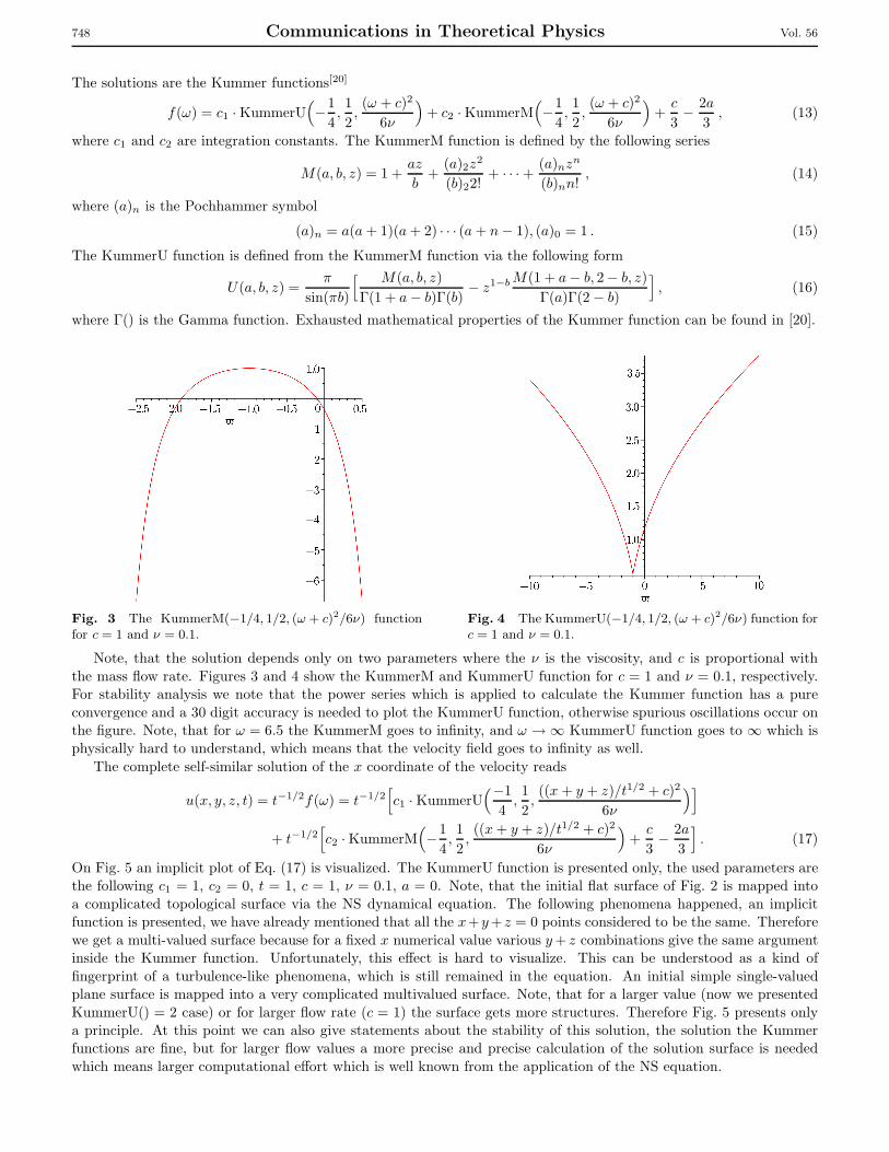
Fig. 3 The KummerM(−1/4, 1/2, (ω + c)2/6ν) functionfor c = 1 and ν = 0.1.

Fig. 4 The KummerU(−1/4, 1/2, (ω + c)2/6ν) function forc = 1 and ν = 0.1.

Note, that the solution depends only on two parameters where the ν is the viscosity, and c is proportional with

the mass flow rate. Figures 3 and 4 show the KummerM and KummerU function for c = 1 and ν = 0.1, respectively.For stability analysis we note that the power series which is applied to calculate the Kummer function has a pure

convergence and a 30 digit accuracy is needed to plot the KummerU function, otherwise spurious oscillations occur onthe figure. Note, that for ω = 6.5 the KummerM goes to infinity, and ω → ∞ KummerU function goes to ∞ which isphysically hard to understand, which means that the velocity field goes to infinity as well.

The complete self-similar solution of the x coordinate of the velocity reads

u(x, y, z, t) = t−1/2f(ω) = t−1/2[

c1 · KummerU(−1

4,1

2,((x + y + z)/t1/2 + c)2

6ν

)]

+ t−1/2[

c2 · KummerM(

−1

4,1

2,((x+ y + z)/t1/2 + c)2

6ν

)

+c

3− 2a

3

]

. (17)

On Fig. 5 an implicit plot of Eq. (17) is visualized. The KummerU function is presented only, the used parameters arethe following c1 = 1, c2 = 0, t = 1, c = 1, ν = 0.1, a = 0. Note, that the initial flat surface of Fig. 2 is mapped into

a complicated topological surface via the NS dynamical equation. The following phenomena happened, an implicitfunction is presented, we have already mentioned that all the x+y+z = 0 points considered to be the same. Therefore

we get a multi-valued surface because for a fixed x numerical value various y+ z combinations give the same argumentinside the Kummer function. Unfortunately, this effect is hard to visualize. This can be understood as a kind of

fingerprint of a turbulence-like phenomena, which is still remained in the equation. An initial simple single-valuedplane surface is mapped into a very complicated multivalued surface. Note, that for a larger value (now we presented

KummerU() = 2 case) or for larger flow rate (c = 1) the surface gets more structures. Therefore Fig. 5 presents onlya principle. At this point we can also give statements about the stability of this solution, the solution the Kummerfunctions are fine, but for larger flow values a more precise and precise calculation of the solution surface is needed

which means larger computational effort which is well known from the application of the NS equation.

No. 4 Communications in Theoretical Physics 749

From the integrated continuity equation (f = c− g− h) we automatically get an implicit formula for the other twovelocity components

v(x, y, z, t) + w(x, y, z, t) = −t−1/2[

c1 · KummerU(−1

4,1

2,((x + y + z)/t1/2 + c)2

6ν

)]

− t−1/2[

c2 · KummerM(

−1

4,1

2,((x+ y + z)/t1/2 + c)2

6ν

)

+c

3− 2a

3

]

+ c . (18)

For explicit formulas of the remaining two velocity components the two ODEs of (11) have to be integrated. Forv(x, y, z, t) = t−1/2g(ω) the ODE is the following

−3νg′′(ω) + g′(ω)(

−ω2

+ c)

− g(ω)

2+ F (f ′′(ω), f ′(ω), f(ω)) = 0 , (19)

where F (f ′′(ω), f ′(ω), f(ω)) contains the combination of the first and second derivatives of the Kummer functions.This is a second order linear ODE and the solution can be obtained with the following general quadrature

g(ω) =[

c2 +

∫

{−c1 +∫

F (f ′′(ω), f ′(ω), f(ω))dω · exp((−ω2/4 + cω)/−3ν)

3ν

}

dω]

exp(−ω2/4 + cω

3ν

)

. (20)

For the sake of simplicity we present the formulas of the first and second derivatives of the KummerU functions only

d

dωKummerU(a, b, ω) =

(ω + a− b)KummerU(a, b, ω) − KummerU(a− 1, b, ω)

ω, (21)

d2

dω2KummerU(a, b, ω) =

1

ω2[a{ωaU(a+ 1, b, ω) − ωU(a+ 1, b, ω)b+ ωU(a+ 1, b, ω)

− aU(1 + a, b, ω)b+ U(a, b, ω)b+ U(a+ 1, b, ω)b2 − U(a+ 1, b, ω)b}] . (22)

Unfortunately, we could not find any closed form for

v(x, y, z, t) and for w(x, y, z, t). Only v the x coordinate

of the velocity v field can be evaluated in a closed form.

Fig. 5 The implicit plot of the self-similar solutionEq. (17). Only the KummerU function is presented fort = 1, c1 = 1, c2 = 0, a = 0, c = 1, and ν = 0.1.

As we mentioned at the beginning there are analytic

solutions available in the literature which are very simi-

lar to our one. Fushchich et al.[3] presented 19 different

solutions for the full three dimensional NS and continuity

equation. (For a better understanding we used the same

notation here as well). For the last (19th) solution they

apply the following Ansatz of

u(z, t) =f(ω)√t, v(y, z) =

g(ω)√t

+y

t,

w(z, t) =h(ω)√t, p(t, z) =

l(ω)√t, (23)

where ω = z/√t is the invariant variable. The obtained

ODE is very similar to ours (9)

h′(ω) + 1 = 0 ,

−1

2(f(ω) + ωf ′(ω)) + h(ω)f ′(ω) = f ′′(ω) ,

1

2(g(ω) + ωg′(ω)) + h(ω)g′(ω) = g′′(ω) ,

−1

2(h(ω) + ωh′(ω)) + h(ω)h′(ω) + l′(ω) = f ′′(ω) . (24)

The solutions are

f(ω) =(3

2ω − c

)

−1/2

exp[

−1

6

(3

2ω − c

)2]

w

×[

− 1

12,1

4,1

3

(3

2ω − c

)2]

,

g(ω) =(3

2ω − c

)

−1/2

exp[

−1

6

(3

2ω − c

)2]

w

×[

− 5

12,1

4,1

3

(3

2ω − c

)2]

,

h(ω) = −ω + c, l(ω) =3

2cω − ω2 + c1 , (25)

where w is the Whitakker function, c and c1 are in-tegration constant. Note that the Whitakker and theKummer functions are strongly related to each other (seeEq. (13.1.32) of Ref. [20]),

w(κ, µ, z) = e−1/2zz1/2+µKummerM

× (1/2 + µ− κ, 1 + 2µ, z) . (26)

More details can be found in the original work.[3]

As a second comparison we show the results of [4].They also have a modified form of (2) which is the follow-

750 Communications in Theoretical Physics Vol. 56

ing

U1t + cU1 + U2U1y + U3U1z − ν(U1yy + U1zz) = 0 ,

U2t + U2U2y + U3U2z + πy − ν(U2yy + U2zz) = 0 ,

U3t + U2U3y + U3U3z + πz − ν(U3yy + U3zz) = 0 ,

U2y + U3z + c = 0 , (27)

where Ui, i = 1 · · · 3 are the velocity components Ui(y, z, t)and π is the pressure, c stands for constants, ν is viscosity,and additional subscripts mean derivations. After sometransformation they get a linear PDA as follows

U1t + k1yU1y + (σ − k1z)U1z − ν(U1yy +U1zz) = 0 , (28)

it is convenient to look the solution in the form of

U1 = Y (y)T (z)Φ(t) . (29)

Note, that they also consider the full 3-dimensional prob-lem, but the velocity field has a restricted two-dimensional(y, z) coordinate dependence. There are additional condi-tions but the general solution can be presented

Φ = c1 exp(c2)t ,

Y = c3M(

−c4,1

2,y2

2ν

)

+ yc5M(1

2− c4,

3

2,y2

2ν

)

,

T ≈M(

c6,1

2,z2

2ν

)

+ zM(1

2− c6,

3

2,z2

2ν

)

, (30)

where M is the KummerM function as presented below.The exact solution in [4] [Eqs. (4.10a)∼(4.10c)] containsmore constants as presented here. It is not our goal to re-produce the full calculation of [4] (which is not our work)we just want to give a guideline to their solution vigor-ously emphasising that our solution is very similar to the

presented one. Note that in both results the arguments of

the KummerM function (13) and (30) are proportional tothe square of the radial component divided by the viscos-ity, additionally one of the parameters is 1/2. As a lastword we just would like to say, (as this example clearlyshows) that the Lie algebra method is not the exhaustive

method to find all the possible solutions of a PDA.

We introduced and gave a geometrical interpretationof a three-dimensional self-similar Ansatz. We applied itto the three-dimensional Navier–Stokes equation in Carte-

sian coordinates. The question of another Ansatze wasmentioned briefly as well. Some part of the results couldbe written as Kummer functions. Unfortunately, someother parts of the results could not be written in closedforms. Further work is in progress, (we still have some

hope) to learn something new from Eq. (19). We com-pared our results with other analytic solutions obtainedfrom various Lie algebra studies. The structure of the re-sult - the implicit coordinate dependence of the Kummer

function - was analyzed as well. We hope that even thismoderate result can give any simulating impetus to theinvestigation of the Navier–Stokes equation. Our solutioncan have some real interest and can be used as a test casefor various numerical methods or commercial computer

packages like Fluent or CFX.

Acknowledgments

The paper is dedicated to my first mathematics teacher“Sanyi Bacsi”.

References

[1] Y. Manwai, J. Math. Phys. 49 (2008) 113102.

[2] V.N. Grebenev, M. Oberlack, and A.N. Grishkov, J. Non-lin. Math. Phys. 15 (2008) 227.

[3] W.I. Fushchich, W.M. Shtelen, and S.L. Slavutsky, J.Phys. A: Math. Gen. 24 (1990) 971.

[4] V. Grassi, R.A. Leo, G. Soliani, and P. Tempesta, Physica286 (2000) 79, ibid, 293 (2000) 421.

[5] X.R. Hu, Z.Z. Dong, F. Huang, et al., Z. NaturforschungA 65 (2010) 504.

[6] S.N. Aristov and A.D. Polyanin, Russ. J. Math. Phys. 17

(2010) 1.

[7] L. Sedov, Similarity and Dimensional Methods in Me-

chanics, CRC Press (1993), see p. 120.

[8] X.Y. Jiao, Commun. Theor. Phys. 52 (2009) 389.

[9] K. Fakhar, T. Hayat, C. Yi, and N. Amin, Commun.Theor. Phys. 53 (2010) 575.

[10] H.Y. Wu, J.X. Fei, and C.L. Zheng, Commun. Theor.Phys. 54 (2010) 55.

[11] C. Dai, Y. Wang, and C. Yan, Optics Communications283 (2010) 1489.

[12] Y. Gao and S.Y. Lou, Commun. Theor. Phys. 52 (2009)1031.

[13] G.I. Baraneblatt, Similarity, Self-Similarity, and Inter-

mediate Asymptotics, Consultants Bureau, New York(1979).

[14] Ya. B. Zel’dovich and Yu. P. Raizer, Physics of Shock

Waves and High Temperature Hydrodynamic Phenomena,Academic Press, New York (1966).

[15] J. Leray, Acta Math. 63 (1934) 193.

[16] J.R. Miller, M. O’Leray, and M. Schonbeck, Math. Ann.319 (2001) 809.

[17] B.H. Gilding and R. Kersner, Travelling Waves in Non-

linear Diffusion-Convection Reactions, in Progress in

Nonlinear Differential Equations and Their Applications,Birkhauser Verlag, Basel-Boston-Berlin (2004).

[18] I.F. Barna and R. Kersner, J. Phys. A: Math. Theor. 43

(2010) 375210.

[19] I.F. Barna and R. Kersner, Adv. Studies Theor. Phys. 5

(2011) 193.

[20] M. Abramowitz and I. Stegun, Handbook of Mathematical

Functions, Dover Publication Inc., New York (1968).