Self-sorting, incentive compensation and human-capital · PDF fileSelf-sorting, incentive compensation and ... Not estimating a value for human capital and not recognizing it ... incentive

European Accounting Review 2003, 12:4, 661–697

Self-sorting, incentive compensation andhuman-capital assets

A. Rashad Abdel-khalik

University of Illinois at Urbana-Champaign

ABSTRACT

Skilled labour has gained significance as a production factor in the age of informationtechnology, but accounting does not recognize human capital as an asset thatcontributes to the firm’s earning power. This paper suggests a method to develop alatent index to proxy the managerial-skill component of human capital. The proposedindex depends on the empirical validity of self-sorting theories for managerial tasks andthe choice of the type of at-risk (i.e. outcome-contingent) compensation contract. Theempirical analysis uses data on compensation of executive members of the board ofdirectors, their personal attributes (experience, risk aversion and wealth), firm-specificvariables ( profitability growth rates, organizational complexity and operating risk), andtype of industry. The extent to which equity markets value the predicted labour skillsshows that investors in the marketplace recognize human capital even thoughaccounting does not. The valuation coefficient on the variable imputed for humancapital is significant for all years examined. This study contributes to the literature byshowing that relative incentive compensation (incentive pay per dollar of fixed salary) isa viable surrogate for human capital defined as the skills embodied in people.

1. INTRODUCTION

Consistent with the literature in economics, Topel (2000) defines human capital

as ‘the intangible stock of skills that are embodied in people’. Using this

definition, this study examines human capital from the employers’ point of

view and provides a method that uses incentive compensation to develop a

relative index for managerial skills. The proposed index derives from super-

imposing an incentive–compensation structure on a Cobb–Douglas production

function and is estimated using variables for the individual manager (experience,

risk preference, value of owned shares as proxy for personal wealth) and firm-

specific variables that reflect managerial performance ( past performance on profit

and growth, organizational complexity and operating risk). Once the index is

Address for correspondence

A. Rashad Abdel-khalik, V. K. Zimmerman Center for International Education and

Research in Accounting, 320 Wohlers Hall, 1206 South Sixth Street, Champaign, IL61820, USA. E-mail: [email protected]

Copyright # 2003 European Accounting Association

ISSN 0963-8180 print=1468-4497 online DOI: 10.1080=09638180310001628428

Published by Routledge Journals, Taylor & Francis Ltd on behalf of the EAA

estimated, the question of valuation arises. While economists view human capital

as the skill that can be estimated by the life cycle earning capacity of the

individual, accountants are more interested in measuring human capital as a

resource to the employer. In neither case, however, is the methodology for placing

dollar values on human capital well developed because the skills embodied in

humans are inherently difficult to measure. In this study I address the accounting

valuation problem only to explain the extent to which capital markets implicitly

recognize labour skills when pricing a firm’s equity.

In the empirical analysis I estimate the index of labour skills for executive

members of the board of directors who are employees of the firm. The data were

obtained from ExecuComp, Compustat and CRSP databases for the period 1996–

2000. The number of firms included in the sample varied by year due to the

availability of data and to the selection criterion that required some stability of

management regimes. Data requirements were satisfied for 617 firms for the years

1996 to 1998, and for 520 firms for the years 1998 to 2000. Because of the

inherent serial dependency of the data, the analysis is carried out for different sub-

samples. I first estimate the models and perform predictions and valuation

separately for each year at three different levels: (1) for the CEO’s position,

(2) for other executives (firm employees) who are members of the board of

directors (Oexecs), and (3) for the pooled data set. I then repeat this analysis to

check for robustness: (1) using three randomly selected portfolios (of 15%, 20%

and 30% of the pooled time-series=cross-section data panel); (2) using proxy for

labour skills as a binary, indicator variable; and (3) using a different valuation

model.

The results are consistent with the predictions of the model in that (1) the

variables of risk preference, value of owned shares, organizational complexity,

profitability, growth rates and firm operating risk are significantly related to the

proposed latent index of human-capital; and (2) the forward predictions of that

index are significantly associated with the market’s valuation of common equity.

These findings are reproduced even after transforming the estimated human

capital variable from ratio-scale data into a binary indicator variable.

2. THE RESEARCH DESIGN

The research problem of interest relates to two research questions: (1) How could

this intangible human-capital resource be estimated as an asset? (2) Do capital

markets impute a value to that asset? The relevance of these research questions

arises from the dramatic effects of information technology on the mix of

production factors in developed economies during the last quarter of the twentieth

century. It appears that wealth creation is driven more by human innovations, new

product inventions and fast communication than by tangible assets. The unpre-

cedented advances in microchip technology and programming skills have

significantly impacted every aspect of society, contributed to lowering transaction

662 European Accounting Review

costs, and allowed enterprises to locate their activities in regions with lower

operating costs.

Empirical evidence shows that

[T]he shift toward more skilled workers appears to have accelerated in the last 25 yearsrelative to 1940–1973, especially over the period from 1980 until the mid-1990s. Overthis period, demand has strongly shifted from low-and-middle-wage occupations andskills toward highly rewarded jobs and tasks, those requiring exceptional talent, training,autonomy, or management ability.

(Bresnahan et al., 2002: 339)

Similar findings are noted in numerous other studies. For example, in a cross-

sectional analysis, Doms et al. (1997) find that ‘plants that use a large number of

new technologies employ more educated workers, employ relatively more

managers, professionals and precision-craft workers, and pay higher wages’

(1997: 255). Evidently, these developments are related to the talents of the

labour force. Indeed, successful firms manage their business based on the

knowledge that human skills are the resources that power the enterprise’s earnings

capacity.

While human resources management has progressed in recent years to adapt to

these changes in the business environment, accounting systems have not.

Consequently, economic resources such as software programming skills at

Microsoft or the expertise in microchip technology at Intel are omitted from

the set of recognized assets. For these types of firms, human capital is their most

important asset. Not estimating a value for human capital and not recognizing it

as an economic resource distort both amounts and relationships among the

elements of financial statements. This brings us to the second research question.

Notwithstanding accounting shortcomings, do capital markets value the quality of

the labour force? If markets do value the firm’s labour skills, it would be

tantamount to market recognition of human capital even though accountants do

not recognize it on the balance sheet.

To motivate the research questions, self-sorting theory in labour markets

provides a framework to show that employees reveal their skills by their choice

of compensation contracts. The more skilled employees select contracts with a

higher proportion of performance-based (i.e. at-risk) compensation and earn, on

average, higher compensation than others. Consistent with self-sorting, an index

for relative incentive compensation is shown to be a function of operating

(tangible) capital and labour skills. The index is obtained by relating the structure

of compensation contracts to performance, with performance being measured

as the output represented by a Cobb–Douglas production function. In this

formulation, labour skills are substituted for the labour factor and are proxied

by variables that contribute to the individual’s capacity to perform and earn

income. These proxy variables are of two types: individual-related (experience,

risk preference and wealth surrogate) and firm-specific (history of profitability,

growth and the operating risk of the enterprise).

Self-sorting, incentive compensation and human-capital assets 663

To obtain a single proxy for labour skills, and test the identification hypothesis,

I introduce the proposed Cobb–Douglas production function into a compensation

contract so that relative incentive pay (RIC) could be expressed in terms of both

tangible assets and the proxy for labour skills. RIC is defined as the ratio of

performance-based compensation to base salary. However, we know that the

incentive component of the exercised options is related to contemporaneous

market prices of equity. The endogeneity of RIC with firm performance led to

separation between estimation and valuation periods; labour skills index is

estimated in one period and is predicted for another period, with the predicted

index being used for testing the valuation hypothesis in the latter period. The

predicted index is based on factors other than market prices. Furthermore, the

predicted index is not derived directly from the RIC measures generated during

the periods in which market prices are used for testing hypotheses. With reducing

the threat of obtaining spurious relationships by the methods described above, the

predicted proxy for labour skills is then used to test the following two hypotheses:

H1: Identification: Human capital factors (experience, risk aversion

and value of owned shares (surrogate for wealth)) are significant

determinants of relative incentive compensation:H2: Valuation: Equity markets recognize and value the latent index of

managerial (or labour) skills imputed from information on human

capital factors and relative incentive compensation:

3. OVERVIEW OF THE LITERATURE

The recent interest in studying human capital evolved from the broader concept of

intellectual capital. As noted from the concept’s inception in Europe (Edvinsson

and Malone, 1997), intellectual capital is assumed to encompass human capital,

organizational capital and customer capital (see also Petty and Guthrie, 2000;

Lev, 2001). This interest appears to be motivated, in part, by the need to explain

the apparent large growth of unrecognized intangible assets. Large increases in

market-to-book ratios in the past three decades provide evidence of this growth.

Mouritsen et al. (2001) emphasize the role of increasing market-to-book ratio in

reflecting omitted intangibles. They show how seventeen Danish companies

report intellectual-capital statements in an effort to collaborate with the Danish

Agency for Development of Trade and Industry in developing guidance for this

type of reporting (Mouritsen et al., 2001: 741–2). These projects are components

of the MERITUM co-operative program involving the efforts of researchers in

different EU countries to study intangibles. The governments of several European

nations (e.g. Spain and the Scandinavian countries) are actively involved in this

development.

The setting in North America is different. The debate on the recognition of

human capital as an asset on the firm’s balance sheet dates back to the 1960s and

1970s, but since that time there has been only a modest revival of interest in the


problem. Until the mid-1970s, authors (e.g. Brummet et al., 1968; Flamholtz,

1969, 1971, 1999; Lev and Schwartz, 1971; Likert and Pyle, 1971; Elias, 1972;

Likert and Bowers, 1973; Morse, 1973; Friedman and Lev, 1974; Sackman et al.,

1985) proposed various methods for estimating and reporting human capital on

the employer’s balance sheet. Invariably, these methods consist of capitalizing

some expected flow: lifetime income, the firm’s abnormal earnings or the cost of

recruiting and training personnel. However, dissenters like Dittman et al. do not

share that view. They write: ‘we are personally not convinced of the importance

of human-asset accounting in external reports and the propriety of ‘‘putting

people on your balance sheet’’’ (1976: 62). Dittman et al. argue that different

functions require different measures of human resources and that the arguments

underlying reporting human capital hinge on simplistic assumptions. Never-

theless, the enthusiasm about human resources during the early 1970s led R. G.

Barry, Inc., a then US publicly-traded firm, to experiment with reporting an asset

value for human capital on its balance sheet (Caplan and Landekich, 1973;

Flamholtz, 1999). But, in the US environment, there is no current or extensive

experimentation of the type undertaken in Denmark as discussed in Mouritsen

et al. (2001).

Although most researchers agree that human capital is the stock of labour skills

embodied in people, authors use the term ‘human capital’ in different contexts to

connote different concepts. In particular, there is difference between (1) the rights

a person has to her or his own earnings (the life cycle theory), and (2) the rights

of the employer to excess profits generated by investing in human resources.

The former uniquely belongs to the individual, while the latter is a property of

the firm.

The accounting approaches of the 1960s and 1970s are generally consistent

with the view that the employer firm could only claim the benefits that accrue to

it from developing and investing in human resources. Additionally, in this

context, the fair value of the firm’s claim to human-capital assets would be

estimated like any other asset by the present value of its expected contribution to

the firm’s future earnings. This value would be estimated based on cash flows to

be earned by the firm, not the individual. Thus, economists and accountants study

human capital in different contexts and for different objectives.

The early debate on the accounting recognition of human capital ended without

closure not because of confusion about who owns what aspect of human capital,

but more likely because ‘people and [information] technology were significantly

less important to wealth creation in 1960s and 1970s’ (Albert and Bradley, 1997:

68). As these issues have grown in importance, researchers have returned to

studying the problem.

Currently, researchers highlight the value relevance of intangibles by examin-

ing the association between some surrogates for omitted assets and equity market.

Some of these unrecognized assets contribute to creating human capital. For

example, Sougiannis (1994) considers the omitted asset of R&D, and Aboody

and Lev (1998) examine the value relevance of the omitted asset of software


developments. Few studies, however, have examined the value relevance of human

capital, mostly because of the complexity of identification and measurement

problems. Jagannathan et al. (1998) and Rosett (2001) examine the association

between labour cost and equity risk, whereas Hansson (2001) uses data from the

Swedish Stock Exchange to examine the different effects of growth in wages on

equity returns for two types of firms categorized by book-to-market ratios: value-

stock firms and growth-stock firms. In a different context, Amir and Livne (2002)

examine data from football clubs to evaluate the returns to investing in human

capital. They conclude, ‘information about investment in human capital may be

useful to investors and potentially capable of being accounted for as an asset’

(2002: 2). The uniqueness of the Amir–Livne application lies in using actual

prices paid to athletes, although no valuation is generated for the skills developed

internally. Furthermore, paying high prices for football players limits their

freedom to self-sort because these contracts do not allow players to re-enter the

marketplace and, as a result, could contract only once.

4. LABOUR SKILL LEVELS AS A LATENT VARIABLE

Self-sorting

In reality, neither the talent (a credence good) nor the skill (credence and

experience good) of an individual is observable. For this reason, the ability of

a manager to lead, produce and affect change can be described in two ways: (1) ex

ante in terms of job duties and specifications, and (2) ex post in relationship to the

employers’ performance as measured against known expectations. The informa-

tion asymmetry between the employer and prospective employees gives rise to a

problem of adverse selection: the employer has incomplete information about the

skill level of any employee who is not yet hired. Therefore, ‘absent any policy of

mitigating this problem, the wrong kind of workers could be attracted to the firm’

(Lazear, 1998: 47).

In practice, business firms use different methods to mitigate the problem of

adverse selection before hiring. They seek resumes and letters of reference, and

conduct interviews with candidates, but labour market studies suggest, ‘one of the

most effective ways to induce the appropriate people to apply for a job is to

structure compensation in a way that is attractive to highly-skilled workers, but

less attractive to unskilled workers’ (Lazear, 1998: 49). That is, firms could design

compensation policies that induce prospective managers to indirectly reveal their

skill levels by their contract choice. Upon learning of the compensation structure

of different firms, those jobseekers who have expertise in specific tasks will

search for employment contracts that would reward their achievements in

performing those tasks well. For example, individuals who have the ability to

devise strategies for increasing market shares will be attracted to work for those

firms that offer contracts to reward them on that basis. Similarly, managers who

have the expertise to increase profitability by cutting costs and undertaking


innovation will seek employment with firms that contract to compensate them for

performance in these areas. In general, one outcome of self-sorting is that

employees are differentially compensated on the basis of their relative abilities.

For example, Lazear concludes that firms that pay piece rate (output-contingent

pay) generally attract higher quality workers and report greater productivity than

those that pay straight salaries (1986, 2000). This process of self-sorting will

continue after employment; the less able workers and those who are not

compensated according to their skills will eventually change employers

(Jovanovic, 1979; Lazear, 1998). In addition, sorting within the organization

might take a different form because of the diminishing problem of adverse

selection. For example, Hvide and Kaplan (2003) develop a model in which

delegation of job design within the firm allows high-ability workers to signal their

ability by choosing different tasks.

Sorting theories have been used to analyse differential wages for different

groups (e.g. male=female: Groshen, 1991) or different skills. But in the account-

ing literature only Raviv (1985) has raised this concept in his discussion of the

association between incentive-plan adoptions for executives and shareholders’

wealth. He made two pertinent points concerning the need to address the

consequences of self-sorting, and the difficulty of disentangling the effect of

self-sorting from the incentive to reduce agency cost. Self-sorting in labour

markets, however, is a pre-contracting process whose post-contracting effect

would be to align the interests of both stockholders and owners in two ways:

(1) improving productivity by matching job requirements and hired skills, and

(2) compensating managers based on their relative performance.

Two conditions are necessary for the labour market to effectively match the

interests of employees and employers: (1) employers need to disclose their

compensation policies, and (2) prospective employees must be able to estimate

their expected compensation under alternative schemes. Employers and prospec-

tive employees, therefore, have the incentive to produce and search for informa-

tion that would enhance sorting and job matching (MacDonald, 1980). In this

respect, one could argue that enhancing the pool of information available to the

public about the structure of executive compensation policies is a beneficial

externality of some recent accounting regulations (e.g. the Financial Accounting

Standards Board; FAS 123, 1995). This particular data source is of value in the

research design discussed next.

Performance-based compensation and labour skills

I benefited in this study by the research and empirical evidence on job selection

and incentives for employees who perform tasks that are less complex than the

tasks of top management. I assume in this study that the concepts found to hold in

the labour market for other skills will also apply in the managerial markets, and

further assume that, on average, managerial skills map onto relative compensation.

It follows then that the information on incentive compensation could be used to


infer the corresponding unobservable intangible. To show how this inference

might be drawn, assume a simple Cobb–Douglas production function of the form

y ¼ BKaL1�aeey (1)

where y is output, B is a constant, K is tangible capital (productive assets other

than labour), L is labour, a is the elasticity (marginal productivity) of capital, and

(17 a) is the elasticity (marginal productivity) of labour, with 0< a< 1, and ey is

a random error term with an assumed standard normal distributional property

N(0, sy). The usual assumption is that the firm’s goal is to maximize profits and is

therefore operating in the region of decreasing returns to scale.1

Labour as a factor of production has two components: quantity (i.e. number

of input hours) and quality (i.e. skill). Since labour hours are not homogeneous

in skills, it would be more descriptive to substitute a skill-weighted variable, LS,

for L. Making this substitution in (2) and taking the log of both sides, we have

the linear function

ln y ¼ lnBþ a lnK þ (1 � a) ln LS þ ey (2)

Of the two production factors, only capital, lnK (e.g. tangible assets), is empi-

rically available while ln LS has to be estimated or imputed. In this study, log total

assets are used for ln K.

In general, any compensation policy in an agency is reducible to two primary

components: (1) a fixed salary, and (2) at-risk compensation contingent on

performance. If ‘performance’ in this contractual arrangement is related to

expected output y, the basic compensation structure could be described by

C ¼ w0 þ y ln yþ ec (3)

where C is compensation, w0 is base salary (which is endogenous because it is not

independent of the portfolio mix of fixed and contingent pay, but I will assume

that w0 is exogenous for the purpose of developing the model), y is output as

specified in the compensation contract, y is a parameter translating output into

incentive compensation, and ec is a random error term that is N(0, sc). By

substituting (2) into (3), we obtain

C ¼ w0 þ y( lnBþ a lnK þ (1 � a) ln LS þ ey) þ ec (4)

By dividing both sides by w0, we obtain

RIC ¼ 1 þ1

w0

� �y( lnBþ a lnK þ (1 � a) ln LS þ eyÞ þ ec

� �¼ 1 þ m0 lnBþ m1 lnK þ m2 ln LS þ ecy (5a)


where RIC¼C=w0 and is the incentive pay per one dollar of salary,2 an index

of relative incentive compensation; m0¼ y=w0; m1¼ (ya=w0); m2¼ (y(17 a)=w0);

ln K reflect tangible operating capital (i.e. log total assets); ln LS reflect labour

skills; and the error term ecy¼ (yey þ ec)=w0.

It is useful to state one more definition at this point. Because predicted RIC,

which is a ratio, is used to impute a proxy for human capital, the imputed labour-

skills index will also be denominated in a non-monetary scale. Therefore,

assuming ln Lsi is a labour-skills index denominated in non-monetary units, q

is the scalar of converting ln Lsi into dollar amounts, then ln Lsi is a

transformation of ln LS by the scalar q in the form

ln LS ¼ q ln Lsi

and equation (5a) becomes

RIC ¼ 1 þ m0 lnBþ m1 lnK þ m2q ln Lsiþ ecy (5b)

ln Lsi is not available in an archival sense and will be surrogated by proxy

variables. Let these proxy variables be the elements of the set H, and h0 is a row

vector of coefficients on H, then substituting h0(H) for ln Lsi results in

RIC ¼ 1 þ m0 lnBþ m1 lnK þ m2q[h0(H) þ uH ] þ ecy (5c)

where m2q¼ qm2, h0(H )¼E(ln Lsi), uH is the related error resulting from using

the proxy h0(H) for estimation, and other terms are as defined before. The

random-error term uH has N(0, sH) and is uncorrelated with any element in H.

The proxy variables in H are discussed later in this study.

Rearranging (5c) to enable inferring ln Lsi, the human capital component

would be expressed as

h0(H) ¼ E( ln Lsi) ¼1

m2q

![RIC � m0 lnB� m1 lnK � 1 � ecy þ uH ] (6a)

Or, simplifying,

ln Lsi ¼ g1(RIC � 1) � g0 lnB� g2 lnK þ ecyh (6b)

where g0¼ (m0=m2q); g1¼ (1=m2q); g2¼ (m1=m2q); and ecyh is the sum of the two

random terms and is assumed N(0, s(ecyh)).As indicated earlier, RIC is a relative incentive pay index and ln K is log total

assets, both of which could be obtained from empirically available data.3 If values

of ln Lsi were available, empirical assessment of the relationship in (6) would be

equivalent to estimating reverse regressions (Maddala, 1988). Estimating ln Lsi


will require estimating (6b) using proxies for human capital as is discussed below.

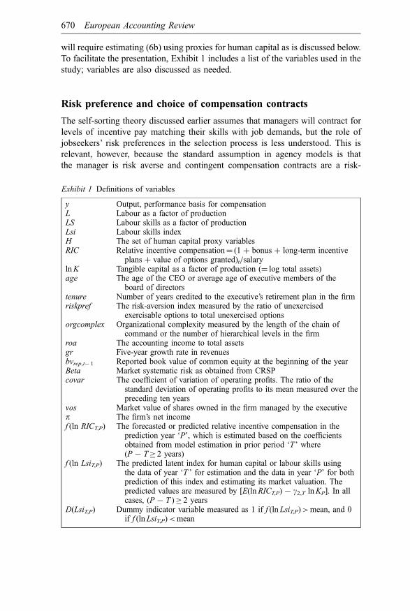
To facilitate the presentation, Exhibit 1 includes a list of the variables used in the

study; variables are also discussed as needed.

Risk preference and choice of compensation contracts

The self-sorting theory discussed earlier assumes that managers will contract for

levels of incentive pay matching their skills with job demands, but the role of

jobseekers’ risk preferences in the selection process is less understood. This is

relevant, however, because the standard assumption in agency models is that

the manager is risk averse and contingent compensation contracts are a risk-

Exhibit 1 Definitions of variables

y Output, performance basis for compensationL Labour as a factor of productionLS Labour skills as a factor of productionLsi Labour skills indexH The set of human capital proxy variablesRIC Relative incentive compensation¼ (1 þ bonus þ long-term incentive

plans þ value of options granted)t=salarylnK Tangible capital as a factor of production (¼ log total assets)age The age of the CEO or average age of executive members of the

board of directorstenure Number of years credited to the executive’s retirement plan in the firmriskpref The risk-aversion index measured by the ratio of unexercised

exercisable options to total unexercised optionsorgcomplex Organizational complexity measured by the length of the chain of

command or the number of hierarchical levels in the firmroa The accounting income to total assetsgr Five-year growth rate in revenuesbvrep,t�1 Reported book value of common equity at the beginning of the yearBeta Market systematic risk as obtained from CRSPcovar The coefficient of variation of operating profits. The ratio of the

standard deviation of operating profits to its mean measured over thepreceding ten years

vos Market value of shares owned in the firm managed by the executivep The firm’s net incomef (ln RICT,P) The forecasted or predicted relative incentive compensation in the

prediction year ‘P’, which is estimated based on the coefficientsobtained from model estimation in prior period ‘T’ where(P7 T� 2 years)

f (ln LsiT,P) The predicted latent index for human capital or labour skills usingthe data of year ‘T ’ for estimation and the data in year ‘P’ for bothprediction of this index and estimating its market valuation. Thepredicted values are measured by [E(lnRICT,P)7 g2,T lnKP]. In allcases, (P7T )� 2 years

D(LsiT,P) Dummy indicator variable measured as 1 if f (ln LsiT,P)>mean, and 0if f (ln LsiT,P)<mean


sharing mechanism. The executive, however, does not have full control over

the realization of the outcome basis of the compensation contingency (i.e.

output or performance). In general, rational individuals (who are risk averse)

would bear risk if paid an appropriate risk premium. The choice of form and

extent of at-risk compensation will depend on the manager’s risk-bearing

propensity.

It is, however, very difficult to empirically estimate risk preferences of

individuals, especially those who are members of boards of directors. The

existing empirical measures on estimating risk aversion have been generated

experimentally by evaluating the investment and consumption habits of indivi-

duals. The instrument of a typical survey or experiment requests that subjects

price a gamble or a pair of gambles. Hartog et al. (2000) use data from three

surveys of pricing hypothetical lotteries completed by over 23,000 individuals

(including 1,599 chartered accountants) to test the respondents’ risk aversion.

They find that, for all participants including the accountants, risk aversion

declines with income and wealth. Similarly, Donkers et al. (2001) estimate risk

aversion from the responses to hypothetical questions about lotteries contained in

survey data about the saving habits of 2,780 Dutch households. Loehman (1998)

elicited the pricing of a gamble of paired lotteries, while Schooley and Worden

(1996) used the ratio of risky assets to wealth based on survey results of 3,143

households.

In non-experimental articles, Guay (1999) and Rogers (2002) use the ratio of

options’ vega to delta as a determinant of managing risk. Vega is the ratio of the

change in the value of options to the change in volatility, and delta is the change

in the value of options to the change in the value of the underlying asset or

parameter (i.e. interest rate). Thus, the ratio of vega to delta is the average change

in volatility to average change in the underlying asset or parameter. It is noted that

neither one of these two factors is a personal choice of the executive, especially

since executive stock options have no market. A different method of estimating

risk preference is used in this study.

The measure of risk preference used in this study relies on individual choices

of income and wealth made by executives. At any time stock options held by

executives are either exercisable (vested) and in the money, or unvested and not

exercisable. To exercise or defer exercising in-the-money vested options is largely

an individual choice. If deferral is assumed to take place only in anticipation of

higher stock prices and higher future compensation,4 the magnitude of deferred

vested (in-the-money) options would be an indicator of the manager’s willingness

to bear risk; deferral entails sacrificing a sure current gain for the prospect of

expected higher gains at a future date. In this sense, deferring exercising in-the-

money vested options is equivalent to purchasing a lottery ticket; its price is the

compensation that could be earned if the options were exercised (i.e. current

sacrifice) and the prize is the expected gain in the future. Holding a larger

proportion of vested options implies a relatively greater inclination toward risk

bearing, and vice versa. The executive’s risk preference (riskpref ) is therefore


measured in this study by the proportion of (unexercised) vested and exercisable

(in-the-money) options to total (in-the-money) options held. A relatively high

riskpref score reveals an executive with a relatively low risk aversion who would

also accept greater risk sharing; i.e. relatively more at-risk pay. In contrast, a low

riskpref score points to an executive with a relatively high risk aversion who

prefers less risk sharing; i.e. would demand relatively higher salary and low at-

risk pay. Given this definition, one would expect a positive association between

risk-preference scores and RIC (relative incentive pay index).

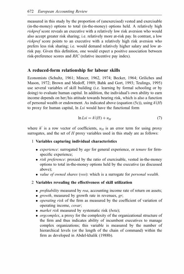
A reduced-form relationship for labour skills

Economists (Schultz, 1961; Mincer, 1962, 1974; Becker, 1964; Griliches and

Mason, 1972; Brown and Medoff, 1989; Bahk and Gort, 1993; Teulings, 1995)

use several variables of skill building (i.e. learning by formal schooling or by

doing) to evaluate human capital. In addition, the individual’s own ability to earn

income depends on her=his attitude towards bearing risk, which is also a function

of personal wealth or endowment. As indicated above (equation (5c)), using h0(H)

to proxy for human capital, ln Lsi would have the functional form

ln Lsi ¼ h0(H) þ uH (7)

where h0 is a row vector of coefficients, uH is an error term for using proxy

surrogates, and the set of H proxy variables used in this study are as follows:

1 Variables capturing individual characteristics

� experience: surrogated by age for general experience, or tenure for firm-

specific experience;

� risk preference: proxied by the ratio of exercisable, vested in-the-money

options to total in-the-money options held by the executive (as discussed

above);

� value of owned shares (vos): which is a surrogate for personal wealth.

2 Variables revealing the effectiveness of skill utilization

� profitability measured by roa, accounting income rate of return on assets;

� growth, measured by growth rate in revenues, gr;

� operating risk of the firm as measured by the coefficient of variation of

operating income, covar;

� market risk measured by systematic risk (beta);

� orgcomplex, a proxy for the complexity of the organizational structure of

the firm and thus indicates ability of incumbent executives to manage

complex organizations; this variable is measured by the number of

hierarchical levels (or the length of the chain of command) within the

firm as developed in Abdel-khalik (1988b).


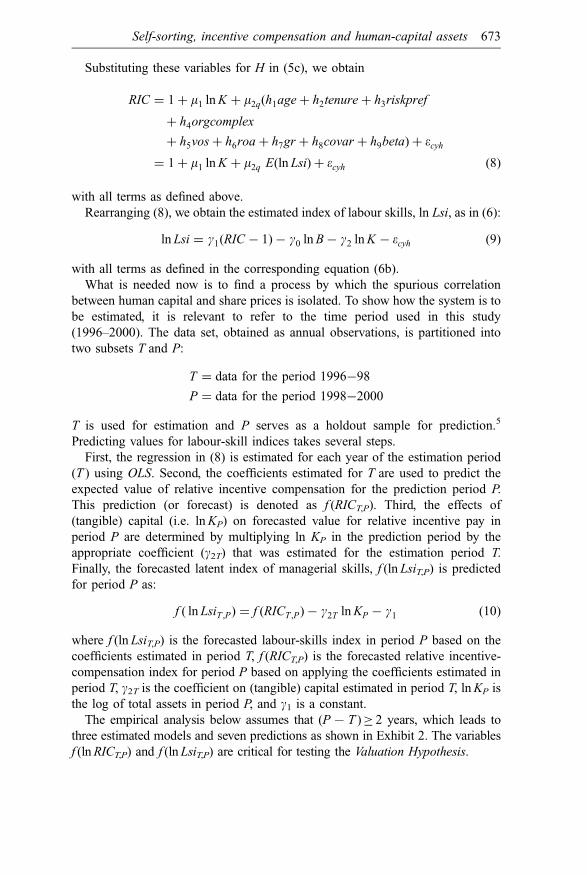
Substituting these variables for H in (5c), we obtain

RIC ¼ 1 þ m1 lnK þ m2q(h1ageþ h2tenureþ h3riskpref

þ h4orgcomplex

þ h5vosþ h6roaþ h7gr þ h8covar þ h9beta) þ ecyh¼ 1 þ m1 lnK þ m2q E(ln Lsi) þ ecyh (8)

with all terms as defined above.

Rearranging (8), we obtain the estimated index of labour skills, ln Lsi, as in (6):

ln Lsi ¼ g1(RIC � 1) � g0 lnB� g2 lnK � ecyh (9)

with all terms as defined in the corresponding equation (6b).

What is needed now is to find a process by which the spurious correlation

between human capital and share prices is isolated. To show how the system is to

be estimated, it is relevant to refer to the time period used in this study

(1996–2000). The data set, obtained as annual observations, is partitioned into

two subsets T and P:

T ¼ data for the period 1996�98

P ¼ data for the period 1998�2000

T is used for estimation and P serves as a holdout sample for prediction.5

Predicting values for labour-skill indices takes several steps.

First, the regression in (8) is estimated for each year of the estimation period

(T ) using OLS. Second, the coefficients estimated for T are used to predict the

expected value of relative incentive compensation for the prediction period P.

This prediction (or forecast) is denoted as f (RICT,P). Third, the effects of

(tangible) capital (i.e. lnKP) on forecasted value for relative incentive pay in

period P are determined by multiplying ln KP in the prediction period by the

appropriate coefficient (g2T) that was estimated for the estimation period T.

Finally, the forecasted latent index of managerial skills, f (ln LsiT,P) is predicted

for period P as:

f ( ln LsiT ,P) ¼ f (RICT ,P) � g2T lnKP � g1 (10)

where f (ln LsiT,P) is the forecasted labour-skills index in period P based on the

coefficients estimated in period T, f (RICT,P) is the forecasted relative incentive-

compensation index for period P based on applying the coefficients estimated in

period T, g2T is the coefficient on (tangible) capital estimated in period T, lnKP is

the log of total assets in period P, and g1 is a constant.

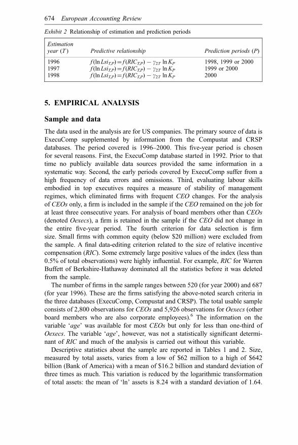
The empirical analysis below assumes that (P7T )� 2 years, which leads to

three estimated models and seven predictions as shown in Exhibit 2. The variables

f (lnRICT,P) and f (lnLsiT,P) are critical for testing the Valuation Hypothesis.


5. EMPIRICAL ANALYSIS

Sample and data

The data used in the analysis are for US companies. The primary source of data is

ExecuComp supplemented by information from the Compustat and CRSP

databases. The period covered is 1996–2000. This five-year period is chosen

for several reasons. First, the ExecuComp database started in 1992. Prior to that

time no publicly available data sources provided the same information in a

systematic way. Second, the early periods covered by ExecuComp suffer from a

high frequency of data errors and omissions. Third, evaluating labour skills

embodied in top executives requires a measure of stability of management

regimes, which eliminated firms with frequent CEO changes. For the analysis

of CEOs only, a firm is included in the sample if the CEO remained on the job for

at least three consecutive years. For analysis of board members other than CEOs

(denoted Oexecs), a firm is retained in the sample if the CEO did not change in

the entire five-year period. The fourth criterion for data selection is firm

size. Small firms with common equity (below $20 million) were excluded from

the sample. A final data-editing criterion related to the size of relative incentive

compensation (RIC). Some extremely large positive values of the index (less than

0.5% of total observations) were highly influential. For example, RIC for Warren

Buffett of Berkshire-Hathaway dominated all the statistics before it was deleted

from the sample.

The number of firms in the sample ranges between 520 (for year 2000) and 687

(for year 1996). These are the firms satisfying the above-noted search criteria in

the three databases (ExecuComp, Compustat and CRSP). The total usable sample

consists of 2,800 observations for CEOs and 5,926 observations for Oexecs (other

board members who are also corporate employees).6 The information on the

variable ‘age’ was available for most CEOs but only for less than one-third of

Oexecs. The variable ‘age’, however, was not a statistically significant determi-

nant of RIC and much of the analysis is carried out without this variable.

Descriptive statistics about the sample are reported in Tables 1 and 2. Size,

measured by total assets, varies from a low of $62 million to a high of $642

billion (Bank of America) with a mean of $16.2 billion and standard deviation of

three times as much. This variation is reduced by the logarithmic transformation

of total assets: the mean of ‘ln’ assets is 8.24 with a standard deviation of 1.64.

Exhibit 2 Relationship of estimation and prediction periods

Estimationyear (T ) Predictive relationship Prediction periods (P)

1996 f (ln LsiT,P)¼ f (RICT,P)7 g2T lnKP 1998, 1999 or 20001997 f (ln LsiT,P)¼ f (RICT,P)7 g2T lnKP 1999 or 20001998 f (ln LsiT,P)¼ f (RICT,P)7 g2T lnKP 2000


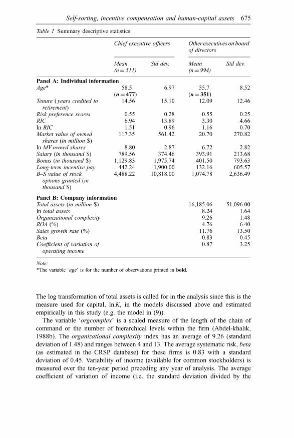
The log transformation of total assets is called for in the analysis since this is the

measure used for capital, lnK, in the models discussed above and estimated

empirically in this study (e.g. the model in (9)).

The variable ‘orgcomplex’ is a scaled measure of the length of the chain of

command or the number of hierarchical levels within the firm (Abdel-khalik,

1988b). The organizational complexity index has an average of 9.26 (standard

deviation of 1.48) and ranges between 4 and 13. The average systematic risk, beta

(as estimated in the CRSP database) for these firms is 0.83 with a standard

deviation of 0.45. Variability of income (available for common stockholders) is

measured over the ten-year period preceding any year of analysis. The average

coefficient of variation of income (i.e. the standard deviation divided by the

Table 1 Summary descriptive statistics

Chief executive officers Other executives on boardof directors

Mean(n¼ 511)

Std dev. Mean(n¼ 994)

Std dev.

Panel A: Individual informationAge* 58.5

(n¼ 477)6.97 55.7

(n¼ 351)8.52

Tenure ( years credited toretirement)

14.56 15.10 12.09 12.46

Risk preference scores 0.55 0.28 0.55 0.25RIC 6.94 13.89 3.30 4.66ln RIC 1.51 0.96 1.16 0.70Market value of ownedshares (in million $)

117.35 561.42 20.70 270.82

ln MV owned shares 8.80 2.87 6.72 2.82Salary (in thousand $) 789.56 374.46 393.91 213.68Bonus (in thousand $) 1,129.83 1,975.74 401.50 793.63Long-term incentive pay 442.24 1,900.00 132.16 605.57B–S value of stockoptions granted (inthousand $)

4,488.22 10,818.00 1,074.78 2,636.49

Panel B: Company informationTotal assets (in million $) 16,185.06 51,096.00ln total assets 8.24 1.64Organizational complexity 9.26 1.48ROA (%) 4.76 6.40Sales growth rate (%) 11.76 13.50Beta 0.83 0.45Coefficient of variation ofoperating income

0.87 3.25

Note:

*The variable ‘age’ is for the number of observations printed in bold.


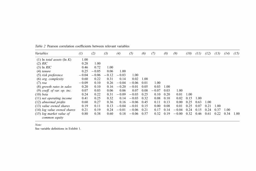
Table 2 Pearson correlation coefficients between relevant variables

Variables (1) (2) (3) (4) (5) (6) (7) (8) (9) (10) (11) (12) (13) (14) (15)

(1) ln total assets (ln K) 1.00(2) RIC 0.28 1.00(3) ln RIC 0.46 0.72 1.00(4) tenure 0.25 �0.05 0.06 1.00(5) risk preference �0.04 �0.06 �0.12 �0.03 1.00(6) org. complexity 0.60 0.22 0.31 0.14 0.02 1.00(7) roa �0.09 0.10 0.26 �0.04 �0.06 0.01 1.00(8) growth rates in sales 0.20 0.10 0.16 �0.20 �0.01 0.05 0.03 1.00(9) coeff. of var. op. inc. 0.07 0.03 0.06 0.06 0.07 0.08 �0.07 0.03 1.00

(10) beta 0.24 0.22 0.31 �0.09 �0.03 0.25 0.10 0.20 0.01 1.00(11) net operating income 0.41 0.25 0.32 0.14 �0.03 0.32 0.08 0.10 0.02 0.15 1.00(12) abnormal profits 0.60 0.27 0.36 0.16 �0.06 0.45 0.11 0.13 0.00 0.25 0.63 1.00(13) value owned shares 0.19 0.11 0.13 �0.04 �0.01 0.15 0.00 0.08 0.01 0.25 0.07 0.21 1.00(14) log value owned shares 0.21 0.19 0.24 �0.01 �0.06 0.21 0.17 0.14 �0.04 0.24 0.15 0.24 0.37 1.00(15) log market value of

common equity0.80 0.38 0.60 0.18 �0.06 0.57 0.32 0.19 �0.00 0.32 0.46 0.61 0.22 0.34 1.00

Note:

See variable definitions in Exhibit 1.

mean, covar) is 0.87, and the standard deviation of covar is 3.25. Both of these

variables are used for operating risk.

CEOs and Oexecs have similar statistics on age, tenure and risk preference, but

differ significantly on pay and wealth variables. Average age is 58.5 years for

CEOs and 55.7 years for Oexecs, with 6.92 and 8.52 standard deviation for each

group, respectively. As indicated earlier, however, age is not a statistically

significant determinant of the relative-incentive index and was omitted from

much of the analysis for Oexecs since it is available only for about one-third of

the number of observations of the sample of Oexecs. Tenure connotes the firm-

specific knowledge or experience and is measured by the number of years

credited towards retirement benefits; the relatively high average tenure for

CEOs reflects the promotion of insiders to the position of CEO but does not

reflect the length of time being in the CEO position. Average tenure is 14.56 years

for CEOs (standard deviation¼ 15.10) and is 12.09 years (standard deviation¼

12.46) for Oexecs. The last personal characteristic showing similarity between the

two groups is the measure of risk preference. Within the range of [0, 1], risk-

preference scores average 0.55 for each group with a slightly higher standard

deviation for Oexecs (0.28 versus 0.25 for CEOs).

The variables related to compensation and wealth differ significantly between

CEOs and Oexecs. While RIC averages 5.12 (s.d.¼ 12.04) for CEOs, the mean of

RIC for Oexecs is 3.36 (with a standard deviation of 4.66). Average CEOs’ salary

is twice that of Oexecs (a mean of $789,000 versus $393,000); and average

incentive compensation (sum of bonus and stock options) of CEOs is about three

times that of Oexecs. Additionally, on average, CEOs own about six times as

many shares as Oexecs. Average value of owned shares (vos) is $117 million for

CEOs (with a high standard deviation of $561) but only $20 million for Oexecs

(also with a high standard deviation of $270).

Table 2 presents the Pearson correlation coefficients between relevant variables.

Of interest are the coefficients between log total assets (lnK ) and each of

orgcomplex, net operating income and abnormal profits. These coefficients take

on values of 0.60, 0.41 and 0.60, respectively. Since these variables are used as

explanatory variables in a single regression function (estimated next), the question

arises as to the effects of collinearity. As is indicated below, the Variance Inflation

Index (VIF ) (see Chatterjee and Price, 1991) is the test used for collinearity and it

shows that the relatively high bivariate correlations in this study have no significant

effect on the variances and collinearity is therefore not an issue.7

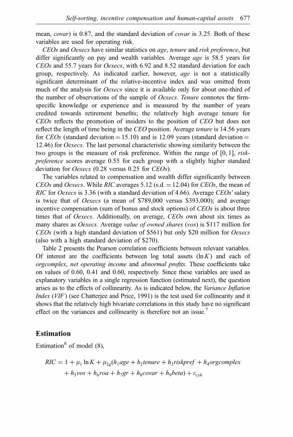
Estimation

Estimation8 of model (8),

RIC ¼ 1 þ m1 lnK þ m2q(h1ageþ h2tenureþ h3riskpref þ h4orgcomplex

þ h5vosþ h6roaþ h7gr þ h8covar þ h9beta) þ ecyh


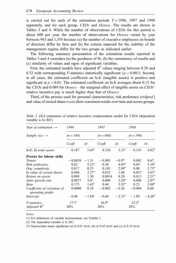
is carried out for each of the estimation periods T¼ 1996, 1997 and 1998

separately, and for each group, CEOs and Oexecs. The results are shown in

Tables 3 and 4. While the number of observations of CEOs for this period is

about 600 per year, the number of observations for Oexecs varied by year

between 965 and 1,354 because (a) the number of executive employees on boards

of directors differ by firm and (b) the criteria imposed for the stability of the

management regime differ for the two groups as indicated earlier.

The following summary presentation of the estimation results reported in

Tables 3 and 4 considers (a) the goodness of fit, (b) the consistency of results and

(c) similarity of values and signs of significant variables.

First, the estimated models have adjusted R2 values ranging between 0.20 and

0.32 with corresponding F-statistics statistically significant (p< 0.001). Second,

in all cases, the estimated coefficient on lnK (tangible assets) is positive and

significant at p< 0.01. The estimated coefficient on lnK averages about 0.15 for

the CEOs and 0.089 for Oexecs – the marginal effect of tangible assets on CEOs’

relative incentive pay is much higher than that of Oexecs.

Third, of the proxies used for personal characteristics, risk preference (riskpref )

and value of owned shares (vos) show consistent results over time and across groups.

Table 3 OLS estimation of relative incentive compensation model for CEOs (dependentvariable is ln RIC)

Year of estimation ! 1996 1997 1998

Sample size ! (n¼ 588) (n¼ 600) (n¼ 590)

Coeff. (t) Coeff. (t) Coeff. (t)

lnK: ln total assets 0.187 5.65a 0.124 3.31a 0.153 4.82a

Proxies for labour skillsTenure �0.0038 �1.31 �0.003 �0.97 0.002 0.67Risk preference 0.62 5.21a 0.58 4.05a 0.69 5.10a

Org. complexity 0.017 0.53 0.103 2.89a 0.08 2.75a

ln value of owned shares 0.044 2.37a 0.022 1.08 0.057 3.63a

Return on assets 0.009 1.30 0.0014 0.20 0.013 2.21a

Sales growth rate 0.0077 3.0a 0.009 3.20a 0.006 2.07a

Beta 0.175 1.65c 0.40 3.52a 0.23 3.09a

Coefficient of variation ofoperating profits

0.0008 0.18 �0.002 �0.26 �0.004 0.60

Intercept �0.48 �1.84c�0.68 �2.31a

�1.09 �4.20a

F-statistics 17.1a 16.9a 23.2a

Adjusted R2 20% 20% 26%

Notes:

(1) For definitions of variable measurement, see Exhibit 1.

(2) The dependent variable is ln RIC.

(3) Superscripts mean significant (a) at 0.01 level, (b) at 0.05 level and (c) at 0.10 level.


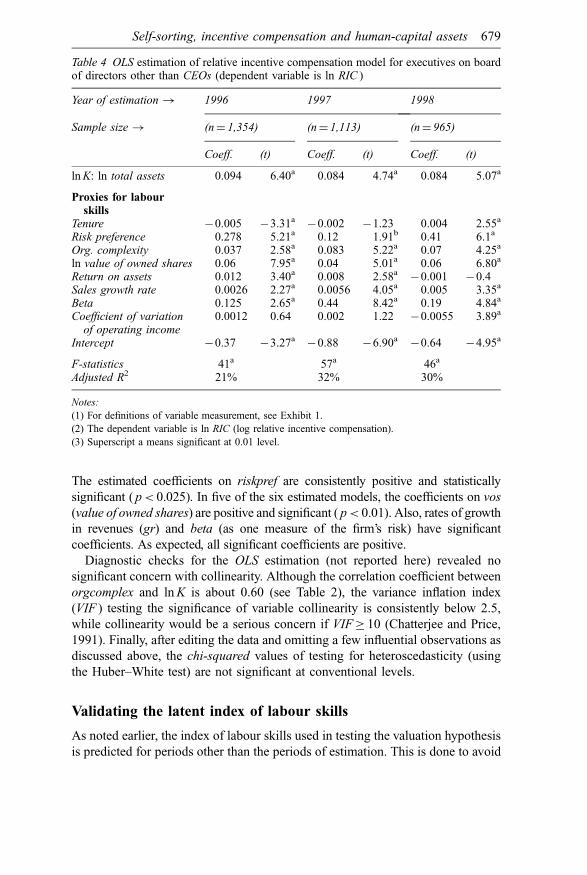
The estimated coefficients on riskpref are consistently positive and statistically

significant ( p< 0.025). In five of the six estimated models, the coefficients on vos

(value of owned shares) are positive and significant ( p< 0.01). Also, rates of growth

in revenues (gr) and beta (as one measure of the firm’s risk) have significant

coefficients. As expected, all significant coefficients are positive.

Diagnostic checks for the OLS estimation (not reported here) revealed no

significant concern with collinearity. Although the correlation coefficient between

orgcomplex and lnK is about 0.60 (see Table 2), the variance inflation index

(VIF ) testing the significance of variable collinearity is consistently below 2.5,

while collinearity would be a serious concern if VIF� 10 (Chatterjee and Price,

1991). Finally, after editing the data and omitting a few influential observations as

discussed above, the chi-squared values of testing for heteroscedasticity (using

the Huber–White test) are not significant at conventional levels.

Validating the latent index of labour skills

As noted earlier, the index of labour skills used in testing the valuation hypothesis

is predicted for periods other than the periods of estimation. This is done to avoid

Table 4 OLS estimation of relative incentive compensation model for executives on boardof directors other than CEOs (dependent variable is ln RIC )

Year of estimation ! 1996 1997 1998

Sample size ! (n¼ 1,354) (n¼ 1,113) (n¼ 965)

Coeff. (t) Coeff. (t) Coeff. (t)

lnK: ln total assets 0.094 6.40a 0.084 4.74a 0.084 5.07a

Proxies for labourskills

Tenure �0.005 �3.31a�0.002 �1.23 0.004 2.55a

Risk preference 0.278 5.21a 0.12 1.91b 0.41 6.1a

Org. complexity 0.037 2.58a 0.083 5.22a 0.07 4.25a

ln value of owned shares 0.06 7.95a 0.04 5.01a 0.06 6.80a

Return on assets 0.012 3.40a 0.008 2.58a�0.001 �0.4

Sales growth rate 0.0026 2.27a 0.0056 4.05a 0.005 3.35a

Beta 0.125 2.65a 0.44 8.42a 0.19 4.84a

Coefficient of variationof operating income

0.0012 0.64 0.002 1.22 �0.0055 3.89a

Intercept �0.37 �3.27a�0.88 �6.90a

�0.64 �4.95a

F-statistics 41a 57a 46a

Adjusted R2 21% 32% 30%

Notes:

(1) For definitions of variable measurement, see Exhibit 1.

(2) The dependent variable is ln RIC (log relative incentive compensation).

(3) Superscript a means significant at 0.01 level.


obtaining results that could be caused by spuriously interpreted relationships.

Spurious relationships would be expected for contemporaneous measures of share

prices and realized index of incentive pay because a large component of the latter

is contingent on the former.

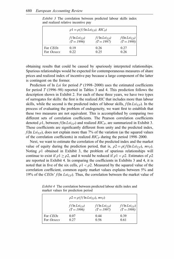
Prediction of ln Lsi for period P (1998–2000) uses the estimated coefficients

for period T (1996–98) reported in Tables 3 and 4. This prediction follows the

description shown in Exhibit 2. For each of these three years, we have two types

of surrogates for skills: the first is the realized RIC that includes more than labour

skills, while the second is the predicted index of labour skills, f (ln LsiT,P). In the

process of evaluating the problem of endogeneity, we want first to establish that

these two measures are not equivalent. This is accomplished by comparing two

different sets of correlation coefficients. The Pearson correlation coefficients

denoted r1, between f (ln LsiT,P) and realized RICP, are summarized in Exhibit 3.

These coefficients are significantly different from unity and the predicted index,

f (ln LsiT,P), does not explain more than 7% of the variation (as the squared values

of the correlation coefficients) in realized RICP during the period 1998–2000.

Next, we want to estimate the correlation of the predicted index and the market

value of equity during the prediction period, that is, r2¼ r( f (ln LsiT,P), mvP).

Noting r1 obtained in Exhibit 3, the problem of spurious relationships will

continue to exist if r1� r2, and it would be reduced if r1< r2. Estimates of r2

are reported in Exhibit 4. In comparing the coefficients in Exhibits 3 and 4, it is

noted that in five of the six cells, r1< r2. Measured by the squared value of the

correlation coefficient, common equity market values explains between 5% and

19% of the CEOs’ f (ln LsiT,P). Thus, the correlation between the market value of

Exhibit 3 The correlation between predicted labour skills indexand realized relative incentive pay

r1¼ r( f ( ln LsiT,P), RICP)

f ( ln LsiT,P)(T¼ 1996)

f ( ln LsiT,P)(T¼ 1997)

f (ln LsiT,P)(T¼ 1998)

For CEOs 0.19 0.26 0.27For Oexecs 0.22 0.25 0.26

Exhibit 4 The correlation between predicted labour skills index andmarket values for prediction period

r2¼ r( f ( ln LsiT,P), mvP)

f ( ln LsiT,P)(T¼ 1996)

f ( ln LsiT,P)(T¼ 1997)

f ( ln LsiT,P)(T¼ 1998)

For CEOs 0.07 0.44 0.39For Oexecs 0.27 0.56 0.61


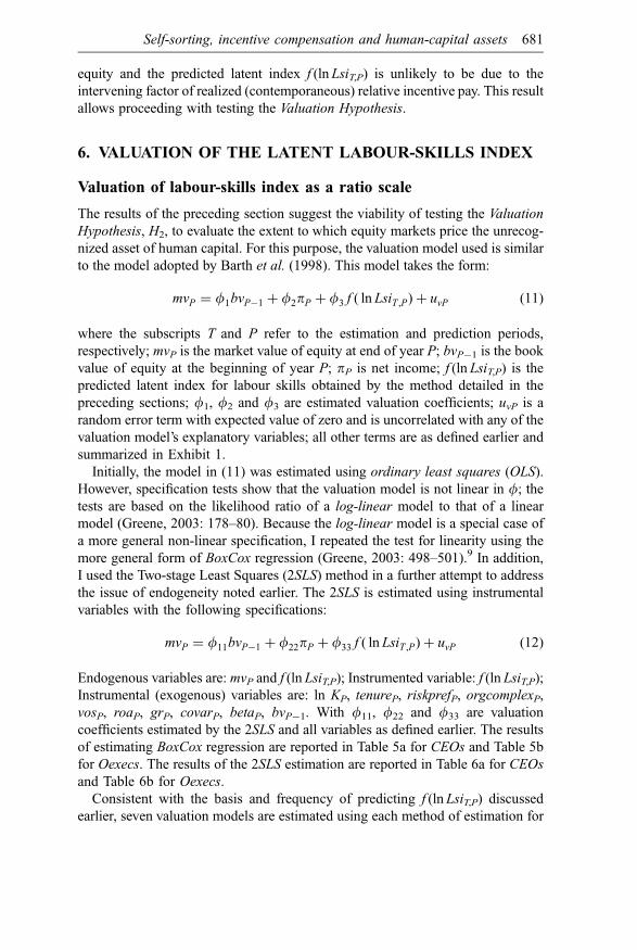
equity and the predicted latent index f (lnLsiT,P) is unlikely to be due to the

intervening factor of realized (contemporaneous) relative incentive pay. This result

allows proceeding with testing the Valuation Hypothesis.

6. VALUATION OF THE LATENT LABOUR-SKILLS INDEX

Valuation of labour-skills index as a ratio scale

The results of the preceding section suggest the viability of testing the Valuation

Hypothesis, H2, to evaluate the extent to which equity markets price the unrecog-

nized asset of human capital. For this purpose, the valuation model used is similar

to the model adopted by Barth et al. (1998). This model takes the form:

mvP ¼ f1bvP�1 þ f2pP þ f3 f ( ln LsiT ,P) þ uvP (11)

where the subscripts T and P refer to the estimation and prediction periods,

respectively; mvP is the market value of equity at end of year P; bvP�1 is the book

value of equity at the beginning of year P; pP is net income; f (ln LsiT,P) is the

predicted latent index for labour skills obtained by the method detailed in the

preceding sections; f1, f2 and f3 are estimated valuation coefficients; uvP is a

random error term with expected value of zero and is uncorrelated with any of the

valuation model’s explanatory variables; all other terms are as defined earlier and

summarized in Exhibit 1.

Initially, the model in (11) was estimated using ordinary least squares (OLS).

However, specification tests show that the valuation model is not linear in f; the

tests are based on the likelihood ratio of a log-linear model to that of a linear

model (Greene, 2003: 178–80). Because the log-linear model is a special case of

a more general non-linear specification, I repeated the test for linearity using the

more general form of BoxCox regression (Greene, 2003: 498–501).9 In addition,

I used the Two-stage Least Squares (2SLS) method in a further attempt to address

the issue of endogeneity noted earlier. The 2SLS is estimated using instrumental

variables with the following specifications:

mvP ¼ f11bvP�1 þ f22pP þ f33 f ( ln LsiT ,P) þ uvP (12)

Endogenous variables are: mvP and f (ln LsiT,P); Instrumented variable: f (ln LsiT,P);

Instrumental (exogenous) variables are: ln KP, tenureP, riskprefP, orgcomplexP,

vosP, roaP, grP, covarP, betaP, bvP�1. With f11, f22 and f33 are valuation

coefficients estimated by the 2SLS and all variables as defined earlier. The results

of estimating BoxCox regression are reported in Table 5a for CEOs and Table 5b

for Oexecs. The results of the 2SLS estimation are reported in Table 6a for CEOs

and Table 6b for Oexecs.

Consistent with the basis and frequency of predicting f (lnLsiT,P) discussed

earlier, seven valuation models are estimated using each method of estimation for


each group: the CEOs and Oexecs. Valuation models are estimated for the

prediction period P¼ 1998, 1999 and 2000 using the predicted values of

f (ln LsiT,P) based on coefficients estimated during T¼ 1996, for period

P¼ 1999 and 2000 using coefficients estimated during T¼ 1997, and for

period P¼ 2000 using coefficients estimated during T¼ 1998.

The results of the BoxCox regressions are significant in rejecting the linearity of

the untransformed model. In all cases, the BoxCox l transformation parameter is

significantly different from 0 (the linear case) and from þ1 (the log-linear case).10

However, the estimated models behave as expected in that (1) the coefficients on

bvP�1 are significantly different from zero (at p< 0.001), and are not significantly

different from unity; (2) the coefficient on net income is positive and significant

(p< 0.01). The results of testing the Valuation Hypothesis (H2) presented in Tables

5a and 5b suggest three properties for the predicted labour skills, f (lnLsiT,P):

(a) the fit-statistics for the models (Wald chi-squared ) are significant

(p< 0.0001);

(b) the coefficients f3 on predicted labour-skills index are positive;

(c) significance levels, as measured by chi-squared for each of the f3

coefficients, are consistently below 0.001; and

(d) the magnitudes of the f3 coefficients do not display any particular pattern

when comparing the coefficients for CEOs versus Oexecs.

Estimating the 2SLS, reported in Tables 6a and 6b, gives results that are very similar

to those obtained using the BoxCox regression. That is, the estimated coefficients

f33 show the same properties as f3. This similarity of the findings using the two

estimation methods suggests that (1) the endogeneity problem is substantially

mitigated, and (2) the Valuation Hypothesis cannot be rejected; i.e. the results are

consistent with H2 – that equity markets appear to value the labour skills of top exe-

cutive teams.

Valuation using the skill index as a dichotomous indicator

In validating the results obtained above, the predicted index of labour skills, f (ln

LsiT,P), is transformed into a binary (dummy indicator) variable, DLsiT,P, where

DLsiT ,P ¼ 1 for high relative labour skills � if f ( ln LsiT ,P) > the mean

DLsiT ,P ¼ 0 for relatively low labour skills � if f ( ln LsiT ,P) � the mean

Replacing f (ln LsiT,P) with the dummy indicator variable DLsiT,P in equations

(11) and (12), I obtain the corresponding regression:

mvP ¼ d1bvP�1 þ d2pP þ d3DLsiT ,P þ uvPd (13)

where d1, d2 and d3 are coefficients, uvPd is an error term N(0, sd), and all other

terms are as defined before. As a parsimonious summary, the results of estimating

(13) are consistent with prior findings of estimating (11) and (12) for both CEOs


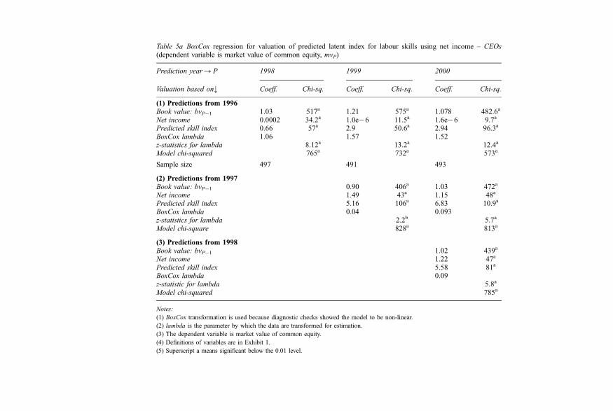
Table 5a BoxCox regression for valuation of predicted latent index for labour skills using net income – CEOs(dependent variable is market value of common equity, mvP)

Prediction year!P 1998 1999 2000

Valuation based on; Coeff. Chi-sq. Coeff. Chi-sq. Coeff. Chi-sq.

(1) Predictions from 1996Book value: bvP�1 1.03 517a 1.21 575a 1.078 482.6a

Net income 0.0002 34.2a 1.0e�6 11.5a 1.6e�6 9.7a

Predicted skill index 0.66 57a 2.9 50.6a 2.94 96.3a

BoxCox lambda 1.06 1.57 1.52z-statistics for lambda 8.12a 13.2a 12.4a

Model chi-squared 765a 732a 573a

Sample size 497 491 493

(2) Predictions from 1997Book value: bvP�1 0.90 406a 1.03 472a

Net income 1.49 43a 1.15 48a

Predicted skill index 5.16 106a 6.83 10.9a

BoxCox lambda 0.04 0.093z-statistics for lambda 2.2b 5.7a

Model chi-square 828a 813a

(3) Predictions from 1998Book value: bvP�1 1.02 439a

Net income 1.22 47a

Predicted skill index 5.58 81a

BoxCox lambda 0.09z-statistic for lambda 5.8a

Model chi-squared 785a

Notes:

(1) BoxCox transformation is used because diagnostic checks showed the model to be non-linear.

(2) lambda is the parameter by which the data are transformed for estimation.

(3) The dependent variable is market value of common equity.

(4) Definitions of variables are in Exhibit 1.

(5) Superscript a means significant below the 0.01 level.

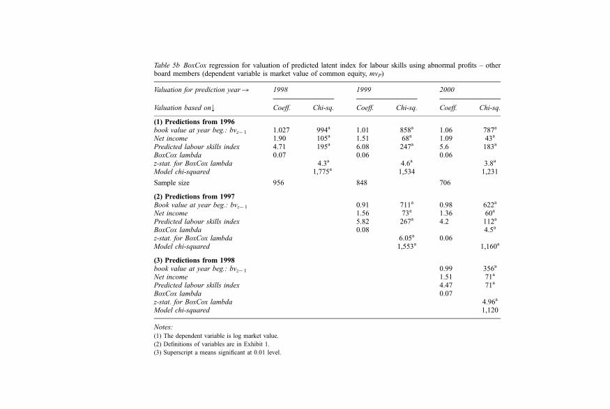
Table 5b BoxCox regression for valuation of predicted latent index for labour skills using abnormal profits – otherboard members (dependent variable is market value of common equity, mvP)

Valuation for prediction year! 1998 1999 2000


(1) Predictions from 1996book value at year beg.: bvz� 1 1.027 994a 1.01 858a 1.06 787a

Net income 1.90 105a 1.51 68a 1.09 43a

Predicted labour skills index 4.71 195a 6.08 247a 5.6 183a

BoxCox lambda 0.07 0.06 0.06z-stat. for BoxCox lambda 4.3a 4.6a 3.8a

Model chi-squared 1,775a 1,534 1,231


(2) Predictions from 1997Book value at year beg.: bvz� 1 0.91 711a 0.98 622a

Net income 1.56 73a 1.36 60a

Predicted labour skills index 5.82 267a 4.2 112a

BoxCox lambda 0.08 4.5a

z-stat. for BoxCox lambda 6.05a 0.06Model chi-squared 1,553a 1,160a

(3) Predictions from 1998book value at year beg.: bvz� 1 0.99 356a

Net income 1.51 71a

Predicted labour skills index 4.47 71a

BoxCox lambda 0.07z-stat. for BoxCox lambda 4.96a

Model chi-squared 1,120

Notes:

(1) The dependent variable is log market value.



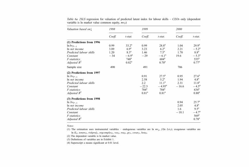
Table 6a 2SLS regression for valuation of predicted latent index for labour skills – CEOs only (dependentvariable is ln market value common equity, mvP)

Valuation based on; 1998 1999 2000

Coeff. t-stat. Coeff. t-stat. Coeff. t-stat.

(1) Predictions from 1996ln bvP�1 0.99 33.2a 0.99 28.8a 1.04 29.9a

ln net income 3.89 6.9a 3.23 6.2a 2.21 �5.2a

Predicted labour skills 1.20 8.3a 1.46 7.5a 1.70 8.8a

Constant �34 �6.9a�29 �6.1a 19.6 �5.3a


Adjusted R2 0.82a 0.70a 0.77a


(2) Predictions from 1997ln bvP�1 0.91 27.5a 0.95 27.6a

ln net income 2.58 5.2a 1.94 4.8a

Predicted labour skills 2.2 11.1a 2.31 11.8a

Constant �22.3 �4.95a�16.6 �4.5a



(3) Predictions from 1998ln bvP�1 0.94 25.7a

ln net income 2.05 4.8a

Predicted labour skills 1.6 9.5a

Constant �18.1 �4.7a

F-statistics 569a

Adjusted R2 0.78a

Notes:

(1) The estimation uses instrumental variables – endogenous variables are ln mvp, f (ln LsiT); exogenous variables are

ln KP, tenureP, riskprefP, orgcomplexP, vosP, roaP, grP, covarP, betaP.

(2) The dependent variable is ln market value.



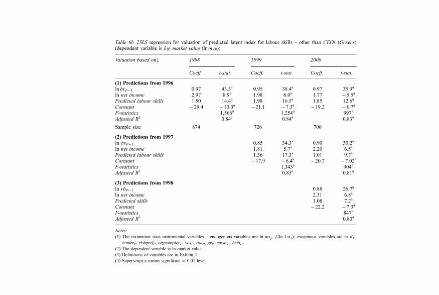
Table 6b 2SLS regression for valuation of predicted latent index for labour skills – other than CEOs (Oexecs)(dependent variable is log market value (lnmvP))

Valuation based on; 1998 1999 2000

Coeff. t-stat. Coeff. t-stat. Coeff. t-stat.

(1) Predictions from 1996ln bvP�1 0.97 43.3a 0.95 38.4a 0.97 35.9a

ln net income 2.97 8.9a 1.98 6.0a 1.77 �5.5a

Predicted labour skills 1.50 14.4a 1.98 16.5a 1.85 12.6a

Constant �29.4 �10.0a�21.1 �7.3a

�19.2 �6.7a

F-statistics 1,566a 1,254a 997a



(2) Predictions from 1997ln bvP�1 0.85 34.3a 0.90 30.2a

ln net income 1.81 5.7a 2.20 6.5a

Predicted labour skills 1.36 17.3a 1.01 9.7a

Constant �17.9 �6.4a�20.7 �7.02a

F-statistics 1,343a 904a

Adjusted R2 0.85a 0.81a

(3) Predictions from 1998ln vbP�1 0.88 26.7a

ln net income 2.31 6.8a

Predicted skills 1.08 7.2a

Constant �22.2 �7.3a

F-statistics 847a

Adjusted R2 0.80a

Notes:

(1) The estimation uses instrumental variables – endogenous variables are ln mvp, f (ln LsiT); exogenous variables are ln KP,

tenureP, riskprefP, orgcomplexP, vosP, roaP, grP, covarP, betaP.

(2) The dependent variable is ln market value.



and Oexecs. The BoxCox estimation results for the CEOs are presented in Table 7a

and the 2SLS are presented in Table 7b. The results are consistent with those

using f (ln Lsi) as a ratio scale. The list of properties reported above for both f3

and f33 are repeated here for d3; the only difference is in the magnitude of the

coefficients on the DLsiT,P as compared to those obtained for f (ln LsiT,P), which is

the result of changing scale. Thus, the Valuation Hypothesis (H2) cannot be

rejected whether using ratio or a binary scale for the predicted latent index of

human capital.

7. EFFECT OF INDUSTRY TYPE

Different types of managerial skills are suited for different industries, which

create segmentation in labour markets. For example, the managers hired by public

utilities (electric, water, gas, etc.) do not, in general, search for positions with

technology firms or financial institutions. The term ‘public’ used in reference to

this industry is descriptive of the type of goods or services provided; it does not

connote the type of ownership because the majority of public utility firms are (at

least in the United States) privately owned and their equity shares are traded on

stock exchanges. Thus, these firms have the same contracting and incentive

problems as other firms. Unlike many other competitive industries, however,

public utilities in the United States generate their revenues, to a great extent, as a

function of the cost structure of their operations. This is the result of cost-plus

pricing regulations and of dependence on large government subsidies when

market forces fail (e.g. the recent case in the state of California). To the designers

of the system, this is a fair exchange: public utilities guarantee continuous supply

of service (e.g. electricity) and, in exchange, they are protected from competition

and are guaranteed a fair rate of return.

It can, therefore, be argued that top executives of those firms would be more

useful to their shareholders if they were skilful negotiators who could extract

higher rates from the state public service commissions (see, for example, Abdel-

khalik, 1988a; Lanen and Larcker, 1992). As a result, the challenge for top

executives to compete for selling the output of their firms in the marketplace is

limited. In contrast, technology firms operate in a highly competitive environment

in which barriers to entry are very low and risk is very high. Consequently,

managing innovation, developing new products and entering new markets is

crucial to the success of executives employed in the technology sector. This

means that the abilities, talents and institutional knowledge required for managing

companies in these two sectors differ considerably. This difference is manifested

in different degrees of risk sharing and pay for performance (i.e. relative incentive

pay) for these two sectors.

It is therefore plausible that the findings in this study do not apply to certain

types of industries. To illustrate these differences, consider the summary results

in Table 8. This table shows the means of variables related to CEO compensation

during the period 1998–2000 for a selected group of industries in comparison with


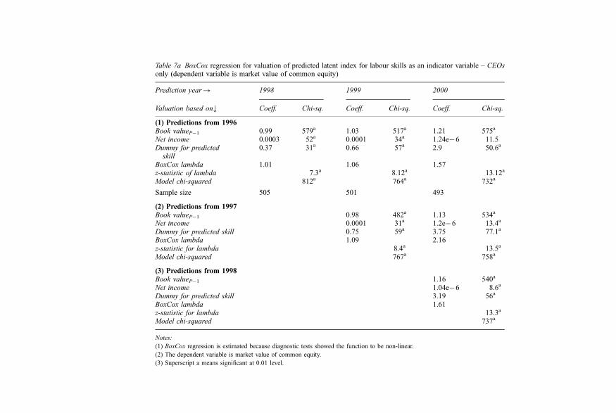
Table 7a BoxCox regression for valuation of predicted latent index for labour skills as an indicator variable – CEOsonly (dependent variable is market value of common equity)

Prediction year! 1998 1999 2000


(1) Predictions from 1996Book valueP�1 0.99 579a 1.03 517a 1.21 575a

Net income 0.0003 52a 0.0001 34a 1.24e�6 11.5Dummy for predictedskill

0.37 31a 0.66 57a 2.9 50.6a

BoxCox lambda 1.01 1.06 1.57z-statistic of lambda 7.3a 8.12a 13.12a

Model chi-squared 812a 764a 732a


(2) Predictions from 1997Book valueP�1 0.98 482a 1.13 534a

Net income 0.0001 31a 1.2e�6 13.4a

Dummy for predicted skill 0.75 59a 3.75 77.1a

BoxCox lambda 1.09 2.16z-statistic for lambda 8.4a 13.5a

Model chi-squared 767a 758a

(3) Predictions from 1998Book valueP�1 1.16 540a

Net income 1.04e�6 8.6a

Dummy for predicted skill 3.19 56a

BoxCox lambda 1.61z-statistic for lambda 13.3a

Model chi-squared 737a

Notes:

(1) BoxCox regression is estimated because diagnostic tests showed the function to be non-linear.

(2) The dependent variable is market value of common equity.


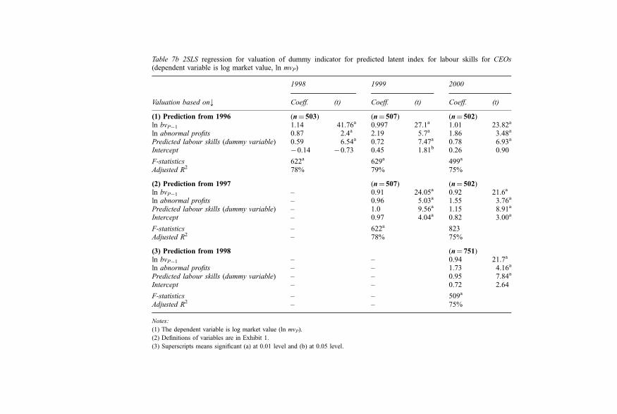
Table 7b 2SLS regression for valuation of dummy indicator for predicted latent index for labour skills for CEOs(dependent variable is log market value, ln mvP)

1998 1999 2000

Valuation based on; Coeff. (t) Coeff. (t) Coeff. (t)

(1) Prediction from 1996 (n¼ 503) (n¼ 507) (n¼ 502)ln bvP�1 1.14 41.76a 0.997 27.1a 1.01 23.82a

ln abnormal profits 0.87 2.4a 2.19 5.7a 1.86 3.48a

Predicted labour skills (dummy variable) 0.59 6.54a 0.72 7.47a 0.78 6.93a

Intercept �0.14 �0.73 0.45 1.81b 0.26 0.90


Adjusted R2 78% 79% 75%

(2) Prediction from 1997 (n¼ 507) (n¼ 502)ln bvP�1 – 0.91 24.05a 0.92 21.6a

ln abnormal profits – 0.96 5.03a 1.55 3.76a

Predicted labour skills (dummy variable) – 1.0 9.56a 1.15 8.91a

Intercept – 0.97 4.04a 0.82 3.00a

F-statistics – 622a 823Adjusted R2 – 78% 75%

(3) Prediction from 1998 (n¼ 751)ln bvP�1 – – 0.94 21.7a

ln abnormal profits – – 1.73 4.16a

Predicted labour skills (dummy variable) – – 0.95 7.84a

Intercept – – 0.72 2.64

F-statistics – – 509a

Adjusted R2 – – 75%

Notes:

(1) The dependent variable is log market value (ln mvP).


(3) Superscripts means significant (a) at 0.01 level and (b) at 0.05 level.

the total sample. The industrial classification used is that of Standard & Poor’s

Industry Classification Index, which groups firms by the core businesses in which

they operate. Seven industrial groups are presented in Table 8: foods, healthcare,

oil and gas, financial institutions, manufacturing, computer and information

technology, and public utilities.

It is clear from Table 8 that the index of relative incentive compensation (RIC )

varies widely across different industries. Average RIC ranges from 2.85 for public

utilities to 10.34 for computers and information technology. In terms of the

magnitude of RIC, financial institutions and healthcare industries are next in rank

to computers and information technology. Inspection of detailed compensation

components shows that the primary source of difference is not in the annual

salary as much as it is in the value of stock options and annual bonuses. The sum

of the latter two items average annually about $9 million for CEOs in computer

and information technology and $1.6 million for CEOs in public utilities.

The empirical analysis of valuation of the predicted latent index of managerial

skills was replicated for these different industry groups. The results show that the

Valuation Hypothesis H2 holds well for various industrial classifications, except

for healthcare (classification 35), oil and gas (classification 40) and public utilities

(classification 90). While this finding suggests the relevance of the unique

features of different industries, it also suggests the need for further study of

the institutional and market arrangements that cause these differences, which is

the subject for another study.

8. ADDITIONAL ROBUSTNESS TESTS

Two types of robustness checks are carried out: the first is for the sample choice,

and the second is for the valuation model. The data structure is a panel of cross-

section=time-series observations. Because of serial dependency, pooling the data

for analysis leads to understating the estimation errors as well as other estimation

problems. For this reason, the preceding analysis is carried out year-by-year. In

checking the reproducibility of this analysis, I replicated the results using random

sampling. This replication is made for CEOs, Oexecs and the combined set. For

each group, two sub-samples are selected at random from: an estimation sub-

sample (equivalent to T in the preceding analysis) representing 15% of the data

set, and a prediction sub-sample (corresponding to P in the preceding analysis)

consisting of 30% of the total number of observations. This led to six random

samples, two for each grouping. The results of these random samples confirm

those obtained earlier for year-by-year analysis.11

9. SUMMARY

The aim of this study is to find a viable surrogate for human capital, which is

defined as the skills embodied in employees, as it relates to the employer’s assets.

In the age of technology and information, human assets have become the primary


Table 8 A summary of average CEO compensation for different industries (1998–2000)

SPINDEX(a) All 30 35 40 50 60 80 90Industry All Foods Health-

careOil & gas Finance Mnfg Computers &

info. tech.Publicutilities

Sample size(no. of firms) 512 31 32 34 63 78 27 51

RIC* 5.70 6.73 7.57 6.90 8.14 4.35 10.34 2.85Salary** 739 798 898 729 775 724 786 624Bonus** 948 1,441 882 824 1,794 873 1,268 493Long-termincentive pay**

350 203 536 516 470 497 309 367

Stock optionsNumber 218 278 334 300 223 165 103 237Black & Scholesvalue**

3,552 4,755 6,320 2,785 3,938 1,090 7,716 1,376

Value of sharesowned***

104 242 83 31 309 269 33 10

Notes:

(a) The two-digit Standard & Poor Industry Classification Index.

*Ratio of relative incentive compensation per dollar of salary.

**In thousand dollars.

***In million dollars.

source of adding value to their employer firms. As an intangible, however,

investments in human resources are neither measured nor reported. As with any

other asset, the value of human capital to the firm might be viewed as the present

value of future income to the firm emanating from investment in human

resources, and the research question of interest is whether capital markets

recognize and value this asset even when accounting does not.

Concurrent with the information revolution is the increase in the proportion of

at-risk compensation; incentive pay and stock-based compensation have become

mainstays in the modern corporation, especially in North America. In this study,

relative incentive pay per dollar of salary is used to estimate a proxy for the extent

to which a firm values its management team. The basic motivation draws on the

self-sorting framework in labour economics: the more-skilled managers will

choose to work for firms that reward them more for employing their skills. That

type of manager would seek higher expected compensation based on performance

instead of accepting a guaranteed, but lower fixed pay. The literature in labour

economics has shown that informed labour markets exhibit this self-sorting

feature.

Accepting the definition of human capital as the skills embodied in people,

I propose that relative incentive pay in a Cobb–Douglas world depends on two

types of capital: human capital and tangible productive assets. For empirical

analysis, I assume that labour skills depend on personal variables (experience,

risk aversion and value of owned shares) and proxies for the ability to manage

(return on assets, revenue growth rate, organizational complexity and operating

risk). Along with relative incentive pay and tangible capital, these variables are

used to estimate and forecast a latent index for labour skills. To determine the

extent to which labour markets recognize and value the intangible assets that

are not reported by the accounting system, the predicted latent index is included

in an equity valuation model.

The data used for empirical analysis are obtained from ExecuComp and other

public data sources. The analysis is carried out for the period 1996–2000 for a

sample of about 600 firms. Imputed labour skills indices are predicted for CEOs,

Oexecs members of the board and for a combined set of both groups. The

empirical estimation uses OLS, BoxCox regression and 2SLS. The Valuation

Hypothesis tested using the valuation model of Barth–Beaver–Landsman (with

book values of equity, net income and omitted variables as determining price).

The omitted variable in this case is the predicted latent index for labour skills

measured as (a) a ratio scale or (b) a dichotomous indicator variable.

The contribution of this study lies in substantiating the feasibility of using

relative incentive compensation (incentive pay per dollar of fixed salary) as a

surrogate for human capital. The basic results are based on (a) developing a latent

index for labour skills as a derivative of relative incentive pay, and (b) validating

that index using capital market valuation of unrecognized assets. The findings of

this study are consistent throughout the analysis using both ratio and dummy

indicator scales.


Further analysis, however, shows that the results do not hold for some

industries (e.g. public utilities), which is an issue that extends beyond the

scope of this study and is left for a future project.

ACKNOWLEDGEMENTS

Special thanks go to Ira Horowitz and two anonymous reviewers for making

valuable comments on an earlier draft of the paper. Numerous helpful comments

were received from Bipin Ajinkya, Sasson Bar-Yosef, Allen Blay, Sanjeev

Bhojraj, Keejae Hong, Adel Ibrahim, Ken Koga, Avi Kohl, Sri Ramamoorti,

Theodore Sougiannis, Shyam Sunder, Hong Xie, David Ziebart, and workshop

participants at the University of Florida, Florida State University, the University

of Kansas, the University of Illinois at Urbana-Champaign, the University of

Illinois at Chicago, and the Hong Kong University of Science and Technology.

Earlier drafts of this paper were also presented at the Fourth European Conference

on Capital Markets, Cyprus, October 2002; the Big-Ten Faculty Research

Consortium held at the University of Iowa in June 2001; the European Account-

ing Congress held in Munich, Germany, in May 2000; and the Third Conference

on Corporate Governance at the Chinese University of Hong Kong in 1999. Also

special thanks go to the Editors of this Special Issue on Intangibles, Baruch Lev

and Stefano Zambon.

NOTES

1 The Cobb–Douglas production function was developed for macro (aggregated) data,although much of the literature has used this form for micro-data. Simon (1979)discusses the biases of estimating a Cobb–Douglas function and suggests that thehomogeneity of the function is a statistical artefact. However, I use this form in thisstudy as a starting point to develop an empirical model for relative incentive pay.

2 The concept of relative incentive compensation might be illustrated by two celebratedreal-life cases with each attempting to use the equivalent of RIC to induce executives toreveal their talents. The first is the case of Lee Iacoca at the Chrysler Corporation. Inthe 1980s he accepted a one-dollar annual salary and stacked all his expectedcompensation on stock options, a calculated decision that later earned him millionsof dollars in stock-option awards. The second case is that of Michael Eisner at Disney.His first contract (Crystal, 1990: 354) consisted of the following components: a basesalary of $750,000 a year; 2% of profits in excess of a 9% ROE (rate of return onequity) level; and an option on about 2 million common shares at a strike price of$14.00 a share with a ten-year exercise period. In his fourth year, Eisner earned anannual bonus of $7 million and the value of his options reached $104 million (Crystal,1990: 355).

3 Tangible assets are used as measures of physical capital. The accounting measures ofassets, however, are measured by mixed attributes containing historical cost, currentcost and estimated present values.

4 The deferral of exercising vested and in-the-money options may be viewed asproviding a joint signal of risk taking and expectations of future profitability. In thispaper, I use only the former. The latter implication is the subject of another study.


5 This analysis is replicated using random samples for the estimation and predictionperiods T and P.

6 I had expected that the risk preference scores would differ between the CEOs andOexecs. However, the data do not bear out this expectation. Examination of this issue isdeferred for a future study.

7 I used STATA in all the empirical analyses reported in this study. The preferred test forcollinearity is based on the degree to which the variance is inflated due to thecollinearity of variables. This index is discussed in Chatterjee and Price (1991). Iused STATA for all the analyses.

8 It would be desirable to estimate the coefficients m1 and m2q for each firm separately.However, a long time series is required for estimation of firm-specific parameters. Thecross-section analysis, therefore, is only a representation of average results.

9 The reason for using the log-transformation to begin with in the previous drafts is dueto the non-linearity of the models used in Barth et al. (1998) and others. Testing fornon-linearity is based on the likelihood ratio of estimating models under differentspecifications. For example, consider the BoxCox regression:

mvP ¼ a0bv(l)P�1 þ a3 f (ln Lsi

(l)T ,P) þ e

where for any of the explanatory variables, say it is x, the transformed value x(l) ismeasured by x(l)

¼ (xl7 1)=l; if l¼ 1, the model is linear, and if l¼ 0, the model islog-linear; otherwise, the model is non-linear of a different form.

To illustrate the test carried out in this paper, a comparison for the valuation modelfor P¼ 1999 using the predictions based on T¼ 1996 is shown below:

Linearcoefficient (t)

Log-linearcoefficient (t)

BoxCoxcoefficient (w2)

a0 2.09 (6.14) 0.99 (28.6) 0.99 (490)a1 17.52 (12.82) 3.33 (6.4) 1.53 (49)a3 69.72 (1.92) 1.25 (7.7) 1.63 (37)

Adjusted R2 0.72 0.79 –Model w2 – – 843Model F-statistic 4.24 607 –

Likelihood ratio test of l¼ 0, w2¼ 3.6 ( p¼ 0.058); l¼ 1, w2

¼ 2,317 ( p¼ 0) (seeGreene, 2003; all estimation and tests are carried out using STATA).

10 The BoxCox transformation requires that all variables be greater than zero. To satisfythis property, I added a constant to each variable. Adding a constant does not alter theresults of estimation.

11 The tables presenting the results of the random samples are available from the authoron request.

REFERENCES

Abdel-khalik, A. R. (1988a) ‘Incentives for accruing costs and efficiency in regulatedmonopolies subject to ROE constraint’, Journal of Accounting Research, 26 (Supple-ment): 144–81.

Abdel-khalik, A. R. (1988b) ‘Hierarchies and size: a problem of identification’, Organiza-tion Studies, 9(2): 237–51.


Aboody, D. and Lev, B. (1998) ‘The value relevance of intangibles: the case of softwarecapitalization’, Journal of Accounting Research, 36 (Supplement): 161–91.

Albert, S. and Bradley, K. (1997) Managing Knowledge: Experts, Agencies and Organiza-tions. New York: Cambridge University Press.

Amir, E. and Livne, G. (2002) ‘Accounting for human capital when labour mobility isrestricted’, Working Paper, Tel Aviv University.

Bahk, B.-H. and Gort, M. (1993) ‘Decomposing learning by doing in new plants’, Journalof Political Economy, 101(4): 561–83.

Barth, M. E., Beaver, W. H. and Landsman, W. R. (1998) ‘Relative valuation roles ofequity book value and net income as a function of financial health’, Journal ofAccounting and Economics, 25: 1–34.

Becker, G. (1964) Human Capital. New York: Columbia University Press.Bresnahan, T. F., Brynjolfsson, E. and Lorin, M. H. (2002) ‘Information technology,

workplace organization, and the demand for skilled labor: firm level evidence’,Quarterly Journal of Economics, 67(1): 339–76.

Brown, C. and Medoff, J. (1989) ‘The employer size–wage effect’, Journal of PoliticalEconomy, 97(5): 1027–59.

Brummet, L. L., Flamholtz, E. and Pyle, W. (1968) ‘Human resource measurement –a challenge for accountants’, Accounting Review, 66 (April): 217–30.

Caplan, E. H. and Landekich, S. (1973) Human Resource Accounting: Past, Present andFuture. New York: National Association of Accountants.

Chatterjee, S. and Price, B. (1991) Regression Analysis by Example, 2nd edn. New York:John Wiley.

Crystal, G. S. (1990) ‘CEO compensation: the case of Michael Eisner’, in ExecutiveCompensation: A Strategic Guide for the 1990s. Boston, MA: Harvard Business SchoolPress, pp. 335–65.

Dittman, D. A., Juris, H. A. and Revsine, L. (1976) ‘On the existence of unrecognisedhuman assets: an economic perspective’, Journal of Accounting Research, 14 (Spring):49–65.

Doms, M., Dunne, T. and Troske, K. R. (1997) ‘Workers, wages and technology’,Quarterly Journal of Economics, 62(1): 253–90.

Donkers, B., Melenberg, B. and Van Soest, A. (2001) ‘Estimating risk attitudes usinglotteries: a large sample approach’, Journal of Risk and Uncertainty, 22(2): 165–95.

Edvinsson, L. and Malone, M. (1997) Intellectual Capital. New York: Harper.Elias, N. (1972) ‘The effects of human asset statements on the investment decision: an

experiment’, Journal of Accounting Research, 10 (Supplement): 215–33.Financial Accounting Standards Board (1995) Accounting for Stock-Based Compensation,

Statement of Financial Accounting Standards No. 123. Norwalk, CT: FinancialAccounting Standards Board.

Flamholtz, E. (1969) ‘The theory and measurement of an individual’s value to anorganization’, unpublished Ph.D. dissertation, University of Michigan, Ann Arbor.

Flamholtz, E. (1971) ‘A model for human resource valuation: a stochastic process withservice rewards’, Accounting Review, 46 (April): 253–67.

Flamholtz, E. (1999) Human Resource Accounting, 3rd edn. Boston, MA: KluwerAcademic.

Friedman, A. and Lev, B. (1974) ‘A surrogate measure for the firm’s investment in humancapital’, Journal of Accounting Research, 12(2): 235–50.

Greene, W. H. (2003) Econometric Analysis, 5th edn. New York: Macmillan.Griliches, Z. and Mason, W. M. (1972) ‘Education, income and ability’, Journal of

Political Economy, 80(3) Part 2: S74–S103.Groshen, E. (1991) ‘The structure of female=male differential: is it who you are, what you

do, or where you work?’, Journal of Human Resources, 26 (Summer): 457–72.


Guay, W. R. (1999) ‘The sensitivity of CEO wealth to equity risk: an analysis of themagnitude and determinants’, Journal of Financial Economics, 53: 43–71.

Hansson, B. (2001) ‘Human capital and stock returns: is the value premium anapproximation for return on human capital?’, SSRN Electronic Paper Collection.

Hartog, J., Ferrer-I-Carbonell, A. and Jonker, N. (2000) ‘On a simple survey measure ofindividual risk aversion’, Working Paper No. 363, CESifo, Germany, and WorkingPaper, University of Amsterdam.

Hvide, H. K. and Kaplan, T. (2003) ‘Delegated job design’, Working Paper, NorwegianSchool of Economics and Business.

Jagannathan, R., Keiichi, K. and Hitoshi, T. (1998) ‘Relationship between labour-incomerisk and average return: empirical evidence from the Japanese stock markets’, Journal ofBusiness, 71 (July): 319–47.

Jovanovic, B. (1979) ‘Job matching and the theory of turnover’, Journal of PoliticalEconomy, 87: 972–90.

Lanen, W. N. and Larcker, D. (1992) ‘Executive compensation contract adoption in theelectric utility industry’, Journal of Accounting Research, 30(1): 70–93.

Lazear, E. P. (1986) ‘Salaries and piece rates’, Journal of Business, 59 (July): 405–31.Lazear, E. P. (1998) Personnel Economics for Managers. New York: John Wiley.Lazear, E. P. (2000) ‘Performance pay and productivity’, American Economic Review, 90:

1346–61.Lev, B. (2001) Intangibles: Management, Measurement, and Reporting. Washington, DC:

Brookings Institution.Lev, B. and Schwartz, A. (1971) ‘On the use of the economic concept of human capital in

financial statement’, Accounting Review, 26(1): 103–12.Likert, R. and Bowers, D. G. (1973) ‘Improving the accuracy of P=L reports by estimating the

change in dollar value of the human organization’, Michigan Business Review, 25: 15–24.Likert, R. and Pyle, W. C. (1971) ‘A human organizational measurement approach’,

Financial Analysts Journal, January–February: 75–84.Loehman, E. (1998) ‘Testing risk aversion and nonexpected utility theories’, Journal

of Economic Behavior and Organization, 33: 285–302.MacDonald, G. M. (1980) ‘Person-specific information in the labour market’, Journal

of Political Economy, 88(3): 578–97.Maddala, G. S. (1988) Introduction to Econometrics, 2nd edn. New York: Macmillan.Mincer, J. (1962) ‘On-the-job-training: costs, returns, and some implications’, Journal

of Political Economy, 70: 50–79.Mincer, J. (1974) Schooling, Experience and Earnings. New York: National Bureau

of Economic Research.Morse, W. J. (1973) ‘A note on the relationship between human assets and human capital’,

Accounting Review, 48: 589–93.Mouritsen, J., Larsen, H. T. and Bukh, P. N. D. (2001) ‘Intellectual capital and the ‘‘capable

firm’’: narrating, visualizing and numbering for managing knowledge’, Accounting,Organizations and Society, 26: 735–62.

Petty, R. and Guthrie, J. (2000) ‘Intellectual capital literature review: measurement,reporting and management’, Journal of Intellectual Capital, 1(2): 155–76.

Raviv, A. (1985) ‘Management compensation and the managerial labour market: anoverview’, Journal of Accounting and Economics, 7 (April): 239–46.

Rogers, D. A. (2002) ‘Does executive portfolio structure affect risk management? CEOrisk incentives and corporate derivatives usage’, Journal of Banking and Finance,36: 271–95.

Rosett, J. (2001) ‘Equity risk and the labour stock: the case of union contracts’, Journal ofAccounting Research, 39(2): 337–64.


Sackman, S. A., Flamholtz, E. G. and Bullen, M. L. (1985) ‘Human resource accounting:a state-of-the-art review’, Journal of Accounting Literature, 8: 235–64.

Schooley, D. K. and Worden, D. D. (1996) ‘Risk aversion measures: comparing attitudesand asset allocations’, Financial Services Review, 5(2): 87–99.

Schultz, T. W. (1961) ‘Investment in human capital’, American Economic Review, 51: 1–17.Simon, H. A. (1979) ‘On the parsimonious explanations of the production relations’,

Scandinavian Journal of Economics, 81: 459–474. Reproduced in Models of BoundedRationality (1982) Vol. 1. Cambridge, MA: MIT Press, pp. 444–59.

Sougiannis, T. (1994) ‘The accounting based valuation of corporate R&D’, AccountingReview, 69 (January): 26–43.

Teulings, C. (1995) ‘The wage distribution in a model of the assignment of skills to jobs’,Journal of Political Economy, 103(2): 280–315.

Topel, R. H. (2000) ‘Managing the workplace’, Lecture Notes for Topic 1: Labour marketsand human capital. Lecture Notes for Business 343, University of Chicago GraduateSchool of Business.


Copyright of European Accounting Review is the property of Routledge and its content may not be copied or

emailed to multiple sites or posted to a listserv without the copyright holder's express written permission.

However, users may print, download, or email articles for individual use.

Documents

Self-sorting, incentive compensation and human-capital · PDF fileSelf-sorting, incentive compensation and ... Not estimating a value for human capital and not recognizing it ... incentive