Embed Size (px)
Citation preview
CAS/CNS TR-2009-006 Self-Supervised ARTMAP 1
Self-Supervised ARTMAP
Gregory P. Amis and Gail A. Carpenter
Department of Cognitive and Neural Systems Boston University 677 Beacon Street
Boston, MA, 02215
[gamis, gail] @cns.bu.edu
May, 2009
Neural Networks, in press.
Technical Report CAS/CNS TR-2009-006 Boston, MA: Boston University
Acknowledgements: This research was supported by the SyNAPSE program of the Defense Advanced Projects Research Agency (Hewlett-Packard Company, subcontract under DARPA prime contract HR0011-09-3-0001, and HRL Laboratories LLC, subcontract #801881-BS under DARPA prime contract HR0011-09-C-0001) and by CELEST, an NSF Science of Learning Center (SBE-0354378).
CAS/CNS TR-2009-006 Self-Supervised ARTMAP 2
Self-Supervised ARTMAP
Abstract: Computational models of learning typically train on labeled input patterns (supervised learning), unlabeled input patterns (unsupervised learning), or a combination of the two (semi-supervised learning). In each case input patterns have a fixed number of features throughout training and testing. Human and machine learning contexts present additional opportunities for expanding incomplete knowledge from formal training, via self-directed learning that incorporates features not previously experienced. This article defines a new self-supervised learning paradigm to address these richer learning contexts, introducing a neural network called self-supervised ARTMAP. Self-supervised learning integrates knowledge from a teacher (labeled patterns with some features), knowledge from the environment (unlabeled patterns with more features), and knowledge from internal model activation (self-labeled patterns). Self-supervised ARTMAP learns about novel features from unlabeled patterns without destroying partial knowledge previously acquired from labeled patterns. A category selection function bases system predictions on known features, and distributed network activation scales unlabeled learning to prediction confidence. Slow distributed learning on unlabeled patterns focuses on novel features and confident predictions, defining classification boundaries that were ambiguous in the labeled patterns. Self-supervised ARTMAP improves test accuracy on illustrative low-dimensional problems and on high-dimensional benchmarks. Model code and benchmark data are available from: http://techlab.bu.edu/SSART/. Keywords: Self-supervised learning, supervised learning, Adaptive Resonance Theory (ART), ARTMAP, unsupervised learning, machine learning 1. Supervised, unsupervised, semi-supervised, and self-supervised learning Computational models of supervised pattern recognition typically utilize two learning phases. During an initial training phase, input patterns, described as values of a fixed set of features, are presented along with output class labels or patterns. During a subsequent testing phase, the model generates output predictions for unlabeled inputs, while no further learning takes place. Although the supervised learning paradigm has been successfully applied for a wide variety of applications, it does not reflect many natural learning situations. Humans do learn from explicit training, as from a textbook or a teacher, and they do take tests. However, students do not stop learning when they leave the classroom. Rather, they continue to learn from experience, incorporating not only more information but new types of information, all the while building on their earlier classroom knowledge. The self-supervised learning system introduced here models such life-long experiences. An unsupervised learning system clusters unlabeled input patterns. Semi-supervised systems (Chapelle, Schölkopf, & Zien, 2006) learn from unlabeled as well as labeled inputs during training. The self-supervised paradigm models two learning stages. During Stage 1 learning, the system receives all output labels, but only a subset of possible feature values for each input. During Stage 2 learning, the system receives all feature values for each input, but no output

CAS/CNS TR-2009-006 Self-Supervised ARTMAP 3
labels (Table 1).
Table 1
Learning paradigms
Paradigm
Learning
Training set
No learning
Test set
Input features Output labels
Supervised All All All input
features
________
All output
labels
Semi-supervised Stage 1 All All
Stage 2 All None
Self-supervised
New definition
Stage 1 Some All
Stage 2 All None
Unsupervised All None
Preparing students for a lifetime of independent learning has always been a primary principle of good education. As described by Stephen Krashen, an expert in second language acquisition:
An autonomous acquirer is not a perfect speaker of the second language, just good enough to continue to improve without us. This is, of course, the goal of all education – not to produce masters but to allow people to begin work in their profession and to continue to grow. (Krashen, 2004, p. 6)
Self-supervised learning models the continuing growth of the autonomous acquirer. By analogy with Stage 1 learning, a medical student may, for example, initially learn to treat diseases from case studies with clear diagnoses for a small sample of patients using a limited number of specified features such as major symptoms and test results. Later in practice (Stage 2), the doctor, no longer supervised, diagnoses patients with myriad symptoms, test results, and contexts that were not fully specified during training. The doctor not only successfully treats under these enhanced circumstances but also learns from the experiences. In addition to modeling the human learning experience, self-supervised learning promises to be useful for technological applications such as web page classification. A supervised learning system that completes all training before making test predictions does not adapt to new information and varying contexts. An adaptive system that continues to learn unsupervised during testing risks degrading its supervised knowledge. The self-supervised learning system
CAS/CNS TR-2009-006 Self-Supervised ARTMAP 4
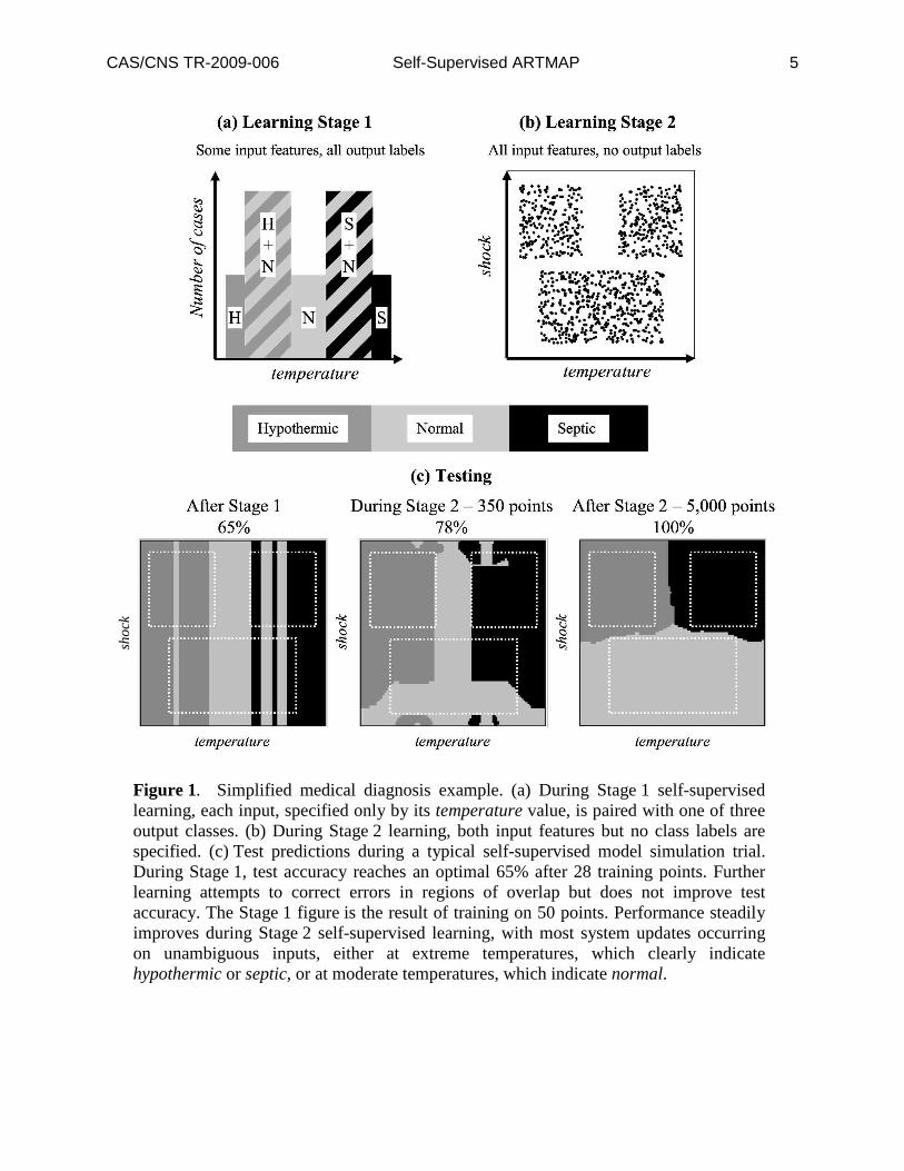
developed here continues to learn from new experiences without, in most cases, degrading performance. 2. A computational example of self-supervised learning A simplified medical diagnosis example
(Figure 1) illustrates the dynamics of the self-supervised
learning model. The problem is to identify exemplars as belonging to the output class normal or hypothermic or septic, given the input feature values temperature and shock. During Stage 1 learning, class labels are paired with inputs that specify only the feature temperature (Figure 1a). The system models incremental online learning that addresses just one case at a time. Projected onto the temperature axis, classes overlap, and, even with a large training set, optimal test accuracy is 65%. Although extreme temperatures unambiguously indicate hypothermic or septic, these class labels are densely mixed with normal at moderately low and moderately high temperatures. During Stage 2 self-supervised learning, inputs specify both temperature and shock, but no class labels are provided (Figure 1b). The self-supervised learning system has an opportunity to incorporate shock information, but needs to be designed in such a way that it does not degrade the partial knowledge that it gained during Stage 1 learning. Figure 1c illustrates results of a typical self-supervised learning simulation. Following Stage 1, where only one input feature (temperature) was available, the model attains a near-optimal test accuracy of 65%. During slow self-supervised Stage 2 learning on unlabeled (but fully featured) inputs, the model adds novel shock information to Stage 1 temperature knowledge. After 5,000 Stage 2 learning samples, the test set is labeled with 100% accuracy. 3. ART and ARTMAP The self-supervised learning system of Figure 1 is based on Adaptive Resonance Theory (ART). ART neural networks model real-time prediction, search, learning, and recognition. Design principles derived from scientific analyses and design constraints imposed by targeted applications have jointly guided the development of many variants of the basic supervised learning ARTMAP networks, including fuzzy ARTMAP (Carpenter, Grossberg, Markuzon, Reynolds, & Rosen, 1992), ARTMAP-IC (Carpenter & Markuzon, 1998), and Gaussian ARTMAP (Williamson, 1998). A defining characteristic of various ARTMAP systems is the nature of their internal code representations. Early ARTMAP networks, including fuzzy ARTMAP, employed winner-take-all coding, whereby each input activates a single category node during both training and testing. When a node is first activated during training, it is mapped to its designated output class.
CAS/CNS TR-2009-006 Self-Supervised ARTMAP 5
sho
ck
Figure 1. Simplified medical diagnosis example. (a) During Stage 1 self-supervised learning, each input, specified only by its temperature value, is paired with one of three output classes. (b) During Stage 2 learning, both input features but no class labels are specified. (c) Test predictions during a typical self-supervised model simulation trial. During Stage 1, test accuracy reaches an optimal 65% after 28 training points. Further learning attempts to correct errors in regions of overlap but does not improve test accuracy. The Stage 1 figure is the result of training on 50 points. Performance steadily improves during Stage 2 self-supervised learning, with most system updates occurring on unambiguous inputs, either at extreme temperatures, which clearly indicate hypothermic or septic, or at moderate temperatures, which indicate normal.
CAS/CNS TR-2009-006 Self-Supervised ARTMAP 6
Starting with ART-EMAP (Carpenter & Ross, 1995), ARTMAP systems have used distributed coding during testing, which typically improves predictive accuracy while avoiding the computational challenges inherent in the use of distributed code representations during training. In order meet these challenges, distributed ARTMAP (Carpenter, 1997; Carpenter, Milenova, & Noeske, 1998) introduces a new network configuration and new learning laws that realize stable fast learning with distributed coding during both training and testing. Comparative analysis of the performance of ARTMAP systems on a variety of benchmark problems has led to the identification of a default ARTMAP network (Carpenter, 2003; Amis & Carpenter, 2007), which features simplicity of design and robust performance in many application domains (http://techlab.bu.edu/). Default ARTMAP employs winner-take-all coding during training and distributed coding during testing within a distributed ARTMAP network architecture. During Stage 1, when the system can incorporate externally specified output labels with confidence, self-supervised ARTMAP (SS ARTMAP) employs winner-take-all coding and fast learning. During Stage 2, when the network internally generates its own output labels, codes are distributed and learning is slow, so that incorrect hypotheses do not abruptly override Stage 1 “classroom learning.” Sections 3.1 – 3.4 introduce the key ARTMAP computations that are implemented in the SS ARTMAP architecture. 3.1. Complement coding: Learning both absent and present features Unsupervised ART and supervised ARTMAP networks employ a preprocessing step called complement coding (Carpenter, Grossberg, & Rosen, 1991). When the learning system is presented with a set of input features a ≡ a1...ai ...aM( ), complement coding doubles the number
of input components, presenting to the network both the original feature vector and its complement. Complement coding allows a learning system to encode features that are consistently absent on an equal basis with features that are consistently present. Features that are sometimes absent and sometimes present when a given category is being learned become regarded as uninformative with respect to that category. To implement complement coding, component activities ia of an M-dimensional feature vector a
are scaled so that 0 1ia≤ ≤ . For each feature i, the ON activity a
i( ) determines the
complementary OFF activity ( )1 ia− . Both a and its complement ac are concatenated to form
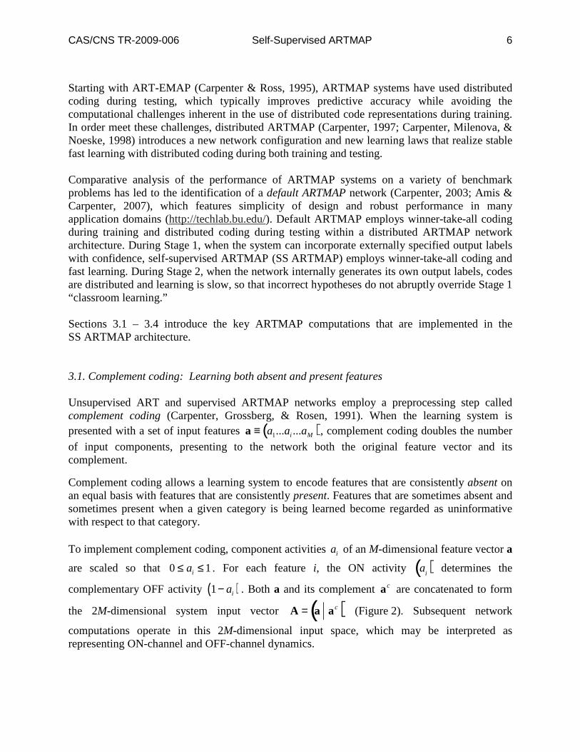
the 2M-dimensional system input vector A = a ac( ) (Figure 2). Subsequent network
computations operate in this 2M-dimensional input space, which may be interpreted as representing ON-channel and OFF-channel dynamics.
CAS/CNS TR-2009-006 Self-Supervised ARTMAP 7
Figure 2. Complement coding transforms an M-dimensional feature vector a into a 2M-dimensional system input vector A. A complement-coded system input represents both the degree to which a feature i is present ai( ) and the degree to which that feature is
absent 1− ai( ).
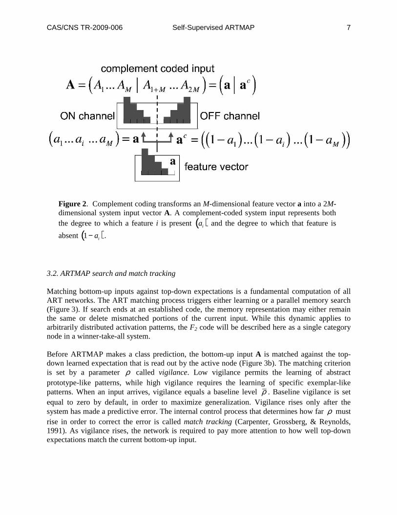
3.2. ARTMAP search and match tracking Matching bottom-up inputs against top-down expectations is a fundamental computation of all ART networks. The ART matching process triggers either learning or a parallel memory search (Figure 3). If search ends at an established code, the memory representation may either remain the same or delete mismatched portions of the current input. While this dynamic applies to arbitrarily distributed activation patterns, the F2 code will be described here as a single category node in a winner-take-all system. Before ARTMAP makes a class prediction, the bottom-up input A is matched against the top-down learned expectation that is read out by the active node (Figure 3b). The matching criterion is set by a parameter ρ called vigilance. Low vigilance permits the learning of abstract prototype-like patterns, while high vigilance requires the learning of specific exemplar-like patterns. When an input arrives, vigilance equals a baseline level ρ . Baseline vigilance is set equal to zero by default, in order to maximize generalization. Vigilance rises only after the system has made a predictive error. The internal control process that determines how far ρ must rise in order to correct the error is called match tracking (Carpenter, Grossberg, & Reynolds, 1991). As vigilance rises, the network is required to pay more attention to how well top-down expectations match the current bottom-up input.
CAS/CNS TR-2009-006 Self-Supervised ARTMAP 8
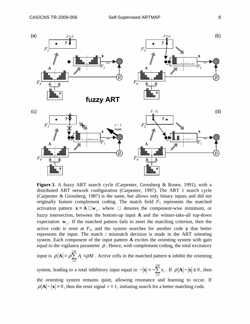
Figure 3. A fuzzy ART search cycle (Carpenter, Grossberg & Rosen, 1991), with a distributed ART network configuration (Carpenter, 1997). The ART 1 search cycle (Carpenter & Grossberg, 1987) is the same, but allows only binary inputs and did not originally feature complement coding. The match field F1 represents the matched activation pattern x = A ∧ w
J, where ∧ denotes the component-wise minimum, or
fuzzy intersection, between the bottom-up input A and the winner-take-all top-down expectation wJ
. If the matched pattern fails to meet the matching criterion, then the
active code is reset at F2, and the system searches for another code y that better represents the input. The match / mismatch decision is made in the ART orienting system. Each component of the input pattern A excites the orienting system with gain equal to the vigilance parameter ρ . Hence, with complement coding, the total excitatory
input is 2
1
M
ii
A Mρ ρ ρ=
= =∑A . Active cells in the matched pattern x inhibit the orienting
system, leading to a total inhibitory input equal to 2
1
M
ii
x=
− = −∑x . If 0ρ − ≤A x , then
the orienting system remains quiet, allowing resonance and learning to occur. If 0ρ − >A x , then the reset signal r = 1, initiating search for a better matching code.
CAS/CNS TR-2009-006 Self-Supervised ARTMAP 9
Match tracking forces an ARTMAP system not only to reset its mistakes, but to learn from them. With match tracking and fast learning, each ARTMAP network passes the Next Input Test, which requires that, if a training input were re-presented immediately after its learning trial, it would directly activate the correct output class, with neither predictive errors nor search. While match tracking guarantees that a winner-take-all network passes the Next Input Test, it does not also guarantee that a distributed prediction, such as those made during default ARTMAP testing, would pass the Next Input Test. A training step added to default ARTMAP 2 does provide such a guarantee (Amis & Carpenter, 2007). Match tracking simultaneously implements the design goals of maximizing generalization and minimizing predictive error, without requiring the choice of a fixed matching criterion. ARTMAP memories thereby include both broad and specific pattern classes, with the latter formed as exceptions to the more general “rules” defined by the former. ARTMAP learning typically produces a wide variety of such mixtures, whose exact composition depends upon the order of training exemplar presentation. Activity x at the ART field F1 continuously computes the match between the field’s bottom-up and top-down input patterns. The reset signal r shuts off the active F2 node J when x fails to meet the matching criterion determined by the value of the vigilance parameter ρ . Reset alone does not, however, trigger a search for a different F2 node: unless the prior activation has left an enduring trace within the F0-to-F2 subsystem, the network will simply reactivate the same node as before. As modeled in ART 3 (Carpenter & Grossberg, 1990), biasing the bottom-up input to the coding field F2 to favor previously inactive nodes implements search by allowing the network to activate a new node in response to a reset signal. The ART 3 search mechanism defines a medium-term memory in the F0-to-F2 adaptive filter which biases the system against rechoosing a node that had just produced a reset. 3.3. Committed nodes and uncommitted nodes With winner-take-all ARTMAP fast learning, a node J becomes committed the first time it is activated. The weight vector wJ converges to the input A, and node J is permanently linked to the current output. Unless they have already activated all their coding nodes, ART systems contain a reserve of nodes that have never been activated, with weights at their initial values. These uncommitted nodes receive bottom-up inputs and compete on an equal footing with the previously activated nodes. Any input may then choose an uncommitted node over poorly matched committed nodes (Figure 4).
CAS/CNS TR-2009-006 Self-Supervised ARTMAP 10
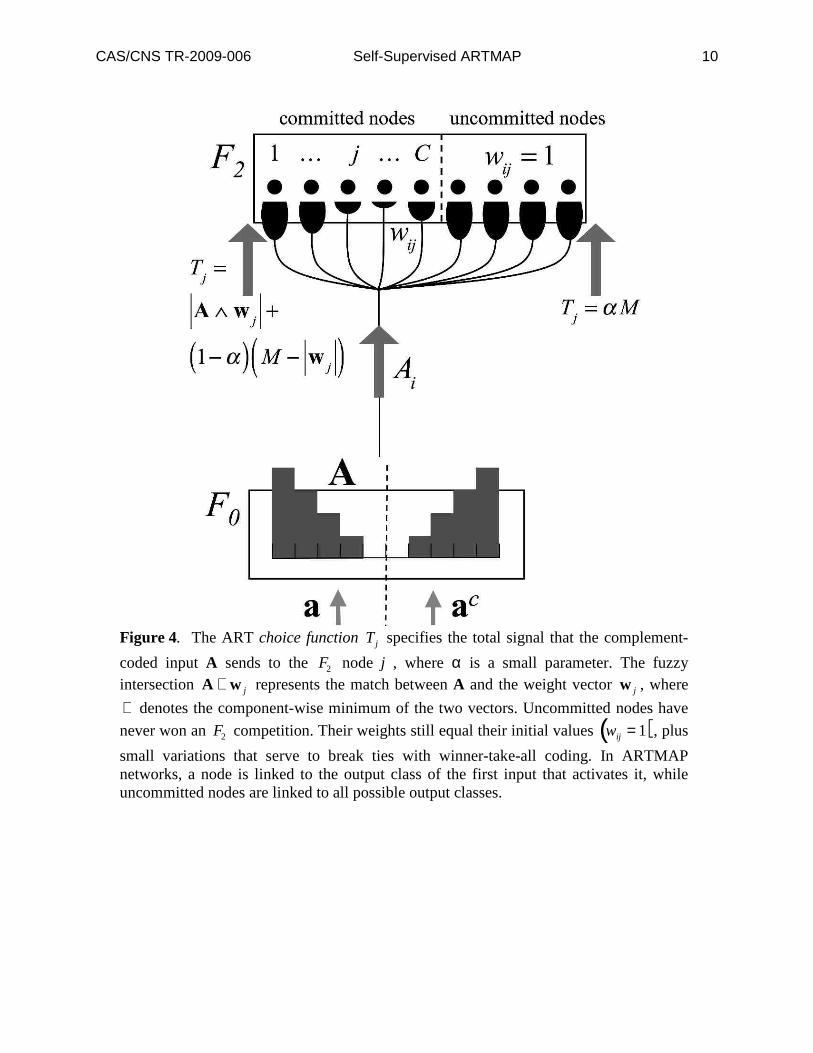
Figure 4. The ART choice function Tj specifies the total signal that the complement-
coded input A sends to the F2 node j , where α is a small parameter. The fuzzy intersection A ∧ w j represents the match between A and the weight vector w j , where
∧ denotes the component-wise minimum of the two vectors. Uncommitted nodes have
never won an F2 competition. Their weights still equal their initial values wij = 1( ), plus
small variations that serve to break ties with winner-take-all coding. In ARTMAP networks, a node is linked to the output class of the first input that activates it, while uncommitted nodes are linked to all possible output classes.
CAS/CNS TR-2009-006 Self-Supervised ARTMAP 11
An ARTMAP design constraint specifies that an active uncommitted node should not reset itself. Weights begin with all wij = 1 . Since 0 ≤ Ai ≤ 1, when a winner-take-all active node J is
uncommitted, match field activity x = A ∧ wJ = A . In this case, therefore,
ρ A − x = ρ A − A = ρ − 1( ) A . Thus ρ A − x ≤ 0 and an uncommitted node does not
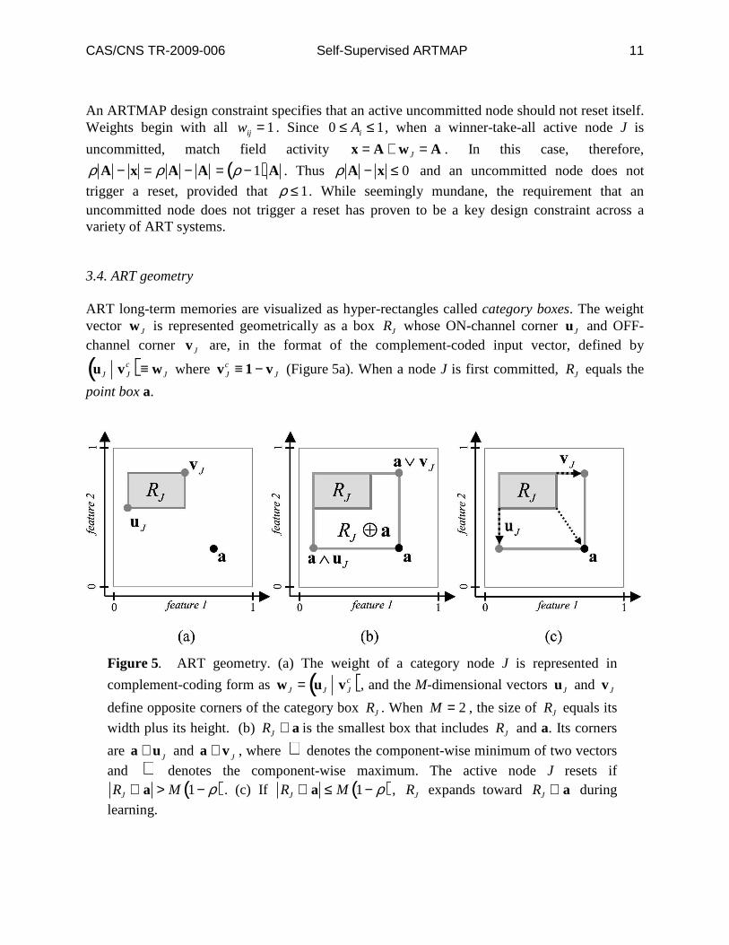
trigger a reset, provided that ρ ≤ 1. While seemingly mundane, the requirement that an uncommitted node does not trigger a reset has proven to be a key design constraint across a variety of ART systems. 3.4. ART geometry ART long-term memories are visualized as hyper-rectangles called category boxes. The weight vector wJ is represented geometrically as a box RJ whose ON-channel corner uJ and OFF-channel corner vJ are, in the format of the complement-coded input vector, defined by
uJ v Jc( )≡ wJ where v J
c ≡ 1 − v J (Figure 5a). When a node J is first committed, RJ equals the
point box a.
Figure 5. ART geometry. (a) The weight of a category node J is represented in
complement-coding form as wJ = uJ v Jc( ), and the M-dimensional vectors uJ and vJ
define opposite corners of the category box RJ . When M = 2 , the size of RJ equals its
width plus its height. (b) JR ⊕ a is the smallest box that includes JR and a. Its corners
are a ∧ uJ and a ∨ v
J, where ∧ denotes the component-wise minimum of two vectors
and ∨ denotes the component-wise maximum. The active node J resets if RJ ⊕ a > M 1− ρ( ). (c) If RJ ⊕ a ≤ M 1− ρ( ), RJ expands toward RJ ⊕ a during
learning.
CAS/CNS TR-2009-006 Self-Supervised ARTMAP 12
For fuzzy ART, the choice-by-difference F0 → F2 signal function (Figure 4) is defined as:
Tj = A ∧ w j + 1− α( ) M − w j( ) (1)
(Carpenter & Gjaja, 1994). The function Tj translates to a geometric interpretation of category
choice. The size Rj of box j is defined as the sum of the edge lengths vij − uij( )i =1
M
∑ , which
implies that
Rj = M − w j .
Rj ⊕ a , defined as the smallest box enclosing both Rj and a (Figure 5b), has size:
Rj ⊕ a = M − A ∧ w j ,
and the city-block (L1 ) distance from Rj to a is:
d Rj ,a( )= Rj ⊕ a − Rj = w j − A ∧ w j .
Thus geometrically the choice function is:
Tj = M − d Rj ,a( )− α Rj . (2)
When the choice parameter α is small, maximizing Tj is almost equivalent to minimizing
d Rj ,a( ), so an input a activates the node J of the closest category box RJ . In case of a distance
tie, as when a lies in more than one box, the node with the smallest Rj is chosen.
According to the ART vigilance matching criterion, the chosen node J will reset if: ρ A − A ∧ wJ = ρM − A ∧ wJ > 0 ,
or, geometrically, if: RJ ⊕ a > M 1− ρ( ).
If node J is not reset, RJ expands toward RJ ⊕ a during learning (Figure 5c). Vigilance thereby sets an upper bound on the size of RJ , with
RJ ≤ M 1− ρ( )≤ M 1− ρ( ).
After a fast learning trial, RJnew = RJ
old ⊕ a .
4. Self-supervised ARTMAP: Geometry
ART weights w
ij initially equal 1. With winner-take-all coding, while the category node J is
active yJ = 1( ), bottom-up weights in F0→ F
2 paths decrease during learning according to a
version of the instar (Grossberg, 1976) learning law:
Instar
d
dtw
iJ= y
Jx
i− w
iJ( )= Ai∧ w
iJ− w
iJ( )= − wiJ
− Ai
+
= − wiJ
− Ai( ) if w
iJ> A
i
0 otherwise
. (3)
CAS/CNS TR-2009-006 Self-Supervised ARTMAP 13
In equation (3), i = 1...2M and ...[ ]+ denotes rectification, with p[ ]+ ≡ max p,0{ }. Top-down
weights w
ji obey an outstar (Grossberg, 1968) learning law, but with fast learning,
w
ji= w
ij.
Recall that, for i = 1...M , Ai
= ai and
w
ij= u
ij. Thus by (3), while node J is active, uiJ
values
decrease during learning according to:
d
dtu
iJ= − u
iJ− a
i
+= − u
iJ− a
i( ) if uiJ
> ai
0 otherwise
.
Geometrically, uJ moves toward a, subject to the constraints of rectification (Figure 6a).
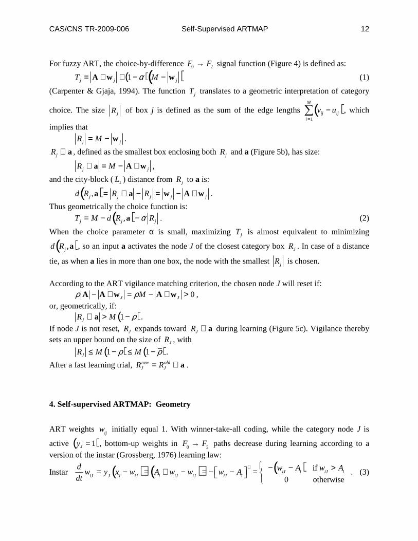
Figure 6. Geometry of ART learning. (a) During learning, components of the category box corner uJ
can only decrease. (b) Similarly, components of the corner v J can only
increase during learning.
Also for i = 1...M , A
i + M= 1− a
i( ) and w
i + M , j= 1− v
ij( ). Thus while the category node J is
active, viJ values increase during learning according to:
d
dtv
iJ= a
i− v
iJ
+= a
i− v
iJ( ) if viJ
< ai
0 otherwise
.
Like uJ, v J
moves toward a, subject to the constraints of rectification (Figure 6b).
With winner-take-all coding and fast learning, weights converge to their asymptotes on each input trial. In this case, J →w A when node J is first activated, and J →u a and J →v a .
Thereafter, node J is committed. On subsequent learning trials that activate J (without reset), RJ
expands just enough to incorporate input a (Figure 5c).
CAS/CNS TR-2009-006 Self-Supervised ARTMAP 14
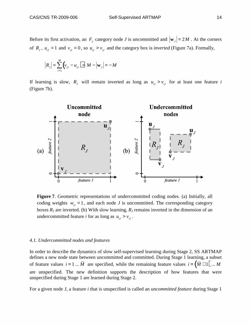
Before its first activation, an F2 category node J is uncommitted and
w
J= 2M . At the corners
of RJ, uiJ
= 1 and viJ= 0 , so uiJ
> viJ
and the category box is inverted (Figure 7a). Formally,
R
J= v
iJ− u
iJ( )i =1
M
∑ = M − wJ
= − M
If learning is slow, RJ
will remain inverted as long as uiJ> v
iJ for at least one feature i
(Figure 7b).
Figure 7. Geometric representations of undercommitted coding nodes. (a) Initially, all coding weights wiJ
= 1, and each node J is uncommitted. The corresponding category
boxes RJ are inverted. (b) With slow learning, RJ remains inverted in the dimension of an undercommitted feature i for as long as uiJ
> viJ
.
4.1. Undercommitted nodes and features In order to describe the dynamics of slow self-supervised learning during Stage 2, SS ARTMAP defines a new node state between uncommitted and committed. During Stage 1 learning, a subset
of feature values i = 1 ... M are specified, while the remaining feature values i = M + 1( ) ... M
are unspecified. The new definition supports the description of how features that were unspecified during Stage 1 are learned during Stage 2. For a given node J, a feature i that is unspecified is called an uncommitted feature during Stage 1
CAS/CNS TR-2009-006 Self-Supervised ARTMAP 15
learning. Whether or not a feature is specified, all weights obey the same learning law. By equation (3), the self-supervised learning model hypothesis that weights maintain their initial values at uncommitted features is equivalent to the hypothesis that Ai
= Ai + M
= 1 for the
unspecified features i = M + 1( ) ... M . Note that during Stage 1 learning A is complement coded
only for the specified features i = 1 ... M , and that A = M + 2 M − M( )= 2M − M .
At the start of Stage 2 SS ARTMAP learning, all uiJ
= 1 and viJ= 0 for features
i = M + 1( ) ... M . With slow learning, these features do not immediately become fully
committed, which requires that uiJ≤ v
iJ (Figure 5). For as long as iJ iJu v> , i is said to be an
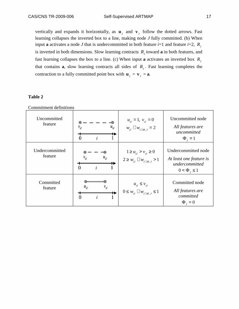
undercommitted feature with respect to node J, and node J is said to be an undercommitted node if its weight vector has one or more undercommitted features. Figure 8 illustrates the geometry of Stage 2 learning at undercommitted nodes. Table 2 summarizes the definitions of feature commitment levels. The degree of feature undercommitment, defined as
Φ
iJ= u
iJ− v
iJ
+,
quantifies the amount of learning needed for node J to become fully committed in feature i. The average
Φ
J= 1
MΦ
iJi =1
M
∑
quantifies the degree of undercommitment of node J.
CAS/CNS TR-2009-006 Self-Supervised ARTMAP 16
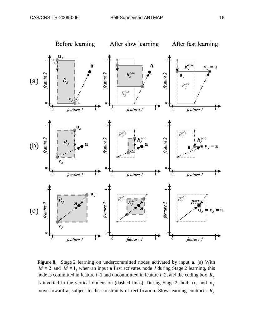
Figure 8. Stage 2 learning on undercommitted nodes activated by input a. (a) With M = 2 and M = 1, when an input a first activates node J during Stage 2 learning, this node is committed in feature i=1 and uncommitted in feature i=2, and the coding box RJ
is inverted in the vertical dimension (dashed lines). During Stage 2, both uJ and v J
move toward a, subject to the constraints of rectification. Slow learning contracts RJ
CAS/CNS TR-2009-006 Self-Supervised ARTMAP 17
vertically and expands it horizontally, as uJ and v J
follow the dotted arrows. Fast
learning collapses the inverted box to a line, making node J fully committed. (b) When input a activates a node J that is undercommitted in both feature i=1 and feature i=2, RJ
is inverted in both dimensions. Slow learning contracts RJtoward a in both features, and
fast learning collapses the box to a line. (c) When input a activates an inverted box RJ
that contains a, slow learning contracts all sides of RJ. Fast learning completes the
contraction to a fully committed point box with uJ = v J
= a.
Table 2
Commitment definitions
Uncommitted feature
uiJ
= 1, viJ
= 0
wiJ
+ wi + M ,J
= 2
Uncommitted node
All features are uncommitted
ΦJ= 1
Undercommitted
feature
1≥ uiJ
> viJ
≥ 0
2 ≥ wiJ
+ wi + M ,J
> 1
Undercommitted node
At least one feature is undercommitted
0 < ΦJ
≤ 1
Committed
feature
uiJ
≤ viJ
0 ≤ wiJ
+ wi + M ,J
≤ 1
Committed node
All features are committed
ΦJ= 0
CAS/CNS TR-2009-006 Self-Supervised ARTMAP 18
Recall that w
J≡ u
J,v
Jc( ), so:
Φ
J= 1
Mw
iJ− w
i + M ,Jc
+
i =1
M
∑ =
1M
wiJ
+ wi + M ,J
− 1
+
i =1
M
∑ . (4)
For an uncommitted node, all wiJ= 1 and ΦJ
= 1. For a committed node, all uiJ≤ v
iJ and
ΦJ= 0 . Once a node J has been activated during Stage 1, features i = 1...M are committed
u
iJ≤ v
iJ( ) while features i = M + 1...M remain uncommitted u
iJ= 1, v
iJ= 0( ), so
Φ
J= M − M( ) M .
5. Distributed Stage 2 learning SS ARTMAP Stage 2 learning updates weights according to the learning laws of distributed ART architectures (Carpenter, 1997). 5.1. Distributed ART learning Distributed ART networks are designed to support stable fast learning with arbitrarily distributed
F2 code patterns y. Achieving this computational goal led to the definition of a new unit of
memory, a dynamic weight
y j − τ ij
+ equal to the degree to which the activity of coding node j
exceeds an adaptive threshold τ ij . The distributed instar (dInstar) updates the thresholds
τ ij in
bottom-up pathways from F0 to
F2 , and the distributed outstar (dOutstar) updates thresholds
τ ji in top-down pathways from
F2 to
F1 :
dInstar (bottom-up):
d
dtτ ij = y j − τ ij
+− Ai
+
= y j − τ ij − Ai
+ (5)
dOutstar (top-down):
d
dtτ ji = y j − τ ji
+σ i − xi( ) , where
σ i = yλ − τλi
+
λ∑ (6)
In the dOutstar equation (6), the top-down dynamic weight
y j − τ ji
+ is proportional to the
input from the F2 node j to the
F1 node i, and
σ i is the total input from
F2 to node i (Carpenter,
1994). During dOutstar learning, the top-down signal σ i tracks
F1 activity
xi , with each
adaptive threshold τ ji increasing according to the contribution of its dynamic weight to the total
signal, with fast as well as slow learning. Formally defining the bottom-up weights
wij ≡ 1− τ ij and the top-down weights
wji ≡ 1− τ ji
CAS/CNS TR-2009-006 Self-Supervised ARTMAP 19
transforms equations (5) and (6) to:
dInstar (bottom-up):
d
dtwij = − y j − 1− wij( )− Ai
+
dOutstar (top-down):
d
dtwji = − y j − 1− wji( )
+σ i − xi( ) , where
σ i = yλ − 1− wλi( )
+
λ∑
With winner-take-all coding,
y j =
1 if j = J
0 if j ≠ J
In this case, the bottom-up dynamic weight is
y j − τ ij
+=
1− τ iJ( ) if j = J
0 if j ≠ J
=
wiJ if j = J
0 if j ≠ J
.
With winner-take-all fast learning, bottom-up and top-down weights are equal. In this case, with
xi = Ai ∧ wiJ when node j=J is active, dInstar and dOutstar equations reduce to an instar learning
law (equation (3)). Even with fast learning, bottom-up weights of distributed ART do not generally equal top-down weights. This is because, according to distributed instar learning , a bottom-up weight
wij
depends only on the activity y j at its target node. In contrast, according to distributed outstar
learning, a top-down weight wji is a function of the entire active coding pattern y.
SS ARTMAP employs winner-take-all fast learning during Stage 1. Therefore at the start of Stage 2, bottom-up weights equal top-down weights. During Stage 2 learning, the
F2 code y is
distributed, so bottom-up and top-down weights would diverge. Since top-down weights will not be used again, they are not computed in the current SS ARTMAP algorithm. Extensions of this system that alternate between Stage 1 and Stage 2 learning, or that need to compute the bottom-up/top-down match during Stage 2 or testing, would need to update the top-down weights via distributed outstar learning during Stage 2. The dInstar and dOutstar equations are piecewise-linear and can be solved analytically. During Stage 2 learning, weights are updated according to the dInstar solution:
wij = wij
old − β y j − 1− wijold( )− Ai
+
where 0 < β ≤ 1. With fast learning, β = 1. With slow learning, β is small. Simulations here set
β = 0.01 for Stage 2 slow learning computations.
CAS/CNS TR-2009-006 Self-Supervised ARTMAP 20
5.2. Distributed activation patterns During SS ARTMAP testing and Stage 2 learning, the
F2 code is distributed, with the activation
pattern y a contrast-enhanced and normalized version of the F0 → F2 signal pattern T. While the
transformation of T to y is assumed to be realized in a real-time network by a competitive field, simulations typically approximate competitive dynamics in their steady-state, according to an algebraic rule. For this purpose, the SS ARTMAP algorithm uses the Increased Gradient Content-Addressable Memory (IG CAM) Rule, which was developed for distributed ARTMAP (Carpenter et al., 1998). The IG CAM Rule features a contrast parameter p. As p increases, the T → y transformation becomes increasingly sharp, approaching winner-take-all as p → ∞ . SS ARTMAP simulations set p=2 for distributed activation during Stage 2 and testing. The hypothesis that SS ARTMAP activation is winner-take-all during Stage 1 learning, when answers are provided, corresponds to the hypothesis that confidence modulates the competitive field, with high-confidence states corresponding to large values of the contrast parameter p. With the IG CAM Rule, if a is in one or more category boxes, activation
y j is distributed among
these nodes, with y j largest where the boxes
Rj that contain a are smallest. If a is not in any
box, y j is distributed according to the distance
d Rj ,a( ), with
y j largest where a is closest to
Rj .
6. Modifying the choice function for undercommitted coding nodes During Stage 2, when learning is slow and distributed and inputs a are fully featured, the degree
of undercommitment Φ
j decreases from
1− M M( ) toward 0 as a coding node j gradually
becomes more committed. Within Stage 2, Φ
jvalues vary across nodes. The ART choice
function T
j as defined by equation (1) would favor more committed nodes to the point that
nodes that became active early in Stage 2 would block learning in all other nodes. Self-supervised ARTMAP therefore modifies the definition of
T
j so that the less committed nodes
are able to compete successfully with the more committed nodes, as follows. 6.1. Balancing committed and undercommitted nodes during Stage 2 learning Fast-learn winner-take-all ARTMAP networks choose the coding node J that maximizes the choice-by-difference signal function:
CAS/CNS TR-2009-006 Self-Supervised ARTMAP 21
T
j= M − w
j− A ∧ w
j( )− α M − wj( ) =
M − d R
j,a( )− α R
j
(Figure 4). Since α is small, the choice function T
j favors nodes j whose category boxes
R
j are
closest to a. Distance ties are broken in favor of smaller boxes. The example illustrated in Figure 9 shows that, in a learning system with mixed degrees of coding node commitment, this signal function also implicitly favors the nodes with greatest commitment. In order to focus on primary
T
j design with respect to the distance from
R
j to a, α is temporarily set equal to 0:
T
j≅
M − d R
j,a( ). (7)
Figure 9 illustrates a hypothetical case such as might occur during Stage 2 self-supervised learning, when various coding nodes j have different degrees of undercommitment
Φ
j
(equation (4)). In this example, node j=1 is fully committed Φ
1= 0( ), while node j=2 is still
uncommitted in feature i=2
Φ2
= 0.5( ). If the ARTMAP choice function (equation (7)) were
used, the signal T1 to the committed node j=1 would be greater than the signal T2
to the
undercommitted node j=2 for all inputs a, as indicated by the grey area of Figure 9a. This function excessively favors nodes that happened to become active, and therefore more committed, early in Stage 2. Many of the Stage 1 nodes would be left permanently inactive, unable either to contribute to predictions or to learn from Stage 2 experience. To see why the signal function of Figure 9a favors committed over undercommitted nodes, note that, for any a at the start of Stage 2, all weights
w
ij= w
i + M , j= 1 for features i = M + 1...M .
Thus at this moment,
d R
j,a( )≡ w
j− A ∧ w
j= w
ij− A
i
+
i =1
2M
∑ =
wij
− ai
++ w
i + M , j− 1− a
i( )
+
i =1
M
∑ =
wij
− ai
++ w
i + M , j− 1− a
i( )
+
i =1
M
∑ + 1− ai( )+ 1− 1− a
i( )( )( )i = M +1
M
∑ = (8)
wij
− ai
++ w
i + M , j− 1− a
i( )
+
i =1
M
∑ + M − M =
wij
− ai
++ w
i + M , j− 1− a
i( )
+
i =1
M
∑ + MΦj
CAS/CNS TR-2009-006 Self-Supervised ARTMAP 22
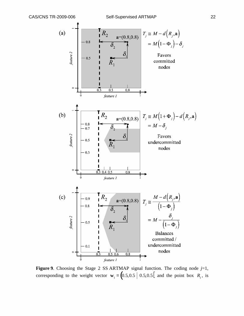
Figure 9. Choosing the Stage 2 SS ARTMAP signal function. The coding node j=1,
corresponding to the weight vector w
1= 0.5,0.5 0.5,0.5( ) and the point box R1
, is
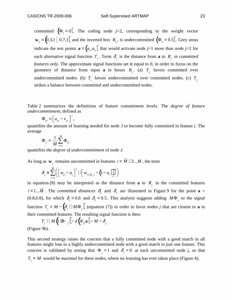
CAS/CNS TR-2009-006 Self-Supervised ARTMAP 23
committed Φ
1= 0( ). The coding node j=2, corresponding to the weight vector
w
2= 0.3,1 0.7,1( ) and the inverted box R2
, is undercommitted
Φ2
= 0.5( ). Grey areas
indicate the test points a = a
1,a
2( ) that would activate node j=1 more than node j=2 for
each alternative signal function T
j. Term
δ
j is the distance from a to
R
j in committed
features only. The approximate signal functions set α equal to 0, in order to focus on the geometry of distance from input a to boxes
R
j. (a)
T
j favors committed over
undercommitted nodes. (b) T
j favors undercommitted over committed nodes. (c)
T
j
strikes a balance between committed and undercommitted nodes. Table 2 summarizes the definitions of feature commitment levels. The degree of feature undercommitment, defined as
Φ
iJ= u
iJ− v
iJ
+,
quantifies the amount of learning needed for node J to become fully committed in feature i. The average
Φ
J= 1
MΦ
iJi =1
M
∑
quantifies the degree of undercommitment of node J. As long as
w
j remains uncommitted in features i = M + 1...M , the term
δ
j≡ w
ij− a
i
++ w
i + M , j− 1− a
i( )
+
i =1
M
∑
in equation (8) may be interpreted as the distance from a to R
j in the committed features
i = 1...M . The committed distances δ1 and δ2
are illustrated in Figure 9 for the point a =
(0.8,0.8), for which δ1= 0.6 and δ2
= 0.5. This analysis suggests adding MΦ
j to the signal
function T
j= M − δ
j+ MΦ
j( ) (equation (7)) in order to favor nodes j that are closest to a in
their committed features. The resulting signal function is then:
T
j≅
M 1+ Φ
j( )− d Rj,,a( )=
M − δ
j
(Figure 9b). This second strategy raises the concern that a fully committed node with a good match in all features might lose to a highly undercommitted node with a good match in just one feature. This concern is validated by noting that
Φ
j= 1 and
δ
j= 0 at each uncommitted node j, so that
T
j= M would be maximal for these nodes, where no learning has ever taken place (Figure 4).

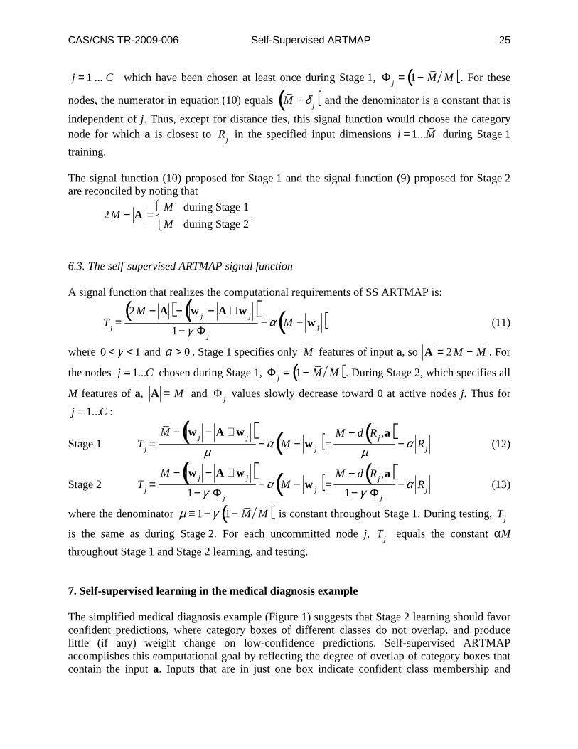
CAS/CNS TR-2009-006 Self-Supervised ARTMAP 24
Figure 9c suggests an alternative strategy for biasing T
j in such a way that undercommitted
nodes can compete for Stage 2 activation while respecting the specificity of learning at more committed nodes. Here,
T
j≅
M − d Rj,a( )
1− Φj( ) =
M − δj+ MΦ
j( )1− Φ
j( ) =
M −δ
j
1− Φj( ).
In Figure 9c, Φ1= 0 and
T
1= 2 − δ
1( ) at the committed node j=1, and Φ2= 0.5 and
T
2= 2 − 2δ
1( ) at the undercommitted node j=2. This third design strategy is implemented in
SS ARTMAP, though the full definition of T
j is perturbed to break distance ties and avoid
division by 0. 6.2. Balancing committed and uncommitted features during Stage 1 learning Analysis of Stage 2 learning (Figure 9) supports the signal function definition:
Tj =
M − w j − A ∧ w j( )1− γ Φ j
− α M − w j( ) =
M − d Rj ,a( )1− γ Φ j
− α Rj (9)
where 0 < γ < 1. When a node is committed
Φ j = 0( ), the signal function (9) reduces to the
ART choice-by-difference signal function (1). This definition is problematic, however, for Stage 1 learning. During Stage 1, where only M of the M input features are specified,
Ai =
ai if i=1...M
1− ai( ) if i= 1+ M( )... M + M( )1 otherwise
.
At uncommitted nodes j, all wij = 1, so
w j = 2M and the degree of undercommitment
Φ j = 1.
Thus if j is an uncommitted node, the denominator in equation (9) equals 1− γ( ), which is
typically small. Hence the only way to keep uncommitted nodes from overwhelming the coding pattern y is to require that the signal function numerator equal 0 when
Φ j = 1. For an
uncommitted node j during Stage 1,
d Rj ,a( )= w j − A ∧ w j = 2M − 2M − M( )= M .
This analysis suggests that the Stage 2 signal function of equation (9) needs to be modified for Stage 1 to:
Tj =
M − w j − A ∧ w j( )1− γ Φ j
− α M − w j( ) =
M − d Rj ,A( )1− γ Φ j
− α Rj (10)
For the Stage 1 signal function (10),
Tj = α M when j is an uncommitted node. For nodes
CAS/CNS TR-2009-006 Self-Supervised ARTMAP 25
j = 1 ... C which have been chosen at least once during Stage 1, Φ j = 1− M M( ). For these
nodes, the numerator in equation (10) equals
M − δ j( ) and the denominator is a constant that is
independent of j. Thus, except for distance ties, this signal function would choose the category node for which a is closest to
Rj in the specified input dimensions i = 1...M during Stage 1
training. The signal function (10) proposed for Stage 1 and the signal function (9) proposed for Stage 2 are reconciled by noting that
2M − A =
M during Stage 1
M during Stage 2
.
6.3. The self-supervised ARTMAP signal function A signal function that realizes the computational requirements of SS ARTMAP is:
Tj =
2M − A( )− w j − A ∧ w j( )1− γ Φ j
− α M − w j( ) (11)
where 0 < γ < 1 and α > 0 . Stage 1 specifies only M features of input a, so A = 2M − M . For
the nodes j = 1...C chosen during Stage 1, Φ j = 1− M M( ). During Stage 2, which specifies all
M features of a, A = M and
Φ j values slowly decrease toward 0 at active nodes j. Thus for
j = 1...C :
Stage 1 Tj =
M − w j − A ∧ w j( )µ
− α M − w j( )=
M − d Rj ,a( )µ
− α Rj (12)
Stage 2
Tj =
M − w j − A ∧ w j( )1− γ Φ j
− α M − w j( )=
M − d Rj ,a( )1− γ Φ j
− α Rj (13)
where the denominator µ ≡ 1− γ 1− M M( ) is constant throughout Stage 1. During testing,
Tj
is the same as during Stage 2. For each uncommitted node j, Tj equals the constant αM
throughout Stage 1 and Stage 2 learning, and testing. 7. Self-supervised learning in the medical diagnosis example The simplified medical diagnosis example (Figure 1) suggests that Stage 2 learning should favor confident predictions, where category boxes of different classes do not overlap, and produce little (if any) weight change on low-confidence predictions. Self-supervised ARTMAP accomplishes this computational goal by reflecting the degree of overlap of category boxes that contain the input a. Inputs that are in just one box indicate confident class membership and
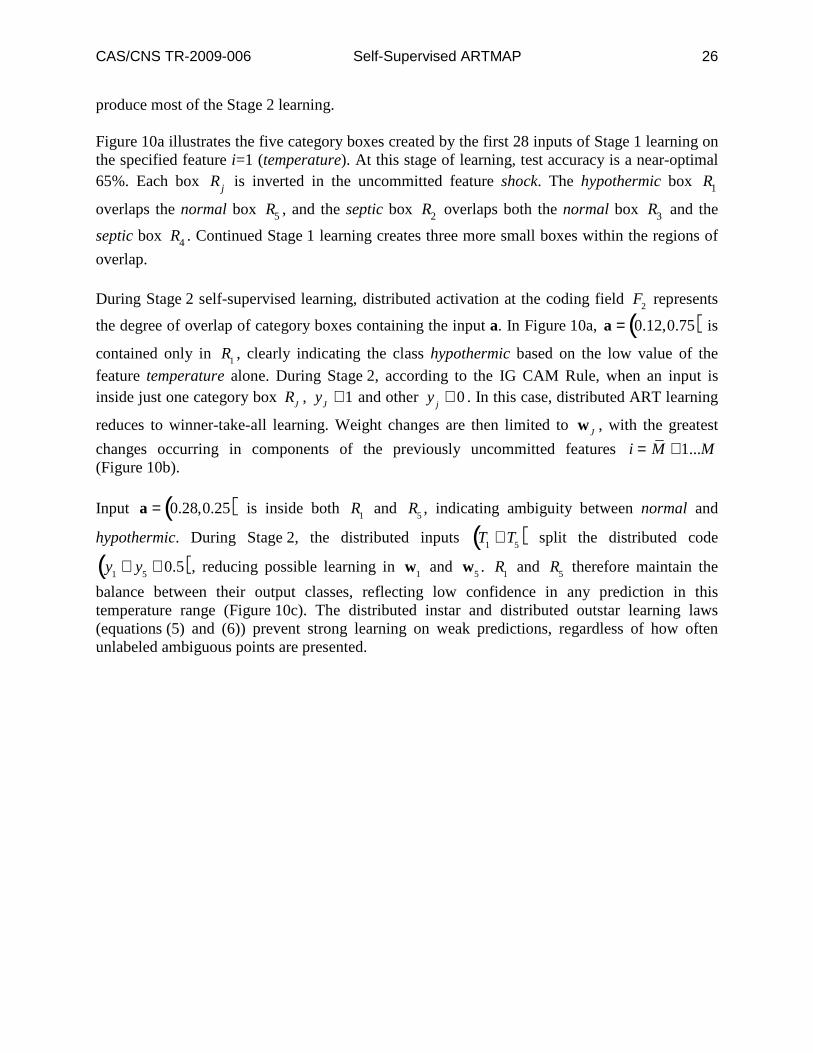
CAS/CNS TR-2009-006 Self-Supervised ARTMAP 26
produce most of the Stage 2 learning. Figure 10a illustrates the five category boxes created by the first 28 inputs of Stage 1 learning on the specified feature i=1 (temperature). At this stage of learning, test accuracy is a near-optimal 65%. Each box
Rj is inverted in the uncommitted feature shock. The hypothermic box
R1
overlaps the normal box R5 , and the septic box
R2 overlaps both the normal box
R3 and the
septic box R4 . Continued Stage 1 learning creates three more small boxes within the regions of
overlap. During Stage 2 self-supervised learning, distributed activation at the coding field F2
represents
the degree of overlap of category boxes containing the input a. In Figure 10a, a = 0.12,0.75( ) is
contained only in R1, clearly indicating the class hypothermic based on the low value of the
feature temperature alone. During Stage 2, according to the IG CAM Rule, when an input is inside just one category box RJ
, yJ≅ 1 and other
y
j≅ 0 . In this case, distributed ART learning
reduces to winner-take-all learning. Weight changes are then limited to wJ, with the greatest
changes occurring in components of the previously uncommitted features i = M + 1...M (Figure 10b).
Input a = 0.28,0.25( ) is inside both R1
and R5, indicating ambiguity between normal and
hypothermic. During Stage 2, the distributed inputs T
1≅ T
5( ) split the distributed code
y
1≅ y
5≅ 0.5( ), reducing possible learning in w1
and w5. R1
and R5 therefore maintain the
balance between their output classes, reflecting low confidence in any prediction in this temperature range (Figure 10c). The distributed instar and distributed outstar learning laws (equations (5) and (6)) prevent strong learning on weak predictions, regardless of how often unlabeled ambiguous points are presented.
CAS/CNS TR-2009-006 Self-Supervised ARTMAP 27
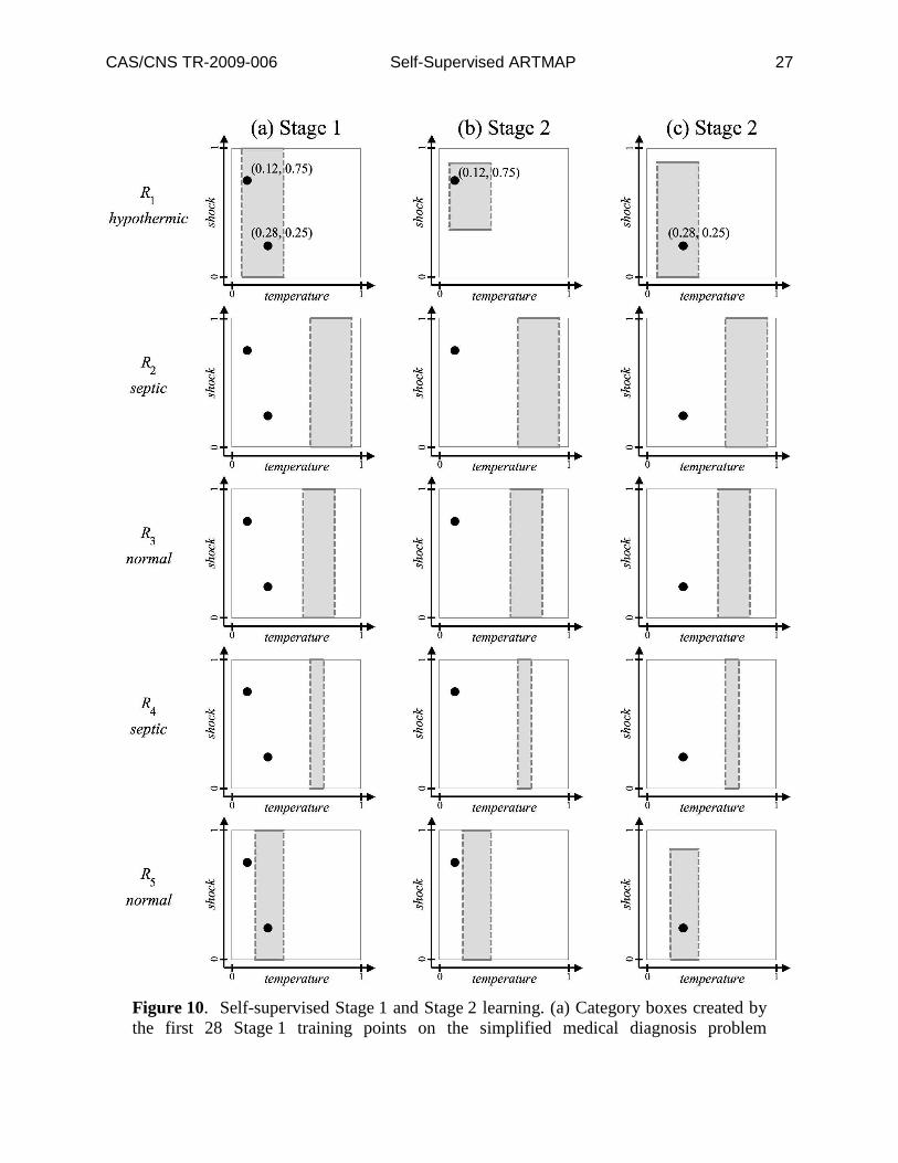
Figure 10. Self-supervised Stage 1 and Stage 2 learning. (a) Category boxes created by the first 28 Stage 1 training points on the simplified medical diagnosis problem
CAS/CNS TR-2009-006 Self-Supervised ARTMAP 28
(Figure 1). Boxes are inverted in the uncommitted feature i=1 (shock), as indicated by the dashed edges. (b) When the unlabeled point a = (0.12, 0.75) is presented during Stage 2, it activates only node j=1. During learning,
R1 (hypothermic) contracts toward the high
shock value of this input. (c) When the point a = (0.28, 0.25) is presented during Stage 2, it activates nodes j=1 and j=5, which share distributed activations, allowing relatively small weight updates in this case of ambiguous class predictions. All parameter values are as specified in Table 5, except that the Stage 2 learning rate is uncharacteristically
high
β = 0.5( ), which speeds up learning so as to make weight changes visible in this
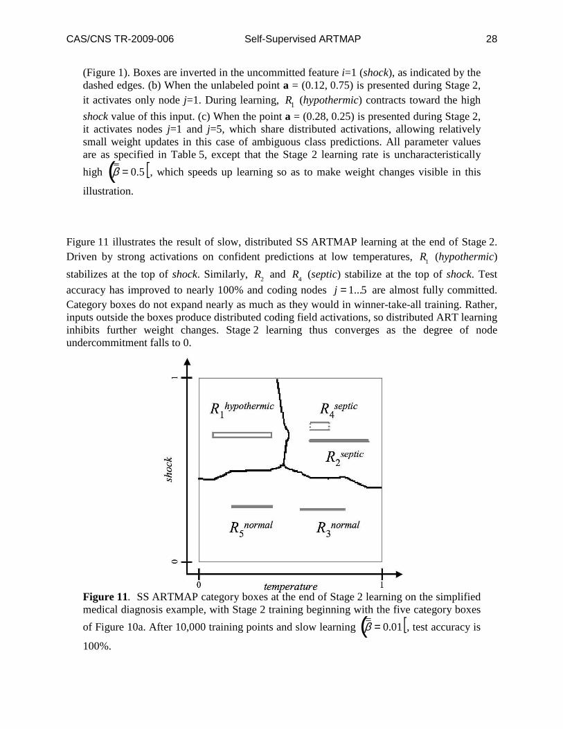
illustration. Figure 11 illustrates the result of slow, distributed SS ARTMAP learning at the end of Stage 2. Driven by strong activations on confident predictions at low temperatures, R1
(hypothermic)
stabilizes at the top of shock. Similarly, R2 and R4
(septic) stabilize at the top of shock. Test
accuracy has improved to nearly 100% and coding nodes j = 1...5 are almost fully committed. Category boxes do not expand nearly as much as they would in winner-take-all training. Rather, inputs outside the boxes produce distributed coding field activations, so distributed ART learning inhibits further weight changes. Stage 2 learning thus converges as the degree of node undercommitment falls to 0.
Figure 11. SS ARTMAP category boxes at the end of Stage 2 learning on the simplified medical diagnosis example, with Stage 2 training beginning with the five category boxes
of Figure 10a. After 10,000 training points and slow learning β = 0.01( ), test accuracy is
100%.
CAS/CNS TR-2009-006 Self-Supervised ARTMAP 29
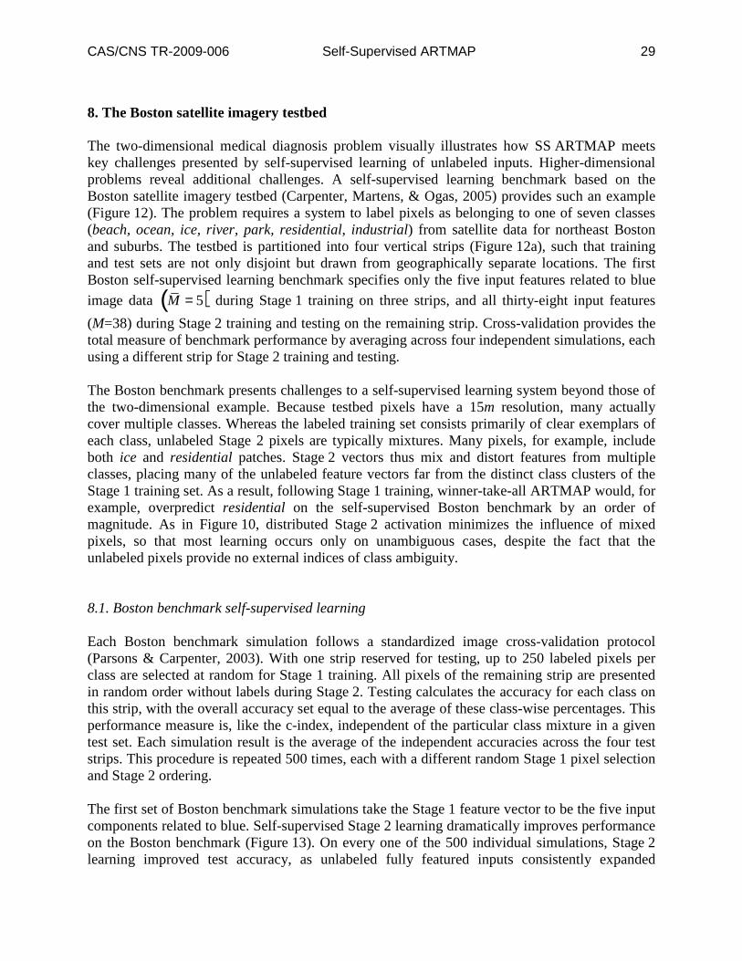
8. The Boston satellite imagery testbed The two-dimensional medical diagnosis problem visually illustrates how SS ARTMAP meets key challenges presented by self-supervised learning of unlabeled inputs. Higher-dimensional problems reveal additional challenges. A self-supervised learning benchmark based on the Boston satellite imagery testbed (Carpenter, Martens, & Ogas, 2005) provides such an example (Figure 12). The problem requires a system to label pixels as belonging to one of seven classes (beach, ocean, ice, river, park, residential, industrial) from satellite data for northeast Boston and suburbs. The testbed is partitioned into four vertical strips (Figure 12a), such that training and test sets are not only disjoint but drawn from geographically separate locations. The first Boston self-supervised learning benchmark specifies only the five input features related to blue
image data
M = 5( ) during Stage 1 training on three strips, and all thirty-eight input features
(M=38) during Stage 2 training and testing on the remaining strip. Cross-validation provides the total measure of benchmark performance by averaging across four independent simulations, each using a different strip for Stage 2 training and testing. The Boston benchmark presents challenges to a self-supervised learning system beyond those of the two-dimensional example. Because testbed pixels have a 15m resolution, many actually cover multiple classes. Whereas the labeled training set consists primarily of clear exemplars of each class, unlabeled Stage 2 pixels are typically mixtures. Many pixels, for example, include both ice and residential patches. Stage 2 vectors thus mix and distort features from multiple classes, placing many of the unlabeled feature vectors far from the distinct class clusters of the Stage 1 training set. As a result, following Stage 1 training, winner-take-all ARTMAP would, for example, overpredict residential on the self-supervised Boston benchmark by an order of magnitude. As in Figure 10, distributed Stage 2 activation minimizes the influence of mixed pixels, so that most learning occurs only on unambiguous cases, despite the fact that the unlabeled pixels provide no external indices of class ambiguity. 8.1. Boston benchmark self-supervised learning Each Boston benchmark simulation follows a standardized image cross-validation protocol (Parsons & Carpenter, 2003). With one strip reserved for testing, up to 250 labeled pixels per class are selected at random for Stage 1 training. All pixels of the remaining strip are presented in random order without labels during Stage 2. Testing calculates the accuracy for each class on this strip, with the overall accuracy set equal to the average of these class-wise percentages. This performance measure is, like the c-index, independent of the particular class mixture in a given test set. Each simulation result is the average of the independent accuracies across the four test strips. This procedure is repeated 500 times, each with a different random Stage 1 pixel selection and Stage 2 ordering. The first set of Boston benchmark simulations take the Stage 1 feature vector to be the five input components related to blue. Self-supervised Stage 2 learning dramatically improves performance on the Boston benchmark (Figure 13). On every one of the 500 individual simulations, Stage 2 learning improved test accuracy, as unlabeled fully featured inputs consistently expanded
CAS/CNS TR-2009-006 Self-Supervised ARTMAP 30
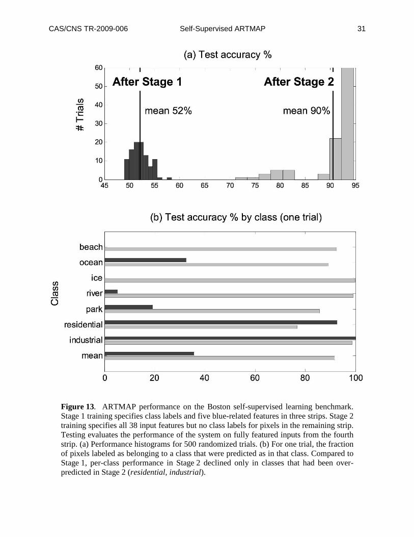
knowledge from Stage 1 training. Following Stage 1 (dark bars, Figure 13a), the class-based test accuracy was between 50% and 58% across the 500 simulations. Stage 2 self-supervised learning, with all 38 features specified, improved accuracy on each simulation to above 70%, with a mean of 90% (light bars). Figure 13b displays test accuracy on each class for a typical SS ARTMAP trial. Note, for example, that Stage 2 learning improves accuracy of ice ground-truth pixels from 0% (Stage 1) to 99%.
Figure 12. The satellite image and labeled ground-truth pixels for the Boston testbed (http://techlab.bu.edu/classer/data_sets). Only 28,735 of the 216,000 pixels are labeled, of which only 6,634 represent classes other than ocean. (a) Cross-validation divides the testbed into four vertical strips. (b) Class distributions vary substantially across strips. For example, the right-hand strip contains mainly ocean pixels (dark), while the left-hand strip contains neither ocean nor beach pixels.
CAS/CNS TR-2009-006 Self-Supervised ARTMAP 31
Figure 13. ARTMAP performance on the Boston self-supervised learning benchmark. Stage 1 training specifies class labels and five blue-related features in three strips. Stage 2 training specifies all 38 input features but no class labels for pixels in the remaining strip. Testing evaluates the performance of the system on fully featured inputs from the fourth strip. (a) Performance histograms for 500 randomized trials. (b) For one trial, the fraction of pixels labeled as belonging to a class that were predicted as in that class. Compared to Stage 1, per-class performance in Stage 2 declined only in classes that had been over-predicted in Stage 2 (residential, industrial).
CAS/CNS TR-2009-006 Self-Supervised ARTMAP 32
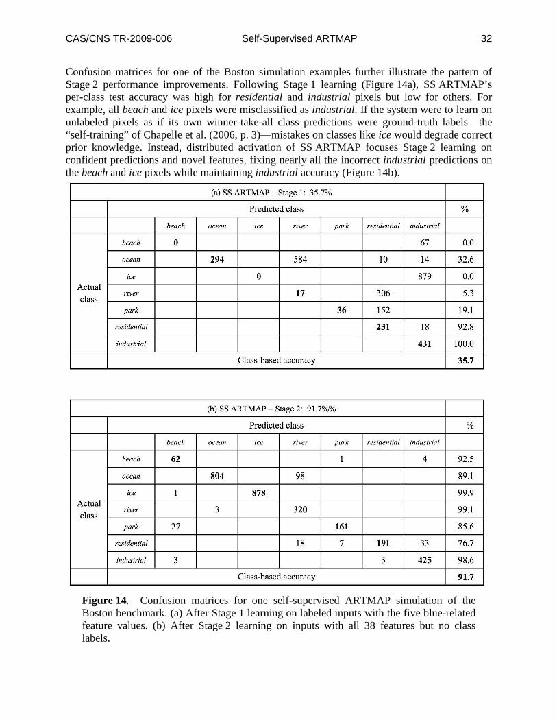
Confusion matrices for one of the Boston simulation examples further illustrate the pattern of Stage 2 performance improvements. Following Stage 1 learning (Figure 14a), SS ARTMAP’s per-class test accuracy was high for residential and industrial pixels but low for others. For example, all beach and ice pixels were misclassified as industrial. If the system were to learn on unlabeled pixels as if its own winner-take-all class predictions were ground-truth labels—the “self-training” of Chapelle et al. (2006, p. 3)—mistakes on classes like ice would degrade correct prior knowledge. Instead, distributed activation of SS ARTMAP focuses Stage 2 learning on confident predictions and novel features, fixing nearly all the incorrect industrial predictions on the beach and ice pixels while maintaining industrial accuracy (Figure 14b).
Figure 14. Confusion matrices for one self-supervised ARTMAP simulation of the Boston benchmark. (a) After Stage 1 learning on labeled inputs with the five blue-related feature values. (b) After Stage 2 learning on inputs with all 38 features but no class labels.
CAS/CNS TR-2009-006 Self-Supervised ARTMAP 33
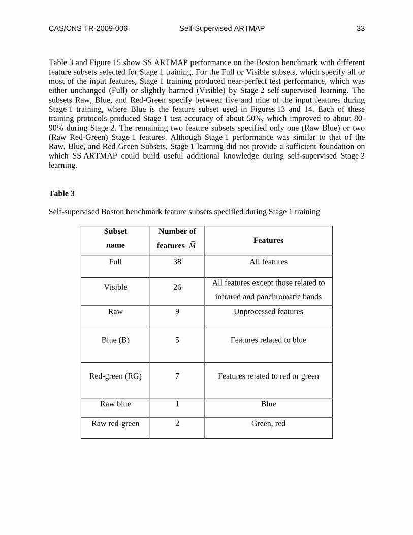
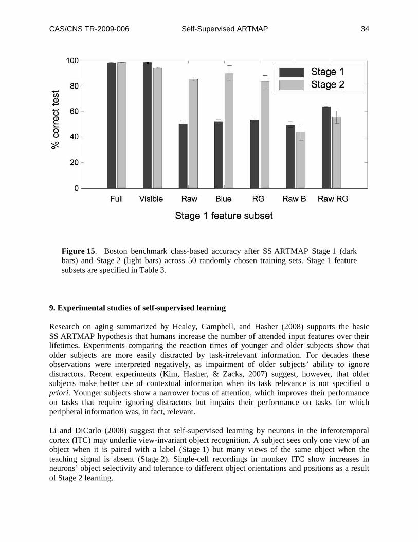
Table 3 and Figure 15 show SS ARTMAP performance on the Boston benchmark with different feature subsets selected for Stage 1 training. For the Full or Visible subsets, which specify all or most of the input features, Stage 1 training produced near-perfect test performance, which was either unchanged (Full) or slightly harmed (Visible) by Stage 2 self-supervised learning. The subsets Raw, Blue, and Red-Green specify between five and nine of the input features during Stage 1 training, where Blue is the feature subset used in Figures 13 and 14. Each of these training protocols produced Stage 1 test accuracy of about 50%, which improved to about 80-90% during Stage 2. The remaining two feature subsets specified only one (Raw Blue) or two (Raw Red-Green) Stage 1 features. Although Stage 1 performance was similar to that of the Raw, Blue, and Red-Green Subsets, Stage 1 learning did not provide a sufficient foundation on which SS ARTMAP could build useful additional knowledge during self-supervised Stage 2 learning.
Table 3
Self-supervised Boston benchmark feature subsets specified during Stage 1 training
Subset
name
Number of
features M
Features
Full 38 All features
Visible 26 All features except those related to
infrared and panchromatic bands
Raw 9 Unprocessed features
Blue (B) 5 Features related to blue
Red-green (RG) 7 Features related to red or green
Raw blue 1 Blue
Raw red-green 2 Green, red
CAS/CNS TR-2009-006 Self-Supervised ARTMAP 34
Figure 15. Boston benchmark class-based accuracy after SS ARTMAP Stage 1 (dark bars) and Stage 2 (light bars) across 50 randomly chosen training sets. Stage 1 feature subsets are specified in Table 3.
9. Experimental studies of self-supervised learning Research on aging summarized by Healey, Campbell, and Hasher (2008) supports the basic SS ARTMAP hypothesis that humans increase the number of attended input features over their lifetimes. Experiments comparing the reaction times of younger and older subjects show that older subjects are more easily distracted by task-irrelevant information. For decades these observations were interpreted negatively, as impairment of older subjects’ ability to ignore distractors. Recent experiments (Kim, Hasher, & Zacks, 2007) suggest, however, that older subjects make better use of contextual information when its task relevance is not specified a priori . Younger subjects show a narrower focus of attention, which improves their performance on tasks that require ignoring distractors but impairs their performance on tasks for which peripheral information was, in fact, relevant. Li and DiCarlo (2008) suggest that self-supervised learning by neurons in the inferotemporal cortex (ITC) may underlie view-invariant object recognition. A subject sees only one view of an object when it is paired with a label (Stage 1) but many views of the same object when the teaching signal is absent (Stage 2). Single-cell recordings in monkey ITC show increases in neurons’ object selectivity and tolerance to different object orientations and positions as a result of Stage 2 learning.
CAS/CNS TR-2009-006 Self-Supervised ARTMAP 35
Smith and Minda (2000) summarized thirty experiments on human pattern learning and classification. In each experiment, subjects unlearn in a characteristic way exemplars they had learned to classify perfectly during training. In Amis, Carpenter, Ersoy, and Grossberg (2009), ARTMAP simulations fit the experimental data and explain how classification patterns are learned and forgotten in real time. The model tests two competing hypotheses: (a) that the observed forgetting is the result of an unsupervised learning process; and (b) that the forgetting is the result of a corruption of long-term memory (LTM) traces by noise. The noise hypothesis (b) better fits the data and is also consistent with the mechanisms of self-supervised ARTMAP. Distributed learning during Stage 2 focuses LTM adaptation on input features whose values were unspecified during Stage 1. The unsupervised hypothesis (a) is equivalent to Stage 2 learning but with no novel input features specified, and so not enough additional learning occurs to model the data. 10. Related models of self-supervised learning SS ARTMAP introduces a new definition of self-supervised learning: a system trained on labeled data with limited features continues to learn on an expanded but unlabeled feature set. As such, no prior work directly addresses this learning paradigm. There are, however, many studies related to this form of self-supervised learning. Semi-supervised learning incorporates labeled and unlabeled inputs in its supervised training set, but unlike self-supervised learning, all inputs have the same number of specified feature values. Without any novel features from which to learn, semi-supervised learning systems use the unlabeled data to refine the model parameters defined using the labeled data. Reviews of semi-supervised learning (Chapelle, Schölkopf, & Zien, 2006; Zhu, 2005) find that its success is sensitive to underlying data distributions, in particular to whether data cluster or lie on a lower-dimensional manifold. Typically, models must be carefully selected and tuned for each problem space, using a priori knowledge of the domain. Chapelle et al. (2006) conclude that none of the semi-supervised models they reviewed is robust enough to be considered general purpose, and that semi-supervised learning remains an open problem. The main difficulty is that, whenever the unlabeled data are different enough from the labeled data to merit learning, it is unclear whether differences are useful, or whether they are the result of noise or other distortions that would damage the system’s performance. Another class of models admits inputs with different numbers of features, but in a different context than self-supervised ARTMAP learning. These methods assume that feature values are missing randomly and infrequently, and thus can be filled in based on a statistical analysis of other exemplars in the training set (Little & Rubin, 2002). Some applications add missing feature estimates to neural network architectures such as fuzzy ARTMAP (Lim, Leong, & Kuan, 2005) or multilayer perceptrons (Tresp, Neuneier, & Ahmad, 1995). Whereas feature estimates can succeed for problems with stationary statistics and redundant training data, challenging problems risk inappropriate learning on filled-in values. For this reason, exemplars with missing feature values are often excluded from the training set. In many situations, however, data points for an
CAS/CNS TR-2009-006 Self-Supervised ARTMAP 36
entire cluster, class, or dataset have a common set of unspecified feature values. Structurally missing features are either ignored or substituted, and typical solutions are specific to a particular model architecture. For example, Chechik, Heitz, Elidan, Abbeel, and Koller (2008) created a support vector machine (SVM) that redefines the margin maximization objective to ignore unspecified feature values. Ishibuchi, Miyazaki, Kwon, and Tanaka (1993) modified a multilayer perceptron such that hidden layer nodes track feature value intervals rather than scalar values, representing a missing feature value as the interval [0,1]. 11. Conclusion Self-supervised ARTMAP defines a novel problem space that may be tested on almost any existing dataset designed for supervised learning. The system learns during an initial “textbook” supervised learning phase that is followed by a “real world” unsupervised learning phase. The novel aspect of the SS ARTMAP learning protocol is that inputs of the second, self-supervised phase specify more features than did the labeled inputs of the first phase. The expanded feature set provides to a learning system the capacity to teach the network important new information, so that accuracy may improve dramatically compared to that of the initial trained system, while avoiding performance deterioration from unlabeled data. New problem domains include applications in which a trained system performs in novel contexts, such as an image recognition problem in which an initial set of sensor data is later augmented on-line with unlabeled data from a new sensor. Acknowledgements This research was supported by the SyNAPSE program of the Defense Advanced Projects
Research Agency (Hewlett-Packard Company, subcontract under DARPA prime contract HR0011-09-3-0001; and HRL Laboratories LLC, subcontract #801881-BS under DARPA prime contract HR0011-09-C-0001) and by CELEST, an NSF Science of Learning Center (SBE-0354378).
CAS/CNS TR-2009-006 Self-Supervised ARTMAP 37
References Amis, G.P., & Carpenter, G.A. (2007). Default ARTMAP 2. Proceedings of the International
Joint Conference on Neural Networks (IJCNN’07 – Orlando, Florida), 777-782. http://techlab.bu.edu/members/gail/articles/152_Default_ARTMAP2_2007_.pdf Amis, G.P., Carpenter, G.A., Ersoy, B., & Grossberg, S. (2009). Cortical learning of recognition
categories: a resolution of the exemplar vs. prototype debate. Technical Report, CAS/CNS TR-2009-002, Boston, MA: Boston University.
Carpenter, G.A. (1994). A distributed outstar network for spatial pattern learning. Neural
Networks, 7, 159-168. http://techlab.bu.edu/members/gail/articles/083_dOutstar_1994_.pdf Carpenter G. A. (1997). Distributed learning, recognition, and prediction by ART and ARTMAP
neural networks. Neural Networks, 10, 1473–1494. http://techlab.bu.edu/members/gail/articles/115_dART_NN_1997_.pdf Carpenter, G. A. (2003). Default ARTMAP. Proceedings of the international joint conference on
neural networks (IJCNN’03), 1396–1401. http://techlab.bu.edu/members.gail/articles/142_Default_ARTMAP_2003_.pdf Carpenter, G.A., & Gjaja, M.N. (1994). Fuzzy ART choice functions. Proceedings of the World
Congress on Neural Networks (WCNN-94), Hillsdale, NJ: Lawrence Erlbaum Associates, I-713-722. http://techlab.bu.edu/files/resources/articles_cns/CarpenterGjaja1994.pdf
Carpenter G. A., & Grossberg S. (1987). A massively parallel architecture for a self-organizing
neural pattern recognition machine. Computer Vision, Graphics, and Image Processing, 37, 54–115. http://techlab.bu.edu/members/gail/articles/026_ART_1_CVGIP_1987.pdf
Carpenter, G. A., & Grossberg, S. (1990). ART 3: Hierarchical search using chemical
transmitters in self-organizing pattern recognition architectures. Neural Networks, 4, 129-152. http://techlab.bu.edu/members/gail/articles/042_ART_3_1990_.pdf
Carpenter G. A., Grossberg S., Markuzon N., Reynolds J. H., & Rosen D. B. (1992). Fuzzy
ARTMAP: A neural network architecture for incremental supervised learning of analog multidimensional maps. IEEE Transactions on Neural Networks, 3, 698–713.
http://techlab.bu.edu/members/gail/articles/070_Fuzzy_ARTMAP_1992_.pdf Carpenter G. A., Grossberg S., & Reynolds J. H. (1991a). ARTMAP: Supervised real-time
learning and classification of nonstationary data by a self-organizing neural network. Neural Networks, 4, 565–588.
http://techlab.bu.edu/members/gail/articles/054_ARTMAP_1991_.pdf
CAS/CNS TR-2009-006 Self-Supervised ARTMAP 38
Carpenter, G. A., Grossberg S., & Rosen D. B. (1991b). Fuzzy ART: Fast stable learning and
categorization of analog patterns by an adaptive resonance system. Neural Networks, 4, 759–771. http://techlab.bu.edu/members/gail/articles/056_Fuzzy_ART_1991_.pdf
Carpenter, G.A., & N. Markuzon, N. (1998). ARTMAP-IC and medical diagnosis: Instance
counting and inconsistent cases. Neural Networks, 11, 323-336. http://techlab.bu.edu/members/gail/articles/117_ARTMAP-IC_1998_.pdf Carpenter, G.A., Martens, S., & Ogas, O.J. (2005). Self-organizing information fusion and
hierarchical knowledge discovery: a new framework using ARTMAP neural networks. Neural Networks, 18, 287-295.
http://techlab.bu.edu/members/gail/articles/148_2005_InfoFusion_CarpenterMartensOgas_.pdf Carpenter, G.A., Milenova, B.L., & Noeske, B.W. (1998). Distributed ARTMAP: a neural
network for fast distributed supervised learning. Neural Networks, 11, 793-813. http://techlab.bu.edu/members/gail/articles/120_dARTMAP_1998_.pdf Carpenter. G.A., & Ross, W.D. (1995). ART-EMAP: A neural network architecture for object
recognition by evidence accumulation. IEEE Transactions on Neural Networks, 6, 805-818, 1995. http://techlab.bu.edu/members/gail/articles/097_ART-EMAP_1995_.pdf
Chapelle, O., Schölkopf, B., & Zien, A. (Eds.). (2006). Semi-supervised learning. Cambridge,
MA: MIT Press. Chechik, G., Heitz, G., Elidan, G., Abbeel, P., & Koller, D. (2008). Max Margin classification of
incomplete data. Journal of Machine Learning Research, 9, 1-21. http://portal.acm.org/citation.cfm?id=1390681.1390682 Grossberg, S. (1968). Some nonlinear networks capable of learning a spatial pattern of arbitrary
complexity. Proceedings of the National Academy of Sciences, 59, 368-372. http://cns.bu.edu/~steve/Gro1968PNAS59.pdf Grossberg, S. (1976). Adaptive pattern classification and universal recoding. I: Parallel
development and coding of neural feature detectors. Biological Cybernetics, 23, 121-134. http://cns.bu.edu/~steve/Gro1976BiolCyb_I.pdf Healey, M.K., Campbell, K.L., & Hasher, L. (2008). Cognitive aging and increased
distractibility: costs and potential benefits. In W.S. Sossin, J.-C. Lacaille, V.F. Castellucci, & S. Belleville (Eds.), Progress in Brain Research, 129, 353-363.
http://www.ncbi.nlm.nih.gov/pubmed/18394486 Ishibuchi, H., Miyazaki, A., Kwon, K., & Tanaka, H. (1993). Learning from incomplete training
data with missing values and medical application. Proceedings of the IEEE International Joint Conference on Neural Networks (IJCNN’93), 1871-1874.
http://ieeexplore.ieee.org/xpl/freeabs_all.jsp?arnumber=717020
CAS/CNS TR-2009-006 Self-Supervised ARTMAP 39
Kim, S., Hasher, K., & Zacks, R.T. (2007). Aging and a benefit of distractibility. Psychonomic
Bulletin and Review. 14, 301-305. http://www.pubmedcentral.nih.gov/articlerender.fcgi?artid=2121579 Krashen, S. (2004, November). Applying the comprehension hypothesis: Some suggestions.
Presented at 13th International Symposium and Book Fair on Language Teaching (English Teachers Association of the Republic of China), Taipei, Taiwan.
http://www.sdkrashen.com/articles/eta_paper/ Li, N., & DiCarlo, J.J. (2008). Unsupervised natural experience rapidly alters invariant object
representation in visual cortex. Science, 321(5895), 1502-1507. http://www.sciencemag.org/cgi/content/abstract/321/5895/1502 Lim, C., Leong, J., & Kuan, M. (2005). A hybrid neural network system for pattern classification
tasks with missing features. IEEE Transactions on Pattern Analysis and Machine Intelligence, 27(4), 648-653.
http://www2.computer.org/portal/web/csdl/doi/10.1109/TPAMI.2005.64 Little, R., & Rubin, D. (2002). Statistical analysis with missing data (2nd Ed.). New York: Wiley
Interscience. Parsons, O., & Carpenter, G. A. (2003). ARTMAP neural networks for information fusion and
data mining: map production and target recognition methodologies. Neural Networks, 16, 1075-1089. http://techlab.bu.edu/members/gail/articles/143_ARTMAP_map_NN_2003_.pdf
Smith, J.D., & Minda, J.P. (2000). Thirty categorization results in search of a model. Journal of
Experimental Psychology: Learning, Memory, and Cognition, 26, 3-27. Tresp, V., Neuneier, R., & Ahmad, S. (1995). Efficient methods for dealing with missing data in
supervised learning. Proceedings of Advances in Neural Information Processing Systems (NIPS), 7, 689-696.
http://citeseerx.ist.psu.edu/viewdoc/download?doi=10.1.1.62.6142&rep=rep1&type=pdf Williamson, J.R. (1996). Gaussian ARTMAP: A neural network for fast incremental learning of
noisy multidimensional maps. Neural Networks, 9(5), 881-897. http://techlab.bu.edu/files/resources/articles_tt/Gaussian%20ARTMAP,%20A%20neural
%20network%20for%20past%20incremental%20learning%20of%20noisy%20multidimensional%20maps.pdf
Zhu, X. (2005). Semi-supervised learning literature survey. Technical Report 1530, Computer
Sciences, University of Wisconsin-Madison. Updated July 19, 2008. http://pages.cs.wisc.edu/~jerryzhu/pub/ssl_survey.pdf
CAS/CNS TR-2009-006 Self-Supervised ARTMAP 40
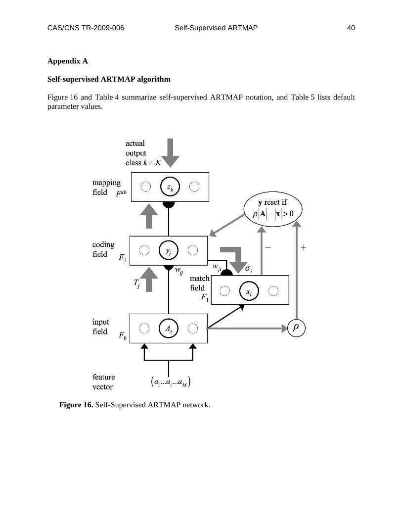
Appendix A Self-supervised ARTMAP algorithm Figure 16 and Table 4 summarize self-supervised ARTMAP notation, and Table 5 lists default parameter values.
Figure 16. Self-Supervised ARTMAP network.

CAS/CNS TR-2009-006 Self-Supervised ARTMAP 41
Table 4
Self-Supervised ARTMAP Notation
Notation Description
i input component index
j coding node index
k output class index
M number of input features specified during Stage 2 learning and testing
M number of features specified during Stage1 learning, M ≤ M
a feature vector a
i( ), 0 ≤ ai
≤ 1, i = 1,…,M
A complement coded input vector (Ai), i = 1,…,2M
K actual output class for an input
K' predicted output class
J chosen coding node (winner-take-all)
C number of activated coding nodes
ΛΛΛΛ , ′ΛΛΛΛ coding node index subsets
Tj signal from input field to coding node j
y coding field activation pattern (yj)
σ i signal from coding field to match field node i
kσ signal from coding field to output node k
w
ij
F0→ F
2 bottom-up weights from input node i to coding node j
w
ji
F2→ F
1 top-down weights from coding node j to match field node i

CAS/CNS TR-2009-006 Self-Supervised ARTMAP 42
jΦ degree of undercommitment of coding node j
jκ output class associated with coding node j
ρ vigilance variable
∧ component-wise minimum (fuzzy intersection): ( ) { }min ,i iip q∧ =p q
∨ component-wise maximum (fuzzy union): p ∨ q( )
i= max p
i, q
i{ }
⋅ vector size ( L1-norm): ii
p≡∑p
[ ]+⋅ rectification: [ ] { }max , 0p p+ =
CAS/CNS TR-2009-006 Self-Supervised ARTMAP 43
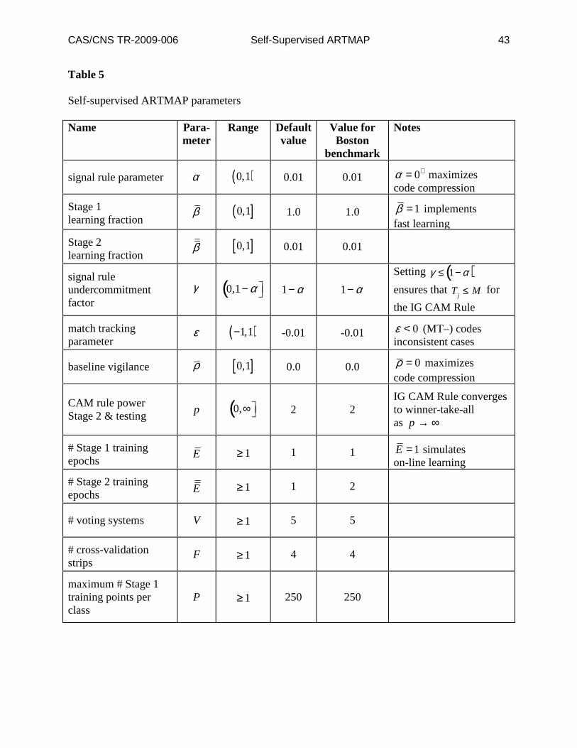
Table 5
Self-supervised ARTMAP parameters
Name Para- meter
Range Default value
Value for Boston
benchmark
Notes
signal rule parameter α ( )0,1 0.01 0.01 0α += maximizes code compression
Stage 1 learning fraction
β ( ]0,1 1.0 1.0 1β = implements fast learning
Stage 2 learning fraction
β [ ]0,1 0.01 0.01
signal rule undercommitment factor
γ 0,1− α( 1− α 1− α
Setting γ ≤ 1− α( )
ensures that T
j≤ M for
the IG CAM Rule
match tracking parameter
ε ( )1,1− -0.01 -0.01 0ε < (MT–) codes inconsistent cases
baseline vigilance ρ [ ]0,1 0.0 0.0 0ρ = maximizes code compression
CAM rule power Stage 2 & testing
p 0,∞( 2 2
IG CAM Rule converges to winner-take-all as p → ∞
# Stage 1 training epochs
E 1≥ 1 1 1E = simulates on-line learning
# Stage 2 training epochs E 1≥ 1 2
# voting systems V 1≥ 5 5
# cross-validation strips
F 1≥ 4 4
maximum # Stage 1 training points per class
P 1≥ 250 250
CAS/CNS TR-2009-006 Self-Supervised ARTMAP 44
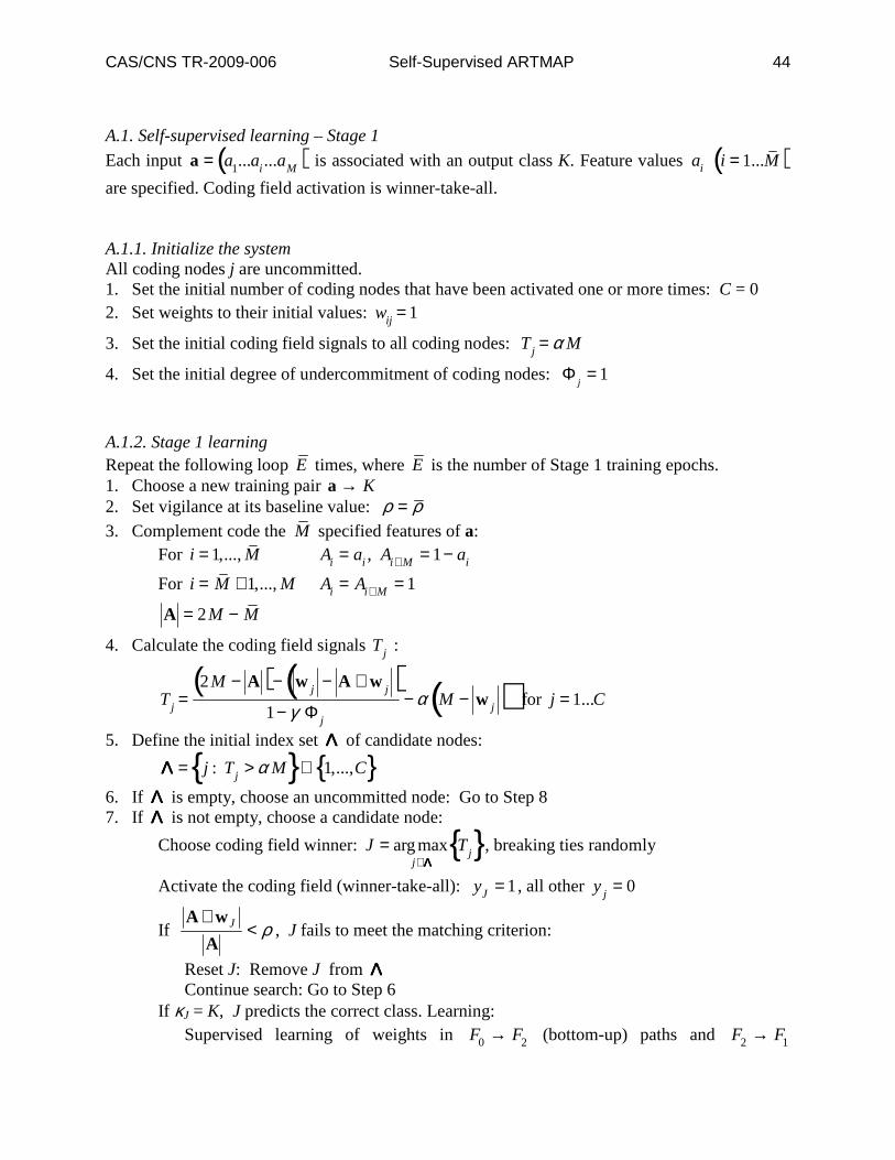
A.1. Self-supervised learning – Stage 1
Each input a = a1...ai ...aM( ) is associated with an output class K. Feature values
ai
i = 1...M( )
are specified. Coding field activation is winner-take-all. A.1.1. Initialize the system All coding nodes j are uncommitted. 1. Set the initial number of coding nodes that have been activated one or more times: C = 0 2. Set weights to their initial values:
wij = 1
3. Set the initial coding field signals to all coding nodes: Tj = α M
4. Set the initial degree of undercommitment of coding nodes: Φ
j= 1
A.1.2. Stage 1 learning Repeat the following loop E times, where E is the number of Stage 1 training epochs. 1. Choose a new training pair a → K 2. Set vigilance at its baseline value: ρ ρ= 3. Complement code the M specified features of a: For i = 1,...,M
Ai = ai , Ai + M = 1− ai
For i = M + 1,...,M Ai = Ai + M = 1
A = 2M − M
4. Calculate the coding field signals Tj :
Tj =
2M − A( )− w j − A ∧ w j( )1− γ Φ j
− α M − w j( ) for j = 1...C
5. Define the initial index set ΛΛΛΛ of candidate nodes:
ΛΛΛΛ = j : Tj > α M{ }⊆ 1,...,C{ }
6. If ΛΛΛΛ is empty, choose an uncommitted node: Go to Step 8 7. If ΛΛΛΛ is not empty, choose a candidate node:
Choose coding field winner: J = argmax
j ∈ΛΛΛΛTj{ }, breaking ties randomly
Activate the coding field (winner-take-all): yJ = 1, all other
y j = 0
If J ρ∧
<A w
A, J fails to meet the matching criterion:
Reset J: Remove J from ΛΛΛΛ Continue search: Go to Step 6 If κJ = K, J predicts the correct class. Learning: Supervised learning of weights in
F0 → F2 (bottom-up) paths and
F2 → F1
CAS/CNS TR-2009-006 Self-Supervised ARTMAP 45
(top-down) paths: wiJ = wJi = wiJ
old − β wiJold − Ai
+ for i = 1,…,2M.
With fast learning β = 1( ),
wiJ = wJi = Ai ∧ wiJ
old .
Update the degree of undercommitment of node J:
Φ
J= 1
Mw
iJ− 1− w
i + M ,J( )
+
i =1
M
∑
Continue to the next training pair: Go to Step 1 If κJ ≠ K, J predicts an incorrect class. Match tracking and reset:
Match track: Jρ ε∧
= +A w
A
Reset J: Remove J from ΛΛΛΛ Continue search: Go to Step 6 8. Activate a new node: Add 1 to the activated node count C ( )1,..., 2 ,iC i Cw A i M Kκ= = =
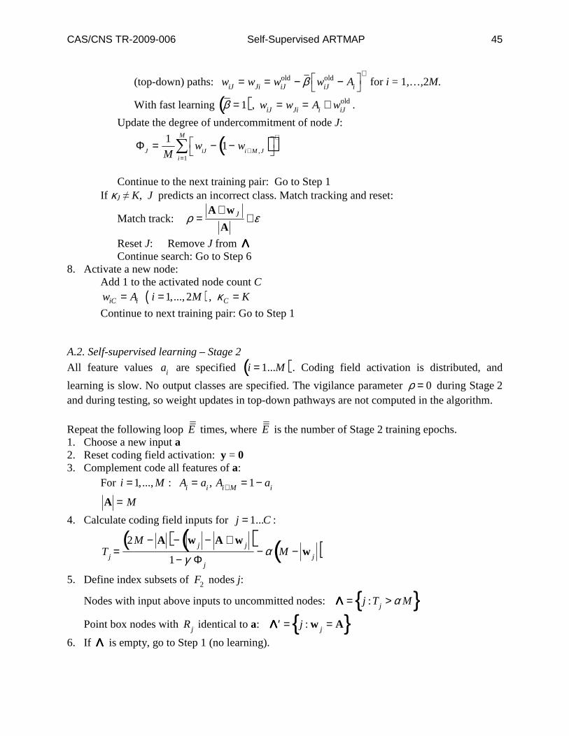
Continue to next training pair: Go to Step 1 A.2. Self-supervised learning – Stage 2
All feature values ai are specified
i = 1...M( ). Coding field activation is distributed, and
learning is slow. No output classes are specified. The vigilance parameter ρ = 0 during Stage 2 and during testing, so weight updates in top-down pathways are not computed in the algorithm.
Repeat the following loop E times, where E is the number of Stage 2 training epochs. 1. Choose a new input a 2. Reset coding field activation: y = 0 3. Complement code all features of a: For 1,...,i M= :
Ai = ai , Ai+ M = 1− ai
A = M
4. Calculate coding field inputs for j = 1...C :
Tj =
2M − A( )− w j − A ∧ w j( )1− γ Φ j
− α M − w j( ) 5. Define index subsets of
F2 nodes j:
Nodes with input above inputs to uncommitted nodes: ΛΛΛΛ = j :Tj > α M{ }
Point box nodes with Rj identical to a:
′ΛΛΛΛ = j : w j = A{ }
6. If ΛΛΛΛ is empty, go to Step 1 (no learning).
CAS/CNS TR-2009-006 Self-Supervised ARTMAP 46
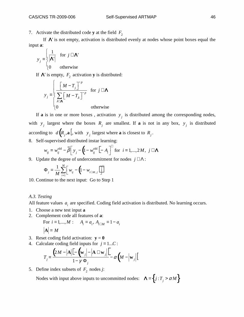
7. Activate the distributed code y at the field F2
If ′ΛΛΛΛ is not empty, activation is distributed evenly at nodes whose point boxes equal the input a:
y j =1
′ΛΛΛΛ for j ∈ ′ΛΛΛΛ
0 otherwise
If ′ΛΛΛΛ is empty, F2 activation y is distributed:
y j =
M − Tj
− p
M − Tλ − p
λ∈ΛΛΛΛ∑
for j ∈ΛΛΛΛ
0 otherwise
If a is in one or more boxes , activation y j is distributed among the corresponding nodes,
with y j largest where the boxes
Rj are smallest. If a is not in any box,
y j is distributed
according to d Rj ,a( ), with
y j largest where a is closest to
Rj .
8. Self-supervised distributed instar learning:
wij = wij
old − β y j − 1− wijold( )− Ai
+for i = 1,...,2M , j ∈ΛΛΛΛ
9. Update the degree of undercommitment for nodes j ∈Λ :
Φ
j= 1
Mw
ij− 1− w
i + M , j( )
+
i =1
M
∑
10. Continue to the next input: Go to Step 1 A.3. Testing All feature values
ai are specified. Coding field activation is distributed. No learning occurs.
1. Choose a new test input a 2. Complement code all features of a: For 1,...,i M= :
Ai = ai , Ai+ M = 1− ai
A = M
3. Reset coding field activation: y = 0 4. Calculate coding field inputs for j = 1...C :
Tj =
2M − A( )− w j − A ∧ w j( )1− γ Φ j
− α M − w j( ) 5. Define index subsets of
F2 nodes j:
Nodes with input above inputs to uncommitted nodes: ΛΛΛΛ = j :Tj > α M{ }
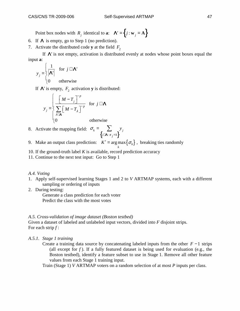
CAS/CNS TR-2009-006 Self-Supervised ARTMAP 47
Point box nodes with Rj identical to a:
′ΛΛΛΛ = j : w j = A{ }
6. If ΛΛΛΛ is empty, go to Step 1 (no prediction). 7. Activate the distributed code y at the field
F2
If ′ΛΛΛΛ is not empty, activation is distributed evenly at nodes whose point boxes equal the input a:
y j =1
′ΛΛΛΛ for j ∈ ′ΛΛΛΛ
0 otherwise
If ′ΛΛΛΛ is empty, F2 activation y is distributed:
y j =
M − Tj
− p
M − Tλ − p
λ∈ΛΛΛΛ∑
for j ∈ΛΛΛΛ
0 otherwise
8. Activate the mapping field:
σ k = y j
j∈ΛΛΛΛ: κ j =k{ }∑
9. Make an output class prediction: { }arg max kk
K σ′ = , breaking ties randomly
10. If the ground-truth label K is available, record prediction accuracy 11. Continue to the next test input: Go to Step 1 A.4. Voting 1. Apply self-supervised learning Stages 1 and 2 to V ARTMAP systems, each with a different
sampling or ordering of inputs 2. During testing: Generate a class prediction for each voter Predict the class with the most votes A.5. Cross-validation of image dataset (Boston testbed) Given a dataset of labeled and unlabeled input vectors, divided into F disjoint strips. For each strip f : A.5.1. Stage 1 training Create a training data source by concatenating labeled inputs from the other 1F − strips
(all except for f ). If a fully featured dataset is being used for evaluation (e.g., the Boston testbed), identify a feature subset to use in Stage 1. Remove all other feature values from each Stage 1 training input.
Train (Stage 1) V ARTMAP voters on a random selection of at most P inputs per class.

CAS/CNS TR-2009-006 Self-Supervised ARTMAP 48
A.5.2. Stage 2 training Train (Stage 2) each voter on a random ordering of all (fully featured) inputs in strip f,
including labeled and unlabeled inputs. A.5.3. Testing Generate ensemble class predictions on the fully featured, labeled inputs in f. Record per-class and average class accuracy.