Semantic Object Parsing with Graph LSTMusers.eecs.northwestern.edu/~xsh835/assets/eccv2016... · 2016-08-22 · Semantic Object Parsing with Graph LSTM 3 RowLSTM Diagonal BiLSTM Local-Global

Semantic Object Parsing with Graph LSTM

Xiaodan Liang1 Xiaohui Shen4 Jiashi Feng3 Liang Lin1⋆ Shuicheng Yan 2,3

1 Sun Yat-sen University 2 360 AI Institue 3 National University of Singapore4 Adobe Research

[email protected], [email protected], [email protected],[email protected], [email protected]

Abstract. By taking the semantic object parsing task as an exemplar applica-tion scenario, we propose the Graph Long Short-Term Memory (Graph LSTM)network, which is the generalization of LSTM from sequential data or multi-dimensional data to general graph-structured data. Particularly, instead of evenlyand fixedly dividing an image to pixels or patches in existing multi-dimensionalLSTM structures (e.g., Row, Grid and Diagonal LSTMs [1][2]), we take eacharbitrary-shaped superpixel as a semantically consistent node, and adaptivelyconstruct an undirected graph for each image, where the spatial relations of thesuperpixels are naturally used as edges. Constructed on such an adaptive graphtopology, the Graph LSTM is more naturally aligned with the visual patterns inthe image (e.g., object boundaries or appearance similarities) and provides a moreeconomical information propagation route. Furthermore, for each optimizationstep over Graph LSTM, we propose to use a confidence-driven scheme to updatethe hidden and memory states of nodes progressively till all nodes are updated.In addition, for each node, the forgets gates are adaptively learned to capture dif-ferent degrees of semantic correlation with neighboring nodes. Comprehensiveevaluations on four diverse semantic object parsing datasets well demonstrate thesignificant superiority of our Graph LSTM over other state-of-the-art solutions.

Keywords: Object Parsing, Graph LSTM, Recurrent Neural Networks

1 Introduction

Beyond traditional image semantic segmentation, semantic object parsing aims to seg-ment an object within an image into multiple parts with more fine-grained semanticsand provide full understanding of image contents, as shown in Fig. 1. Many higher-level computer vision applications [3, 4] can benefit from a powerful semantic objectparser, including person re-identification [5], human behavior analysis [6][7][8][9].

Recently, Convolutional Neural Networks (CNNs) have demonstrated exciting suc-cess in various pixel-wise prediction tasks such as semantic segmentation and detec-tion [10][11], semantic part segmentation [12][13] and depth prediction [14]. However,the pure convolutional filters can only capture limited local context while the preciseinference for semantic part layouts and their interactions requires a global perspectiveof the image. To consider the global structural context, previous works thus use dense

⋆ The corresponding author is Liang Lin.

2 Xiaodan Liang, Xiaohui Shen, Jiashi Feng, Liang Lin, Shuicheng Yan

r-shoe

up

r-arm

pants

l-shoe

hair

bag

face

l-arm

head

tail

body

leg

head

upper-arms

torso

upper-legs

lower-legs

lower-arms

Fig. 1. Examples of semantic object parsing results by the proposed Graph LSTM model. It parsesan object into multiple parts with different semantic meanings. Best viewed in color.

pairwise connections (Conditional Random Fields (CRFs)) upon pure pixel-wise CNNclassifiers [15][10][16][17]. However, most of them try to model the structure informa-tion based on the predicted confidence maps, and do not explicitly enhance the featurerepresentations in capturing global contextual information, leading to suboptimal seg-mentation results under complex scenarios.

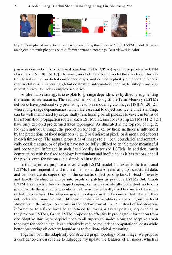
An alternative strategy is to exploit long-range dependencies by directly augmentingthe intermediate features. The multi-dimensional Long Short-Term Memory (LSTM)networks have produced very promising results in modeling 2D images [18][19][20][21],where long-range dependencies, which are essential to object and scene understanding,can be well memorized by sequentially functioning on all pixels. However, in terms ofthe information propagation route in each LSTM unit, most of existing LSTMs [1] [2] [21]have only explored pre-defined fixed topologies. As illusrated in the top row of Fig. 2,for each individual image, the prediction for each pixel by those methods is influencedby the predictions of fixed neighbors (e.g., 2 or 8 adjacent pixels or diagonal neighbors)in each time-step. The natural properties of images (e.g., local boundaries and semanti-cally consistent groups of pixels) have not be fully utilized to enable more meaningfuland economical inference in such fixed locally factorized LSTMs. In addition, muchcomputation with the fixed topology is redundant and inefficient as it has to consider allthe pixels, even for the ones in a simple plain region.

In this paper, we propose a novel Graph LSTM model that extends the traditionalLSTMs from sequential and multi-dimensional data to general graph-structured data,and demonstrate its superiority on the semantic object parsing task. Instead of evenlyand fixedly dividing an image into pixels or patches as previous LSTMs did, GraphLSTM takes each arbitrary-shaped superpixel as a semantically consistent node of agraph, while the spatial neighborhood relations are naturally used to construct the undi-rected graph edges. The adaptive graph topology can thus be constructed where differ-ent nodes are connected with different numbers of neighbors, depending on the localstructures in the image. As shown in the bottom row of Fig. 2, instead of broadcastinginformation to a fixed local neighborhood following a fixed updating sequence as inthe previous LSTMs, Graph LSTM proposes to effectively propagate information fromone adaptive starting superpixel node to all superpixel nodes along the adaptive graphtopology for each image. It can effectively reduce redundant computational costs whilebetter preserving object/part boundaries to facilitate global reasoning.

Together with the adaptively constructed graph topology of an image, we proposea confidence-driven scheme to subsequently update the features of all nodes, which is

Semantic Object Parsing with Graph LSTM 3

Row LSTM Diagonal BiLSTM Local-Global LSTM Pixel-wise LSTM

Graph LSTM

Image

Superpixel map Graph topology

Starting node

Current node

Neighboring nodes

Fig. 2. The proposed Graph LSTM structure. 1) The top row shows the traditional pixel-wise LSTM structures, including Row LSTM [2], Diagonal BiLSTM [2] [1] and Local-GlobalLSTM [21]. 2) The bottom row illustrates the proposed Graph LSTM that is built upon the su-perpixel over-segmentation map for each image.

inspired by the recent visual attention models [22][23]. Previous LSTMs [1][2] oftensimply start at pre-defined pixel or patch locations and then proceed toward other pixelsor patches following a fixed updating route for different images. In contrast, we assumethat starting from a proper superpixel node and updating the nodes following a certaincontent-adaptive path can lead to a more flexible and reliable inference for global con-text modelling, where the visual characteristics of each image can be better captured.

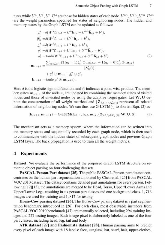
As shown in Fig. 3, the Graph LSTM, as an independent layer, can be easily ap-pended to the intermediate convolutional layers in a Fully Convolutional Neural Net-work [24] to strengthen visual feature learning by incorporating long-range contextualinformation. The hidden states represent the reinforced features, and the memory statesrecurrently encode the global structures.

Our contributions can be summarized in the following four aspects. 1) We pro-pose a novel Graph LSTM structure to extend the traditional LSTMs from sequentialand multi-dimensional data to general graph-structured data, which effectively exploitsglobal context by following an adaptive graph topology derived from the content ofeach image. 2) We propose a confidence-driven scheme to select the starting node andsequentially update all nodes, which facilitates the flexible inference while preservingthe visual characteristics of each image. 3) In each Graph LSTM unit, different forgetgates for the neighboring nodes are learned to dynamically incorporate the local con-textual interactions in accordance with their semantic relations. 4) We apply the pro-posed Graph LSTM in semantic object parsing, and demonstrate its superiority throughcomprehensive comparisons on four challenging semantic object parsing datasets (i.e.,PASCAL-Person-Part dataset [25], Horse-Cow parsing dataset [26], ATR dataset [27]and Fashionista dataset [28]).


Deep convnet

Graph LSTM

+ Graph LSTM +

Convolution

Adaptive node updating sequence

Confidence map

Convolution Confidence map

Residual connection Residual connection

Input

Parsing Result

Superpixel map

1 1

1 1

Fig. 3. Illustration of the proposed network architecture for semantic object parsing.

2 Related Work

LSTM on Image Processing: Recurrent neural networks have been first introducedto address the sequential prediction tasks [29] [30] [31], and then extended to multi-dimensional image processing tasks [18] [19].Benefiting from the long-range memo-rization of LSTM networks, they can obtain considerably larger dependency fields bysequentially performing LSTM units on all pixels, compared to the local convolutionalfilters. Nevertheless, in each LSTM unit, the prediction of each pixel is affected by afixed factorization (e.g., 2 or 8 neighboring pixels [1][32][21][33] or diagonal neigh-borhood [2][19]), where diverse natural visual correlations (e.g., local boundaries andhomogeneous regions) have not been considered. Meanwhile, the computation is verycostly and redundant due to the sequential computation on all pixels. Tree-LSTM [34]introduces the structure with tree-structured topologies for predicting semantic repre-sentations of sentences. Compared to Tree-LSTM, Graph LSTM is more natural andgeneral for 2D image processing with arbitrary graph topologies and adaptive updatingschemes.Semantic Object Parsing: There has been increasing research interest on the seman-tic object parsing problem including the general object parsing [26][16][35][25][36],person part segmentation [13][12] and human parsing [28][37][38][39][40][41][42].To capture the rich structure information based on the advanced CNN architecture,one common way is the combination of CNNs and CRFs [15][10][43][16], where theCNN outputs are treated as unary potentials while CRF further incorporates pairwise orhigher order factors. Instead of learning features only from local convolutional kernelsas in these previous methods, we incorporate the global context by the novel GraphLSTM structure to capture long-distance dependencies on the superpixels. The depen-dency field of Graph LSTM can effectively cover the entire image context.

3 The Proposed Graph LSTM

We take semantic object parsing as its application scenario, which aims to generatepixel-wise semantic part segmentation for each image. Fig. 3 illustrates the designed


network architecture based on Graph LSTM. The input image first passes through astack of convolutional layers to generate the convolutional feature maps.The proposedGraph LSTM takes the convolutional features and the adaptively specified node updat-ing sequence for each image as the input, and then efficiently propagates the aggregatedcontextual information towards all nodes, leading to enhanced visual features and betterparsing results. To both increase convergence speed and propagate signals more directlythrough the network, we deploy residual connections [44] after one Graph LSTM layerto generate the input features of the next Graph LSTM layer. Note that residual connec-tions are performed to generate the element-wise input features for each layer, whichwould not destroy the computed graph topology. After that, several 1 × 1 convolutionfilters are employed to produce the final parsing results. The following subsections willdescribe the main innovations inside Graph LSTM, including the graph constructionand the Graph LSTM structure.

3.1 Graph Construction

The graph is constructed on superpixels that are obtained through image over-segmentationusing SLIC [45]1. Note that, after several convolutional layers, the feature maps of eachimage have been down-sampled. Therefore, in order to use the superpixel map for graphconstruction in each Graph LSTM layer, one needs to upsample the feature maps intothe original size of the input image.

The superpixel graph G for each image is then constructed by connecting a setof graph nodes {vi}Ni=1 via the graph edges {Eij}. Each graph node vi represents asuperpixel and each graph edge Eij only connects two spatially neighboring superpixelnodes. The input features of each graph node vi are denoted as fi ∈ Rd, where dis the feature dimension. The feature fi is computed by averaging the features of allthe pixels belonging to the same superpixel node vi. As shown in Fig. 3, the inputstates of the first Graph LSTM layer come from the previous convolutional featuremaps. For the subsequent Graph LSTM layers, the input states are generated after theresidual connections [44] for the input features and the updated hidden states by theprevious Graph LSTM layer. To make sure that the number of the input states for thefirst Graph LSTM layer is compatible with that of the following layers and that theresidual connections can be applied, the dimensions of hidden and memory states in allGraph LSTM layers are set the same as the feature dimension of the last convolutionallayer before the first Graph LSTM layer.

3.2 Graph LSTM

Confidence-driven Scheme. The node updating scheme is more important yet morechallenging in Graph LSTM than the ones in traditional LSTMs [2][1] due to its adap-tive graph topology. To enable better global reasoning, Graph LSTM specifies the adap-tive starting node and node updating sequence for the information propagation of eachimage. Given the constructed undirected graph G, we extensively tried several schemes

1 Other over-segmentation methods such as entropy rate-based approach [41] could also be used,and we did not observe much difference in the final results in our experiments.


to update all nodes in a graph in the experiments, including the Breadth-First Search(BFS), Depth-First Search (DFS) and Confidence-Driven Search (CDS). We find thatthe CDS achieves better performance. Specifically, as illustrated in Fig. 3, given the topconvolutional feature maps, the 1 × 1 convolutional filters can be used to generate theinitial confidence maps with regard to each semantic label. Then the confidence of eachsuperpixel for each label is computed by averaging the confidences of its contained pix-els, and the label with highest confidence could be assigned to the superpixel. Amongall the foreground superpixels (i.e., assigned to any semantic part label), the node up-dating sequence can be determined by ranking all the superpixel nodes according to theconfidences of their assigned labels.

During updating, the (t + 1)-th Graph LSTM layer determines the current statesof each node vi that comprises the hidden states hi,t+1 ∈ Rd and memory statesmi,t+1 ∈ Rd of each node. Each node is influenced by its previous states and the statesof neighboring graph nodes as well in order to propagate information to the whole im-age. Thus the inputs to Graph LSTM units consist of the input states fi,t+1 of the nodevi, its previous hidden states hi,t and memory states mi,t, and the hidden and memorystates of its neighboring nodes vj , j ∈ NG(i).

Averaged Hidden States for Neighboring Nodes. Note that with an adaptive up-dating scheme, when operating on a specific node in each Graph LSTM layer, someof its neighboring nodes have already been updated while others may have not. Wetherefore use a visit flag qj to indicate whether the graph node vj has been updated,where qj is set as 1 if updated, and otherwise 0. We then use the updated hidden stateshj,t+1 for the visited nodes, i.e., qj = 1 and the previous states hj,t for the unvisitednodes. The 1(·) is an indicator function. Note that the nodes in the graph may have anarbitrary number of neighboring nodes. Let |NG(i)| denote the number of neighboringgraph nodes. To obtain a fixed feature dimension for the inputs of the Graph LSTM unitduring network training, the hidden states hi,t used for computing the LSTM gates ofthe node vi are obtained by averaging the hidden states of neighboring nodes, computedas:

hi,t =

∑j∈NG(i)(1(qj = 1)hj,t+1 + 1(qj = 0)hj,t)

|NG(i)|. (1)

Adaptive Forget Gates. Note that unlike the traditional LSTMs [1][46], the GraphLSTM specifies different forget gates for different neighboring nodes by functioningthe input states of the current node with their hidden states, defined as gfij , j ∈ NG(i).It results in the different influences of neighboring nodes on the updated memory statesmi,t+1 and hidden states hi,t+1. The memory states of each neighboring node are alsoutilized to update the memory states mi,t+1 of the current node. The shared weightmetrics Ufn for all nodes are learned to guarantee the spatial transformation invarianceand enable the learning with various neighbors. The intuition is that each pair of neigh-boring superpixels may be endowed with distinguished semantic correlations comparedto other pairs.

Graph LSTM Unit. The Graph LSTM consists of four gates: the input gate gu, theforget gate gf , the adaptive forget gate gf , the memory gate gc and the output gate go.The Wu,W f ,W c,W o are the recurrent gate weight matrices specified for input fea-


tures while Uu, Uf , U c, Uo are those for hidden states of each node. Uun, Ufn, U cn, Uon

are the weight parameters specified for states of neighboring nodes. The hidden andmemory states by the Graph LSTM can be updated as follows:

gui =δ(Wufi,t+1 + Uuhi,t + Uunhi,t + bu),

gfij =δ(W f fi,t+1 + Ufnhj,t + bf ),

gfi =δ(W f fi,t+1 + Ufhi,t + bf ),

goi =δ(W ofi,t+1 + Uohi,t + Uonhi,t + bo),

gci =tanh(W cfi,t+1 + Uchi,t + Ucnhi,t + bc),

mi,t+1 =

∑j∈NG(i)(1(qj = 1)gfij ⊙mj,t+1 + 1(qj = 0)gfij ⊙mj,t)

|NG(i)|+ gfi ⊙mi,t + gui ⊙ gci ,

hi,t+1 =tanh(goi ⊙mi,t+1).

(2)

Here δ is the logistic sigmoid function, and ⊙ indicates a point-wise product. The mem-ory states mi,t+1 of the node vi are updated by combining the memory states of visitednodes and those of unvisited nodes by using the adaptive forget gates. Let W,U de-note the concatenation of all weight matrices and {Zj,t}j∈NG(i) represent all relatedinformation of neighboring nodes. We can thus use G-LSTM(·) to shorten Eqn. (2) as

(hi,t+1,mi,t+1) = G-LSTM(fi,t+1,hi,t,mi,t, {Zj,t}j∈NG(i),W,U,G). (3)

The mechanism acts as a memory system, where the information can be written intothe memory states and sequentially recorded by each graph node, which is then usedto communicate with the hidden states of subsequent graph nodes and previous GraphLSTM layer. The back propagation is used to train all the weight metrics.

4 Experiments

Dataset: We evaluate the performance of the proposed Graph LSTM structure on se-mantic object parsing on four challenging datasets.

PASCAL-Person-Part dataset [25]. The public PASCAL-Person-part dataset con-centrates on the human part segmentation annotated by Chen et al. [25] from PASCALVOC 2010 dataset. The dataset contains detailed part annotations for every person. Fol-lowing [12][13], the annotations are merged to be Head, Torso, Upper/Lower Arms andUpper/Lower Legs, resulting in six person part classes and one background class. 1, 716images are used for training and 1, 817 for testing.

Horse-Cow parsing dataset [26]. The Horse-Cow parsing dataset is a part segmen-tation benchmark introduced in [26]. For each class, most observable instances fromPASCAL VOC 2010 benchmark [47] are manually selected, including 294 training im-ages and 227 testing images. Each image pixel is elaborately labeled as one of the fourpart classes, including head, leg, tail and body.

ATR dataset [27] and Fashionista dataset [28]. Human parsing aims to predictevery pixel of each image with 18 labels: face, sunglass, hat, scarf, hair, upper-clothes,


Table 1. Comparison of object parsing performance with four state-of-the-art methods over thePASCAL-Person-Part dataset [26].

Method head torso u-arms l-arms u-legs l-legs Bkg Avg

DeepLab-LargeFOV [15] 78.09 54.02 37.29 36.85 33.73 29.61 92.85 51.78HAZN [12] 80.79 59.11 43.05 42.76 38.99 34.46 93.59 56.11

Attention [13] - - - - - - - 56.39LG-LSTM [21] 82.72 60.99 45.40 47.76 42.33 37.96 88.63 57.97

Graph LSTM 82.69 62.68 46.88 47.71 45.66 40.93 94.59 60.16

left-arm, right-arm, belt, pants, left-leg, right-leg, skirt, left-shoe, right-shoe, bag, dressand null. Originally, 7,700 images are included in the ATR dataset [27], with 6,000 fortraining, 1,000 for testing and 700 for validation. 10,000 real-world human pictures arefurther collected by [42] to cover images with more challenging poses, occlusion andclothes variations. We follow the training and testing settings used in [42].Evaluation metric: The standard intersection over union (IOU) criterion and pixel-wise accuracy are adopted for evaluation on PASCAL-Person-Part dataset and Horse-Cow parsing dataset, following [26][36][13]. We use the same evaluation metrics asin [37][27][42] for evaluation on two human parsing datasets, including accuracy, aver-age precision, average recall, and average F-1 score.Network architecture: For fair comparison with [16][12][13], our network is basedon the publicly available model, “DeepLab-CRF-LargeFOV” [15] for the PASCAL-Person-Part and Horse-Cow parsing dataset, which slightly modifies VGG-16 net [48]to FCN [24]. For fair comparing with [21][42] on two human parsing datasets, thebasic “Co-CNN” structure proposed in [42] is utilized due to its leading accuracy. Ournetworks based on “Co-CNN” are trained from the scratch following the same settingin [42].Training: We use the same data augmentation techniques for the object part segmenta-tion and human parsing as in [16] and [42], respectively. The scale of the input image isfixed as 321× 321 for training networks based on “DeepLab-CRF-LargeFOV”. Basedon “Co-CNN”, the input image is rescaled to 150 × 100 as in [42]. We use the SLICover-segmentation method [45] to generate averagely 1,000 superpixels for each image.Two training steps are employed to train the networks. First, we train the convolutionallayer with 1× 1 filters to generate initial confidence maps that are used to produce thestarting node and the update sequence for all nodes in Graph LSTM. Then, the wholenetwork is fine-tuned based on the pretrained model to produce final parsing results. Ineach step, the learning rate of the newly added layers, including Graph LSTM layers andconvolutional layers is initialized as 0.001 and that of other previously learned layers, isinitialized as 0.0001. All weight matrices used in the Graph LSTM units are randomlyinitialized from a uniform distribution of [-0.1, 0.1]. The Graph LSTM predicts the hid-den and memory states with the same dimension as in the previous convolutional layers.We only use two Graph LSTM layers for all models since only slight improvements areobserved by using more Graph LSTM layers, which also consumes more computationresources. We fine-tune the networks on “DeepLab-CRF-LargeFOV” for roughly 60epochs and it takes about 1 day. For training based on “Co-CNN” from scratch, it takes


Table 2. Comparison of object parsing performance with five state-of-the-art methods over theHorse-Cow object parsing dataset [26].

HorseMethod Bkg head body leg tail Fg IOU Pix.Acc

SPS [26] 79.14 47.64 69.74 38.85 - 68.63 - 81.45HC [36] 85.71 57.30 77.88 51.93 37.10 78.84 61.98 87.18

Joint [16] 87.34 60.02 77.52 58.35 51.88 80.70 65.02 88.49LG-LSTM [21] 89.64 66.89 84.20 60.88 42.06 82.50 68.73 90.92

HAZN [12] 90.87 70.73 84.45 63.59 51.16 - 72.16 -

Graph LSTM 91.73 72.89 86.34 69.04 53.76 87.51 74.75 92.76

CowMethod Bkg head body leg tail Fg IOU Pix.Acc

SPS [26] 78.00 40.55 61.65 36.32 - 71.98 - 78.97HC [36] 81.86 55.18 72.75 42.03 11.04 77.04 52.57 84.43

Joint [16] 85.68 58.04 76.04 51.12 15.00 82.63 57.18 87.00LG-LSTM [21] 89.71 68.43 82.47 53.93 19.41 85.41 62.79 90.43

HAZN [12] 90.66 75.10 83.30 57.17 28.46 - 66.94 -

Graph LSTM 91.54 73.88 85.92 63.67 35.22 88.42 70.05 92.43

Table 3. Comparison of human parsing performance with seven state-of-the-art methods whenevaluating on ATR dataset [27].

Method Acc. F.g. acc. Avg. prec. Avg. recall Avg. F-1 score

Yamaguchi et al. [28] 84.38 55.59 37.54 51.05 41.80PaperDoll [37] 88.96 62.18 52.75 49.43 44.76M-CNN [41] 89.57 73.98 64.56 65.17 62.81

ATR [27] 91.11 71.04 71.69 60.25 64.38Co-CNN [42] 95.23 80.90 81.55 74.42 76.95

Co-CNN (more) [42] 96.02 83.57 84.95 77.66 80.14LG-LSTM [21] 96.18 84.79 84.64 79.43 80.97

LG-LSTM (more) [21] 96.85 87.35 85.94 82.79 84.12CRFasRNN (more) [10] 96.34 85.10 84.00 80.70 82.08

Graph LSTM 97.60 91.42 84.74 83.28 83.76Graph LSTM (more) 97.99 93.06 88.81 87.80 88.20

about 4-5 days. In the testing stage, one image takes 0.5 second on average except forthe superpixel extraction step.

4.1 Results and Comparisons

We compare the proposed Graph LSTM structure with several state-of-the-art methodson four public datasets.

PASCAL-Person-Part dataset [26]: We report the results and the comparisonswith four recent state-of-the-art methods [15][12][13][21] in Table 1. The results of“DeepLab-LargeFOV” were originally reported in [12]. The proposed Graph LSTMstructure substantially outperforms these baselines in terms of average IoU metric. Inparticular, for the semantic parts with more likely confusions such as upper-arms andlower-arms, the Graph LSTM provides considerably better prediction than baselines,e.g., 4.95% and 6.67% higher over [12] for lower-arms and upper-legs, respectively.This superior performance achieved by Graph LSTM demonstrates the effectiveness ofexploiting global context to boost local prediction.


Table 4. Comparison of human parsing performance with five state-of-the-art methods on the testimages of Fashionista [28].

Method Acc. F.g. acc. Avg. prec. Avg. recall Avg. F-1 score

Yamaguchi et al. [28] 87.87 58.85 51.04 48.05 42.87PaperDoll [37] 89.98 65.66 54.87 51.16 46.80

ATR [27] 92.33 76.54 73.93 66.49 69.30Co-CNN [42] 96.08 84.71 82.98 77.78 79.37

Co-CNN (more) [42] 97.06 89.15 87.83 81.73 83.78LG-LSTM [21] 96.85 87.71 87.05 82.14 83.67

LG-LSTM (more) [21] 97.66 91.35 89.54 85.54 86.94

Graph LSTM 97.93 92.78 88.24 87.13 87.57Graph LSTM (more) 98.14 93.75 90.15 89.46 89.75

Table 5. Per-Class Comparison of F-1 scores with six state-of-the-art methods on ATR [27].

Method Hat Hair S-gls U-cloth Skirt Pants Dress Belt L-shoe R-shoe Face L-leg R-leg L-arm R-arm Bag Scarf

Yamaguchi et al. [28] 8.44 59.96 12.09 56.07 17.57 55.42 40.94 14.68 38.24 38.33 72.10 58.52 57.03 45.33 46.65 24.53 11.43PaperDoll [37] 1.72 63.58 0.23 71.87 40.20 69.35 59.49 16.94 45.79 44.47 61.63 52.19 55.60 45.23 46.75 30.52 2.95M-CNN [41] 80.77 65.31 35.55 72.58 77.86 70.71 81.44 38.45 53.87 48.57 72.78 63.25 68.24 57.40 51.12 57.87 43.38

ATR [27] 77.97 68.18 29.20 79.39 80.36 79.77 82.02 22.88 53.51 50.26 74.71 69.07 71.69 53.79 58.57 53.66 57.07Co-CNN [42] 72.07 86.33 72.81 85.72 70.82 83.05 69.95 37.66 76.48 76.80 89.02 85.49 85.23 84.16 84.04 81.51 44.94

Co-CNN more [42] 75.88 89.97 81.26 87.38 71.94 84.89 71.03 40.14 81.43 81.49 92.73 88.77 88.48 89.00 88.71 83.81 46.24LG-LSTM (more) [21] 81.13 90.94 81.07 88.97 80.91 91.47 77.18 60.32 83.40 83.65 93.67 92.27 92.41 90.20 90.13 85.78 51.09

Graph LSTM (more) 85.30 90.47 72.77 95.11 97.31 96.58 96.43 68.55 85.27 84.35 92.70 91.13 93.17 91.20 81.00 90.83 66.09

Horse-Cow Parsing dataset [26]: Table 2 shows the comparison results with fivestate-of-the-art methods on the overall metrics. The proposed Graph LSTM gives ahuge boost in average IOU. For example, Graph LSTM achieves 70.05%, 7.26% bet-ter than LG-LSTM [21] and 3.11% better than HAZN [12] for the cow class. Largeimprovement, i.e. 2.59% increase by Graph LSTM in IOU over the best performingstate-of-the-art method, can also be observed from the comparisons on horse class.

ATR dataset [27]: Table 3 and Table 5 report the comparison performance withseven state-of-the-arts on overall metrics and F-1 scores of individual semantic labels,respectively. The proposed Graph LSTM can significantly outperform these baselines,particularly, 83.76% vs 76.95% of Co-CNN [42] and 80.97% of LG-LSTM [21] interms of average F-1 score. Following [42], we also take the additional 10,000 imagesin [42] as extra training images and report the results as “Graph LSTM (more)”. The“Graph LSTM (more)” can also improve the average F-1 score by 4.08% over “LG-LSTM (more)”. We show the F-1 score for each label in Table 5. Generally, our GraphLSTM shows much higher performance than other baselines. In addition, our “GraphLSTM (more)” significantly outperforms “CRFasRNN (more)” [10], verifying the su-periority of Graph LSTM over the pair-wise terms in CRF in capturing global context.The results of “CRFasRNN (more)” [10] are obtained by training the network usingtheir public code.

Fashionista dataset [28]: Table 4 gives the comparison results on the Fashionistadataset. Following [27], we only report the performance by training on the same largeATR dataset [27] and then testing on the 229 images of the Fashionista dataset. OurGraph LSTM architecture can substantially outperform the baselines by a large gain.


Table 6. Performance comparisons of using different LSTM structures and taking the superpixelsmoothing as the post-processing step when evaluating on PASCAL-Person-Part dataset.


Grid LSTM [1] 81.85 58.85 43.10 46.87 40.07 34.59 85.97 55.90Row LSTM [2] 82.60 60.13 44.29 47.22 40.83 35.51 87.07 56.80

Diagonal BiLSTM [2] 82.67 60.64 45.02 47.59 41.95 37.32 88.16 57.62LG-LSTM [21] 82.72 60.99 45.40 47.76 42.33 37.96 88.63 57.97

Diagonal BiLSTM [2] + superpixel smoothing 82.91 61.34 46.01 48.07 42.56 37.91 89.21 58.29LG-LSTM [21] + superpixel smoothing 82.98 61.58 46.27 48.08 42.94 38.55 89.66 58.58

Graph LSTM 82.69 62.68 46.88 47.71 45.66 40.93 94.59 60.16

Table 7. Performance comparisons with different node updating schemes when evaluating onPASCAL-Person-Part dataset.


BFS (location) 83.00 61.63 46.18 48.01 44.09 38.71 93.82 58.63BFS (confidence) 82.97 62.20 46.70 48.00 44.02 39.00 90.86 59.11

DFS (location) 82.85 61.25 45.89 48.02 42.50 38.10 89.04 58.23DFS (confidence) 82.89 62.31 46.76 48.04 44.24 39.07 91.18 59.21

Graph LSTM (confidence-driven) 82.69 62.68 46.88 47.71 45.66 40.93 94.59 60.16

4.2 Discussions

Graph LSTM vs locally fixed factorized LSTM. To show the superiority of the GraphLSTM compared to previous locally fixed factorized LSTM [2][21][1], Table 6 givesthe performance comparison among different LSTM structures. These variants use thesame network architecture and only replace the Graph LSTM layer with the traditionalfixedly factorized LSTM layer, including Row LSTM [2], Diagonal BiLSTM [2], LG-LSTM [21] and Grid LSTM [1]. The experimented Grid LSTM [1] is a simplified ver-sion of Diagnocal BiLSTM [2] where only the top and left pixels are considered. Theirbasic structures are presented in Fig. 2. It can be observed that using richer local con-texts (i.e., number of neighbors) to update the states of each pixel can lead to betterparsing performance. In average, there are six neighboring nodes for each superpixelnode in the constructed graph topologies in Graph LSTM. Although the LG-LSTM [21]has employed eight neighboring pixels to guide local prediction, its performance is stillworse than our Graph LSTM.

Graph LSTM vs superpixel smoothing. In Table 6, we further demonstrate thatthe performance gain by Graph LSTM is not just from using more accurate bound-ary information provided by superpixels. The superpixel smoothing can be used asa post-processing step to refine confidence maps by previous LSTMs. By comparing“Diagonal BiLSTM [2] + superpixel smoothing” and “LG-LSTM [21] + superpixelsmoothing” with our “Graph LSTM”, we can find that the Graph LSTM can still bringmore performance gain benefiting from its advanced information propagation based onthe graph-structured representation.

Node updating scheme. Different node updating schemes to update the states of allnodes are further investigated in Table 7. The Breadth-first search (BFS) and Depth-firstsearch (DFS) are the traditional algorithms to search graph data structures. For one par-


Table 8. Performance comparisons of using the confidence-drive scheme based on confidenceson different foreground labels when evaluating on PASCAL-Person-Part dataset.

Foreground label head torso u-arms l-arms u-legs l-legs AvgAvg IoU 61.03 61.45 60.03 59.23 60.49 59.89 60.35

ent node, selecting different children nodes to first update may lead to different updatedhidden states for all nodes. Two ways of selecting first children nodes for updatingare thus evaluated: “BFS (location)” and “DFS (location)” choose the spatially left-most node among all children nodes to update first while “BFS (confidence)” and “DFS(confidence)” select the child node with maximal confidence on all foreground classes.We find that using our confidence-driven scheme can achieve better performance thanother alternative ones. The possible reason may be that the features of superpixel nodeswith higher foreground confidences embed more accurate semantic meanings and thuslead to more reliable global reasoning.

Note that we use the ranking of confidences on all foreground classes to generatethe node updating scheme. In Table 8, we extensively test the performance of usingthe initial confidence maps of different foreground labels to produce the node updat-ing sequence. In average, only slight performance differences are observed when usingthe confidences of different foreground labels. In particular, using the confidences of“head” and “torso” leads to improved performance over using those of all foregroundclasses, i.e., 61.03% and 61.45% vs 60.16%. It is possible because the segmentation ofhead/torso are more reliable in the person parsing case, which further verifies that thereliability of nodes in the updating order is important. It is difficult to determine the bestsemantic label for each task, hence we just use the one over all the foreground labelsfor simplicity and efficiency in implementation.

Adaptive forget gates. In Graph LSTM, adaptive forget gates are adopted to treatthe local contexts from different neighbors differently. The superiority of using adap-tive forget gates can be verified in Table 9. “Identical forget gates” shows the results oflearning identical forget gates for all neighbors and simultaneously ignoring the mem-ory states of neighboring nodes. Thus in “Identical forget gates”, the gfi and mi,t+1 inEqn. (2) can be simply computed as

gfi =δ(W f fi,t+1 + Ufhi,t + Ufnhi,t + bf ),

mi,t+1 =gfi ⊙mi,t + gui ⊙ gci .(4)

It can be observed that learning adaptive forgets gates in Graph LSTM shows betterperformance over learning identical forget gates for all neighbors on the object parsingtask, as diverse semantic correlations with local context can be considered and treateddifferently during the node updating. Compared to Eqn. (4), no extra parameters isbrought to specify adaptive forget gates due to the usage of the shared parameters Ufn

in Eqn. (2).Superpixel number. The drawback of using superpixels is that superpixels may in-

troduce quantization errors whenever pixels within one superpixel have different ground


Table 9. Comparisons of parsing performance by the version with or without learning adaptiveforget gates for different neighboring nodes when evaluating on PASCAL-Person-Part dataset.


Identical forget gates 82.89 62.31 46.76 48.04 44.24 39.07 91.18 59.21

Graph LSTM (dynamic forget gates) 82.69 62.68 46.88 47.71 45.66 40.93 94.59 60.16

0 500 1000 1500

40

50

60

70

80

90

100

Avg. Number of Superpixels

Perf

orm

ance

(%)

Avg IoU (PASCAL−Person−Part)Avg F−1 score (ATR)

Fig. 4. Performance comparisons with six averaged numbers of superpixels when evaluating onPASCAL-Person-Part and ATR datasets, including 250, 500, 750, 1000, 1250, 1500 .

truth labels. We thus evaluate the performance of using different average numbers of su-perpixels to construct the graph structure. As shown in Fig. 4, there are slight improve-ments when using over 1,000 superpixels. We thus use averagely 1,000 superpixels foreach image in all our experiments.

Failure cases

Input Deeplab-LargeFov Graph LSTM Input Deeplab-LargeFov Graph LSTM

Head

Upper Arms

Torso

Upper Legs

Lower Legs

Lower Arms

Fig. 5. Comparison of parsing results of our Graph LSTM and the baseline “DeepLab-LargeFov”and some failure cases by our Graph LSTM on PASCAL-Person-Part.

Residual connections. Residual connections were first proposed in [44] to bettertrain very deep convolutional layers. The version in which the residual connections areeliminated achieves 59.12% in terms of Avg IoU on PASCAL-Person-Part dataset. Itdemonstrates that residual connections between Graph LSTM layers can also help boostthe performance, i.e., 60.16% vs 59.12%. Note that our Graph LSTM version withoutusing residual connections is still significantly better than all baselines in Table 1.


4.3 More Visual Comparison and Failure cases

The qualitative comparisons of parsing results on PASCAL-Person-Part and ATR datasetare visualized in Fig. 5 and Fig. 6, respectively. In general, our Graph-LSTM outputsmore reasonable results for confusing labels by effectively exploiting global context toassist the local prediction. We also show some failure cases on each dataset.

Input LG-LSTM Graph-LSTM Input LG-LSTM Graph-LSTM Input LG-LSTM Graph-LSTM

Failure cases

Fig. 6. Parsing result comparisons of our Graph LSTM and the LG-LSTM [21] and some failurecases by our Graph LSTM on ATR dataset.

5 Conclusion and Future Work

In this work, we proposed a novel Graph LSTM network to address the fundamental se-mantic object parsing task. Our Graph LSTM generalizes the existing LSTMs into thegraph-structured data. The adaptive graph topology for each image is constructed byconnecting the arbitrary-shaped superpixels nodes via their spatial neighborhood con-nections. The confidence-driven scheme is used to adaptively select the starting nodeand determine the node updating sequence. The Graph LSTM can thus sequentially up-date the states of all nodes. Comprehensive evaluations on four public semantic objectparsing datasets well demonstrate the significant superiority of our graph LSTM. In fu-ture, we will explore how to dynamically adjust the graph structure to directly producethe semantic masks according to the connected superpixel nodes.

Acknowledgement This work was supported in part by State Key Development Pro-gram under Grant 2016YFB1001000 and Special Program for Applied Research onSuper Computation of the NSFC-Guangdong Joint Fund (the second phase). The workof Jiashi Feng was partially supported by National University of Singapore startup grantR-263-000-C08-133 and Ministry of Education of Singapore AcRF Tier One grant R-263-000-C21-112.


References

1. Kalchbrenner, N., Danihelka, I., Graves, A.: Grid long short-term memory. In: ICLR. (2016)2. van den Oord, A., Kalchbrenner, N., Kavukcuoglu, K.: Pixel recurrent neural networks. In:

ICML. (2016)3. Zhang, H., Kim, G., Xing, E.P.: Dynamic topic modeling for monitoring market competition

from online text and image data. In: ACM SIGKDD, ACM (2015) 1425–14344. Zhang, H., Hu, Z., Wei, J., Xie, P., Kim, G., Ho, Q., Xing, E.: Poseidon: A system architecture

for efficient gpu-based deep learning on multiple machines. arXiv preprint arXiv:1512.06216(2015)

5. Zhao, R., Ouyang, W., Wang, X.: Unsupervised salience learning for person re-identification.In: CVPR. (2013) 3586–3593

6. Wang, Y., Tran, D., Liao, Z., Forsyth, D.: Discriminative hierarchical part-based models forhuman parsing and action recognition. JMLR 13(1) (2012) 3075–3102

7. Gan, C., Wang, N., Yang, Y., Yeung, D.Y., Hauptmann, A.G.: Devnet: A deep event networkfor multimedia event detection and evidence recounting. In: CVPR. (2015) 2568–2577

8. Gan, C., Lin, M., Yang, Y., de Melo, G., Hauptmann, A.G.: Concepts not alone: Exploringpairwise relationships for zero-shot video activity recognition. In: AAAI. (2016)

9. Liang, X., Wei, Y., Shen, X., Yang, J., Lin, L., Yan, S.: Proposal-free network for instance-level object segmentation. arXiv preprint arXiv:1509.02636 (2015)

10. Zheng, S., Jayasumana, S., Romera-Paredes, B., Vineet, V., Su, Z., Du, D., Huang, C., Torr,P.: Conditional random fields as recurrent neural networks. In: ICCV. (2015)

11. Liang, X., Liu, S., Wei, Y., Liu, L., Lin, L., Yan, S.: Towards computational baby learning:A weakly-supervised approach for object detection. In: ICCV. (2015) 999–1007

12. Xia, F., Wang, P., Chen, L.C., Yuille, A.L.: Zoom better to see clearer: Huamn part segmen-tation with auto zoom net. In: ECCV. (2016)

13. Chen, L.C., Yang, Y., Wang, J., Xu, W., Yuille, A.L.: Attention to scale: Scale-aware seman-tic image segmentation. In: CVPR. (2016)

14. Eigen, D., Fergus, R.: Predicting depth, surface normals and semantic labels with a commonmulti-scale convolutional architecture. In: ICCV. (2015)

15. Chen, L.C., Papandreou, G., Kokkinos, I., Murphy, K., Yuille, A.L.: Semantic Image Seg-mentation with Deep Convolutional Nets and Fully Connected CRFs. In ICLR (2015)

16. Wang, P., Shen, X., Lin, Z., Cohen, S., Price, B., Yuille, A.: Joint object and part segmenta-tion using deep learned potentials. In: ICCV. (2015)

17. Gadde, R., Jampani, V., Kiefel, M., Gehler, P.V.: Superpixel convolutional networks usingbilateral inceptions. In: ICLR. (2016)

18. Byeon, W., Liwicki, M., Breuel, T.M.: Texture classification using 2d lstm networks. In:ICPR. (2014) 1144–1149

19. Theis, L., Bethge, M.: Generative image modeling using spatial lstms. In: NIPS. (2015)20. Byeon, W., Breuel, T.M., Raue, F., Liwicki, M.: Scene Labeling with LSTM Recurrent

Neural Networks. In: CVPR. (2015) 3547–355521. Liang, X., Shen, X., Xiang, D., Feng, J., Lin, L., Yan, S.: Semantic object parsing with

local-global long short-term memory. In: CVPR. (2016)22. Sharma, S., Kiros, R., Salakhutdinov, R.: Action recognition using visual attention. arXiv

preprint arXiv:1511.04119 (2015)23. Mnih, V., Heess, N., Graves, A., et al.: Recurrent models of visual attention. In: Advances

in Neural Information Processing Systems. (2014) 2204–221224. Long, J., Shelhamer, E., Darrell, T.: Fully convolutional networks for semantic segmentation.

In: CVPR. (2015)


25. Chen, X., Mottaghi, R., Liu, X., Fidler, S., Urtasun, R., et al.: Detect what you can: Detectingand representing objects using holistic models and body parts. In: CVPR. (2014) 1979–1986

26. Wang, J., Yuille, A.: Semantic part segmentation using compositional model combiningshape and appearance. In: CVPR. (2015)

27. Liang, X., Liu, S., Shen, X., Yang, J., Liu, L., Dong, J., Lin, L., Yan, S.: Deep human parsingwith active template regression. TPAMI (2015)

28. Yamaguchi, K., Kiapour, M., Ortiz, L., Berg, T.: Parsing clothing in fashion photographs.In: CVPR. (2012)

29. Graves, A., Schmidhuber, J.: Offline handwriting recognition with multidimensional recur-rent neural networks. In: NIPS. (2009) 545–552

30. Sutskever, I., Vinyals, O., Le, Q.V.: Sequence to sequence learning with neural networks. In:NIPS. (2014) 3104–3112

31. Xu, K., Ba, J., Kiros, R., Cho, K., Courville, A.C., Salakhutdinov, R., Zemel, R.S., Bengio,Y.: Show, attend and tell: Neural image caption generation with visual attention. In: ICML.(2015) 2048–2057

32. Graves, A., Fernandez, S., Schmidhuber, J.: Multi-dimensional recurrent neural networks.In: ICANN. (2007)

33. Stollenga, M.F., Byeon, W., Liwicki, M., Schmidhuber, J.: Parallel multi-dimensionallstm, with application to fast biomedical volumetric image segmentation. arXiv preprintarXiv:1506.07452 (2015)

34. Tai, K.S., Socher, R., Manning, C.D.: Improved semantic representations from tree-structured long short-term memory networks. arXiv preprint arXiv:1503.00075 (2015)

35. Lu, W., Lian, X., Yuille, A.: Parsing semantic parts of cars using graphical models andsegment appearance consistency. In: BMVC. (2014)

36. Hariharan, B., Arbelaez, P., Girshick, R., Malik, J.: Hypercolumns for object segmentationand fine-grained localization. In: CVPR. 447–456

37. Yamaguchi, K., Kiapour, M., Berg, T.: Paper doll parsing: Retrieving similar styles to parseclothing items. In: ICCV. (2013)

38. Dong, J., Chen, Q., Xia, W., Huang, Z., Yan, S.: A deformable mixture parsing model withparselets. In: ICCV. (2013)

39. Wang, N., Ai, H.: Who blocks who: Simultaneous clothing segmentation for grouping im-ages. In: ICCV. (2011)

40. Simo-Serra, E., Fidler, S., Moreno-Noguer, F., Urtasun, R.: A High Performance CRF Modelfor Clothes Parsing. In: ACCV. (2014)

41. Liu, S., Liang, X., Liu, L., Shen, X., Yang, J., Xu, C., Lin, L., Cao, X., Yan, S.: Matching-CNN Meets KNN: Quasi-Parametric Human Parsing. In: CVPR. (2015)

42. Liang, X., Xu, C., Shen, X., Yang, J., Liu, S., Tang, J., Lin, L., Yan, S.: Human parsing withcontextualized convolutional neural network. In: ICCV. (2015)

43. Schwing, A.G., Urtasun, R.: Fully connected deep structured networks. arXiv preprintarXiv:1503.02351 (2015)

44. He, K., Zhang, X., Ren, S., Sun, J.: Deep residual learning for image recognition. In: CVPR.(2016)

45. Achanta, R., Shaji, A., Smith, K., Lucchi, A., Fua, P., Susstrunk, S.: Slic superpixels. Tech-nical report (2010)

46. Hochreiter, S., Schmidhuber, J.: Long short-term memory. Neural computation 9(8) (1997)1735–1780

47. Everingham, M., Van Gool, L., Williams, C.K., Winn, J., Zisserman, A.: The pascal visualobject classes challenge 2010 (voc2010) results (2010)

48. Simonyan, K., Zisserman, A.: Very deep convolutional networks for large-scale image recog-nition. arXiv preprint arXiv:1409.1556 (2014)

Documents

Semantic Object Parsing with Graph LSTMusers.eecs.northwestern.edu/~xsh835/assets/eccv2016... · 2016-08-22 · Semantic Object Parsing with Graph LSTM 3 RowLSTM Diagonal BiLSTM Local-Global