Semi-rational Models of Conditioning: The Case of Trial …dayan/papers/dawcourvday08.pdf · Semi-rational Models of Conditioning: The Case ... distinction between performance and

Chapter 19

Semi-rational Models ofConditioning: The Case of TrialOrder

Nathaniel D. Daw, Aaron C. Courville, andPeter DayanJune 15, 2007

1 IntroductionBayesian treatments of animal conditioning start from a generative model that speci-fies precisely a set of assumptions about the structure of the learning task. Optimalrules for learning are direct mathematical consequences of these assumptions. Interms of Marr’s (1982) levels of analyses, the main task at the computational levelwould therefore seem to be to understand and characterize the set of assumptionsfrom the observed behavior. However, a major problem with such Marrian analyses is that most Bayesian models for learning are presumptively untenable due to theirradically intractable computational demands.

This tension between what the observer should and what she can do relates toMarr’s (1982) distinction between the computational and algorithmic levels,Chomsky’s (1965) distinction between performance and competence, and Simon’s(1957) notion of bounded rationality. As all these examples suggest, we need not sim-ply abandon normative considerations in favor of unconstrained, cheap and cheerfulheuristics. Indeed, the evolutionary argument often taken to justify a normativeapproach (that organisms behaving rationally will enjoy higher fitness) in fact sug-gests that, in light of computational costs, evolution should favor those who can bestand most efficiently approximate rational computations.

In short, some irrational models are more rational than others, and it is these thatwe suggest should be found to model behavior and its neural substrates best. Here, insearch of such models, we look to the burgeoning and theoretically sophisticated fieldstudying approximations to exact Bayesian inference.

The major difficulty facing such analyses is distinguishing which characteristics ofobserved behavior relate to the underlying assumptions, and which to approxima-tions employed in bringing them to bear. This is particularly challenging since we donot know very much about how expensive computation is in the brain, and thereforethe potential tradeoff between costs and competence. As with all model selectionquestions, the short answer to the question of assumption versus approximation is, ofcourse, that we cannot tell for sure.

In fact, that assumption and approximation are difficult to distinguish is a particu-larly acute problem for theorists attempting to study normative considerations in

19-Charter&Oaksford-Chap19 11/5/07 11:22 AM Page 427

isolation, which motivates our attempt to study both together. In practice, we mayhope that credible candidates for both assumptions and approximations have differ-ent and rather specific qualitative fingerprints. In this chapter, we explore these ideasin the context of models of Pavlovian conditioning and prediction experiments inanimals and humans. In particular, we address the recent trenchant discussion of Kruschke (2006), who argued against pure Bayesian learning models in favor of aparticular heuristic treatment based on the effects of trial ordering in tasks such asbackward blocking (Lovibond et al., 2003; Shanks, 1985; Wasserman and Berglan,1998) and highlighting (Kruschke, 2003, 2006; Medin and Bettger, 1991). His ‘locallyBayesian’ model, while drawing on Bayesian methods, neither corresponds to exactinference nor is motivated or justified as an approximation to the ideal.

While we agree with Kruschke that features of the data suggest something short ofideal reasoning in the statistical models we consider, we differ in the substance of thealternative modeling frameworks that we employ. On our analysis, at the computa-tional level, effects of the ordering of trials bring up the issue of assumptions abouthow task contingencies change. The qualitative fingerprint here is recency – for mostcredible such models, recent trials will provide more information about the presentstate of affairs than distant trials. We show that some trial order effects emerge fromoptimal inference. For others, notably highlighting, which appears to be inconsistentwith recency, we consider the effects of inferential approximation. We show how primacy effects, as seen in highlighting, qualitatively characterize a number of simpli-fied inference schemes.

We start by describing the Kalman filter model of con ditioning (Dayan et al.,2000), which arises as the exact inference process associated with an analyticallytractable, but highly simplified, Bayesian model of change. We show that this modelleads to certain trial order effects, including those associated with backward blocking;we then consider inferential approximations in this framework and their implicationsfor trial ordering in highlighting. We conclude with a discussion of how approxima-tions might be explicitly balanced by reasoning about their accuracy.

2 Learning as Filtering

2.1 The Generative ModelConsider a prediction problem in which, on trial t, the subject observes a possiblymultidimensional stimulus xt and must predict an outcome rt. In a classical condi-tioning experiment, x might be a binary vector reporting which of a set of stimulisuch as tones and lights were present and r some continuously distributed amount offood subsequently delivered. (We denote possible stimuli as A, B, C and write a unitamount of food as R.) In this case, the animal’s prediction about r is of course meas-ured implicitly, e.g. through salivation. In a human experiment using, for instance,a medical cover story, x might report a set of foods (e.g.x=AC), with r being a binaryvariable reporting whether a patient developed an allergic reaction from eating them(e.g. r = R or 0).

We briefly review a familiar statistical approach to such a problem (e.g. Dayan andLong, 1998; Griffiths and Yuille, this volume). This begins by assuming a space of

SEMI-RATIONAL MODELS OF CONDITIONING: THE CASE OF TRIAL ORDER428


hypotheses about how the data (D, a sequence of x→r pairs) were generated. Suchhypotheses often take the form of a parameterized stochastic data generation process,which assigns probability P(D|q) to each possible data set D as a function of the (ini-tially unknown or uncertain) parameter settings q. Then, conditional on havingobserved some data (and on any prior beliefs about q), one can use Bayes’ rule todraw inferences about the posterior likelihood of the hypotheses (here, parameter set-tings),P(q |D). Finally, to choose how to act on a new trial T, with stimuli xT, the sub-ject can calculate the posterior distribution over rT using the likelihood-weightedaverage over the outcomes given the stimuli and each hypothesis:

(1)

The interpretive power of the approach rests on its normative, statistical foundation.Indeed, the whole procedure is optimal inference based on just the generative modeland priors, which collectively describe what is known (or at least assumed) about howthe data are generated.

The generative models of conditioning based on these principles typically split intotwo pieces. First, they assume that included in q is one or more sets of values wt thatgovern a distribution P(rt|xt,wt) over the output on trial t given the stimuli. Second,they assume something about the probabilistic relationship between the parameterswt and wt +1 associated with successive trials. The job of the subject, on this view, is toestimate the posterior distribution P(w|D) from past outcomes so as to predict futureoutcomes. We discuss the two pieces of the models in turn.

2.2 Parameterized Output DistributionOne standard assumption is that the outcome rt on trial t is drawn from a Gaussiandistribution:

(2)

Here, the weights wt specify the mean outcomes wtj expected in the presence of eachstimulus j individually, and s0 is the level of noise corrupting each trial. We typicallyassume that s0 is known, although it is formally (though not necessarily computa-tionally) easy to infer it too from the data.

There are various points to make about this formulation. First, note that Equation 2characterizes the outcome rt conditional on the input xt, rather than modeling theprobability of both variables jointly. In this sense it is not a full generative model forthe data D (which consist of both stimuli and outcomes). However, it suffices for thepresent purposes of asking how subjects perform the task of predicting an rt given an xt.We have elsewhere considered full joint models (Courville et al., 2003, 2004, 2006).

Second, in Equation 2, the mean of the net prediction is assumed to be a sum of thepredictions wtj associated with all those stimuli xtj present on trial t. This is ecologi-cally natural in some contexts, and is deeply linked to the Rescorla–Wagner (1972)model’s celebrated account of cue combination phenomena such as blocking andconditioned inhibition. However, there are other possibilities in which the stimuli are

P r w xT T T o tj tj oj

( | , , ) ,x w σ σ= ⋅⎛

⎝⎜

⎞

⎠⎟∑N 2

P r P r PT T T T( | , ) = d ( | , ) ( | )x xD Dq q q∫

LEARNING AS FILTERING 429


treated as competing predictors (rather than cooperating ones: Jacobs et al., 1991a,b).For instance, one alternative formulation is that of an additive mixture of Gaussians,which uses an extra vector of parameters ptŒq to capture the competition:

(3)

Here, on each trial, a single stimulus j is chosen from those present with probability ptj

(or a background stimulus with the remaining probability) and its weight alone pro-vides the mean for the whole reward. This is known to relate to a family of models ofanimal conditioning due to Mackintosh (1975; see Dayan & Long, 1998; Kruschke,2001), and formalizes in a normative manner the notion in those models of cue-specific attentional weightings, with different stimuli having different degrees ofinfluence over the predictions.

Finally, the Gaussian form of the output model in Equation 2 is only appropriate inrather special circumstances (such as Daw et al., 2006). For instance, if rt is binaryrather than continuous, as in many human experiments, it cannot be true. The obvi-ous alternative (a stochastic relationship controlled by a sigmoid, as in logistic regres-sion) poses rather harder inferential problems. The common general use of theGaussian illustrates the fact that one main route to well-found approximation is viaexact inference in a model that is known to be only partially correct.

2.3 Trial Ordering and ChangeEquation 2 and its variants capture the characteristics of a single trial, t. However, thedata D for which the subject must account are an ordered series of such trials. Thesimplest way to extend the model to the series is to assume that the observations areall independent and identically distributed (IID), with , and:

(4)

Since the product in Equation 4 is invariant to changes in the order of the trials t,exact inference in this model precludes any effect of trial ordering. Kruschke (2006)focuses his critique on exactly this issue.

However, the assumption that trials are IID is a poor match to a typically nonstationary world (Kakade and Dayan, 2002). Instead, most conditioning tasks (andalso the real-world foraging or inference scenarios they stylize), involve some sort ofchange in the contingencies of interest (in this case, the coupling between stimuli x andoutcomes r, parameterized by w). If the world changes, an ideal observer would nottreat the trials as either unconditionally independent or having identical distributions,but instead, different outcome parameters wt may obtain on each trial, making:

(5)

Nonstationarity turns the problem facing the subject from one of inferring a single w to one of tracking a changing wt in order to predict subsequent outcomes.

P P r r P ro T T o t t( | , ) ( ... | ... , , ) ( | ,D w x x w x wσ σ= =1 1 ttt

T

o=

∏1

, )σ

P P r r P ro T T o t t( | , ) ( ... | ... , , ) ( | ,D w x x w x wσ σ= =1 1tt

T

o=

∏1

, )σ

w wt = , ,∀t

P r x wt t t o t tj tj tj oj

t( | , , , ) ( , ) (x w xσ σ πππ ∝ + − ⋅∑π N 1 tt t ow) ( , )N 0 σ



To complete the generative model, we need to describe the change: how the wt thatapplies on trial t relates to those from previous trials. A convenient assumption isfirst-order, independent Gaussian diffusion:

(6)

As for the observation variance , we will assume the diffusion variance isknown.

Together, Equations 2, 5, and 6 define a generative model for which exact Bayesianinference can tractably be accomplished using the Kalman (1960) filter algorithm,described below. It should be immediately apparent that the assumption that wt ischanging gives rise to trial ordering effects in inference. The intuition is that theparameter was more likely to have been similar on recent trials than on those furtherin the past, so recent experience should weigh more heavily in inferring its presentvalue. That is, the model exhibits a recency bias. But note that this bias arises auto-matically from normative inference given a particular (presumptively accurate)description of how the world works.

Here again, the Gaussian assumption on weight change may accurately reflect theexperimental circumstances, or may be an approximation of convenience. In particu-lar, contingencies often change more abruptly (as between experimental blocks). Oneway to formalize this possibility (Yu and Dayan, 2003, 2005) is to assume that in addi-tion to smooth Gaussian diffusion, the weights are occasionally subject to a largershock (e.g. another Gaussian with width sj >> sd). However, the resulting model pres-ents substantial inferential challenges.

2.4 The Kalman Filter

Consider the generative model of Equations 2, 5, and 6. As is well known, if priorbeliefs about the weights P(w0) take a Gaussian form, , then the posteriordistribution having observed data for trials up to t – 1, P(wt|x1…xt-1,r1…rt-1) will alsobe Gaussian, . That is, it consists of a belief about the mean of theweights and a covariance matrix Σt encoding the uncertainty around that mean.Because of the Gaussian assumptions, these quantities can tractably be updated trialby trial according to Bayes theorem, which here takes the form (Kalman, 1960):

(7)

(8)

with Kalman gain vector . Note that the update rulefor the mean takes the form of the Rescorla–Wagner (1972) (delta) rule, except witheach stimulus having its own individual learning rate given by the appropriate entryin the Kalman gain vector.

The Kalman filter of Equations 7 and 8 is straightforward to implement, since the sufficient statistics for all the observations up to trial t are contained in the

k x x xt t tT

t t tT

o= +∑ ∑/ ( )σ2

∑ ∑ ∑ +t +1 t t t= -t x Iκκ σd2

ˆ ˆ ( ˆ )w w wt t t t t tr+ = + − ⋅1 Σ x

wtN ( ˆ )wt t,Σ

N ( ˆ )w0 0,Σ

σd2σo

2

P t t d t d( | , ) ( , )w w w I+ =12σ σN

LEARNING AS FILTERING 431


fixed-dimensional quantities and Σt. Indeed, this is why the assumptions underly-ing the Kalman filter have been made as approximations in cases in which they areknown not to hold.

This completes the normative treatment of learning in a non-stationary environ-ment. In the next section, we apply it to critical examples in which trial order has asignificant effect on behavior; in Section 4, we consider approximation schemesemploying inexact inference methods, and consider the sorts of normative trial ordereffects they capture, and the non-normative ones they introduce.

3 Backward Blocking and HighlightingWe illustrate the effects of trial ordering in the Kalman filter model using two keyorder sensitive paradigms identified by Kruschke (2006), backward blocking (e.g. Lovibond et al., 2003; Shanks, 1985; Wasserman and Berglan, 1998) and high-lighting (Kruschke, 2003, 2006; Medin and Bettger, 1991). In particular, we considerthe effect of a priori nonstationarity in the Kalman filter ( ) compared, as abaseline, against the same model with , which is equivalent to the IIDassumption of Equation 4 and is therefore trial ordering invariant.

3.1 Backward BlockingTable 19.1 details an experiment in which stimuli A and B are paired with reinforce-ment over a number of trials (we write this as AB→R), and responding to B alone isthen tested. Famously, predictions of R given B probes are attenuated (blocked) whenthe AB→R training is preceded by a set of A→R trials, in which A alone is paired withreinforcement (Kamin, 1969). One intuition for this forward blocking effect is that if reinforcement is explicable on the basis of A alone, then the AB→R trials do notprovide evidence that B is also associated with reinforcement. This particular intu-ition is agnostic between accounts in which stimuli cooperate or compete to predictthe outcome.

The next line of the table shows the experimental course of backward blocking(Shanks, 1985), in which the order of these sets of trials is reversed: AB→R trials are fol-lowed by A→R trials and then by a test on B alone. Backward blocking is said to occur ifresponding to B is attenuated by the A→R post-training. The intuition remains thesame – the A→R trials indicate that B was not responsible for reinforcement on theAB→R trials. However, what makes backward blocking interesting is that this lack ofresponsibility is only evident retrospectively, at a point that B is no longer provided.

σd2 = 0

σd2 0>

wt


Table 19.1. Experimental paradigms

Phase 1 Phase 2 Test Result

Forward blocking A→R AB→R B? R attenuated

Backward blocking AB→R A→R B? R less attenuated

Highlighting AB→R ×3n & AB→R × 1n & A? R

AC→S ×1n AC→S × 3n BC? S


Backward blocking is an example of ‘retrospective revaluation,’ in which subse-quent experience (with A) changes the interpretation of prior experience (with B). Aswe will discuss, the mere existence of retrospective revaluation strongly constrainswhat sort of inferential approximations are viable, because particular informationmust be stored about the initial experience to allow it to be reevaluated later. Critically,backward blocking tends to be weaker (that is, responding to B less attenuated) thanforward blocking (e.g. Lovibond et al., 2003). Since forward and backward blockingjust involve a rearrangement of the same trials, this asymmetry is a noteworthydemonstration of sensitivity to trial order (Kruschke, 2006), and thus refutation ofthe IID model.

The simulation results in figure 19.1a confirm that forward and backward blockingare equally strong under the IID Kalman filter model. It may not, however, be

BACKWARD BLOCKING AND HIGHLIGHTING 433

0 2 4 6 8 100

0.2

0.4

0.6

0.8

1

mea

n po

ster

ior

wei

ght

phase 1 phase 2

backwardblocking

forwardblocking

(a)

weight A

wei

ght B

−0.5 0 0.5 1 1.5−0.5

0

0.5

1

1.5(b)

0 2 4 6 8 100

0.2

0.4

0.6

0.8

1

mea

n po

ster

ior

wei

ght

phase 1 phase 2

backwardblocking

forwardblocking

(c)

weight A

wei

ght B

−0.5 0 0.5 1 1.5−0.5

0

0.5

1

1.5(d)

Fig. 19.1. Simulations of forward and backward blocking using Kalman filter model. a: Estimated mean weights (upper thin lines) and (lower thick lines) as a func-tion of training in IID Kalman filter ; the endpoints for forward andbackward blocking are the same. b: Joint posterior distribution over wA and wB at startof phase 2 of backward blocking; the two weights are anticorrelated. c & d: Same as a & b, but using non-IID Kalman filter ; backward blocking is attenuated.( )σd =2 0.1

( )σ σd o= ; =2 20 0.5wBwA


obvious how the rule accomplishes retrospective revaluation (Kakade and Dayan,2001). Figure 19.1b illustrates the posterior distribution over wA and wB followingAB→R training in backward blocking. The key point is that they are anticorrelated,since together they should add up to about R (1, in the simulations). Thus, if wA isgreater than R/2, then wB must be less than R/2, and vice-versa. Subsequent A→Rtraining indicates that wA is indeed high and wB must therefore be low, producing theeffect. In terms of the Kalman filter learning rule, then, the key to backward blockingis the off-diagonal term in the covariance matrix Σ, which encodes the anticorrelationbetween wA and wB, and creates a negative Kalman gain ktB for stimulus B during theA→R trials in which B is not present (Kakade and Dayan, 2001).

Figure 19.1c shows the same experiments on the non-IID Kalman filter. Here, con-sistent with experiments, backward blocking is weaker than forward blocking. Thishappens because of the recency effect induced by the weight diffusion of Equation 6 –in particular (as illustrated in Figure 19.1d), the presumption that wA and wB areindependently jittered between trials implies that they become less strongly anticorre-lated with time. This suppresses retrospective revaluation. Forward blocking is notsimilarly impaired because the presumptive jitter on wA is mean-preserving and doesnot therefore attenuate the belief (from A→R trials) that A is responsible for subse-quent reinforcement on AB→R trials, in which .

3.2 HighlightingThe phenomenon of highlighting, which involves the base rates of outcomes,is rather more challenging for the Kalman filter (Kruschke, 2006). In this paradigm(see Table 19.1), three stimuli A,B,C are associated with two outcomes R and Saccording to AB→R and AC→S. However, although equal numbers of both trial types are delivered, they are presented unevenly across the course of training, with AB→R predominating early (e.g. by a factor of three), and AC→S late (by the same factor).

The results show a mixture of what appear to be recency and primacy effects. Inparticular, tested on A after training, subjects predict R (the more common outcomein the first block); but tested on the novel combination BC, subjects predict S (themore common outcome in the second block of trials). Note that in the balanced formof the task presented here (Medin and Bettger, 1991; Kruschke, 2006) overall, B (andindeed A) is paired with R exactly as many times as C with S, so any asymmetry in thepredictions must result from trial ordering.

These equalities imply that the IID model does not exhibit highlighting, a fact con-firmed by the simulations in Figure 19.2a. To make the point in an extreme way, weassumed that R = 1 and S = –R = –1, so the two outcomes are in direct competition.i

What may be less immediately obvious is that the non-IID model also fails to show

r =t t t− ⋅w x 0


i This assumption may be more or less appropriate to particular empirical settings, dependingfor instance on whether the cover story and response requirements frame the outcomes asmutually exclusive. In any case, our models and arguments extend to the case with twononexclusive outcomes.


highlighting (Figure 19.2b). This can be seen in two ways; first the recency biasimplies that both A and BC slightly favor S, the outcome predominantly received inthe second block. Second, it is straightforward to verify that it will always be true that

, for all parameters and after any sequence of the two trial types. Thusthe model can never capture the pattern of results from highlighting, in which A andBC finish with opposite associations.

Further, given sufficient trials, even the non-IID Kalman filter will actually con-clude that , and use only and to predict R and S respectively – with allpredictions balanced even though the base rates are locally skewed (Figure 19.2c). It isintuitive that the Kalman filter should be asymptotically insensitive to the base ratesof stimuli, since it is attempting only to estimate the probability of R conditional onthe stimuli having occurred, i.e. regardless of their base rate. The mechanism bywhich this occurs is again dependent on retrospective revaluation: initially,the Kalman filter attributes the predominance of S trials in the second block to both A and C (Figure 19.2b); given more experience, and through the medium of the

wCwBw =A 0

ˆ ˆ ˆw = w + wA B C

BACKWARD BLOCKING AND HIGHLIGHTING 435

0 10 20 30 40

S −1

−0.5

0

0.5

R 1

mea

n po

ster

ior

pred

ictio

n

phase 1 phase 2

B

A and BC

C

(a)

0 2 4 6 8

S −1

−0.5

0

0.5

R 1

mea

n po

ster

ior

pred

ictio

n

phase 1 phase 2

B

A and BC

C

(b)

0 10 20 30 40

S −1

−0.5

0

0.5

R 1

mea

n po

ster

ior

pred

ictio

n

phase 1 phase 2

B

A and BC

C

(c)

Fig. 19.2. Simulations of highlighting using the Kalman filter model. Development ofmean estimates for test stimuli ( and ) illustrated as thick line (both arethe same, see main text); and illustrated individually with thin lines. a: IID Kalman filter ; b: non-IIDKalman filter shown with fewtrials and to demonstrate pre-asymptotic behavior. c: Aymptotic behavior of non-IID Kalman filter with many trials .( )σ σd o= ; =2 20.1 0.5

σo =2 1.0

( )σd =2 0.1( )σ σd o= ; =2 20 0.5wCwB

ˆ ˆw + wB CwA


anticorrelation in the posterior between wA and both wB and wC, it revalues A aswholly unpredictive and attributes all S to C (Figure 19.2b).

3.3 SummaryWe have so far examined how trial ordering effects arise naturally in a simple Bayesianmodel. Because they follow from assumptions about change, these generally involvesome sort of recency effect, though this can be manifest in a fairly task-dependentmanner.

Backward blocking is a straightforward consequence of the generative modelunderlying the non-IID Kalman filter. The pattern of results from highlighting isnot: Quite uncharacteristic for inference in a changing environment, the latter seemto involve in part a primacy effect for A→R.

One noteworthy aspect of these investigations is the importance of retrospectiverevaluation to both experiments. Backward blocking, of course, is itself a retrospectiverevaluation phenomenon; however, that it is weaker than forward blocking indicatesthat the revaluation is less than perfect. Similarly, one feature of highlighting is thefailure retrospectively to determine that stimulus A is unpredictive, after it had beeninitially preferentially paired with R. (This is particularly clear in a version of high-lighting discussed by Kruschke, 2003, 2006, which starts just like backward blockingwith a block of only AB→R trials.) Retrospective revaluation is closely tied toBayesian reasoning, in that it typically seems to involve reasoning about the wholedistribution of possible explanations (as in Figure 19.1d), rather than just a particularestimate (as in the Rescorla–Wagner model, which fails to produce such effects).

As we discussed in the introduction, there are at least three strategies to follow inthe face of the failure of this simple model to account for highlighting. The first is todownplay the emphasis on principled reasoning and seek a heuristic explanation(Kruschke, 2006). The second is to consider it as a failure of the generative model andto seek a more sophisticated generative model that perhaps better captures subjects’beliefs about the task contingencies. While there are doubtless exotic beliefs aboutchange processes and cue-combination rules that would together give rise to highlight-ing, we have not so far discovered a completely convincing candidate. Instead, wewould suggest that the Kalman filter’s behavior is characteristic of inference in achanging environment more generally. As we have seen, trial order sensitivities inBayesian reasoning ultimately arise from the a priori belief that trials are not identi-cally distributed. A reasonable general assumption is that trials nearer in time are moresimilar to one another than to those farther away – predicting, all else equal, a recencybias. Together with the fact that failures of retrospective revaluation are characteristicof a number of well-founded inferential approximation strategies, as we discuss below,this observation motivates the third approach: to consider that the phenomenon actu-ally arises from a failure of the brain to implement correct inference.

4 Approximate InferenceIn the face of generative models that are much more complicated and less tractablethan that in Equations 2, 5, and 6, statisticians and computer scientists have



developed a menagerie of approximate methods. Such approximations are attractiveas psychological models because they offer plausible mechanistic accounts whilemaintaining the chief advantage of Bayesian approaches: viz a clear grounding in nor-mative principles of reasoning.

Tools for inferential approximation may crudely be split into two categories,though these are often employed together. Monte Carlo techniques such as particlefiltering (e.g. Doucet et al., 2000) approximate statistical computations by averagingover random samples. While these methods may be relevant to psychological model-ing, the hallmarks of their usage would mainly be evident in patterns of variabilityover trials or subjects, which is not the focus of the present work. We will focusinstead on deterministic simplifications of difficult mathematical forms (e.g. Jordanet al., 1999), such as the usage of lower bounds or maximum likelihood approxima-tions. One critical feature of these approximations is that they often involve steps thathave the consequence of discarding relevant information about past trials. This canintroduce trial order dependencies, and particularly effects similar to primacy. In thissection, we will demonstrate some simple examples of this.

4.1 Assumed Density FilteringThe Kalman filter (Equations 7, 8) updates its beliefs recursively: the new belief distri-bution is a function only of the previous distribution and the new observation. Inmany cases, we may wish to maintain this convenient, recursive form, but simplify theposterior distribution after each update to enable efficient approximate computationof subsequent updates. Such methods are broadly known as assumed density filters(see Minka, 2001, who also discusses issues of trial ordering). Typically, the posteriordistribution is chosen to have a simple functional form (e.g. Gaussian, with a diagonalcovariance matrix), and to have its parameters chosen to minimize a measure (usuallythe so-called Kullback–Liebler divergence) of the discrepancy between it and the bestguess at the true posterior. Because of this minimization step, this approximation issometimes called variational (Jordan et al., 1999).

Clearly such an approximation introduces error. Most critical for us is that theseerrors can be manifest as trial ordering effects. In the Kalman filter update, the previ-ous belief distribution can stand in for all previous observations because the posteriordistribution is a sufficient statistic for the previous observations. The recursively com-puted posterior equals the posterior conditioned on all the data, and so for instancethe IID filter (the Kalman filter with sd = 0) can correctly arrive at the same answer nomatter in what order trials are presented. In backward blocking, for instance, isretrospectively revalued on A→R trials without explicitly backtracking or reconsider-ing the previous AB→R observations: the posterior covariance Σ summarizes the rel-evant relationship between the variables. A simplified form of the posterior will not,in general, be a sufficient statistic; how past trials impact the posterior may thendepend on the order they arrived in, even in cases (e.g. the IID filter) for which theexact solution is order-invariant. This can disrupt retrospective revaluation, since theability to reinterpret past experience depends on its being adequately represented inthe posterior.

wB

APPROXIMATE INFERENCE 437


4.1.1 SimulationsPerhaps the most common assumed density is one in which the full posterior factor-izes. Here, this implies assuming the joint distribution over the weights is separableinto the product of a distribution over each weight individually. For the Kalman filter,this amounts to approximating the full Kalman filter covariance matrix Σ by just itsdiagonal entries,ii thus maintaining uncertainty about each weight but neglectinginformation about their covariance relationships with one another.

Since we have already identified the covariance terms as responsible for backwardblocking we may conclude immediately (and simulations, not illustrated, verify) thatthis simplification eliminates backward blocking while retaining forward blocking.

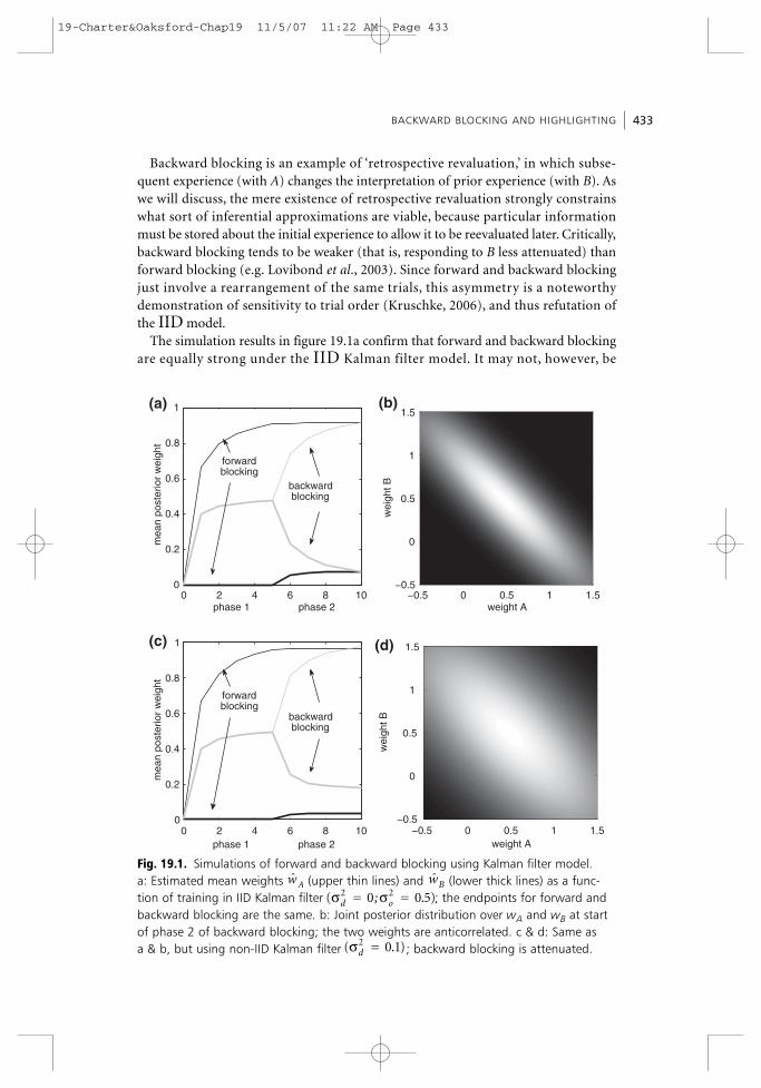
A subtler trial order dependence also arises in the form of a robust highlightingeffect (Figure 19.3a). This traces to three interlinked features of the model.


0 10 20 30 40

S −1

−0.5

0

0.5

R 1

mea

n po

ster

ior

pred

ictio

n

phase 1 phase 2

B

A

BC

C

(a)

0 10 20 30 400.2

0.4

0.6

0.8

1

1.2

1.4

1.6

post

erio

r un

cert

aint

y

phase 1 phase 2

A

B

C

(b)

0 10 20 30 40 S −1

−0.5

0

0.5

R 1

pred

ictio

n (p

oint

est

imat

e)

phase 1 phase 2

B

A

BC

C

(c)

0 10 20 30 400

0.5

1

estim

ated

mix

ing

prop

ortio

n

phase 1 phase 2

A

B

C

(d)

Fig. 19.3. Simulations of highlighting in approximate Bayesian reasoning. (a) Highlight-ing in Kalman filter with diagonalized assumed covariance . (b) Posterior uncertainty about each weight as a function of training; is more uncer-tain in first phase, highlighting it. (c) Highlighting in additive Gaussian mixture modelusing EM (η= 0.1; illustrated are the point estimates of the three individual weights and,for compound BC, the net outcome expectation weighted by mixing proportions). (d) Development of estimates of mixing proportions with training; C is highlighted.

wC

( )σ σd o= ; =2 20.1 0.5

ii This minimizes the KL-divergence from the full covariance Gaussian among the class of alldiagonal distributions.


First, much like attentional variables in associative accounts of highlighting(Kruschke, 2003), in the Kalman filter, the uncertainties about the weights (the diago-nal elements of the covariance matrix) control the rate of learning about thoseweights (Dayan and Long; Kakade and Dayan, 2002). More uncertain weights get alarger gain k and a bigger update from Equation 7; when stimuli are observed, theuncertainties about them (and subsequent learning rates) decline, whereas whenstimuli are unobserved, their uncertainties increase. This means (Figure 19.3b) thaton AC→S trials in the first block, C (which is rarely observed) learns more rapidlythan A (which is commonly observed). Conversely, A is likely to be paired with R thefirst few times it is seen, when its learning rate is highest. Second, the weights of pre-sented stimuli must interact additively to produce the outcome (Equation 2).A’s asso-ciation with R will therefore reduce B’s association with it (since the two weights mustadditively share the prediction on AB→R trials), whereas C’s association with S willbe correspondingly enhanced by additionally having to cancel out A’s opposing pre-diction of R. Finally, since the covariance is not represented, A is never retrospectivelyrevalued as a nonpredictor – its initial association with R instead persists indefinitelyas a primacy effect. There is a continuum of possible values , and thattogether add up to explain exactly the results of both trial types (specifically

and for any ); lacking revaluation, this model stickswith the first one it finds.

Note also that the venerable Rescorla–Wagner model results from one further sim-plification over this one: the assumption that the learning rates are simply constant (if perhaps stimulus-dependent), i.e. that the uncertainties are never updated. This ismotivated by the fact that, under special circumstances, for instance, if each stimulusis presented on every trial, the Kalman filter ultimately evolves to a fixed asymptoticlearning rate (the value at which information from each observation exactly balancesout diffusion in the prior). However, from the perspective of highlighting, this is asimplification too far, since without dynamic learning rates C’s learning about S is notboosted relative to A. Similar to the full Kalman filter, no highlighting effect is seen:the local base rates predominate. The lack of covariance information also prevents itfrom exhibiting backward blocking.

4.2 Maximum Likelihood and Expectation MaximizationSimilar phenomena can be seen, for similar reasons, in other approximation schemes.We exemplify this generality using a representative member of another class of inex-act but statistically grounded approaches, namely those that attempt to determine justa maximum likelihood point-estimate of the relevant variables (here the means )rather than a full posterior distribution over them. Often, these methods learn usingsome sort of hill climbing or gradient approach, and, of course, it is not possible toemploy Bayes’ theorem directly without representing some form of a distribution. Asfor assumed density filters (and for the Rescorla–Wagner model, which can also beinterpreted as a maximum-likelihood gradient climber), the failure to maintain anadequate posterior distribution curtails or abolishes retrospective revaluation.

Another example is a particular learning algorithm for the competitive mixture ofGaussians model of Equation 3. We develop this in some detail as it is the canonical

w

wAˆ ˆw = wC A− −1ˆ ˆw = wB A1 −

wCwBwA



example of a particularly relevant learning algorithm and is related to a number ofimportant behavioral models (Kruschke, 2001; Mackintosh, 1975), though it doeshave some empirical shortcomings related to its assumptions about cue combination(Dayan and Long, 1998). Recall that, according to this generative model, one stimulusout of those presented will be chosen and the outcome will then be determined solelybased on the chosen stimulus’ weight. Learning about the weight from the outcomethen depends on unobserved information: which stimulus was chosen. Expectation-maximization methods (Dempster et al., 1977; Griffiths and Yuille, this volume)address this problem by repeatedly alternating two steps: estimating the hidden infor-mation based on the current beliefs about the weights (‘E step’), then updating theweights assuming this estimate to be true (‘M step’). This process can be understoodto perform coordinate ascent on a particular error function, and is guaranteed toreduce (or at least not increase) the error at each step (Neal and Hinton, 1998).

An online form of EM is appropriate for learning in the generative model ofEquation 3. (Assume for simplicity that the weights do not change, i.e., that Equation 4obtains.) At each trial, the E step determines the probability that the outcome wasproduced by each stimulus (or the background stimulus 0), which involves a Bayesianinversion of the generative model:

qtj µ xtjπtj exp(–(rt – wtj)2/σ0)

Here, the background responsibility and the constant ofproportionality in qt arrange for appropriate normalization. The model then learns anew point estimate of the weights and the mixing proportions using what isknown as a partial M step, with the predictions associated with each stimulus chang-ing according to their own prediction error, but by an amount that depends on theresponsibilities accorded to each during the E step:

(9)

(10)

Here, η is a learning rate parameter, which, as for the Rescorla–Wagner rule, by beingfixed, can be seen as a severe form of approximation to the case of continual change inthe world.

4.2.1 SimulationsLike most other more or less local hill climbing methods, the fact that the M-step inthis algorithm is based on the previous, particular, parameter settings (through themedium of the E-step) implies that there are trial order effects akin to primacy. AsFigure 19.3c illustrates, these include highlighting, which arises here because theresponsibilities (and the estimated mixing variables that determine and are deter-mined by them) take on an attentional role similar to the uncertainties in the diago-nalized Kalman filter account. In particular, A and B share responsibility q (Figure 19.3d)for the preponderance of R in the first block. This reduces the extent to which learns about R (since the effective learning rate is ηqB), and the extent to which B

wB

ππ

ˆ ˆ ( ˆ ),π π η πt j tj tj tj tjx q+ = + −1

ˆ ˆ ( ˆ ),w w q r wt j tj tj t tj+ = + −1 η

πw

ˆ max( ˆ )πt t t= ,0 1 0− ⋅ππ x



contributes to the aggregate prediction during the BC probe (since B’s contribution tothe expectation is proportional to ). Meanwhile, by the second block of trials, themodel has learned that A has little responsibility ( is low), giving a comparativeboost to learning about during the now-frequent S trials. Less learning about due to its lower responsibility also means its association with R persists as a primacyeffect. These biases follow from the way the evolving beliefs about the stimuli participate in the approximate learning rule through the determination of responsi-bilities – recall that we derived the model using the IID assumption and that optimalinference is, therefore, trial order independent.

Note that unlike the diagonal Kalman filter example of Figure 19.3a, the highlight-ing effect here doesn’t arise until the second block of trials. This means that this EMmodel doesn’t explain the ‘inverse base rate effect,’ (Medin and Edelson, 1988) whichis the highlighting effect shown even using only the first block when R predominates.One reason for this, in turn, is the key competitive feature of this rule, that the predictions made by each stimulus do not interact additively in the generative rule(Equation 3). Because of this, while stimuli may share responsibility for the outcome,the net prediction doesn’t otherwise enter into the learning rule of Equation 9, whichstill seeks to make each stimulus account for the whole outcome on its own. In high-lighting, this means A’s association with R cannot directly boost C’s association with Sduring the first phase. The same feature also causes problems for this model (and itsassociative cousins) explaining other phenomena such as overshadowing andinhibitory conditioning, and ultimately favors alternatives to Equation 3 in whichcues cooperate to produce the net observation (Dayan and Long, 1998; Hinton, 1999;Jacobs et al., 1991a).

Despite this failure, the competitive model does exhibit forward blocking, albeitthrough a responsibility-sharing mechanism (Mackintosh, 1975) rather than aweight-sharing mechanism like Rescorla–Wagner (simulations not illustrated). Moreconcretely, stimulus A claims responsibility for R on AB→R trials, due to already pre-dicting it. This retards learning about B, as in blocking. However, given that it is basedonly on a point-estimate, it retains no covariance information, and so, likeRescorla–Wagner, cannot account for backward blocking.

4.3 SummaryWe have shown how two rather different sorts of inferential approximation schemes,in the context of two different generative models for conditioning, both disrupt retro-spective revaluation – abolishing backward blocking and producing a highlightingeffect. Exact Bayesian reasoning is characterized by simultaneously maintaining thecorrect likelihood for every possible hypothesis. This is what enables retrospectivelyrevisiting previously disfavored hypotheses when new data arrive, but it is also themain source of computational complexity in Bayesian reasoning and the target for simplification schemes. In short, primacy effects – the failure retrospectivelyto discount an initially favored hypothesis – are closely linked to inferential approximation.We have used extreme approximations to expose this point as clearly as possible.While the experiments discussed here both suggest that retrospective revaluation is

wAwC

πA

πB



attenuated, that effects like backward blocking exist at all rules out such extremeapproaches. In the following section, we consider gentler approximations.

5 Blended and Mixed ApproximationsSo far, neither the Bayesian nor the approximately Bayesian models actually exhibitthe combination of recency and primacy evident in backward blocking and highlight-ing. In fact, this is not hard to achieve, as there are a number of models that naturallylie between the extremes discussed in Sections 3 and 4. The cost is one additionalparameter. In this section, we provide two examples, based on different ideas associ-ated with approximating the Kalman filter.

5.1 Reduced-rank ApproximationsIn Section 4.1, we considered the simplest possible assumed density version of theKalman filter, in which the posterior fully factorized, having a diagonal covariancematrix (Figure 19.3a). This method fails to exhibit backwards blocking, since it can-not represent the necessary anticorrelation between the predictions of the two CSsthat arises during the first set of learning trials.

A less severe approximation to the posterior is to use a reduced-rank covariancematrix. We use one that attempts to stay close to the inverse covariance matrix, which(roughly speaking) characterizes certainty. An approximation of this sort allows thesubject to carry less information between trials (because of the reduction in rank),and can also enable simplification of the matrix calculations for the subsequentupdate to the Kalman filter (Treebushny and Madsen, 2005).

More precisely, we approximate the inverse posterior covariance after one trial,(St – κt xt St)

-1, by retaining only those n basis vectors from its singular value decom-position that have the highest singular values, thereby minimizing the Frobenius normof the difference. On the next trial we reconstruct the covariance as the pseudo-inverseof the rank-n matrix plus the uncertainty contributed by the intervening drift, .

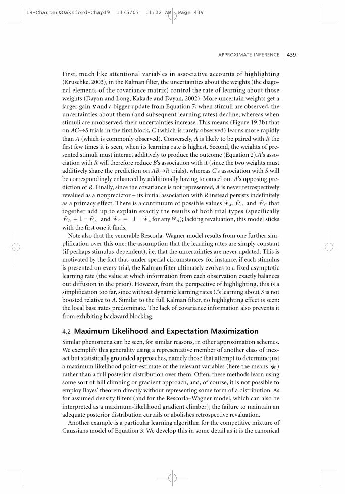
Figure 19.4a,b shows the consequence of using a rank-2 approximation (n = 2) tothe covariance matrix. This results in highlighting without further disrupting back-ward blocking, which, in any case, only requires a two-dimensional posterior. A gen-eral prediction of this sort of resource bottleneck approach is that the effects ofapproximation should become more pronounced – e.g. retrospective revaluationmore attenuated – for problems involving higher dimensional and more intricatelystructured posteriors.

5.2 Mixing FiltersA different possibility is to mix the exact and diagonally approximated Kalman filtersmore directly. Here the idea is that there may be mixing at the behavioral level of dis-tinct underlying psychological and/or neural processes, one corresponding to eachmodel. In some circumstances – for instance, when the diagonal elements of thecovariance matrix are anyway small – the additional accuracy to be gained by main-taining the full covariance matrix may not justify the additional energetic costs rela-tive to the particularly simple diagonal version. Such considerations suggest that the

σd2I



brain could adaptively trade off whether to employ approximation based on a sort ofmeta-rational cost-benefit analysis. (In this case, blending would appear in results viathe average over trials or subjects.) A slightly different version of this idea would sug-gest that subjects actually compute both forms simultaneously, but then reconcile theanswers, making an adaptive decision how much to trust each, much as in other casesof Bayesian evidence reconcilation (Daw et al., 2005). The ‘exact’ computation mightnot always be the most accurate, if in biological tissue the extra computations incuradditional computational noise; it might therefore be worthwhile to expend extraresources also computing a less noisy approximation.

Figure 19.2c,d shows simulations of a model which performs mixing by multiply-ing the off-diagonal elements of the covariance S by 0.7 at each step. This restricts theefficacy of retrospective revaluation without totally preventing it, allowing both back-ward blocking, which is curtailed relative to forward blocking, and highlighting.

6 Discussion

6.1 SummaryIn this chapter, we have focused on the intricacies of inference in Bayesian models ofconditioning. We used theory and simulations to show how particular classes of effects

DISCUSSION 443

0 10 20 30 40

S −1

−0.5

0

0.5

R 1

mea

n po

ster

ior

pred

ictio

n

phase 1 phase 2

B

A

BC

C

(a)

0 2 4 6 8 100

0.2

0.4

0.6

0.8

1

mea

n po

ster

ior

wei

ght

phase 1 phase 2

backwardblocking

forwardblocking

(b)

0 10 20 30 40

S −1

−0.5

0

0.5

R 1

mea

n po

ster

ior

pred

ictio

n

phase 1 phase 2

B

A

BC

C

(c)

0 2 4 6 8 100

0.2

0.4

0.6

0.8

1

mea

n po

ster

ior

wei

ght

phase 1 phase 2

backwardblocking

forwardblocking

(d)

Fig. 19.4. Simulations of two approximate Bayesian models exhibiting highlighting and backwards blocking. (a,b) Reduced-rank covariance Kalman filter

. (c,d) Blended full/diagonal covariance Kalman filter.(σ σd o= ; =2 20.1 0.1)

(σ σd o= ; = ;n =2 20.1 0.5 2)


in learning (e.g. backward blocking) can arise from optimal inference in the light of asimple generative model of a task, and others (e.g. highlighting) from more or lessextreme, but still recognizable approximations to optimal inference. This work on sen-sitivity to trial order is clearly only in its infancy, and the data to decide between andrefine the various different models are rather sparse. However, just as we try to differ-entiate subjects’ assumptions in exact Bayesian modeling, we hope in the future toadjudicate more definitively between different approximation methods by identifyingtasks that better expose their fingerprints. Here, we have focused on trial order, butmany similar issues arise in other areas of conditioning, such as stimulus competition.

6.2 Locally Bayesian LearningOne spur to study trial order was the recent article by Kruschke (2006). He pointedout the apparent contradiction between the recency in backward blocking and theprimacy in highlighting, and noted the implications of the IID assumption for bothphenomena. Kruschke framed these findings by contrasting classic associative learn-ing models (which explain highlighting via ideas about stimulus attention) with aparticular IID Bayesian model (which explains retrospective revaluation). Rather thanaddressing the IID assumption (which, of course, Bayesian models need not make),he proposed a ‘locally Bayesian’ model blending features of both of these approaches.This model consists of interconnected modules that are Bayesian-inspired in thateach updates a local belief distribution using Bayes’ rule, but heuristic in that the‘observations’ to which Bayes’ rule is applied are not observed data but instead syn-thetic quantities constructed using an ad-hoc message-passing scheme. Although theindividual modules treat their synthetic data as IID, trial ordering effects emerge fromtheir interactions. The theoretical status of the heuristic, for instance as a particularform of approximation to a well-found statistical procedure, is left unclear.

We have attempted to address the issues central to highlighting and backwardsblocking in unambiguously Bayesian terms. We develop a similar contrast betweenexact and approximate approaches, but rather than seeing statistical and associativelearning as contradictory and requiring reconciliation, we have stressed their connec-tion under a broader Bayesian umbrella. The approximate Kalman filters discussed inSection 5 retain a precise flavor of the optimal solutions, while offering parameterizedroutes to account for the qualitative characteristics of both backwards blocking andhighlighting.

It is also possible to extend this broader Bayesian analysis to the mixture model ofSection 4.2, and hence nearer to Kruschke’s (2006) locally Bayesian scheme. The mix-ture model fails to exhibit retrospective revaluation since it propagates only a point,maximum likelihood, estimate of the posterior distribution over the weights. Thiscould be rectified by adopting a so-called ensemble learning approach (Hinton andvan Camp, 1993; Waterhouse et al., 1996), in which a full (approximate) distributionover the learned parameters is maintained and propagated, rather than just a pointestimate. In ensemble learning, this distribution is improved by iterative ascent (anal-ogous to E and M steps) rather than direct application of Bayes’ rule.

One online version of such a rule could take the form of inferring the unobservedresponsibilities, and then conditioning on them as though they were observed data



(see also the mixture update of Dearden et al. 1998). Since it conducts inference usingsynthetic in place of observed quantities, this rule would have the flavor of Kruschke’slocally Bayesian scheme, and indeed would be a route to find statistically justifiableprinciples for his model. However, this line of reasoning suggests one key modifica-tion to his model, that the unobserved quantities should be estimated optimally fromthe statistical model using an E step, obviating the need for a target propagationscheme.

6.3 Bayes, Damn Bayes, and ApproximationsAt its core, the Bayesian program in psychology is about understanding subjects’behavior in terms of principles of rational inference. This approach extends directlybeyond ideal computation in the relatively small set of tractably computable modelsinto approximate reasoning in richer models. Of course, we cannot interrogate evolution to find out whether some observable facet of conditioning arises as exactinference in a model that is a sophisticated adaptation to a characteristic of the learn-ing environment that we have not been clever enough to figure out, or as an inevitableapproximation to inference in what is likely to be a simpler model. Nevertheless,admitting well found approximations does not infinitely enlarge the family of candi-date models, and Occam’s razor may continue to guide.

Waldmann et al. (2007; this volume) pose another version of our dilemma. Theyagree with Churchland (1986) that the top-down spirit of Marrian modeling is alwaysviolated in practice, with practitioners taking peeks at algorithmic (psychological)and even implementational (neural) results before building their abstract, computa-tional accounts. However, unlike the approach that we have tried to follow, their solu-tion is to posit the notion of a minimal rational model that more explicitly elevatesalgorithmic issues into the computational level.

We see two critical dangers in the Waldmann ‘minimal rationality’ programme, oneassociated with each of the two words. One danger Marr himself might have worriedabout, namely the fact that minimality is in the eye of the beholder (or at least theinstruction set), and that our lack of a justifiable account of the costs of neural pro-cessing makes any notion of minimality risk vacuity. The second danger is that byblending normative considerations with incommensurate pragmatic ones, minimalrationality risks being a contradiction in terms. We agree with Waldmann and col-leagues’ criticism that rational theorists have sometimes been a bit glib relating theo-ries of competence to performance, but we see the solution in taking this distinctionmore seriously rather than making it murky. Since computational and algorithmiclevels involve fundamentally different questions (e.g. why versus how), we suggestpreserving the innocence of the computational account, and focusing on approxima-tions at the algorithmic level.

Finally, as we saw in Section 5.2, one important facet of approximate methods isthat it is frequently appropriate to maintain multiple different approximations, eachof which is appropriate in particular circumstances, and to switch between or blendtheir outputs. To the extent that different approximations lead to different behavior, itwill be possible to diagnose and understand them and the tradeoffs that they (locally)optimize. Our understanding of the blending and switching process is less advanced.

DISCUSSION 445


In the present setting, the idea goes back at least to Konorski (1967) that Pavlovianlearning can employ both a stimulus-stimulus pathway (which is more cognitive inthis respect and echoes our full Kalman filter’s representation of interstimulus covari-ance) and a simpler stimulus-reward one (perhaps related to our diagonalizedKalman filter); such processes also appear to be neurally distinguishable (Balleine andKillcross, 2006). In fact, there is evidence for similar behavioral dissociations comingfrom attempts to demonstrate retrospective revaluation in rats (Miller and Matute,1996). When training is conducted directly in terms of stimulus-reinforcer pairings,no retrospective revaluation is generally seen (as with our diagonalized covarianceKalman filter), but revaluation does succeed in the more obviously cognitive case inwhich the paradigms are conducted entirely in terms of pairings between affectivelyneutral stimuli, one of which (standing in for the reinforcer) is finally associated withreinforcement before the test phase.

Parallel to this in the context of instrumental conditioning is an analogous divisionbetween an elaborate, cognitive, (and likely computationally noisy) ‘goal-directed’pathway, and a simpler (but statistically inefficient) ‘habitual’ one (Dickinson andBalleine, 2002). In this setting, the idea of normatively trading off approximate value-inference approaches characteristic of the systems has been formalized in terms oftheir respective uncertainties, and explains a wealth of data about what circumstancesfavor the dominance of goal-directed or habitual processes (Daw et al., 2005). Itwould be interesting to explore similar estimates of uncertainty in the mixed Kalmanfilters and thereby gain normative traction on the mixing.

ReferencesBalleine, B. W., & Killcross, S. (2006). Parallel incentive processing: An integrated view of amyg-

dala function. Trends in Neurosciences, 29, 272–279

Chomsky, N. (1965) Aspects of the Theory of Syntax. MIT Press.

Churchland, P. S. (1986). Neurophilosophy: Toward a unified science of the mind-brain.Cambridge, MA: MIT Press

Courville, A. C., Daw, N. D., Gordon, G. J., & D. S. Touretzky (2003). Model uncertainty in classical conditioning. In Advances in Neural Information Processing Systems (Vol. 16).Cambridge, MA: MIT Press.

Courville, A. C., Daw, N. D., & Touretzky, D. S. (2004). Similarity and discrimination in classical conditioning: A latent variable account. In Advances in Neural InformationProcessing Systems (Vol. 17). Cambridge, MA: MIT Press.

Courville, A. C., Daw, N. D., & Touretzky, D. S. (2006). Bayesian theories of conditioning in achanging world. Trends in Cognitive Sciences, 10, 294–300.

Daw, N. D., Niv, Y., & Dayan, P. (2005). Uncertainty-based competition between prefrontal anddorsolateral striatal systems for behavioral control. Nature Neuroscience, 8, 1704–1711.

Daw, N. D., O’Doherty, J. P., Seymour, B., Dayan, P., & Dolan, R. J. (2006). Cortical substratesfor exploratory decisions in humans. Nature, 441, 876–879.

Dayan, P., & Long, T. (1998). Statistical models of conditioning. Advances in Neural InformationProcessing Systems, 10, 117–123.

Dayan, P., Kakade, S., & Montague P. R. (2000). Learning and selective attention. NatureNeuroscience, 3, 1218–1223.



Dearden, R., Friedman N., & Russell S. J. (1998). Bayesian Q-learning. In Proceedings of the 15th National Conference on Artificial Intelligence (AAAI), PP. 761–768.

Dempster A. P., Laird N. M., & Rubin D. B. (1977). Maximum likelihood from incomplete datavia the EM algorithm. Journal of the Royal Statistical Society B, 39, 1–38.

Dickinson, A., & Balleine, B. (2002). The role of learning in motivation. In C. R. Gallistel (Ed.),Stevens’ handbook of experimental psychology Vol. 3: Learning, Motivation and Emotion(3rd ed., pp. 497–533). New York: Wiley.

Doucet, A., Godsill, S., & Andrieu, C. (2000). On sequential Monte Carlo sampling methods forBayesian filtering. Statistics and Computing, 10, 197–208.

Griffiths, T. L., & Yuille, A. (2007). Technical introduction: A primer on probabilistic inference.2007. (this volume).

Hinton, G. (1999). Products of experts. In Proceedings of the Ninth International Conference onArtificial Neural Networks (ICANN99), pp. 1–6.

Hinton, G., & van Camp, D. (1993). Keeping neural networks simple by minimizing thedescription length of the weights. In Proceedings of the Sixth Annual ACM Conference onComputational Learning Theory, pp. 5–13.

Jacobs, R. A., Jordan, M. I., & Barto, A. G. (1991a). Task decomposition through competition ina modular connectionist architecture: The what and where vision tasks. Cognitive Science,15, 219–250.

Jacobs, R. A., Jordan, M. I., Nowlan, S. J., & Hinton, G. E. (1991b). Adaptive mixtures of localexperts. Neural Computation, 3, 79–87.

Jordan, M. I., Ghahramani, Z., Jaakkola, T. S., & Saul, L. K. (1999). An introduction to varia-tional methods for graphical models. Machine Learning, 37, 183–233.

Kakade, S., & Dayan, P. (2001). Explaining away in weight space. In Advances in NeuralInformation Processing Systems (Vol. 13). Cambridge, MA: MIT Press.

Kakade, S., & Dayan, P. (2002). Acquisition and extinction in autoshaping. Psychological Review,109, 533–544.

Kalman, R. E. (1960). A new approach to linear filtering and prediction problems. Transactionsof the ASME–Journal of Basic Engineering, 82, 35–45.

Kamin, L. J. (1969). Predictability, surprise, attention, and conditioning. In B. A. Campbell & R. M. Church (Eds.), Punishment and aversive behavior (pp. 242–259). New York:Appleton-Century-Crofts.

Konorski, J. (1967) Integrative activity of the brain. University of Chicago Press: Chicago.

Kruschke, J. K. (2001). Toward a unified model of attention in associative learning. Journal ofMathematical Psychology, 45, 812–863.

Kruschke, J. K. (2006). Locally Bayesian learning with applications to retrospective revaluationand highlighting. Psychological Review, 113, 677–699.

Kruschke, J. K. (2003). Attention in learning. Current Directions in Psychological Science,5, 171–175.

Lovibond, P. F., Been, S.-L., Mitchell, C. J., Bouton, M. E., & Frohardt, R. (2003). Forward andbackward blocking of causal judgment is enhanced by additivity of effect magnitude.Memory and Cognition, 31, 133–142.

Mackintosh, N. J. (1975). A theory of attention: Variations in the associability of stimuli withreinforcement. Psychological Review, 82, 532–552.

Marr, D. (1982). Vision: A computational approach. San Francisco, CA: Freeman and Co.

Medin, D. L., & Bettger, J. G. (1991). Sensitivity to changes in base-rate information. AmericanJournal of Psychology, 40, 175–188.

REFERENCES 447


Medin, D. L., & Edelson, S. M. (1988). Problem structure and the use of base-rate informationfrom experience. Journal of Experimental Psychology: General, 117, 68–85.

Miller, R. R., & Matute, H. (1996). Biological significance in forward and backward blocking:Resolution of a discrepancy between animal conditioning and human causal judgment.Journal of Experimental Psychology: General, 125, 370–386.

Minka, T. (2001). A family of algorithms for approximate Bayesian inference. PhD thesis,Massachusetts Institute of Technology.

Neal, R. M., & Hinton, G. E. (1998). A view of the EM algorithm that justifies incremental,sparse and other variants. In M. I. Jordan (Ed.), Learning in graphical models (pp. 355–368).Kluwer Academic Publishers.

Rescorla, R. A., & Wagner, A. R. (1972). A theory of Pavlovian conditioning: The effectivenessof reinforcement and non-reinforcement. In A. H. Black & W. F. Prokasy (Eds.), Classicalconditioning, 2: Current research and theory (pp. 64–69). New York: Appleton Century-Crofts.

Shanks, D. R. (1985). Forward and backward blocking in human contingency judgement.Quarterly Journal of Experimental Psychology, 37B, 1–21.

Simon, H. (1957). A behavioral model of rational choice. In Models of man, social and rational:Mathematical essays on rational human behavior in a social setting. Wiley, New York.

Treebushny, D., & Madsen, H. (2005). On the construction of a reduced rank square-rootKalman filter for efficient uncertainty propagation. Future Generation Computer Systems,21, 1047–1055.

Waldmann, M. R., Cheng, P. W., Hagmayer, Y., & Blaisdell, A. P. (2007). Causal learning in ratsand humans: A minimal rational model (this volume).

Wasserman, E. A., & Berglan, L. R. (1998). Backward blocking and recovery from overshadow-ing in human causal judgment: The role of within-compound associations. QuarterlyJournal of Experimental Psychology, 51B, 121–138.

Waterhouse, S., MacKay, D., & Robinson, T. (1996). Bayesian methods for mixtures of experts.Advances in Neural Information Processing Systems, 8, 351–357.

Yu, A. J., & Dayan, P. (2003). Expected and unexpected uncertainty: ACh and NE in the neocortex. In Advances in Neural Information Processing Systems (Vol. 15). Cambridge, MA:MIT Press.

Yu, A. J., & Dayan, P. (2005). Uncertainty, neuromodulation, and attention. Neuron,46, 681– 692.



Documents

Semi-rational Models of Conditioning: The Case of Trial …dayan/papers/dawcourvday08.pdf · Semi-rational Models of Conditioning: The Case ... distinction between performance and