Embed Size (px)
Citation preview
Semiparametric Quantile and Expectile Regression
Thomas Kneib
Department of MathematicsCarl von Ossietzky University Oldenburg
Piraeus, 21.8.2010
Thomas Kneib Childhood Malnutrition in Developing and Transition Countries
Childhood Malnutrition in Developing and Transition Countries
• Malnutrition and childhood malnutrition in particular are among the main publichealth problems in developing and transition countries.
• Halfing the proportion of malnourished people in developing countries until 2015 isone of the United Nations Millennium goals.
• Statistical analyses can help in the development and evaluation of interventions.
• We use data from the 1998/99 India Demographic and Health Survey(http://www.measuredhs.com).
• Nationally representative cross-sectional study on fertility, family planning, maternaland child health, as well as child survival, HIV/AIDS, and nutrition.
• Information on 24.316 children is available (after excluding observations with missinginformation).
Semiparametric Quantile and Expectile Regression 1
Thomas Kneib Childhood Malnutrition in Developing and Transition Countries
• Childhood malnutrition is assessed by a Z-score formed from an appropriate anthro-pometric measure AI relative to a reference population:
Zi =AIi − µ
σ
where µ and σ refer to median and standard deviation in the reference population.
• Chronic undernutrition (stunting) is measured by insufficient height for age.
• Children are classified as stunted based on lower quantiles from reference charts suchas the WHO Child Growth Standards.
Semiparametric Quantile and Expectile Regression 2
Thomas Kneib Childhood Malnutrition in Developing and Transition Countries
• Possible determinants of childhood malnutrition:
Child-specific factors: age, gender, duration of breastfeeding, . . .
Maternal factors: age, body mass index, years of education,employment status, . . .
Household factors: place of residence, electricity, radio, tv, . . .
(21 covariates in total).
• In addition, we have information on the district a child lives in
⇒ Spatial alignment of the data.
Semiparametric Quantile and Expectile Regression 3
Thomas Kneib Childhood Malnutrition in Developing and Transition Countries
• Regression models aim at quantifying the impact of covariates on undernutritionwhere the Z-score forms the response.
• Most common approach: Direct regression of the Z-score on covariates
Z = x′β + ε, ε ∼ N(0, σ2).
• Difficulties:
– All effects are assumed to be linear while effects of continuous covariates may besuspected to be nonlinear.
– The model does not allow for spatial effects.
– The direct regression model explains the expectation of Z, i.e. it focusses on theaverage nutritional status.
– Restrictive assumptions on the error terms ε.
⇒ Semiparametric quantile and expectile regression models.
Semiparametric Quantile and Expectile Regression 4
Thomas Kneib Quantile and Expectile Regression
Quantile and Expectile Regression
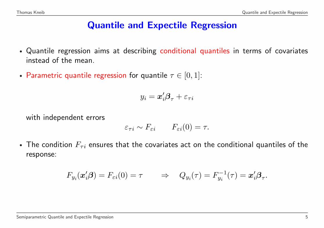
• Quantile regression aims at describing conditional quantiles in terms of covariatesinstead of the mean.
• Parametric quantile regression for quantile τ ∈ [0, 1]:
yi = x′iβτ + ετi
with independent errorsετi ∼ Fεi Fεi(0) = τ.
• The condition Fτi ensures that the covariates act on the conditional quantiles of theresponse:
Fyi(x′iβ) = Fεi(0) = τ ⇒ Qyi
(τ) = F−1yi
(τ) = x′iβτ .
Semiparametric Quantile and Expectile Regression 5
Thomas Kneib Quantile and Expectile Regression
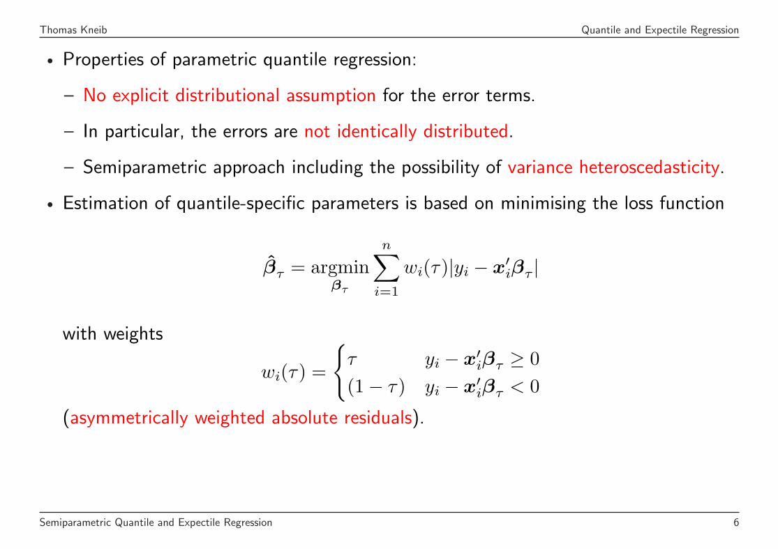
• Properties of parametric quantile regression:
– No explicit distributional assumption for the error terms.
– In particular, the errors are not identically distributed.
– Semiparametric approach including the possibility of variance heteroscedasticity.
• Estimation of quantile-specific parameters is based on minimising the loss function
βτ = argminβτ
n∑
i=1
wi(τ)|yi − x′iβτ |
with weights
wi(τ) =
{τ yi − x′iβτ ≥ 0(1− τ) yi − x′iβτ < 0
(asymmetrically weighted absolute residuals).
Semiparametric Quantile and Expectile Regression 6
Thomas Kneib Quantile and Expectile Regression
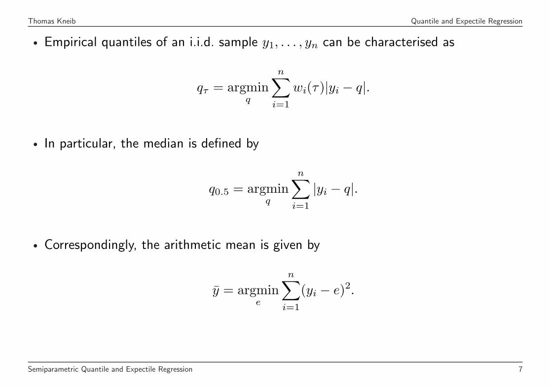
• Empirical quantiles of an i.i.d. sample y1, . . . , yn can be characterised as
qτ = argminq
n∑
i=1
wi(τ)|yi − q|.
• In particular, the median is defined by
q0.5 = argminq
n∑
i=1
|yi − q|.
• Correspondingly, the arithmetic mean is given by
y = argmine
n∑
i=1
(yi − e)2.
Semiparametric Quantile and Expectile Regression 7
Thomas Kneib Quantile and Expectile Regression
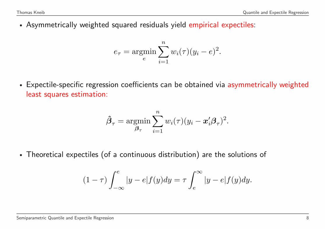
• Asymmetrically weighted squared residuals yield empirical expectiles:
eτ = argmine
n∑
i=1
wi(τ)(yi − e)2.
• Expectile-specific regression coefficients can be obtained via asymmetrically weightedleast squares estimation:
βτ = argminβτ
n∑
i=1
wi(τ)(yi − x′iβτ)2.
• Theoretical expectiles (of a continuous distribution) are the solutions of
(1− τ)∫ e
−∞|y − e|f(y)dy = τ
∫ ∞
e
|y − e|f(y)dy.
Semiparametric Quantile and Expectile Regression 8
Thomas Kneib Semiparametric Regression
Semiparametric Regression
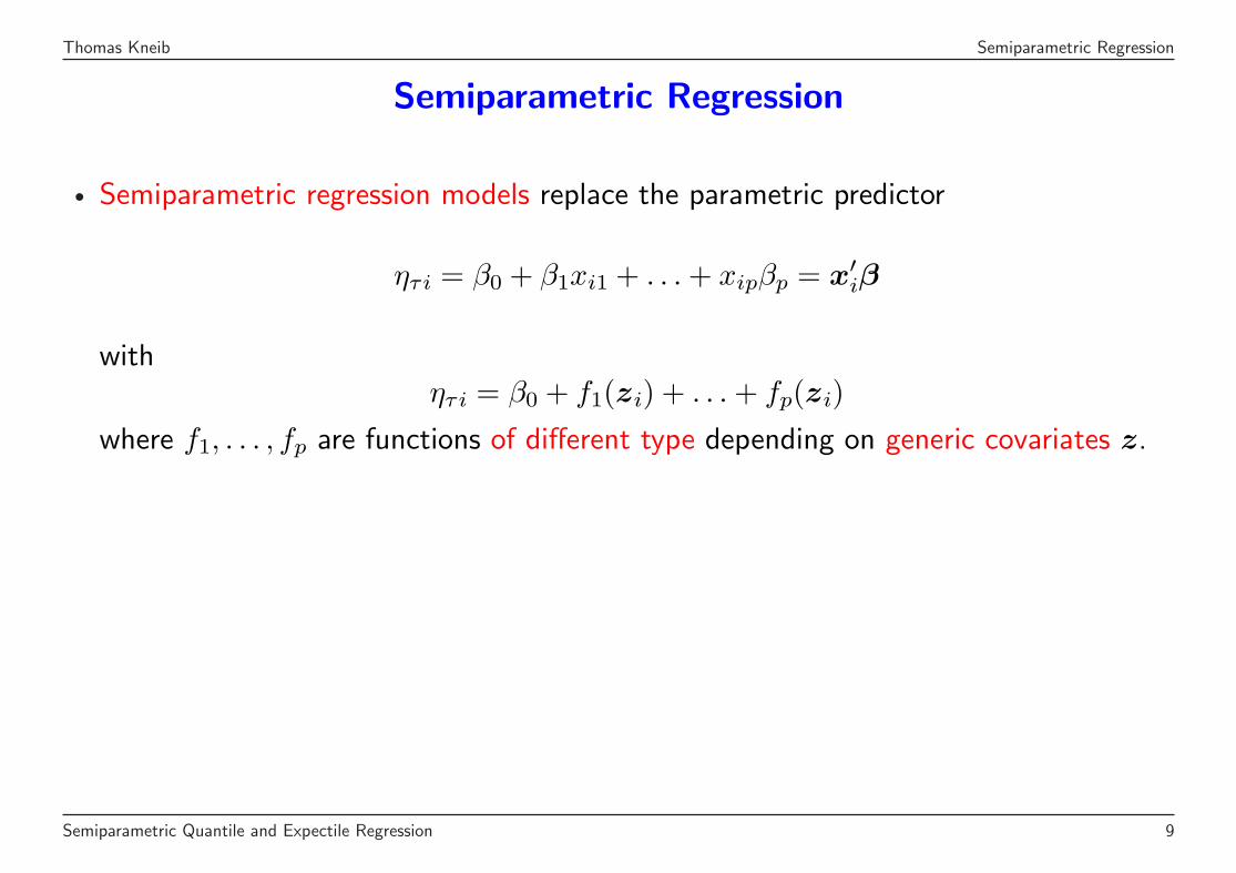
• Semiparametric regression models replace the parametric predictor
ητi = β0 + β1xi1 + . . . + xipβp = x′iβ
withητi = β0 + f1(zi) + . . . + fp(zi)
where f1, . . . , fp are functions of different type depending on generic covariates z.
Semiparametric Quantile and Expectile Regression 9
Thomas Kneib Semiparametric Regression
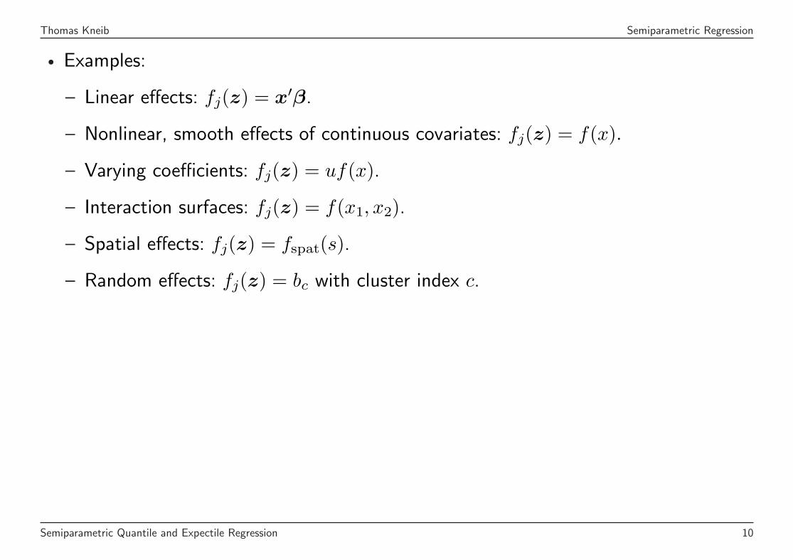
• Examples:
– Linear effects: fj(z) = x′β.
– Nonlinear, smooth effects of continuous covariates: fj(z) = f(x).
– Varying coefficients: fj(z) = uf(x).
– Interaction surfaces: fj(z) = f(x1, x2).
– Spatial effects: fj(z) = fspat(s).
– Random effects: fj(z) = bc with cluster index c.
Semiparametric Quantile and Expectile Regression 10

Thomas Kneib Semiparametric Regression
• Generic model description based on
– a design matrix Zj, such that the vector of function evaluations f j = (fj(z1),. . . , fj(zn))′ can be written as
f j = Zjγj.
– a quadratic penalty term
pen(fj) = pen(γj) = γ′jKjγj
which operationalises smoothness properties of fj.
• From a Bayesian perspective, the penalty term corresponds to a multivariate Gaussianprior
p(γj) ∝ exp
(− 1
2δ2j
γ′jKjγj
).
Semiparametric Quantile and Expectile Regression 11
Thomas Kneib Semiparametric Regression
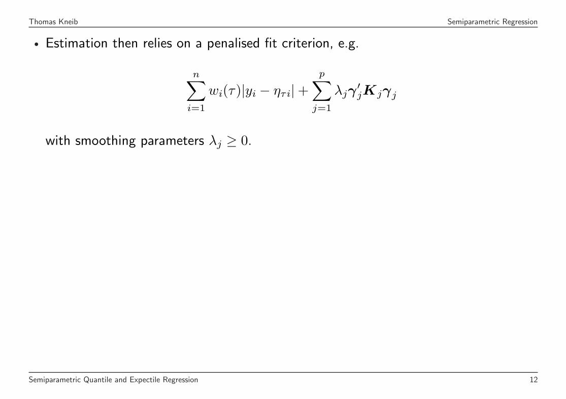
• Estimation then relies on a penalised fit criterion, e.g.
n∑
i=1
wi(τ)|yi − ητi|+p∑
j=1
λjγ′jKjγj
with smoothing parameters λj ≥ 0.
Semiparametric Quantile and Expectile Regression 12
Thomas Kneib Semiparametric Regression
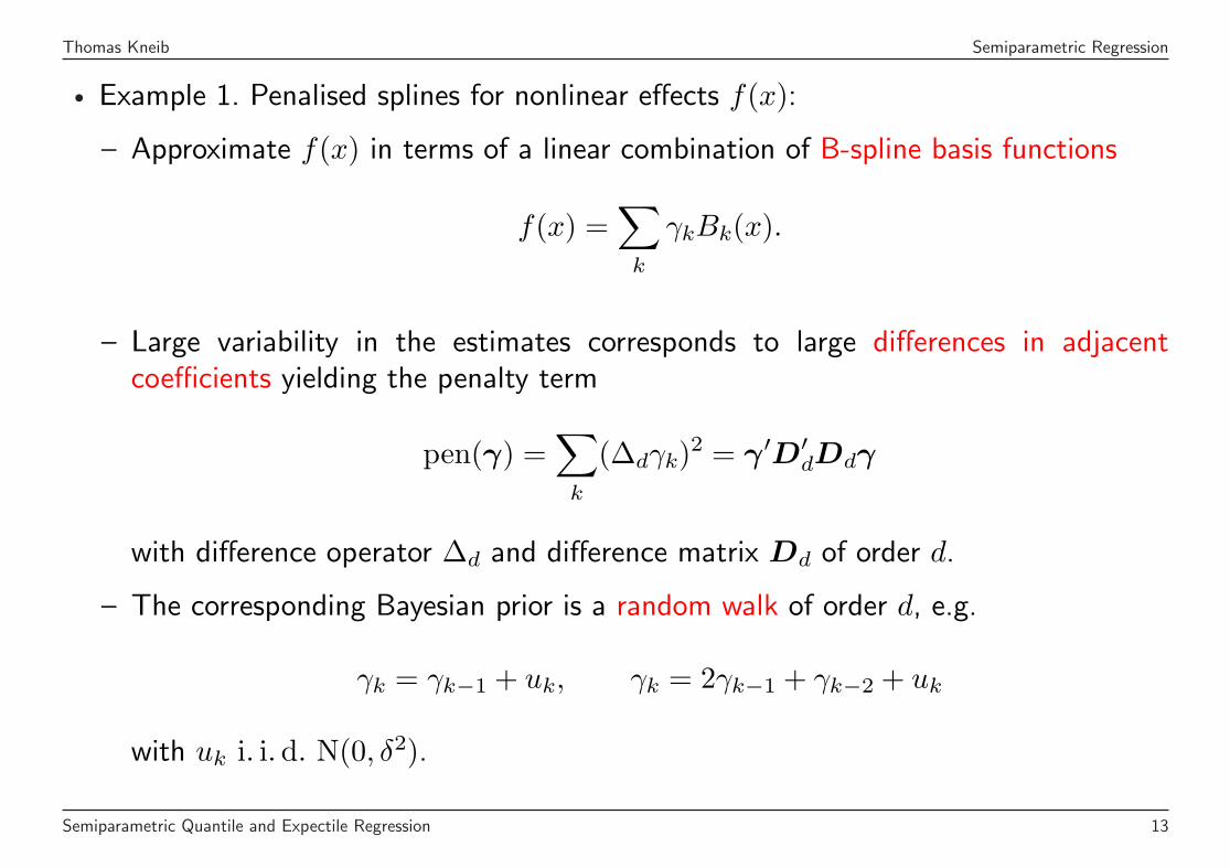
• Example 1. Penalised splines for nonlinear effects f(x):
– Approximate f(x) in terms of a linear combination of B-spline basis functions
f(x) =∑
k
γkBk(x).
– Large variability in the estimates corresponds to large differences in adjacentcoefficients yielding the penalty term
pen(γ) =∑
k
(∆dγk)2 = γ′D′dDdγ
with difference operator ∆d and difference matrix Dd of order d.
– The corresponding Bayesian prior is a random walk of order d, e.g.
γk = γk−1 + uk, γk = 2γk−1 + γk−2 + uk
with uk i. i. d. N(0, δ2).
Semiparametric Quantile and Expectile Regression 13

Thomas Kneib Semiparametric Regression
• Example 2. Markov random fields for the estimation of spatial effects based onregional data:
– Estimate a separate regression coefficient γs for each region, i.e. f = Zγ with
Z[i, s] =
{1 observation i belongs to region s
0 otherwise
– Penalty term based on differences of neighboring regions:
pen(γ) =∑
s
∑
r∈N(s)
(γs − γr)2 = γ′Kγ
where N(s) is the set of neighbors of region s and K is an adjacency matrix.
– An equivalent Bayesian prior structure is obtained based on Gaussian Markovrandom fields.
Semiparametric Quantile and Expectile Regression 14
Thomas Kneib Markov Chain Monte Carlo Simulations
Markov Chain Monte Carlo Simulations
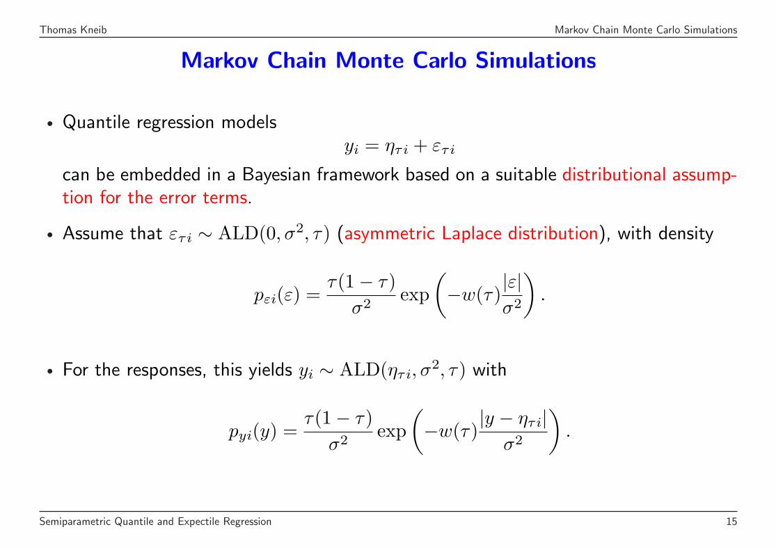
• Quantile regression modelsyi = ητi + ετi
can be embedded in a Bayesian framework based on a suitable distributional assump-tion for the error terms.
• Assume that ετi ∼ ALD(0, σ2, τ) (asymmetric Laplace distribution), with density
pεi(ε) =τ(1− τ)
σ2exp
(−w(τ)
|ε|σ2
).
• For the responses, this yields yi ∼ ALD(ητi, σ2, τ) with
pyi(y) =τ(1− τ)
σ2exp
(−w(τ)
|y − ητi|σ2
).
Semiparametric Quantile and Expectile Regression 15
Thomas Kneib Markov Chain Monte Carlo Simulations
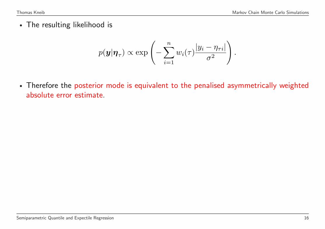
• The resulting likelihood is
p(y|ητ) ∝ exp
(−
n∑
i=1
wi(τ)|yi − ητi|
σ2
).
• Therefore the posterior mode is equivalent to the penalised asymmetrically weightedabsolute error estimate.
Semiparametric Quantile and Expectile Regression 16
Thomas Kneib Markov Chain Monte Carlo Simulations
• More precisely: The resulting point estimates coincide but the statistical estimateshave different properties.
• In particular, Bayesian quantile regression additionally assumes that
– the errors are identically distributed.
– the errors follow an asymmetric Laplace distribution.
• Consequences:
– The model is no longer semiparametric (with respect to the error distribution).
– The posterior is usually misspecified, such that measures of uncertainty should beinterpreted with care.
Semiparametric Quantile and Expectile Regression 17
Thomas Kneib Markov Chain Monte Carlo Simulations
• However, the posterior mean is easily obtained based on Markov chain Monte Carlosimulation techniques (even for very complex predictor structures)
• A Gibbs sampler can be constructed based on a location scale mixture of normalsrepresentation of the asymmetric Laplace distribution.
• Results in the imputation of additional unknowns but yields simple Gibbs updates.
Semiparametric Quantile and Expectile Regression 18
Thomas Kneib Markov Chain Monte Carlo Simulations
• Selected results for the malnutrition example:
– Estimates for the 5% quantile and the median.
– Note: Effects are centered and therefore the natural ordering of the 5% quantileand the median is not visible.
Semiparametric Quantile and Expectile Regression 19
Thomas Kneib Markov Chain Monte Carlo Simulations
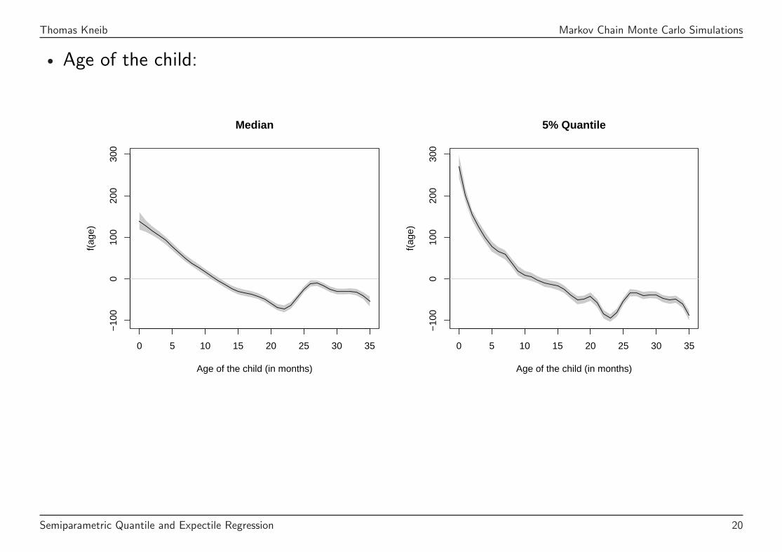
• Age of the child:
0 5 10 15 20 25 30 35
−10
00
100
200
300
Median
Age of the child (in months)
f(ag
e)
0 5 10 15 20 25 30 35
−10
00
100
200
300
5% Quantile
Age of the child (in months)
f(ag
e)
Semiparametric Quantile and Expectile Regression 20
Thomas Kneib Markov Chain Monte Carlo Simulations
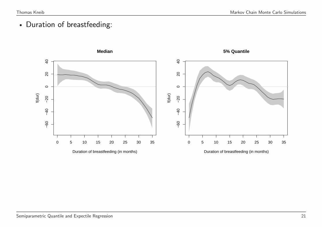
• Duration of breastfeeding:
0 5 10 15 20 25 30 35
−60
−40
−20
020
40Median
Duration of breastfeeding (in months)
f(du
r)
0 5 10 15 20 25 30 35
−60
−40
−20
020
40
5% Quantile
Duration of breastfeeding (in months)
f(du
r)
Semiparametric Quantile and Expectile Regression 21
Thomas Kneib Markov Chain Monte Carlo Simulations
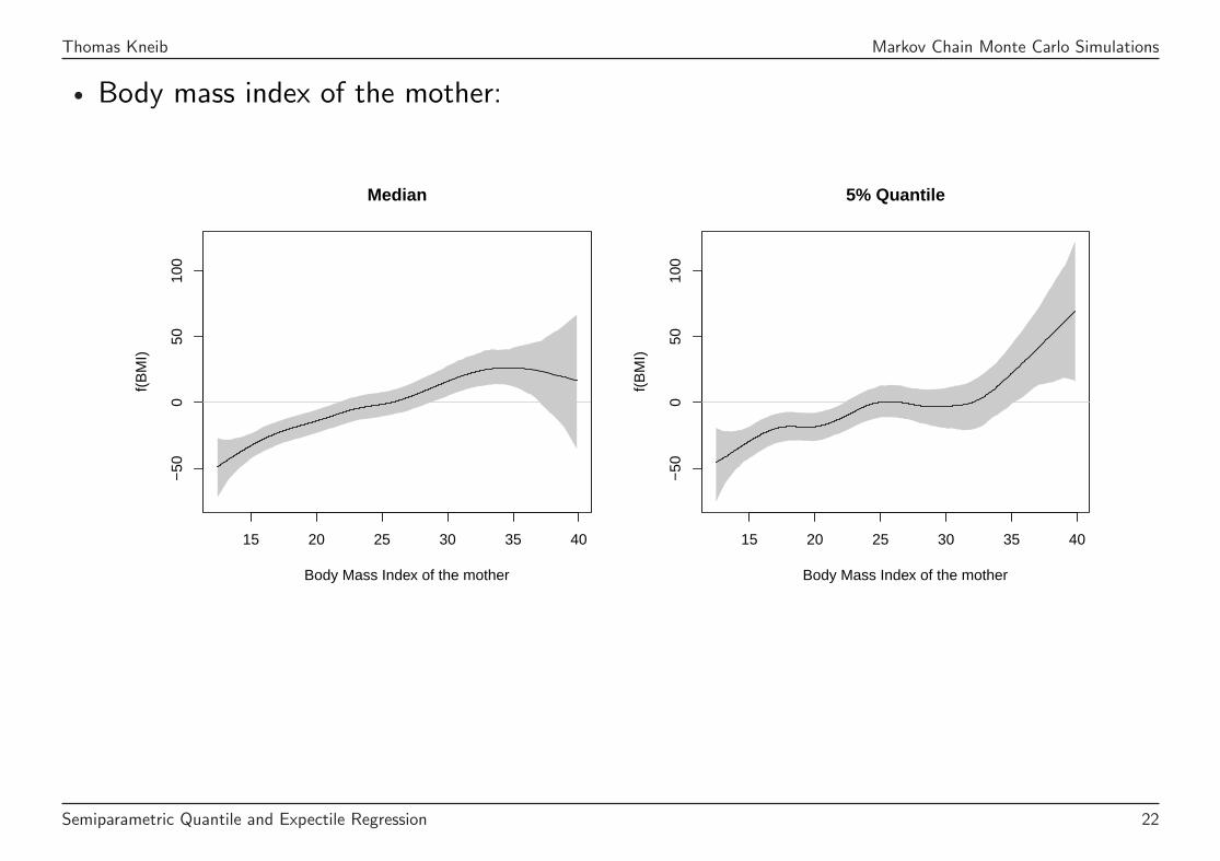
• Body mass index of the mother:
15 20 25 30 35 40
−50
050
100
Median
Body Mass Index of the mother
f(B
MI)
15 20 25 30 35 40
−50
050
100
5% Quantile
Body Mass Index of the mother
f(B
MI)
Semiparametric Quantile and Expectile Regression 22
Thomas Kneib Markov Chain Monte Carlo Simulations
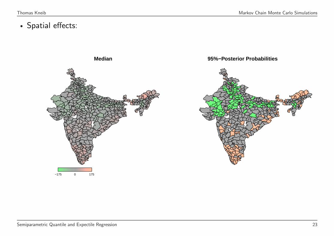
• Spatial effects:
Median
−175 1750
95%−Posterior Probabilities
Semiparametric Quantile and Expectile Regression 23
Thomas Kneib Markov Chain Monte Carlo Simulations
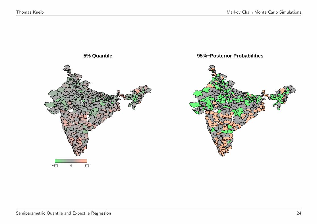
• Spatial effects:
5% Quantile
−175 1750
95%−Posterior Probabilities
Semiparametric Quantile and Expectile Regression 24

Thomas Kneib Asymmetrically Weighted Least Squares
Asymmetrically Weighted Least Squares
• Expectile-specific parameters are easier to obtain since the criterion
n∑
i=1
wi(τ)(yi − ητi)2 +p∑
j=1
λjγ′τjKjγτj
is differentiable with respect to the regression coefficients.
• Iteratively weighted penalised least squares estimation:
γτj = (Z ′jW (τ)Zj + λjKj)−1Z ′
jW (τ)(y − ητ + Zjγj).
• Smoothing parameters can be estimated based on a mixed model representationsimilar as in mean regression.
Semiparametric Quantile and Expectile Regression 25
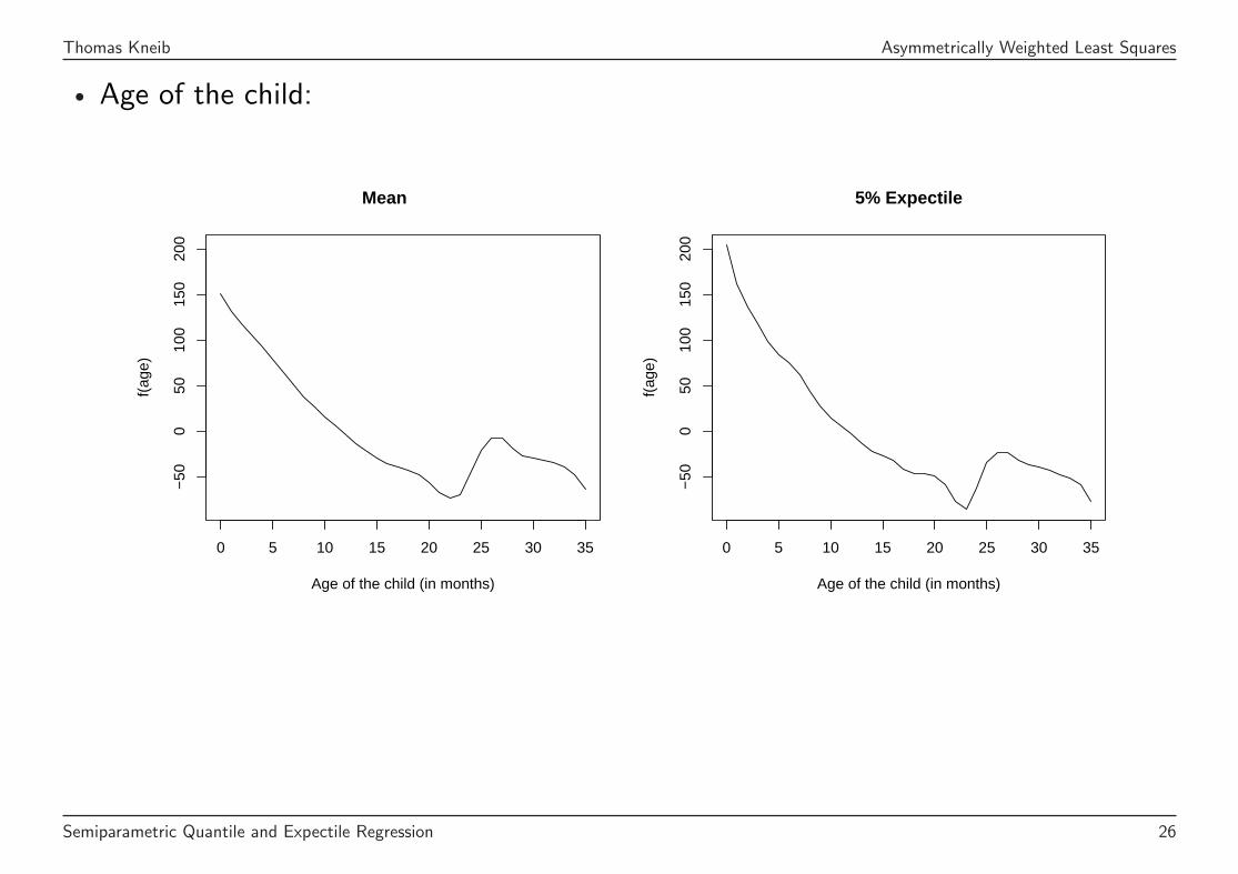
Thomas Kneib Asymmetrically Weighted Least Squares
• Age of the child:
0 5 10 15 20 25 30 35
−50
050
100
150
200
Mean
Age of the child (in months)
f(ag
e)
0 5 10 15 20 25 30 35
−50
050
100
150
200
5% Expectile
Age of the child (in months)
f(ag
e)
Semiparametric Quantile and Expectile Regression 26
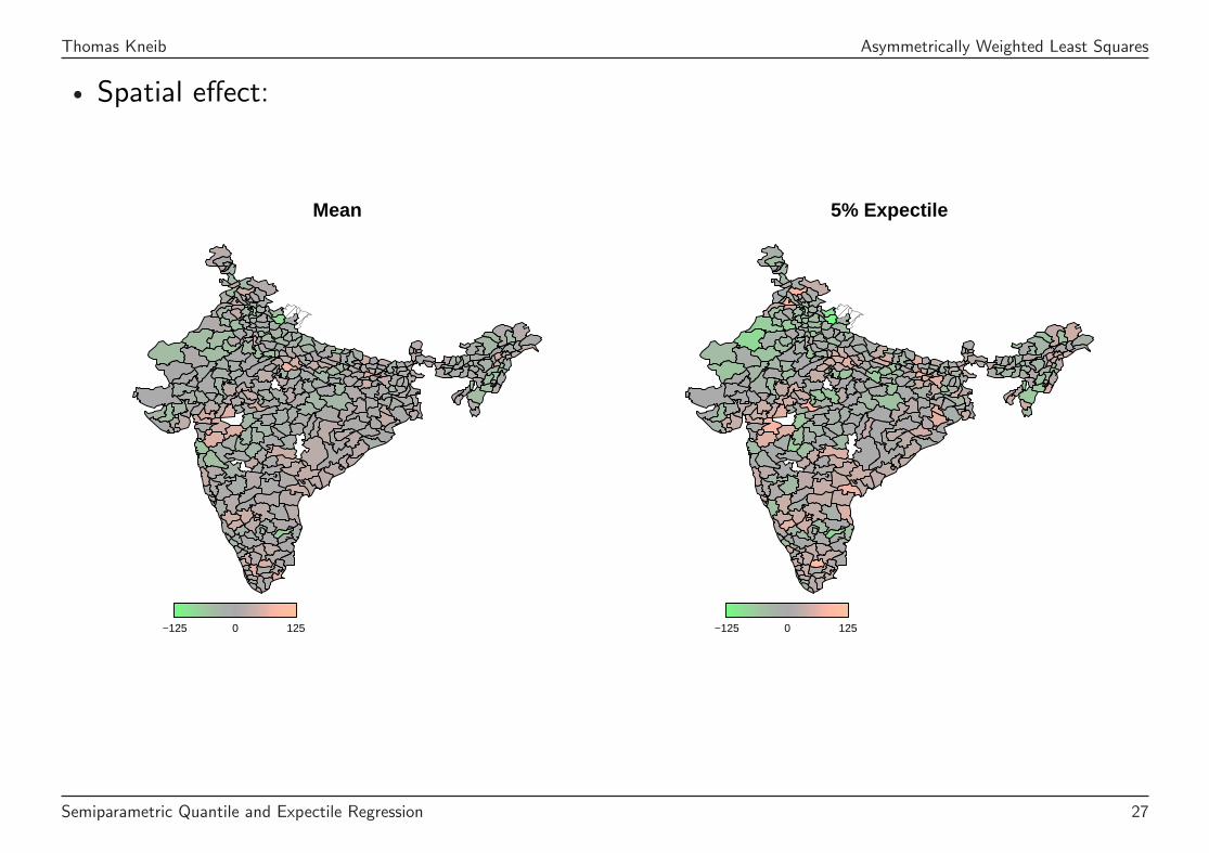
Thomas Kneib Asymmetrically Weighted Least Squares
• Spatial effect:
Mean
−125 1250
5% Expectile
−125 1250
Semiparametric Quantile and Expectile Regression 27

Thomas Kneib Boosting
Boosting
• Boosting yields a generic approach for both quantiles and expectiles.
• The estimation problem is formulated as an empirical risk minimisation problem:
n∑
i=1
wi(τ)|yi − ητi| → minητ
bzw.n∑
i=1
wi(τ)(yi − ητi)2 → minητ
• Main components of a boosting approach:
– A loss function defining the estimation problem.
– Suitable base-learning procedures for the model components.
• Estimation relies on the repeated application of the base-learning procedures tonegative gradients of the loss function (“residuals”).
Semiparametric Quantile and Expectile Regression 28
Thomas Kneib Boosting
• Componentwise boosting yields structured, interpretable model.
• Penalised least squares estimates yield suitable base-learners for semiparametricregression.
Semiparametric Quantile and Expectile Regression 29
Thomas Kneib Summary & Extensions
Summary & Extensions
• Flexible, semiparametric regression beyond mean regression.
• More complex models than in our example are possible, including for example
– interaction surfaces.
– random effects.
– different types of spatial effects.
• Different inferential procedures are available
– MCMC simulation techniques.
– Mixed Models.
– Boosting.
Semiparametric Quantile and Expectile Regression 30
Thomas Kneib Summary & Extensions
• Future work:
– Investigate properties of the statistical estimates resulting from quantile andexpectile regression
– In particular: How to perform inference for the estimated regression coefficients?
– Investigate properties of theoretical expectiles.
– Bayesian quantile regression based on flexible error distributions to avoid restrictiveassumptions on the error terms.
Semiparametric Quantile and Expectile Regression 31
Thomas Kneib Acknowledgements
Acknowledgements
• Location scale mixtures for Bayesian quantile regression: Yu Yue (Zicklin Schoolof Business, City University of New York), Elisabeth Waldmann (Department ofStatistics, LMU Munich), Stefan Lang (Department of Statistics, University ofInnsbruck).
• Expectile regression: Fabian Sobotka (Department of Mathematics, Carl von OssietzkyUniversity Oldenburg), Paul Eilers (University of Rotterdam), Sabine Schnabel (Max-Planck-Institute for Demography, Rostock).
• Boosting approaches: Nora Fenske, Torsten Hothorn (Department of Statistics, LMUMunich)
• A place called home:
http://www.staff.uni-oldenburg.de/thomas.kneib
Semiparametric Quantile and Expectile Regression 32


![Efficient Estimation in Expectile Regression Using ...[17] studied the sparse expectile regression under high dimensional settings where the penalty functions include the Lasso and](https://img.pdfslide.net/doc/110x75/5f029c6d7e708231d4052030/efficient-estimation-in-expectile-regression-using-17-studied-the-sparse-expectile.jpg)