Sensitivity analysis for randomised trials withmissing outcome data

Ian WhiteMRC Biostatistics Unit,Cambridge

15 September 2011UK Stata Users’ Group

MRC Biostatistics Unit 1/22

Motivation

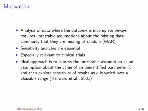
I Analysis of data where the outcome is incomplete alwaysrequires untestable assumptions about the missing data –commonly that they are missing at random (MAR)

I Sensitivity analyses are essential

I Especially relevant to clinical trials

I Ideal approach is to express the untestable assumption as anassumption about the value of an unidentified parameter δ,and then explore sensitivity of results as δ is varied over aplausible range (Kenward et al., 2001)

MRC Biostatistics Unit 2/22

Scope of the talk

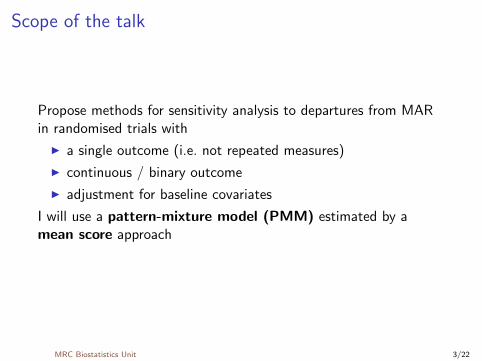
Propose methods for sensitivity analysis to departures from MARin randomised trials with

I a single outcome (i.e. not repeated measures)

I continuous / binary outcome

I adjustment for baseline covariates

I will use a pattern-mixture model (PMM) estimated by amean score approach

MRC Biostatistics Unit 3/22

Plan of the talk

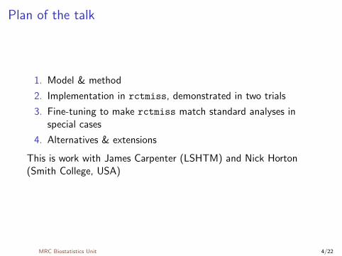
1. Model & method

2. Implementation in rctmiss, demonstrated in two trials

3. Fine-tuning to make rctmiss match standard analyses inspecial cases

4. Alternatives & extensions

This is work with James Carpenter (LSHTM) and Nick Horton(Smith College, USA)

MRC Biostatistics Unit 4/22

Analysis model

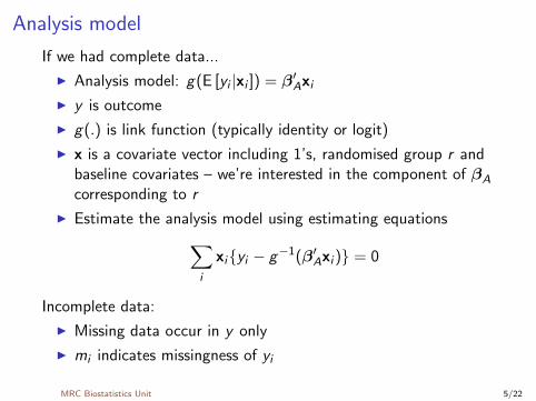
If we had complete data...

I Analysis model: g(E [yi |xi ]) = β′Axi

I y is outcome

I g(.) is link function (typically identity or logit)

I x is a covariate vector including 1’s, randomised group r andbaseline covariates – we’re interested in the component of βA

corresponding to r

I Estimate the analysis model using estimating equations

∑

i

xi{yi − g−1(β′Axi )} = 0

Incomplete data:

I Missing data occur in y only

I mi indicates missingness of yi

MRC Biostatistics Unit 5/22

Mean score approach: imputation model

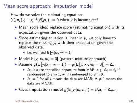
How do we solve the estimating equations∑i xi{yi − g−1(β′Axi )} = 0 when y is incomplete?

I Mean score idea: replace score (estimating equation) with itsexpectation given the observed data.

I Since estimating equation is linear in y , we only have toreplace the missing yi with their expectation given theobserved data.

I i.e. we need E [yi |xi ,mi = 1]

I Model E [yi |xi , mi = 0] (pattern mixture approach)I Assume g(E [yi |xi , mi = 1]) = g(E [yi |xi ,mi = 0]) + ∆i

I ∆i is a user-specified departure from MAR: e.g. ∆i = δ1 ifrandomised to arm 1, δ0 if randomised to arm 0.

I ∆i = 0 for all i means the data are MAR; ∆ 6= 0 means thedata are MNAR.

I Gives imputation model g(E [yi |xi , mi ]) = β′Ixi + ∆Iimi

MRC Biostatistics Unit 6/22

Mean score approach: estimation

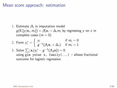
1. Estimate βI in imputation modelg(E [yi |xi , mi ]) = β′Ixi + ∆imi by regressing y on x incomplete cases (m = 0)

2. Form y∗i =

{yi if mi = 0g−1(βIxi + ∆i ) if mi = 1

3. Solve∑

i xi (y∗i − g−1(βAx)) = 0

using glm ystar x, family(...) – allows fractionaloutcome for logistic regression

MRC Biostatistics Unit 7/22

Mean score approach: variance

I Standard errors from glm ystar x, family(...) are toosmall – don’t allow for imputation of the y∗i

I We compute sandwich standard errors based on bothestimating equations:

SI (βA,βI ) =∑

i (1−mi )xi

{yi − g−1(β′Ixi )

}= 0

SA(βA, βI ) =∑

i xi

{y∗i (βI )− g−1(β′Axi )

}= 0

I Variance = B−1CB−T whereI B involves derivatives of (SA(β), SI (β)) with respect to

(βA, βI )I C involves sums of squares of score termsI both can be computed using matrix opaccum

MRC Biostatistics Unit 8/22

Strategy for sensitivity analysis

I Recall ∆ is the difference in g(E [yi |xi ,mi ]) between mi = 1and mi = 0

I If the main analysis assumed MAR (∆ = 0), we propose

1. sensitivity analysis assuming ∆i = δ for all individuals2. sensitivity analysis assuming ∆i = δ for all in intervention arm;

∆i = 0 for all in control arm3. sensitivity analysis assuming ∆i = δ for all in control arm;

∆i = 0 for all in intervention arm

over a range of δ that is plausible in the scientific context.

MRC Biostatistics Unit 9/22

QUATRO trial

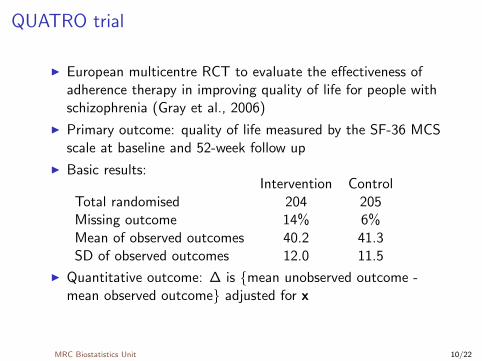
I European multicentre RCT to evaluate the effectiveness ofadherence therapy in improving quality of life for people withschizophrenia (Gray et al., 2006)

I Primary outcome: quality of life measured by the SF-36 MCSscale at baseline and 52-week follow up

I Basic results:Intervention Control

Total randomised 204 205Missing outcome 14% 6%Mean of observed outcomes 40.2 41.3SD of observed outcomes 12.0 11.5

I Quantitative outcome: ∆ is {mean unobserved outcome -mean observed outcome} adjusted for x

MRC Biostatistics Unit 10/22

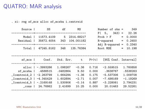
QUATRO: MAR analysis

. xi: reg sf_mcs alloc sf_mcsba i.centreid

Source | SS df MS Number of obs = 349

-------------+------------------------------ F( 5, 343) = 22.26

Model | 11573.4109 5 2314.68217 Prob > F = 0.0000

Residual | 35672.4054 343 104.001182 R-squared = 0.2450

-------------+------------------------------ Adj R-squared = 0.2340

Total | 47245.8162 348 135.76384 Root MSE = 10.198

--------------------------------------------------------------------------

sf_mcs | Coef. Std. Err. t P>|t| [95% Conf. Interval]

-------------+------------------------------------------------------------

alloc | -.3993286 1.098267 -0.36 0.716 -2.559515 1.760858

sf_mcsba | .4588515 .0482864 9.50 0.000 .3638767 .5538263

_Icentreid_2 | -2.263799 1.664294 -1.36 0.175 -5.537306 1.009708

_Icentreid_3 | -4.345429 1.602894 -2.71 0.007 -7.498169 -1.19269

_Icentreid_5 | -.2169148 1.530906 -0.14 0.887 -3.228061 2.794231

_cons | 24.76862 2.41699 10.25 0.000 20.01463 29.52261

--------------------------------------------------------------------------

MRC Biostatistics Unit 11/22

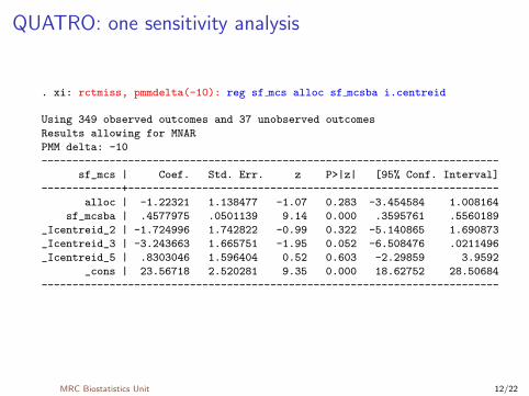
QUATRO: one sensitivity analysis

. xi: rctmiss, pmmdelta(-10): reg sf mcs alloc sf mcsba i.centreid

Using 349 observed outcomes and 37 unobserved outcomes

Results allowing for MNAR

PMM delta: -10

--------------------------------------------------------------------------

sf_mcs | Coef. Std. Err. z P>|z| [95% Conf. Interval]

-------------+------------------------------------------------------------

alloc | -1.22321 1.138477 -1.07 0.283 -3.454584 1.008164

sf_mcsba | .4577975 .0501139 9.14 0.000 .3595761 .5560189

_Icentreid_2 | -1.724996 1.742822 -0.99 0.322 -5.140865 1.690873

_Icentreid_3 | -3.243663 1.665751 -1.95 0.052 -6.508476 .0211496

_Icentreid_5 | .8303046 1.596404 0.52 0.603 -2.29859 3.9592

_cons | 23.56718 2.520281 9.35 0.000 18.62752 28.50684

--------------------------------------------------------------------------

MRC Biostatistics Unit 12/22

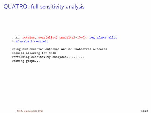
QUATRO: full sensitivity analysis

. xi: rctmiss, sens(alloc) pmmdelta(-10/0): reg sf mcs alloc

> sf mcsba i.centreid

Using 349 observed outcomes and 37 unobserved outcomes

Results allowing for MNAR

Performing sensitivity analyses...........

Drawing graph...

MRC Biostatistics Unit 13/22

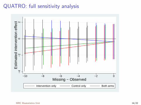
QUATRO: full sensitivity analysis

−4

−2

02

Est

imat

ed in

terv

entio

n ef

fect

−10 −8 −6 −4 −2 0Missing − Observed

Intervention only Control only Both arms

MRC Biostatistics Unit 14/22

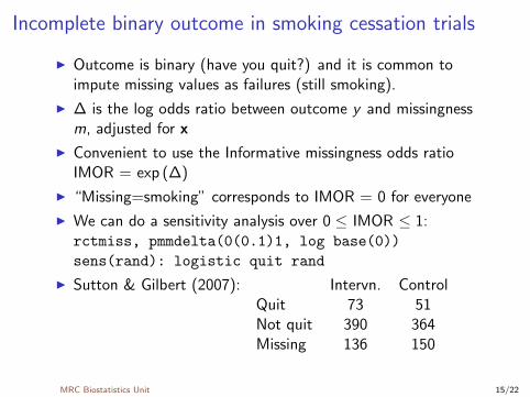
Incomplete binary outcome in smoking cessation trials

I Outcome is binary (have you quit?) and it is common toimpute missing values as failures (still smoking).

I ∆ is the log odds ratio between outcome y and missingnessm, adjusted for x

I Convenient to use the Informative missingness odds ratioIMOR = exp (∆)

I “Missing=smoking” corresponds to IMOR = 0 for everyone

I We can do a sensitivity analysis over 0 ≤ IMOR ≤ 1:rctmiss, pmmdelta(0(0.1)1, log base(0))sens(rand): logistic quit rand

I Sutton & Gilbert (2007): Intervn. ControlQuit 73 51Not quit 390 364Missing 136 150

MRC Biostatistics Unit 15/22

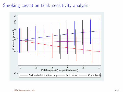
Smoking cessation trial: sensitivity analysis

.51

1.5

22.

53

Odd

s ra

tio fo

r ra

nd

0 .2 .4 .6 .8 1PMM exp(delta) in specified arm(s)

Tailored advice letters only both arms Control only

MRC Biostatistics Unit 16/22

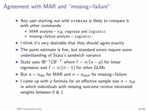
Agreement with MAR and “missing=failure”

I Any user starting out with rctmiss is likely to compare itwith other commands

I MAR analysis – e.g. regress and logisticI missing=failure analysis – logistic

I I think it’s very desirable that they should agree exactly

I The point estimate is fine, but standard errors require someunderstanding of Stata’s sandwich variance

I Stata uses fB−1CB−T where f = n/(n − p) for linearregression and f = n/(n − 1) for other GLMs

I But n = nobs for MAR and n = ntotal for missing=failure

I I came up with a formula for an effective sample size n = neff

in which individuals with missing outcome receive estimatedweights between 0 & 1

MRC Biostatistics Unit 17/22

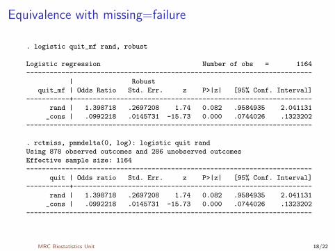
Equivalence with missing=failure

. logistic quit_mf rand, robust

Logistic regression Number of obs = 1164

-------------------------------------------------------------------------

| Robust

quit_mf | Odds Ratio Std. Err. z P>|z| [95% Conf. Interval]

-----------+-------------------------------------------------------------

rand | 1.398718 .2697208 1.74 0.082 .9584935 2.041131

_cons | .0992218 .0145731 -15.73 0.000 .0744026 .1323202

-------------------------------------------------------------------------

. rctmiss, pmmdelta(0, log): logistic quit rand

Using 878 observed outcomes and 286 unobserved outcomes

Effective sample size: 1164

-------------------------------------------------------------------------

quit | Odds ratio Std. Err. z P>|z| [95% Conf. Interval]

-----------+-------------------------------------------------------------

rand | 1.398718 .2697208 1.74 0.082 .9584935 2.041131

_cons | .0992218 .0145731 -15.73 0.000 .0744026 .1323202

-------------------------------------------------------------------------

MRC Biostatistics Unit 18/22

Equivalence with missing at random

. logistic quit rand, robust

Logistic regression Number of obs = 878

-------------------------------------------------------------------------

| Robust

quit | Odds Ratio Std. Err. z P>|z| [95% Conf. Interval]

--------+----------------------------------------------------------------

rand | 1.335948 .2626823 1.47 0.141 .9087009 1.964075

_cons | .1401099 .0209606 -13.14 0.000 .1045028 .1878494

-------------------------------------------------------------------------

. rctmiss, pmmdelta(0): logistic quit rand

Using 878 observed outcomes and 286 unobserved outcomes

Effective sample size: 877.99993

-------------------------------------------------------------------------

quit | Odds ratio Std. Err. z P>|z| [95% Conf. Interval]

--------+----------------------------------------------------------------

rand | 1.335948 .2626823 1.47 0.141 .9087008 1.964075

_cons | .1401099 .0209606 -13.14 0.000 .1045028 .1878494

-------------------------------------------------------------------------

MRC Biostatistics Unit 19/22

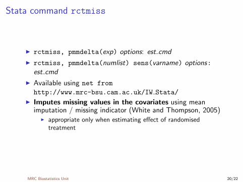
Stata command rctmiss

I rctmiss, pmmdelta(exp) options: est cmd

I rctmiss, pmmdelta(numlist) sens(varname) options:est cmd

I Available using net fromhttp://www.mrc-bsu.cam.ac.uk/IW Stata/

I Imputes missing values in the covariates using meanimputation / missing indicator (White and Thompson, 2005)

I appropriate only when estimating effect of randomisedtreatment

MRC Biostatistics Unit 20/22

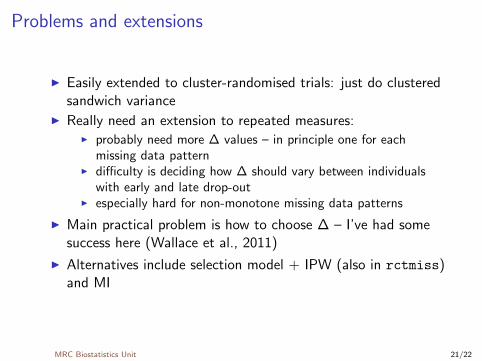
Problems and extensions

I Easily extended to cluster-randomised trials: just do clusteredsandwich variance

I Really need an extension to repeated measures:I probably need more ∆ values – in principle one for each

missing data patternI difficulty is deciding how ∆ should vary between individuals

with early and late drop-outI especially hard for non-monotone missing data patterns

I Main practical problem is how to choose ∆ – I’ve had somesuccess here (Wallace et al., 2011)

I Alternatives include selection model + IPW (also in rctmiss)and MI

MRC Biostatistics Unit 21/22

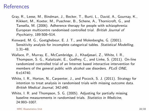
References

Gray, R., Leese, M., Bindman, J., Becker, T., Burti, L., David, A., Gournay, K.,Kikkert, M., Koeter, M., Puschner, B., Schene, A., Thornicroft, G., andTansella, M. (2006). Adherence therapy for people with schizophrenia:European multicentre randomised controlled trial. British Journal ofPsychiatry, 189:508–514.

Kenward, M. G., Goetghebeur, E. J. T., and Molenberghs, G. (2001).Sensitivity analysis for incomplete categorical tables. Statistical Modelling,1:31–48.

Wallace, P., Murray, E., McCambridge, J., Khadjesari, Z., White, I. R.,Thompson, S. G., Kalaitzaki, E., Godfrey, C., and Linke, S. (2011). On-linerandomized controlled trial of an Internet based interactive intervention formembers of the general public with alcohol use disorders. PLoS ONE,6:e14740.

White, I. R., Horton, N., Carpenter, J., and Pocock, S. J. (2011). Strategy forintention to treat analysis in randomised trials with missing outcome data.British Medical Journal, 342:d40.

White, I. R. and Thompson, S. G. (2005). Adjusting for partially missingbaseline measurements in randomised trials. Statistics in Medicine,24:993–1007.

MRC Biostatistics Unit 22/22