Sensitivity analysis for the outages of nuclear power plants

Energy SystDOI 10.1007/s12667-013-0096-y

ORIGINAL PAPER

Sensitivity analysis for the outages of nuclear powerplants

Kengy Barty · J. Frédéric Bonnans ·Laurent Pfeiffer

Received: 15 March 2012 / Accepted: 9 October 2013© Springer-Verlag Berlin Heidelberg 2013

Abstract Nuclear power plants must be regularly shut down in order to perform refu-eling and maintenance operations. The scheduling of the outages is the first problemto be solved in electricity production management. It is a hard combinatorial prob-lem for which an exact solving is impossible. Our approach consists in modelling theproblem by a two-level problem. First, we fix a feasible schedule of the dates of the out-ages. Then, we solve a low-level problem of optimization of electricity production, byrespecting the initial planning. In our model, the low-level problem is a deterministicconvex optimal control problem. Given the set of solutions and Lagrange multipliersof the low-level problem, we can perform a sensitivity analysis with respect to datesof the outages. The approximation of the value function which is obtained could beused for the optimization of the schedule with a local search algorithm.

Keywords Sensitivity analysis · Nuclear power plants · Optimal control ·Pontryagin’s principle

Mathematics Subject Classification (2000) 49K15 · 49K40 · 90C25

K. BartyEDF R&D, 1, avenue du Général de Gaulle, 92141 Clamart CEDEX, Francee-mail: [email protected]

J. F. Bonnans (B) · L. PfeifferEcole Polytechnique, CMAP & Inria Saclay, Route de Saclay, 91128 Palaiseau CEDEX, Francee-mail: [email protected]

L. Pfeiffere-mail: [email protected]

123

K. Barty et al.

1 Introduction

Energy generation in France is a competitive market, whereas transportation and dis-tribution are monopolies. Electric utilities generate electricity from hydro reservoirs,fossil energy (coal, gas), atom (nuclear fission process) and to a small extent from windfarms, solar energy or run of river plant without pondage. This energy mix providesenough power and flexibility to match energy demand in any circumstances. Hydropower stations are managed in order to remove peaks on the load curve during peak-hours, whereas thermal power stations supply base load energy. Due to their capacitygeneration and their production cost as well, the base load part is mainly supportedby nuclear power stations.

Nuclear facilities are subject to various constraints, and this induces a variationof the availability of nuclear energy. Some events may occur randomly during theoperating period and cause forced outages. This is why outages must be plannedby the producer in order to perform maintenance and refuelling operations of thefleet of nuclear power stations and in order to avoid a dramatical decrease of thenuclear availability. Thermal power stations, using expensive resources such as coalor gas, enable to compensate a lack of nuclear energy. These supplementary costs,due to the nuclear unavailability must be minimized when a schedule of the outagesis planned.

Each power station has its scheduling variables, which are submitted to localand coupling constraints as well. There are different constraints in the schedul-ing of outages of power plants: on the minimum spacing, on the maximum over-lapping between outages, and on the number of outages in parallel. For operat-ing purposes, the decision to stop a power station for maintenance has to be fore-cast far ahead. As a consequence, scheduling decisions are modelled as “open-loop” decisions, which means that they do not depend on the consumption sce-nario.

Given the planning of outages, the low-level problem of electricity production canbe described by a discrete time dynamic and stochastic optimization problem. Theoverall optimization problem is a large scale, mixed integer stochastic problem. Werefer to [2,5–7] for precise descriptions of this problem. At Electricité de France,the numerical resolution of this problem uses local search algorithms in order toimprove the current planned program. Numerous slight modifications are performedaround the current program and the most profitable determines the next program.The computational burden to solve this problem is heavy, reducing it is a challengingtask.

In this paper, we perform a sensitivity analysis of the electricity production problemwhen the integer parameters defining the scheduling of the outages are set. We providea first-order expansion of the value of this low-problem, with respect to the dates ofthe outages. For the sake of simplicity, the low-level problem is a convex deterministicoptimal control problem with continuous time. We do not consider the combinatorialside of the problem.

In the first section, we discuss the structure of solutions to the low-level problem,which are not unique in general. In the second section, we realize the sensitivityanalysis by using a well suited time reparameterization. We obtain a formula for the

123

Sensitivity analysis

directional derivatives of the value function using the opposite of the jumps of thetrue Hamiltonian at the times of beginning or end of the outages. It is based on theset of Lagrange multipliers, which we describe precisely. The result is an applicationof a theorem of [1]. The technical aspects related to the theorem such as the proof ofqualification or the proof of convergence of the solutions to the perturbed problemsare postponed in the third section.

2 Study of the reference problem

In this first part, we study the low-level problem of production management andtherefore consider that the dates of the outages are fixed. In our model, we onlyconsider one outage for each plant. Applying Pontryagin’s principle, we study theparticular structure of the optimal controls, which are not unique in general.

2.1 Notations, model and mathematical hypotheses

The main notations for the problem are the following:

[0, T ] the time periodc(x) the cost of production of an amountx

with thermal power stationsd(t) the demand of electricity at time td(t) the demand of electricity at time tS the set of nuclear power plantsn the number of nuclear power plantssi (t) the amount of available fuel of plant i at time tsi

0 the initial level of plant iui (t) the rate of production of plant i at time tui the maximum rate of production of plant i at time tU the set of controls defined by

{u ∈ Rn, such that ui ∈ [0, ui ], ∀i ∈ S}

τ ib the date of the beginning of the outage of plant i

τ ie the date of the end of the outage of plant i

T the set of dates defined by∪i∈S

{τ i

b, τie

}.

W (t) the set of working plants at time t,defined by W (t) = {

i ∈ S, t /∈ [τ ib, τ

ie ]}

ai (t) the rate of refuelling of plant i at time t,with ai (t) ≥ 0

φ(s(T )) a decreasing convex function of the final stateV (τb, τe) the value of the problem in function of τb and τe.

(1)

123

K. Barty et al.

The optimal control problem (P(τb, τe)) is

V (τb, τe) = minu,s

T∫

0

c(

d(t) −∑

i∈W (t)

ui (t))

dt + φ(s(T )),

s.t. ∀i ∈ S, si (t) = −ui (t) + ai (t)1[τ ib,τ i

e](t), for a. a. t,

0 ≤ ui (t) ≤ ui , for a. a. t,si (0) = si

0,

si (τ ib) = 0,

si (T ) ≥ 0,

(P(τb, τe))

where u ∈ L∞(0, T ; Rn) and s ∈ W 1,∞(0, T ; R

n).The dynamic of the stocks of fuel is clear from the differential equation: the stock

si decreases at rate ui (t) during the time period and increases at rate ai (t) during thetime of outage. The argument of the cost function c is the amount of energy which isnot produced with nuclear power plants in order to satisfy the demand. This energy isproduced with other types of power stations, which are more expensive. In our model,we also allow the total production to be greater than the demand.

Note that for optimal solutions, we will obtain that for all i in S, for almost all t in[τ i

b, τie ], the control ui (t) is equal to 0, see Lemma 1.

Mathematical hypotheses For our study, we suppose that the following hypothesesare satisfied:

– the cost functions c(x) and φ(s), the demand d(t) and the rate of refuelling a(t)are continuously differentiable functions,

– the cost function c(x) is strongly convex with parameter α on R,– the final cost function φ(s) is strictly convex on R

n+ and for all s in R

n+ , for all i

in S,

Dsi φ(s) < 0.

Feasibility of the problem The problem has a feasible control with a feasible tra-jectory associated if and only if, for all i in S,

τ ib · ui ≥ si

0.

Moreover, we can prove the existence of an optimal solution in this case. It followsfrom the boundedness of the controls and the convexity of the cost functions, seeLemma 8. In the sequel, we will assume that the following qualification condition issatisfied: for all i in S,

τ ib > 0, ui > 0, τ i

b · ui > si0, and

τ ie∫

τ ib

ai (t) dt > 0. (QC)

123


Note that this last integral is equal to si (τ ie ). This hypothesis will enable us to prove an

abstract qualification condition, needed to apply Pontryagin’s principle and to realizethe sensitivity analysis (see Lemma 9).

2.2 Study of the optimal controls

This subsection is dedicated to the study of an optimal control u(t), which minimizesthe Hamiltonian for almost all t . For our problem, the Hamiltonian has the particularityto be independent on the state s.

Let us denote by p the costate associated with s. Given a subset W of S, we definethe Hamiltonian of the system by

HW (t, u, p) = c(

d(t) −∑

i∈W

ui)

+∑

i∈S

pi(

− ui + ai (t)1i /∈W

)(2)

for t in [0, T ], u in U and p in Rn . The notation U has been introduced in (1). This

subscript W will be particularly useful later, since we will consider the Hamiltonianat times τ i

b and τ ie at which there are two sets of working plants of interest (one

includes the plant beginning or ending its outage, the other does not). Notice that theHamiltonian does not depend on the state s.

Proposition 1 (Pontryagin’s principle) If hypothesis (QC) holds, then for all optimalsolution (u, s), there exists a costate t �→ p(t) ∈ R

n such that for all i in S,

– pi (t) is a step function, taking two values pi (0) and pi (T ) on the intervals [0, τ ib)

and (τ ib, T ] respectively

– pi (T ) ≤ Dsi φ(s(T )) and pi (T ) = Dsi φ(s(T )) if si (T ) > 0

and such that for almost all t in [0, T ], the control minimizes the Hamiltonian:

HW (t)(t, u(t), p(t)

) = minv∈U

HW (t)(t, v, p(t)

). (3)

Proof In Lemma 9, we prove that hypothesis (QC) implies Robinson’s qualificationcondition (RQC). This condition enables us to apply Pontryagin’s principle for sys-tems with a final-state constraint, see [4, section 2.4.1, theorem 1] for a proof. Forour problem, each state variable si can be decomposed into two state variables, onedescribing the dynamic of the stock before its outage, one describing its dynamic after.This is why we can view the constraint s(τ i

b) = 0 as a final-state constraint. The costatep is a step function because nor the dynamic, neither the cost function depend on thestate. The discontinuity of the coordinate pi at time τ i

b is due to the state constraints(τ i

b) = 0. �

In the sequel, we will consider that a costate is an element of R2n which is charac-

terized by its values p(0) and p(T ) at times 0 and T . For all p = (p0, pT ) in R2n , we

associate the costate function defined by

123

K. Barty et al.

pi (t) ={

pi (0) if t ∈ [0, τ ib),

pi (T ) if t ∈ (τ ie , T ], ∀i ∈ S.

We assign no value to pi at time τ ib. However, we will use the following notation in

the sequel: if plant i is the only plant to start an outage at time t = τ ib, p(t−) and

p(t+) are such that for all j �= i ,

p j (t−) = p j (t+) = p j (t) (4)

and such that

pi (t−) = pi (0), and pi (t+) = pi (T ). (5)

Now, let us study the problem of minimization of the Hamiltonian introduced in (3).Let t ∈ [0, T ]\T (that is to say, t is different from all the dates of beginning or end ofoutage). Let u be an optimal solution and let p ∈ R

2n be an associated costate. Sincet /∈ T , p(t) and W (t) are uniquely defined. Note that if i /∈ W (t), then necessarilyt > τ i

b and thus

pi (t) = pi (T ) ≤ Dsi φ(s(T )) < 0. (6)

Consider the problem

minv∈U

c(

d(t) −∑

i∈W (t)

vi)

+∑

i∈S

pi (t)(

− vi + ai (t)1[τ ib,τ i

e](t)

). (Pt )

As we can see, the term∑

i∈ Spi (t)ai (t)1[τ i

b,τ ie](t) does not play any role here. More-

over, we can decompose the problem by introducing an additional variable μ for thetotal production, the sum

∑i∈W (t) vi . Let us set

UW (t) =∑

i∈W (t)

ui

and let us define, for μ in [0, UW (t)],

ξt (μ) = minv∈U ,∑

i∈W (t) vi =μ,

vi =0, ∀i /∈W (t)

∑

i∈W (t)

−pi (t)vi . (7)

Now, we can focus on the following one-dimensional problem:

min0≤μ≤UW (t)

c(d(t) − μ

) + ξt (μ). (P ′t )

123


The following Lemma justifies problem P ′t .

Lemma 1 If u is a solution to problem Pt , then∑

i∈Sui is a solution to problem P ′

tand ui = 0∀i /∈ W (t). Conversely, if μ is a solution to P ′

t , then there exists a solutionu to problem P ′

t which is such that∑

i∈ Sui = μ.

Proof Let u ∈ U be a solution to problem Pt . By (6), for all i /∈ W (t), −pi (t) > 0and thus ui = 0. It is then clear that μ = ∑

i∈ Sui = ∑

i∈W (t) ui is a solution to P ′t .

Conversely, let μ be a solution to P ′t . Since μ ≤ UW (t), the optimization problem (7)

is feasible and has a solution in U , say u, since U is compact. Then,∑

i∈Sui = μ and

it is easy to check that u is a solution to P ′t .

Problem P ′t has an economic interpretation. Producing at time t at a rate u has

a consequence on the dynamic of the state after time t . This is represented by thefunction ξt (μ). In some sense, the real numbers −p1(t), . . . ,−pn(t) are the marginalprices associated with the production at time t . Problem P ′

t takes into account boththe cost function c(d(t) − μ) and the cost of production ξt (μ).

Notations In the next three lemmas, we focus on problem P ′t . We always assume

that t is a given time in [0, T ]\T , u an optimal solution and p an associated costate.Let us denote by K the cardinal of {pi (t), i ∈ W (t)}. In the sequel, keep in mindthat it may be possible that pi (t) = p j (t) for some i and j in W (t). In this case, thecorresponding value pi (t) = p j (t) is counted only once and then K < |W (t)|. Weconsider the mapping σ from {1, . . . , K } to P(W (t)) (the power set of W (t)) uniquelydefined by:

(i)∀k ∈ {1, . . . , K }, ∀ i ∈ σ(k), ∀ j ∈ W (t), (p j (t) = pi (t)) ⇔ ( j ∈ σ(k)). (8)

This common value will be denoted by pk(t).

(i i)∀k, l ∈ {1, . . . , K }, k < l ⇒ pk(t) > pl(t). (9)

This mapping is nothing but a decreasing ordering of the coordinates of p(t) involvedin the definition of ξt . We also set, for k in {1, . . . , K },

Uk =k∑

l=1

∑

i∈σ(l)

ui (10)

and U0 = 0. Note that UK = UW (t). In the sequel, indexes i and j will be elements ofS and will appear at the top, whereas indexes k and l will be elements of {1, . . . , K }and will appear at the bottom.

The function μ �→ ξt (μ) is piecewise affine and convex. We make its value expliciton [0, UK ]:

⎧⎪⎪⎪⎨

⎪⎪⎪⎩

ξt (μ) = −p1(t)μ, ∀μ ∈ [0, U1],ξt (μ) = −p2(t)(μ − U1) + ξt (U1, ), ∀μ ∈ [U1, U2],

. . .

ξt (μ) = −pK (t)(μ − UK−1) + ξt (UK−1), ∀μ ∈ [UK−1, UK ].(11)

123

K. Barty et al.

The following Lemma shows that there is an ordering in the use of the fuel: webegin by using the power of the plants of greatest costate.

Lemma 2 Let i and j in W (t) be such that −pi (t) < −p j (t), if v is a solution to Pt ,then

(v j > 0) ⇒ (vi = ui ),

or, equivalently,

(vi < ui ) ⇒ (v j = 0).

Proof This is a direct consequence of Lemma 1 and the expression of ξt (μ) given by(11). �

The interpretation of the Lemma is the following: if −pi (t) < −p j (t), then plant iis cheaper than plant j at time t and should be used first. The next Lemma gives thenecessary optimality conditions of problem P ′

t .

Lemma 3 Problem P ′t has a unique solution on [0, UK ], say μ. The following four

cases hold true.

1. If there exists k in {1, . . . , K } such that μ ∈]Uk−1, Uk[, then

c′(d(t) − μ) = −pk(t). (12)

2. If there exists k in {0, . . . , K } such that μ = Uk, then(a) if k ∈ {1, . . . , K − 1},

− pk(t) ≤ c′(d(t) − Uk) ≤ −pk+1(t). (13)

(b) if k = 0,

c′(d(t) − 0) ≤ −p1(t). (14)

(c) and if k = K ,

− pK (t) ≤ c′(d(t) − UK ). (15)

Proof The function μ �→ c(d(t)−μ)+ξt (μ) is continuous and defined on a compactinterval, whence the existence of the solution. Furthermore, this function is strictlyconvex, since c is so. The uniqueness of the solution follows. For the optimalityconditions, we use the assumption of differentiability of c and the explicit formula ofξt (μ) given by (11). �

123


The goal of the next Lemma is to give a characterization of the solutions to problemP ′

t in function of d(t). We denote by kmin and kmax the smallest indices such that

limx→−∞ c′(x) < −pkmin and − pkmax < lim

x→+∞ c′(x) respectively.

For all k in {kmin, . . . , kmax}, we set

{d−

k = c′−1(−pk(t)) + Uk−1,

d+k = c′−1

(−pk(t)) + Uk .(16)

We also set

d+kmin−1

= −∞ and d−kmax+1 = +∞.

We have

d+kmin−1

< d−kmin < d+

kmin < d−kmin+1

< · · · < d−kmax < d+

kmax < d−kmax+1.

Now, we can express the optimal solution μ in function of d(t).

Lemma 4 The following two cases hold true.

1. If for some k in {kmin, . . . , kmax}, d−k ≤ d(t) ≤ d+

k , then

μ = d(t) − c′−1(−pk(t)),

ui = ui , ∀i ∈ σ(l), l < k,∑

i∈ σ(k)

ui = d(t) − c′−1(−pk(t)) − Uk−1,

ui = 0, ∀i ∈ σ(l), l > k.

2. If for some k in {kmin − 1, . . . , kmax}, d+k ≤ d(t) ≤ d−

k+1, then

μ = Uk,

ui = 0, ∀i ∈ σ(l), l > k,

ui = ui , ∀i ∈ σ(l), l ≤ k.

Proof Since the problem is convex, it suffices to check the necessary optimality con-ditions detailed in Lemma 3. For the first case, the condition satisfied is (12). In thesecond case, if k = 0, the satisfied condition is (14), if k = K , the satisfied conditionis (15), otherwise, the satisfied condition is (13). �Remark 1 In Lemma 4, we see that the coefficients d−/+

k play an important role,since they enable us to compute the optimal solutions to problem Pt . Keep in mindthat these coefficients depend on p(t). As a consequence, they have to be viewed asstep functions of time.

We state now a uniqueness property of the optimal controls.

123

K. Barty et al.

Lemma 5 Let (u1, s1) and (u2, s2) be two optimal solutions. Then, for almost all t in[0, T ], ∑i∈S

ui1(t) = ∑

i∈Sui

2(t) and s1(T ) = s2(T ).

Proof It is well-known that for a convex optimization problem, if the cost functionis strictly convex with respect to one of the optimization variables, then the value ofthis variable is unique at the optimum. For our problem, since c and φ are strictlyconvex, we have that

∑i∈W (t) ui

1(t) = ∑i∈W (t) ui

2(t) for almost all t in [0, T ] and

s1(T ) = s2(T ). Since u1(t) = u2(t) = 0 for almost all t in [τ ib, τ

ie ], we finally obtain

that∑

i∈Sui

1(t) = ∑i∈S

ui2(t) for almost all t . �

Remark 2 While the sum of the controls is unique, there may be several differentsoptimal controls. This happens when there are at least two plants i and j for whichpi (t) = p j (t) on a subinterval of [0, T ]. If the demand satisfies strictly the inequalitiesof the first case of Lemma 4, then the problem of minimization of the Hamiltonian, Pt ,has several optimal solutions and the general problem has equally, in general, severalsolutions.

3 Sensitivity analysis

3.1 Theoretical material

In this subsection, we state an abstract general theorem for the sensitivity analysis ofa convex problem. Consider the general parameterized problem

V (y) = minx∈X

f (x, y), subject to G(x, y) ∈ K , (Py)

in which y stands for the perturbation parameter and belongs to a space Y . The func-tions f and G are supposed to be continuously differentiable with respect to x and y.K is a closed convex subset of a space Z . The spaces X , Y and Z are Banach spaces.We fix a reference value y0 for y. Let x be a feasible point of the reference problemwith y = y0. We say that Robinson’s qualification condition holds at x if there existsε > 0 such that

εBZ ⊂ G(x, y0) + Dx G(x, y0)X − K , (RQC)

where BZ is the unit ball of Z . For λ in Z∗, we define the Lagrangian by

L(x, λ, y) = f (x, y) + 〈λ, G(x, y)〉.

In a general framework, for a solution x0 to the optimization problem with y = y0,the set of Lagrange multipliers (x0, y0) is defined by

(x0, y0) = {λ ∈ Z∗, Dx L(x0, λ, y0) = 0, λ ∈ NK (G(x0, u0)}, (17)

123


where NK (G(x0, u0) is the normal cone of K at G(x0, u0), defined by

NK (G(x0, u0)) = {λ ∈ Z∗, 〈λ, z − G(x0, u0)〉 ≤ 0, ∀z ∈ K }. (18)

We suppose now that the reference problem Py0 is convex, following [1, definition2.163]. Problems, like our application problem, with a convex cost function, linearequality constraints, and finite convex inequality constraints are convex. For a convexproblem, the set of Lagrange multipliers is the set of solutions of a dual problem whichdoes not depend on the choice of the (primal) solution x0. Therefore, (x0, y0) doesnot depend on x0 and we simply write (y0).

The following theorem establishes a differentiability property of the value func-tion of the problem V (y). See [1, definition 2.45] for a definition of the Hadamarddifferentiability.

Theorem 1 Consider a reference value y0. Suppose that:

1. Problem Py0 is convex and has a non-empty set of optimal solutions S(y0).2. Robinson’s qualification condition holds at all x0 in S(y0).3. For any sequence (yk)k converging to y0, for all k, problem Pyk possesses an

optimal solution xk such that, for all λ in (y0), for all sequence (y′k)k satisfying

y′k ∈ [y0, yk], one has:

Dy L(x0, λ, y0) is a limit point o f Dy L(xk, λ, y′k).

Then the optimal value function V is Hadamard directionally differentiable at y0 inany direction w and

V ′(y0, w) = inf sup Dy L(x, λ, y0)w.x∈S(y0) λ∈(y0)

(19)

This theorem is a direct extension of [1, theorem 4.24], which was originally provedin [3]. In the original formulation of the theorem, the third assumption is replaced bythe following assumption: for any sequence (yk)k converging to y0, for all k, problemPyk possesses an optimal solution xk such that the sequence (xk)k has a limit point inS(y0). However, this assumption would be rather painful to check for our problem, thisis why we prefer weakening it with this new assumption. Note also that the assumptionof convexity of the problem is essential for the sensitivity analysis. In a non-convexsetting, we would have to assume in addition that a certain sufficient second-ordercondition holds (see [1, theorems 4.25 and 4.65], for example).

Proof (Theorem 1) Let us adapt the proof given in [1]. Note first that since Robinson’squalification condition holds and since there exist optimal solutions, the set (y0) ofLagrange multipliers is nonempty and thus, the expression of the directional derivative(19) is finite. It is proved in [1, proposition 4.22] that under the directional regularitycondition, for any mapping α ∈ R+ �→ y(α) ∈ Y defined on a neighborhood of 0such that y(α) = y0 + αw + o(α) the following holds:

123

K. Barty et al.

lim supα↓0

V (y(α)) − V (y0)

α≤ inf sup

x∈S(y0) λ∈(y0)

Dy L(x, λ, y0)w. (20)

The directional regularity condition is implied by Robinson’s qualification condition,see [1, theorem 4.9].

Let αn ↓ 0, let yn = y0 + αnw + o(αn) and let (xn)n be the sequence of solutionssuch that hypothesis (3) of the theorem is satisfied. Extracting a subsequence if nec-essary, we can suppose that (xn)n converges to x0 in S(y0). Let λ be in (y0). Since(y0) ⊂ NK (G(x0, y0)), and then

〈λ, G(xn, yn) − G(x0, y0)〉 ≤ 0,

we have

f (xn, yn) − f (x0, y0) ≥ L(xn, λ, yn) − L(x0, λ, y0).

By convexity of Py0 , the first order optimality conditions imply that x0 belongs toarg minx∈X L(x, λ, y0), and then

L(xn, λ, y0) ≥ L(x0, λ, y0). (21)

Since V (yn) = f (xn, yn) and by the mean value theorem and continuity of L(x, λ, y),we obtain from (21) that, for some y′

n in [y0, yn],V (yn) − V (y0) ≥ L(xn, λ, yn) − L(xn, λ, y0)

= αn Dy L(xn, λ, y′n)w

= αn Dy L(x0, λ, y0)w + o(αn),

since by assumption,

Dy L(xn, λ, y′n) → Dy L(x0, λ, y0).

As a consequence, since λ was arbitrary,

lim infn→∞

V (yn) − V (y0)

αn≥ sup

λ∈(y0)

Dy L(x0, λ, y0)

≥ inf supx∈S(y0) λ∈(y0)

Dy L(x, λ, y0)w. (22)

Combining (20) and (22), we obtain that for any y(α) = y0 + αw + o(α),

limα↓0

V (y(α)) − V (y0)

α= inf sup

x∈S(y0) λ∈(y0)

Dy L(x, λ, y0)w,

as was to be proved. �

123


3.2 Expression of the directional derivatives

In this subsection, we give a sensitivity formula for problem (P(τb, τe)). We showthat the value function is Hadamard directionally differentiable if all the dates ofthe outages are different. When differentiating the value function with respect to onevariable, the result obtained is the jump of the reduced Hamiltonian at the referencetime of the variable.

Time reparameterization Theorem 1 cannot be applied directly to our applicationproblem. Indeed, in its formulation, the cost function and the dynamic are not contin-uously differentiable with respect to τb and τe. For example, if we try to differentiatethe cost function with respect to the variable τ

je , we obtain the following derivative,

c

(

τj

e , d(τ

je

)−∑

i∈W

ui(τ

je

))

− c

⎛

⎝τj

e , d(τ

je

)−

∑

i∈W∪{ j}ui(τ

je

)⎞

⎠,

where W is the set of working plants at time τj

e ( j being excluded of W ). Thisexpression does not make sense, since the control is only in L∞(0, T ; R

n), thus, wecannot define its value at time τ

je .

However, if we perform a well suited change of variable in time, we can apply theabstract result. The change of variable that we use can be realized if and only if thefollowing hypothesis holds:

For all i and j in S such that i �= j, τ ib �= τ

jb , τ i

e �= τj

e and τ ib �= τ

je . (H)

We begin by computing Dτ

je

V (τb, τe). We consider a nuclear power plant j and

we denote by τ0 the reference value of τj

e and by (u, s) a solution with a costate p,for the reference problem with τ

je = τ0. As a consequence of (H), we get :

None of the plants, except j, begins or ends i ts outage at time τ0.

Let us consider two times t1 and t2 such that t1 < τ0 < t2 and such that they aresufficiently close to τ0 so that none of the plants (except j) begins or ends an outageduring [t1, t2]. The idea of the change of variable is to fix the time of the discontinuitydue to the end of the outage. We set, for all t ′ in [0, T ],

θτ

je(t ′) =

⎧⎪⎪⎨

⎪⎪⎩

t1 + τj

e −t1τ0−t1

(t ′ − t1), if t ′ ∈ [t1, τ0]t2 − t2−τ

je

t2−τ0(t2 − t ′), if t ′ ∈ [τ0, t2]

t ′, otherwise.

(23)

We perform the change of variable t = θτ

je(t ′). See Fig. 1 for an illustration of

the change of variable. It is well defined for τj

e in (t1, t2). We denote by W the set of

123

K. Barty et al.

Fig. 1 Change of variableassociated with the perturbation

of τj

e

working plants on the interval [t1, t2]. By convention, j does not belong to W . Thenew optimal control problem (P ′(τ j

e )) to be solved is

V (τj

e ) = minu,s

⎡

⎣t1∫

0

c

⎛

⎝d(t ′) −∑

i∈W (t ′)ui (t ′)

⎞

⎠ dt ′

+ τj

e −t1τ0−t1

τ0∫

t1

c

(

d ◦ θτ

je(t ′) −

∑

i∈W

ui (t ′))

dt ′

+ t2−τj

et2−τ0

t2∫

τ0

c

⎛

⎝d ◦ θτ

je(t ′) −

∑

i∈W∪{ j}ui (t ′)

⎞

⎠ dt ′

+T∫

t2

c

⎛

⎝d(t ′) −∑

i∈W (t ′)ui (t ′)

⎞

⎠ dt ′ + φ(s(T ))

⎤

⎦ ,

s.t. ∀i ∈ S, si (t ′) = . . .⎧⎪⎪⎪⎨

⎪⎪⎪⎩

τj

e −t1τ0−t1

[−ui (t ′) + ai ◦ θ

τj

e(t ′)1i /∈W

], if t ′ ∈ [t1, τ0],

t2−τj

et2−τ0

[−ui (t ′) + ai ◦ θ

τj

e(t ′)1i /∈W∪{ j}

], if t ′ ∈ [τ0, t2],

−ui (t ′) + ai (t ′)1[τ ib,τ i

e ](t ′), otherwise,

0 ≤ ui (t ′) ≤ ui ,

si (0) = si0,

si(τ i

b

) = 0,

si (T ) ≥ 0.

(P ′(τ je ))

It is easy to check that problems (P(τb, τe)) and (P ′(τ je )) have the same value when

τj

e belongs to (t1, t2). Since for all t ′ in [0, T ], θτ0(t′) = t ′, the original and the

reparameterized problems are the same for τj

e = τ0.

123


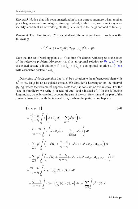
Remark 3 Notice that this reparameterization is not correct anymore when anotherplant begins or ends an outage at time τ0. Indeed, in this case, we cannot anymoreidentify a constant set of working plants ( j let alone) in the neighborhood of time τ0.

Remark 4 The Hamiltonian H ′ associated with the reparameterized problem is thefollowing:

H ′(t ′, u, p) = θτ

je(t ′)HW (t ′)(θτ

je(t ′), u, p).

Note that the set of working plants W (t ′) at time t ′ is defined with respect to the datesof the reference problem. Moreover, (u, s) is an optimal solution to P(τb, τe) withassociated costate p if and only if (u ◦ θ

τj

e, s ◦ θ

τj

e) is an optimal solution to P ′(τ j

e )

with associated costate p ◦ θτ

je

.

Derivation of the Lagrangian Let (u, s) be a solution to the reference problem withτ

je = τ0, let p be an associated costate. We consider a Lagrangian on the interval

[t1, t2], where the variable τj

e appears. Note that p is constant on this interval. For thesake of simplicity, we write p instead of p(t ′) and t instead of t ′. In the followingLagrangian, we only take into account the part of the cost function and the part of thedynamic associated with the interval [t1, t2], where the perturbation happens.

L(

u, s, p, τj

e

)(24)

= τj

e − t1τ0 − t1

τ0∫

t1

c

(

d ◦ θτ

je(t) −

∑

i∈W

ui (t)

)

dt

+ t2 − τj

e

t2 − τ0

t2∫

τ0

c

⎛

⎝d ◦ θτ

je(t) −

∑

i∈W∪{ j}ui (t)

⎞

⎠ dt

+∑

i∈S

pi

τ0∫

t1

(− si (t) + τ − t1

τ0 − t1(−ui (t) + ai ◦ θ

τj

e(t)1i /∈W )

)dt

+∑

i∈S

pi

t2∫

τ0

(−si (t) + τ − t2

τ0 − t2(−ui (t) + ai ◦ θ

τj

e(t)1i /∈(W∪{ j}))

)dt

= τj

e − t1τ0 − t1

τ0∫

t1

HW (t)(θτj

e(t), u(t), p) dt

+ t2 − τj

e

t2 − τ0

t2∫

τ0

HW (t)

(θτ

je(t), u(t), p

)dt −

∑

i∈S

t2∫

t1

pi si (t) dt.

123

K. Barty et al.

Before deriving the Lagrangian, let us introduce some notations. We define the trueHamiltonian by

H∗W (t, p) = min

vi ∈[0,ui ]HW (t, v, p), ∀p ∈ R

n . (25)

Pontryagin’s principle states that

H∗W (t)(t, p) = HW (t)(t, u(t), p), for a. a. t in [0, T ].

Note that the function t �→ H∗W (t)(t, u, p) is discontinuous at times τ i

e and τ ib, for all

i . Indeed, the set of working plants W (t) is changing precisely at these times. Thenext Lemma is a classic useful consequence of Pontryagin’s principle. See [4, section2.4.1, equality (8a)] for a proof.

Lemma 6 Let u be an optimal control, with associated costate p. Consider an interval(ta, tb) included in [0, T ] on which none of the plants begins or ends an outage. Onsuch an interval, the costate is constant and the set of working plants is constant, equalto say W . The mapping:

h : t ∈ [ta, tb] → H∗W (t, p)

is C1 on [ta, tb] and its derivative is given by

h(t) = Dt H∗W (t, p0) = Dt HW (t, u(t), p), f or a. a. t in [ta, tb], (26)

where the notation Dt HW stands for the partial derivative of HW with respect to t .

Note that this result can also be obtained by applying Theorem 1. Indeed, H∗W is

the value of an optimization problem (the minimization of the Hamiltonian), parame-terized by t . Since the constraints (u ∈ U) are unchanged, the derivative of H∗

W (t, p)

is the derivative of the cost function, here the Hamiltonian.

Proposition 2 The mapping τj

e �→ L(u, s, p, τj

e ) is differentiable on (t1, t2) and

Dτ

jeL(u, s, p, τ0) = H∗

W (τ0, p) − H∗W∪{ j}(τ0, p). (27)

Proof We have

Dτ

jeL(

u, s, p, τj

e

)=

[ 1

τ0 − t1

τ0∫

t1

HW (θτ

je(t), u(t), p) dt

+ τj

e − t1τ0 − t1

τ0∫

t1

t − t1τ0 − t1

Dt HW (θτ

je(t), u(t), p) dt

]

123


−[ 1

t2 − τ0

t2∫

τ0

HW∪{ j}(θτj

e(t), u(t), p) dt

− t2 − τj

e

t2 − τ0

t2∫

τ0

t2 − t

t2 − τ0HW∪{ j}

(θτ

je(t), u(t), p

)dt].

For τj

e = τ0, we obtain

Dτ

jeL(u, s, p, τ0) (28)

= 1

τ0 − t1

[ τ0∫

t1

H∗W (t, p) dt +

τ0∫

t1

(t − t1)Dt H∗W (t, p) dt

]

− 1

t2 − τ0

[ t2∫

τ0

H∗W∪{ j}(t, p) dt −

t2∫

τ0

(t2 − t)Dt H∗W∪{ j}(t, p) dt

].

Then, we obtain by integrating by parts (with Lemma 6)

τ0∫

t1

(t − t1)Dt H∗W (t, p) dt (29)

=[(t − t1)H∗

W (t, p)]τ0

t1−

τ0∫

t1

H∗W (t, p) dt

= (τ0 − t1)H∗W (τ0, p) −

τ0∫

t1

H∗W (t, p) dt,

and a similar expression holds for the integral on [τ0, t2]. Finally, we obtain

Dτ

jeL(u, s, p, τ0) = −

[H∗

W∪{ j}(τ0, p) − H∗W (τ0, p)

], (30)

as was to be proved. �

Remark 5 In general, there are several solutions to the problem. However, the expres-sion obtained for the derivative of the Lagrangian, when p is given, does not dependon the primal solution, for two reasons:

– the Hamiltonian, and thus the true Hamiltonian, do not depend on the state (andtherefore, they do not depend on the past trajectory)

123

K. Barty et al.

– by definition, the true Hamiltonian at time t does not depend on the choice of thevalue of the optimal control at time t .

Sensitivity with respect to the beginning of outage The above analysis remains truefor τ

jb if hypothesis (H) always holds. In this case, none of the plants (except j) begins

or stops its outage at time τj

b and we denote by W the set of working plants at thereference time τ0 ( j does not belong to W ). The only difference with the previousexpression is that the j th coordinate of p has a jump at time τ0. Using the conventions(4) and (5), we obtain the expression

Dτ

jbL(u, s, p, τ0) = −

[H∗

W

(τ0, p

(τ+

0

)) − H∗W∪{ j}

(τ0, p

(τ−

0

))]. (31)

Notice that the state constraint s j (τj

b ) = 0 has become s j (τ0) = 0, as a consequence,

it does not depend on τj

b anymore and we do not need to take it into account in theLagrangian.

Sensitivity with respect to an arbitrary direction We compute now the value of thedirectional derivative of the value function in an arbitrary direction. To this purpose,we must realize a complete reparameterization of the problem and some notations areneeded. We fix a reference value (τb,0, τe,0) for the dates of outages and we supposethat hypothesis (H) holds. Then, we can fix dates t i

b,1, t ib,2, t i

e,1 and t ie,2 in [0, T ] such

that for all i in S,

t ib,1 < τ i

b,0 < t ib,2 < t i

e,1 < τ ie,0 < t i

e,2

and such that on the intervals [t ib,1, t i

b,2] and [t ie,1, t i

e,2], plant i is the only one to begin

or to end its outage. Therefore, we can define the sets W ib and W i

e of working plantson the intervals [t i

b,1, t ib,2] and [t i

e,1, t ie,2] respectively, i being excluded of these sets.

The global change of variable to perform is now the following:

θτb,τe (t′) =

⎧⎪⎪⎪⎪⎪⎪⎪⎪⎪⎪⎪⎪⎪⎨

⎪⎪⎪⎪⎪⎪⎪⎪⎪⎪⎪⎪⎪⎩

t ib,1 + τ i

b−t ib,1

τ ib,0−t i

b,1

(t ′ − t i

b,1

), for t ′ in

[t ib,1, τ

ib,0

],

t ib,2 − t i

b,2−τ ib

t ib,2−τ i

b,0

(t ib,2 − t ′

), for t ′ in

[τ i

b,0, t ib,2

],

t ie,1 + τ i

e−t ie,1

τ ie,0−t i

e,1

(t ′ − t i

e,1

), for t ′ in

[t ie,1, τ

ie,0

],

t ie,2 − t i

e,2−τ ie

t ie,2−τ i

e,0

(t ie,2 − t ′

), for t ′ in

[τ i

e,0, t ie,2

],

t ′, otherwise.

(32)

123


The general reparameterized problem is the following:

V (τb, τe)

= minu,s

[ T∫

0

θτb,τe (t′) c

(d ◦ θτb,τe (t

′) −∑

i∈W (t ′)ui (t ′)

)dt ′ + φ(s(T ))

],

s.t. ∀i ∈ S,

si (t ′) = θτb,τe (t′)( − ui (t ′) + ai ◦ θτb,τe (t

′)1[τ i

b,0,τ ie,0

](t ′))

0 ≤ ui (t ′) ≤ ui ,

si (0) = si0,

si(τ i

b,0

)= 0,

si (T ) ≥ 0.

(P ′(τb, τe))

Here, the set of working plants W (t ′) at time t ′ is defined by:

W (t ′) ={

i ∈ S, t ′ /∈[τ i

b,0, τie,0

]}.

Notations Let us introduce some notations in order to simplify our sensitivity for-mula. First, we denote by �(τb,0, τe,0) the set of costates satisfying Pontryagin’sprinciple (Lemma 1) for the value (τb,0, τe,0) of the dates of the outages. Recall thatit is a subset of R

2n . We also introduce the jumps of the true Hamiltonian, denoted by�Hi

b(p) and �Hie (p) and defined by

�Hib(p) = H∗

W ib

(τ i

b,0, p(τ i +

b,0

))− H∗

W ib∪{i}

(τ i

b,0, p(τ i −

b,0

)),

�Hie (p) = H∗

W ie∪{i}

(τ i

e,0, p(τ i

e,0

))− H∗

W ie

(τ i

e,0, p(τ i

e,0

)),

for p in �(τb,0, τe,0).

Theorem 2 Consider a direction of perturbation denoted by (δτb, δτe). If hypothesis(H) holds, then

V ′((τb,0, τe,0), (δτb, δτe))

(33)

= supp∈�(τb,0,τe,0)

[ ∑

i∈S

−δτ ib�Hi

b(p) +∑

i∈S

−δτ ie�Hi

e (p)

].

Proof The expression of the derivative of the Lagrangian given in the thorem is asimple extension of expressions (27) and (31). The theorem is a direct consequenceof Theorem 1. For our application problem, a costate is a Lagrange multiplier if andonly if it satisfies Pontryagin’s principle, since the Hamiltonian is convex. The threehypotheses of the theorem (existence of solutions, qualification and continuity of thederivative of the Lagrangian) are checked in Lemmas 8, 9, and 14. �

123

K. Barty et al.

3.3 Study of the Lagrange multipliers

In this part, we give a complete description of the set �(τb, τe) of costates satisfy-ing Pontryagin’s principle, which is for our application problem the set of Lagrangemultipliers introduced in (17). Note that the characterization of costates holds even ifhypothesis (H) is not satisfied.

Notations Let us consider the smallest sequence of times

0 = τ0 < τ1 < · · · < τM = T

such that the outages begin or end only at times {τ1, . . . , τM }. For all integer m with0 ≤ m < M , the set of working plants is constant on the interval of time (τm, τm+1).

Let us fix now an optimal control u and its associated trajectory s. Since the set ofLagrange multipliers does not depend on the choice of the optimal solution, it sufficesto compute the set of costates associated with the particular solution (u, s). We haveproved in Lemma 5 that μ = ∑

i∈Sui (t) and s(T ) are unique. Let us define, for all i

in S,

⎧⎪⎪⎨

⎪⎪⎩

πi,min0 = ess sup

t∈[0,τ ib],ui (t)>0

{−c′(d(t) − μ(t))},

πi,max0 = ess inf

t∈[0,τ ib],ui (t)<ui

{−c′(d(t) − μ(t))}. (34)

For all i in S, if si (T ) > 0, we set

πi,minT = π

i,maxT = Dsi φ(s(T )) (35)

otherwise, we set

⎧⎪⎪⎪⎨

⎪⎪⎪⎩

πi,minT = ess sup

t∈[τ ie ,T ],ui (t)>0

{−c′(d(t) − μ(t))},

πi,maxT = min

{

ess inft∈[τ i

e ,T ],ui (t)<ui{−c′(d(t) − μ(t))}, Dsi φ(s(T ))

}

.

(36)

Theorem 3 The set of costates �(τb, τe) is described by

�(τb, τe) =(∏

i∈S

[π

i,min0 , π

i,max0

])

×(∏

i∈S

[π

i,minT , π

i,maxT

])

. (37)

Proof Let t in [0, T ], let v in U be such that for all i /∈ W (t), vi = 0. We setμ = ∑

i∈Svi . Fix q in R

n . Then v is a solution to the problem of minimization of theHamiltonian Pt with p = q if and only if for all i in W (t),

123


(vi > 0 ⇒ qi (t) ≥ −c′(d(t) − μ)

), (38)

(vi < ui ⇒ qi (t) ≤ −c′(d(t) − μ)

), (39)

and i /∈ W (t) ⇒ qi ≤ 0. (40)

Therefore, a costate p is such that the Hamiltonian is minimized for almost all t ifand only if conditions (38) and (39) are satisfied for almost all t with q = p(t).These conditions being inequalities, it suffices to consider the essential infimum andsupremum as we did in the construction of π

i,min0 , π i,max

0 , π i,minT and π

i,maxT . Notice that

we do not need to impose that pi (T ) ≤ 0, since we already have that Dsi φ(s(T )) ≤ 0.The theorem follows. �

The following Lemma describes situations where the costate is unique.

Lemma 7 Let us consider four different cases.

1. (a) If on a non-negligible subset of [0, τ ib], ui (t) ∈ (0, ui ), then pi (0) is unique.

(b) If si (T ) > 0 or if on a non-negligible subset of [τ ie , T ], ui (t) ∈ (0, ui ), then

pi (T ) is unique.2. (a) If there exist two non-negligible subsets T1 and T2 of a given interval [τm, τm+1]

with τm+1 ≤ τ ib such that

∀t ∈ T1, ui (t) = 0 and ∀t ∈ T2, ui (t) = ui ,

then, pi (0) is unique.(b) If the same property holds on an interval [τm, τm+1] with τm ≥ τ i

e , then pi (T )

is unique.

Proof In cases 1.a and 1.b, it follows from the existence of a non-negligible subsetof [0, τ i

b] (resp. [τ ie , T ]) where 0 < ui (t) < ui that π

i,min0 ≥ π

i,max0 (resp. π

i,minT ≥

πi,maxT ), whence the equality of these bounds and the uniqueness of pi (0) (resp. pi (T )).

For case 2.a, let us define rmin and rmax by

rmin = ess supt∈[τm ,τm+1],ui (t)>0

{−c′(d(t) − μ(t))},

rmax = ess inft∈[τm ,τm+1],ui (t)<ui

{−c′(d(t) − μ(t))}.

Clearly,

−∞ < rmin ≤ πi,min0 ≤ π

i,max0 ≤ rmax < +∞.

Let us show the uniqueness by contradiction. We suppose that πi,max0 − π

i,min0 =

ε > 0. It can be observed from Lemma 4 that the solution μ of problem P ′t depends

continuously on d(t) on the interval [τm, τm+1], since the set of working plants remains

123

K. Barty et al.

constant. The demand d(t) being continuous in time, it follows that c′(d(t) − μ(t)) isa continuous function of time. Let t1 and t2 be two times such that

− c′(d(t1) − μ(t1)) ≤ rmin + ε

3,

− c′(d(t2) − μ(t2)) ≥ rmax − ε

3.

The function c′(d(t)−μ(t)) being continuous, there exists a non-negligible subintervalof [t1, t2] (or [t2, t1] if t2 < t1) where −c′(d(t)−μ(t)) belongs to [rmin +ε/3, rmax −ε/3]. On this subinterval, there exists a non-negligible subset where either 0 < ui (t) <

ui , either ui (t) = 0 or ui (t) = ui . In the first case, we obtain the uniqueness of pi (0),which contradicts the statement of non-uniqueness. In the second case, we obtain that

ess inft∈[τm ,τm+1],ui (t)<ui

{−c′(d(t) − μ(t))} ≤ rmax − ε

3, (41)

and in the third case, we obtain that

ess supt∈[τm ,τm+1],ui (t)>0

{−c′(d(t) − μ(t))} ≥ rmin + ε

3, (42)

Inequalities (41) and (42) contradict the definition of rmin and rmax. Thus, pi (0) isunique. Case 2.b can be treated similarly. �

It follows from the contraposition of Lemma 7 that if for some i in S, pi (0) isnot unique, then the optimal control ui is constant on each interval (τm, τm+1) withτm+1 ≤ τ i

b, being equal to 0 or ui . Denoting by M0 the set of indexes m for whichui (t) = ui on (τm, τm+1), we obtain that

si0 = ui ·

∑

m∈M0

τm+1 − τm . (43)

Similarly, if pi (T ) is not unique, then si (T ) = 0 and the optimal control ui is constanton each interval (τm, τm+1) with τm ≥ τ i

e , being equal to 0 or ui . Denoting by MT theset of indexes m for which ui (t) = ui on (τm, τm+1), we obtain that

τ ie∫

τ ib

ai (t) dt = ui ·∑

m∈MT

τm+1 − τm . (44)

Inequalities (43) and (44) are, in some sense, unstable.

123


4 Technical aspects

In this part, we adopt some new notations in order to simplify the proofs. We set

�(t, u) = c

⎛

⎝d(t) −∑

i∈W (t)

ui

⎞

⎠,

and for a sequence of dates (τb,k, τe,k)k , we denote by θk the associated changes ofvariable, defined by (32) and we obtain, with the new notations:

V (τb,k, τe,k) = minu,s

T∫

0

θk(t) �(θk(t), u(t)) dt + φ(s(T )),

s.t. ∀i ∈ S, si (t) = θk(t)(−ui (t) + ai ◦ θk(t)1[τ i

b,0,τ ie,0](t)

),

0 ≤ ui (t) ≤ ui (t),si (0) = si

0,

si(τ i

b,0

)= 0,

si (T ) ≥ 0.

(P ′(τb, τe))

Let us give two elementary properties associated with the changes of variable θk .First, it can be easily checked that

θk → Id and θk → 1, (45)

for the uniform topology of L∞(0, T ; Rn). Moreover, if b is in L1(0, T ; R

n), then

b ◦ θk → b, (46)

for the L1-topology. This property being easily checked if b is continuous, by densityof continuous functions in L1(0, T ; R

n), we obtain it for all function in L1(0, T ; Rn).

4.1 Existence of solutions

Lemma 8 If condition (QC) is satisfied, the problem has an optimal solution.

Proof Consider a minimizing sequence (uk, sk) of feasible solutions. Since the con-trols are bounded and the dynamic is linear, one can easily prove with the Banach–Alaoglu theorem and the Arzelà–Ascoli theorem the existence of a subsequence(uk, sk) such that uk converges to a control u for the weak topology of L∞(0, T ; R

n),such that sk converges to a trajectory s for the strong topology of L∞(0, T ; R

n), andsuch that (u, s) is a feasible trajectory. Moreover, the mapping

123

K. Barty et al.

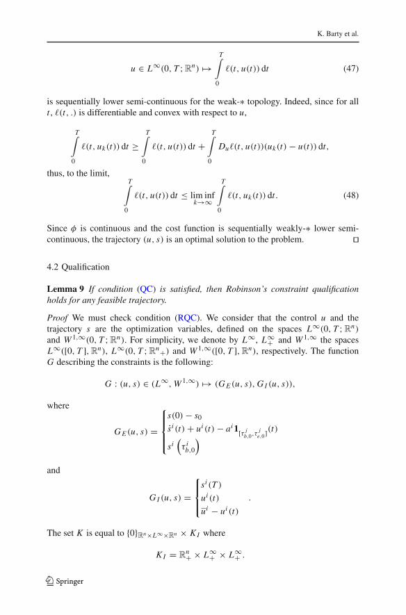
u ∈ L∞(0, T ; Rn) �→

T∫

0

�(t, u(t)) dt (47)

is sequentially lower semi-continuous for the weak-∗ topology. Indeed, since for allt , �(t, .) is differentiable and convex with respect to u,

T∫

0

�(t, uk(t)) dt ≥T∫

0

�(t, u(t)) dt +T∫

0

Du�(t, u(t))(uk(t) − u(t)) dt,

thus, to the limit,T∫

0

�(t, u(t)) dt ≤ lim infk→∞

T∫

0

�(t, uk(t)) dt. (48)

Since φ is continuous and the cost function is sequentially weakly-∗ lower semi-continuous, the trajectory (u, s) is an optimal solution to the problem. �

4.2 Qualification

Lemma 9 If condition (QC) is satisfied, then Robinson’s constraint qualificationholds for any feasible trajectory.

Proof We must check condition (RQC). We consider that the control u and thetrajectory s are the optimization variables, defined on the spaces L∞(0, T ; R

n)

and W 1,∞(0, T ; Rn). For simplicity, we denote by L∞, L∞+ and W 1,∞ the spaces

L∞([0, T ], Rn), L∞(0, T ; R

n+) and W 1,∞([0, T ], Rn), respectively. The function

G describing the constraints is the following:

G : (u, s) ∈ (L∞, W 1,∞) �→ (G E (u, s), G I (u, s)),

where

G E (u, s) =

⎧⎪⎪⎨

⎪⎪⎩

s(0) − s0

si (t) + ui (t) − ai 1[τ jb,0,τ

je,0](t)

si(τ i

b,0

)

and

G I (u, s) =

⎧⎪⎨

⎪⎩

si (T )

ui (t)

ui − ui (t)

.

The set K is equal to {0}Rn×L∞×Rn × K I where

K I = Rn+ × L∞+ × L∞+ .

123


Let us consider a feasible trajectory x = (u, s) of the problem, we denote by dx =(du, ds) a perturbation of the optimization variables u and s. We have to characterizethe set:

G(x, y0) + Dx G(x, y0)dx − K .

An element of this set is of the following form:

⎧⎪⎪⎪⎪⎪⎪⎪⎪⎪⎨

⎪⎪⎪⎪⎪⎪⎪⎪⎪⎩

dsi (0)

dsi(t) + dui (t)

dsi(τ i

b,0

)

si (T ) + dsi (T ) − g

ui (t) + dui (t) − u(t)

ui − ui (t) − dui (t) − u(t)

(49)

where u and u belongs to L∞+ , g belongs to Rn+ . Note that the expression obtained

is decoupled in i . This allows us to study the qualification by examining just onecoordinate. Let us show that there exists a constant ε > 0 such that for all

dg = (g1, z, g2, g3, ν1, ν2) ∈ Rn × L∞ × R

n × Rn × L∞ × L∞

with ||dg||∞ ≤ ε, there exists dx = (du, ds) in L∞ × W 1,∞ such that

dg ∈ G(x, y) + DGx (x, y0)dx − K .

It is easy to check that this last condition is equivalent to the existence of a control dui

in L∞ satisfying the bounds

ν1(t) ≤ ui (t) + dui (t) ≤ ui − ν2(t),

and such that the associated differential system

{ds

i(t) = −dui (t) + z(t)

dsi (0) = g1

satisfies the following two state constraints:

dsi(τ i

b,0

)= g2, dsi (T ) ≥ −si (T ) + g3.

Now, we focus on the construction of dui on [0, τ ib,0]. The idea is to take for dui (t) a

convex combination of its bounds, ν1(t) − ui (t) and ui − ν2(t)− ui (t). The first stateconstraint, dsi (τ i

b,0) = g2 is equivalent to

123

K. Barty et al.

τ ib,0∫

0

dui (t) = g1 − g2 +τ i

b,0∫

0

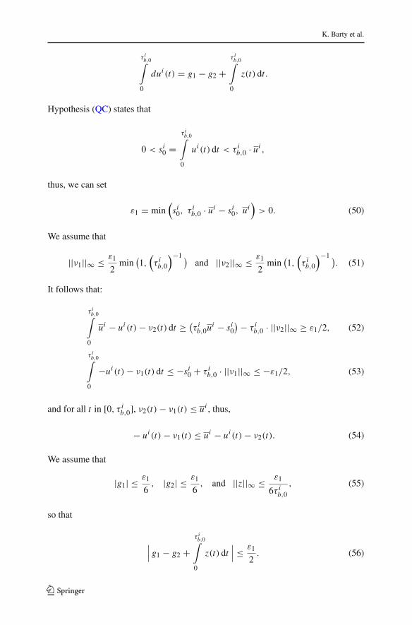
z(t) dt.

Hypothesis (QC) states that

0 < si0 =

τ ib,0∫

0

ui (t) dt < τ ib,0 · ui ,

thus, we can set

ε1 = min(

si0, τ i

b,0 · ui − si0, ui

)> 0. (50)

We assume that

||ν1||∞ ≤ ε1

2min

(1,(τ i

b,0

)−1 )and ||ν2||∞ ≤ ε1

2min

(1,(τ i

b,0

)−1 ). (51)

It follows that:

τ ib,0∫

0

ui − ui (t) − ν2(t) dt ≥ (τ i

b,0ui − si0

) − τ ib,0 · ||ν2||∞ ≥ ε1/2, (52)

τ ib,0∫

0

−ui (t) − ν1(t) dt ≤ −si0 + τ i

b,0 · ||ν1||∞ ≤ −ε1/2, (53)

and for all t in [0, τ ib,0], ν2(t) − ν1(t) ≤ ui , thus,

− ui (t) − ν1(t) ≤ ui − ui (t) − ν2(t). (54)

We assume that

|g1| ≤ ε1

6, |g2| ≤ ε1

6, and ||z||∞ ≤ ε1

6τ ib,0

, (55)

so that

∣∣∣ g1 − g2 +

τ ib,0∫

0

z(t) dt∣∣∣ ≤ ε1

2. (56)

123


Let us set

λ =

(g1 − g2 + ∫ τ i

b,00 z(t) dt

)−(∫ τ i

b,00 −ui (t) − ν1(t) dt

)

∫ τ ib,0

0 ui − ν2(t) dt − ∫ τ ib,0

0 −ν1(t) dt, (57)

we obtain, combining (52), (53), and (56) that 0 ≤ λ ≤ 1. Using (54) and (57), weobtain that the control dui defined on [0, τ i

b,0] by

dui (t) = λ[ − ν1(t) − ui (t)

] + (1 − λ)[ui − ui (t) − ν2(t)

](58)

is feasible and that the associated state dsi (t) satisfies the first state constraint.Let us focus on the construction of dui on [τ i

b,0, T ]. The final-state constraint on

dsi (T ) is satisfied if and only if

T∫

τ ib,0

dui (t) ≤ g2 − g3 + si (T ) +T∫

τ ib,0

z(t) dt.

Hypothesis (QC) states that

0 <

τ ie,0∫

τ ib,0

ai (t) dt.

We set

ε2 = min

⎛

⎜⎜⎝

τ ie,0∫

τ ib,0

ai (t) dt, ui

⎞

⎟⎟⎠ > 0. (59)

We assume now that

||ν1||∞ ≤ ε2

2min

(1,(

T − τ ib,0

)−1)

and ||ν2||∞ ≤ ε2

2. (60)

It follows that:

T∫

τ ib,0

−ui (t) − ν1(t) dt = −τ i

e,0∫

τ ib,0

ai (t) dt −T∫

τ ib,0

ν1(t) dt + si (T )

≤ −ε2 +(

T − τ ib,0

)||ν1||∞ + si (T )

≤ −ε2

2+ si (T ) (61)

123

K. Barty et al.

and for all t in [0, τ ib,0], ν2(t) − ν1(t) ≤ ui , thus

−ui (t) − ν1(t) ≤ ui − ui (t) − ν2(t).

Now, we assume that

|g2| ≤ ε2

6, |g3| ≤ ε2

6, ||z||∞ ≤ ε2

6(

T − τ ib,0

) ,

so that

g2 − g3 +T∫

τ ib,0

z(t) dt ≥ −ε2

2.

Now, we can set, for all t in [τ ib,0, T ],

dui (t) = −ui (t) − ν1(t),

It follows from (61) that:

dui (T ) ≤ −ε2/2 + si (T )

≤ g2 − g3 +T∫

τ ib,0

z(t) dt + si (T ).

As a consequence, the second state constraint is satisfied. The Lemma is proved bytaking for the constant ε a positive real number satisfying (50), (51), (55), (59), and(60). �

4.3 On convergence of solutions to the perturbed problems

The goal of this part is to check the third hypothesis of Theorem 1 for our applicationproblem. To that purpose, we fix a reference date (τb,0, τe,0) and a sequence (τb,k, τe,k)

of dates converging to (τb,0, τe,0). We suppose that hypothesis (H) holds for the ref-erence problem. Thus, it holds for k sufficiently large and there exists a sequence ofoptimal solutions (uk, sk)k to the perturbed problems (for k sufficiently large). Wedenote by (pk)k a sequence of associated costates.

In Lemma 10, we obtain the existence of a subsequence of (uk, sk)k such that(uk)k converges to an optimal control of the reference problem, u, for the weak-∗topology, and such that (sk)k converges uniformly to the associated trajectory s. InLemma 12, we prove the existence of a subsequence such that (pk)k converges to a

123


costate associated with (u, s) and, in Lemma 13, we prove that the sum of the controlsconverges uniformly. Finally, we prove the last hypothesis of Theorem 1.

Note that all the subsequences have the same name as the original sequence, forthe sake of simplicity.

Lemma 10 There exists a subsequence of (uk, sk)k such that

uk∗⇀ u in L∞(0, T ; R

n),

sk → s in L∞(0, T ; Rn),

where (u, s) is a solution to P ′(τb,0, τe,0).

Proof In this proof we first show the existence of a feasible limit point (u, s) to thesequence (uk, sk)k . Then, for any feasible trajectory (u, s) of the reference problem,we show the existence of a sequence (uk, sk)k such that both (uk)k and (sk)k convergesuniformly to (u, s) and such that for k sufficiently large, (uk, sk) is a feasible trajectoryfor the perturbed problem.

For all k, for all i in S and for all t in [0, T ],

|sik(t)| ≤ ui + ||a||∞,

|sik(t)| ≤ |si

0| + T (ui + ||a||∞),

and

||uik ||∞ ≤ ui .

Using the Arzelà–Ascoli theorem and the Banach–Alaoglu theorem, we obtain theexistence of a subsequence, still denoted by (uk, sk)k such that sk converges uniformlyto some s in L∞(0, T ; R

n), with si (0) = si0, si (τ i

b,0) = 0 and si (T ) ≥ 0 and suchthat uk converges to some u for the weak-∗ topology of L∞(0, T ; R

n). Necessarily,for almost all t in [0, T ], 0 ≤ ui (t) ≤ ui and, for all k and for all t ′,

sik(t

′) = si0 +

t ′∫

0

θk(t)(−ui

k(t) + ai ◦ θk(t)1[τ ib,0,τ

ie,0](t)

)dt

= si0 +

t ′∫

0

−(θk(t) − 1

)ui

k(t) dt

+t ′∫

0

(θk(t) − 1

)ai ◦ θk(t)1[τ i

b,0,τie,0](t) dt

123

K. Barty et al.

+t ′∫

0

−(

uik(t) − ui (t)

)dt +

t ′∫

0

(ai ◦ θk(t) − ai (t)

)1[

τ ib,0,τ i

e,0

](t) dt

+t ′∫

0

−ui (t) + ai (t)1[τ i

b,0,τ ie,0

](t) dt. (62)

Using (45), (46), and the weak-∗ convergence of (uk)k , we obtain, to the limit,

si (t) = si0 +

t ′∫

0

−ui (t) + ai (t)1[τ ib,0,τ i

e,0](t) dt,

which proves that s satisfies the differential equation of the reference problem, hence(u, s) is feasible.

Let (u, s) be a feasible control of the reference problem. It can be proved (with thesame kind of estimates as in (62) that

si0 +

τ ib,0∫

0

θk(t)

(−ui (t) + ai ◦ θk(t)1[

τ ib,0,τ i

e,0

](t)

)dt = s

(τ i

b,0

)+ o(1) = o(1),

si0 +

T∫

0

θk(t)

(−ui (t) + ai ◦ θk(t)1[

τ ib,0,τ i

e,0

](t)

)dt = s(T ) + o(1) = o(1),

Since Robinson’s qualification holds for the trajectory (u, s) by Lemma 9, we obtain,using the stability theorem [1, theorem 2.87] that there exists a sequence of feasibletrajectories (uk, sk) for the perturbed problems such that (uk)k and (sk)k convergesuniformly to u and s respectively.

Finally, we have that

T∫

0

�(t, uk(t)

)dt ≤

T∫

0

�(t, uk(t)

)dt,

thus passing to the lim inf in the left-hand-side (like in 48) and passing to the limit inthe right-hand-side, we obtain that

T∫

0

�(t, u(t)

)dt ≤

T∫

0

�(t, u(t)

)dt,

which proves the optimality of (u, s). The Lemma follows. �

123


Lemma 11 The sequence (pk) is bounded.

Proof This result derives from the study of �(τb,0, τe,0) conducted in Theorem 3. Thequalification condition (QC) being stable, it is satisfied for k sufficiently large. Whenthe qualification condition is satisfied, it is impossible that ui (t) = 0 for almost all tin [0, τ i

b,0] or that ui (t) = ui for almost all t in [0, τ ib,0], thus the associated bounds

πi,min0 and π

i,max0 are finite. More precisely, denoting respectively by dmin and dmax

the infimum and the supremum of d over [0, T ], we obtain that

−c′(dmax) ≤ pik(0) ≤ −c′(dmin −

∑

i∈S

ui),

since −c′ is non-increasing. This proves the boundedness of pk(0). For the studyof pk(T ), let us recall first that up to a subsequence, a sequence (uk, sk) of optimalsolutions to the perturbed problems is such that sk(T ) converges. Let BT a compactof R

n be such that sk(T ) belongs to BT for k big enough. There are two cases: ifsi

k(T ) > 0, then

infs∈BT

Dsi φ(s) ≤ Dsi φ(sk(T )) = pik(T ) ≤ sup

s∈BT

Dsi φ(s)

otherwise, sik(T ) = 0 and by qualification, it is impossible to have ui

k(t) = 0 for all tin [τ i

e,0, T ] in this case, thus

−c′(dmax) ≤ pik(T ) ≤ sup

s∈BT

Dsi φ(s).

Finally, we obtain that

min{

− c′(dmax), infs∈BT

Dsi φ(s)}

≤ pik(T ) ≤ sup

s∈BT

Dsi φ(s),

whence the boundedness of (pk)k . �Lemma 12 Up to a subsequence, (pk)k converges to some p in �(τb,0, τe,0).

Proof Recall that p is viewed as an element of R2n , therefore we do not need to be

precise about the topology involved for the convergence. By Lemma 10, we can extract

from this sequence a sequence of solutions, denoted by (uk, sk) such that uk∗⇀ u and

sk → s (in L∞(0, T ; Rn)) where (u, s) is a solution to P(τb,0, τe,0).

By Lemma 11, the sequences pk(0) and pk(T ) are bounded, and thus we can extracta subsequence such that these sequences converge to say p0 and pT . Let us prove thatp = (p0, pT ) belongs to �(τb,0, τe,0). Recall that the Hamiltonian associated theperturbed problem is

θk(t)HW (t)(θk(t), u, p

).

123

K. Barty et al.

Let a and b be such that 0 ≤ a < b ≤ T , let v in L∞(0, T ) be such that for almost all tin [0, T ], for all i in S, 0 ≤ vi (t) ≤ ui . In order to show that p belongs to �(τb,0, τe,0),it suffices to show that:

b∫

a

HW (t)(t, p(t), u(t)) dt ≤b∫

a

HW (t)(t, p(t), v(t)) dt.

Applying Pontryagin’s principle to the perturbed problem, we obtain directly that

b∫

a

HW (t)(θk(t), uk(t), pk(t)

)dt ≤

b∫

a

HW (t)(θk(t), v(t), pk(t)

)dt. (63)

Let us focus on the integral of the left-hand-side. We have

b∫

a


)dt

=b∫

a


) − HW (t)(t, uk(t), pk(t)

)dt

+b∫

a

HW (t)(t, uk(t), pk(t)

) − HW (t)(t, uk(t), p(t)

)dt

+b∫

a

HW (t)(t, uk(t), p(t)

) − HW (t)(t, u(t), p(t)

)dt

+b∫

a


)dt.

Using (45), (46), the uniform convergence of (pk)k , the weak-∗ lower semi-continuityof the integral of the Hamiltonian (see 48 for the idea of a proof), we obtain that tothe limit,

lim infk→∞

b∫

a

θ ′k(t)HW (t)

(θk(t), uk(t), pk(t)

)dt ≤

b∫

a


)dt.

123


Similarly, we can show that

limk→∞

b∫

a

θ ′k(t)HW (t)

(θk(t), v(t), pk(t)

)dt =

b∫

a

HW (t)(t, v(t), p(t)

)dt.

Thus, passing to the limit in (63), we obtain

b∫

a


)dt ≤

b∫

a

HW (t)(t, v(t), p(t)

)dt,

which proves that p belongs to �(τb,0, τe,0), hence the Lemma. �

Lemma 13 Up to a subsequence,

∑

i∈S

uik −→

∑

i∈S

ui in L∞(0, T ; Rn).

Proof As usual, we set μk(t) = ∑i∈S

uik(t). Let us set

HW : R × Rn × R

n → R(d, μ, p) �→ c(d(t) − μ) + ξW (μ, p),

where W is a given subset of S. This function looks like a Hamiltonian, however,notice that the demand is viewed as a parameter now. Moreover, the part involving therefuelling a(t) is missing. For almost all t in [0, T ],

μk(t) = minμ∈[0,

∑i∈W (t) ui ]

HW (t)

(d ◦ θk(t), μ, pk(t)

). (64)

Thanks to the reparameterization, when t is given, μk(t) minimizes a function HW (t)

independent on k. Recall that the cost function c is α-convex and so is the functionμ �→ HW (d, p, μ). Considering that the optimization problem given by (64) is aproblem parameterized by d◦ θk and pk , we obtain by a classical property of stability ofoptimal solutions (see [1, proposition 4.32]) that there exists a constant A independenton time such that for almost all t in [0, T ],

|μk(t) − μ(t)| ≤ A(|pk(t) − p(t)| + |d ◦ θk(t) − d(t)|), (65)

By Lemma 12, we know that up to a subsequence, (pk(0), pk(T )) converges to somep in �(τb, τe). Since the times of discontinuity of p are fixed, this implies the uniformconvergence of the costate, when considered as a time function. Moreover, it is easy tocheck that the sequence (d◦ θk(t))k converges uniformly to d(t), since d(t) is Lipschitz

123

K. Barty et al.

and since (θk)k converges uniformly to the identity function on [0, T ]. Together with(65), we obtain that

||μk − μ||∞ ≤ A(||pk − p||∞ + ||d ◦ θk − d||∞

) → 0.

as was to be proved. �Lemma 14 If hypotheses (H) and (QC) hold, then hypothesis 3 of Theorem 1 issatisfied for any direction of perturbation.

Proof We know by lemmas 10 and 13 that up to a subsequence, for all i in S,

uik

∗⇀ ui and μk =

∑

i∈S

uik → μ =

∑

i∈S

ui .

Consider a sequence of times (τb,k, τe,k) such that for all k,

(τb,k, τe,k) ∈ [(τb,0, τe,0), (τb,k, τe,k)].

For simplicity, we consider that the direction of perturbation is a unit basic vector indirection τ

je , so that we can refer to expression (28) for the derivative of the Lagrangian,

and we use the same notations. We have:

Dτ

jeL(uk, s, p, (τb,k, τe,k)

)

=[ 1

τ0 − t1

τ0∫

t1

HW (θτb,k ,τe,k (t), uk(t), p) dt

+ τj

e,k − t1

τ0 − t1

τ0∫

t1

t − t1τ0 − t1

Dt HW (θτb,k ,τe,k (t), uk(t), p) dt]

−[ 1

t2 − τ0

t2∫

τ0

HW∪{ j}(θτb,k ,τe,k (t), uk(t), p) dt

− t2 − τj

e,k

t2 − τ0

t2∫

τ0

t2 − t

t2 − τ0Dt HW∪{ j}(θτb,k ,τe,k (t), uk(t), p) dt

].

Moreover, for all t in [t1, τ0],

HW (θτb,k ,τe,k (t), uk(t), p)

= c(

d ◦ θτb,k ,τe,k (t) −∑

i∈W

uk(t))

+∑

i∈S

pi ( − ui (t) + ai ◦ θτb,k ,τe,k (t)1i /∈W),

123


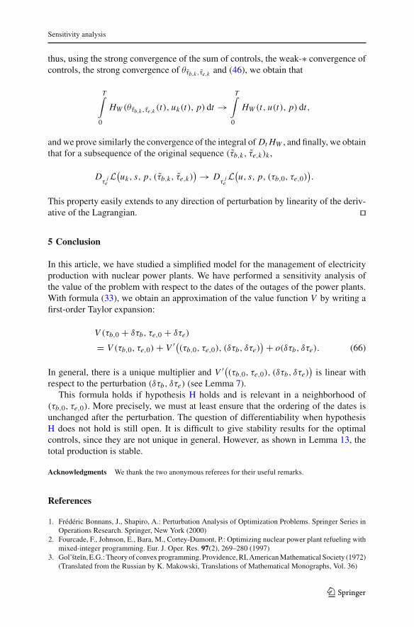
thus, using the strong convergence of the sum of controls, the weak-∗ convergence ofcontrols, the strong convergence of θτb,k ,τe,k and (46), we obtain that

T∫

0

HW (θτb,k ,τe,k (t), uk(t), p) dt →T∫

0

HW (t, u(t), p) dt,

and we prove similarly the convergence of the integral of Dt HW , and finally, we obtainthat for a subsequence of the original sequence (τb,k, τe,k)k ,

Dτ

jeL(uk, s, p, (τb,k, τe,k)

) → Dτ

jeL(u, s, p, (τb,0, τe,0)

).

This property easily extends to any direction of perturbation by linearity of the deriv-ative of the Lagrangian. �

5 Conclusion

In this article, we have studied a simplified model for the management of electricityproduction with nuclear power plants. We have performed a sensitivity analysis ofthe value of the problem with respect to the dates of the outages of the power plants.With formula (33), we obtain an approximation of the value function V by writing afirst-order Taylor expansion:

V (τb,0 + δτb, τe,0 + δτe)

= V (τb,0, τe,0) + V ′((τb,0, τe,0), (δτb, δτe)) + o(δτb, δτe). (66)

In general, there is a unique multiplier and V ′((τb,0, τe,0), (δτb, δτe))

is linear withrespect to the perturbation (δτb, δτe) (see Lemma 7).

This formula holds if hypothesis H holds and is relevant in a neighborhood of(τb,0, τe,0). More precisely, we must at least ensure that the ordering of the dates isunchanged after the perturbation. The question of differentiability when hypothesisH does not hold is still open. It is difficult to give stability results for the optimalcontrols, since they are not unique in general. However, as shown in Lemma 13, thetotal production is stable.

Acknowledgments We thank the two anonymous referees for their useful remarks.

References

1. Frédéric Bonnans, J., Shapiro, A.: Perturbation Analysis of Optimization Problems. Springer Series inOperations Research. Springer, New York (2000)

2. Fourcade, F., Johnson, E., Bara, M., Cortey-Dumont, P.: Optimizing nuclear power plant refueling withmixed-integer programming. Eur. J. Oper. Res. 97(2), 269–280 (1997)

3. Gol’šteın, E.G.: Theory of convex programming. Providence, RI, American Mathematical Society (1972)(Translated from the Russian by K. Makowski, Translations of Mathematical Monographs, Vol. 36)

123

K. Barty et al.

4. Ioffe, A.D., Tihomirov, V.M.: Theory of Extremal Problems, Volume 6 of Studies in Mathematics andits Applications. North-Holland Publishing Co., Amsterdam (1979) (Translated from the Russian byKarol Makowski)

5. Khemmoudj, M., Porcheron, M., Bennaceur, H.: When constraint programming and local search solvethe scheduling problem of Electricité de France nuclear power plant outages. In: Benhamou, F. (ed.)Principles and Practice of Constraint Programming–CP 2006, Lecture Notes in Computer Science, vol.4204, pp. 271–283. Springer, Berlin (2006)

6. Khemmoudj, M.O.I.: Modélisation et résolution de systèmes de contraintes: Application au problèmede placement des arrêts et de la production des réacteurs nucléaires d’ EDF. PhD Thesis, April (2007)

7. Porcheron, M., Gorge, A., Juan, O., Simovic, T., Dereu, G.: Challenge ROADEF/ EURO 2010: Alarge-scale energy management problem with varied constraints. http://challenge.roadef.org/2010/files/sujetEDFv22.pdf. February (2010)

123

http://challenge.roadef.org/2010/files/sujetEDFv22.pdf

http://challenge.roadef.org/2010/files/sujetEDFv22.pdf

Documents

Sensitivity analysis for the outages of nuclear power plants