SENSITIVITY ANALYSIS OF STREETER-PHELPS MODELS S. RINALDI~AND R. SONCINI-SESSA* FEBRUARY 1977

* Centro Teoria dei Sistemi. C.N.R.. Via Ponzio. 3415, Milano, Italy.

This work was supported jointly by IIASA and the Centro Teoria dei Sistemi. C.N.R., Via Ponzio. 3415. Milano, Italy.

Research Reports provide the formal record of research conducted by the International Institute for Applied Systems Analysis. They are carefully reviewed before publication and represent, in the Institute's best judgment, competent scientific work. Views or opinions expressed herein, however, do not necessarily reflect those of the National Member Organizations support- ing the Institute or of the Institute itself.

International lnstitute for Applied Systems Analysis 2361 Laxenburg, Austria

PREFACE

This report is one of a series describing IIASA research into approaches for comparing alternative models that could be applied to the establishment of control policies to meet water-quality standards. In addition to model evaluation, this project has focused on prob- lems of optimization and conflict resolution in large river basins.

ABSTRACT

Sensitivity theory is applied in this paper to a class of generalized Streeter-Phelps models in order to predict the variations induced in BOD by the variations of some para- meters characterizing the river system.

The paper shows how simple and elegant this technique is. and at the same time proves that many relatively complex phenomena can be explained by Streeter-Phelps models.

Sensitivity Analysis of Streeter-Phelps Models

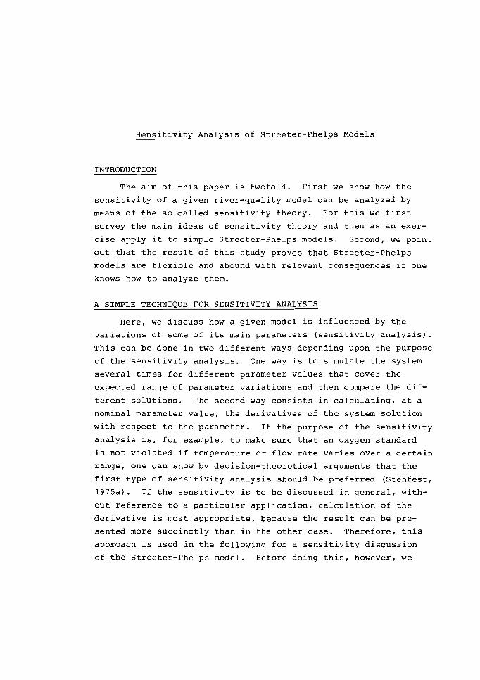
INTRODUCTION

The aim of this paper is twofold. First we show how the

sensitivity of a given river-quality model can be analyzed by

means of the so-called sensitivity theory. For this we first

survey the main ideas of sensitivity theory and then as an exer-

cise apply it to simple Streeter-Phelps models. Second, we point

out that the result of this study proves that Streeter-Phelps

models are flexible and abound with relevant consequences if one

knows how to analyze them.

A SIMPLE TECHNIQUE FOR SENSITIVITY ANALYSIS

Here, we discuss how a given model is influenced by the

variations of some of its main parameters (sensitivity analysis).

This can be done in two different ways depending upon the purpose

of the sensitivity analysis. One way is to simulate the system

several times for different parameter values that cover the

expected range of parameter variations and then compare the dif-

ferent solutions. The second way consists in calculating, at a

nominal parameter value, the derivatives of the system solution

with respect to the parameter. If the purpose of the sensitivity

analysis is, for example, to make sure that an oxygen standard

is not violated if temperature or flow rate varies over a certain

range, one can show by decision-theoretical arguments that the

first type of sensitivity analysis should be preferred (Stehfest,

1975a). If the sensitivity is to be discussed in general, with-

out reference to a particular application, calculation of the

derivative is most appropriate, because the result can be pre-

sented more succinctly than in the other case. Therefore, this

approach is used in the following for a sensitivity discussion

of the Streeter-Phelps model. Before doing this, however, we

b r i e f l y p r e s e n t t h e e l e m e n t s o f t h i s t y p e o f s e n s i t i v i t y a n a l y -

s i s ( s e e , f o r example, Cruz, 1 9 7 3 ) .

Assume t h a t a c o n t i n u o u s , lumped p a r a m e t e r sys tem i s de-

s c r i b e d by t h e v e c t o r d i f f e r e n t i a l e q u a t i o n

where x i s a n n - th o r d e r v e c t o r and 8 i s a c o n s t a n t p a r a m e t e r

w i t h nominal v a l u e 8 , and l e t t h e i n i t i a l s t a t e xo o f t h e s y s -

t e m depend upon t h e p a r a m e t e r , i . e .

The s o l u t i o n o f Eq. (1) w i t h t h e i n i t i a l c o n d i t i o n ( 2 ) i s a

f u n c t i o n

which, under v e r y g e n e r a l c o n d i t i o n s , c a n be expanded i n s e r i e s

i n t h e neighborhood o f t h e nominal v a l u e o f t h e p a r a m e t e r , i . e .

where x ( t ) = x ( t , 8 ) i s t h e nominal s o l u t i o n . The v e c t o r

[ax/aOlg , namely t h e d e r i v a t i v e o f t h e s t a t e v e c t o r w i t h r e s p e c t

t o t h e p a r a m e t e r , i s c a l l e d t h e s e n s i t i v i t y v e c t o r ( o r s e n s i t i v -

i t y c o e f f i c i e n t ) and f rom now on w i l l b e deno ted by s , i . e .

Thus the perturbed solution of Eq. (1) can be easily obtained as

once the sensitivity vector is known.

When there are many parameters 81,82,...,8q, the knowledge

of the sensitivity vectors s 1,~2r...r~q allows the association

of specific characteristics of the system behavior with particu-

lar parameters. If, for example, the nominal solution x(t) of

a first-order system is the one shown in Figure 1, where sl(t)

and s2 (t) are the sensitivity coefficients of x with respect to

two parameters €I1 and €I2, one can say that the first parameter

is responsible for the overshoot of x while the second is responsible for the asymptotic behavior of the system. This

characterization of the parameters very often turns out to be

of great importance in the validation of the structure of a

model; in fact some of the best-known methods of parameter

estimation are based on manipulation of the sensitivity vectors.

Figure 1. Nominal solution ii and sensitivity coefficients s l and sg.

By t a k i n g t h e t o t a l d e r i v a t i v e of Eq. (1) it can be con-

c luded t h a t t h e s e n s i t i v i t y v e c t o r s ( t ) s a t i s f i e s t h e fo l lowing

v e c t o r d i f f e r e n t i a l equat ion:

wi th i n i t i a l cond i t i ons

Thus, t h e s e n s i t i v i t y vec to r i s t h e s t a t e vec to r of t h e system (31,

c a l l e d s e n s i t i v i t y system, which i s always a l i n e a r system, even

i f system (1) is non l inea r . Because of t h i s p rope r ty t h e s e n s i -

t i v i t y v e c t o r s can o f t e n be a n a l y t i c a l l y determined. I n any c a s e ,

t hey can always be computed by means of s imu la t ion fo l lowing t h e

scheme shown i n F igu re 2 .

Figure 2. Computation of sensitivity vectors.

. SENSITIVITY SYSTEM 1

, Si b

NOMINAL SYSTEM

- x

4 )

, SYSTEM M

b SENSITIVITY S~

I n t h e f o l l o w i n g we a p p l y t h i s methodology t o some v e r y

p a r t i c u l a r b u t i n t e r e s t i n g s e n s i t i v i t y problems of r i v e r p o l l u t i o n .

The model we u s e i s t h e well-known S t r e e t e r - P h e l p s model o r some

s u i t a b l e m o d i f i c a t i o n o f it. To s i m p l i f y t h e d i s c u s s i o n we d e a l

w i t h t h e p a r a m e t e r s o n e a t a t i m e . Obvious ly , t h i s d o e s n o t imply

t h a t o u r r e s u l t s a r e n o t g e n e r a l , s i n c e i n t h e c a s e of many para -

meters 81 ,82 , . . . t h e p e r t u r b e d s o l u t i o n o f E q . (1) can b e s imply

o b t a i n e d a s

where s l ( t ) , s 2 ( t ) , ... a r e t h e s e n s i t i v i t y v e c t o r s .

BOD VARIATIONS

L e t u s f i r s t a n a l y z e t h e e f f e c t s o f a v a r i a t i o n o f t h e BOD

l o a d d i s c h a r g e d i n t o t h e r i v e r a t a p a r t i c u l a r p o i n t . By w r i t i n g

t h e S t r e e t e r - P h e l p s model i n f low t i m e T we o b t a i n t h a t t h e s y s -

tem i s d e s c r i b e d by

where b and c s t a n d f o r BOD and DO, cs i s t h e oxygen s a t u r a t i o n

l e v e l and kl and k2 a r e t h e c h a r a c t e r i s t i c p a r a m e t e r s (BOD decay

and r e - a e r a t i o n c o e f f i c i e n t s , r e s p e c t i v e l y ) o f t h e model. The

i n i t i a l c o n d i t i o n s a r e

i f we assume t h a t t h e oxygen c o n t e n t o f t h e e f f l u e n t i s n e g l i g i -

b l e . Thus, t h e s e n s i t i v i t y sys tem i s g i v e n by

and i t s i n i t i a l c o n d i t i o n s a r e

The s o l u t i o n o f Eq. ( 5 a ) w i t h sb = 1 i s g i v e n by 0

which can b e i n t r o d u c e d i n Eq. (5b) t o g e t h e r w i t h s = 0, t h u s

g i v i n g 0

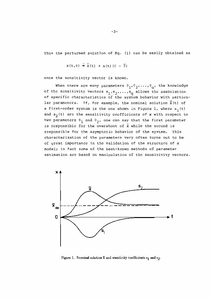
The s e n s i t i v i t y c o e f f i c i e n t s g i v e n by Eq. ( 6 ) i s always nega- C

t i v e , a s shown i n F i g u r e 3 , and h a s a minimum f o r

T h i s means t h a t a p o s i t i v e p e r t u r b a t i o n o f t h e BOD l o a d a t a

p o i n t on t h e r i v e r i m p l i e s t h a t a l l t h e r i v e r downstream from

Figure 3. The sensitivity of dissolved oxygen concentration to ROD load.

t h a t p o i n t becomes worse a s f a r a s i t s oxygen c o n t e n t i s con-

c e r n e d . T h i s i s t h e c o n c l u s i o n o n e can d e r i v e from t h e S t r e e t e r -

P h e l p s model which d o e s n o t r e p r e s e n t a p r i o r i t h e b e h a v i o r of a

r e a l r i v e r . Indeed , it can b e shown ( s e e , f o r i n s t a n c e , S t e h f e s t ,

1975b) t h a t b e c a u s e of t h e mechanisms o f t h e food c h a i n , i t c o u l d

sometimes b e e x p e c t e d t h a t t h e c o n d i t i o n s o f t h e r i v e r a r e b e t -

t e r e d a t some p a r t i c u l a r p o i n t by an i n c r e a s e o f t h e BOD l o a d .

FLOW VARIATIONS

L e t u s now suppose t h a t we a r e i n t e r e s t e d i n p r e d i c t i n g t h e

v a r i a t i o n s induced i n BOD and DO i n a s t r e a m by v a r i a t i o n s o f

f low r a t e ( s e e , f o r example, Loucks and Jacoby , 1 9 7 2 ) . Of c o u r s e

w e c a n n o t c o n s i d e r f low t i m e a s t h e independent v a r i a b l e and we

must t h e r e f o r e w r i t e t h e S t r e e t e r - P h e l p s model i n t h e form

where L i s d i s t a n c e , Q i s f l o w r a t e and t h e two new c h a r a c t e r i s -

t i c p a r a m e t e r s a r e g i v e n by

v(Q) b e i n g t h e a v e r a g e s t r e a m v e l o c i t y .

A s f a r a s t h e i n i t i a l c o n d i t i o n s a r e concerned , l e t u s sup-

pose t h a t t h e w a t e r coming i n t o t h e r e a c h u n d e r c o n s i d e r a t i o n i s

p e r f e c t l y oxygenated and w i t h z e r o BOD. Thus, a f t e r mixing w i t h

t h e e f f l u e n t d i s c h a r g e i n p o i n t L = 0 we have

s o t h a t t h e i n i t i a l c o n d i t i o n s o f t h e s e n s i t i v i t y v e c t o r t u r n o u t

t o be g i v e n by

w h i l e t h e s e n s i t i v i t y sys tem ( 3 ) is g i v e n by

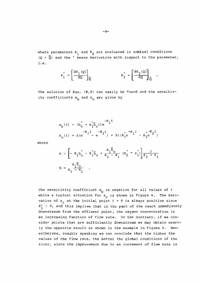
where parameters K1 and K2 are evaluated in nominal conditions

(Q = 5 ) and the ' means derivative with respect to the parameter, i.e.

The solution of Eqs. (8,9) can easily be found and the sensitiv-

ity coefficients sb and sc are given by

where

The sensitivity coefficient sb is negative for all values of .L

while a typical situation for sc is shown in Figure 4. The deri-

vative of sc at the initial point & = 0 is always positive since

Ki < 0, and this implies that in the part of the reach immediately

downstream from the effluent point, the oxygen concentration is

an increasing function of flow rate. On the contrary, if we con-

sider points that are sufficiently downstream we may obtain exact-

ly the opposite result as shown in the example in Figure 4. Nev-

ertheless, roughly speaking we can conclude that the higher the

values of the flow rate, the better the global conditions of the

river, since the improvement due to an increment of flow rate is

o b t a i n e d where t h e oxygen c o n d i t i o n s a r e worse ; t h i s f a c t i s

a c t u a l l y t h e m o t i v a t i o n f o r t h e u s e o f low-flow augmenta t ion

( s e e Loucks and Jacoby , 1972) i n r i v e r - q u a l i t y c o n t r o l .

Figure 4. 'The sensitivity of dissolved oxygen concentration to flow rate.

TEMPERATURE VARIATIONS

L e t u s now d i s c u s s t h e i n f l u e n c e o f t h e t e m p e r a t u r e on t h e

d i s s o l v e d oxygen o f a r i v e r . To s i m p l i f y t h e d i s c u s s i o n l e t u s

assume we a r e d i s c h a r g i n g a g i v e n amount o f BOD a t a p a r t i c u l a r

p o i n t o f a p e r f e c t l y c l e a n and oxygena ted r i v e r . Moreover, sup-

p o s e t h a t t h e s t e a d y - s t a t e ( e q u i l i b r i u m ) t e m p e r a t u r e T o f t h e

w a t e r i s c o n s t a n t i n s p a c e . Thus, t h e i n i t i a l c o n d i t i o n s o f t h e

s t r e t c h a r e g i v e n and depend upon t h e t e m p e r a t u r e T o f t h e w a t e r

s i n c e t h e oxygen s a t u r a t i o n l e v e l c i s a d e c r e a s i n g f u n c t i o n o f s T. Under t h e s e a s s u m p t i o n s t h e sys tem i s d e s c r i b e d by

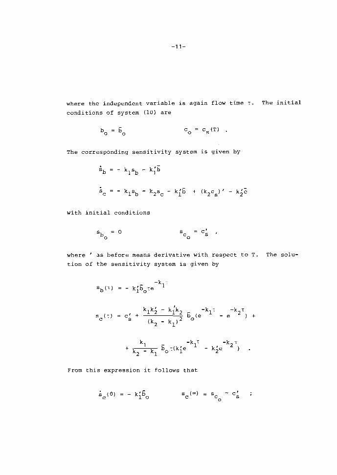
where the independent variable is again flow time T . The initial

conditions of system (10) are

The corresponding sensitivity system is given by

- Sb = - klSb - k;b

with initial conditions

where ' as before means derivative with respect to T. The solu-

tion of the sensitivity system is given by

From this expression it follows that

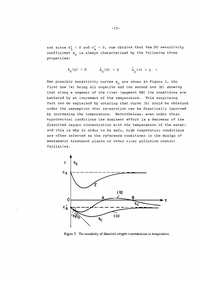
and since ki < 0 and c& < 0, one obtains that the DO sensitivity

coefficient s is always characterized by the following three C

properties:

Two possible sensitivity curves s are shown in Figure 5, the C

first one (a) being all negative and the second one (b) showing

that along a segment of the river (segment AB) the conditions are

bettered by an increment of the temperature. This surprising

fact can be explained by noticing that curve (b) could be obtained

under the assumption that re-aeration can be drastically improved

by increasing the temperature. Nevertheless, even under these

hypothetical conditions the dominant effect is a decrease of the

dissolved oxygen concentration with the temperature of the water;

and this is why in order to be safe, high temperature conditions

are often selected as the reference conditions in the design of

wastewater treatment plants or other river pollution control

facilities.

Figure 5. The sensitivity of dissolved oxygen concentration to temperature.

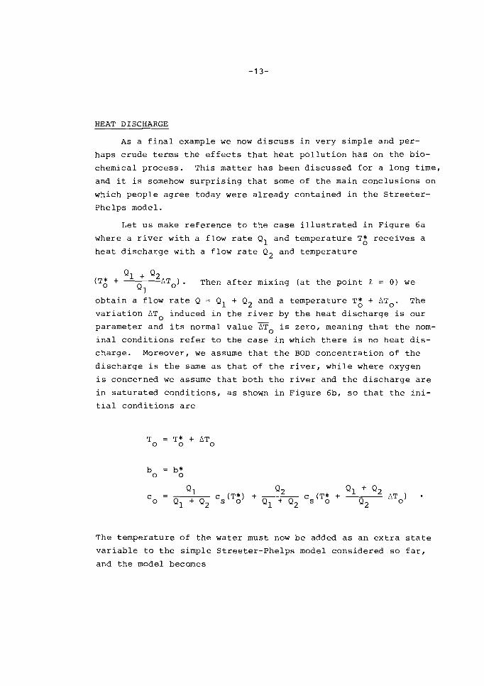
HEAT DISCHARGE

As a f i n a l example we now d i s c u s s i n ve ry s imple and per -

haps c rude te rms t h e e f f e c t s t h a t h e a t p o l l u t i o n ha s on t h e b io-

chemica l p roce s s . Th i s m a t t e r ha s been d i s c u s s e d f o r a long t i m e ,

and it i s somehow s u r p r i s i n g t h a t some of t h e main c o n c l u s i o n s on

which peop l e a g r e e today were a l r e a d y con t a ined i n t h e S t r e e t e r -

Phe lps model.

Le t u s make r e f e r e n c e t o t h e c a s e i l l u s t r a t e d i n F i g u r e 6a

where a r i v e r w i t h a f low r a t e Q1 and t empe ra tu r e T: r e c e i v e s a

h e a t d i s c h a r g e w i t h a f l ow r a t e Q 2 and t empe ra tu r e

Ql + Q2 (T: + -- ATo). Then a f t e r mixing ( a t t h e p o i n t R = 0) we

1 o b t a i n a f low r a t e Q = Q1 + Q2 and a t empe ra tu r e T* + ATo. The

0

v a r i a t i o n ATo induced i n t h e r i v e r by t h e h e a t d i s c h a r g e i s ou r

parameter and i t s normal v a l u e is ze ro , meaning t h a t t h e nom- 0

i n a l c o n d i t i o n s r e f e r t o t h e c a s e i n which t h e r e i s no h e a t d i s -

cha rge . Moreover, we assume t h a t t h e BOD c o n c e n t r a t i o n o f t h e

d i s c h a r g e i s t h e same a s t h a t of t h e r i v e r , w h i l e where oxygen

i s concerned we assume t h a t bo th t h e r i v e r and t h e d i s c h a r g e a r e

i n s a t u r a t e d c o n d i t i o n s , a s shown i n F i g u r e 6b, s o t h a t t h e i n i -

t i a l c o n d i t i o n s a r e

The t empe ra tu r e o f t h e wa t e r must now b e added a s a n e x t r a s t a t e

v a r i a b l e t o t h e s imple S t r e e t e r - P h e l p s model cons ide r ed s o f a r ,

and t h e model becomes

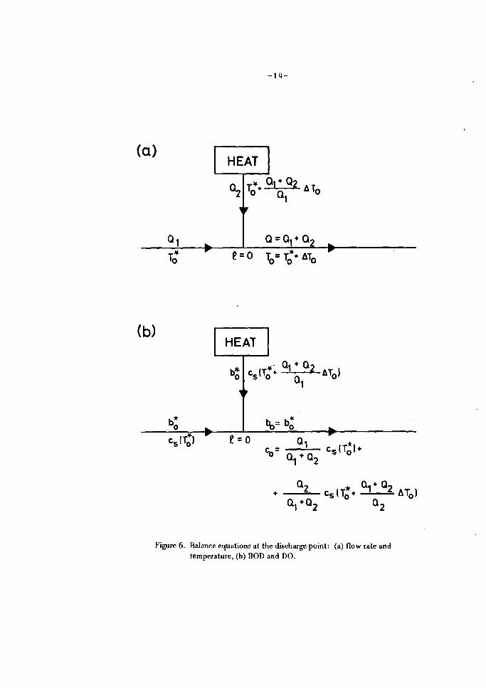
Figure 6 . Ralance equations at the discharge point: (a) flow rate and temperature, (b) BOD and DO.

.i. = f (T )

w i t h i n i t i a l n o m i n a l c o n d i t i o n s

- - - T = Tr,

0 bo = b; c = c ~ ( T * ~ ) 0

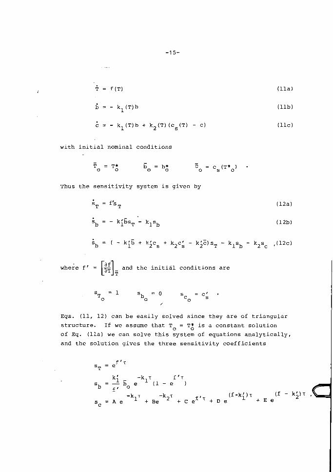
Thus t h e s e n s i t i v i t y s y s t e m i s g i v e n by

= f l s T T

= - b k i E s T - klsb

6 = ( - k i 6 + k;cs + k2c; - k;E)sT - klsb - k2sc b , ( 1 2 ~ )

w h e r e f r = i. and t h e i n i t i a l c o n d i t i o n s a r e Pf1

Eqs. (11, 1 2 ) c a n b e e a s i l y s o l v e d s i n c e t h e y a r e o f t r i a n g u l a r

s t r u c t u r e . I f we a s sume t h a t T = T; i s a c o n s t a n t s o l u t i o n 0

o f Eq. ( l l a ) we c a n s o l v e t h i s s y s t e m o f e q u a t i o n s a n a l y t i c a l l y ,

a n d t h e s o l u t i o n g i v e s t h e t h r e e s e n s i t i v i t y c o e f f i c i e n t s

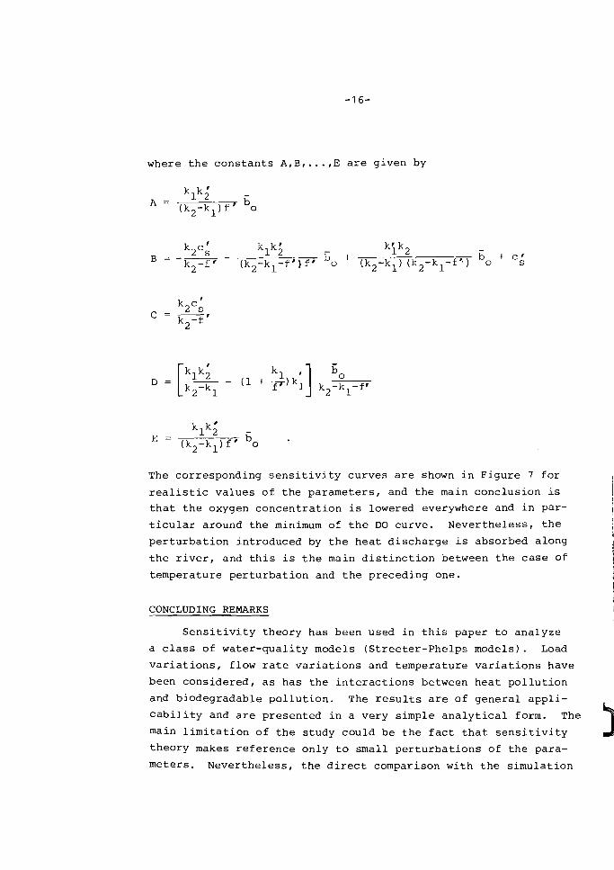
where the constants A,B,. ..,E are given by

k2ci k1k5 - B = kik2 k2-fr (k2-kl-f.) f' bo + (k2-kl) (i; -k -it,)

Go + C; 2 1

The corresponding sensitivity curves are shown in Figure 7 for

realistic values of the parameters, and the main conclusion is

that the oxygen concentration is lowered everywhere and in par-

ticular around the minimum of the DO curve. Nevertheless, the

perturbation introduced by the heat discharge is absorbed along

the river, and this is the main distinction between the case of

temperature perturbation and the preceding one.

CONCLUDING REMARKS

Sensitivity theory has been used in this paper to analyze

a class of water-quality models (Streeter-Phelps models). Load

variations, flow rate variations and temperature variations have

been considered, as has the interactions between heat pollution

and biodegradable pollution. The results are of general appli-

cability and are presented in a very simple analytical form. The

main limitation of the study could be the fact that sensitivity

theory makes reference only to small perturbations of the para-

meters. Nevertheless, the direct comparison with the simulation

Figure 7. Sensitivity coefficients of temperature, BOD and DO to heat discharge.

study carried out by Lin et al. (1973) has shown that the results

obtained in this paper are largely satisfactory for realistic

variations of the parameters of river-quality models.

REFERENCES

Cruz, J.B. (1973), S y s t e m s S e n s i t i v i t y A n a l y s i s , Dowden, Hutchinson and Ross, Strandsburg, Pennsylvania.

Lin, S.H., L.T. Fan and C.L. Hwang (1973), Digital Simulation of the Effect of Thermal Discharge on Stream Water Quality, W.R. B u l l , 9 , 4, 689-702.

Loucks, D.P. and H.D. Jacoby (19721, Flow Regulations for Water Quality Management, in Models f o r Managing R e g i o n a l Water Q u a l i t y , ed. H.A. Thomas, Harvard University Press, Cambridge, Mass.

Stehfest, H. (1975a), Decision Theoretical Remark on Sensitivity Analysis, RR-75-3, International Institute for Applied Systems Analysis, Laxenburg, Austria.

Stehfest, H. (1975b), Mathematical Modeling of Self-Purification of Rivers (in German), KFK 1654 UF, Kernforschungszentrum Karlsruhe (English translation available as internal paper of the International Institute for Applied Systems Analysis, Laxenburg, Austria).