Sensitivity of a Cloud-Resolving Simulation of the …rams.atmos.colostate.edu/cotton/vita/149.pdf934 JOURNAL OF HYDROMETEOROLOGY VOLUME 5 q 2004 American Meteorological Society Sensitivity

934 VOLUME 5J O U R N A L O F H Y D R O M E T E O R O L O G Y

q 2004 American Meteorological Society

Sensitivity of a Cloud-Resolving Simulation of the Genesis of a Mesoscale ConvectiveSystem to Horizontal Heterogeneities in Soil Moisture Initialization

WILLIAM Y. Y. CHENG AND WILLIAM R. COTTON

Department of Atmospheric Science, Colorado State University, Fort Collins, Colorado

(Manuscript received 18 August 2002, in final form 17 March 2004)

ABSTRACT

This study examines the sensitivity of varying the horizontal heterogeneities of the soil moisture initialization(SMI) in the cloud-resolving grid of a real-data simulation of a midlatitude mesoscale convective system (MCS)during its genesis phase. The quasi-stationary MCS of this study formed in the Texas/Oklahoma panhandle witha lifetime of 9 h (2200 UTC 26 July to 0700 UTC 27 July 1998). Soil moisture for the finest nested grid (thecloud-resolving grid) was derived from the antecedent precipitation index (API) using 4-km-grid-spacing pre-cipitation data for a 3-month period. In order to vary the heterogeneities of the SMI in the cloud-resolving grid,(i) Barnes objective analysis was used to alter the resolution of the soil moisture initialization, (ii) the amplitudesof the soil moisture anomalies were reduced, (iii) the position of a soil moisture anomaly was altered, and (iv)two experiments with homogeneous SMI (31% and 50% saturation) were performed. Because of the severedrought in the Texas/Oklahoma panhandle area, the saturation API value was lowered in order to introduceheterogeneities in the soil moisture for the sensitivity experiments.

All of the experiments with heterogeneous SMI (in addition to an experiment with a homogeneous SMI at31% saturation) produced an MCS with a quasi-circular cloud shield, similar to the observed timing, size, andlocation. The authors’ findings suggest that a soil moisture dataset with approximately 40-km grid spacing maybe adequate to initialize a cloud-resolving model for simulating MCSs. For the simulations in this study, thesoil moisture distribution determined where convection was likely to occur. Wetter soil tended to suppressconvection for this case, and convection preferentially occurred around the peripheries of wet soil moistureanomalies.

1. Introduction

The interaction between the earth’s surface and theoverlying atmosphere is a major cause of cumulus con-vection (Pielke 2001). One important boundary condi-tion in the land surface is soil moisture. Soil moisture,next to sea surface temperature (SST), is the secondmost important factor in increasing the predictability ofthe atmosphere (Dirmeyer and Shukla 1993; Dirmeyer1995). Deep soil moisture has a memory on the timescale of 200–300 days (Liu and Avissar 1999; Pielkeet al. 1999). According to J. Shukla (cited in Dirmeyer1995), as a boundary condition, soil moisture may per-haps be more important than SST over the extratropicalcontinents in the spring and summer. Soil moisture isalso an important component of the hydrological cycle(Dirmeyer and Shukla 1993). In addition, initial soilmoisture is known to have an impact on climate sim-ulations (Pielke et al. 1999) and medium-range forecasts(Yang et al. 1994), as well as short-term simulations,

Corresponding author address: William Y. Y. Cheng, MeteorologyDepartment, and NOAA Cooperative Institute for Regional Predic-tion, University of Utah, Salt Lake City, UT 84112-0110.E-mail: [email protected]

for example, 48 h or less (Bernardet et al. 2000; Na-chamkin and Cotton 2000). Soil moisture affects thesoil heat capacity and shortwave albedo of the surface(Entekhabi et al. 1996). In addition, soil moisture hasa strong influence on the partitioning of surface latentand sensible heat fluxes, boundary layer evolution, andconvective stability (Pielke 2001).

a. Nonclassical mesoscale circulations

Surface heterogeneities in vegetation type, soil type,or soil moisture can induce mesoscale circulationsthrough surface sensible heat flux gradients (Segal andArritt 1992). These surface sensible heat flux gradientsresult from spatial variations in surface evapotranspi-ration, solar irradiance reflection/absorption, and ther-mal energy storage of the surface. Pielke and Segal(1986) identified these thermally induced circulations asnonclassical mesoscale circulations (NCMCs). TheseNCMCs, much like sea-breeze-induced circulations, canprovide regions of convergence, triggering deep con-vection (Pielke 2001).

Segal et al. (1988) examined the effects of vegetationand irrigated crops on mesoscale circulations in an ide-alized modeling study. Using both observations and an

OCTOBER 2004 935C H E N G A N D C O T T O N

idealized model, Segal et al. (1989) investigated theeffects of irrigated crop areas on NCMCs. Pielke et al.(1997) performed sensitivity experiments to test the im-portance of landscape on thunderstorm development inthe Texas/Oklahoma region. In one simulation, theyused the current landscape (irrigated crops, shrubs, andnatural short-grass prairie) and produced deep convec-tion. In the second experiment, they used the naturallandscape (short-grass prairie) but produced only shal-low convection.

Chen and Avissar (1994a) investigated the impact ofspatial variation of land surface wetness on mesoscaleheat fluxes. They found that the strongest mesoscale heatfluxes occur for surface forcings with wavelengths cor-responding to the local Rossby radius of deformation(80–130 km). Research by Dalu et al. (1991) and Daluand Pielke (1993) also found similar results with surfacethermal inhomogeneities in their idealized models. In afollow-up study dealing with shallow convection, Chenand Avissar (1994b) found that the most intense pre-cipitation (for shallow convection) occurs when thewavelength of the land surface moisture discontinuityis close to the local Rossby radius (80–140 km). Evenwhen the length scale of the land surface moisture dis-continuity is on the order of 20 km, the induced me-soscale circulations can still produce heavy precipita-tion. In a 2D idealized model, Yan and Anthes (1988)placed strips of dry and moist land adjacent to eachother in a convectively unstable environment. However,their results differ from those of Chen and Avissar(1994b). Yan and Anthes (1988) found that strips of100–200 km (24 and 48 km) in width are (are not)effective in initiating convective precipitation. It is pos-sible that the coarse grid spacing (ranging from 6 to768 km in their stretched grid) in Yan and Anthes’smodel affected their results. On the other hand, Chenand Avissar (1994a) and Chen and Avissar (1994b) useda uniform grid spacing of 10 and 0.5 km, respectively.

b. Mesoscale convective systems

Mesoscale convective systems (MCSs) are a specialclass of convective system with horizontal length scalesranging from 20 to 500 km. Considerable research hasbeen published on MCSs from observational studies(e.g., Maddox 1980; Cotton et al. 1983; Wetzel et al.1983; Johnson and Hamilton 1988; Cotton et al. 1989)and modeling studies (e.g., Zhang et al. 1989; Olssonand Cotton 1997; Bernardet and Cotton 1998; Nacham-kin and Cotton 2000). MCSs contain organized con-vective circulations on the mesoscale that are distinctfrom the circulations of the individual convective cellsand the synoptic-scale circulation in which the meso-scale circulations are embedded (Zipser 1982). Fromsatellite imagery, MCSs appear as large cold cirruscloud shields (Maddox 1980). MCSs are ubiquitous;they can be found in the Tropics as well as the midlat-itudes. MCSs account for a large percentage (30%–70%)

of summer rainfall in the central United States (Fritschet al. 1986). In addition, MCSs such as squall lines andmesoscale convective complexes are associated with alarge portion of severe weather during the spring andsummer, especially flood-producing storms (e.g., Mid-west floods of 1993; Kunkel et al. 1994; Bell and Jan-owiak 1995). On the other hand, too few MCSs in thecentral United States lead to drought. Hence, MCSs areimportant from a climatological and weather-forecastingperspective.

c. Motivation for this study

Currently, accurate high-resolution soil moisture datais unavailable to initialize models with large domains,such as those in numerical weather prediction models(Chen et al. 2001a). One major reason for this is thehigh cost of building a conventional network. The high-est resolution of soil moisture measured from a con-ventional network is the Oklahoma Mesonet, with anaverage station spacing of approximately 50 km (http://okmesonet.ocs.ou.edu). The Oklahoma Mesonet mea-sures soil moisture at four levels below ground: (i) 5,(ii) 25, (iii) 60, and (iv) 75 cm. As of now, remotesensing (low-frequency microwave) may offer the besthope in retrieving high-resolution soil moisture over alarge domain. However, low-frequency microwave re-mote sensors have difficulties in retrieving soil moisturebeyond the first few centimeters of the soil (Entekhabiet al. 1996; Njoku and Entekhabi 1996).

Past modeling studies have demonstrated the sensi-tivity of convection to soil moisture, but many of themwere initialized with idealized atmospheric conditions.Also, few studies have examined the sensitivity of con-vective storm simulations to soil moisture on the cloud-resolving scale1 with realistic heterogeneous initial at-mospheric conditions, except for Grasso (2000), Ashbyet al. (2001), and Chen et al. (2001b). Finally, evenfewer studies have investigated the sensitivity of soilmoisture initialization in cloud-resolving simulations ofMCSs. Currently, many academic institutions, for ex-ample, Colorado State University, are already runningtheir real-time forecast models at cloud-resolving scales.With the affordability of computing resources, seasonalsimulations with regional models can be nested downto the cloud-resolving scale. Besides forecasting andclimate studies, understanding the impact of soil mois-ture on convective systems has applications in agricul-ture and water resource management. Thus, it would beof value to test the impact of soil moisture initializationin cloud-resolving simulations of MCSs.

Since soil moisture is not measured on a routine basis,at 10-km grid spacing or less, an important question toaddress is, To what extent are MCSs sensitive to thefinescale heterogeneities in soil moisture in a realistic

1 We refer to cloud-resolving scale as horizontal grid spacing of 4km or less (Weisman et al. 1997).


simulation? Since the results of Yan and Anthes (1988)and Chen and Avissar (1994b) differ in their conclusionas to whether smaller soil moisture anomalies are im-portant in initiating convective precipitation, it is rele-vant to address the question of whether the NCMCsfrom smaller soil moisture anomalies (i.e., tens of ki-lometers in scale) are important in initiating convectiveprecipitation. Emori (1998) found a negative soil mois-ture–convective precipitation feedback in his 2D sim-ulations; that is, convective precipitation preferentiallyoccurs over drier soil. Could this result still be appli-cable in 3D when an MCS is developing ‘‘upscale’’ fromordinary convective cells? How do the NCMCs gen-erated by the soil moisture anomalies influence the de-velopment of MCSs?

To address the above issues, we simulated a typicalMCS case in the central United States using real-datainitialization. We examined the model’s sensitivity to(i) different degrees of heterogeneities in the soil mois-ture initialization (SMI), (ii) the amount of soil moisture,and (iii) the locations of soil moisture anomalies. Be-cause of the severe drought in the Texas/Oklahoma pan-handle area, we needed to adjust the saturation ante-cedent precipitation index in order to introduce hetero-geneities in the soil moisture distribution (discussed inthe appendix) in the sensitivity experiments. We wishto emphasize that we were not trying to replicate theevent to 100% accuracy, but only to study sensitivityof the cloud-resolving MCS simulation to the SMI. Byrunning real-data simulations, we can see how a modelwith realistic initial atmospheric conditions responds todifferent SMI, and how the NCMCs generated by thesoil moisture anomalies influence the development ofthe MCS. Although easy to interpret, idealized simu-lations, often homogeneous, require artificial triggeringmechanisms (warm bubble or cold pool) to initiate con-vection. However, artificial triggers (such as warm bub-ble or cold pool) do not realistically capture the genesisof MCSs. MCSs develop ‘‘upscale’’ from ordinary con-vective cells (McAnelly et al. 1997), but often synopticand mesoscale features such as frontal boundaries, dry-lines, upper- and low-level jets provide a favorable en-vironment for midlatitude MCSs to develop (Cotton andAnthes 1989). These features are often difficult to rep-resent in idealized simulations. Therefore, we need touse real-data initialization in our MCS simulations inthis study.

2. 26 July MCS case

The quasi-stationary MCS of interest initiated in theTexas/Oklahoma border near a quasi-stationary front(shown later) around 2200 UTC 26 July (26/2200 here-after) and dissipated at approximately 0700 UTC 27 July1998. Figure 1a shows the infrared (IR) satellite imageryat 26/1846. A small area of deep convection had oc-curred in the western Texas panhandle (A1); A1 wasinitiated when the outflow of the convection in New

Mexico encountered the quasi-stationary front in theTexas/Oklahoma panhandle. A shallow line of clouds(A2), in a southwest–northeast orientation, developedalong a surface trough that spanned across Oklahomaand Texas. By 26/1945 (Fig. 1b), convection in A1 hadintensified and deep convection along A2 would developshortly. By 26/2145 (Fig. 1c), A1 had developed intoan area of deep convection in the western Texas/Oklahoma panhandle region. Meanwhile, A2, advancingnorthward, intensified as it encountered the quasi-sta-tionary front in the Texas panhandle region. By 27/0053(Fig. 1d), A1 and A2 had merged into a common cloudshield, and the MCS had fully developed, covering theTexas/Oklahoma panhandle region and small parts ofColorado, New Mexico, and Kansas.

3. Model setup/initialization

We used the Colorado State University Regional At-mospheric Modeling System (RAMS) Version 4.29(Cotton et al. 2003). Some key features of the modelinclude: (i) the interactive Land Ecosystem–AtmosphereFeedback Model, version 2 (LEAF-2; Walko et al.2000), (ii) a two-moment bulk microphysics package(Harrington et al. 1995; Meyers et al. 1997), and (iii)a two-stream radiative transfer model coupled to themicrophysics package (Harrington 1997; Harrington etal. 1999). LEAF-2 prognoses the temperature and watercontent of soil, snow cover (nonexistent for this study),vegetation, and canopy air. In addition, LEAF-2 alsoconsiders the turbulent and radiative fluxes (i) amongthe above-mentioned components and (ii) between theatmosphere and the above-mentioned components. Inaddition, LEAF-2 contains a hydrological model thataccounts for the surface and subsurface downslope lat-eral transport of groundwater. An additional feature ofLEAF-2 allows the surface grid area to be divided intomultiple subgrid areas or ‘‘patches’’ of distinct landtypes such that each patch possesses its own surfacecharacteristics. Each patch interacts with the overlyingatmosphere with a weight proportional to its fractionalarea. We used four land patches in this study, with landsurface characteristics selected from the four most dom-inant land types for each grid area. The use of mosaicphysiography may be unnecessary for the finest grid at2.5-km horizontal grid spacing, but its use did not im-pose much additional computational resources. The two-moment microphysics package prognoses the numberconcentrations and mixing ratios of rain, pristine ice,aggregates, snow, graupel, and hail. The cloud watermixing ratio is prognosed, while the cloud water numberconcentration is specified. Water vapor mixing ratio isdiagnosed. In addition, through the coupling with thetwo-moment cloud microphysics, the two-stream radi-ation model accounts for the habit (the nonsphericity)of the ice hydrometeors in the radiative transfer equa-tions (Harrington 1997; Harrington et al. 1999).

No convective parameterization was used in any of


FIG. 1. Satellite imagery from the NCEP Aviation Weather Center (AWS) Infrared Global Geostationary Compositeprovided by the Global Hydrology Resource Center: (a) 1846 UTC 26 Jul 1998; (b) 1945 UTC 26 Jul 1998; (c)2145 UTC 26 Jul 1998; and (d) 0053 UTC 27 Jul 1998. White shading represents cloud-top temperature colder than2608C.

the grids. Convective parameterization was not neededfor grid 3 at horizontal grid spacing of 2.5 km, but mostmesoscale models generally employ convective param-eterization for horizontal grid spacings used in grids 1and 2 (50 and 12.5 km, respectively). Kain and Fritsch(1998) simulated the 10–11 June 1985 Preliminary Re-gional Experiment for STORM-Central (PRE-STORM)MCS (Zhang et al. 1989) using the Kain–Fritsch (1990)convective parameterization scheme (K–F CPS) with anested grid at a horizontal grid spacing of 25 km in thefinest grid. Kain and Fritsch (1998) argued that con-vective parameterization may be necessary even at hor-izontal grid spacing of 5 km. Gallus and Segal (2001)simulated 20 cases of MCSs with various combinationsof different CPSs and model initial conditions using theworkstation Eta Model at a horizontal grid spacing of10 km. Although some cases performed better withoutconvective parameterization, Gallus and Segal foundthat the model skill scores were higher when they em-ployed a CPS in their simulations. However, for an ex-tensive case study, Warner and Hsu (2000) found thatconvective parameterization in the coarser grids havenegative impacts in the inner grids. They obtained thebest result when they excluded convective parameteri-

zation on all the grids and used only explicit micro-physics.

Preliminary tests with this case revealed that the mod-el delayed convection in grid 3 by 2 h (as compared toobservations) when the K–F CPS was activated in grids1 and 2. With the K–F CPS activated only in grid 1,RAMS produced results similar to the experiment with-out the K–F CPS activated in any of the grids. Wedecided to simulate this case without any convectiveparameterization in any of the grids for the followingreasons: First, using the K–F CPS in grid 2 had negativeimpact in grid 3. Second, not using the K–F CPS in grid1 had no large impact in grid 3 (the most importantdomain). Third, the K–F CPS should be used for hor-izontal grid spacing of 30 km or less (see MM5 man-ual online at http://www.mmm.ucar.edu/mm5/mm5v3/tutorial/teachyourself.html). So, ideally one should notuse the K–F CPS in grid 1. The other option is to usethe modified Kuo (1974) CPS in grid 1, but the KuoCPS is more suited to larger grid sizes. Fourth, our grouphas obtained very realistic cloud-resolving simulationsof MCSs on the finest grid using a similar setup as inthis paper without convective parameterization (e.g.,Bernardet and Cotton 1998; Nachamkin and Cotton


FIG. 2. (a) Nested grid setup in RAMS with grids 1 and 2 and (b)nested grid setup in RAMS with grids 2 and 3.

TABLE 1. Vertical levels (sz) used in the simulations (m).

0.0915.0

2315.44796.29191.3

15 191.3

150.01096.52636.95365.9

10 191.316 191.3

300.01296.22990.65992.5

11 191.317 191.3

450.01515.83379.76681.7

12 191.318 191.3

600.01757.33807.67439.9

13 191.319 191.3

750.02023.14278.48273.9

14 191.320 191.3

2000). However, we do not advocate turning off con-vective parameterization on coarse grids in all situationswhere cloud-resolving grids are used, especially thosedesigned as forecasting exercises. Nevertheless, in thiscase, the results were clearly improved by excludingconvective parameterization.

a. Model initial conditions

We used the National Centers for Environmental Pre-diction (NCEP) global analysis to initialize the modelatmospheric fields as well as to provide nudging bound-ary conditions for grid 1’s five outermost grid points.The model was initialized by the 1200 UTC 26 July1998 (26/1200 hereafter) NCEP analysis. Figure 2shows the nested grid setup. We used two levels ofnesting, with horizontal grid spacings of 50, 12.5, and2.5 km in grids 1, 2, and 3, respectively, and 36 vertical

sz levels in each grid (see Table 1), where sz is a terrain-following coordinate:

s 5 H[(z 2 z )/(H 2 z )],z s s (1)

where H is the height of the model top, zs is the terrainheight, and z is the height of the model grid point abovesea level (Tripoli and Cotton 1982). We used a grid setupand model physics similar to the current RAMS real-time forecast model in the Cotton research group (http://rams.atmos.colostate.edu). We stopped the simulationat 15 model hours after the system of interest movedout of grid 3 (the cloud-resolving grid). We did not usea moving grid to follow the MCS into grid 2 since themoving grid would not retain some of the grid 3 soilmoisture. Currently, soil moisture is initialized as hor-izontally homogeneous in the real-time RAMS forecastmodel.2 So, this study will have practical implicationsin forecasting MCSs: to determine to what extent het-erogeneous soil moisture is important in simulating (orforecasting) MCSs.

At 26/1200, a surface trough extended from HudsonBay into North Dakota and South Dakota (Fig. 3a).Also, a quasi-stationary front stretched from the Texas/Oklahoma panhandle region, through the Kansas/Oklahoma border, to the southeastern states. South ofthe quasi-stationary front in the Texas/Oklahoma pan-handle, the winds (at the lowest sz level) shifted fromsoutherly to westerly because of the influence of thesubtropical high over the Gulf of Mexico. Thus, therewas low-level convergence along the quasi-stationaryfront near the MCS genesis region. A surface troughextended from northwestern Oklahoma to the southplains of Texas, and a high pressure was located overcentral Colorado.

The 850-hPa equivalent potential temperature, ue,(Fig. 3b) reveals a wide tongue of high-ue air, in a north-west–southeast orientation that stretched from the south-eastern states to southern Wyoming, covering most ofColorado and parts of the Texas/Oklahoma panhandleat 26/1200. At this level, weak winds from the northalso brought in high-ue air to the genesis region. How-ever, the influence of the subtropical high over the Gulfof Mexico did not extend into the Texas/Oklahoma pan-handle region.

2 In the RAMS real-time model, the soil moisture is specified as30% saturated in the near-surface levels (0 to 20 cm below surface)and 20% saturated at levels below 20 cm. The soil moisture in oneexperiment is quite close to the soil moisture initialization in real-time RAMS.


FIG. 3. From the NCEP global analysis interpolated to RAMS grid1 at 26/1200: (a) sea level pressure (contour intervals of 2 hPa)superposed with wind vectors at the lowest sz level; (b) 850-hPaequivalent potential temperature (contour intervals of 4 K) super-posed with 850-hPa wind vectors; and (c) 400-hPa potential vorticity(with contour intervals of 0.25 PVU) superposed with 400-hPa windvectors. Insets represent the scale of the wind vectors in m s21. In(a) ‘‘X’’ marks the location of Amarillo, TX.

FIG. 4. Skew T-logp diagram for temperature (8C), dewpoint tem-perature (8C), and wind (m s21) on 1200 UTC 26 Jul 1998 at Amarillo,TX (‘‘X’’ in Fig. 3). A full (half ) barb is 5 (2.5) m s21. Data wereobtained at NCAR mass storage.

Figure 3c shows a weak 400-hPa potential vorticity(PV) band to the north of the Texas/Oklahoma panhan-dle that was associated with a dissipating MCS at themodel initial time. Winds at this level were weak aswell, and there was no upper-level feature upstream ofthe genesis region at this time.3 A sounding (Fig. 4)closest to the genesis region (Amarillo, Texas; Fig. 3a)shows weak winds throughout the entire column, andlittle directional or speed shear from the surface to 500hPa. From the surface to 400 hPa, the wind was fromthe southwest, then backed to southerly between 400and 300 hPa. Above 300 hPa, the wind backed to east-erly. The sounding only had a value of 670 J kg21 inconvective available potential energy (CAPE) becauseof the dry soil condition (discussed in the next subsec-tion). There was a shallow inversion layer at the surface(about 25 hPa deep). At this time, the atmosphere wasrelatively dry (moist) from the surface to 700 hPa (from700 to 475 hPa).

b. Soil moisture and sensitivity experiments

The soil moisture was exceptionally low in the Texas/Oklahoma panhandle region for the summer of 1998

3 The 400-hPa PV from the Eta Data Assimilation System (EDAS)analysis (http://www.emc.ncep.noaa.gov) reveals more structure be-cause of its finer resolution, available at 40-km grid spacing (figurenot shown). At 400 hPa, a PV maximum of 1.5 PVU (1 PVU 5 1026

m2 K kg21) was located upstream of the Texas/Oklahoma panhandle.It is possible that this PV maximum played a role in the developmentof the MCS. However, we did not use this finer-resolution dataset toinitialize RAMS. Simulations run with EDAS initialization produceddisorganized convection and failed to produce a quasi-circular cloudshield because of the weaker southeast–northwest-oriented ue tongue(covering the genesis region) in the EDAS initialization (Fig. 3b).


FIG. 5. The 0–10-cm volumetric soil moisture (m3 m23) from EDAS.

because of the record low rainfall between April andJune 1998. This extremely dry soil condition reachedlevels comparable to or worse than the 1930s Dust Bowl.The severe drought in the Texas/Oklahoma panhandledid not end until early fall of 1998 (Basara et al. 1999;Bell et al. 1999; Hong and Kalnay 2002). Figure 5 showsthe 0–10-cm volumetric soil moisture (see the appendixfor the meaning of volumetric soil moisture) from theEDAS4 on 1200 UTC 26 July 1998. The volumetric soilmoisture content was less than 0.15 m3 m23 in the Texas/Oklahoma panhandle. Of note, rainfall from severalMCSs during July 1998, including the one in this paper,provided some relief to the drought in the Texas/Oklahoma panhandle region.

In our simulations, soil moisture for grid 3 was in-ferred from the Global Energy and Water Cycle Ex-periment (GEWEX) Continental-Scale InternationalProject (GCIP) (Information online at http://www.joss.ucar.edu) precipitation archive by using theantecedent precipitation index (API; Chang and Wetzel1991). This GCIP precipitation dataset has a grid spac-ing of 4 km and covers a large portion of the continentalUnited States. The algorithm to convert the API valuesto volumetric soil moisture is presented in the appendix.Note that the soil moisture heterogeneities in grid 3 wereexaggerated (see the appendix). This is not unlike pre-vious experiments in climate models where ‘‘superan-

4 The July 1998 EDAS soil moisture was continuously cycled with-out soil moisture nudging (e.g., to some climatology). In addition,the July 1998 EDAS soil moisture was the sole product of modelphysics and internal EDAS surface forcing (e.g., precipitation andsurface radiation). More information on the soil moisture cycling inEDAS can be obtained from Ek et al. (2003).

omalies’’ in SST were introduced to gain better under-standing in air–sea interaction (Dirmeyer 1995). Thismethod is preferable to placing ‘‘checkerboard’’ soilmoisture patches.

We did not use the API method to initialize soil mois-ture in grid 1 because of the limited area of the GCIPprecipitation data (it does not cover Mexico in grid 1).Instead, we used the EDAS soil moisture (40-km gridspacing) to initialize grid 1. Furthermore, we chose thesoil moisture in grid 2 to come from the same sourceas grid 1. Of note, we used the Rapid Update Cycle(RUC; information available online at http://ruc.fsl.noaa.gov) soil moisture (40-km grid spacing) ingrids 1 and 2 and found no significant difference in theresults of grid 3. In addition, we have used homogeneoussoil moisture initialization in grids 1 and 2 and foundno significant impact in grid 3. The homogeneous soilmoisture values were obtained by horizontally averag-ing the soil moisture in grids 1 and 2 originally ini-tialized by EDAS soil moisture. Thus, we are confidentthat using different soil moisture datasets in differentgrids did not have significant impact on the cloud-re-solving grid containing the MCS genesis domain.

Given the inexact nature of the API method, it isdifficult to estimate the deep-layer soil moisture. So, forsimplicity, we assumed the soil moisture to be constantwith depth for grid 3. For the short-term simulations inthis study, the near-surface soil moisture in grid 3 ismore important than the deep-layer soil moisture wheresparse vegetation is dominant.

To alter the resolution of the grid 3 soil moisture, weapplied the Barnes (1964) objective analysis to smooththe soil moisture with a response amplitude (A) of 0.5


TABLE 2. List of numerical experiments.

Expt Description

API Soil moisture in grid 3 derived from API method.API20 Grid 3 soil moisture in expt API smoothed by Barnes objective analysis with a response

amplitude of 0.5 and a cutoff wavelength of 20 km.API40 Same as expt API20 but with a cutoff wavelength of 40 km.API80 Same as expt API20 but with a cutoff wavelength of 80 km.APIHALF Grid 3 soil moisture in expt API divided by 2.APIMOVES2 Soil moisture anomaly, S2, in grid 3 from expt API displaced southwestward.HOM31 Homogeneous soil moisture in grid 3 at 31% saturation, a value obtained by horizontally

averaging the grid 3 soil moisture in expt API.HOM50 Homogeneous soil moisture in grid 3 at 50% saturation.

and a cutoff wavelength (lcut) of 20 (expt API20), 40(expt API40), and 80 (expt API80) km. To alter theamplitude of the soil moisture field, we reduced the soilmoisture in expt API by a factor of 2 (expt APIHALF).A soil moisture anomaly in the eastern Texas panhandlein expt API was displaced southwestward in grid 3 (exptAPIMOVES2). An experiment (HOM31) was also per-formed with homogeneous soil moisture initializationin grid 3 (at 31% saturation) by using the horizontallyaveraged grid 3 soil moisture in expt API. We also per-formed another homogeneous soil moisture experimentat 50% saturation in grid 3 (expt HOM505). A summaryof the experiments is listed in Table 2. An additionalreason for using the EDAS soil moisture to initializegrid 2 is that we did not want grid 2 (unsmoothed) soilmoisture to have a higher resolution than that of grid 3in some of the sensitivity experiments (with smoothedSMI). We only wanted to vary the soil moisture of thecloud-resolving grid (grid 3) while keeping everythingelse the same.

The initial soil moisture fields for grid 3 for the var-ious sensitivity experiments are displayed in Fig. 6. Twolarge soil moisture anomalies can be identified in grid3, one in the northwest corner (S1) and one near thecenter of the domain (S2). Because of the proximity ofsome soil moisture anomalies to one another, we referto some of them as a single unit for ease of reference.With increasing lcut, Barnes objective analysis elimi-nated finer-scale features in larger soil moisture anom-alies (S1 and S2) and also reduced the horizontal extentof the smaller soil moisture anomalies (S3 and S4). Inall the experiments, 11 soil levels were used (Table 3).

c. Normalized Difference Vegetation Index

We used the Normalized Difference Vegetation Index(NDVI) at 1-km grid spacing, provided by the EarthResources Observation Systems (EROS) Data Center,to compute the leaf area index (LAI) for LEAF-2. We

5 We should point out that the soil is still considered dry at 50%saturation or 0.21 m3 m23 in volumetric soil moisture. Luo et al.(2003) found the lowest mean volumetric soil moisture in the 0–40-cm layer during the May–July 1998 drought in Oklahoma to be 0.22m3 m23.

do so by first deriving the fractional area of green veg-etation from the NDVI and then we use this fractionalarea to derive the LAI.

The NDVI is defined as (Carlson and Ripley 1997)

(a 2 a )nir visNDVI 5 , (2)(a 1 a )nir vis

where anir and avis are the surface reflectance averagedover the near-infrared and visible parts of the spectrum,respectively. The NDVI varies between 21 and 1.Healthy vegetation has a high albedo in the near-infraredregion; thus, a positive NDVI indicates a state of healthyvegetation. We used a variation of the formula fromChang and Wetzel (1991) to compute the ‘‘green’’ veg-etation fractional area (yfrac):

(NDVI 2 NDVI )miny 5 , (3)frac (NDVI 2 NDVI )max min

where NDVImin and NDVImax correspond to the mini-mum and maximum NDVI, respectively. We chose theminimum and maximum NDVI from a 10-yr record(1991–2000) for each 1-km2 pixel. This pixel-specificmethod of finding the maximum/minimum NDVI differsfrom the method of Sellers et al. (1994). The maximum/minimum NDVI is biome-specific in the Sellers et al.(1994) method, and the maximum (minimum) is chosenfrom the 98th (2nd) percentile of a 18 3 18 global annualdataset. The advantage of the algorithm in this paper (J.Eastman 2001, personal communication) is that themaximum (or minimum) NDVI is pixel or geographi-cally specific rather than single valued. However, thereis a problem with this method (to be explained in thenext paragraph).

Next, we performed a weighted areal average of the‘‘green’’ vegetation fraction for the area occupied bythe RAMS grid element. Using a similar formula inSellers et al. (1994), the LAI for the ith patch withinthe RAMS grid area is

LAI 5 (LAI )(y ),i max,i frac (4)

where LAImax,i corresponds to the maximum LAI of theparticular biome-matching patch i. We used the maxi-mum LAI values from LEAF-2 (Table 4). The vegeta-tion biome class dataset in RAMS has a grid spacing


FIG. 6. Initial volumetric soil moisture (m3 m23) in grid 3 for expts (a) API, (b) API20, (c) API40, (d) API80, (e)APIHALF, and (f ) APIMOVES2.

TABLE 3. Soil levels (below ground) used in the simulations (m).

1.020.42

0.920.32

0.820.22

0.720.12

0.620.02

0.52

of 30 s. Note that in the default computation of LAI inRAMS, the LAI for each patch is matched according tothe biome type of that particular patch, with a time-dependent factor to account for the season. A compar-ison of the default LAI and the NDVI-derived LAIshows that the default LAI is rather homogeneous with

a value of 6 (a bit too high for the region) throughoutmost of the domain. On the other hand, the NDVI-derived LAI, being more heterogeneous, varies from 1to 5, with an average value of about 3 (Fig. 7). Thus,using the NDVI data allows for more spatial variabilityand realism in defining the LAI. However, as mentionedin the previous paragraph, there is a problem with theNDVI to LAI conversion. The LAI values may be a bittoo high in some situations. For example, sparse veg-etation can reach a green vegetation fraction close tounity if the NDVI reaches its maximum value for a


TABLE 4. Maximum LAI of various biomes in RAMS.

Biome Max LAI

Crop/mixed farmingShort-grassEvergreen needleleaf treeDeciduous needleleaf treeDeciduous broadleaf treeEvergreen broadleaf treeTallgrassDesertTundraIrrigated cropSemidesertBog or marshEvergreen shrubDeciduous shrubMixed woodland

6.02.06.06.06.06.03.00.03.03.04.03.05.05.06.0

FIG. 7. (a) Default leaf area index in RAMS grid 3 and (b) NDVI-derived leafarea index in RAMS grid 3.

particular pixel. This caused problems in a few areas(albeit small) in grid 3 where the LAI exceeded 5. How-ever, only a small fraction of the pixels was affected.

4. Model results

a. Grid 1

We compare the grid 1 fields with those in the NCEPanalysis in order to evaluate how well RAMS repro-duced the large-scale flow. First, we examine the fieldsfrom the NCEP analysis at 27/0000 (Fig. 8). By thistime, the western end of the quasi-stationary front hasmoved southeastward, away from the Texas/Oklahomapanhandle region. The outflow boundary (identified bythe National Weather Service and labeled in Fig. 8a)from convection in New Mexico and the MCS in the


FIG. 8. As in Fig. 3, but for 27/0000. The solid curve with squaresymbols in (a) represents outflow boundaries.

Texas/Oklahoma panhandle distorted the quasi-station-ary front in the Texas/Oklahoma panhandle. There wasa region of surface wind convergence in the Texas/Oklahoma panhandle region due to the deceleration ofthe wind from the north. The 850-hPa high-ue tonguethat covered the Texas/Oklahoma panhandle region hasincreased by 4 K at this time. The 400-hPa PV mapshows a weak PV maximum embedded within a PVband, upstream of the panhandle. This PV maximumwas of diabatic origin (associated with convection overNew Mexico). As with 12 h earlier, the winds at 400hPa were still weak.

Next, we examine the grid 1 results from expt API(Fig. 9) at 27/0000. Other experiments produced similarresults for grid 1 and will not be shown for the sake ofeconomizing space. The sea level pressure in expt APIcompares reasonably well with that of the NCEP anal-ysis, except that the simulated surface low overOklahoma was a bit too far to the west and 2 hPa toolow. The outflow boundary (identified in grid 2) wasnot as accurately predicted because of the model’s in-ability to capture the convection in New Mexico. The850-hPa ue compares reasonably well with NCEP anal-ysis albeit with a few discrepancies. The simulated ue

maxima did not extend as far into Colorado. In exptAPI, the 850-hPa southwesterlies (associated with thesubtropical high over the Gulf of Mexico) over easternOklahoma was a bit stronger than those in the NCEPanalysis. Similar to observations, the simulated PV bandat 400 hPa in expt API stretched northeastward fromNew Mexico into the Texas/Oklahoma panhandle andKansas. However, the maxima in the simulated PV band(due to diabatic heating) were too large over the Texas/Oklahoma panhandle. Nevertheless, RAMS reproducedthe large-scale features fairly well at this time.

b. Grid 2

An examination of expt API’s grid 2 cloud-top tem-perature (defined as the temperature of the total con-densate mixing ratio .0.1 g kg21 at the highest elevationof the atmospheric column) shows convective activityat the Texas/Oklahoma panhandle at 26/2200 (Fig. 10a).However, the shape of the simulated cloud top wassomewhat different than in the satellite imagery (Fig.1c). In addition, the simulated convective activity wasa bit too far north than in the satellite imagery. Fur-thermore, we observed two distinct convective regionsin the eastern and western panhandle that were not sim-ulated in expt API (Figs. 1c and 10a). Nevertheless, by27/0100 in expt API, a quasi-circular cloud shield (Fig.10b) similar to observations (Fig. 1d) developed overthe Texas/Oklahoma panhandle region, but the simu-lated cloud shield extended too far into Kansas. Al-though there was some deep convection over New Mex-ico in expt API by 27/0100, the model did not capturethe widespread convection over New Mexico. Thiscould be explained by the fact that there was no cloud-


FIG. 9. As in Fig. 3, but for expt API at 27/0000.

FIG. 10. Expt API cloud-top temperature for grid 2 at (a) 26/2200and (b) 27/0100. CO, NM, TX, and OK stand for Colorado, NewMexico, Texas, and Oklahoma, respectively. White shading representscloud-top temperature colder than 2608C.

resolving grid placed over New Mexico. Thus, convec-tion was not well resolved there. Still, RAMS managedto produce an MCS in the area close to the one observedwith a similar shape at the right time. Other sensitivity

experiments (except for expt HOM50) produced similarresults, so again for the sake of brevity, they will notbe shown.

c. Pregenesis phase: Grid 3

As expected, the surface latent heat flux (SLHF) pat-tern corresponds quite well to the soil moisture distri-bution in grid 3 (figure not shown). Peak SLHFs in S2

for expts API, API20, API40, and API80 were 455, 450,430, and 377 W m22, respectively. Values of SLHF fromexpt HOM31 were generally 100 W m22 or less. Be-cause the wet soil moisture anomalies contributed toenhanced moisture fluxes in expts API, API20, API40,and API80, the Bowen ratio [surface sensible heat flux(SSHF) divided by SLHF] was generally less than 0.5over the wet soil moisture anomalies (not shown). Invery wet (dry) soil areas, the Bowen ratio was less than0.25 (greater than 2).

Figure 11 shows the dewpoint temperature at the low-est sz level above ground at 26/1800 for expt API. Re-sults from other experiments are not shown to econo-mize space. The influence of the soil moisture anoma-


FIG. 11. RAMS grid 3 dewpoint temperature at the lowest sz levelabove ground (at contour intervals of 0.58C) at 26/1800 for exptAPI.

lies, especially S2, raised the dewpoint at this level byalmost 28C as compared to expt HOM31 (not shown).Smaller soil moisture anomalies such as S3 and S4 hadless noticeable effects on the dewpoint at this level, andtheir effects were even smaller with increased smooth-ing of the SMI. The effects of S1 were not as noticeableas S2 because of the smaller size of S1 and its proximityto the lateral boundaries. However, S1 did raise the dew-point by about 18C. Expt HOM50 had the highest dew-point among all the other experiments because of thehigh SLHF (not shown).

To quantify the dynamical effect of the soil moistureanomalies at 26/1800, using expt HOM31 as a baseline,we took the difference fields of the sea level pressure,the horizontal wind vector, and the vertical velocity atthe lowest sz level (Fig. 12). First, we discuss the resultsof expts API, API20, API40, and API80. The coolingeffect of the soil moisture anomaly S2 created a me-sohigh on the order of 0.5 hPa at sea level as well asa divergent flow perturbation (on the order of 4 m s21)at the lowest sz level. It is interesting to note that thedivergent flow perturbation maximum (associated withS2) increased slightly from 3.6 to 4.1 (4.4) m s21 whenthe soil moisture was smoothed with lcut of 20 (40) km.This can be attributed to the internal circulations gen-erated by the finescale soil moisture features opposingthe mesoscale circulation induced by the larger-scalesoil moisture feature in S2 as a whole. However, whenthe smoothing reached a cutoff wavelength of 80 km,the divergent flow perturbation maximum decreased to4.1 m s21. At this point, with lcut at 80 km, most of thefinescale features have been eliminated, and the large-scale structure of the soil moisture has been smoothedtoo much, leading to weaker NCMCs. With regard toS1 for the four aforementioned experiments, the asso-ciated mesohigh (on the order of 0.25 hPa) and thedivergent flow perturbation were somewhat weaker andsmaller in coverage than those of S2. However, thesmoothing of the soil moisture seemed to expand the

coverage of the mesohigh associated with S1. The effectsof S3 were weak because of its small size and shieldingfrom low-level cloud (not shown); S3 almost disap-peared when the smoothing reached a cutoff wavelengthof 40 km. Although the mesohigh generated by S4 wasless than 0.25 hPa, the NCMC from S4 generated smallregions of anomalous vertical motion (on the order of2–4 cm s21). However, the influence of S4 diminished(disappeared) when the smoothing reached a cutoffwavelength of 40 (80) km.

In expt APIHALF (Fig. 12e), because of the reducedSLHF (in terms of area and magnitude), the mesohighgenerated by S2 was less than 0.25 hPa, and the diver-gent wind perturbation associated with S2 was less than2 m s21. The effects of other soil moisture anomaliesin expt APIHALF are harder to discern. As expected,with S2 displaced in expt APIMOVES2, the anomalousmesohigh associated with S2 shifted southwestward. Be-cause of the higher values of SLHF (thus a cooler sur-face) in expt HOM50, the sea level pressure was higherin expt HOM50 throughout most of its domain whencompared to expt HOM31 (Figs. 12f,g). In general, theanomalous vertical motion generated by the soil mois-ture anomalies reached several centimeters per secondat this time.

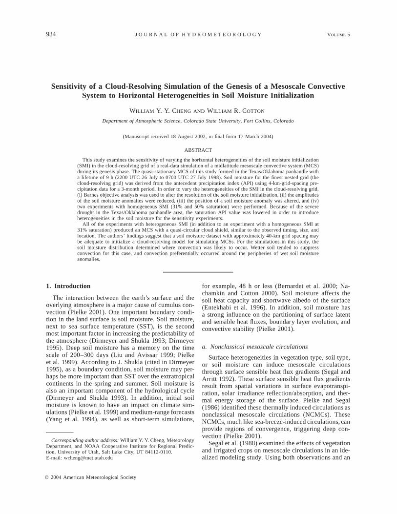
To determine the depth of the mesohigh generated byS2, we took a cross section of the horizontal temperaturedeviation through S2 at 26/1800 (Fig. 13). To obtain thetemperature deviation, we subtracted the temperaturefield from the average temperature at each constantheight level. Since the experiments with heterogeneousSMI had similar results, we will only show results fromexpt API. The depth of the cold pool associated withthe mesohigh generated by S2 was about 1.5 km, andits temperature deviation was on the order of 1 K. Thiscold pool suppressed convection because of its enhancedstability. However, acting as a focusing mechanism forconvection to develop, the leading edge of this cold poolresembled a sea breeze front, providing anomalous ver-tical motion around the periphery of S2 (Fig. 12).

d. Genesis phase: Grid 3

We examine the convective activity in the cloud-re-solving grid using the instantaneous precipitation rate.With the exception of expts APIMOVES2 and HOM50,all the experiments had very similar results at 26/1915(Fig. 14). There were two weak precipitation featuresin the western Oklahoma panhandle: C1 and C2, whichoriginally formed in the western Texas panhandle areaat 26/1500 as very weak precipitation features (;1 mmh21) and slowly moved northward. There was also astrong convective cell, C3, in the middle of the Texaspanhandle that formed in response to the build up ofCAPE and low-level convergence along the quasi-sta-tionary front. Compared to the satellite imagery at 26/1945 (Fig. 1b), the model placed the precipitation a bittoo far north and east of the Texas panhandle at this


FIG. 12. RAMS grid 3 vertical velocity difference at the lowest sz level above ground (thickcontours, every 2 cm s21) and sea level pressure difference (light contours, every 0.25 hPa) superposedwith the difference in horizontal wind vectors at the lowest sz level above ground at 26/1800 forexpts (a) API–HOM31, (b) API20–HOM31, (c) API40–HOM31, (d) API80–HOM31, (e) APIHALF–HOM31, (f ) APIMOVES2–HOM31, and (g) HOM50–HOM31. Solid (dashed) contours representpositive (negative) values, and zero contour is suppressed. Insets represent the scale of the windvectors in m s21.

time. Of note, at this time, the convection along thesurface trough in the Texas panhandle region (A2 in Fig.1b) was not captured by the model (see Fig. 3a). Thereare several possibilities for this. First, grid 3 (Fig. 2b)was not sufficiently large to cover the area where theconvective line A2 initiated (Fig. 1b). Second, grid 2

did not capture A2. Although grid 2 failed in this caseto capture A2, our experience with RAMS in real timesuggests that in some events, a horizontal grid spacingof 12 km is sufficient to resolve the gross features ofconvective events. Those cases are probably morestrongly forced than the case in this study in which a


FIG. 13. (a) Vertical cross section of horizontal temperature de-viation (at contour intervals of 0.25 K) taken through lines in Fig.11 for expts (a) API and (b) API80 at 26/1800. Zero contour issuppressed, and solid (dashed) contours represent positive (negative)values.

horizontal grid spacing of 12.5 km in grid 2 did nothave sufficient resolution to resolve A2. If grid 2 hadbeen able to capture the gross features of A2, grid 3might have been able to simulate A2 when it enters itsdomain. Third, the upper-level PV maximum (upstreamfrom the genesis region) missing in the model initiali-zation from the NCEP analysis (footnote 3) might havecaused the model not to initiate A2. Still, the timing ofthe model convection was reasonably good. Precipita-tion feature C2 was rather weak and would dissipateshortly after this time. Expt HOM31 (Fig. 14g) generatedresults similar to experiments with heterogeneous SMI(except for expt APIMOVES2). In expt APIMOVES2,the cooling effect of S2 suppressed the initiation of con-vective cell C3 at this time. In a similar manner, con-vection was suppressed in expt HOM50 at this time.Next, we examine how the soil moisture heterogeneitiesaffected the evolution of convection.

At 26/2145, convection was becoming more orga-nized for most of the experiments (Fig. 15). First, wediscuss the results in expts API, API20, API40, andAPI80. Qualitatively, expts API, API20, API40, andAPI80 had similar results. Precipitation feature C1 pre-cipitated more heavily with the smoothing of the SMIbecause of the enhanced NCMC associated with S1. TheNCMC generated by S2 provided a focusing mechanismfor convective features C3 and C4 to develop along theperiphery of S2 (Figs. 15a–d) because of the enhancedvertical motion there (Fig. 12). Convective feature C4

was generated 1 h earlier because of the remnant of theweak outflow boundary from C2 (Fig. 14) interactingwith the NCMC generated by the soil moisture anomalyS2. The outflow of C4 generated C7 ahead of it exceptin expt API40 in which C7 emerged 30 min later. Con-vective cell C6 was created when the NCMCs generatedby the northern and southern ends of S4 collided. Theoutflow from C3 also assisted in the initiation of C6. As

S4 was smoothed, leading to a reduction of its associatedNCMC, C6 was reduced in intensity.

Next, we discuss the results for the other experimentsat 26/2145 (Figs. 15e–h). In expt APIHALF, with S2 athalf its magnitude as in expt API, the NCMC associatedwith S2 was weaker. As a result, the enhanced verticalmotion around S2 was much smaller (Fig. 12). Thus, C3

and C4 did not track around S2 as much, but movedcloser to the interior of the much drier S2. Convectivecell C6 did not form because the NCMC associated withS4 was negligible. Expt APIMOVES2 produced resultsqualitatively similar to expt API, but C3 did not appear.Convective cell C6 in expt APIMOVES2 was also weak-er than that of expt API because of the absence of theoutflow boundary associated with C3 interacting withthe NCMC of S4. In expt HOM31, because of lack ofNCMC (from S2) interacting with C3, C3 could crossthe Oklahoma panhandle more easily. Convective cellC6 was expectedly absent in expt HOM31 because ofthe lack of soil moisture anomaly S4. Convection wasfinally initiated in expt HOM50 at this time, includingthe appearance of a multicellular system in the middleof the Texas/Oklahoma border. The delay in convectionin expt HOM50 was due to a cooler surface associatedwith a higher SLHF, making convection harder to ini-tiate.

By 26/2300, in all the experiments (except exptHOM50), the outflow boundaries of various cells havemerged into a convective line with a southeast–north-west orientation, just north of the Oklahoma panhandle(Fig. 16). The convective lines in expts API, API20,API40, and API80 were very similar to each other. Be-cause of the weaker NCMC from S2 interacting withthe convective line in expt APIHALF, the convectiveline advanced farther into the eastern edge of the do-main. The convective line in expt APIMOVES2 was abit shorter compared to other experiments because ofthe absence of C3 (Figs. 14 and 15). Qualitatively, theconvective line in expt HOM31 was similar to that inother experiments, but expt HOM50 failed to developa convective line. Also, convection was not well or-ganized in expt HOM50.

The time series of grid 3 domain-averaged SLHFshow expt HOM50 (APIHALF) to have the highest(lowest) SLHF (Fig. 17a). This is not surprising sincethe stomatal response function (a parameter controllingevapotranspiration; Avissar and Pielke 1991; Golaz etal. 2001) was almost unity (zero) for most of the do-main in expt HOM50 (APIHALF), allowing the most(the least) transpiration. All the other experiments fellsomewhere between the two extremes. Expt HOM31had slightly lower SLHF than expts API, API20,API40, API80, and APIMOVES2 between 26/1600 to26/2100. The SSHF time series (Fig. 17b) reveal acompletely opposite trend as compared to the latentheat time series because of the influence of soil mois-ture in partitioning the SSHF and SLHF. The highest(lowest) sensible heat flux was from expt APIHALF


FIG. 14. RAMS grid 3 precipitation rate (at contour intervals of 1, 5, 10, 20, 40, 80, and 120mm h21) at 26/1915 for expts (a) API, (b) API20, (c) API40, (d) API80, (e) APIHALF, (f )APIMOVES2, (g) HOM31, and (h) HOM50. Dashed contour represents initial volumetric soilmoisture at 50% saturation.

(HOM50), and the rest of the experiments again fellsomewhere in between. Although expt HOM50 had acolder surface temperature (ø4 K; not shown) thanexpt APIHALF because of a lower SSHF, expt HOM50had the highest CAPE because of a compensating in-

crease in low-level humidity (Fig. 17c). On the otherhand, although expt APIHALF had a warmer surfacetemperature than expt HOM50, the lower SLHF (hencereduced low-level humidity) resulted in a much lowervalue of CAPE. The other experiments fell somewhere


FIG. 15. As in Fig. 14, but for 26/2145.

in between the two extremes, but were closer to exptAPIHALF.

In the grid 3 domain-averaged precipitation rate timeseries (Fig. 18a), expt HOM50 had the lowest precip-itation rate among all the experiments, although it hadthe highest CAPE. Because of a higher SSHF in exptsAPIHALF and HOM31 (therefore warmer surface tem-

perature), the peak precipitation rate (hence peak con-vective activity) was reached 30 min sooner than exptsAPI, API20, API40, and API80. Also, in general, exptsAPIMOVES2 and HOM31 had lower precipitation ratesthan expts API, API20, API40, and API80. In terms ofthe grid 3 domain-averaged accumulated precipitationtime series, not surprisingly, expt HOM50 had the low-


FIG. 16. As in Fig. 14, but for 26/2300.

est accumulated precipitation because of a delay in con-vection and precipitation being confined to limited areasof the domain. Expt APIHALF had almost 1 mm higheraccumulated precipitation than expts API, API20,API40, API80, and HOM31 for about 30 min between26/2300 and 26/2330. Because of the suppressed for-mation of C3 in expt APIMOVES2, the accumulated

precipitation in expt APIMOVES2 was lower than thosein expts API, API20, API40, and API80.

As an evaluation of the simulated accumulated pre-cipitation, we compare the expt API 3-h accumulatedprecipitation in grid 3 with the data from the GCIParchive. There was little precipitation in the Texas pan-handle in grid 3 (contrary to the 3-h accumulated pre-


FIG. 17. Time series of grid 3 domain-averaged (a) surface latentheat flux (W m22); (b) surface sensible heat flux (W m22); and (c)CAPE (J kg21). Expt API is represented by the solid curve. Symbolsfor the other experiments are indicated.

FIG. 18. Time series of grid 3 domain-averaged (a) precipitationrate (mm h21) and (b) accumulated precipitation (mm). Expt API isrepresented by the solid curve. Symbols for the other experimentsare indicated.

cipitation from the GCIP archive in Fig. 19). As men-tioned previously, the model did not capture the initi-ation of the convective line A2 in the Texas panhandleand its subsequent development and northward advance-

ment (Fig. 1). Therefore, most of the convective pre-cipitation was too far north into Kansas. The accumu-lated precipitation from other experiments also did notcorrespond exactly to observations. Nevertheless,RAMS reproduced some aspects of the observed MCS;that is, RAMS simulated a cloud shield of similar sizeand shape near the right place and time as compared toobservations.

5. Discussion

In this study, the soil moisture distribution determinedwhere convection was likely to occur. From the accu-mulated precipitation field (Fig. 19), as well as the pre-cipitation rates (Figs. 14–16), it is clear that the NCMCsfrom the large soil moisture anomalies (e.g., S2) tendedto preferentially favor the convective cells to developaround their peripheries in this case. In other words,wetter soil contributes to a negative feedback in sub-sequent convective precipitation over the wetter soil. As


FIG. 19. The 3-h accumulated precipitation (mm) from 26/2100to 27/0000 for (a) expt API and (b) 4-km GCIP precipitation da-tabase.

we have seen in expt APIMOVES2, wetter soil tendsto suppress convection. Thus once the soil is wet, it isdifficult for it to receive convective precipitation or ini-tiate convection. In a two-dimensional (x–z) experiment(with a horizontal grid spacing of 2 km), Emori (1998)found that convection preferentially occurs on dry soil.Lynn et al. (1998) also found similar results as Emoriin a 2D cumulus ensemble model. Although Emori andLynn et al.’s results agreed with ours, a three-dimen-sional model would be needed to accurately representthe interaction of convection cells with the NCMCs in-duced by the soil moisture anomalies (e.g., the convec-tive cells tracking along the periphery of S2). As theMCS becomes more organized, with greater horizontalextent, we expect the NCMCs of the soil moisture anom-alies to be less effective in influencing the developmentof the MCS.

Observational studies from Segal et al. (1989) andRabin et al. (1990) also show that convection and cloud-iness tend to be suppressed over regions of high latent

heat flux. In Segal et al.’s study, the temperature dropand moisture increase were observed up to 445 m AGLover irrigated areas. The maximum contrast between theirrigated areas and surroundings was on the order of 10K. However, Segal et al. did not observe a sharply de-fined NCMC as anticipated because of the masking bythe background flow. Rabin et al. investigated the in-fluence of landscape variability in the initiation and de-velopment of cumulus clouds in Oklahoma. They ob-served that clouds formed the earliest over areas of highsensible heat flux, and cloud formation was suppressedover areas of high latent heat flux.

Our results from this case are in agreement with theobservational studies of Segal et al. (1989) and Rabinet al. (1990) and the 2D modeling studies of Emori(1998) and Lynn et al. (1998) in demonstrating a neg-ative feedback between convective precipitation and wetsoil during the genesis phase of the MCS. However,under different atmospheric conditions, the feedback be-tween convective precipitation and wet soil may be dif-ferent. For example, in one 1999 case, the simulationswere not sensitive to the soil moisture initialization be-cause of the unstable atmospheric conditions (notshown). In a counterexample to the aforementionedcase, Gallus and Segal (2000) found that convectiveprecipitation was sensitive in a simulation (with CAPEover 5500 J kg21 in some areas) to both the soil moistureand the CPS used. Gallus and Segal found that wettersoil generally produced a smaller precipitation maxi-mum in the experiments with K–F CPS because thetrigger function in the K–F CPS depends on the verticalvelocity. In the experiments with the Betts–Miller–Jan-jic (BMJ; Betts and Miller 1986; Janjic 1994) CPS,wetter soil produced a larger precipitation maximumbecause the BMJ is sensitive to the low-level and mid-level humidity. Also, in the K–F CPS, the convergenceof the parameterized downdrafts with the ambient flowover drier soil produced rainfall that was nonexistent inthe experiments using the BMJ CPS due to the lack ofparameterized downdrafts.

Using a one-dimensional model, Findell and Eltahir(2003a) determined the likelihood of convection as afunction of the convective triggering potential (CTP)and the low-level humidity (HIlow) in the early morningsounding and the soil moisture condition. The CTP iscomputed from integrating the area between the envi-ronmental temperature profile and a moist adiabat drawnupward from the observed temperature 100 hPa abovethe surface to a point 300 hPa above the surface. Thelow-level humidity HIlow is the sum of the dewpointdepressions at 50 and 100 hPa above the surface. Severalpossibilites can occur depending on the initial earlymorning sounding: (i) deep convection is favored overdry soil (dry soil advantage); (ii) deep convection isfavored over wet soil (wet soil advantage); and (iii)convection is atmospherically controlled (Fig. 20). Us-ing the aforementioned definitions of CTP and HIlow,we found that the grid 3 average of CTP and HIlow to


FIG. 20. The CTP–HIlow framework for describing atmospheric con-ditions in soil moisture–rainfall feedback [taken from Fig. 15 of Fin-dell and Eltahir (2003a)].

be 250 J kg21 and 15 K, respectively, at the model initialtime. These values fall near the boundary between (i)deep convection favored over dry soil and (ii) deepconvection unfavorable because of dry lower atmo-sphere (Fig. 20). Results from expts HOM31 andHOM50 (with homogeneous SMI)6 are not inconsistentwith the theory from Findell and Eltahir (2003a), withconvection being delayed and less widespread in grid 3in expt HOM50 (wetter soil) as compared to exptHOM31 (drier soil) (Figs. 14, 15, and 16).

Using multiyear summer (June, July, and August) ra-diosonde data for the continental United States, Findelland Eltahir (2003b) computed the CTP and HIlow forvarious stations and classifed the stations according tothe various regimes in the CTP–HIlow space as in Findelland Eltahir (2003a). For example, Texas/Oklahoma pan-handle falls within the regimes of (i) transition regionbetween wet and dry soil advantage, (ii) atmosphericallycontrolled region, and (iii) dry soil advantage. The GreatPlains region, to the lee of the Rockies, falls within theregimes of (i) the transition region between wet and drysoil advantage and (ii) the atmospherically controlledregion. To the east of the Great Plains, the region fallswithin the regime of wet soil advantage. The genesisphase of the simulated MCS (expts HOM31 andHOM50) in this case more or less falls under one ofthe categories determined by Findell and Eltahir (2003b)in the Texas/Oklahoma region: the category of dry soiladvantage. Although interesting, it is beyond the scopeof this paper to verify whether convection/soil moisturefeedback behaves differently in different regions of thecontinental United States because of the different ther-modynamic conditions. Earlier 1D model studies such

6 Since the theory of Findell and Eltahir (2003a) is based on a 1Dmodel, a comparison with experiments using homogeneous SMI ismore appropriate.

as Clark and Arritt (1995) and Segal et al. (1995) havealso discovered the nonlinearity of the soil moistureatmosphere inteaction. However, the conceptual modelof Findell and Eltahir (2003a,b) provides a more unifiedpicture of the soil moisture–atmosphere interaction.

The convective precipitation–soil moisture feedbackmechanism [in our study as well as those of Emori(1998) and Lynn et al. (1998)] differs from the feedbackof the large-scale flow and the soil moisture distribution.Namias (1959) was one of the first to suggest fromobservations that the soil moisture anomalies could as-sist in maintaining the persistence of large-scale at-mospheric circulation anomalies and vice versa. Ananomalous trough over a moist soil area prevents thebuildup of an upper-level ridge, and regions of dry soil(as a result of drought) are associated with an anomalousupper-level ridge. Therefore, over the drier (moist) soilarea, there would be reduced (increased) precipitationand maintenance of the dry (moist) soil conditions. Cas-telli and Rodriguez-Iturbe (1995) supported the findingof Namias (1959) using a semigeostrophic model. Theyfound that when the warm–moist (cold–drying) precip-itation anomaly of the baroclinic wave develops on topof a wetter (drier) soil, frontal collapse is reached soonerand the estimated precipitation greater.

Convection started at the same time in grid 3 for mostof the experiments, and the morphology of the convec-tive line was similar in most of the experiments. Evenexpt HOM31 (with homogeneous SMI at 31% satura-tion) produced results similar to those with heteroge-neous SMI. Expt API80 (while still retaining soil mois-ture patches of approximately 40 km in horizontal scale)generated results very similar to those in expt API, albeitwith weaker precipitation in some areas as compared toexpt API. So, there is little gain in providing SMI finerthan approximately 40 km in horizontal scale. This in-dicates the importance of large-scale dynamics. SomeMCSs are weakly forced by their large-scale environ-ments (e.g., Stensrud and Fritsch 1993), and we canonly speculate that small-scale soil moisture anomalieswould have a greater impact in those cases.

6. Conclusions

Using the API method to obtain soil moisture, wetested the sensitivity of varying the soil moisture ini-tialization on the cloud-resolving grid (2.5-km horizon-tal grid spacing) of a real-data MCS simulation. Becauseof the severe drought in the Texas/Oklahoma panhandle,we had to lower the saturation API value in order tointroduce heterogeneities in the soil moisture for thesensitivity experiments. The API soil moisture was ex-aggerated to test the maximum impact of the effects ofthe SMI. In the sensitivity experiments, we smoothedthe initial soil moisture in the cloud-resolving grid withBarnes objective analysis, using a response amplitudeof 0.5 and cutoff wavelengths of 20, 40, and 80 km. Inaddition, we also varied the soil moisture in amplitude


and displaced a soil moisture anomaly from its initiallocation. We also ran two experiments with homoge-neous soil moisture initialization at 31% and 50% sat-uration. Except for expt HOM50, RAMS simulated acloud shield, similar in location, timing, and size ascompared to observations. However, the accumulatedprecipitation did not compare as well to observations.Our findings are summarized below.

• Smaller soil moisture anomalies are more easilysmoothed out by the objective analysis filter. As aresult, smaller soil moisture anomalies are not wellrepresented in the smoothed soil moisture initializa-tion (i.e., with cutoff wavelength of 80 km), whichcan lead to underestimating NCMCs and precipitation(associated with the NCMCs).

• In this simulation, the soil moisture distribution de-termined where convection was likely to occur. Wettersoil had a tendency to suppress convection. In addi-tion, the NCMCs induced by the wet soil moistureanomalies provided a focusing mechanism for con-vection to develop along the peripheries of the wetsoil moisture anomalies due to the enhanced verticalmotion there. As a result, there existed a negativefeedback between wet soil and convective precipita-tion. However, we expect the NCMCs to be less ef-fective in influencing the development of the MCS asthe MCS becomes more organized (i.e., larger in ex-tent). Note that under certain atmospheric conditions,the negative feedback obtained here between wet soiland convection may not hold, as noted in other relatedstudies discussed further in section 5.

• In this case, large-scale forcing, in the form of a quasi-stationary front, provided a favorable environment forconvection to develop in this simulation. Thus, evenexpt HOM31 (with homogeneous SMI at 31% satu-ration) produced results similar to those with hetero-geneous SMI. Also, expt API80 (while still retainingsoil moisture patches of approximately 40 km in hor-izontal scale) had results very similar to those in exptAPI, albeit with weaker precipitation in some areasas compared to expt API. So, there is little gain inproviding SMI finer than approximately 40 km in hor-izontal scale.

Acknowledgments. This research was funded byNOAA under Grant NA67RJ0152 Amend 34. The au-thors wish to thank Prof. Roger Pielke Sr. for suggestingthe use of the NDVI dataset. The first author would alsolike to thank his Ph.D. committee members, Profs. ScottDenning, Paul Mielke, and Roger Pielke Sr. for theirsuggestions. We also thank Dr. Ken Mitchell and threeanonymous reviewers for their helpful comments in im-proving this manuscript. Thanks go to Kevin Schaeferand Joe Eastman for their help in working with theNDVI data. The help from Chris Rozoff with LATEXis much appreciated. Finally, we also thank RayMcAnnely for processing the satellite data, Steve Sa-

leeby for providing the code for the API calculation,and Brenda Thompson for proofreading and processingthe manuscript, respectively. The NDVI dataset was pro-vided by Brad Reed and Susan Maxwell of USGS, andthe satellite data was provided by the Global HydrologyResource Center.

APPENDIX

The Antecendent Precipitation Index

In this appendix, we present the algorithm for con-verting the API to volumetric soil moisture in grid 3.We used the EDAS soil moisture for grids 1 and 2. Thevolumetric soil moisture content (W) is the ratio of thevolume of water (Vw) in the soil versus the total volume(Vt) of the soil:

VwW 5 . (A1)Vt

The API on the nth day is given by

(API) 5 R 1 k(API) ,n n n21 (A2)

where the API value on the nth day depends on therainfall accumulation on the nth day (Rn), the depletioncoefficient (k), and the API value on the (n 2 1)th day.The depletion coefficient (from Lee 1992) has a timedependence to account for the seasonality:

(t 2 t 2 t )1 2k 5 1 2 0.04 sin 2p 1 1 , (A3)5 6[ ]t 0

where t is the time in Julian days, t1 is 15 days, t2 is91.25 days, and t0 is 365 days. The sinusoidal functionalform of k comes from Choudhury and Blanchard(1983). It is easy to see that the API on the nth day isthe weighted sum of n days of rainfall accumulation,and k normally ranges between 0.85 and 0.98 (Shaw1994).

To compute the fractional soil moisture (wfrac), weuse the following expression:

APInw 5 , (A4)frac APImax

where APImax is the maximum API value possible. Ac-cording to Chang and Wetzel (1991), the maximum API(centimeters) can be estimated by

21API 5 (1 2 k) .max (A5)

Using Lee’s (1992) formula for k, the average k for ourstudy is 0.93. Using the above equation from Chang andWetzel (1991) and a k of 0.93, the maximum API is140 mm. Because of the dry soil conditions, we loweredAPImax to 40 mm because we wanted to introduce het-erogeneities in the SMI. Despite the artificial introduc-tion of moist soil anomalies, the grid 3 soil moisturefor expt API remained quite dry, with a domain-aver-aged value of only 31% saturation. Luo et al. (2003)


found the lowest mean volumetric soil moisture in the0–40-cm layer during the May–July 1998 drought inOklahoma to be about 50% saturation. Thus, this arti-ficial increase in soil moisture is not that unrealistic, atleast in the domain-averaged sense. The API method isbetter at estimating near soil moisture rather than deep-layer soil moisture. As discussed in section 3b, we as-sumed the initial soil moisture to be invariant withdepth.

We performed two 15-h simulations in which the grid3 soil moisture deeper than 0.52 m in expt API (seeTable 2) was increased by 20% and 40%, respectively,while keeping the maximum soil moisture at 100% sat-uration. However, we found that two aforementionedexperiments did not differ substantially from expt API.So, the assumption of constant soil moisture with depthin grid 3 did not have a large impact on the simulations.

Note that the soil-type dataset has not yet been im-plemented in RAMS. We chose sandy clay loam as thesingle soil type for the entire model because it has anintermediate texture as compared to the soil types in thecentral United States (see Foth and Schafer 1980; Fastand McCorcle 1991).

To calculate the volumetric soil moisture, we multiplywfrac by the saturation volumetric moisture content (0.42m3 m23) for the sandy clay loam soil type. In saturatedsoil, all the pore spaces in the soil are occupied, andthe soil cannot hold additional water (Shaw 1994). Weconstrained the minimum volumetric soil moisture to avalue of 0.1 m3 m23 when converting the API to vol-umetric soil moisture. This minimum soil moisture valueis within the minimum range in the Oklahoma Mesonet.We interpolated the soil moisture to grid 3 by using abicubic spline interpolation (Vetterling et al. 1992).

REFERENCES

Ashby, C. T., W. R. Cotton, and R. McAnelly, 2001: Impact of soilmoisture initialization on a simulated flash flood. Preprints, 15thConf. on Precipitation Extremes: Prediction, Impacts, and Re-sponses, Albuquerque, NM, Amer. Meter. Soc., 260–263.

Avissar, R., and R. A. Pielke, 1991: The impact of plant stomatalcontrol on mesoscale atmospheric circulations. Agric. For. Me-teor., 54, 353–372.

Barnes, S. L., 1964: A technique for maximizing details in numericalweather map analysis. J. Appl. Meteor., 3, 396–409.

Basara, J. B., D. S. Arndt, H. L. Johnson, J. G. Brotzge, and K. C.Crawford, 1999: An analysis of the drought of 1998 using theOklahoma Mesonet. Eos, Trans. Amer. Geophys. Union, 79, 258.

Bell, G. D., and J. E. Janowiak, 1995: Atmospheric circulation as-sociated with the Midwest floods of 1993. Bull. Amer. Meteor.Soc., 76, 681–696.

——, M. S. Halpert, C. F. Ropelewski, V. E. Kousky, A. V. Douglas,R. C. Schnell, and M. E. Gelman, 1999: Climate assessment for1998. Bull. Amer. Meteor. Soc., 80, S1–S48.

Bernardet, L. R., and W. R. Cotton, 1998: Multiscale evolution of aderecho-producing mesoscale convective system. Mon. Wea.Rev., 126, 2991–3015.

——, L. D. Grasso, J. E. Nachamkin, C. A. Finley, and W. R. Cotton,2000: Simulating convective events using a high-resolution me-soscale model. J. Geophys. Res., 105, 14 963–14 982.

Betts, A. K., and M. J. Miller, 1986: A new convective adjustment

scheme. Part II: Single column tests using GATE wave, BOMEX,and arctic air-mass data sets. Quart. J. Roy. Meteor. Soc., 112,693–709.

Carlson, T. N., and D. A. Ripley, 1997: On the relation between NDVI,fractional vegetation cover, and leaf area index. Remote Sens.Environ., 62, 241–252.

Castelli, F., and I. Rodriguez-Iturbe, 1995: Soil moisture–atmosphereinteraction in a moist semigeostrophic model of baroclinic in-stability. J. Atmos. Sci., 52, 2152–2159.

Chang, J.-T., and P. J. Wetzel, 1991: Effects of spatial variations ofsoil moisture and vegetation on the evolution of a prestorm en-vironment: A numerical case study. Mon. Wea. Rev., 119, 1368–1390.

Chen, F., and R. Avissar, 1994a: The impact of land-surface wetnessheterogeneity on mesoscale heat fluxes. J. Appl. Meteor., 33,1323–1340.

——, and ——, 1994b: Impact of land-surface moisture variabilityon local shallow convective cumulus and precipitation in large-scale models. J. Appl. Meteor., 33, 1382–1401.

——, R. A. Pielke Sr., and K. Mitchell, 2001a: Development andapplication of land-surface models for mesoscale atmosphericmodels: Problems and promises. Observations and Modeling ofthe Land-Surface Hydrological Processes, V. Lakshmi, J. Al-berston, and J. Schaak, Eds., Amer. Geophys. Union, 107–135.

——, T. T. Warner, and K. Manning, 2001b: Sensitivity of orographicmoist convection to landscape variability: A study of the BuffaloCreek, Colorado, flash flood case of 1996. J. Atmos. Sci., 58,3204–3223.

Choudhury, B. J., and B. J. Blanchard, 1983: Simulating soil waterrecession coefficients for agricultural water sheds. Water Resour.Bull., 19, 241–247.

Clark, C. A., and R. W. Arritt, 1995: Numerical simulations of theeffect of soil moisture and vegetation cover on the developmentof deep convection. J. Appl. Meteor., 34, 2029–2045.

Cotton, W. R., and R. A. Anthes, 1989: Storm and Cloud Dynamics.Academic Press, 883 pp.

——, R. L. George, P. J. Wetzel, and R. L. McAnelly, 1983: A long-lived mesoscale convective complex. Part I: Mountain-generatedcomponent. Mon. Wea. Rev., 111, 1893–1918.

——, M.-S. Lin, R. L. McAnelly, and C. J. Trembeck, 1989: A com-posite model of mesoscale convective complexes. Mon. Wea.Rev., 117, 765–783.

——, and Coauthors, 2003: RAMS 2001: Current status and futuredirections. Meteor. Atmos. Phys., 82, 5–29.

Dalu, G. A., and R. A. Pielke, 1993: Vertical heat fluxes generatedby mesoscale atmospheric flow induced by thermal inhomoge-neities in the PBL. J. Atmos. Sci., 50, 919–926.

——, ——, R. Avissar, G. Kallos, M. Baldi, and A. Guerrini, 1991:Linear impact of thermal inhomogeneities on mesoscale atmo-spheric flow with zero synoptic wind. Ann. Geophys., 9, 641–647.

Dirmeyer, P. A., 1995: Problems in initializing soil wetness. Bull.Amer. Meteor. Soc., 76, 2234–2240.

——, and J. Shukla, 1993: Observational and modeling studies ofthe influence of soil moisture anomalies on the atmospheric cir-culation. Predictions of Interannual Climate Variations, J. Shuk-la, Ed., NATO ASI Series I, Vol. 6, Springer-Verlag, 1–23.

Ek, M. B., K. E. Mitchell, Y. Lin, P. Grunmann, E. Rogers, G. Gayno,and V. Koren, 2003: Implementation of the upgraded Noah land-surface model in the NCEP operational mesoscale Eta Model.J. Geophys. Res., 108, 8851, doi:10.1029/2002JD003296.

Emori, S., 1998: The interaction of cumulus convection with soilmoisture distribution: An idealized simulation. J. Geophys. Res.,103 (D8), 8873–8884.

Entekhabi, D., I. Rodriguez-Iturbe, and F. Castelli, 1996: Mutual in-teraction of soil moisture state and atmospheric processes. J.Hydrol., 184, 3–17.

Fast, J. D., and M. D. McCorcle, 1991: The effect of heterogeneoussoil moisture on a summer baroclinic circulation in the centralUnited States. Mon. Wea. Rev., 119, 2140–2167.


Findell, K. L., and E. A. B. Eltahir, 2003a: Atmospheric controls onsoil moisture–boundary layer interactions. Part I: Frameworkdevelopment. J. Hydrometeor., 4, 552–569.

——, and ——, 2003b: Atmospheric controls on soil moisture–boundary layer interactions. Part II: Feedbacks within the con-tinental United States. J. Hydrometeor., 4, 570–583.

Foth, H. D., and J. W. Schafer, 1980: Soil Geography and Land Use.John Wiley and Sons, 484 pp.

Fritsch, J. M., R. J. Kane, and C. R. Chelius, 1986: Contribution ofmesoscale convective weather systems to the warm-season pre-cipitation in the United States. J. Climate Appl. Meteor., 25,1333–1345.

Gallus, W. A., and M. Segal, 2000: Sensitivity of forecast rainfall ina Texas convective system to soil moisture and convective pa-rameterization. Wea. Forecasting, 15, 509–525.

——, and ——, 2001: Impact of improved initialization of mesoscalefeatures on convective system rainfall in 10-km Eta simulations.Wea. Forecasting, 16, 680–696.

Golaz, J.-C., H. Jiang, and W. R. Cotton, 2001: A large-eddy sim-ulation study of cumulus clouds over land and sensitivity to soilmoisture. Atmos. Res., 59–60, 373–392.

Grasso, L. D., 2000: A numerical simulation of dryline sensitivity tosoil moisture. Mon. Wea. Rev., 128, 2816–2834.

Harrington, J. Y., 1997: The effects of radiative and microphysicalprocesses on simulated warm and transition-season arctic stratus.Ph.D. dissertation, Colorado State University, 289 pp.

——, M. P. Meyers, R. L. Walko, and W. R. Cotton, 1995: Param-eterization of ice crystal conversion processes due to vapor de-position for mesoscale models using double-moment basis func-tions. J. Atmos. Sci., 52, 4344–4366.

——, T. Reisin, W. R. Cotton, and S. M. Kreidenweis, 1999: Cloudresolving simulations of Arctic stratus. Part II: Transition-seasonclouds. Atmos. Res., 51, 45–75.

Hong, S.-Y., and E. Kalnay, 2002: The 1998 Oklahoma–Texasdrought: Mechanistic experiments with NCEP global and re-gional models. J. Climate, 15, 945–963.

Janjic, Z. I., 1994: The step-mountain eta coordinate model: Furtherdevelopment of the convection, viscous sublayer, and turbulenceclosure model schemes. Mon. Wea. Rev., 122, 928–945.

Johnson, R. H., and P. J. Hamilton, 1988: The relationship of surfacepressure features to the precipitation and air flow structure ofan intense midlatitude squall line. Mon. Wea. Rev., 116, 1444–1472.

Kain, J. S., and J. M. Fritsch, 1990: A one-dimensional entraining/detraining plume model and its application in convective param-eterization. J. Atmos. Sci., 47, 2784–2802.

——, and ——, 1998: Multiscale convective overturning in meso-scale convective systems: Reconciling observations, simulations,and theory. Mon. Wea. Rev., 126, 2254–2273.

Kunkel, K. E., S. A. Changnon, and J. R. Angel, 1994: Climaticaspects of the 1993 Mississippi River basin flood. Bull. Amer.Meteor. Soc., 75, 811–822.

Kuo, S. L., 1974: Further studies of the parameterization of the effectof cumulus convection on large-scale flow. J. Atmos. Sci., 31,1232–1240.

Lee, T. J., 1992: The impact of vegetation on the atmospheric bound-ary layer and convective storms. Ph.D. dissertation, ColoradoState University, 137 pp.

Liu, Y., and R. Avissar, 1999: A study of persistence in the land–atmosphere system using a general circulation model and ob-servations. J. Climate, 12, 2139–2153.

Luo, L., and Coauthors, 2003: Validation of the North American LandData Assimilation System (NLDAS) retrospective forcing overthe Southern Great Plains. J. Geophys. Res., 108, 8843,doi:10.1029/2002JD003246.

Lynn, B. H., W.-K. Tao, and P. J. Wetzel, 1998: A study of landscape-generated deep moist convection. Mon. Wea. Rev., 126, 928–942.

Maddox, R. A., 1980: Mesoscale convective complexes. Bull. Amer.Meteor. Soc., 61, 1374–1387.

McAnelly, R. L., J. E. Nachamkin, W. R. Cotton, and M. E. Nicholls,1997: Upscale evolution of MCSs: Doppler radar analysis andanalytical investigation. Mon. Wea. Rev., 125, 1083–1110.

Meyers, M. P., R. L. Walko, J. Y. Harrington, and W. R. Cotton, 1997:New RAMS cloud microphysics parameterization. Part II: Thetwo-moment scheme. Atmos. Res., 45, 3–39.

Nachamkin, J. E., and W. R. Cotton, 2000: Interactions between adeveloping mesoscale convective system and its environment.Part II: Numerical simulation. Mon. Wea. Rev., 128, 1225–1244.

Namias, J., 1959: Persistence of mid-tropspheric circulations betweenadjacent months and seasons. The Atmosphere and the Sea inMotion, B. Bolin, Ed., Rockefeller Institute Press, 240–248.

Njoku, E., and D. Entekhabi, 1996: Passive microwave remote sens-ing of soil moisture. J. Hydrol., 184, 101–129.

Olsson, P. Q., and W. R. Cotton, 1997: Balanced and unbalancedcirculations in a primitive equation simulation of a midlatitudeMCC. Part I: The numerical simulation. J. Atmos. Sci., 54, 457–478.

Pielke, R. A., 2001: Influence of the spatial distribution of vegetationand soils on the prediction of cumulus convective rainfall. Rev.Geophys., 39, 151–177.

——, and M. Segal, 1986: Mesoscale circulations forced by differ-ential terrain heating. Mesoscale Meteorology and Forecasting,P. S. Ray, Ed., Amer. Meteor. Soc., 516–548.

——, T. J. Lee, J. H. Copeland, J. L. Eastman, C. L. Ziegler, and C.A. Finley, 1997: Use of USGS-provided data to improve weatherand climate simulations. Ecol. Appl., 7, 3–21.

——, G. E. Liston, J. L. Eastman, L. Lu, and M. Coughenour, 1999:Seasonal weather prediction as an initial value problem. J. Geo-phys. Res., 104, 19 463–19 479.

Rabin, R. M., S. Stadler, P. J. Webster, D. J. Stensrud, and M. Gregory,1990: Observed effects of landscape variability on convectiveclouds. Bull. Amer. Meteor. Soc., 71, 272–280.

Segal, M., and R. W. Arritt, 1992: Nonclassical mesoscale circulationscaused by surface sensible heat-flux gradients. Bull. Amer. Me-teor. Soc., 73, 1593–1604.

——, R. Avissar, M. C. McCumber, and R. A. Pielke, 1988: Eval-uation of vegetation effects on the generation and modificationof mesoscale circulations. J. Atmos. Sci., 45, 2268–2292.

——, W. Schreiber, G. Kallos, R. A. Pielke, J. R. Garratt, J. Weaver,A. Rodi, and J. Wilson, 1989: The impact of crop areas in north-east Colorado in midsummer mesoscale thermal circulations.Mon. Wea. Rev., 117, 809–825.

——, R. W. Arrit, C. Clark, R. Rabin, and J. Brown, 1995: Scalingevaluation of the effect of surface characteristics on potentialfor deep convection over uniform terrain. Mon. Wea. Rev., 123,383–400.

Sellers, P. J., C. J. Tucker, G. J. Collatz, S. O. Los, C. O. Justice, D.A. Dazlich, and D. A. Randall, 1994: A global 1 degree by 1degree NDVI data set for climate studies. Part 2: The generationof global fields of terrestrial biophysical parameters from theNDVI. Int. J. Remote Sens., 15, 3519–3545.

Shaw, E. M., 1994: Hydrology in Practice. 3d ed. Chapman and Hall,569 pp.

Stensrud, D. J., and J. M. Fritsch, 1993: Mesoscale convective sys-tems in weakly forced large-scale environments. Part I: Obser-vations. Mon. Wea. Rev., 121, 3326–3344.

Tripoli, G. J., and W. R. Cotton, 1982: The Colorado State UniversityThree-Dimensional Cloud/Mesoscale Model. Part I: General the-oretical framework and sensitivity experiments. Atmos. Res., 18,185–219.

Vetterling, W. T., S. A. Teukolsky, and W. H. Press, 1992: NumericalRecipes: Example Book (FORTRAN). Cambridge UniversityPress, 245 pp.

Walko, R. L., and Coauthors, 2000: Coupled atmosphere–biophysics–hydrology models for environmental modeling. J. Appl. Meteor.,39, 931–944.

Warner, T. T., and H. M. Hsu, 2000: Nested-model simulation of moistconvection: The impact of coarse-grid parameterized convection


on fine-grid resolved convection. Mon. Wea. Rev., 128, 2211–2231.

Weisman, M. L., W. C. Skamarock, and J. B. Klemp, 1997: Theresolution dependence of explicitly modeled convective systems.Mon. Wea. Rev., 125, 527–548.

Wetzel, P. J., W. R. Cotton, and R. L. McAnelly, 1983: A long-livedmesoscale convective complex. Part II: Evolution and structureof the mature complex. Mon. Wea. Rev., 111, 1919–1937.

Yan, H., and R. A. Anthes, 1988: The effects of variations in surfacemoisture on mesoscale circulations. Mon. Wea. Rev., 116, 192–208.

Yang, R., M. J. Fennessy, and J. Shukla, 1994: The influence of initialsoil wetness on medium-range surface weather forecasts. Mon.Wea. Rev., 122, 471–485.

Zhang, D.-L., K. Gao, and D. B. Parsons, 1989: Numerical sim-ulation of an intense squall line during 10–11 June 1985 PRE-STORM. Part I: Model verification. Mon. Wea. Rev., 117,960–994.

Zipser, E. J., 1982: Use of a conceptual model of the life cycle ofmesoscale convective systems to improve very-short-rangeforecasts. Nowcasting, K. Browning, Ed., Academic Press,191–204.

Documents

Sensitivity of a Cloud-Resolving Simulation of the …rams.atmos.colostate.edu/cotton/vita/149.pdf934 JOURNAL OF HYDROMETEOROLOGY VOLUME 5 q 2004 American Meteorological Society Sensitivity