Sensitivity of Northwest North Atlantic Shelf Circulation toSurface and Boundary Forcing: A Regional Model Assessment

Catherine E. Brennan* , Laura Bianucci†, and Katja Fennel

Department of Oceanography, Dalhousie University, Halifax, Nova Scotia, Canada

[Original manuscript received 30 September 2014; accepted 7 December 2015]

ABSTRACT The northwest North Atlantic shelves, influenced by both North Atlantic subpolar and subtropicalgyres, are among the most hydrographically variable regions in the North Atlantic Ocean and host biologicallyrich and productive fishing grounds. With the goal of simulating conditions in this complex and productiveregion, we implemented a nested regional ocean model that includes the Gulf of Maine, the Scotian Shelf, theGulf of St. Lawrence, the Grand Banks, and the adjacent deep ocean. Configuring such a model requires choosingexternal data to supply surface forcing and initial and boundary conditions, as well as the consideration of nestingoptions. Although these selections can greatly affect model performance and results, they are rarely systematicallyinvestigated. Here we assessed the sensitivity of our regional model to a suite of atmospheric forcing datasets, tosets of initial and boundary conditions constructed from multiple global ocean models and a larger scale regionalocean model, and to two variants of the model grid — one extending farther off-shelf and resolving Flemish Captopography. We conducted model simulations for a 6-year period (1999–2004) and assessed model performancerelative to a regional climatological dataset of temperature and salinity, to observations collected from multiplemonitoring stations and cruise transect lines, to satellite sea surface temperature (SST) data, to coastal sealevel estimates, and to descriptions and estimates of regional currents from literature. Based on this modelassessment, we determined the model configuration that best reproduces observations. We find that although allsurface forcing datasets are capable of producing model SSTs close to observed, the different datasets result insignificant differences in modelled sea surface salinity (SSS), with the European Centre for Medium-rangeWeather Forecasts’ (ECMWF) global atmospheric reanalysis (ERA-Interim) performing best. We also find thatinitial and boundary conditions based on global ocean models do not necessarily produce a realistic circulation,whereas using climatological initial and boundary conditions (constructed from long-term, monthly-mean outputfrom a larger scale regional model) improves model performance. Through this model assessment, we determinethe model configuration that best reproduces observations and gain generally applicable insight into the factorsthat are key to accurate model performance.

RÉSUMÉ [Traduit par la rédaction] Les plateaux nord-ouest de l’Atlantique Nord, sur lesquels influent à la foisles tourbillons subpolaire et subtropical de l’Atlantique Nord, figurent parmi les régions de cet océanaux propriétés hydrographiques les plus variables. De plus, ils comportent des zones de grande richesse biologiqueet productrices de poissons. Dans le but de simuler les conditions dans cette région complexe et productive, nousavons mis au point un modèle océanique régional imbriqué qui couvre le golfe du Maine, le plateau néo-écossais,le golf du Saint-Laurent, les grands bancs et la mer profonde adjacente. La configuration d’un tel modèle requiertla sélection de données externes qui reproduisent le forçage en surface, et les conditions initiales et limites, etnécessite l’évaluation d’options d’imbrication. Bien que ces éléments puissent grandement influer sur le rendementdu modèle et sur ses résultats, ils sont rarement évalués systématiquement. Nous examinons donc la sensibilité denotre modèle régional relativement à des données de forçages atmosphériques, à des conditions initiales et limitesconstruites à partir de multiples modèles océaniques mondiaux et d’un modèle océanique régional à grandeéchelle, ainsi qu’à deux variantes de la grille du modèle, dont une qui s’étend au-delà du plateau et qui reproduitla topographie du bonnet Flamand. La simulation couvre une période de 6 ans (1999 à 2004). Nous avons évalué lerendement du modèle en le comparant à des données climatologiques régionales de température et de salinité, àdes observations recueillies à de multiples stations de surveillance, à des données de transects relevées par bateau,à des températures marines en surface (SST) issues de satellites, à des estimations du niveau côtier de la mer, et àdes descriptions et estimations de courants régionaux provenant d’autres documents. Sur la base de cetteévaluation, nous avons déterminé la configuration du modèle qui reproduit le mieux les observations. Nousnotons que toutes les séries de données de forçage en surface peuvent produire des SST modélisées comparablesaux observations. En revanche, les diverses séries entraînent des différences considérables de salinité simulée à lasurface de la mer, bien que les réanalyses mondiales atmosphériques (ERA) du Centre européen pour lesprévisions météorologiques à moyen terme (ECMWF) aient montré un rendement supérieur. Nous constatons

*Corresponding author’s email: katie.brennan@dal.ca†Current affiliation: Coastal Sciences Division, Pacific Northwest National Laboratory, 1100 Dexter Ave. North, Suite 400, Seattle, WA, 98109, USA.

ATMOSPHERE-OCEAN iFirst article, 2016, 1–18 http://dx.doi.org/10.1080/07055900.2016.1147416Canadian Meteorological and Oceanographic Society

Dow

nloa

ded

by [

Dal

hous

ie U

nive

rsity

] at

06:

00 0

2 M

arch

201

6

aussi que les conditions initiales et limites provenant de modèles océaniques mondiaux ne produisent pasnécessairement une circulation réaliste, tandis que l’utilisation de conditions initiales et limites climatologiques(construites à partir de longues séries de sorties mensuelles moyennes issues d’un modèle régional à grandeéchelle) améliore le rendement du modèle. Grâce à cette évaluation, nous déterminons la configuration dumodèle qui reproduit le mieux les observations et nous acquérons des connaissances concrètes sur les facteursqui régissent principalement la qualité de la modélisation.

KEYWORDS Atlantic; circulation; dynamics; modelling; numerical

1 Introduction

The northwest North Atlantic is host to biologically rich andproductive fishing grounds. This high biological productivitymay be partly attributed to the large dynamic and geographiccomplexity characterizing the North Atlantic shelves, whichare influenced by both the North Atlantic subpolar and subtro-pical gyres (Loder, Petrie, & Gawarkiewicz, 1998), contain asemi-enclosed sea (e.g., Gulf of St. Lawrence) and importantcoastal currents (e.g., the Labrador Current), and exhibit thelargest observed sea surface temperature (SST) variability inthe North Atlantic (Thompson, Loucks, & Trites, 1988).Whether the shelf circulation in this complex region can be

well represented by global ocean models with low spatial res-olution is questionable. Several examples illustrate thatregional models have succeeded in simulating circulationand hydrography in sub-regions of the northwest North Atlan-tic — for the eastern Scotian Shelf (Han & Loder, 2003), theNewfoundland Shelf (Han, 2000; Han et al., 2008), the New-foundland and Labrador Shelves (Han, 2005), or the entireeastern Canadian shelf (Urrego-Blanco & Sheng, 2012). Inorder to simulate conditions in this productive and dynami-cally complex region, external data in the form of surfaceforcing and initial and boundary conditions are required, anddifferent options for model nesting must be considered. Theselection of forcing and boundary treatment holds the potentialto greatly affect model performance and results, but often thedifferent choices are not systematically investigated. Onerecent study investigated this downscaling problem for aregional model of the Middle Atlantic Bight by assessingmodel skill comparing three global models, four regionalmodels, and a regional climatology with observations(Wilkin & Hunter, 2013). Those authors found that a regionalclimatology performed as well as or better than the consideredocean models. Guo et al. (2013) evaluated downscaling ofmodel output for the Gulf of St. Lawrence region and foundthat removing biases in sea surface temperature (SST) resultedin improved surface temperature and wind estimates in theirmodel. Clearly, nesting choices can have a large impact onmodel performance and should be evaluated for each region.An even larger spread in model results resulting fromnesting choices for the northwest North Atlantic would beexpected (relative to the Middle Atlantic Bight) because ofits extreme variability and large dynamical complexity.Here we describe the implementation of a nested regional

ocean model for the northwest North Atlantic shelves, includ-ing the Gulf of Maine, the Scotian Shelf, the Gulf ofSt. Lawrence, the Grand Banks, and the adjacent deep

ocean. We assessed the sensitivity of our regional model toa suite of atmospheric forcing datasets, to sets of initial andboundary conditions constructed from different global oceanmodels and a larger scale regional ocean model, and to twovariants of the model grid — one extending farther off-shelfand resolving Flemish Cap topography. We additionallyevaluate the effect of including nudging of temperature andsalinity to the observed regional climatology of Geshelin,Sheng, and Greatbatch (1999). The goals of this model assess-ment are twofold: (i) to determine the model configuration thatbest reproduces observations, and (ii) to gain generally appli-cable insight into which factors are key to accurate modelperformance.

2 Model description

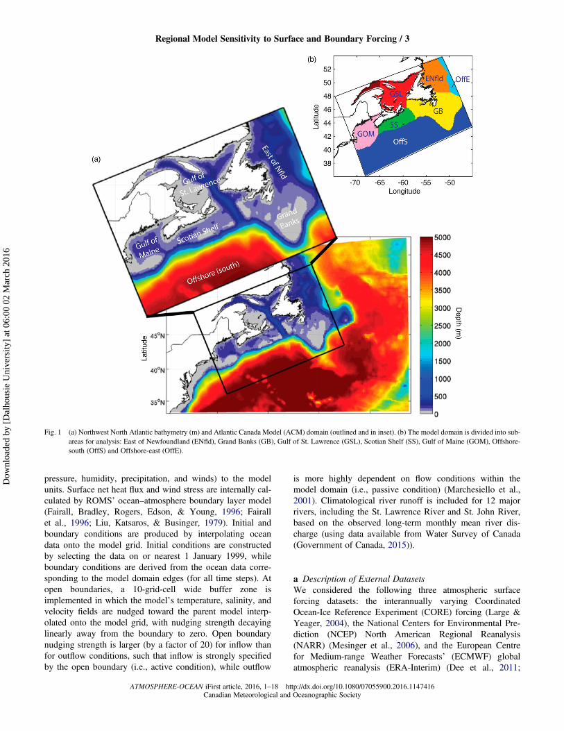
Our model, which we refer to as the Atlantic Canada Model(ACM), is based on the Regional Ocean Modelling System(ROMS), version 3.5, a terrain-following, free-surface, primi-tive equation ocean model (Haidvogel et al., 2008). The modeldomain includes the area between Cape Cod and the southerncoast of Labrador (Fig. 1a), encompassing the Gulf of Maine,Scotian Shelf, Gulf of St. Lawrence, Grand Banks, east New-foundland Shelf, and the deep-water region offshore to thesouth and east. The model’s 240-by-120 horizontal grid(�10 km horizontal resolution) is superimposed on theregion from 36.1°N to 53.9°N and 74.7°W to 45.1°W. TheACM is also tested on an expanded model domain (34.4°Nto 55.5°N and 74.7°W to 37.9°W, with a 300-by-150 horizon-tal grid at a similar �10 km resolution), which extends fartherto the east and south and additionally includes Flemish Cap.The model (for both grid versions) has 30 vertical levels andits minimum water depth is 10 m. The model employs thegeneric turbulence length-scale (GLS gen) vertical mixingscheme (Umlauf & Burchard, 2003; Warner, Sherwood,Arango, & Signell, 2005) and a combination of nudging andradiation open boundary conditions (Marchesiello, McWil-liams, & Shchepetkin, 2001). In its current set-up, the modeloutput is produced as five-day time averages, which we noteremoves the variability associated with synoptic weather.

Surface forcing, initial conditions, and boundary conditionsare provided from various external datasets (described inSection 2.a and Table 1). The ROMS interpolates surfaceforcing data from any regular grid and time step to themodel grid and time, and preliminary processing is limitedto converting surface forcing variables (e.g., shortwave radi-ation flux, longwave radiation flux, surface air temperature,

2 / Catherine E. Brennan et al.

ATMOSPHERE-OCEAN iFirst article, 2016, 1–18 http://dx.doi.org/10.1080/07055900.2016.1147416La Société canadienne de météorologie et d’océanographie

Dow

nloa

ded

by [

Dal

hous

ie U

nive

rsity

] at

06:

00 0

2 M

arch

201

6

pressure, humidity, precipitation, and winds) to the modelunits. Surface net heat flux and wind stress are internally cal-culated by ROMS’ ocean–atmosphere boundary layer model(Fairall, Bradley, Rogers, Edson, & Young, 1996; Fairallet al., 1996; Liu, Katsaros, & Businger, 1979). Initial andboundary conditions are produced by interpolating oceandata onto the model grid. Initial conditions are constructedby selecting the data on or nearest 1 January 1999, whileboundary conditions are derived from the ocean data corre-sponding to the model domain edges (for all time steps). Atopen boundaries, a 10-grid-cell wide buffer zone isimplemented in which the model’s temperature, salinity, andvelocity fields are nudged toward the parent model interp-olated onto the model grid, with nudging strength decayinglinearly away from the boundary to zero. Open boundarynudging strength is larger (by a factor of 20) for inflow thanfor outflow conditions, such that inflow is strongly specifiedby the open boundary (i.e., active condition), while outflow

is more highly dependent on flow conditions within themodel domain (i.e., passive condition) (Marchesiello et al.,2001). Climatological river runoff is included for 12 majorrivers, including the St. Lawrence River and St. John River,based on the observed long-term monthly mean river dis-charge (using data available from Water Survey of Canada(Government of Canada, 2015)).

a Description of External DatasetsWe considered the following three atmospheric surfaceforcing datasets: the interannually varying CoordinatedOcean-Ice Reference Experiment (CORE) forcing (Large &Yeager, 2004), the National Centers for Environmental Pre-diction (NCEP) North American Regional Reanalysis(NARR) (Mesinger et al., 2006), and the European Centrefor Medium-range Weather Forecasts’ (ECMWF) globalatmospheric reanalysis (ERA-Interim) (Dee et al., 2011;

Fig. 1 (a) Northwest North Atlantic bathymetry (m) and Atlantic Canada Model (ACM) domain (outlined and in inset). (b) The model domain is divided into sub-areas for analysis: East of Newfoundland (ENfld), Grand Banks (GB), Gulf of St. Lawrence (GSL), Scotian Shelf (SS), Gulf of Maine (GOM), Offshore-south (OffS) and Offshore-east (OffE).

Regional Model Sensitivity to Surface and Boundary Forcing / 3

ATMOSPHERE-OCEAN iFirst article, 2016, 1–18 http://dx.doi.org/10.1080/07055900.2016.1147416Canadian Meteorological and Oceanographic Society

Dow

nloa

ded

by [

Dal

hous

ie U

nive

rsity

] at

06:

00 0

2 M

arch

201

6

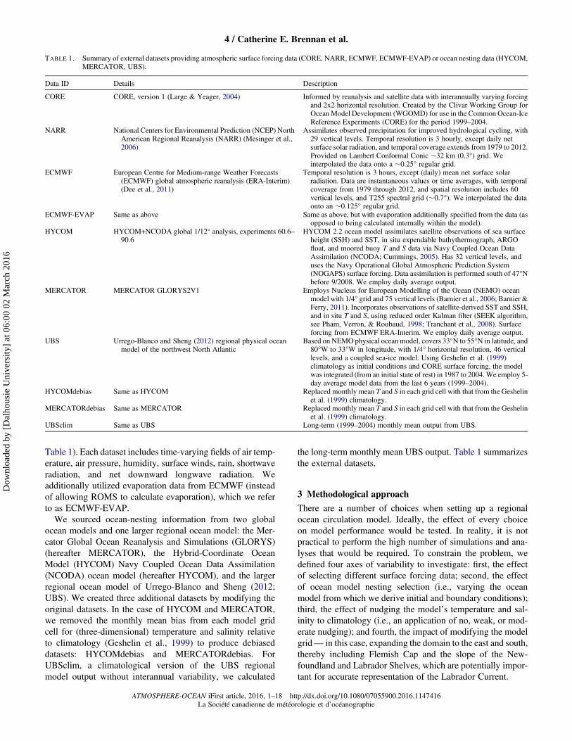
Table 1). Each dataset includes time-varying fields of air temp-erature, air pressure, humidity, surface winds, rain, shortwaveradiation, and net downward longwave radiation. Weadditionally utilized evaporation data from ECMWF (insteadof allowing ROMS to calculate evaporation), which we referto as ECMWF-EVAP.We sourced ocean-nesting information from two global

ocean models and one larger regional ocean model: the Mer-cator Global Ocean Reanalysis and Simulations (GLORYS)(hereafter MERCATOR), the Hybrid-Coordinate OceanModel (HYCOM) Navy Coupled Ocean Data Assimilation(NCODA) ocean model (hereafter HYCOM), and the largerregional ocean model of Urrego-Blanco and Sheng (2012;UBS). We created three additional datasets by modifying theoriginal datasets. In the case of HYCOM and MERCATOR,we removed the monthly mean bias from each model gridcell for (three-dimensional) temperature and salinity relativeto climatology (Geshelin et al., 1999) to produce debiaseddatasets: HYCOMdebias and MERCATORdebias. ForUBSclim, a climatological version of the UBS regionalmodel output without interannual variability, we calculated

the long-term monthly mean UBS output. Table 1 summarizesthe external datasets.

3 Methodological approach

There are a number of choices when setting up a regionalocean circulation model. Ideally, the effect of every choiceon model performance would be tested. In reality, it is notpractical to perform the high number of simulations and ana-lyses that would be required. To constrain the problem, wedefined four axes of variability to investigate: first, the effectof selecting different surface forcing data; second, the effectof ocean model nesting selection (i.e., varying the oceanmodel from which we derive initial and boundary conditions);third, the effect of nudging the model’s temperature and sal-inity to climatology (i.e., an application of no, weak, or mod-erate nudging); and fourth, the impact of modifying the modelgrid— in this case, expanding the domain to the east and south,thereby including Flemish Cap and the slope of the New-foundland and Labrador Shelves, which are potentially impor-tant for accurate representation of the Labrador Current.

TABLE 1. Summary of external datasets providing atmospheric surface forcing data (CORE, NARR, ECMWF, ECMWF-EVAP) or ocean nesting data (HYCOM,MERCATOR, UBS).

Data ID Details Description

CORE CORE, version 1 (Large & Yeager, 2004) Informed by reanalysis and satellite data with interannually varying forcingand 2x2 horizontal resolution. Created by the Clivar Working Group forOceanModel Development (WGOMD) for use in the Common Ocean-IceReference Experiments (CORE) for the period 1999–2004.

NARR National Centers for Environmental Prediction (NCEP) NorthAmerican Regional Reanalysis (NARR) (Mesinger et al.,2006)

Assimilates observed precipitation for improved hydrological cycling, with29 vertical levels. Temporal resolution is 3 hourly, except daily netsurface solar radiation, and temporal coverage extends from 1979 to 2012.Provided on Lambert Conformal Conic �32 km (0.3°) grid. Weinterpolated the data onto a �0.25° regular grid.

ECMWF European Centre for Medium-range Weather Forecasts(ECMWF) global atmospheric reanalysis (ERA-Interim)(Dee et al., 2011)

Temporal resolution is 3 hours, except (daily) mean net surface solarradiation. Data are instantaneous values or time averages, with temporalcoverage from 1979 through 2012, and spatial resolution includes 60vertical levels, and T255 spectral grid (�0.7°). We interpolated the dataonto an �0.125° regular grid.

ECMWF-EVAP Same as above Same as above, but with evaporation additionally specified from the data (asopposed to being calculated internally within the model).

HYCOM HYCOM+NCODA global 1/12° analysis, experiments 60.6–90.6

HYCOM 2.2 ocean model assimilates satellite observations of sea surfaceheight (SSH) and SST, in situ expendable bathythermograph, ARGOfloat, and moored buoy T and S data via Navy Coupled Ocean DataAssimilation (NCODA; Cummings, 2005). Has 32 vertical levels, anduses the Navy Operational Global Atmospheric Prediction System(NOGAPS) surface forcing. Data assimilation is performed south of 47°Nbefore 9/2008. We employ daily average output.

MERCATOR MERCATOR GLORYS2V1 Employs Nucleus for European Modelling of the Ocean (NEMO) oceanmodel with 1/4° grid and 75 vertical levels (Barnier et al., 2006; Barnier &Ferry, 2011). Incorporates observations of satellite-derived SST and SSH,and in situ T and S, using reduced order Kalman filter (SEEK algorithm,see Pham, Verron, & Roubaud, 1998; Tranchant et al., 2008). Surfaceforcing from ECMWF ERA-Interim. We employ daily average output.

UBS Urrego-Blanco and Sheng (2012) regional physical oceanmodel of the northwest North Atlantic

Based on NEMO physical ocean model, covers 33°N to 55°N in latitude, and80°W to 33°W in longitude, with 1/4° horizontal resolution, 46 verticallevels, and a coupled sea-ice model. Using Geshelin et al. (1999)climatology as initial conditions and CORE surface forcing, the modelwas integrated (from an initial state of rest) in 1987 to 2004.We employ 5-day average model data from the last 6 years (1999–2004).

HYCOMdebias Same as HYCOM Replaced monthly mean T and S in each grid cell with that from the Geshelinet al. (1999) climatology.

MERCATORdebias Same as MERCATOR Replaced monthly mean T and S in each grid cell with that from the Geshelinet al. (1999) climatology.

UBSclim Same as UBS Long-term (1999–2004) monthly mean output from UBS.

4 / Catherine E. Brennan et al.

ATMOSPHERE-OCEAN iFirst article, 2016, 1–18 http://dx.doi.org/10.1080/07055900.2016.1147416La Société canadienne de météorologie et d’océanographie

Dow

nloa

ded

by [

Dal

hous

ie U

nive

rsity

] at

06:

00 0

2 M

arch

201

6

We performed a number of model simulations for each setof model choices. In each simulation, the initial conditionsvary with the boundary conditions (i.e., the initial conditionsare derived from the same dataset as the boundary conditions).The simulations were conducted over the 6-year period 1999–2004. Runs performed using initial and boundary informationfrom the global HYCOM model are an exception becauseHYCOM output is only available beginning in November2003. The HYCOM-based runs span the years 2003 to2008. Although the later HYCOM time period could resultin different ocean states as a result of interannual variability,because we evaluate the model simulation with respect toobservations from 2003 to 2008, we expect any bias in themodel assessment to be minimized. A long simulation withUBSclim initial and boundary information was also performedover the period 1999–2008 (in order to compare with all othersimulations). The model simulations are listed in Table 2.We assessed model performance by comparing model

output with both observations and the climatologicalmonthly temperature and salinity dataset by Geshelin et al.(1999). Observations are from the Atlantic Zone MonitoringProgram (AZMP; Fisheries and Oceans Canada, 2011) andinclude conductivity-temperature-depth (CTD) measurementsfrom fixed monitoring stations and repeat cruise transectslocated on the Scotian Shelf, Gulf of St. Lawrence, GrandBanks, and the Newfoundland and Labrador Shelves (Ther-riault et al., 1998). We compared the AZMP data directlywith model temperature and salinity. For cruise transects,model output was sampled along each AZMP section at thecorresponding time; for monitoring stations, model outputwas sampled from the entire water column at the model grid

cell nearest each station, and the AZMP observations weredepth binned and averaged within each bin to correspond tothe model depths.

We also utilized satellite-derived SSTs. We used theAdvanced Very High Resolution Radiometer (AVHRR) Path-finder Level 3 Daily Daytime SST, Version 5, data product ona grid of approximately 0.044° (4 km resolution at the equator)for the years 1999–2006 (Kilpatrick, Podesta, & Evans, 2001;ftp://podaac-ftp.jpl.nasa.gov/allData/avhrr/L3/pathfinder_v5/daily/day). We also used the National Aeronautics and SpaceAdministration (NASA), Jet Propulsion Laboratory (JPL),Group for High Resolution Sea Surface Temperature(GHRSST) Level 4 Operational Sea Surface Temperature andSea Ice Analysis (OSTIA) Global Foundation SST AnalysisProduct (hereafter GHRSST) on a 0.054° grid (ftp://podaac-ftp.jpl.nasa.gov/allData/ghrsst/data/L4/GLOB/UKMO/OSTIA/)for the years 2007–2008.We note that there is an offset betweensummer SSTvalues determined using SSTvalues fromAVHRRand those from climatology (Geshelin et al., 1999): mainly, theAVHRR SSTs are warmer than climatology in summer. Theorigin of this seasonal bias is unknown. Although it mayappear sufficient to compare model SST results solely with theclimatological values of Geshelin et al. (1999), the climatologyis not necessarily independent of the model results. Forexample, the model is nudged to the climatology in runsACM-buff-GeshTS (nudging occurs only in the boundariesand buffer zone), ACM-buff-GeshTS-interior120day, andACM-buff-GeshTS-interior60day (nudging occurs at all modelgrid cells). Also, model runs employing UBS model data (e.g.,as initial and boundary conditions) are indirectly influenced bythe climatology because the UBS model is initialized from this

TABLE 2. Atlantic Canada model (ACM) simulations.

Run ID Surface Forcing Nesting Interior Nudging Grid

Vary Surface ForcingACM-CORE CORE UBSclim N/A OrigACM-NARR NARR UBSclim N/A OrigACM-ECMWF ECMWF UBSclim N/A OrigACM-ECMWF-EVAP ECMWF+EVAP UBSclim N/A OrigVary Nesting DataACM-UBS ECMWF UBS N/A OrigACM-UBSclim ECMWF UBSclim N/A OrigACM-HYCOM ECMWF HYCOM N/A OrigACM-MERCATOR ECMWF MERCATOR N/A OrigACM-HYCOMdebias ECMWF HYCOM debiased N/A OrigACM-MERCATORdebias ECMWF MERCATOR debiased N/A OrigVary NudgingACM-UBSclim ECMWF UBSclim N/A OrigACM-buff-UBSclimTS ECMWF UBSclim N/A OrigACM-buff-GeshTS ECMWF UBSclim N/A OrigACM-buff-GeshTS

-interior120dayECMWF UBSclim 120 day

(weak)Orig

ACM-buff-GeshTS-interior60day

ECMWF UBSclim 60 day(moderate)

Orig

Vary Model GridACM-Original ECMWF UBSclim N/A OrigACM-Large ECMWF UBSclim N/A Large

Note: ACM-UBSclim, ACM-Orig, and ACM-ECMWF are the same simulation.

Regional Model Sensitivity to Surface and Boundary Forcing / 5

ATMOSPHERE-OCEAN iFirst article, 2016, 1–18 http://dx.doi.org/10.1080/07055900.2016.1147416Canadian Meteorological and Oceanographic Society

Dow

nloa

ded

by [

Dal

hous

ie U

nive

rsity

] at

06:

00 0

2 M

arch

201

6

climatology and employs a spectral nudging method to the cli-matological dataset. TheAVHRRSSTdataset thus adds an inde-pendent point of comparison.We compared time series of model temperature and salinity,

at the sea surface and bottom, averaged over the entire modeldomain and for domain sub-areas (see Fig. 1b), with theregional climatological temperature and salinity (Geshelinet al., 1999). In order to compare model output directly withthe climatology, we interpolated the monthly climatologicaldata to the model time and the model grid. For SST, we alsocompared the simulated SST time series with satellite SSTs.In order to facilitate the comparison, we regridded highquality, daily AVHRR (GHRSST) SSTs onto the model grid(quality flag ≥4 and error flag ≤4°C for AVHRR andGHRSST, respectively). We discarded interpolated valueslocated more than 1/8° from the satellite observations. We cal-culated five-day averages of the interpolated satellite SST (tocompare directly with the model’s five-day time averages).Simulated and climatological SSTs were extracted only fromgrid cells where satellite data exist, then the domain-wideand sub-domain area averages were calculated (time seriesof salinity use all grid locations in the areal average). Wedetermined statistical metrics of bias, accuracy (root-mean-square error (RMSE)), and correlation (Pearson’s R2)between the simulated and observed values.Finally, we evaluated sea level and currents in the model

with respect to observations. We supplemented that quantitat-ive assessment with qualitative evaluation of simulated surfacevelocity fields using descriptions of key dynamical features inthe region from the literature. In order to compare sea level inthe model with observations, total sea level at multiple coastalmonitoring stations (Halifax, Yarmouth, Rimouski, Saint-Francois, Sept-Îles, and Charlottetown) was extracted fromthe Fisheries and Oceans Canada tide gauge dataset (Fisheriesand Oceans Canada, 2015; http://extrememarine.ocean.dal.ca/dalcoast/Canada.php) for the time period 1999–2001. Becausethe model does not include tides, the tidal component of sealevel at each station was estimated using a harmonic analysisof ocean tides (Pawlowicz, 2011; Pawlowicz, Beardsley, &Lentz, 2002). The tidal component was then removed fromthe total sea level (via differencing) to determine the non-tidal sea level at each monitoring station, which is directlycomparable to model sea level. We then compared the non-tidal sea level time series (1999–2001) at each monitoringstation with the closest model ocean grid point and computedstatistical measures of the time series’ performance for eachmodel simulation.As an alternative approach to assessing regional circulation

in the model, volume transports were determined at multiplelocations, including sections representing the LabradorCurrent and the Nova Scotia Current (NSC). Simulated long-term mean volume transports were compared with obser-vation-based estimates of annual mean transports from Loderet al. (1998). Modelled volume transports were calculated uti-lizing the criterion of S < 34.8 following Loder et al. (1998).Section locations were chosen in the model to correspond as

closely as possible to the sections listed by Loder et al.(1998) in their Table 1 and Fig. 5.2. These sections includethe Labrador Current at Hamilton Bank off the southern coastof Labrador (7.5 Sv (1 Sv=106 m3 s−1) from Lazier andWright (1993)), the Labrador Current transport throughFlemish Pass (5.8 Sv from Petrie and Buckley (1996)) andaround the Tail of the Grand Banks (3.2 Sv from Petrie andDrinkwater (1993)), and the NSC at the Halifax Section(0.70 Sv from Anderson and Smith (1989)). Because theHamilton Bank section from Loder et al. (1998) is situatedslightly north of the model domain’s northern edge, wecompare that volume transport with section LC1 locatedwithin our model domain and south of the model buffer zone.

In the following sections, we investigate the effects onmodel performance of varying surface forcing and modelnesting data, of nudging the model toward climatology, andof expanding the model grid.

4 Model assessment I: Effect of surface forcingselection

We performed four simulations differing only by the surfaceforcing dataset selected (Table 2). All simulations usedUBSclim ocean initial and boundary conditions. We refer tothese simulations as ACM-CORE, ACM-NARR, ACM-ECMWF, and ACM-ECMWF-EVAP. Below we assessthese model simulations.

Time series of area-averaged sea surface properties (temp-erature and salinity) are constructed for the entire modeldomain and the sub-areas shown in Fig. 1b. Salinity is com-pared with climatological values (Geshelin et al., 1999), andtemperature is compared with both climatology and anAVHRR satellite SST dataset. Figure 2 presents the timeseries of ACM-NARR, ACM-ECMWF, and ACM-COREwith those generated from climatology and the AVHRR data.

The surface time series averaged over the entire domain(Fig. 2a) and regions of the model domain (Fig. 2b) revealthat the model performs reasonably well using either NARRor ECMWF surface forcing. The statistical results are pre-sented in Table S1a (supplementary data). The domain-aver-aged SST is well correlated with the Geshelin climatology(AVHRR), with R2 values of 0.97 and 0.96 (0.99 and 1.00)for ACM-NARR and ACM-ECMWF, respectively. Seasonal-ity is generally well captured although the simulated winterSST is cooler than climatology and AVHRR. In summer,modelled SST lies between the climatological and satellitevalues (i.e., warmer than climatology but cooler than satelliteSST). Sea surface salinity (SSS) is also simulated well, withdomain-wide R2 values of 0.80 and 0.85 for ACM-NARRand ACM-ECMWF, respectively. Differences in SSS aremainly located in the Gulf of St. Lawrence, where ACM-NARR is fresher, and on the Scotian Shelf, where ACM-NARR is fresher from 2002 to mid-2003. We conclude thatboth ECMWF and NARR surface forcing result in good distri-butions of surface temperature and salinity in the model.

6 / Catherine E. Brennan et al.

ATMOSPHERE-OCEAN iFirst article, 2016, 1–18 http://dx.doi.org/10.1080/07055900.2016.1147416La Société canadienne de météorologie et d’océanographie

Dow

nloa

ded

by [

Dal

hous

ie U

nive

rsity

] at

06:

00 0

2 M

arch

201

6

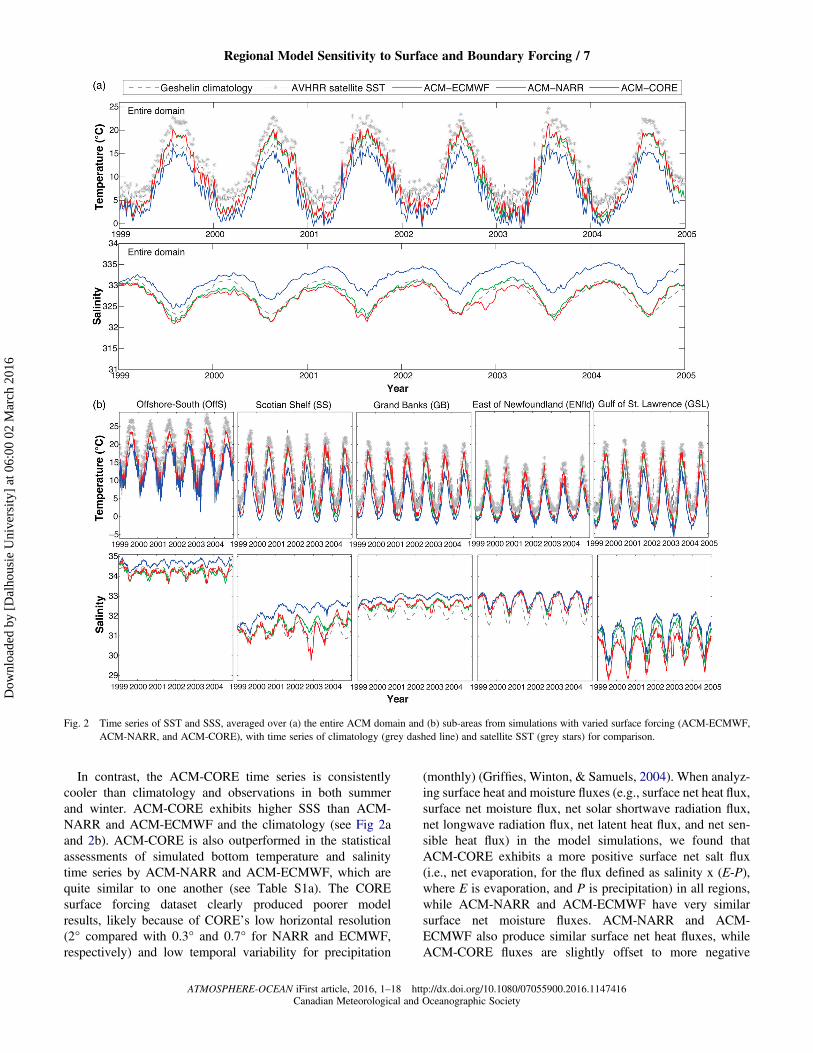
In contrast, the ACM-CORE time series is consistentlycooler than climatology and observations in both summerand winter. ACM-CORE exhibits higher SSS than ACM-NARR and ACM-ECMWF and the climatology (see Fig 2aand 2b). ACM-CORE is also outperformed in the statisticalassessments of simulated bottom temperature and salinitytime series by ACM-NARR and ACM-ECMWF, which arequite similar to one another (see Table S1a). The COREsurface forcing dataset clearly produced poorer modelresults, likely because of CORE’s low horizontal resolution(2° compared with 0.3° and 0.7° for NARR and ECMWF,respectively) and low temporal variability for precipitation

(monthly) (Griffies, Winton, & Samuels, 2004). When analyz-ing surface heat and moisture fluxes (e.g., surface net heat flux,surface net moisture flux, net solar shortwave radiation flux,net longwave radiation flux, net latent heat flux, and net sen-sible heat flux) in the model simulations, we found thatACM-CORE exhibits a more positive surface net salt flux(i.e., net evaporation, for the flux defined as salinity x (E-P),where E is evaporation, and P is precipitation) in all regions,while ACM-NARR and ACM-ECMWF have very similarsurface net moisture fluxes. ACM-NARR and ACM-ECMWF also produce similar surface net heat fluxes, whileACM-CORE fluxes are slightly offset to more negative

Fig. 2 Time series of SST and SSS, averaged over (a) the entire ACM domain and (b) sub-areas from simulations with varied surface forcing (ACM-ECMWF,ACM-NARR, and ACM-CORE), with time series of climatology (grey dashed line) and satellite SST (grey stars) for comparison.

Regional Model Sensitivity to Surface and Boundary Forcing / 7

ATMOSPHERE-OCEAN iFirst article, 2016, 1–18 http://dx.doi.org/10.1080/07055900.2016.1147416Canadian Meteorological and Oceanographic Society

Dow

nloa

ded

by [

Dal

hous

ie U

nive

rsity

] at

06:

00 0

2 M

arch

201

6

values (i.e., net heat loss, corresponding to ocean cooling),especially in the offshore region.The final surface forcing dataset, ECMWF-EVAP, allows

us to evaluate whether model performance can be improvedby specifying the reanalysis evaporative surface flux in themodel, as opposed to allowing ROMS to calculate evaporationas a function of air temperature and humidity. In the simu-lation employing evaporation data, ACM-ECMWF-EVAP,surface and bottom temperature are essentially unchanged,while SSS increases in the Offshore-South area, over theshelves including the Scotian Shelf and Grand Banks, and inthe Gulf of St. Lawrence, increasing the positive salinitybias over those regions (Fig. 3). The 2003 mean annual SSSanomaly relative to climatology is mapped in Fig. 3. Thenortheastern quadrant of the domain (Offshore-East andeastern Newfoundland Shelf) is unaffected. The R2 value forthe average SSS time series in the domain is reduced (to0.80 from 0.85 in ACM-ECMWF), and the RMSE is slightlyincreased (see Table S1a). Based on the statistical comparisonof model results with observations and climatology, we con-clude that specifying evaporation does not improve modelperformance.There are several model biases (relative to the climatology)

in the shelf regions that are common across simulations withvaried surface forcing (Fig. 2b, Table S1a). First, model SSSis higher in the eastern Newfoundland Shelf and easternGulf of St. Lawrence regions (small bias) and fresher in thelower St. Lawrence Estuary than observations. Bottom salinityis consistently too high in the western Scotian Shelf and toofresh on the eastern Scotian Shelf, such that the model’seast–west bottom salinity gradient on the Scotian Shelf isweaker than that indicated by the climatology. In terms ofbottom temperatures, the Grand Banks is too warm, and theeastern Scotian Shelf and Gulf of Maine are too cool. Nextwe assess how different ocean-nesting treatments, the

application of nudging, and changes in model grid affect theACM-NARR and ACM-ECMWF results.

5 Model assessment II: Effect of ocean model nesting

The effect of model nesting is investigated by varying the phys-ical initial and boundary information (temperature, salinity, vel-ocities, and sea surface height) provided to the ACM. Weperformed six simulations differing only in which ocean modelnesting dataset was selected (all utilize ECMWF surfaceforcing). We refer to these simulations as ACM-HYCOM,ACM-MERCATOR, ACM-UBS, ACM-HYCOMdebias,ACM-MERCATORdebias, and ACM-UBSclim (Table 2). Allsimulations are for the time period 1999–2004, except theHYCOM simulations because HYCOM data are only availablestarting inNovember 2003.We therefore performed simulationswith HYCOM data from 2003 to 2008 and conducted oneextended simulation (1999–2008) using regional model output(ACM-UBSclim-long) for comparison purposes.

Nesting the ACM in either of the global ocean models,HYCOM or MERCATOR, results in poor model perform-ance, irrespective of whether we utilize the original ordebiased initial and boundary datasets. We assessed model sal-inity and temperature along the AZMP cruise transects locatedin the model domain. Figure 4 depicts the vertical salinity dis-tribution along the Halifax Line transect in May 2004 in themodel and fromAZMP observations. The ACM-HYCOMdebiasand ACM-MERCATORdebias simulations produce a poorlysimulated shelf vertical structure: salinity is too high on theshelf (this is the case when using either debiased or non-debiased ocean-nesting datasets). The SSS biases andRMSEs are significantly higher in those simulations employ-ing initial and boundary conditions derived from HYCOMand MERCATOR (Table S1b).

Fig. 3 Mean annual SSS anomaly (model-climatology) in 2003.

8 / Catherine E. Brennan et al.

ATMOSPHERE-OCEAN iFirst article, 2016, 1–18 http://dx.doi.org/10.1080/07055900.2016.1147416La Société canadienne de météorologie et d’océanographie

Dow

nloa

ded

by [

Dal

hous

ie U

nive

rsity

] at

06:

00 0

2 M

arch

201

6

Although SSS is not well simulated when using HYCOM orMERCATOR boundary information, simulated SSTs are rea-listic. Averaged over the model domain, ACM-MERCATORexhibits the smallest RMSE and bias relative to satellite obser-vations and the climatological SST of all 6-year long simu-lations (Table S1b). ACM-HYCOM SST also performs well.When we compare ACM-HYCOM and ACM-HYCOMdebiasdirectly with ACM-UBSclim-long for the same time period(2004–2008), ACM-HYCOM exhibits the smallest RMSEof the three simulations in domain-averaged SST for both sat-ellite and climatology (RMSE = 1.56°C and 1.18°C, respect-ively). However, neither bottom temperature nor bottomsalinity is well represented by the model when initial andboundary conditions are provided by HYCOM,MERCATOR,or their debiased versions (Table S1b).In contrast to the simulations using initial and boundary

information sourced from global ocean models, ACM-UBSand ACM-UBSclim both simulate shelf conditions ade-quately. In ACM-UBS the vertical structure of salinity onthe Halifax Line is similar to AZMP observations (Fig. 4shows the comparison in May 2004) although the deepestshelf water (�150–175 m) is not as saline as observations.The ACM-UBS and ACM-UBSclim simulations producevery similar time series of temperature and salinity at thesurface and bottom averaged over all the sub-areas (notshown). Only small differences in SSS and bottom tempera-ture and salinity are found between the ACM-UBS andACM-UBSclim simulations. In the offshore regions theACM-UBS simulation is slightly saltier in winter and springthan the ACM-UBSclim simulation. On the Scotian Shelf,ACM-UBSclim exhibits slightly cooler and fresher bottomwaters relative to climatology (and the bottom waters on theScotian Shelf in the ACM-UBSclim are also fresher than inthe ACM-UBS simulation).

Both ACM-UBS and ACM-UBSclim perform well withrespect to climatology. Comparisons of the time series ofdomain-averaged SSS and SST to climatology show verysimilar statistical results. The ACM-UBSclim R2 values areincrementally higher for SSS (by 0.06) and identical for SST(see Table S1b). In the comparison with satellite SST,domain-averaged R2 values are identical (1.00), whereas theACM-UBSclim domain-averaged bias and RMSE increaseslightly (by 0.15°C). ACM-UBSclim exhibits small improve-ments in statistical metrics for bottom salinity and temperature(higher R2 values by 0.01 and 0.23, and lower RMSE by 0.03°and 0.06°C, respectively). However, small differences in thestatistical measures are likely not meaningful. Surface velocityfields (shown for year 2004 in Fig. 5) indicate that for ACM-MERCATOR, ACM-HYCOM, ACM-MERCATORdebias,and ACM-HYCOMdebias the Gulf Stream may be situatedtoo close to the shelf slope and that the annual mean shelfbreak current transport can occur toward the northeast,which is in the opposite direction from observed. The GulfStream in the southern portion of the domain is displacedfurther from the shelf break in ACM-UBSclim, and the shelfbreak current is stronger (Fig. 5). We conclude that of thevaried ocean-nesting set-ups, ACM-UBS and ACM-UBSclim perform best. We prefer to use the monthly climato-logical boundary conditions, UBSclim, over the 5-day varyingUBS because simulations using UBSclim are not confined tothe specific time period of the parent model.

We compared the simulations using debiased MERCATORand HYCOM datasets, ACM-MERCATORdebias and ACM-HYCOMdebias (which are debiased with respect to theGeshelin climatology), with the complete set of observationaldata, including AZMP measurements, satellite SST, and theGeshelin climatology. Here we note that the comparisonwith Geshelin climatology is not independent. Despite this,

Fig. 4 Model salinity along the Halifax Line transect, overlain by AZMP observations, in May 2004, for three simulations: ACM-HYCOMdebias, ACM-MER-CATORdebias, and ACM-UBS.

Regional Model Sensitivity to Surface and Boundary Forcing / 9

ATMOSPHERE-OCEAN iFirst article, 2016, 1–18 http://dx.doi.org/10.1080/07055900.2016.1147416Canadian Meteorological and Oceanographic Society

Dow

nloa

ded

by [

Dal

hous

ie U

nive

rsity

] at

06:

00 0

2 M

arch

201

6

debiasing does not improve the simulations’ bias relative toclimatology, as shown below.Debiasing the MERCATOR and HYCOM datasets pro-

duced mixed results. In the case of MERCATOR, debiasinghad no discernable effect on modelled SST, but improvedbottom temperature in most sub-regions (except the Gulf of

St. Lawrence and the Scotian Shelf). The SSS improvedgreatly in the easterly portion of the domain (Offshore-East,the Grand Banks, and the eastern Newfoundland Shelf), butonly slightly on the Scotian Shelf. Debiasing created negligibleimprovement in the lower St. Lawrence Estuary, the Gulf ofSt. Lawrence, and the Scotian Shelf where non-trivial bottom

Fig. 5 Annual mean surface velocity (m s−1) mapped in 2004 for each simulation with varying ocean nesting (ACM-UBS, ACM-UBSclim, ACM-MERCATOR,ACM-MERCATORdebias, ACM-HYCOM, and ACM-HYCOMdebias). Vector arrows (black) are drawn at identical locations for comparison.

10 / Catherine E. Brennan et al.

ATMOSPHERE-OCEAN iFirst article, 2016, 1–18 http://dx.doi.org/10.1080/07055900.2016.1147416La Société canadienne de météorologie et d’océanographie

Dow

nloa

ded

by [

Dal

hous

ie U

nive

rsity

] at

06:

00 0

2 M

arch

201

6

salinity biases exist. Some improvement in bottom salinity wasapparent in the Grand Banks and the eastern NewfoundlandShelf. Similar changes were identified in ACM-HYCOMde-bias, though bottom salinity in the Grand Banks and easternNewfoundland Shelf did not improve (as occurred in ACM-

MERCATORdebias). The SSS was again improved in theeastern portion of the domain in ACM-HYCOMdebias. Thenet improvement in bottom temperature in ACM-HYCOMde-bias likewise occurred in most regions (except in the ScotianShelf, Grand Banks, and eastern Newfoundland Shelf).

Fig. 6 The observed range of mean annual GSNW index locations (black outline with grey shading) (see Fig. 5 in Joyce et al., 2000) with the long-term meanposition of the ACM simulations (coloured lines) with (a) varied ocean nesting and (b) varied treatment of buffer zone nudging. The grey dashed line indi-cates the model grid boundary.

Regional Model Sensitivity to Surface and Boundary Forcing / 11

ATMOSPHERE-OCEAN iFirst article, 2016, 1–18 http://dx.doi.org/10.1080/07055900.2016.1147416Canadian Meteorological and Oceanographic Society

Dow

nloa

ded

by [

Dal

hous

ie U

nive

rsity

] at

06:

00 0

2 M

arch

201

6

We also explored the position of the Gulf Stream in themodel simulations with varied ocean nesting. We utilizedthe Gulf Stream North Wall (GSNW) index, followingJoyce, Deser, and Spall (2000), who defined this metric tobe the location of the 15°C isotherm at 200 m depth.Figure 6 compares the long-term mean GSNW position ineach model simulation with the range of annual mean pos-itions determined from observations over a 36-year period(1954–1989) by Joyce et al. (2000). In most simulations,the Gulf Stream is situated too far north and too close tothe shelf, relative to the observed location (Fig. 6a). In theACM simulations that use raw initial and boundary infor-mation from global ocean parent models, the Gulf Streamassumes the most northerly positions: ACM-MERCATOR(red) and ACM-HYCOM (pink). In the ACM simulationswith debiased MERCATOR and HYCOM boundary infor-mation the GSNW position is too far northeast of approxi-mately 62°W: ACM-MERCATORdebias (turquoise) andACM-HYCOMdebias (gold). Finally, the Gulf Stream ispositioned mainly within the range of observed values inthe ACM-UBS (green) and ACM-UBSclim (blue)simulations.Finally, we assessed the simulations with respect to

observed currents and coastal sea level. We compared theannual mean transports listed by Loder et al. (1998) for theLabrador Current (at Hamilton Bank, Flemish Pass, andTail of the Grand Banks) and the NSC and shelf breakcurrent (at the Halifax Line) with the simulated long-termmean transport at sections LC1, GB1, GB2, and SF2.Section locations are mapped in Fig. 7a. The model trans-ports are most similar to the estimated transports of Loderet al. (1998) when we apply the UBS and UBSclim initialand boundary conditions (RMSE = 1.6 Sv and 1.7 Sv,respectively), as shown in Fig. 7b. Debiasing HYCOMimproves model transport at LC1 and GB2, but debiasingMERCATOR produces no such improvement (and transportworsens at the GB1 and GB2 section; Fig. 7b). UsingHYCOM or MERCATOR boundary conditions, RMSEvalues range from 2.1 Sv (for ACM-HYCOMdebias) to 3.2 Sv(for ACM-MERCATORdebias).We assessed simulated sea level with respect to obser-

vations from coastal station data (with the effect of tidesremoved, illustrated in Fig. 8a). The time series of sea levelat the Halifax station from ACM-UBSclim compares favour-ably with the observational data for the period 1999–2001,with much of the observed variability captured by themodel (RMSE = 0.0093 m; Fig. 8b). All ocean-nesting simu-lations perform similarly well at the Halifax station, withRMSE values less than 0.01 m (Fig. 8c). Generally, themodel represents sea level better at Halifax and Yarmouththan at the Gulf of St. Lawrence and St. Lawrence Estuarystations (Charlottetown, Sept-Îles, and Rimouski), while themodel performs worst at the Saint-Francois station situatedat the mouth of the St. Lawrence River. This pattern isevident for ACM-UBSclim in Fig. 8d, where with the excep-tion of the Saint-Francois station (RMSE = 0.0248 m), the

model simulates sea level variability fairly well (RMSE <0.014 m). Debiasing HYCOM affected coastal sea levelsand improved the fit to observations (RMSE values werereduced at all stations), whereas debiasing MERCATOR pro-duced little effect on sea level (Fig. 8c).

Fig. 7 (a) Section locations for model long-term mean volume transportcomparison to the estimated mean annual transport listed by Loderet al. (1998). LC1, GB1, GB2, and SF2 correspond to their HamiltonBank, Flemish Pass, Tail of the Grand Banks, and Halifax Section,respectively (see their Table 1 and Fig. 5.2). (b) Long-term meanvolume transport (Sv) from model simulations with varied oceannesting, and (c) from model simulations with varied nudging andgrid size (sections shown in map in Fig. 7a).

12 / Catherine E. Brennan et al.

ATMOSPHERE-OCEAN iFirst article, 2016, 1–18 http://dx.doi.org/10.1080/07055900.2016.1147416La Société canadienne de météorologie et d’océanographie

Dow

nloa

ded

by [

Dal

hous

ie U

nive

rsity

] at

06:

00 0

2 M

arch

201

6

To summarize, we find the model simulations employingocean-nesting data from HYCOM or MERCATOR result ina Gulf Stream position too close to the shelf slope, which isassociated with poor simulated bottom temperature and sal-inity and poor simulated current transports. The position ofthe Gulf Stream in model simulations using UBS data, in con-trast, lies within the observed range and current transportsclose to observed values. Overall, the monthly climatologicalboundary conditions, UBSclim, provide very similar results tothe 5-day varying UBS. ACM-UBSclim is the preferred simu-lation set-up because of its climatological boundaries, whichdo not confine the simulation to the specific time period ofthe parent model.

6 Model assessment III: Effect of nudging in modelbuffer zone and interior

Although the default set-up in our model does not includenudging in the interior of the model domain, the model is influ-enced both at its open boundaries and in the 10-grid-cell widebuffer zone adjacent to the open boundaries. In the bufferzone, the model’s temperature, salinity, and velocities arenudged toward those of the parent model with a nudging coef-ficient that decays linearly from 2 day−1 to zero at the 10thinterior grid cell. We performed multiple sensitivity exper-iments to evaluate the treatment of nudging in the model,specifically whether the buffer zone nudging is well

Fig. 8 (a) Time series of the total sea level from the Fisheries and Oceans Canada dataset (blue), the tidal component estimated using T_TIDE from Pawlowicz et al.(2002) (green), and the non-tidal sea level (equivalent to the residual, red) (m) at the Halifax station for a 1-week period starting 26 March 1999. (b) Timeseries of the non-tidal sea level estimated from the Fisheries and Oceans Canada dataset (red) and in the model simulation ACM-UBSclim (blue) for the timeperiod 1999–2001, with statistical results indicated in the inset (γ2, RMSE, the average absolute difference (AAD), and correlation r, following the defi-nitions of γ2 and AAD of Zhang and Sheng (2013)). Comparison of RMSE (m) for (c) all simulations at Halifax station, and (d) ACM-UBSclim at all stations(Rimouski, Saint-Francois, Sept-Îles, Charlottetown, Yarmouth, and Halifax).

Regional Model Sensitivity to Surface and Boundary Forcing / 13

ATMOSPHERE-OCEAN iFirst article, 2016, 1–18 http://dx.doi.org/10.1080/07055900.2016.1147416Canadian Meteorological and Oceanographic Society

Dow

nloa

ded

by [

Dal

hous

ie U

nive

rsity

] at

06:

00 0

2 M

arch

201

6

configured and whether (and to what extent) applying a weaknudging in the domain interior improves model performance.We detected only a small effect by varying the buffer zone

width (10, 15, and 20 grid cells wide): the Gulf Stream positionshifted by approximately 1° (latitude) southward between 58°Wand 62°W but was otherwise unaffected (results not shown).Next, to focus on the treatment of buffer zone nudging, we per-formed two additional experiments: a simulation in which weturned off the nudging of velocities in the buffer zone and onlynudged to the parent model’s temperature and salinity (referredto as ACM-buff-UBSclimTS), and a simulation in which wenudged in the buffer zone to the Geshelin et al. (1999) climatol-ogy instead of the parent model’s temperature and salinity(referred to as ACM-buff-GeshTS; note the nudging of bufferzone velocity remained off).Relative to ACM-UBSclim (which employs the default

nudging set-up and was determined to be the simulation thatperforms best across varied ocean-nesting configurations),turning off nudging to velocity data in the buffer (ACM-buff-UBSclimTS) shifted the Gulf Stream position northwardbetween 62°W and 66°W (Fig. 6b, green line). Replacing thedata with climatological temperature and salinity, however,had a large effect; the Gulf Stream in the ACM-buff-GeshTSsimulation shifted a large distance southward and was posi-tioned near the centre of the observed range (Fig. 6b, red line).In addition to changing the position of the simulated Gulf

Stream, the use of climatological temperature and salinitydata in the buffer zone improved the distribution of freshwaterin the eastern and central portions of the domain. Time seriesindicate that SSS improves (relative to climatology) in the Off-shore-East, eastern Newfoundland Shelf, Grand Banks, andGulf of St. Lawrence regions, and bottom temperature and sal-inity improve in the eastern Newfoundland Shelf and Grand

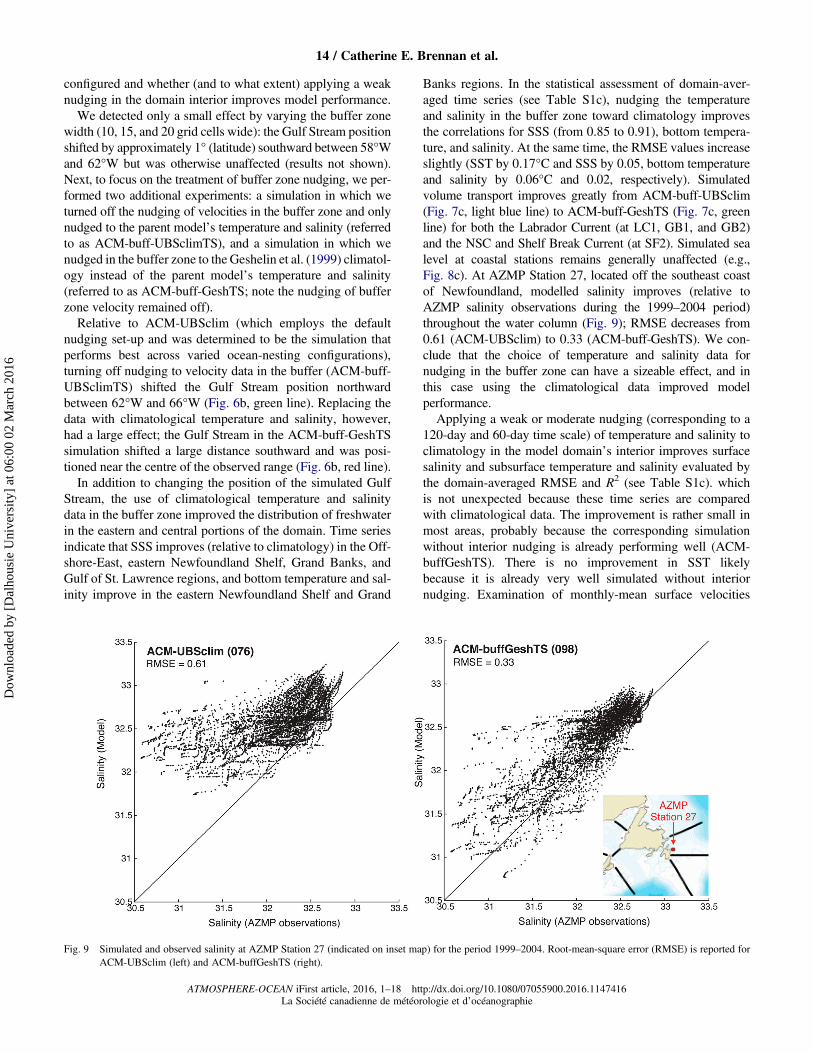
Banks regions. In the statistical assessment of domain-aver-aged time series (see Table S1c), nudging the temperatureand salinity in the buffer zone toward climatology improvesthe correlations for SSS (from 0.85 to 0.91), bottom tempera-ture, and salinity. At the same time, the RMSE values increaseslightly (SST by 0.17°C and SSS by 0.05, bottom temperatureand salinity by 0.06°C and 0.02, respectively). Simulatedvolume transport improves greatly from ACM-buff-UBSclim(Fig. 7c, light blue line) to ACM-buff-GeshTS (Fig. 7c, greenline) for both the Labrador Current (at LC1, GB1, and GB2)and the NSC and Shelf Break Current (at SF2). Simulated sealevel at coastal stations remains generally unaffected (e.g.,Fig. 8c). At AZMP Station 27, located off the southeast coastof Newfoundland, modelled salinity improves (relative toAZMP salinity observations during the 1999–2004 period)throughout the water column (Fig. 9); RMSE decreases from0.61 (ACM-UBSclim) to 0.33 (ACM-buff-GeshTS). We con-clude that the choice of temperature and salinity data fornudging in the buffer zone can have a sizeable effect, and inthis case using the climatological data improved modelperformance.

Applying a weak or moderate nudging (corresponding to a120-day and 60-day time scale) of temperature and salinity toclimatology in the model domain’s interior improves surfacesalinity and subsurface temperature and salinity evaluated bythe domain-averaged RMSE and R2 (see Table S1c). whichis not unexpected because these time series are comparedwith climatological data. The improvement is rather small inmost areas, probably because the corresponding simulationwithout interior nudging is already performing well (ACM-buffGeshTS). There is no improvement in SST likelybecause it is already very well simulated without interiornudging. Examination of monthly-mean surface velocities

Fig. 9 Simulated and observed salinity at AZMP Station 27 (indicated on inset map) for the period 1999–2004. Root-mean-square error (RMSE) is reported forACM-UBSclim (left) and ACM-buffGeshTS (right).

14 / Catherine E. Brennan et al.

ATMOSPHERE-OCEAN iFirst article, 2016, 1–18 http://dx.doi.org/10.1080/07055900.2016.1147416La Société canadienne de météorologie et d’océanographie

Dow

nloa

ded

by [

Dal

hous

ie U

nive

rsity

] at

06:

00 0

2 M

arch

201

6

suggests that interior nudging affects circulation featuresthroughout the domain, especially in the interior of themodel domain. The simulated Halifax section (SF2) volumetransport is improved with the application of interiornudging (Fig. 7c). Moderate interior nudging is associatedwith a slightly weaker Gaspé Current in the Gulf ofSt. Lawrence, weaker outflow through Cabot Strait, and aweaker NSC, but a somewhat enhanced shelf break current,and less Gulf Stream variability (though the Gulf Streammean position and coastal sea levels are essentiallyunchanged, as determined by the GSNW index and tide-gauge analysis (Fig. 8c), respectively). Little to no improve-ment is found in the simulated Labrador Current volume trans-port at LC1 or Flemish Pass (GB1) with the application ofinterior nudging.

7 Model assessment IV: Effect of expanding the modeldomain

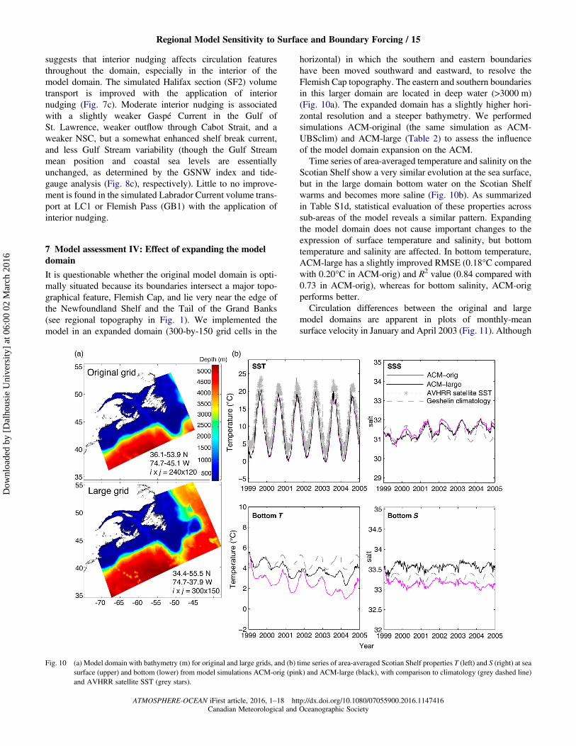
It is questionable whether the original model domain is opti-mally situated because its boundaries intersect a major topo-graphical feature, Flemish Cap, and lie very near the edge ofthe Newfoundland Shelf and the Tail of the Grand Banks(see regional topography in Fig. 1). We implemented themodel in an expanded domain (300-by-150 grid cells in the

horizontal) in which the southern and eastern boundarieshave been moved southward and eastward, to resolve theFlemish Cap topography. The eastern and southern boundariesin this larger domain are located in deep water (>3000 m)(Fig. 10a). The expanded domain has a slightly higher hori-zontal resolution and a steeper bathymetry. We performedsimulations ACM-original (the same simulation as ACM-UBSclim) and ACM-large (Table 2) to assess the influenceof the model domain expansion on the ACM.

Time series of area-averaged temperature and salinity on theScotian Shelf show a very similar evolution at the sea surface,but in the large domain bottom water on the Scotian Shelfwarms and becomes more saline (Fig. 10b). As summarizedin Table S1d, statistical evaluation of these properties acrosssub-areas of the model reveals a similar pattern. Expandingthe model domain does not cause important changes to theexpression of surface temperature and salinity, but bottomtemperature and salinity are affected. In bottom temperature,ACM-large has a slightly improved RMSE (0.18°C comparedwith 0.20°C in ACM-orig) and R2 value (0.84 compared with0.73 in ACM-orig), whereas for bottom salinity, ACM-origperforms better.

Circulation differences between the original and largemodel domains are apparent in plots of monthly-meansurface velocity in January and April 2003 (Fig. 11). Although

Fig. 10 (a) Model domain with bathymetry (m) for original and large grids, and (b) time series of area-averaged Scotian Shelf properties T (left) and S (right) at seasurface (upper) and bottom (lower) from model simulations ACM-orig (pink) and ACM-large (black), with comparison to climatology (grey dashed line)and AVHRR satellite SST (grey stars).

Regional Model Sensitivity to Surface and Boundary Forcing / 15

ATMOSPHERE-OCEAN iFirst article, 2016, 1–18 http://dx.doi.org/10.1080/07055900.2016.1147416Canadian Meteorological and Oceanographic Society

Dow

nloa

ded

by [

Dal

hous

ie U

nive

rsity

] at

06:

00 0

2 M

arch

201

6

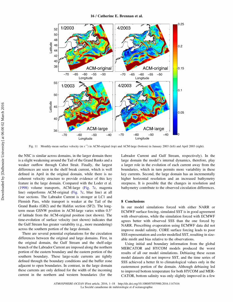
the NSC is similar across domains, in the larger domain thereis a slight weakening around the Tail of the Grand Banks and aweaker outflow through Cabot Strait. Finally, the largestdifferences are seen in the shelf break current, which is welldefined in April in the original domain, while there is nocoherent velocity structure to provide evidence of this keyfeature in the large domain. Compared with the Loder et al.(1998) volume transports, ACM-large (Fig. 7c, magentaline) outperforms ACM-original (Fig. 7c, blue line) at allfour sections. The Labrador Current is stronger at LC1 andFlemish Pass, while transport is weaker at the Tail of theGrand Banks (GB2) and the Halifax section (SF2). The long-term mean GSNW position in ACM-large varies within 0.5°of latitude from the ACM-original position (not shown). Thetime-evolution of surface velocity (not shown) indicates thatthe Gulf Stream has greater variability (e.g., more meandering)across the southern portion of the large domain.There are several potential explanations for the circulation

differences between the original and large domains. First, inthe original domain, the Gulf Stream and the shelf-edgebranch of the Labrador Current are imposed along the northernportion of the eastern boundary and the eastern portion of thesouthern boundary. These large-scale currents are tightlydefined through the boundary conditions and the buffer zoneadjacent to open boundaries. In contrast, in the large domainthese currents are only defined for the width of the incomingcurrent in the northern and western boundaries (for the

Labrador Current and Gulf Stream, respectively). In thelarge domain the model’s internal dynamics, therefore, playa larger role in the evolution of each current away from theboundaries, which in turn permits more variability in thesekey currents. Second, the large domain has an incrementallyhigher horizontal resolution and an increased bathymetrysteepness. It is possible that the changes in resolution andbathymetry contribute to the observed circulation differences.

8 Conclusions

In our model simulations forced with either NARR orECMWF surface forcing, simulated SST is in good agreementwith observations, while the simulation forced with ECMWFagrees better with observed SSS than the one forced byNARR. Prescribing evaporation using ECMWF data did notimprove model salinity. CORE surface forcing leads to poorSSS representation and cooler modelled SST, resulting in size-able misfit and bias relative to the observations.

Using initial and boundary information from the globalMERCATOR and HYCOM models produced the worstresults of all our model simulations. Debiasing these oceanmodel datasets did not improve SST, and the time series ofSSS achieved a better fit to climatological values only in theeasternmost portion of the domain. Although debiasing ledto improved bottom temperature for both HYCOM and MER-CATOR, bottom salinity was only slightly improved in a few

Fig. 11 Monthly-mean surface velocity (m s−1) in ACM-original (top) and ACM-large (bottom) in January 2003 (left) and April 2003 (right).

16 / Catherine E. Brennan et al.

ATMOSPHERE-OCEAN iFirst article, 2016, 1–18 http://dx.doi.org/10.1080/07055900.2016.1147416La Société canadienne de météorologie et d’océanographie

Dow

nloa

ded

by [

Dal

hous

ie U

nive

rsity

] at

06:

00 0

2 M

arch

201

6

regions (in the Grand Banks and eastern Newfoundland Shelffor MERCATOR and in the Offshore regions and the easternNewfoundland Shelf for HYCOM). We conclude that debias-ing (i.e., replacing temperature and salinity monthly-meanvalues with those from climatology) of global ocean parentmodels does not guarantee model improvement.Model simulations employing initial and boundary infor-

mation constructed from the larger scale regional model ofUrrego-Blanco and Sheng (2012; UBS) outperformed simu-lations nested in global ocean parent models. ACM-UBSclim using long-term, monthly-mean UBS data per-formed as well as ACM-UBS and is the preferred simulationbecause of its climatological boundary conditions.Additional sensitivity experiments focused on the treatment

of nudging in the buffer zone adjacent to open boundaries.These experiments revealed that nudging velocities in thebuffer zone was not important in the model but that thechoice of temperature and salinity data had a large effect.By nudging temperature and salinity in the buffer zone to cli-matology instead of UBSclim, the Gulf Stream positionshifted southward to the centre of the observed range, and sal-inity in the eastern portion of the domain was much improved.Applying weak (120-day) or moderate (60-day) nudging in themodel domain interior appeared to improve the distribution oftemperature and salinity further and affected regional currents(improving some features and worsening others).Expanding the model domain to the east and south to

resolve Flemish Cap and increase the distance betweenmodel boundaries and topographical gradients had littleeffect on sea surface properties but had a larger effect on themodel’s bottom level. On the Scotian Shelf, bottom tempera-ture and salinity increased compared with the original domain.Important differences emerged with respect to key circulationfeatures, for example, in the large domain the surfaceexpression of the shelf break current was less evident,coupled with a weaker Cabot Strait outflow, and a more vari-able (meandering) Gulf Stream than in the original domain.This work presents an investigation of the impacts of model

configuration choices on model performance. Perhapsespecially because our regional model is situated in acomplex coastal environment, influenced by large currentsystems from the north (Labrador Current) and the south

(Gulf Stream), model configuration choices can greatlyaffect model results. We assessed 3.5 surface forcing datasets,six ocean model nesting choices, two model grids, and varioustypes of nudging to climatology in the buffer zone and modelinterior for the years 1999–2004. We expect the model iscapable of reproducing other time periods; for example, corre-sponding to different North Atlantic Oscillation states, pro-vided appropriate surface forcing and boundary conditionsare applied, though this has not been investigated in thisstudy. In addition to optimizing our own model’s configur-ation and performance, our results provide useful guidancein model development and testing of other regional oceanmodels, both within the northwest North Atlantic and beyond.

Acknowledgements

We thank Christoph Renkl for his contributions to the prep-aration of surface forcing data and model assessment scripts.We thank Kyoko Ohashi for her advice on the implementationof rivers in the model. We are grateful to Wei Chen for extract-ing the sea level data and performing analyses. We also thankRui Zhang for his assistance in evaluating model currents.

Funding

We acknowledge funding by the Marine EnvironmentalObservation Prediction and Response Network (MEOPAR).

Disclosure statement

No potential conflict of interest was reported by the authors.

Supplemental data

Supplemental data for this article can be accessed at http://dx.doi.org//10.1080/07055900.2016.1147416.

ORCID

Catherine E. Brennan http://orcid.org/0000-0003-2593-7222Laura Bianucci http://orcid.org/0000-0002-4492-8930Katja Fennel http://orcid.org/0000-0003-3170-2331

ReferencesAnderson, C., & Smith, P. C. (1989). Oceanographic observations on theScotian shelf during CASP. Atmosphere-Ocean, 27, 130–156.

Barnier, B., & Ferry, N. (2011). GLobal Ocean Reanalyses and Simulations:GLORYS2V1 product scientific and technical notice for users. Technicalnotice version 1. Mercator-Ocean, Ramonville-Saint-Ange, France.

Barnier, B., Madec, G., Penduff, T., Molines, J.-M., Treguier, A.-M., LeSommer, J.,…De Cuevas, B. (2006). Impact of partial steps and momen-tum advection schemes in a global ocean circulation model at eddypermitting resolution. Ocean Dynamics, 56, 543–567. doi:10.1007/s10236-006-0082-1

Cummings, J. A. (2005). Operational multivariate ocean data assimilation.Quarterly Journal of the RoyalMeteorological Society, 131(613), 3583–3604.

Dee, D. P., Uppala, S. M., Simmons, A. J., Berrisford, P., Poli, P.,Kobayashi, S.,…Vitart, F. (2011). The ERA-Interim reanalysis:Configuration and performance of the data assimilation system.Quarterly Journal of the Royal Meteorological Society, 137, 553–597.doi:10.1002/qj.828

Fairall, C. W., Bradley, E. F., Godfrey, J. S., Wick, G. A., Edson, J. B., &Young, G. S. (1996). Cool-skin and warm-layer effects on sea surface temp-erature. Journal of Geophysical Research, 101, 1295–1308.

Fairall, C. W., Bradley, E. F., Rogers, D. P., Edson, J. B., & Young, G. S.(1996). Bulk parameterization of air-sea fluxes for tropical ocean globalatmosphere coupled-ocean atmosphere response experiment. Journal ofGeophysical Research, 101, 3747–3764.

Regional Model Sensitivity to Surface and Boundary Forcing / 17

ATMOSPHERE-OCEAN iFirst article, 2016, 1–18 http://dx.doi.org/10.1080/07055900.2016.1147416Canadian Meteorological and Oceanographic Society

Dow

nloa

ded

by [

Dal

hous

ie U

nive

rsity

] at

06:

00 0

2 M

arch

201

6

Fisheries and Oceans Canada. (2011). Hydrographic data: Stations and sec-tions of AZMP [Data]. Retrieved from http://www.meds-sdmm.dfo-mpo.gc.ca/isdm-gdsi/azmp-pmza/hydro/index-eng.html

Fisheries and Oceans Canada. (2015). Canadian station inventory and datadownload. Retrieved from http://www.isdm-gdsi.gc.ca/isdm-gdsi/twl-mne/maps-cartes/inventory-inventaire-eng.asp

Geshelin, Y., Sheng, J., & Greatbatch, R. J. (1999). Monthly mean climatolo-gies of temperature and salinity in the western North Atlantic. CanadianData Report of Hydrography and Ocean Sciences, 153, Dartmouth, NovaScotia, Canada: Bedford Institute of Oceanography.

Government of Canada. (2015). Wateroffice: Historical hydrometric datasearch [Data]. Retrieved from the Water Survey of Canada website http://wateroffice.ec.gc.ca/search/search_e.html?sType=h2oArc

Griffies, S. M., Winton, M., & Samuels, B. L. (2004). The Large and Yeager(2004) dataset and CORE. CORE release notes. Retrieved from http://data1.gfdl.noaa.gov/nomads/forms/mom4/CORE/doc.html

Guo, L., Perrie, W., Long, Z., Chassé, J., Zhang, Y., & Huang, A. (2013).Dynamical downscaling over the Gulf of St. Lawrence using the CanadianRegional Climate Model. Atmosphere-Ocean, 51(3), 265–283. doi:10.1080/07055900.2013.798778

Haidvogel, D. B., Arango, H., Budgell, W. P., Cornuelle, B. D., Curchitser, E.,Di Lorenzo, E.,…Wilkin, J. (2008). Regional ocean forecasting in terrain-following coordinates: Model formulation and skill assessment. Journal ofComputational Physics, 227, 3595–3624. doi:10.1016/i.jcp.2007.06.016

Han, G. (2000). Three-dimensional modeling of tidal currents and mixingquantities over the Newfoundland shelf. Journal of GeophysicalResearch, 105, 11407–11422.

Han, G. (2005). Wind-driven barotropic circulation off Newfoundland andLabrador. Continental Shelf Research, 25, 2084–2106. doi:10.1016/j.csr.2005.04.015

Han, G., & Loder, J. W. (2003). Three-dimensional seasonal-mean circulationand hydrography on the eastern Scotian shelf. Journal of GeophysicalResearch, 108, 1–21. doi:10.1029/2002JC001463

Han, G., Lu, Z., Wang, Z., Helbig, J., Chen, N., & de Young, B. (2008)Seasonal variability of the Labrador Current and shelf circulation offNewfoundland. Journal of Geophysical Research, 113, C10013. doi:10.1029/2007JC004376

Joyce, T. M., Deser, C., & Spall, M. A. (2000). The relation between decadalvariability of subtropical model water and the North Atlantic Oscillation.Journal of Climate, 13, 2550–2569.

Kilpatrick, K. A., Podesta, G. P., & Evans, R. (2001). Overview of the NOAA/NASA Advanced Very High Resolution Radiometer Pathfinder algorithmfor sea surface temperature and associated matchup database. Journal ofGeophysical Research: Oceans, 106(C5), 9179–9197.

Large, W. G., & Yeager, S. G. (2004). Diurnal to decadal global forcing forocean and sea-ice models: The data sets and flux climatologies. CGDDivision of the National Center for Atmospheric Research, NCARTechnical Note: NCAR/TN-460+STR. Boulder, CO: NCAR.

Lazier, J. R. N., & Wright, D. G. (1993). Annual variations in the LabradorCurrent. Journal of Physical Oceanography, 23, 659–678.

Liu, W. T., Katsaros, K. B., & Businger, J. A. (1979). Bulk parameterizationof the air-sea exchange of heat and water vapor including the molecular con-straints at the interface. Journal of Atmospheric Science, 36, 1722–1735.

Loder, J. W., Petrie, B., & Gawarkiewicz, G. (1998). The coastal ocean offnortheastern North America: A large-scale view. In A. R. Robinson & K.H. Brink (Eds.), The sea. Vol 11, The global coastal ocean: Regionalstudies and syntheses (pp. 105–133). New York, USA: John Wiley &Sons, Inc.

Marchesiello, P., McWilliams, J. C., & Shchepetkin, A. F. (2001). Openboundary conditions for long-term integration of regional ocean models.Ocean Modelling, 3, 1–20.

Mesinger, F., DiMego, G., Kalnay, E., Mitchell, K., Shafran, P. C., Ebisuzaki,W.,… Shi, W. (2006). North American regional reanalysis. Bulletin of theAmerican Meteorological Society, 87, 343–360. doi:10/1175/BAMS-87-3-343.

Pawlowicz, R. (2011). T_Tide harmonic analysis toolbox. Retrieved fromhttps://www.eoas.ubc.ca/~rich/#T_Tide

Pawlowicz, R., Beardsley, B., & Lentz, S. (2002). Classical tidal harmonicanalysis including error estimates in MATLAB using T_TIDE.Computers and Geosciences, 28, 929–937.

Petrie, B., & Buckley, J. (1996). Transport and freshwater flux of the LabradorCurrent in flemish pass. Journal of Geophysical Research, 101, 28335–28342.

Petrie, B. D., & Drinkwater, K. (1993). Temperature and salinity variability onthe Scotian Shelf and in the Gulf of Maine 1945–1990. Journal ofGeophysical Research, 98, 20079–20089.

Pham, D. T., Verron, J., & Roubaud, M. C. (1998). A singular evolutiveextended Kalman filter for data assimilation in oceanography. Journal ofMarine Systems, 16(3), 323–340.

Therriault, J.-C., Petrie, B., Pepin, P., Gagnon, J., Gregory, D., Helbig, J.,…Sameoto, D. (1998). Proposal for a Northwest Atlantic zonal monitoringprogram. Canadian Technical Report of Hydrography and Ocean Sciences,194. Retrieved from http://www.dfo-mpo.gc.ca/Library/224076.pdf

Thompson, K. R., Loucks, R. H., & Trites, R. W. (1988). Sea surface temp-erature variability in the shelf-slope region of the northwest Atlantic.Atmosphere-Ocean, 26, 292–299.

Tranchant, B., Testut, C.-E., Renault, L., Ferry, N., Birol, F., & Brasseur, P.(2008). Expected impact of the future SMOS and Aquarius Ocean surfacesalinity missions in the Mercator Ocean operational systems: New perspec-tives to monitor the ocean circulation. Remote Sensing of Environment, 112,1476–1487.

Umlauf, L., & Burchard, H. (2003). A generic length-scale equation for geo-physical turbulence models. Journal of Marine Research, 61, 235–265.

Urrego-Blanco, J., & Sheng, J. (2012). Interannual variability of the circula-tion over the eastern Canadian Shelf. Atmosphere-Ocean, 50, 277–300.doi:10.1080/07055900.2012.680430

Warner, J. C., Sherwood, C. R., Arango, H. G., & Signell, R. P. (2005).Performance of four turbulence closure models implemented using ageneric length scale method. Ocean Modelling, 8, 81–113. doi:10.1016/j.ocemod.2003.12.003

Wilkin, J. L., & Hunter, E. J. (2013). An assessment of the skill of real-timemodels of Mid-Atlantic Bight continental shelf circulation. Journal ofGeophysical Research: Oceans, 118, 2919–2933. doi:10.1002/jgrc.20223

Zhang, H., & Sheng, J. (2013). Estimation of extreme sea levels over theeastern continental shelf of North America. Journal of GeophysicalResearch: Oceans, 118, 6253–6273. doi:10.1002/2013JC009160

18 / Catherine E. Brennan et al.

ATMOSPHERE-OCEAN iFirst article, 2016, 1–18 http://dx.doi.org/10.1080/07055900.2016.1147416La Société canadienne de météorologie et d’océanographie

Dow

nloa

ded

by [

Dal

hous

ie U

nive

rsity

] at

06:

00 0

2 M

arch

201

6