SENSOR ARRAY OPTIMIZATION FOR MULTIPLE HARMONIC SOUND ... · for multiple harmonic sound source separation and doa. ... sensor array optimization for multiple harmonic sound ... bss:

Master’s DissertationEngineering

Acoustics

ELISABET SUÁREZ LÓPEZ

SENSOR ARRAY OPTIMIZATION FOR MULTIPLE HARMONIC SOUNDSOURCE SEPARATION AND DOA

Denna sida skall vara tom!

Engineering Acoustics Department of Construction Sciences

Copyright © 2013 by Engineering Acoustics, LTH, Sweden.Printed by Media-Tryck LU, Lund, Sweden, May 2013 (Pl).

For information, address:Division of Engineering Acoustics, LTH, Lund University, Box 118, SE-221 00 Lund, Sweden.

Homepage: http://www.akustik.lth.se

SENSOR ARRAY OPTIMIZATION

FOR MULTIPLE HARMONIC SOUND

SOURCE SEPARATION AND DOA

Master’s Dissertation by

ELISABET SUÁREZ LÓPEZ

Kristian Stålne, PhD,Div. of Structural Mechanics, LTH, Lund

Delphine Bard, PhD, Div. of Engineering Acoustics, LTH, Lund

Supervisor:

Examiner:

ISRN LUTVDG/TVBA--13/5042--SE (1-89)ISSN 0281-8477

Denna sida skall vara tom!

PREFACE

This Master Thesis was carried out at the division of Acoustics Engineering at LTH, Lund University, from September 2012 to April 2013. I would like to thank Delphine Bard, who encouraged me to reach more ambitious goals. Special appreciation to Anders Sjöström for his assistance as well as Juan Negreira for his help and advice. I would also to thank Brüel & Kjær for providing their equipment for making the measurements. Thanks again to my friends in Barcelona and all the people I met during my stay in Sweden, because this experience would not have been carried out without the continuous support of my family, specially my sister Anna.

The scope of this Master Thesis is to design a Goniometer Antenna for sound localization and study the optimal sensor array geometry for sound separation.

Basically, the first part summarizes our research work on how to realize a Goniometer Antenna based on the measurement of the phase delays between two microphones (sensors). Using the properties of the FFT, the delay extraction is done and then the localization on the 2D space is possible.

Otherwise, the second step is about the design of an algorithm able to find the optimal position of the sensors. It takes into account the criterion of minimizing the distance between microphones, and with the goal to separate the different harmonic sound sources in the at-worst case: 2 sensors and 2 sources.

After that, some measurements were carried out in the anechoic chamber. The results obtained in different experiments are presented to verify the algorithms programmed with Matlab.

In the last place, an extension of that work is explained for one extra sound source situation.

ABSTRACT

INTRODUCTION

In the last years a lot of researches about source separation have been realized, like extraction of a signal of interest (vocal recognition application), identification of which source gives which sound (motor engine applications) or noise source characterization (environmental application). Most of these techniques for sound source estimation use the signal-subspace approach, where the number of emitting sources is determined by the multiplicity of the lowest eigenvalue of the correlation matrix. The problems arise when the number of microphones is equal to the number of sources radiating, hence the noise subspace could not exist.

This Master Thesis investigates how to realize a Goniometer Antenna to record communications, as well as the implementation of an algorithm to optimize the location of the sensors with the intend of separating the different sound sources in the at-worst case (number of sources equal number of sensors). It has been achieve using the eigenvalues of the correlation matrix of the received signals and the delay between microphones. Finally, measurements in the anechoic chamber verified the proposed approach.

METHODS

An acoustic goniometer is a system that measures the angle between a source and a receptor using the phase delay, thereby obtaining the source direction. The design dwell on two sensors (microphones) collocated in the 2D space in a concrete geometry. The implementation of each algorithm was done in Matlab based on two parts: the time delay estimation used in source localization by computing the azimuth in [2], and also an adaptation of the MPE block carried out in [4]. Likewise different methods based on the properties of the correlation matrix have been studied for delay estimating like in [3].

Apart from that, in [1] is explored the relation between sensor array geometry and eigenvalues to obtain the optimal sound sources separation and detection. This theory has been put into practice in programming in Matlab: minimization of the distance between microphones such that accomplish the condition of sources separation or sources detection. The optimization procedure has been done using two different SQP Methods: Active Set and Interior Point.

Moreover, an optimization approach is presented for a system composed by two sensors and three sound sources. Several options based on mathematical theory has been considered for solving the problem. Eventually, taking advantage of the procedure followed in [1] and combined with the circumcenter calculation, the optimal distance for the microphones can be found.

RESULTS

Afterwards all this work, different simulations with the code in Matlab were tested reaching successful results. Then, a process of validation is required in the anechoic chamber for more realistic measurements.

CONCLUSIONS

In conclusion is demonstrated by theoretical calculation at first and then by experimental measurements that the optimal array geometry could help to improve the sound source separation approach.

Forthcoming works will consist in extending this work for larger bandwidth and much more sound sources. Also, taking into consideration a more realistic model with reflections, interfering signals or noise corrupted.

PAPERS

This thesis is based on the following papers, which will be referred to in the text by their Roman numerals.

I - Sensor array optimization for sources separation and detection in the at-worst determined case. Patrick Marmaroli, Xavier Falourd, Hervé Lissek. (2011)

II – Multiple harmonic sound sources separation in the under-determined case based on the merging of goniometric and beamforming approach. Patrick Marmaroli, Xavier Falourd, Hervé Lissek. (2009)

III – Acoustic Goniometry Antennas and Algorithms. Eric Van Lancker, Mario Rossi.

IV – Robust Multipitch estimation for the analysis and manipulation of polyphonic musical signals. Anssi Klapuri, Tuomas Virtanen, Jan-Markus Holm.

ABBREVIATIONS AND SYMBOLS

AIC: Akaike Information Criteria

BSS: Blind Source Separation

DOA: Direction of Arrival

ESM: Electronic Surveillance Measure

ESPIRIT: Estimation of Signal Parameters via Rotational Invariance Techniques

FFT: Fast Fourier Transform

FT: Fourier Transform

ICA: Independent Component Analysis

i.i.d. noise: independent identically distributed noise

MDL: Minimum Description Length

MPE: Multipitch Estimator

MUSIC: Multiple Signal Classification

PCA: Principal Components Analysis

PPD: Predominant Pitch Detection

RF: Radio Frequency

SQP: Sequential Quadratic Programming

SVD: Singular Value Optimization

SVM: Support Vector Machines

CONTENTS

1. Introduction and aims of the study 1

2. Theoretical Background 3

2.1 Sound waves 3

2.2 Propagation model 4

2.3 Delay extraction 5

2.3.1 2D geometry: 2 sensors and 1 source 6

2.3.2 2D geometry: 2 sensors and 2 sources 11

2.4 Source separation 15

2.4.1 Subspace approach 16

2.4.2 Subspace approach for the at-worst case 21

2.4.3 Extension 31

3. Experiment and measurements 37

3.1 2D location of a source with 2 sensors 38

3.1.1. Ideal situation with one harmonic 38

3.1.2. Ideal situation with voice pitch 39

3.1.3. Anechoic chamber situation 40

3.1.4. Conclusions 44

3.2 2D locations of two sources with two sensors 44

3.2.1. Ideal situation: two harmonics 45

3.2.2. Anechoic chamber situation 47


3.3 Optimization of two sources separation 50

3.3.1. Description of the devices 50

3.3.2. Procedure 51

3.3.3. Results 53


4. Discussion 57

5. Suggestions for further work 59

Appendix 61

Bibliography 85

1

1. INTRODUCTION AND AIMS OF THE STUDY

Identification and extraction of noise components of a sound source is usually done by acoustic beamformers. Despite these techniques depend on the number of microphones and the a priori knowledge of the sound source location, they are still in use. Hence, there is a need to know the location of the sources.

A goniometer is defined as an instrument that measures angles (displays phase relationships). An acoustic goniometer is therefore a system which measures the direction of arrival (DOA) of sounds, and thus estimates the source direction. A goniometer is made up of an antenna, composed of several sensors arranged in a particular geometry, and a calculation algorithm on Matlab, which carried out the development and implementation, but not in real time.

In fact, there are two different types of goniometers:

Active goniometer: the signal source is under control

Passive goniometer: the location of the sources is unknown. They are also called noise sources.

According to signal processing literature, DOA means the direction from which a wave arise a sensors array. Also, it has usually associated a beamforming technique which estimated the signal from a given direction.

For this reason, DOA has been the object of a large number of researches. Several sensor systems exist in which DOA estimation is present, such as radar, sonar, Electronic Surveillance Measure (ESM), localization applications, Radio telescopes applications (to look at a certain location in the sky), in RF applications as wireless communication, etc.

Because of the wide range of application topics for DOA estimation, a lot of algorithms have been proposed such as Capon [10], Multiple Signal Classification (MUSIC) [10] or Estimation of Signal Parameters via Rotational Invariance Techniques (ESPRIT) [10].

Next step, remains in the interest in source separation owing to the numerous applications. Some examples are:

Noise source characterization in environmental application

Extraction of a signal of interest in vocal recognition application

Music enhancement

Structured coding of audio signals

Identification of which source gives which sound in motor engine application

As a result, different techniques were developed during the last decades in order to achieve the most accurately estimations, such as adaptive beamformers, classical time delay estimations, spatial filtering approach, spectral based methods etc.

2

However, subspace based estimation techniques change the sensor array signal processing literature. The subspace based approach consists on the study of the eigenvalues of the correlation matrix of the received signals. Actually, most of the new techniques for sound source estimation use the signal-subspace approach (Music or Esprit), where the number of emitting sources is determined by the multiplicity of the lowest eigenvalue of the correlation matrix.

In other words, the number of sources N is equal to the number of sensors M minus the number of noise eigenvalues. Based on the suppose that M > N.

The noise eigenvalues are equal in an ideal case and easy to identify. Unfortunately, in a real situation eigenvalues are not exactly equal due to correlation matrix estimation, but they are very close. There exist algorithms to estimate closeness of the eigenvalues that would be the radio of their geometric mean to their arithmetic mean. Based on it can be defined two different information criteria [8]: AIC (Akaike Information Criteria) and MDL (Minimum Description Length).

The problem arises when the number of microphones is equal to the number of sources radiating, hence the noise subspace could not exist. That problematic was solved in [1] optimizing the sensor array for sources separation in the at-worst determined case. Especially attention was made for the situation M=N=2.

Essentially, this Master Thesis was motivated for the increasing need for acoustic localization systems and sources separation using the minimum number of sensors. Optimize the equipment using a technique which has reported good results, is an important improvement to achieve more applications with less effort.

As a matter of fact, the scoop of this work is to design a Goniometer Antenna for sound localization using the properties of the FFT, study the optimal sensor array geometry for sounds separation and finally present an extension for the sound sources separation in the at-worst situation with one extra sound source.

3

2. THEORETICAL BACKGROUND

2.1. SOUND WAVES

The sound is a longitudinal wave (the movement of the particles is perpendicular to the propagation direction) which usually travels in the air. The motion in the air creates pressure changes that human ear could understand as sound. These changes usually are increases and decreases of the pressure following the equation for a pure wave:

(2.1)

Figure 2.1 Example of sound wave

Where:

x(t) : space

t : time

ω = 2πf : angular frequency

A : amplitude (indicates sound volume of the wave)

α : phase (time when the oscillation starts)

λ = v/f : wave length (space ranged by the sound in a cycle)

v = x/t : speed of the wave

4

Sound is propagated at a constant speed although it depends on:

Atmospheric pressure

Temperature

Humidity

Amount of diatomic gases, suspension particles and dust

Sound propagation speed in the air:

(2.2)

Sound propagation speed in the air at 23ºC: c ≈ 345 [m/s]

2.2. PROPAGATION MODEL

For this specific situation, a propagation model has been defined. Far-field propagation has been supposed because it can be considered that the location of the source is far enough, it could be assumed es << r. As a result, planar waves fall on the sensors as shows Figure 2.2.

Figure 2.2 Far-field propagation model.

Planar waves can be understood as a planar surface moving at a concrete velocity in a straight line, so the propagation direction is perpendicular to the wave front. That surface represents all the points with the same pressure level.

5

Figure 2.3 Planar surface moving representing the propagation of a planar wave.

Equation of one-dimensional waves

(2.3)

The solution depends on a constant related with the initial conditions

(2.4)

On the contrary, when the source is located close to the sensors, spherical propagation must be looked upon. In this study, this possibility is not taken into account because far-field scenario is supposed.

2.3. DELAY EXTRACTION

The propagation delay could be defined as the length of time it takes for a signal to travel to its destination. It could be computed as the ratio between the length source-sensor and the propagation speed, in this case, the sound speed c=345 m/s.

(2.5)

6

2.3.1. 2D GEOMETRY: 2 SENSORS AND 1 SOURCE

Firstly, the easiest configuration of two sensors in 2D space was implemented, taking into account the assumption of far-field propagation explained in the previous point.

Knowing the propagation delay between the pair of sensors and the distance d between them it is possible to compute the angle of incidence of the wave’s propagation direction: θ. In Figure 2.4 is possible to appreciate the configuration.

Figure 2.4 2D representation of incidence angle of the wave’s propagation direction θ, propagation delay δ between the pair of sensors and distance d between them.

Applying simple trigonometric calculations and considering Eqn (2.5):

(2.6)

(2.7)

7

DIFFERENT METHODS FOR CALCULATING THE DELAY

METHODS BASED ON THE CROSS-CORRELATION

The signal emitted by the source is a harmonic of frequency f1:

x1(t) = A1 sin (2πf1t) (2.8)

The signals received at each sensor are a delayed version of x1(t) because of the distance of propagation:

yA(t)= A1A x1( t - δA ) = A1A sin ( 2πf1 ( t - δA ) ) (2.9)

yB(t)= A1B x1( t - δB ) = A1B sin ( 2πf1 ( t - δB ) ) (2.10)

The signals received could also be expressed in a way related with the delay between microphones: δ = δA-δB, because of the distance between sensors. And let’s suppose the amplitude is the same A1A = A1B = A.

yA(t) = A x1( t - δA ) (2.11)

yB(t) = A x1( t - δB ) = A x1( t - δA + δA - δB ) = yA( t - δB + δA ) = yA ( t – δ ) (2.12)

(a) (b)

Figure 2.5 (a, b) Representation of signal yA(t) in (a) and signal yB(t) in (b). Both signals of length L=150 samples and frequency sampling FS = 44100. The harmonic frequency f=500 Hz and delay δ=0.68027 ms (corresponding to 30 samples).

In signal processing, the cross-correlation of two waveforms is a measure of similarity between them.

For continuous functions, f and g, the cross-correlation is defined as Eqn (2.13)

8

(2.13)

Where * indicates the complex conjugate.

For discrete functions, the cross-correlation is defined as Eqn (2.14)

(2.14)

(2.15)

One useful application of cross-correlation is the time delay calculation between two signals because of the propagation across a microphone array. Then the maximum (or minimum if the signals are negatively correlated) of the cross-correlation function indicates the point in time where the signals are best aligned.

Compute the cross-correlation between yA(t) and yB(t)

RBA ( τ ) = E { yB(t) · yA( t + τ ) } = E { yA ( t – δ ) · yA( t + τ ) } = RAA ( τ - δ ) (2.16)

Knowing that the auto-correlation of yA(t) looks like Figure 2.6. Notice that the correlations in Matlab are shifted and the origin corresponds to the midpoint in the graph.

Figure 2.6 Representation of signal RAA(τ).

9

The cross-correlation is only a delayed version of RAA(τ) where the maximum now is located in τ = δ.

Figure 2.7 Representation of signal RBA(τ). The maximum correspond to the abscissa 180 which means τ=180-L=30.

Once the cross-correlation peaks have been stored, they each have to be attributed to different sound waves picked up. Thus, the complexity of the problem increases. Also the frequency sampling has to be taken into account in order to compute the delay into the time domain in seconds.

(2.17)

Alternatively, there is another method which computes the Fourier Transform of the cross-correlation:

(2.18)

Consider the phase because it contains the delay information:

(2.19)

10

Hence, the slope of the phase is:

(2.20)

Finally the delay can be calculated as:

(2.21)

This method is much complex because of the phase slope. Since it is not an ideal model, has errors, the results may not be appropriately adjusted to reality.

METHOD BASED ON THE PROPERTIES OF THE FOURIER TRANSFORM

As is known, the Fourier Transform of a signal f(t) is shown in Eqn (2.22)

(2.22)

The first steps applied to the received signal in the previous method, are also followed by, obtaining Eqn (2.12). Then the Fourier Transform of the received signal is computed:

(2.23)

(2.24)

11

With the change u = t-τ:

(2.25)

(2.26)

The delay can be found:

(2.27)

And the delay corresponding to the harmonic signal emitted is found evaluating Eqn (2.27) at the desired frequency: ω1 = 2πf1.

Obviously, the technique based on the Fourier Transform properties is much more efficient when there are several sources emitting, thus it will be useful regarding the purpose of the whole project. So in the next sections the delay extraction will be done using this method.

2.3.2. 2D GEOMETRY: 2 SENSORS AND 2 SOURCES

Let’s consider a situation with two sources emitting and our array composed by two microphones separated a distance d, like shows Figure (2.8)

The study is done with the assumption of mutually uncorrelated harmonic sound sources which each one emits a sinusoid of different frequency (f1 and f2). Also independent identically distributed noise (i.i.d. noise) is used.

12

Figure 2.8 2D representation a system of 2 sources and 2 sensors separated a distance d.

The signals emitted by the sources are presented in Eqn (2.28) and (2.29).

x1(t) = A1 sin (2πf1t) (2.28)

x2(t) = A2 sin (2πf2t) (2.29)

Consequently, each sensor (A and B) receives a delayed version of each one:

yA(t) = x1( t - δA1 ) + x2( t – δA2) = yA1(t) + yA2(t) (2.30)

yB(t) = x1( t - δB1 ) + x2( t - δB2 ) = yB1(t) + yB2(t) (2.31)

Figure 2.9 2D representation of incidence angle of the wave’s propagation direction θ for a system of 2 sources and 2 sensors separated a distance d.

13

The purpose is still the computation of the delay between yA1(t) and yB1(t), and between yA2(t) and yB2(t). So it means that every delay it’s related with a different frequency, thus the first block should detect which are those frequencies: it will be done with an iterative estimation and separation approach to Multipitch Estimation (MPE). And then the delay extraction and angle extraction will follow as is shown in Figure 2.10.

Figure 2.10 Localization system in 2D space composed by MPE Block, Delay Extraction Block and Angle Extraction Block.

Now every block is going to be described in more detail:

BLOCK FREQUENCY EXTRACTION (MPE)

A typical MPE (as in [4]) is composed by a three blocks:

Predominant Pitch Detection: Recognize the different frequencies corresponding to each source. It is necessary to compute the FFT of the input signal and then detect the picks of the FFT (search the maximum).

Estimation of the sound spectrum

Remove partials: Remove the estimated frequencies from the spectrum.

And this procedure is iterated as many times as number of sources are on (see Figure 2.11)

Figure 2.11 Typical Block MPE composed by PPD, Estimate sound spectrum and Remove partials.

14

In our application, estimation of sound spectrum is not compulsory, because there is no need to know the shape of the signal, just the location of the picks of the FFT in order to extract the harmonic frequencies. For that reason the MPE block has been simplified eliminating the Estimation Sound Spectrum block as indicated in Figure 2.12.

Figure 2.12 Block Frequency extraction: MPE composed by PPD and Remove Block.

BLOCK DELAY EXTRACTION

As it was discussed previously, the delay extraction is implemented with the use of the FFT properties. Then, the function defined in Eqn (2.27) evaluated at each frequency ω1 and ω2, outcome each delay (in milliseconds) between the signal from source 1 arriving to sensor A and B (delay 1), and the same with the signal from source 2 (delay 2).

Figure 2.13 Block Delay extraction.

BLOCK ANGLE EXTRACTION (localization in 2D)

As it was done in the simplest case of only one source, the process of localization gives the angles θ1 and θ2 that indicated the direction of the sources in the 2D space using Eqn (2.5).

15

Figure 2.14 Block Angle extraction (localization in 2D).

Eventually, the whole system composed by the three blocks described previously, is displayed in Figure 2.15.

Figure 2.15 2D localization blocks diagram: Frequency, Delay and angle extraction.

2.4. SOURCE SEPARATION

The second part of this Master Thesis deals with the problem of sound source separation. The sound source separation deals with the following problem: given a set of mixed signals, the goal is to separate the set of source signals without the knowledge of information about the source signals or the mixing process. Thus the problem is highly underdetermined.

Figure 2.16 Illustrative diagram of signal separation problem.

16

This is usually known as Blind Source Separation (BSS) in the signal processing literature. The main field of application is in signal audio, although it has being adopted in video and image restoration during the last years.

There exist different methods of blind signal separation:

Principal components analysis (PCA)

Singular value decomposition (SVD)

Independent component analysis (ICA)

Dependent component analysis

Non-negative matrix factorization

Low-complexity coding and decoding

Stationary subspace analysis

Common spatial pattern

Even though there exist a considerable amount of techniques and literature concerning BSS, in this Master Thesis is going to be focused only on SVD-based methods ([1] and [10]).

2.4.1. SUBSPACE APPROACH

Now the purpose is to achieve an estimation of the signal and noise subspace employing a subspace approach. This technique is based on the SVD (Singular Value Decomposition) of the correlation matrix and the study of its eigenvalues and eigenvectors.

SVD in linear algebra is a factorization of a mxn real or complex matrix of the form

M = U Σ V* (2.32)

Where U is a mxm unitary matrix

Σ is a rectangular diagonal matrix with nonnegative real numbers on the diagonal

V* (conjugate transpose of V) is an nxn unitary matrix

The diagonal of Σ are the singular values of M (σ). The non-zero singular values of M are the square roots of the non-zero eigenvalues of both M*M and MM*.

The m columns of U are the left-singular vectors of M (u).

The n columns of V are the right-singular vectors of M (v).

Mv=σu and M*u=σv (2.33)

http://en.wikipedia.org/wiki/Principal_components_analysis

http://en.wikipedia.org/wiki/Singular_value_decomposition

http://en.wikipedia.org/wiki/Independent_component_analysis

http://en.wikipedia.org/w/index.php?title=Dependent_component_analysis&action=edit&redlink=1

http://en.wikipedia.org/wiki/Non-negative_matrix_factorization

http://en.wikipedia.org/w/index.php?title=Low-complexity_coding_and_decoding&action=edit&redlink=1

http://en.wikipedia.org/wiki/Stationary_subspace_analysis

http://en.wikipedia.org/wiki/Common_spatial_pattern

17

A typical application of the SVD is that provides an explicit representation of the range of M. The left-singular vectors (u) corresponding to the non-zero singular values (σ) of M span the range of M. As a consequence, the rank of M equals the number of non-zero singular values which is the same as the number of non-zero diagonal elements in Σ.

PROPOSAL OF THE GENERAL CASE

Let’s suppose a general case:

The array consists of M omnidirectional sensors mi located in xmi ϵ R2 where 1 ≤ i ≤ M

NMAX is the number of maximum mutually independent and isotropic sources

N is the number of sources radiating, 0 ≤ N ≤ NMAX

Each source sj is located in xsj ϵ R2 and its wavelength is λj and amplitude is βj,

where 1 ≤ j ≤ NMAX

Figure 2.17 General case diagram: NMAX sources and M sensors.

It is possible to build a signal processing system:

X = A · S + W (2.34)

X is a vector of the M signals received at the array

A is a matrix MxN which contains the attenuations and delays on time of the source signals

S is a vector of the N source signals on

W is a vector noise (i.i.d.)

(2.35)

18

SVD DESCOMPOSITION

Taking into consideration the SVD technique, described above, focusing in the last part of range calculation, the rank of R could be deduced:

If there is supposed that no ambiguity appears (two sources symmetrically located respect to the array) each component of X vector, xi, is a linear combination of the source signals sj and the coefficient of attenuation and delay aij, and they are independent. Thus the rank of the correlation matrix R is equal to N (number of sources on). [Appendix 1]

R = E { X · XH } = A · Ψ · AH + σ2 I (2.36)

Ψ is the signal correlation matrix

σ2 Id is the noise correlation matrix MxM

rank { R } = rank { A · Ψ · AH + σ2 I } = N (2.37)

The structure of the correlation matrix, defined positive, could be studied in terms of eigenvalues and eigenvectors:

(2.38)

Where E= [ e1, e2, … , eN, eN+1, eN+2, … , eM ] (2.39)

and satisfies R · ei = Λi · ei (2.40)

As said before, the rank of the correlation matrix R is equal to N. Consequently, estimate the number of sources is equivalent to estimate the rank of R. That means that the next step is a study of the M eigenvalues of R:

Λi = μi + σ2 with 1 ≤ i ≤ N and μi ϵ R+ (2.41)

Λi = σ2 with N+1 ≤ i ≤ M (2.42)

19

Figure 2.18 General case of M eigenvalues, where N correspond to signal subspace and M-N correspond to noise subspace (assuming M>N).

In the case of M > N every eigenvector ei associated to each eigenvalue Λi can be separated in two groups (see Figure 2.18):

Signal subspace which is associated to the highest N eigenvalues:

ES = [ e1, e2, … , eN ] (2.43)

Noise subspace which is associated to the lowest M - N eigenvalues:

EN = [ eN+1, eN+2, … , eM ] (2.44)

DIFFERENT METHODS OF SUBSPACE APPROACH FOR ESTIMATING THE NUMBER OF SOURCES

METHOD 1: BASED ON THE MULTIPLICITY OF THE NOISE EIGENVALUE

Using subspace based approach, actually, the number of emitting sources is determined by the multiplicity of the lowest eigenvalue of the correlation matrix. The lowest eigenvalues of the correlation matrix correspond to the noise.

ΛN+1 = ΛN+2 = … = ΛM = σ2 (2.45)

Hence, knowing the number of sensors M, minus the number of noise eigenvalues, we obtain the number of sources N. Obviously based on the suppose that M > N.

# sensors - # noise eigenvalues = # sources (2.46)

20

Unfortunately, the noise eigenvalues are only equal in an ideal case. In a real situation, those eigenvalues are not exactly equal due to correlation matrix estimation and also the noise level is time-variant, so they are not easy to identify. Nevertheless, they are very close.

There exist several algorithms to estimate the number of sources:

a. Support vector machines (SVM)[7]

Using SVM and maximum likelihood adaptive beamformer number of sources could be estimated. It doesn’t need pre-whitening or precise estimation of the background noise level.

b. Estimators based on Information Theoretic Criteria (ITC) [8]

There exist algorithms to estimate closeness of the eigenvalues that would be the radio of their geometric mean to their arithmetic mean. Based on it can be defined two different information criteria:

AIC (Akaike Information Criteria)

MDL (Minimum Description Length).

METHOD 2: MULTIPLE SIGNAL DESCOMPOSITION (MUSIC)

One of the most important methods of SVD is MUSIC [10]. This procedure is based on the properties of the eigenvalues and the eigenvectors of the correlation matrix. It has good resolution but is poor in reliability.

For describing and explaining the characteristics of this method, the same reasoning has been followed as in [10].

Looking at Eqn (2.37), the dimension of the signal space N, can be obtained through the rank of the diagonal matrix Ψ, or through the power of the sources.

The signal subspace is expanded through the vectors of the matrix A which are not orthonormal. If the signal subspace has dimension N, it means that M-N eigenvectors don’t contribute to that space.

If the eigenvectors which describe the space build by the directions contained in A, are denominated as signal eigenvectors, it is clear that the rest of the eigenvectors will be orthogonal to all of them. Hence, they will be also orthogonal to all the sources in the scenario.

In conclusion, the zeros of the M-N noise eigenvectors have to appear where the sources are present.

In other words, if the noise eigenvectors don’t have projection in the signal subspace, then it will be verified:

AH · ei = 0 with i= N+1, … , M (2.47)

21

That’s why it is easy to check that all of its eigenvalues are equal to the noise level.

R · ei = σ2 · ei with i= N+1, … , M (2.48)

For the same reason, the signal eigenvalues will be always superior to the noise level. All of them are positive because of the covariance matrix is defined positive.

Notice that from the calculation of the eigenvectors of the matrix, the number of sources N present in the scenario will be obtained; or maybe, the number of elements in the array, M, minus the number of eigenvalues equal to the minimum, included it, give the number of sources.

Another more efficient way, in terms of quality in the estimation of the position, is calculating the zeros of the polynomial that results from the scalar product of the direction vector and the eigenvector. Anyway, this method, called “Root-Music” is complicated for the case of no uniform or planar apertures.

In Music, the problem of determining the dimension of the signal subspace has its origin, for the 2 sources case, in which the first eigenvalue grows with the power of both sources but the second decreases with its proximity. In other words, when we detect two sources in the scenario, the closer they are, the more difficult it results. Moreover, if one of them gets weaker than the other the decision gets harder in terms of estimating the number of sources. As said before, a resolution barrier is found in that problem.

2.4.2. SUBSPACE APPROACH FOR THE AT-WORST CASE

Despite the fact that those techniques report acceptable results, they just can be useful when the number of sources is less than the dimension of the array (N<M). Therefore, the problem arises when the number of microphones is equal at the number of sources radiating: M = N. Hence the noise subspace could not exist, and another solution must be looked for.

Figure 2.19 Case of M=N eigenvalues which corresponds to signal subspace (noise subspace could not exist).

22

OPTIMIZATION METHOD FOR THE CASE M=NMAX=2

Taking into account the subspace theory studied, if the at-worst case is considered (number of sensors and sources on is the same) is clearly that noise subspace could not exist.

Figure 2.20 At-worst case: M=N=2. The signal subspace dimension is 2, thus noise subspace could not exist.

According to Eqn (2.35), the system is shown in Eqn (2.49)

(2.49)

Matrix A contains the information about sensors, as well as, sources locations and its wavelengths.

(2.50)

Hence, the matrix system is modified like in Eqn (2.51)

(2.51)

23

where its parameters are presented in the group of equations Eqn (2.52).

(2.52)

Considering the far-field propagation model described in previous sections, the distance between sensors is lower than the distance source-sensor. Hence, the coefficients of the matrix A can be simplified: γij = αj where αj is a positive constant that represent the initial intensity level of the source j.

As a consequence, matrix A changes its parameters:

(2.53)

Take for granted that the sources are mutually uncorrelated and i.i.d noise, then:

rank{ R } = rank{ E{ A·AH } } (2.54)

If Λ is an eigenvalue of A·AH, it will satisfy Eqn (2.40). As a result:

det( A·AH - Λ ·I ) = 0 (2.55)

Solving Eqn (2.55) as shown in Appendix 2, the eigenvalues can be found:

(2.56)

24

(2.57)

(2.58)

SOURCE SEPARATION CONTEXT

In source separation context, the main goal to achieve is the separation of two sound signals emitted by two different sources, when are received by two microphones (see the previous Figure 2.16). In order to obtain the best result (in terms of source separation), the optimal array geometry is being seek. Now the situation looks like this Figure (2.21)

Figure 2.21 Representation of a general situation in source separation

Knowing:

- Location of the microphone 1: xm1

- Location of the sources 1 and 2: xs1 and xs2

- Source frequencies: f1 and f2

Find:

Optimal location of the microphone 2 (xm2) allowing a geometric multiplicity of A·AH equal to the maximum number of sources (NMAX).

find xm2 such that dim[ Ker( A · AH - Λ I ) ] = NMAX (2.59)

25

Consider the theory about algebraic and geometric multiplicity in Appendix 3.

In the case of NMAX = 2, the characteristic polynomial is

p(Λ) = det (A · AH - Λ · I ) = (Λ – Λ 1 ) · (Λ – Λ 2 ) (2.60)

and the geometric multiclicity:

mi = dim[ Ker( A · AH - Λ · I ) ] (2.61)

If it is desired to have algebraic and geometric multiplicity equal to the maximum number of sources, NMAX = 2, then:

Λ1 = Λ2 (2.62)

Eqn (2.62) implies:

(2.63)

Starting to solve it:

(2.64)

Then,

(2.65)

So, it must fulfill the condition:

(2.66)

If k·α1 = α2 then the condition Eqn (2.66) changes to 1 + k2 ≤ 2 k (2.67)

If k = 1 the optimal xm2 can be found where source 1 and 2 have the same initial radiating intensity (α1 = α2). So taking into account Eqn (2.65) it results:

26

(2.68)

The substitution of the values of a, b, c and d, defined in Eqn (2.52), ends in a function of xm2 defined by Eqn (2.69):

(2.69)

SOURCE DETECTION CONTEXT

In source detection context, the purpose is to detect the number of sources which are emitting. In the case of NMAX = 2, when the number of sources needs to be estimated, three different situations can occur:

1. Two sources radiate

2. One source radiates

3. No sources radiate

The value of α1 and α2 are not known, hence the eigenvalues Λ1 and Λ2 are difficult to predict. To make it easier a ratio r = Λ2 / Λ1 is considered.

In the case 1:

If h( xm2 ) = 0 k=1 Δ = 0 Λ1 = Λ2 r=1

In the case 3:

If i.i.d. noise X=W R= σ2 I Λ1 = Λ2 = σ2 r=1

So, when r = 1 the cases 1 and 3 can’t be dissociated. Another optimal xm2 has to be found to avoid r = 0 and r = 1.

In the case 2, considering Eqn (2.41) and (2.42)

Λ1 = μ1 + σ2 and Λ2 = σ2 (2.70)

27

Assuming μ1 >> σ2:

r = Λ2 / Λ1 = σ2 / ( μ1 + σ2 ) ≈ 0 (2.71)

Let’s suppose we are working in the case 1, and to avoid ambiguity 0 < r < 1

Following the mathematical procedure appended in Appendix 4, it is concluded:

if α1 = α2 (k=1) choose xm2 such that a – b – c +d ≠ ± 0.5 (2.72)

if α1 ≠ α2 (k≠1) choose xm2 such that a – b – c +d ≠ Z

Now given a value of k and r it can established a condition for a, b, c and d, as well as finding the optimal value of xm2. In Appendix 5 there is the mathematical procedure followed in order to obtain a function of xm2 with the parameters r and k. As a result Eqn (2.73) is presented.

(2.73)

OPTIMIZATION CRITERIA

To find the optimal position of the microphone 2 we can use the criteria of minimizing the distance between the pair of microphones:

(2.74)

Subject to the constraint found in the previous parts Eqn (2.69) or Eqn (2.73)

In other words:

find xm2 є R2 such that minimize f (xm2 ) subject to h(xm2) = 0 (2.75)

28

Now is necessary to solve a nonlinear convex optimization problem. The best option is using a Local-SQP Method (Sequential Quadratic Programming) because we are in front of a problem of quadratic constrained quadratic programming situation.

PROGRAMMED CODE

SQP is an iterative method for nonlinear optimization that is used on problems for which the objective function and the constraints are twice continuously differentiable, so SQP solve a sequence of optimization problems.

According to the previous work, the optimization block was also done in Matlab language. The use of a predefined function called ‘fmincon’, able to find the minimum of constrained nonlinear multivariable function, facilitate the implementation of the code programed. Two methods were tested, Active-Set method and Interior-Point method, both with approximately the same effectively.

Hence, the global system will be composed by two blocks: MPE and Optimization (see Figure 2.22). The first one will provide the frequencies of the harmonics and the second block will optimize the position of xm2 for sources separation with the desired purpose or method.

Figure 2.22 Diagram of Optimization for sources separation

PROGRAMMED CODE TESTING

Before starting to do some measurements in the laboratory, is preferable to check if the results obtained in a hypothetical situation are reasonable. That’s why three different cases were examined to test the programmed code in Matlab.

29

CASE 1

Let’s consider two sound sources S1 and S2 each radiates a harmonic sound of the frequency f1 = 3 kHz and f2 = 1 kHz, and with the same level of intensity (k=1). The position of the sources is xS1 = (0, 0) and xS2 = (0.5, 0). The position of the fixed microphone is xm1 = (0, -2).

Then applying the algorithm is possible to find the optimal position of the second microphone:

Separation method: xm2 = ( 0.9143, -1.7417 )

Detection method: xm2 = ( 0.9063, -1.7250 )

Figure 2.23 Optimization case 1

CASE 2

Let’s consider two sound sources SA and SB each radiates a harmonic sound of the frequency fA = 3 kHz and fB = 2 kHz, and with the same level of intensity (k=1). The position of the sources is xA = (0, 0) and xB = (0.5, 0). The position of the fixed microphone is x1 = (0, -3).


Separation method: x2 = ( 1.2725, -2.3769 )

Detection method: x2 = ( 1.2587, -2.3415 )

30


CASE 3

Let’s consider two sound sources SA and SB each radiates a harmonic sound of the frequency fA = 700 Hz and fB = 500 Hz, and with the same level of intensity (k=1). The position of the sources is xA = (0, 0) and xB = (0.5, 0). The position of the fixed microphone is x1 = (0, -3).


Separation method: x2 = ( 1.4867, -2.9148 )

Detection method: x2 = ( 1.4311, -2.7235 )


31

2.4.3. EXTENSION

Furthermore, an extension with one source more has been implemented and the problem increases its complexity.

Let’s suppose we have N = 3 sources and we know its locations: xs1, xs2 and xs3; and its wavelengths: λ1, λ2 and λ3. Assume we have only M = 2 sensors, and one of them is fixed xm1 and the other we want to find the optimal position xm2 in order to achieve sound source separation.

Figure 2.26 Optimization general case: 3 sources and 2 sensors

Now the system still looks like Eqn (2.34). But notice that now the matrix A is not square because has different dimensions: 2x3.

(2.76)

So the previous solution based on the eigenvalues of a 2x2 matrix is not useful.

As an alternative an algorithm was designed based on the previous work done for two sources and two sensors:

Random measurement with the fixed microphone to recognize f1, f2 and f3, corresponding to the frequencies of the three sources xS1, xS2 and xS3.

Obtain xm2_12opt: optimal position of microphone 2 considering only sources 1 and 2



32

Calculate the optimal position of the second sensor (consider all sources): x M2opt

Iterate or do it another time to fix the parameters or improve the results (optional)

The way to carry out the calculation of x M2opt could be done in different ways. We have

studied 2 options: Fermat Point and Circumcenter.

FERMAT POINT

The 3 points xm2_12opt, xm2_13

opt and xm2_23opt compose a triangle. In geometry, the Fermat

point of a triangle or also called Torricelli point fulfils that the sum of the distances from the vertices of the triangle to the point (AF + BF + CF), is minimum (See Figure 2.18).

Figure 2.27 Fermat Point F corresponding to the triangle composed by A, B and C.

CIRCUMCENTER

Given a set of points { p1, p2, p3 } in the Euclidian Space, pk is a point corresponding to Voronoi cell Rk. Every point accomplish that the distance to pk is less than or equal to its distance to any other side. Each cell is obtained from the intersection of half-spaces and hence, it’s a convex polygon.

33

Figure 2.28 Example of how to achieve Voronoi regions.

Figure 2.29 Example of the result of Voronoi decomposition.

The circumcenter C is the point of intersection of the three perpendicular bisectors of the sides (see Figure 2.30). It’s the center of the circumcircle of the triangle and also the three vertices { A, B, D } are at the same distance to C.

Figure 2.30 Example of circumcenter of a triangle.

34

But if one of the angles of the triangle measures more than 120º, then the circumcenter will appear outside the closed region which forms the three points. Hence the best option in those situations is computing the midpoint of the longest side of the triangle.

As a result, the solving procedure has the following steps:

1. Measure the sides of the triangle

2. Compute the angles

3. Check if any angle is more than 90º. If it is compute circumcenter as the midpoint of the longest side. If not, go to step 4.

4. Compute midpoint of each side of the triangle.

5. Calculate slopes of the sides.

6. Compute slopes of the perpendicular bisectors.

7. Generate the equations of the perpendicular bisectors.

8. Find coordinated of the circumcenter by solving any 2 of the 3 above equations.

It has decided to implement the circumcenter method in order to optimize the sensor array geometry for the case of three sound sources separation.

Optimization of sound source separation (three sources)

Let’s consider three sources located in the 2D space emitting at different frequencies:

xs1 = (0,0) f1 = 2000 Hz x1(t) = sin (2πf1 t) (2.77)

xs2 = (0.5,0) f2 = 3000 Hz x2(t) = sin (2πf2 t) (2.78)

xs3 = (0.35,0.2) f3 = 1000 Hz x3(t) = sin (2πf3 t) (2.79)

Those signals delayed are recorded by a microphone located in xm1 = (0,-4) m. Apply the algorithm described above (Matlab code in Appendix 6: test_Voronoi.m). The options chose is Active set method for sound source separation and parameters k=1 and r=1.

The optimal position of the second microphone corresponds to the circumcenter:

xm2 = (0.0364,-4.0084)

35

It can be found because of the three optimal locations found by choosing different pair of sources:

xm2_12 = (0.0585,-3.8460)

xm2_13 = (0.0142,-4.1708)

xm2_23 = (-0.0125,-4.0853)

Figure 2.31 Optimization case: 3 sources and 2 sensors (Example)

37

3. EXPERIMENT AND MEASUREMENTS

Every study has a part where the theoretical must be demonstrated in real cases. Hence, a process of validation is required for the algorithms programmed.

- 2D location: 1 sound source with 2 sensors

- 2D location: 2 sound sources with 2 sensors

- Optimization for sources separation: 2 sound sources with 2 sensors

Firstly, some simulations of ideal cases are presented for each approach in different situations.

Secondly, more realistic situations were implemented in the anechoic chamber. The measurements were carried out in November 2012 and January 2013 at the Department of Acoustics.

Lastly, the results are analyzed and commented in a short conclusion.

Anechoic chamber

An anechoic chamber is a room designed to absorb the sound that reaches the walls, ceiling and floor, in order to reduce the sound reflection. It is covered with blocks of fiberglass or foams to absorb the sound and increase the dispersion of the unabsorbed sound, thus it can avoid the effects of the echo and sound reverberation.

(a) (b)

Figure 3.1 Different examples of anechoic chambers.

38

3.1. 2D LOCATION OF A SOURCE WITH TWO SENSORS

Localize the position of one sound source emitting a harmonic signal at frequency f using the delay δ between a pair of microphones.

Figure 3.2 2D representation of incidence angle of the wave’s propagation direction θ, propagation delay δ between the pair of sensors and distance d between them.

3.1.1. IDEAL SITUATION WITH ONE HARMONIC

Suppose a sound source emitting a harmonic of frequency f=500 Hz:

x(t) = sin(2π f t) (3.1)

Which a delayed version reaches the sensors:

xA(t) = x(t) = sin(2π f t) (3.2)

xB(t) = x(t-δ) = x(t-·10-4) = sin(2π f (t-·10-4)) (3.3)

Because of the frequency sampling (Fs=44100) in discrete:

xA[n] = x[n] = sin(2π f n) (3.4)

xB[n] = x[n-45] = sin(2π f (n-45)) (3.5)

It is supposed a separation between sensors: d= 0.5 m. Compute the frequency, delay δ and the angle θ using two different methods:

- Method 1: Cross-correlation (code in Appendix 6: test1.m)

- Method 2: Properties FT (code in Appendix 6: test2.m)

The results are presented in the Table 3.1

39

Table 3.1 Error in angle extraction for a simulation with method 1 (cross-correlation) and method 2 (FT Properties).

Method 1 Method 2 Real

f 499.6376 Hz 500 Hz δ 1.0204 ms 0.9810 ms 1.0204 ms θ 44.7554º 42.6012º 44.7554º

|Eθ| 0º 2.1542º

3.1.2. IDEAL SITUATION WITH VOICE PITCH

A human voice was recorded and compared with a 7 samples delayed version. In terms of time, it means a delay δ= 0.875 ms because the frequency sampling is Fs= 8000. Length of the signal is 122149 samples.

Using the Cross-correlation method and the code in Appendix 6: test3.m, the results are presented in Table 3.2.

Table 3.2 Dependence of the distance between microphones and the angle measured θ for a delay δ=0.875 ms.

Distance between microphones θmeas

40 cm 48.9981º 50 cm 37.1389º 60 cm 30.2070º 70 cm 25.5469º 80 cm 22.1692º 90 cm 19.5979º 100 cm 17.5703º

Figure 3.3 Graphic of the dependence of the distance between microphones and the angle measured θ for a delay δ=0.875 ms.

0º

10º

20º

30º

40º

50º

60º

30 50 70 90 110

θmeas

Distance between microphones (cm)

40

It is demonstrated that for the same delay but different distances between microphones (so different array geometry) the location of the source (θ) will be different. Because of the relation between distance and θ showed in Eqn (2.6)

3.1.3. ANECHOIC CHAMBER SITUATION

The devices were connected as shown Figure 3.2 in order to effectuate the measures.

Figure 3.4 Diagram of the measurements carried out in the anechoic chamber with two microphones and one sound source to extract the angle θ.

Description of the devices

Microphones

A pair of Microphones Unit Type 4189-A-021 (Brüel & Kjær)

Figure 3.5 Microphone Unit Type 4189-A-021.

41

3050-a-060

The 3050-A-060 (from Brüel & Kjær) was designed to cover as many sound and vibration measurement application as possible. This module was used for measurements front-end module, it has six high-precision input channels with an input range from DC to 51.2 kHz.

Figure 3.6 3050-A-060.

Cisco SG300-10Mp

The SG300-10Mp model belongs to the Cisco 300 Series which is a portfolio of switches that provides a reliable foundation for network, and also, helps to create a more efficient and better connected workspace.

Figure 3.7 Cisco SG300-10Mp.

Software: Pulse Labshop

The Software employed for data acquisition was Pulse Labshop from Brüel & Kjær. Is one of the most efficient and software used for data acquisition from more than one channel. And it’s equipped to perform fundamental analysis software tasks, the standard Pulse Labshop tools are:

FFT analysis

CPB real-time 1/n octave analysis

Order analysis

42

Envelope analysis

Cepstrum analysis

SSR analysis

Figure 3.8 Examples of Pulse Labshop interfaces for different simulations and measurements

Procedure

The procedure followed for carrying out the measurements consisted on the pair of microphones in a fixed position and doing seven different measurements changing the speaker’s position at the room as indicates the Figure 3.9.

Figure 3.9 Distribution of speaker and microphone sin the anechoic chamber for measurements

The distance between microphones is d = 0.5 m and the distance between each position is ℓ = 1.5 m.

43

Through the software a low signal of length t= 10 s was send to the speaker using the switch and the 3050-A-060 with a high component of ambient noise. Then two recordings were performed with the pair of microphones.

Finally, the use of Pulse LabShop was determinant to complete the data acquisition to save it as a .wav file.

The laboratory work was examined with Matlab. The fragments of data recorded were used as input parameters to compute the δmeas (ms) and the θmeas to localize the sound source in the 2D space.

Results

The results obtained with the cross-correlation method are presented in the Table 3.3. The testing code is in Appendix 6: test4.m.

Table 3.3 Error in angle extraction in the anechoic chamber using cross-correlation method for a system of one source and two microphones.

Position δmeas (ms) θmeas δreal (ms) θreal |Εθ|

1 -1.4286 80.3037º -1.4493 90º 9.6963º 2 -1.0431 46.0320º -1.0248 45º 1.032º 3 -0.6576 26.9840º -0.6481 26.565º 0.419º 4 0.0227 0.8965º 0 0º 0.8965º 5 0.7029 29.0147º 0.6481 26.565º 2.4497º 6 -110.6349 - 1.0248 45º - 7 1.4286 80.3037º 1.4493 90º 9.6963º

Frequency sampling was Fs=44100, hence the signal length L=441000 samples.

The results obtained with the FT method are presented in the Table 3.4. The testing code is in Appendix 6: test5.m.

Table 3.4 Error in angle extraction in the anechoic chamber using FT properties method for a system of one source and two microphones.

Position fmeas δmeas (ms) θmeas δreal (ms) θreal

1 6.4404 kHz 0.0369 1.4596º 1.4493 90º 2 6.4404 kHz 0.0616 2.4341º 1.0248 45º 3 30.1970 Hz -0.7322 -30.3444º 0.6481 26.565º 4 30.9540 Hz -6.1959 - 0 0º 5 40.3748 Hz 0.4818 19.4150º 0.6481 26.565º 6 10.946 Hz 0.0358 1.4139º 1.0248 45º 7 6.4404 kHz 0.0278 1.1003º 1.4493 90º

44

3.1.4. CONCLUSIONS

Overall, using Cross-correlation method the angle error has a strong relation with the relative location of source and sensors, so it means that the error depends on the angle θ as shown in the Figure 3.10.

Figure 3.10 Error angle obtained using cross-correlation in the anechoic chamber.

Above all the results, sources located in the broadside direction (frontal direction: θ = 0º) are better than the case when the source is located in the end-fire region (lateral direction: θ = 90º), because in the end-fire direction the antenna is more sensitive to errors.

However, using the method based on the properties of Fourier Transform there are no conclusive results. The reason is because too much environmental noise was brought into the recordings. Hence, it could wind up that this method is less robust to noise. The critical stage is the MPE because the frequency to detect is masked by the noise level.

3.2. 2D LOCATION OF TWO SOURCES WITH TWO SENSORS

Localize the position of two sources emitting harmonics at different frequencies f1 and f2 using the method based on the FT properties.

0º

1º

2º

3º

4º

5º

6º

7º

8º

9º

10º

-90º -40º 10º 60º

θreal

|Εθ|

45

Figure 3.11 2D representation of incidence angle of the wave’s propagation direction θ for a system of 2 sources and 2 sensors separated a distance d.

3.2.1. IDEAL SITUATION: TWO HARMONICS

Now the number of sources has increased, although, the aim is still the same: compute the frequencies, delays and angles. Besides, the two sinusoidal signals have different frequencies, in this concrete case f1 = 50Hz and f2 = 200 Hz:

x1(t) = sin(2π f1 t) (3.6)

x2(t) = sin(2π f2 t) (3.7)

Which a delayed version reaches the sensors:

xA(t) = x1(t) + x2(t) = sin(2π f1 t) + sin(2π f2 t) (3.8)

xB(t) = x1(t-δ1) + x2(t-δ2) = sin(2π f1 (t-2.875·10-4 )) + sin(2π f2 (t-1.4·10-3 )) (3.9)

Figure 3.12 Representation of xA(t) and xB(t).

46

Because of the frequency sampling (Fs=80000) in discrete domain:

xA[n] = x1[n] + x2[n] = sin(2π f1 n) + sin(2π f2 n) (3.10)

xB[n] = x1[n-23] + x2[n-112] = sin(2π f1 (n-23)) + sin(2π f2 (n-112)) (3.11)

And the length signals is L=100000.

Testing the code is in Appendix 6: test6.m and supposing that the sensors are separated d= 0.5 m the results are:

f1meas = 49.4385 Hz f1real = 50 Hz

f2meas = 199.5850 Hz f2real = 200 Hz

δ1meas = 0.2882 ms δ1real = 0.2875 ms

δ2meas = 1.3965 ms δ2real = 1.4 ms

Computing the FT, could be checked the frequency value of each harmonic (see Figure 3.13)

Figure 3.13 Representation of the FT of xA(t) and xB(t).

With the use of the formula defined in Eqn (2.6) the angles are found:

θ1meas = 11.4702º θ2meas = 74.4963º

θ1real = 11.4419º θ2real = 75.0164º

Thus, the errors in the angles measured are:

|Eθ1|= 0.0283º |Eθ2|= 0.5211º

47

3.2.2. ANECHOIC CHAMBER SITUATION

The verification in the laboratory using the anechoic chamber is exhibit in Figure 3.14, whilst the experiment implementation (devices and procedure) and the verification code in Appendix 6: test7.m. Finally, the results are presented in the Tables 3.5 and 3.6.

Figure 3.14 Representation of angles θ1 and θ2 in the measurements carried out in the anechoic chamber with two microphones and two sound sources for angle extraction.

In order to try to obtain the most realistic results, the angle extracted by the approach has been compared with the mid-point between microphones.

Table 3.5 Error in angle extraction θ1 in the anechoic chamber using FT properties method for a system of two source and two microphones. The parameters are: s (cm), f1 (kHz), δ1 (ms), θ1 (º) and |Eθ1| (º).

s f1meas δ1 meas θ1 meas θ1 real mid-point |E1 mid-point|

15 3.0001 0.0334 4.4048º 1.4321º 2.9727º

23 3.0001 0.0437 3.7585º 2.1953º 1.5632º

30 2.9999 0.0782 5.1609º 2.8624º 2.2985º

38 2.9999 0.1082 5.6373º 3.6239º 2.0134º

45 3.0001 0.1478 6.5058º 4.2892º 2.2166º

53 3.0001 0.0641 2.2907º 5.0480º 2.7573º

60 2.9999 0.1012 3.3348º 5.7106º 2.3758º

68 3.0001 0.0312 0.9059º 6.4659º 5.5600º

82 3.0001 0.0836 2.0150º 7.7822º 5.7672º

98 3.0001 0.1128 2.2759º 9.2764º 7.0005º

48

Figure 3.15 Representation of the angle error θ1 and its dependence on the distance between sensors.

Table 3.6 Error in angle extraction θ2 in the anechoic chamber using FT properties method for a system of two source and two microphones. The parameters are: s (cm), f2 (kHz), δ2 (ms), θ2 (º) and |Eθ2| (º).

s f2 meas δ2 meas θ2 meas θ2 real mid-point |E2 mid-point|

15 1.9999 0.0360 4.7523º 8.0632º 3.3109º

23 1.9999 0.0521 4.4826º 7.3130º 2.8304º

30 1.9999 0.0604 3.9811º 6.6544º 2.6733º

38 2.0001 0.0723 3.7633º 5.8996º 2.1363º

45 1.9999 0.0654 2.8721º 5.2375º 2.3654º

53 1.9999 0.1424 5.3203º 4.4790º 0.8413º

60 1.9999 0.0492 1.6217º 3.8141º 2.1924º

68 2.0001 0.0494 1.4351º 3.0529º 1.6178º

82 1.9999 0.0236 0.5685º 1.7184º 1.1499º

98 2.0001 0.0758 1.5287º 0.1910º 1.3377º

Figure 3.16 Representation of the angle error θ2 and its dependence on the distance between sensors.

0º

1º

2º

3º

4º

5º

6º

7º

8º

10 20 30 40 50 60 70 80 90 100

Distance between sensors (cm)

|Error in θ1|

0º

1º

1º

2º

2º

3º

3º

4º

10 20 30 40 50 60 70 80 90 100


|Error in θ2|

49

3.2.3. CONCLUSIONS

In the simulated situation the results are almost perfect, the errors are quite negligible. However, in a real situation, the errors are more significant. The accuracy of the results obtained depends on different parameters:

The frequency emitted by the sources: f1 and f2.

The frequency sampling: Fs.

The distance between microphones: d.

The distance between sources: ds.

The distance microphone-source: dms.

Considering dms > d and dms > ds because of the application of far-field model propagation.

Taking notice of the error |Eθ|, it is deduced that the perfect situation becomes when d≈ds but d<ds. Hence the location of close sources could be detected with more precision. Actually when d≈ds but d>ds there is an increase of the error because of the geometry of the problem.

When d > ds the computation of the angle θ do not fit exactly with its real value. Because for a high value of d, if the sources are close, it is more difficult to distinguish their location. It occurs the same in the opposite situation, when d is low. The error of localizing a far source increases.

Notice that the sound frequency estimation done bye the MPE block is almost perfect.

3.3. OPTIMIZATION OF TWO SOURCES SEPARATION

The purpose of this experiment is to verify if exist an optimal array geometry which could improve source separation and detection. So, given two speakers emitting at different frequencies, several distances between microphones are tested. Then, the ratio defined as r = Λ2 / Λ1 is computed in order to study the best array geometry for source separation and detection.

Firstly, let’s describe the devices connection. The circuit build for this experiment is the same as the previous one. Figure 3.18 shows it. However, as said before, the purpose has changed: finding optimal position of sensors to achieve the best sources separation.

50

Figure 3.18 Diagram of the measurements carried out in the anechoic chamber with two microphones and two sound sources to optimize the position of microphone 2.

3.3.1. DESCRIPTION OF THE DEVICES

Notice that some devices are the same as the previous measurements so they are not going to be described: microphones, Cisco Switchers and Pulse Labshop.

Function generator

The Rigol DG4062 is two channel function waveform generator to create high quality signals up to 60 MHz.

Figure 3.19 Function Generator: Rigol DG4062

Amplifiers

It is necessarily to amplify the signal coming from the function generator, to give it to the speakers, because they need more input power to work properly. Two models were used:

Sentec acm 1

Sentec monopower amplifier PA9

51

Figure 3.20 Sentec Amplifier

Speakers

JPW Monitor speakers – Audio electronics

Figure 3.21 JPW Monitor speakers

3.3.2. PROCEDURE

The experiment consists in recording the same signals emitted by two speakers separated 50 centimeters, with a pair of microphones varying its position. The purpose is to verify that optimal array geometry is possible and important in sound source separation.

Let’s consider two sound sources S1 and S1. Each radiates a harmonic sound at the frequency f1 = 3 kHz and f2 = 2 kHz, and with the same level of intensity (k=1). The frequency was set with the function generator and the amplitude was fixed at the same level with the amplifiers and also with the function generator.

The position of the sources is xS1 = (0, 0) and xS2 = (0.5, 0). The position of the fixed microphone is xM1 = (0, -3) and the initial position of the variable microphone is xM2 = (0.15, -3), where the abscissa component will be changing.

52

Figure 3.22 Optimization case: 2 sources and 2 microphones

(a) (b)

(c)

53

(d)

Figure 3.23 Devices distribution in the anechoic chamber for optimizing sources separation

The measurement procedure followed was the same as before: with the use of Pulse Labshop two different records of approximately 10 seconds were saved (each one corresponding to each microphone). Since, the position of the second sensor was modified and the same measurements were done.

3.3.3. RESULTS

The measurements have been done for different values of s, where s, in this case, means the distance between microphones. In Appendix 6: eval_experiment.m there is the code testing.

Figure 3.24 Representation of the relation between ratio r and distance between sensors

0

0,1

0,2

0,3

0,4

0,5

0,6

0,7

0,8

0,9

1

10 30 50 70 90 110 130 150 170


r = Λ2 / Λ1 Measured

Theoretical

54

Table 3.7 Measured and Theoretical value of ratio r for different position of microphone 2.

Position Distance (in cm) Value of r

1 15 0.0613 2 23 0.1658 3 30 0.3287 4 38 0.6604 5 45 0.8315 6 53 0.3944 7 60 0.1764 8 68 0.0426 9 75 0.0008 10 82 0.0242 11 90 0.1491 12 105 0.9893 13 120 0.1267 14 138 0.0462 15 153 0.6851 16 170 0.1084

Then applying the algorithm (Appendix 6: test_optim.m) is possible to find the optimal position of the second microphone:

Active set Method

Separation method: x2 = (0.4287, -3) r=1

Detection method: x2 = (0.3475, -3) r=0.5

Interior Point Method

Separation method: x2 = (0.4287, -3) r=1

Detection method: x2 = (0.3475, -3) r=0.5

3.3.4. CONCLUSIONS

It is possible to optimize the array geometry in order to achieve better results for sound source separation and detection.

Clearly the best position for sound sources separation is number 5 where r=0.8315, however the optimal one appears between positions 4 and 5, then the maximal independence between signals recorded is presented.

It is difficult to achieve that result in the case of two microphones, because the first eigenvalue grows with the initial intensity of both sources and the second eigenvalues decreases when the sources get closer.

55

By contrast, the optimal position for r=0.5 (with the minimum distance between microphones) in the sources detection application appears between positions 3 and 4.

Imagine a hypothetically situation of two sources randomly radiating during a concrete period of time. For sources detection there will appear three cases:

(i) No sources radiating: r=1 (Λ1 = Λ2) (ii) One source radiating: r=0 (Λ1 >> Λ2) (iii) Both sources radiating: 0 < r < 1 (Λ1 > Λ2)

So in (iii) the most probable value expected will be r=0.5.

In conclusion, achieving optimal microphone array in the source separation context doesn’t imply optimal source detection geometry, and vice-versa.

57

4. DISCUSSION

Several methods for delay extraction were considered but the same conclusive argument appears independently the method employed: using an array designed for DOA applications implies a variable reliability which depends on the desired angle to be detected.

In other words, sources located in the broadside direction (frontal: θ = 0º) are easier to detect than sources located in the end-fire direction (lateral: θ = 90º). The reason is because the antennas are more sensitive to errors in the end-fire direction than in the broadside.

Focusing on the technique chosen for delay extraction, the one based on MPE block and FFT properties, it gives more advantages in order to compute the azimuth corresponding to the locating sources:

The design is easier

It does not increase the complexity when the number of sources gets higher

Better to adapt with the second system (optimization for source separation and detection)

Also, it has disadvantages, because the results obtained depends on different parameters like the frequency emitted by the sources, the frequency sampling and all the different distances between microphones and sources. The best result arise when d≈ds, considering d<ds, then the location of sources could be detected with more precision.

Hence, the errors in the measurements should not be ignored, and it could be concluded that this system offers the chance to be improved for applications with no ideal conditions (real situations) and for every direction of arrival, geometry and frequencies, in order to reduce the error and make it homogenous independently to the location of the sources and microphones.

Regarding to the optimal array geometry for source separation and detection, some conclusion based on theoretical calculations has been achieved.

The best situation in source separation context come out when the same value for both

eigenvalues (Λ1 = Λ2) is obtained. Unfortunately, it is difficult to achieve that result in the case of two microphones, because the first eigenvalue grows with the initial intensity of both sources and the second eigenvalues decreases when the sources get closer.

Additionally, it has been shown the independence between the optimal geometry for an application of sound source separation, compared with an application for sound source detection. Talking about a detection context, the best value for the ratio is 0.5 (without previous knowledge of initial source intensity) because the three cases should be distinguished easier: 2 sources radiating (r=0.5), 1 source radiating (r=0) and no-sources on (r=1).

In other words, optimal microphone array in source separation context doesn’t imply optimal source detection geometry, and vice-versa.

58

Moreover, an extension with one source more has been implemented. This time, the previous solution based on the eigenvalues of the correlation matrix is not possible because of the dimensions of the matrix. On the other hand, two alternative algorithms were studied. One of them was presented as an improvement of sound source separation in a situation where the number of source exceeds the number of sensors: the circumcenter method. The results are in accordance with sound source separation optimizing sensor array geometry.

To sum up, it has been demonstrated that array geometry has an important role in sound source separation approach, sound source detection approach, and also DOA applications (better broadside direction with d≈ds, but d<ds). Furthermore, a simple but efficient technique for optimizing the array geometry when there is one source extra has been presented.

59

5. SUGGESTIONS FOR FURTHER WORK

As previously stated, this Master Thesis pretends to optimize the number of sensors to detect the maximum number of sources. Obviously, forthcoming works will consist in designing an algorithm for a higher number of sound sources.

Moreover, 3D space should be investigated. At least 4 sensors are needed to handle the localization of the source in a 3D space (tetrahedral cube), but maybe also this system could be optimized for sound source separation in the 3D space.

Reflections with obstacles should be considered, as well as new interfering signals. This would rise in a model that fits much closer to reality, because often, the influence of acoustic interference origins significant deteriorations or even erroneous results.

Likewise, some modifications or improvements could be done in order to reduce the noise. Even so, it has been assumed that noise and signal are not correlated; hence a study in the case of signal corrupted with correlated or colored noise could be considered.

Devices errors should be taken into account; usually measures do not affect significantly to the results obtained, but could mean an improvement in the quality of the system.

Extending this work for larger bandwidth opens also another avenue of investigation. Working with a broadband system implies a different behavior.

61

APPENDIX 1

SVD

By definition:

R = E { X · XH } = E { (A · S + W) · (A · S + W)H }

Applying Hermitical properties:

R = E { (A · S + W) · (SH · AH + WH)}

Hence,

R = E { A · S · SH · AH } + E { W · SH · AH } + E { A · S · WH } + E { W · WH }

Signal and noise are uncorrelated:

E { W · SH · AH } = E { A · S · WH } = 0

Finally,

R = A · E { S · SH } · AH + E { W · WH } = A · Ψ · AH + σ2 I

62

APPENDIX 2

Procedure to solve Eqn (2.43)

Starting from: det( A·AH - Λ ·I ) = 0

Solve the determinant:

Applying trigonometric properties it can be simplified:

Solving the second order equation 2 solutions are obtained:

In a short way:

63

APPENDIX 3

Algebraic and geometric multiplicity

A · AH is a matix N x N with eigenvalues Λi.

ni is the algebraic multiplicity: multiplicity of the root of the characteristic polynomial.

mi is the geometric multiplicity: dimension of the eigenspace which is associated to the eigenvalue Λi . Also understood as: the number of linearly independent eigenvectors which are associated to that eigenvalue. Or even, dimension of the subspace of vectors x for which A · AH · x = Λ · x.

It is satisfied that:

1≤ ni ≤ N

1≤ mi ≤ N

mi ≤ ni

The characteristic polynomial is p(Λ) = det (A · AH - Λ · I )

and when Λ is an eigenvalue: p(Λ) = 0

64

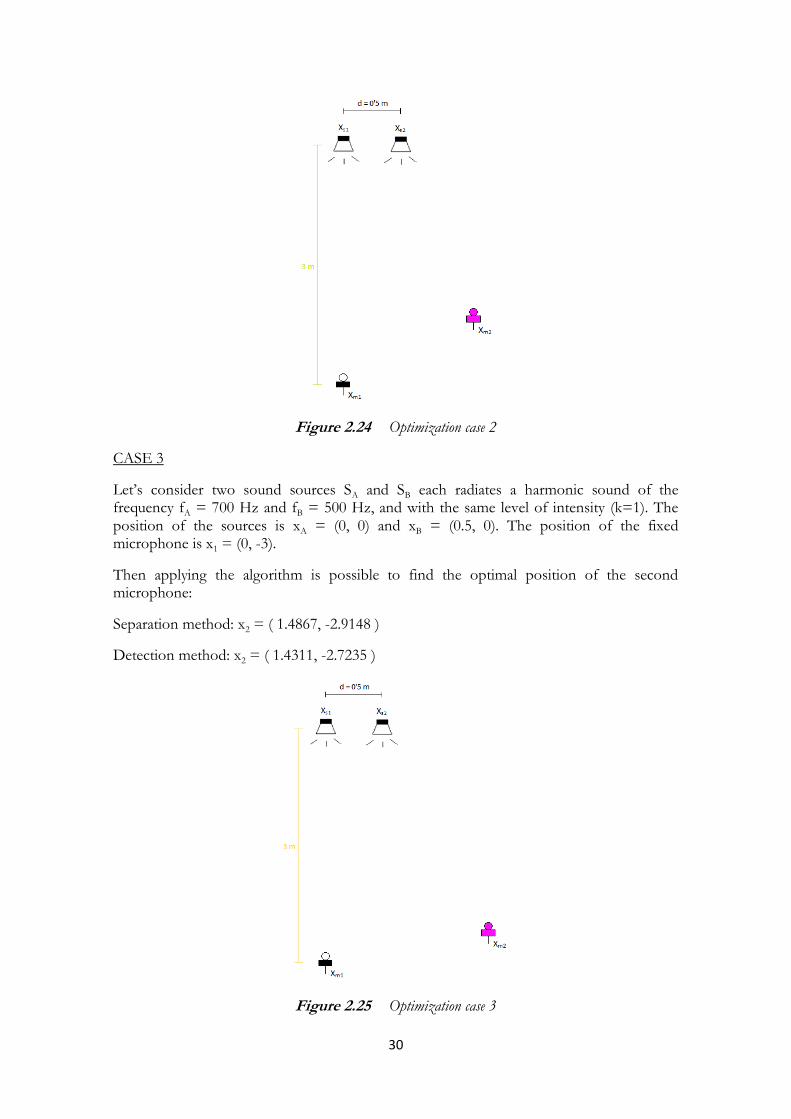
APPENDIX 4

Optimization for sources detection

Starting from :

Assume that both sources are on (case 1)

Case α1 = α2 :

If Δ=0, then r=1, so:

If 2α = Δ, then r=0, so:

Case α1 ≠ α2 :

65

If r=0, then:

If α1 = 0 and α2 ≠ 0, case 2.

If α2 = 0 and α1 ≠ 0, case 2.

If α1 = α2 = 0, case 3.

The last option is:

If r=1, then Δ=0:

If α1 = α2 = 0, case 3.

The last option is:

Eventually, it can be concluded that:

if α1 = α2 (k=1) choose xm2 such that a – b – c +d ≠ ± 0.5

if α1 ≠ α2 (k≠1) choose xm2 such that a – b – c +d ≠ Z

66

APPENDIX 5

Finding the expression Eqn (2.57)

Knowing that:

Replacing in the previous equation of the ratio r:

Try to isolate the term a+d-b-c:

Finally it could be achieve:

67

APPENDIX 6

test1.m

function [angle,delay,Fs] = test1()

d=0.5; % distance between microphones

% produces 2 signals of f=500 Hz delayed 45 samples= 1.0204 ms [x,y,Fs]=block_signals1();

[delay,Rs,Max] = block_delay1(Fs,x,y); %extract the delay

[angle] = block_angle1(delay, d); %extract the angle

end

test2.m

function [frequencies,delay,angle] = test2() N_sources=1; d=0.5; [X,Y,NFFT,Fs]=block_FT(); [frequencies]=block_MPE(X,Y,N_sources,NFFT,Fs); [delay]=block_delay2(X,Y,N_sources,frequencies,Fs,NFFT); [angle]=block_angle2(delay, d);

end

test3.m


d=[0.4 0.5 0.6 0.7 0.8 0.9 1]; angle=zeros(length(d),1);

[x,Fs,nbits]=wavread('grabacion.wav');

y=zeros(length(x),1); % 7 samples delayed version of x for i=1:1:(length(x)-7) y(7+i)=x(i); end

[delay,Rs,Max] = block_delay1(Fs,x,y);

68

for i=1:1:length(d) [angle(i)] = block_angle1(delay, d(i)); end

end

test4.m


d=0.5; % distance between microphones

[x,y,Fs]=block_wavread(); %read signals

[delay,Rs,Max] = block_delay1(Fs,x,y); % compute delay in ms

[angle] = block_angle1(delay, d); %compute angle in degrees

end

test5.m

function [frequencies,delay,angle] = test5()

N_sources=1; %only one source d=0.5; %distance between microphones

[X,Y,NFFT,Fs]=block_wavreadFT(); %read signals and implement FFT

[frequencies]=block_MPE(X,Y,N_sources,NFFT,Fs); %Localize freq

[delay]=block_delay2(X,Y,N_sources,frequencies,Fs,NFFT); % delay

[angle]=block_angle2(delay, d); %compute angle

end

test6.m

function [frequencies,delay,angle] = test6()

N_sources=2; %number of sources d=0.5; %distance between microphones

69

[X,Y,NFFT,Fs]=block_FT2(); % FFT

[frequencies]=block_MPE(X,Y,N_sources,NFFT,Fs); % frequencies

[delay]=block_delay2(X,Y,N_sources,frequencies,Fs,NFFT); % delays

[angle] = block_angle2(delay, d); %compute angles

end

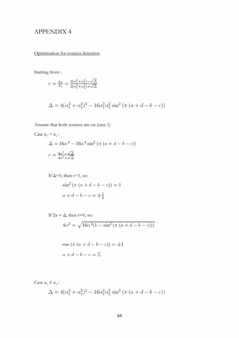
test7.m

function [frequencies,delay,angle] = test7(d)

% d (in m)= distance between microphones, in this case, % abcisa microphone 2: xm2 = (d, -3)

N_sources=2; % 2 sources

[X,Y,NFFT,Fs]=block_wavreadFT(); %FFT

[frequencies]=block_MPE(X,Y,N_sources,NFFT,Fs); % frequencies

[delay]=block_delay2(X,Y,N_sources,frequencies,Fs,NFFT); %delays

[angle] = block_angle2(delay, d); %angles

end

test_Voronoi.m

function [Cc,x12,x13,x23]=

test_Voronoi(method,frequencies,xs1,xs2,xs3,xm1,k,r)

% method= 1: Active set - separation % method= 2: Interior point - separation % method= 3: Active set - detection % method= 4: Interior point - detection

[x_as_separation12, x_ip_separation12, x_as_detection12,

x_ip_detection12] =

test_sources2(frequencies(1),frequencies(2),xs1,xs2,xm1,r,k); [x_as_separation13, x_ip_separation13, x_as_detection13,

x_ip_detection13] =

test_sources2(frequencies(1),frequencies(3),xs1,xs3,xm1,r,k); [x_as_separation23, x_ip_separation23, x_as_detection23,

x_ip_detection23] =

test_sources2(frequencies(2),frequencies(3),xs2,xs3,xm1,r,k);

70

switch method case 1 x12=x_as_separation12; x13=x_as_separation13; x23=x_as_separation23; case 2 x12=x_ip_separation12; x13=x_ip_separation13; x23=x_ip_separation23; case 3 x12=x_as_detection12; x13=x_as_detection13; x23=x_as_detection23; case 4 x12=x_ip_detection12; x13=x_ip_detection13; x23=x_ip_detection23; otherwise disp('Unknown method') return; end

test_optim.m

function [f1,f2,x_as_separation, x_ip_separation, x_as_detection,

x_ip_detection,r] = test_optim()

N_sources=2;

[X,Y,NFFT,Fs]=block_wavreadFT();

[frequencies]=block_MPE(X,Y,N_sources,NFFT,Fs);

f1=frequencies(1); f2=frequencies(2);

xs1= [0,0]; xs2= [0.5,0]; xm1= [0,-3]; xm22=-3; r= 0.5; k= 1;

[x_as_separation, x_ip_separation, x_as_detection, x_ip_detection] =

test_sources1(f1,f2,xs1,xs2,xm1,xm22,r,k);

end

71

test_optim2.m

function [x_as_separation, x_ip_separation, x_as_detection,

x_ip_detection] = test_optim2()

N_sources=2;




xs1= [0,0]; xs2= [0.5,0]; xm1= [0,-3];

r= 0.5; k= 1;

[x_as_separation, x_ip_separation, x_as_detection, x_ip_detection] =

test_sources2(f1,f2,xs1,xs2,xm1,r,k);

end

test_sources1.m


x_ip_detection] = test_sources1(f1,f2,xs1,xs2,xm1,xm22,r,k)

% x_as_separation = Position µphone 2: Active set method, Separation

Condition % x_ip_separation = Position µphone 2: Interior Point method,

Separation Condition % x_as_detection = Position µphone 2: Active set method, Detection

Condition % x_ip_detection = Position µphone 2: Interior Point method, Detection

Condition

x0=0; % Initial point to start

% METHODS

% Define Parameters First

% Positions xm11= xm1(1); % Microphone 1 xm12= xm1(2);

xs11= xs1(1); % Source 1 xs12= xs1(2);

72

xs21= xs2(1); % Source 2 xs22= xs2(2);

% Active set

options = optimset('Algorithm','active-set');

[x_as_detection,fval] =

fmincon(@(xm21)myfun(xm1,xm22,xm21),x0,[],[],[],[],[],[],@(xm21)condit

ion_detection(f1,f2,xs1,xs2,xm1,xm22,xm21,r,k),options); [x_as_separation,fval] =


ion_separation(f1,f2,xs1,xs2,xm1,xm22,xm21),options);

% Interior Point

options = optimset('Algorithm','interior-point');

[x_ip_detection,fval] =


ion_detection(f1,f2,xs1,xs2,xm1,xm22,xm21,r,k),options); [x_ip_separation,fval] =


ion_separation(f1,f2,xs1,xs2,xm1,xm22,xm21),options);

end

test_sources2.m


x_ip_detection] = test_sources2(f1,f2,xs1,xs2,xm1,r,k)

% x_as_separation = Position µphone 2: Active set method, Separation

Condition % x_ip_separation = Position µphone 2: Interior Point method,

Separation Condition % x_as_detection = Position µphone 2: Active set method, Detection

Condition % x_ip_detection = Position µphone 2: Interior Point method, Detection

Condition

x0=[0,0]; % Initial point to start

% METHODS

% Active set

options = optimset('Algorithm','active-set');

[x_as_detection,fval] =

fmincon(@(xm2)myfun2(xm1,xm2),x0,[],[],[],[],[],[],@(xm2)condition_det

ection2(f1,f2,xs1,xs2,xm1,xm2,k,r),options); [x_as_separation,fval] =

fmincon(@(xm2)myfun2(xm1,xm2),x0,[],[],[],[],[],[],@(xm2)condition_sep

aration2(f1,f2,xs1,xs2,xm1,xm2),options);

73

% Interior Point

options = optimset('Algorithm','interior-point');

[x_ip_detection,fval] =

fmincon(@(xm2)myfun2(xm1,xm2),x0,[],[],[],[],[],[],@(xm2)condition_det

ection2(f1,f2,xs1,xs2,xm1,xm2,k,r),options); [x_ip_separation,fval] =

fmincon(@(xm2)myfun2(xm1,xm2),x0,[],[],[],[],[],[],@(xm2)condition_sep

aration2(f1,f2,xs1,xs2,xm1,xm2),options);

end

myfun.m

function f = myfun(xm1,xm22,xm21)

% xm2 = [xm21,-4] position microphone 2

xm11=xm1(1); % xm1 = [0,-4] position microphone 1 xm12=xm1(2);

f= sqrt((xm11-xm21)^2 + (xm12-xm22)^2); % f = norm (xm2-xm1);

end

myfun2.m

function f = myfun2(xm1,xm2)

% xm2 = position microphone 2 % xm1= [0,-3]; % xm1 = position microphone 1

f = norm (xm2-xm1); % norma ~ distance

end

eval_experiment.m

function [r] = eval_experiment(xm2)

% xm2 = position microphone 2

% DEFINITION OF CONSTANTS

74

N_sources=2;




% Positions xm1= [0,-3]; % Microphone 1 xs1= [0,0]; % Source 1 xs2= [0.5,0]; % Source 2

% COMPUTATION OF CONSTANTS

c0=345; % Velocity sound

lamda1= c0/f1; % wavelengths lamda2= c0/f2;

h = (1/lamda1)*(-norm(xm2-xs1) + norm(xm1-xs1)) + (1/lamda2)*(-

norm(xm1-xs2) + norm(xm2-xs2)); % -h=c-a+b-d

B= sin(pi*h); A=sqrt( 1-(B^2)); r = (1-A) / (1+A) ;

end

condition_detection.m

function [c, ceq] =

condition_detection(f1,f2,xs1,xs2,xm1,xm22,xm21,r,k)

% xm21 = abscissa of position microphone 2



xs11= xs1(1); % Source 1 xs12= xs1(2);

xs21= xs2(1); % Source 2 xs22= xs2(2);

% xm22= -3; % Microphone 2

if (k^2 - 2*k +1)>0 disp('ERROR: invalid value of k'); % not valid k

75

return; else




% CONSTRAINTS

% Nonlinear inequality constraints

c = [];

% Nonlinear equality constraints

A= sqrt((xm21-xs11)^2 + (xm22-xs12)^2); %norm(xm2-xs1) B= sqrt((xm11-xs11)^2 + (xm12-xs12)^2); %norm(xm1-xs1) C= sqrt((xm11-xs21)^2 + (xm12-xs22)^2); %norm(xm1-xs2) D= sqrt((xm21-xs21)^2 + (xm22-xs22)^2); %norm(xm2-xs2)

ceq = [(1/lamda1)*(A - B) + (1/lamda2)*(C - D) -

(1/pi)*asin(((1+(k^2))*sqrt(r))/(k*(1+r)))];

end

condition_detection2.m

function [c, ceq] = condition_detection2(f1,f2,xs1,xs2,xm1,xm2,k,r)

if (k^2 - 2*k +1)>0 disp('ERROR: invalid value of k'); % not valid k return; else




% CONSTRAINTS


c = [];


76

ceq = [(1/lamda1)*(norm(xm2-xs1) - norm(xm1-xs1)) +

(1/lamda2)*(norm(xm1-xs2) - norm(xm2-xs2)) -

(1/pi)*asin(((1+(k^2))*sqrt(r))/(k*(1+r)))];

end

condition_separation.m

function [c, ceq] = condition_separation(f1,f2,xs1,xs2,xm1,xm22,xm21)

% xm21 = abcisa of position microphone 2



xs11= xs1(1); % Source 1 xs12= xs1(2);

xs21= xs2(1); % Source 2 xs22= xs2(2);

% xm22= -3; % Microphone 2




% CONSTRAINTS


c = [];


A= sqrt((xm21-xs11)^2 + (xm22-xs12)^2); %norm(xm2-xs1) B= sqrt((xm11-xs11)^2 + (xm12-xs12)^2); %norm(xm1-xs1) C= sqrt((xm11-xs21)^2 + (xm12-xs22)^2); %norm(xm1-xs2) D= sqrt((xm21-xs21)^2 + (xm22-xs22)^2); %norm(xm2-xs2)

ceq = [(1/lamda1)*(A - B) + (1/lamda2)*(C - D) - (1/2)];

end

77

condition_separation2.m

function [c, ceq] = condition_separation2(f1,f2,xs1,xs2,xm1,xm2)

% xm2 = position microphone 2




% CONSTRAINTS


c = [];


ceq = [(1/lamda1)*(norm(xm2-xs1) - norm(xm1-xs1)) +

(1/lamda2)*(norm(xm1-xs2) - norm(xm2-xs2)) - (1/2)];

end

circumcenter.m

function [Cc] = circumcenter(a, b, c)

% measure the sides

A=norm(b-c); B=norm(a-c); C=norm(b-a);

%compute the angles

angle_A= acosd((A^2-B^2-C^2)/(-2*C*B)); angle_B= acosd((B^2-A^2-C^2)/(-2*C*A)); angle_C= acosd((C^2-A^2-B^2)/(-2*A*B));

%check if one of them is >90

if angle_A>90 Cc=(b+c) /2; else if angle_B>90 Cc=(a+c) /2; else if angle_C>90 Cc=(a+b) /2; else % midpoint of each side of the triangle

78

M1 = (a+c) /2; M2 = (b+c) /2;

% slopes of the sides

s1= (c(2)-a(2))/(c(1)-a(1)); s2= (c(2)-b(2))/(c(1)-b(1));

% slopes of the perpendicular bisectors

slope1= -1/s1; slope2= -1/s2;

% equations of the perpendicular bisectors

syms x y; eq1=slope1*(x-M1(1))-y+M1(2); eq2=slope2*(x-M2(1))-y+M2(2);

% find Cc by solving any 2 of the 3 above equations

[x,y]=solve(eq1,eq2); Cc=[x y]; end end end

end

block_angle1.m

function [angle] = block_angle1(delay, d)

% delay (in ms) = delay between signal received in the 2 microphones % d (in metres) = lenght between the 2 microphones

if delay<0 delay=-delay; end

c=345; % c = velocity of the sound (in m/s)

shift=delay*c/1000; % shift (in metres) angle = asind(shift/d); % angle (in degrees)

end

79

block_angle2.m

function [angle] = block_angle2(delay, d)

% delay (in ms) = delay between signal received in the 2 microphones % d (in metres) = lenght between the 2 microphones

c=345; % c = velocity of the sound (in m/s)

N=length(delay); % N=number of sources

angle=zeros(1,N);

for i=1:1:N angle(i)=asind((345*delay(i))/(d*1000)); % angle (in degrees) end end

block_delay1.m

function [delay,Rs,M2] = block_delay1(fs,varargin)

% fs = sample rate in Hertz % varargin = signals: varargin{k}=signal_k

Rs=xcorr(varargin{2},varargin{1}); % cross-correlation

[M1 M2]=max(Rs); % search maximum value M1 and its position M2 L=(length(Rs)+1)/2; delay= 1000*(M2-L)/fs; % Phase Delay between both signals in s

end

block_delay2.m

function [delay]=block_delay2(X,Y,N_sources,frequencies,Fs,NFFT)

% OUT arguments delay=zeros(1,N_sources);

% IN arguments % d (in m) = distance between microphones

Af = Fs / NFFT; % frequency separation between samples

for i=1:1:N_sources

% compute Phase

80

indexmax= round(frequencies(i)/Af); Phase=imag(log(Y(indexmax)/X(indexmax)));

% compute delay (in ms) and save it delay(i)= - 1000*Phase/(2*pi*frequencies(i)); end

end

block_FT.m

function [X,Y,NFFT,Fs]=block_FT1()

% produces FFT of 2 sinusoidal signals of f=500 Hz delayed % 45 samples = 1.0204 ms (Fs=44100)

Fs = 44100; % Sampling frequency T = 1/Fs; % Sample time L = 100000; % Length of signal t = (0:L-1)*T; % Time vector

% sinusoid x = sin(2*pi*500*t); % f=500 Hz

L=length(x); y=zeros(1,L);

% sinusoid delayed for i=1:1:(L-45) % delay= 45/Fs = 1.0204 ms y(45+i)=x(i); end

%Compute FFT NFFT = 2^nextpow2(L); % Next power of 2 from length of y X = fft(x,NFFT)/L; % X= FFT(x) Y = fft(y,NFFT)/L; % Y= FFT(y)

end

block_FT2.m

function [X,Y,NFFT,Fs]=block_FT2()

% create 2 sinusoids of f1=50 Hz and f2=200 Hz, then delay them % d1= 23 samples= 0.2875ms % d2= 112 samples= 1.4 ms % because Fs=80000, then compute the FFT

Fs = 80000; % Sampling frequency

81

T = 1/Fs; % Sample time L = 100000; % Length of signal t = (0:L-1)*T; % Time vector

% sinusoids x1 = sin(2*pi*50*t); % f1=50 Hz x2= sin(2*pi*200*t); % f2=200 Hz

L=length(x1); y1=zeros(1,L); y2=zeros(1,L);

for i=1:1:(L-23) % delay= 23/Fs = 0.2875 ms y1(23+i)=x1(i); end

for i=1:1:(L-112) % delay= 112/Fs = 1.4 ms y2(112+i)=x2(i); end

x=x1+x2; % signal 1 y=y1+y2; % signal 2

% Compute the FFT NFFT = 2^nextpow2(L); % Next power of 2 from length of y X = fft(x,NFFT)/L; Y = fft(y,NFFT)/L;

end

block_MPE.m

function [frequencies]=block_MPE(X,Y,N_sources,NFFT,Fs)

frequencies=zeros(1,N_sources); %create vector frequency sources

for i=1:1:N_sources % Iteration

% predominant pitch detection [Amax,indexmax]=max(X);

% frequency separation between samples Af = Fs / NFFT;

% save frequency f1= Af*(length(X) - indexmax); f2= Af*indexmax;

if f2>f1 frequencies(i)= Af*(length(X) - indexmax); else frequencies(i)= Af*indexmax; end

82

%define criterion remove = 10 ; % in number of samples %

% remove partials (and copies) for n=indexmax-remove:1:indexmax+remove X(n)=0; Y(n)=0; end

indexcopy= length(X) - indexmax ;

for n=indexcopy-remove:1:indexcopy+remove %copies X(n)=0; Y(n)=0; end end

end

block_signals1.m

function [x,y,Fs]=block_signals1() % Produces 2 sinusoidal signals of the same f=500Hz but delayed % 45 samples = 1.0204 ms, because (Fs=44100)

Fs = 44100; % Sampling frequency T = 1/Fs; % Sample time L = 100000; % Length of signal t = (0:L-1)*T; % Time vector

% sinusoid x = sin(2*pi*500*t); % f=500 Hz

L=length(x); y=zeros(1,L);

% sinusoid delayed for i=1:1:(L-45) % delay= 45/Fs = 1.0204 ms y(45+i)=x(i); end

end

83

block_wavread.m

function [x,y,Fs]=block_wavread()

% read a pair of signals [x,Fsx,nbitsx]=wavread('pos3_signal1.wav'); [y,Fsy,nbitsy]=wavread('pos3_signal2.wav');

% If they don't have the same frequency sampling an error is shown if Fsx~=Fsy % error disp('ERROR: Fsx and Fsy do not match'); % error return; else Fs=Fsx; end

end

block_wavreadFT.m

function [X,Y,NFFT,Fs]=block_wavreadFT()

% read a pair of audio signals and do the FFT [x,Fsx,nbitsx]=wavread('pos38_signal1.wav'); [y,Fsy,nbitsy]=wavread('pos38_signal2.wav');

% error if Fs are different if Fsx~=Fsy disp('ERROR: Fsx and Fsy do not match'); % error return; else Fs=Fsx; end

% FFT L=length(x); NFFT = 2^nextpow2(L); % Next power of 2 from length of y X = fft(x,NFFT)/L; % FFT micro 1 Y = fft(y,NFFT)/L; % FFT micro 2

end

85

BIBLIOGRAPHY

I - Sensor array optimization for sources separation and detection in the at-worst determined case, Patrick Marmaroli, Xavier Falourd, Hervé Lissek (2011)

II - Multiple harmonic sound sources separation in the uder-determined case based on the merging of goniometric and beamforming approach, Patrick Marmaroli, Xavier Falourd, Hervé Lissek (2009)

III - Acoustic Goniometry Antennas and Algorithms, Eric Van Lancker, Mario Rossi.

IV - Robust Multipitch estimation for the analysis and manipulation of polyphonic musical signals, Anssi Klapuri, Tuomas Virtanen, Jan-Markus Holm.

V - Study of an octahedral antenna for both sound pressure level estimation and 3D localization of multiple sources, Patrick Marmaroli, Xavier Falourd, Hervé Lissek (2010)

VI - A cross-correlation technique for enhancing speech corrupted with correlated noise, Yi Hu, Mukul Bhatnagar, Philip C. Loizou (Department of Electrical Engineering University of Texas at Dallas)

VII - Estimation number of sound sources using SVM (Support Vector Machines) and its application to sound source separation in a reverberant sound field, K. Yamamoto, F. Asano, W.F.G. van Rooijen, E.Y.L. Ling, T. Yamada, N. Kitawaki. (0-7803-7663-3/03/$17.00 ©2003 IEEE)

VIII - Nonparametric detection of signals by Information Theoretic Criteria: Performance analysis and an improved estimator, Boaz Nadler (IEEE Transactions on signal processing, Vol. 58 nº 5, May 2010)

IX - Acoustic Goniometry: a spatio-temporal approach, Eric Van Lancker, Thèse nº2408 (2001), École Polytechnique Fédérale de Lausanne

X - Array Processing I Notes, Capítulo 3: Estimacion de ángulo de llegada, Miguel Ángel Lagunas (2007), available on the internet at: http://www.cttc.es/en/undergradpubs.jsp

XI - Two decades of array signal processing research. The parametric approach, Hamid Krim, Mats Viberg (IEEE Signal processing magazine, July 1996)

XII - Antenna Array Mapping for DOA Estimation in Radio Signal Reconnaissance, Hyberg ( KTH 2005), (TRITA-S3-SB-05-001), ( ISSN 1103-8039), (ISRN KTH/SB/R - - 05/001 - - SE)

XIII - Separation of harmonic sounds using mutipitch analysis and iterative parameter estimation, Tuomas Virtanen, Anssi Klapuri (October 2001, New York, IEEE Workshop on applications of signal processing to audio and acoustics)

http://www.cttc.es/en/undergradpubs.jsp

Documents

SENSOR ARRAY OPTIMIZATION FOR MULTIPLE HARMONIC SOUND ... · for multiple harmonic sound source separation and doa. ... sensor array optimization for multiple harmonic sound ... bss: