Sensor Data Fusion Architecture for a Mobile RobotApplication Using SIFT and Sonar Measurements

Alfredo Chavez PlascenciaDepartment of Electronic Systems

Automation and ControlFredrik Bajers Vej 7C, 9220 Aalborg

Denmarkacp@es.aau.dk

Jan Dimon BendtsenDepartment of Electronic Systems

Automation and ControlFredrik Bajers Vej 7C, 9220 Aalborg

Denmarkdimon@es.aau.dk

Abstract – This paper presents and analyses the architec-ture of a process that can be used for map building and pathplanning purposes. This takes into account the uncertaintyinherent in sensor measurements. To this end, Bayesian es-timation and Dempster-Shafer evidential theory are usedto fuse the sensory information and to update occupancyand evidential grid maps, respectively. The sensory infor-mation is obtained from a sonar array and a stereo visionsystem. Features are extracted using the Scale InvariantFeature Transform (SIFT) algorithm. A statistical compar-ison between both methods based on Mahalanobis distancemeasurement is carried out in the fused maps. Finally, theresulting two evidential maps based on Bayes and Dempstertheories are used for path planning using the potential fieldmethod. The approach is illustrated using actual measure-ments from a laboratory robot. Both fusion techniques yieldimproved results, in comparison to using non-fused maps.

Keywords: Sensor fusion, mobile robots, stereo vision,sonar, occupancy grids, SIFT, Dempster-Shafer, potentialfield.

1 IntroductionIn the field of autonomous mobile robots one of the main

requirements is to have the capacity to operate indepen-dently in uncertain and unknown environments; fusion ofsensory information, map building and path planning aresome of the key capabilities that the mobile robot has topossess in order to achieve autonomy. Map building mustbe performed based on data from sensors; the data in turnmust be interpreted and fused by means of sensor models.The fusion process can be carried out using various data fu-sion methods [2]. The result of the fusion of the sensorinformation is utilized to construct a map of the robot’s en-vironment and the robot can then plan its own path, avoid-ing obstacles along the way.

The sensor fusion data algorithms considered in thescope of this paper are: Bayesian method, Dempster-Shafer method, Fuzzy Logic and Artificial Neural Net-

works, [2, 22, 1, 23]. Each sensor fusion method previ-ously mentioned is unique to some extend. The Bayesianis the oldest approach and the one with strongest founda-tion. The Dempster-Shafer method is a recent attempt toallow more interpretation of what uncertainty is all about.Both methods offer approaches to some of the fundamentalproblems of sensor fusion: information uncertainty, con-flicts, and incompleteness [24]. Due to this fact, the in-clination of using Bayes and Dempster-Shafer approacheshave been taken into consideration to carry out the fusionprocess along the research in this paper.

This paper extends the work done in [21], where a sen-sor data fusion approach to map building is presented. Theapproach is exemplified by building a map for a laboratoryrobot by fusing range readings from a sonar array with land-marks extracted from stereo vision images using the SIFTalgorithm. The paper also shows that it is feasible to per-form path planning based on the potential field derived frommaps that have been generated using fused range readingsfrom the sonar and the vision system.

In this paper, an architecture for a sensor data fusionapplication to map building is proposed. It also con-tributes with the comparison of two sensor fusion tech-niques: Bayesian Inference and Dempster-Shafer Eviden-tial theory. The comparison is carried out based on the Ma-halanobis distance method.

These techniques also yield so-called Occupancy andDempster-Shafer grids, respectively, which are internal maprepresentations that can be used for robot navigation. Occu-pancy grids were introduced by Elfes in [3, 4]. Dempster-Shafer grids were proposed in [5], as an alternative to oc-cupancy grids. Localisation can also be implemented, but itis not considered in this paper.

The paper is organised as follows. A multilayer hierar-chical structure for a sensor data fusion is addressed in sec-tion 2. An overview of sensor models and sensor fusion ispresented in sections 3 and 4, along with the main contribu-tion of this paper: a novel sensor fusion of Scale InvariantFeature Transform, a recently developed computer vision

ICS Journal March 2009

method [11], and sonar range readings. Section 5 outlineshow the sensor fusion can be employed to generate potentialfield for indoor robot path planning upon which, experimen-tal results are presented in section 6 where experiments arebased on Bayes and Dempster theories, a comparison be-tween both sensor fusion techniques (Bayes and Dempster)are showed as well as path planning experiments based Po-tential field. Finally, the conclusion of this work is summedup in section 7.

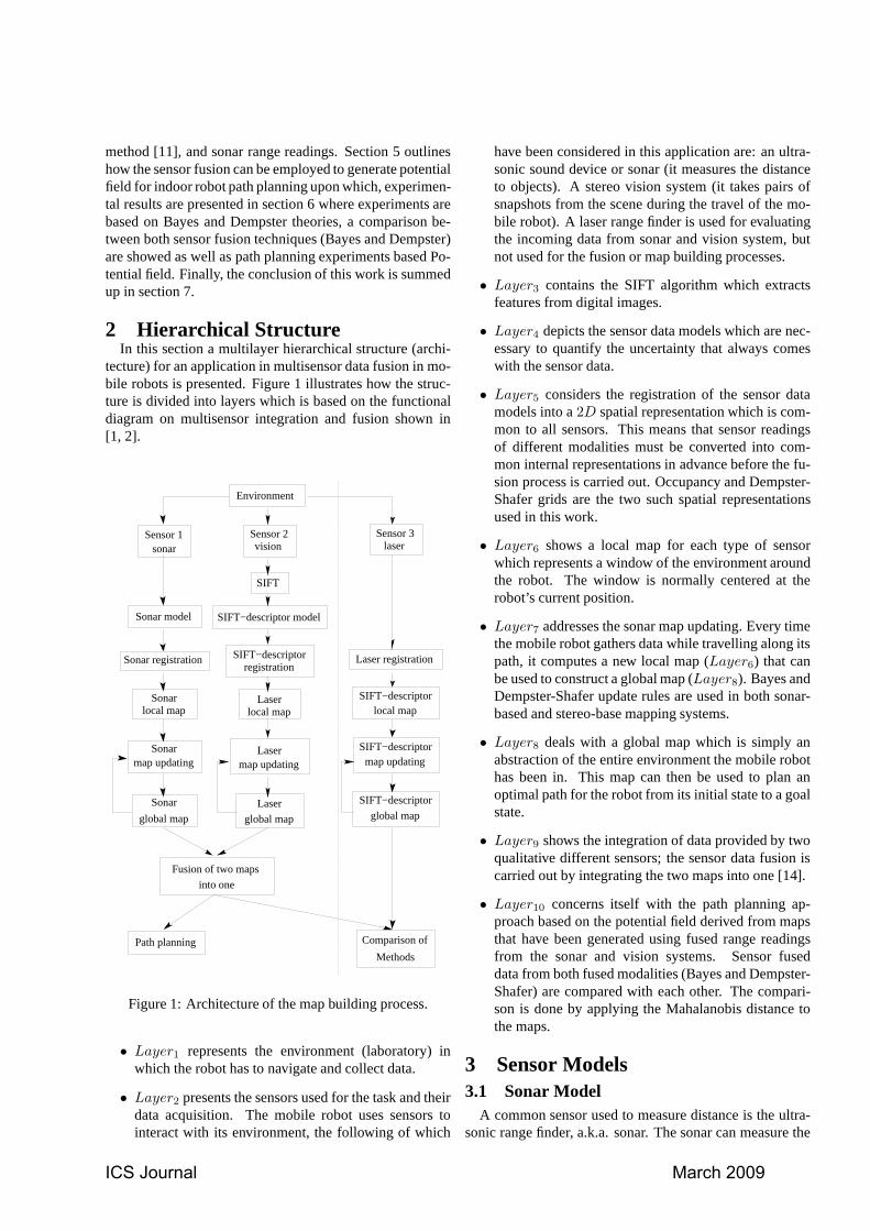
2 Hierarchical StructureIn this section a multilayer hierarchical structure (archi-

tecture) for an application in multisensor data fusion in mo-bile robots is presented. Figure 1 illustrates how the struc-ture is divided into layers which is based on the functionaldiagram on multisensor integration and fusion shown in[1, 2].

Environment

Fusion of two maps

into one

Sensor 3laser

Laser registration

SIFT−descriptorlocal map

SIFT−descriptormap updating

SIFT−descriptor

global map

Path planning Comparison of

Methods

Sensor 1sonar

Sonar model

Sonar registration

Sonarlocal map

Sonarmap updating

Sonar

global map

SIFT

Sensor 2vision

SIFT−descriptor model

SIFT−descriptorregistration

Laserlocal map

Lasermap updating

Laser

global map

Figure 1: Architecture of the map building process.

• Layer1 represents the environment (laboratory) inwhich the robot has to navigate and collect data.

• Layer2 presents the sensors used for the task and theirdata acquisition. The mobile robot uses sensors tointeract with its environment, the following of which

have been considered in this application are: an ultra-sonic sound device or sonar (it measures the distanceto objects). A stereo vision system (it takes pairs ofsnapshots from the scene during the travel of the mo-bile robot). A laser range finder is used for evaluatingthe incoming data from sonar and vision system, butnot used for the fusion or map building processes.

• Layer3 contains the SIFT algorithm which extractsfeatures from digital images.

• Layer4 depicts the sensor data models which are nec-essary to quantify the uncertainty that always comeswith the sensor data.

• Layer5 considers the registration of the sensor datamodels into a2D spatial representation which is com-mon to all sensors. This means that sensor readingsof different modalities must be converted into com-mon internal representations in advance before the fu-sion process is carried out. Occupancy and Dempster-Shafer grids are the two such spatial representationsused in this work.

• Layer6 shows a local map for each type of sensorwhich represents a window of the environment aroundthe robot. The window is normally centered at therobot’s current position.

• Layer7 addresses the sonar map updating. Every timethe mobile robot gathers data while travelling along itspath, it computes a new local map (Layer6) that canbe used to construct a global map (Layer8). Bayes andDempster-Shafer update rules are used in both sonar-based and stereo-base mapping systems.

• Layer8 deals with a global map which is simply anabstraction of the entire environment the mobile robothas been in. This map can then be used to plan anoptimal path for the robot from its initial state to a goalstate.

• Layer9 shows the integration of data provided by twoqualitative different sensors; the sensor data fusion iscarried out by integrating the two maps into one [14].

• Layer10 concerns itself with the path planning ap-proach based on the potential field derived from mapsthat have been generated using fused range readingsfrom the sonar and vision systems. Sensor fuseddata from both fused modalities (Bayes and Dempster-Shafer) are compared with each other. The compari-son is done by applying the Mahalanobis distance tothe maps.

3 Sensor Models3.1 Sonar Model

A common sensor used to measure distance is the ultra-sonic range finder, a.k.a. sonar. The sonar can measure the

ICS Journal March 2009

distance from the transducer to an object quite accurately.However, it can not estimate at what angle within the sonarcone the pulse was reflected. Hence, there will be someuncertainty about the angle at which the obstacle was mea-sured. A wide range of sonar models have been developedin the past years by various researchers, [3], [4], [12], and[15]. Taking the starting point in these methods, a gridG

of cells Ci,j , 1 ≤ i = x ≤ xmax, 1 ≤ j = y ≤ ymax isdefined in front of the sensor.

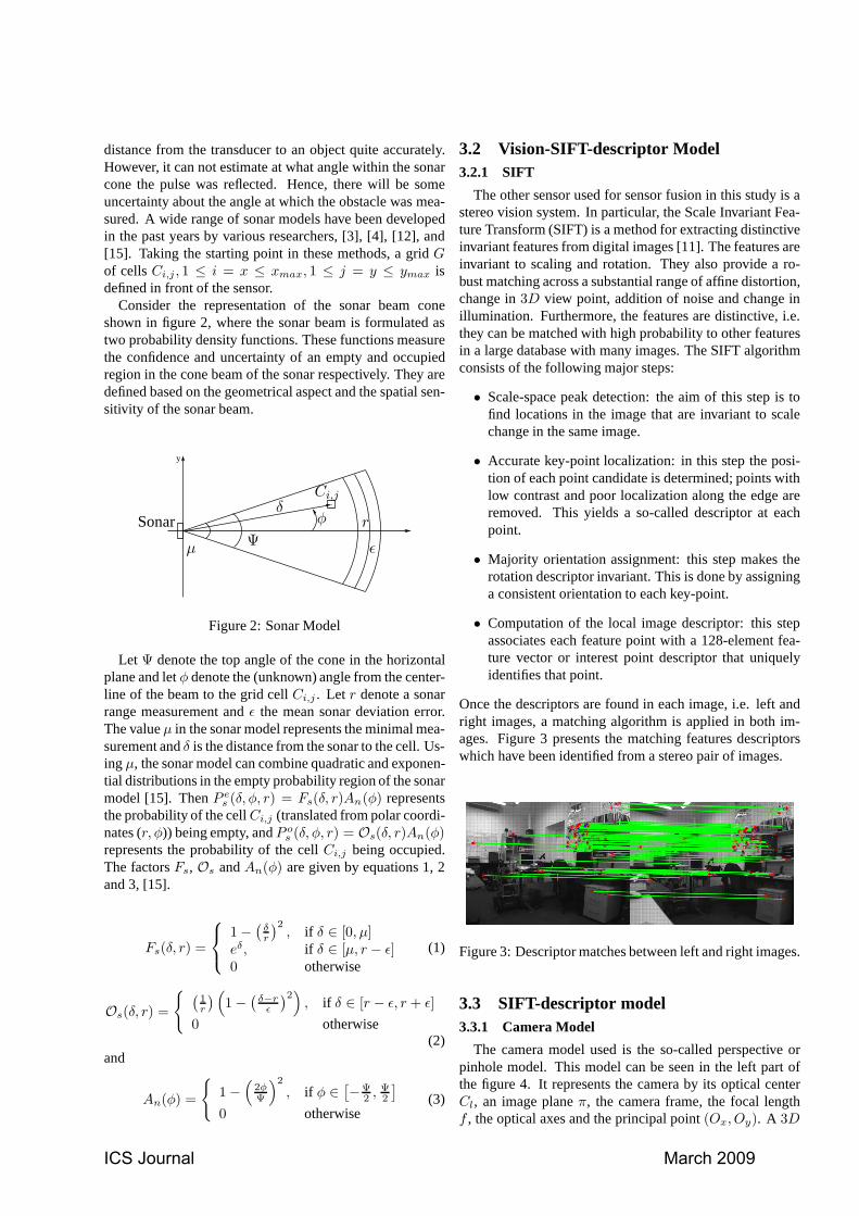
Consider the representation of the sonar beam coneshown in figure 2, where the sonar beam is formulated astwo probability density functions. These functions measurethe confidence and uncertainty of an empty and occupiedregion in the cone beam of the sonar respectively. They aredefined based on the geometrical aspect and the spatial sen-sitivity of the sonar beam.

y

ǫ

rSonar φ

µ

δ

Ψ

Ci,j

Figure 2: Sonar Model

Let Ψ denote the top angle of the cone in the horizontalplane and letφ denote the (unknown) angle from the center-line of the beam to the grid cellCi,j . Let r denote a sonarrange measurement andǫ the mean sonar deviation error.The valueµ in the sonar model represents the minimal mea-surement andδ is the distance from the sonar to the cell. Us-ing µ, the sonar model can combine quadratic and exponen-tial distributions in the empty probability region of the sonarmodel [15]. ThenP e

s (δ, φ, r) = Fs(δ, r)An(φ) representsthe probability of the cellCi,j (translated from polar coordi-nates (r, φ)) being empty, andP o

s (δ, φ, r) = Os(δ, r)An(φ)represents the probability of the cellCi,j being occupied.The factorsFs, Os andAn(φ) are given by equations 1, 2and 3, [15].

Fs(δ, r) =

1 −(

δr

)2, if δ ∈ [0, µ]

eδ, if δ ∈ [µ, r − ǫ]0 otherwise

(1)

Os(δ, r) =

{

(

1r

)

(

1 −(

δ−rǫ

)2)

, if δ ∈ [r − ǫ, r + ǫ]

0 otherwise(2)

and

An(φ) =

{

1 −(

2φΨ

)2

, if φ ∈[

−Ψ2 , Ψ

2

]

0 otherwise(3)

3.2 Vision-SIFT-descriptor Model3.2.1 SIFT

The other sensor used for sensor fusion in this study is astereo vision system. In particular, the Scale Invariant Fea-ture Transform (SIFT) is a method for extracting distinctiveinvariant features from digital images [11]. The features areinvariant to scaling and rotation. They also provide a ro-bust matching across a substantial range of affine distortion,change in3D view point, addition of noise and change inillumination. Furthermore, the features are distinctive,i.e.they can be matched with high probability to other featuresin a large database with many images. The SIFT algorithmconsists of the following major steps:

• Scale-space peak detection: the aim of this step is tofind locations in the image that are invariant to scalechange in the same image.

• Accurate key-point localization: in this step the posi-tion of each point candidate is determined; points withlow contrast and poor localization along the edge areremoved. This yields a so-called descriptor at eachpoint.

• Majority orientation assignment: this step makes therotation descriptor invariant. This is done by assigninga consistent orientation to each key-point.

• Computation of the local image descriptor: this stepassociates each feature point with a 128-element fea-ture vector or interest point descriptor that uniquelyidentifies that point.

Once the descriptors are found in each image, i.e. left andright images, a matching algorithm is applied in both im-ages. Figure 3 presents the matching features descriptorswhich have been identified from a stereo pair of images.

Figure 3: Descriptor matches between left and right images.

3.3 SIFT-descriptor model3.3.1 Camera Model

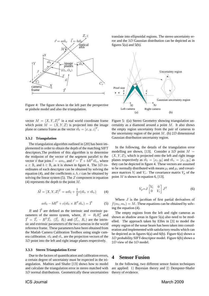
The camera model used is the so-called perspective orpinhole model. This model can be seen in the left part ofthe figure 4. It represents the camera by its optical centerCl, an image planeπ, the camera frame, the focal lengthf , the optical axes and the principal point(Ox, Oy). A 3D

ICS Journal March 2009

f

~l = b~ml

opticalaxis

M

y

Y imageplanes

(Ox, Oy)π

x

~nCl

X

~T

Cr

~ml

~r = a~mr

~mr

cameraframe

Z, z

Figure 4: The figure shows in the left part the perspectiveor pinhole model and also the triangulation.

vectorM = [X, Y, Z]T in a real world coordinate framewhich pointM = (X, Y, Z) is projected into the imageplane or camera frame as the vector~ml = [x, y, z]T .

3.3.2 Triangulation

The triangulation algorithm outlined in [20] has been im-plemented in order to obtain the depth of the matching SIFTdescriptors.The problem of this algorithm is to determinethe midpoint of the vector of the segment parallel to thevector~n that joins~l = aml, and~r = ~T + bRT ~mr, wherea ∈ R, andb ∈ R, as it is shown in figure 4. The3D co-ordinates of each descriptor can be obtained by solving theequation (4), and the coefficientsa, b, c can be obtained bysolving the linear system (5). TheZ component in equation(4) represents the depth to the pointM .

~M = [X, Y, Z]T = a~ml +1

2c(~mr × ~mr) (4)

a~ml − bRT + c(~ml × RT ~mr) = ~T (5)

R and ~T are defined as the intrinsic and extrinsic pa-rameters of the stereo system, where,R = RlR

Tr and

~T = ~Tr − RT ~Tl. (~Tl, Rl) and (~Tr, Rr) are the intrin-sic and extrinsic parameters of the two cameras in the worldreference frame. These parameters have been obtained fromthe Matlab Camera Calibration Toolbox using single cam-era calibration.~ml and~mr are the projection vectors of the3D point into the left and right image planes respectively.

3.3.3 Stereo Triangulation Error

Due to the factors of quantification and calibration errors,a certain degree of uncertainty must be expected in the tri-angulation. Mathies and Shafer [13] shows how to modeland calculate the triangulation error in stereo matched with3D normal distributions. Geometrically these uncertainties

translate into ellipsoidal regions. The stereo uncertainty er-ror and the3D Gaussian distribution can be depicted as infigures 5(a) and 5(b).

M

(a) (b)

Uncertainty region

Gaussian uncertainty region

zzPixel size

Xl XrLeft camera Right camera

Figure 5: ((a) Stereo Geometry showing triangulation un-certainty as a diamond around a pointM . It also showsthe empty region uncertainty from the pair of cameras tothe uncertainty region of the pointM . (b) 2D dimensionalGaussian distribution uncertainty region.

In the following, the details of the triangulation errormodelling are shown, [13]. Consider a3D point M =(X, Y, Z), which is projected onto the left and right imageplanes respectively as~ml = [xl, yl] and ~mr = [xr , yr] asthey can be depicted in figure 4. These vectors are assumedto be normally distributed with meansµl andµr and covari-ance matricesVl andVr. The covariance matrixVp of thepointM is shown in equation 6, [13].

Vp=J

[

Vl 00 Vr

]

JT (6)

Where J is the jacobian of first partial derivatives off(ml, mr) = M . These equations can be obtained by solv-ing the equation (4).

The empty regions from the left and right cameras asshown as shadow areas in figure 5(a) also need to be mod-elled. The approach taken by Elfes in [3] to model theempty region of the sonar beam has been taken into consid-eration and implemented with satisfactory results which canbe depicted as in figures 6(a) and 6(b). Figure 6(a) shows a3D probability SIFT-descriptor model. Figure 6(b) shows a2D view of the3D model.

4 Sensor FusionIn the following, two different sensor fusion techniques

are applied:1) Bayesian theory and2) Dempster-Shafertheory of evidence.

ICS Journal March 2009

(a) (b)

Figure 6: (a)3D view of the SIFT-descriptor probabil-ity model. (b)2D view of the SIFT-descriptor probabilitymodel.

4.1 Bayes Theory4.1.1 Bayes Update Formula

Elfes and Matthies [3] have proposed in their previ-ous work the use of a recursive Bayes formula to up-date the occupancy grid for multiple sensor observations(r1, ....., rt, rt+1). When this formula is transferred to theoccupancy grid framework, the following is obtained:

P o =P o

s P om

P os P o

m + (1 − P os )(1 − P o

m)(7)

• P om and1−P o

m are the prior probabilities that a cell isoccupied and empty respectively; they are taken fromthe existing map.

• P os is the conditional probability that a sensor would

return the sensor reading given the state of the cell be-ing occupied. This conditional probability is given bythe probabilistic sensor model(P o

s (δ, φ, r)).

• P o is the conditional probability that a cell is occupiedbased on the past sensor readings. It is the new esti-mate.

A new sensor reading, introduces additional informationabout the state of the cellCi,j . This information is doneby the sensor modelP o

s and it is combined with the mostrecent probability estimate stored in the cell. This combi-nation is done by the recursive Bayes’ rule based on thecurrent set of readingsrt = (rt, rt−n, ...., r0) to give a newestimateP o. It is worth noting that when initializing themap an equal probability to each cellCi,j must be assigned.In other words, the initial map cell prior probabilities areP o

m = 1 − P om = 0.5 ∀Ci,j .

4.1.2 Fusion of Sensors With Two Occupancy Grids

In this method, an occupancy grid based on the Bayes’rule is constructed for each sensor type, which will then befused to build up the resulting grid map. Afterwards, thecells in each grid map are modified in order to reinforce thecell probability of being occupied, [14]:

• The probability of a cellCi,j being occupied is set toone if it is higher than a predefined thresholdTo.

• The probability of a cellCi,j being occupied is rein-force if it is between the interval[ 12 , To]. The rein-forcement strength the probability of a cell being oc-cupied.

• Otherwise the value in the cellCi,j remains.

More precisely, the resulting grid map is computed in twosteps.

Firstly, probability values in the grid maps are modifiedfor each sensor type using the following expression:

P on=1,2(c) =

1 for P o(c) > To,P o(c)+To−1

2·To−1 for P o(c) ∈ [ 12 , To]

P o(c) otherwise(8)

WhereP o(c) is the probability of the cellCi,j being occu-pied. P o

1 (c) is the modified probability of occupancy fromthe first sensor andP o

2 (c) is the modified probability of oc-cupancy from the second sensor.

Secondly, the computed values are then inserted inBayes’ rule to obtain the occupied fused probabilityP o

f (c)of the cellCi,j in the resulting grid.

P of (c) =

P o1 (c)P o

2 (c)

P o1 (c)P o

2 (c) + (1 − P o1 (c)(1 − P o

2 (c))(9)

4.2 Dempster-Shafer TheoryThe second method concerns Dempster-Shafer theory of

evidence. This theory was proposed by Glenn Shafer [5] asan extension of the work presented in [6] and [7].

Dempster-Shafer theory is mainly characterized by aframe of discernment(FOD = Θ), a basic probabilityassignment function(bpa), a belief function(Bel) and aplausibility(PLS) function. These are tied together via theso-called Dempster’s rule of combination [8].

Each proposition inΘ is called a singleton.2Θ is calledthe power set ofΘ. Any subset ofΘ is called a hypoth-esis. Applying the notion of frames of discernment to anoccupancy grid yields a set of framesΘi,j = {o, e}; wherei, j represents an individual cell in the grid. LetA de-note the subsets of the power set of2Θi,j = 2{o,e} ={

{∅}, {o}, {e}, {o, e}}

; where {∅} and {o, e} are theempty and thedisjunction or dontknow subsets, respec-tively. {o} and{e} denote the probabilities of the cell beingoccupied or empty, respectively. Thequantum of beliefisdistributed asBel(A) = m(∅)+m(o)+m(e)+m(o, e) =1, [5]. Finally, the functionm : 2Θ → [0, 1] is called thebasic probability assignment. and must satisfy the follow-ing criteria.

∑

A⊂2Θ

m(A) = 1 (10)

m(∅) = 0 (11)

Equation (11) reflects the fact that no belief is assigned to∅.In order to obtain the total evidence assigned toA, one must

ICS Journal March 2009

add tom(A) the quantitiesm(B) for all proper subsetsBof A.

Bel(A) =∑

∀B:B⊆A

m(B) (12)

In [5], the notion ofplausibility or upper probability ofA is defined as1−Bel(¬A); where(¬A) is used to denotethe set theoretic complement ofA. Bel(¬A) is the disbe-lief of the hypothesis ofA. Consequently,Pls(A) can bethought of as the amount of evidence that does not supportits negation. All in all, this sums up to

Pls(A) = 1 − Bel(¬A) = 1 −∑

∀B:B 6⊂A

m(B) (13)

Notice thatBel(A) ≤ Pls(A) for any givenA.The above assumptions brings up with a formulation of a

formal Dempster’s rule of combination.SupposeBel1 and Bel2 are belief functions over the

same frame of discernmentΘ, with basic probability as-signment in each focal element, e.g.{m(A1), · · ·, m(Ak)}and{m(B1), · · ·, m(Bl)} respectively. The belief functiongiven bym(Ck) is called orthogonal sum ofBel1 andBel2and is represented asBel1 ⊕ Bel2,

m(Ck) =

∑

∀Ai,Bj∈2Θi,j :Ai∩Bi=Ck;Ck 6=∅ m(Ai)m(Bj)

1 −∑

∀Ai,Bj∈2Θi,j :Ai∩Bj=∅ m(Ai)m(Bj)

(14)Some remarks are drawn. These two belief functions areindependent and have at least one focal element in common.The two belief functions can be combined by finding thefocal intersections for eachCk, whereC is the set of allsubsets produced byAi ∩Bj . The denominator in equation14 is the normalisation term.

When using Dempster’s rule of combination to update agrid map for each cellCi,j lying in the main lobe of thesonar model and for each interpreted sensor reading, equa-tion (14) becomes:

mo =mG

o mSo + mG

o mSo,e + mG

o,emSo

1 − mGe mS

o − mGo mS

e

(15)

me =mG

e mSe + mG

e mSo,e + mG

o,emSe

1 − mGe mS

o − mGo mS

e

(16)

mo,e =mG

o,emSo,e

1 − mGe mS

o − mGo mS

e

(17)

The quantitiesmSo , mS

e andmSo,e are obtained from sen-

sor models, whilemGo , mG

e andmGo,e are obtained from the

existing grid map. Note thatmGo,e = 1 − mG

o − mGe , and

mSo,e = 1 − mS

o − mSe . mo, mo, andmo,e are the new

updates. All cellsCi,j in the Shafer grid map are initial-ized as stated in (18) since there is noapriori knowledge ofevidence.

mGo = 0

mGe = 0

mGo,e = 1

∀Ci,j ∈ G (18)

The above assumption means total ignorance about thestate of each cell. However, when the mobile robot is mov-ing and gathering data from the environment it uses this datato update the map using Dempster’s rule of combinationequations 15, 16, and 17.

The lack of ignorance is depicted in the expression (19),and simply expresses an exact knowledge of the environ-ment.

mGo + mG

e = 1

mGo,e = 0

}

∀Ci,j ∈ G (19)

5 Path Planning Using PotentialField

The main idea of potential field is to discretize the con-figuration spaceW of the robotA into a regular grid andsearch for an appropriate pathτ within that grid. In thisapproach, the robot is considered as a particle in the con-figuration space moving under the influence of an artificialpotential fieldU . The potential field consists of the sum ofan attractive potential field generated by the goal and a re-pulsive potential generated by the obstacles [18], as seen inequation (20).

U(~q) = Uatt(~q) + Urep(~q) (20)

where~q = [x, y, θ]T (a compact set closed and bounded inW) which is the current state of the robot (a.k.a.configura-tion). An example of an attractive and a repulsive potentialfield functions can be depicted in equations 21 and 22.

Uatt(~q) =1

2ξρ2

goal(~q) (21)

Urep(~q) =

12η

(

1ρ(~q) −

1ρ0

)2

if ρ(~q) ≤ ρ0,

0 if ρ(~q) > ρ0,

(22)

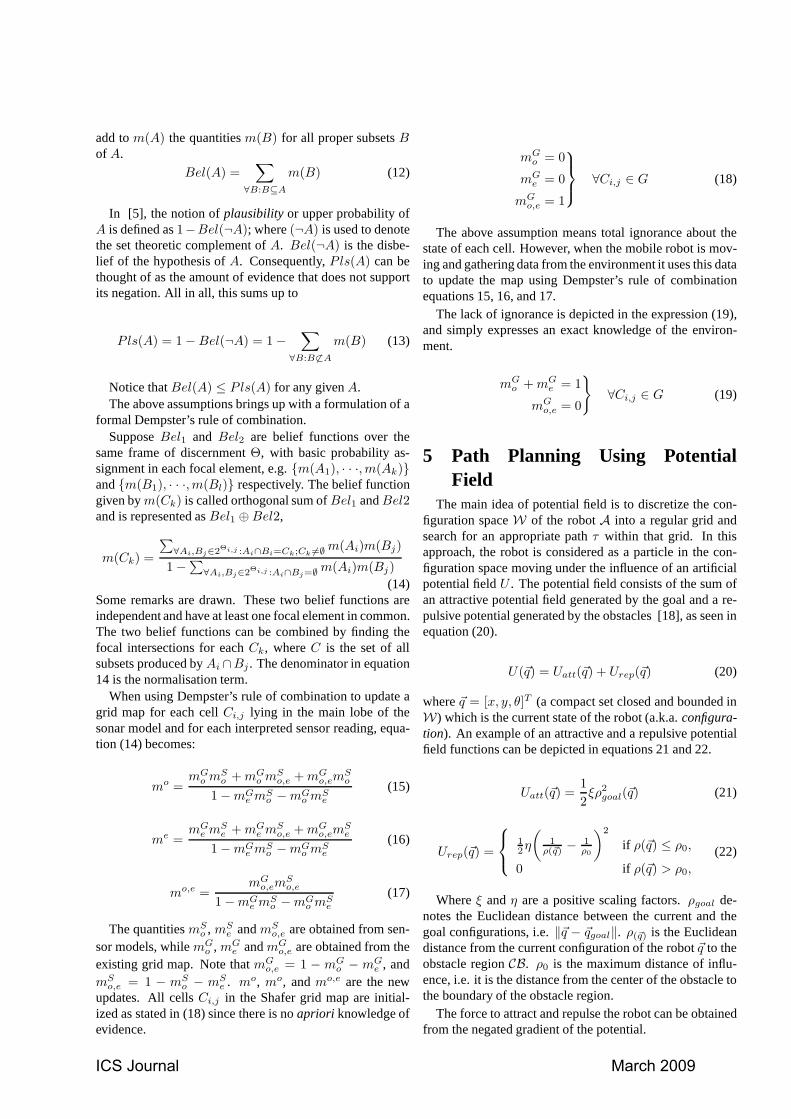
Whereξ andη are a positive scaling factors.ρgoal de-notes the Euclidean distance between the current and thegoal configurations, i.e.‖~q − ~qgoal‖. ρ(~q) is the Euclideandistance from the current configuration of the robot~q to theobstacle regionCB. ρ0 is the maximum distance of influ-ence, i.e. it is the distance from the center of the obstacle tothe boundary of the obstacle region.

The force to attract and repulse the robot can be obtainedfrom the negated gradient of the potential.

ICS Journal March 2009

~F = −∇U(~q) = −

[

∂U(~q)∂x

∂U(~q)∂y

]

= −

[

∂Uatt(~q)∂x

+∂Urep(~q)

∂x∂Uatt(~q)

∂y+

∂Urep(~q)∂y

]

= −

[

∂Uatt(~q)∂x

∂Uatt(~q)∂y

]

−

[

∂Urep(~q)∂x

∂Urep(~q)∂y

]

= ~Fatt(~q) + ~Frep(~q) (23)

The potential field can be obtained mathematically whenthe position of the obstacles are precisely identified. Theobstacles generate a repulsive potential field which makesthe robot navigate far from the obstacles. The other op-tion considered in this article consists of moving the robotthrough the obstacles generated by, applying the sensor fu-sion techniques (Bayes and Dempster’s rules) to the sensorreadings. The attractive potential field is added to the po-tential field generated from the environment using sensorreadings.

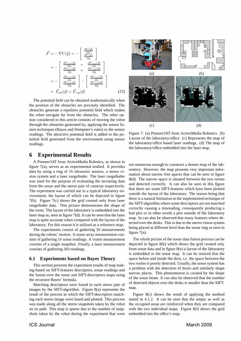
6 Experimental ResultsA Pioneer3AT from ActiveMedia Robotics, as shown in

figure 7(a), serves as an experimental testbed. It providesdata by using a ring of16 ultrasonic sensors, a stereo vi-sion system and a laser rangefinder. The laser rangefinderwas used for the purpose of evaluating the incoming datafrom the sonar and the stereo pair of cameras respectively.The experiment was carried out in a typical laboratory en-vironment, the layout of which can be depicted in figure7(b). Figure 7(c) shows the grid created only from laserrangefinder data. This picture demonstrates the shape ofthe room. The layout of the laboratory is embedded into thelaser map as, seen in figure 7(d). It can be seen that the lasermap is quite accurate when compared with the layout of thelaboratory. For this reason it is utilized as a reference map.

The experiments consist of gathering30 measurementsduring the robots’ motion. A sonar array measurement con-sists of gathering16 sonar readings. A vision measurementconsists of a single snapshot. Finally, a laser measurementconsists of gathering360 readings.

6.1 Experiments based on Bayes TheoryThis section presents the experiment results of map mak-

ing based on SIFT-features descriptors, sonar readings andthe fusion over the sonar and SIFT-descriptors maps usingthe recursive Bayes’ formula.

Matching descriptors were found in each stereo pair ofimages by the SIFT-algorithm. Figure 8(a) represents theresult of the process in which the SIFT-descriptors match-ing each stereo image were fused and plotted. This processwas made along all the stereo snapshots taken by the roboton its path. This map is sparse due to the number of snap-shots taken by the robot during the experiment that were

(a) (b)

(c) (d)

Figure 7: (a) Pioneer3AT from ActiveMedia Robotics. (b)Layout of the laboratory/office. (c) Represents the map ofthe laboratory/office based laser readings. (d) The map ofthe laboratory/office embedded into the laser map.

not numerous enough to construct a denser map of the lab-oratory. However, the map presents very important infor-mation about narrow free spaces that can be seen in figure8(d). The narrow space is situated between the two roomsand detected correctly. It can also be seen in this figurethat there are some SIFT-features which have been plottedoutside the layout of the laboratory. The reason being thatthere is a natural limitation in the implemented technique ofthe SIFT-algorithm where some descriptors are not matchedcorrectly causing a misreading, consequently producing abad plot or in other words a plot outside of the laboratorymap. In can also be observed that many features where de-tected over the desks. This is due to the stereo vision systembeing placed at different level than the sonar ring as seen infigure 7(a).

The whole picture of the sonar data fusion process can bedepicted in figure 8(b) which shows the grid created onlyfrom sonar data and in figure 8(e) a layout of the laboratoryis embedded in the sonar map. It can be noticed that thespace before and inside the door, i.e. the space between thetwo rooms is poorly detected. Usually, the sonar system hasa problem with the detection of doors and similarly shapenarrow places. This phenomenon is created by the shapeof the sonar beam. It can also be observed that the numberof detected objects over the desks is smaller than the SIFT-map.

Figure 8(c) shows the result of applying the methodstated in 4.1.2. It can be seen that the empty as well asthe occupied areas are reinforced when they are comparedwith the two individual maps. Figure 8(f) shows the gridembedded into the office’s map.

ICS Journal March 2009

(a) (b) (c)

(d) (e) (f)

Figure 8: Maps generated from applying Bayes theory tointerpreted sensor readings. Top row: (a) SIFT-descriptormap. (b) sonar map. (c) SIFT-sonar fused maps ; Bottomrow: maps with office layout superimposed.

6.2 Experiments based on Dempster-ShaferTheory

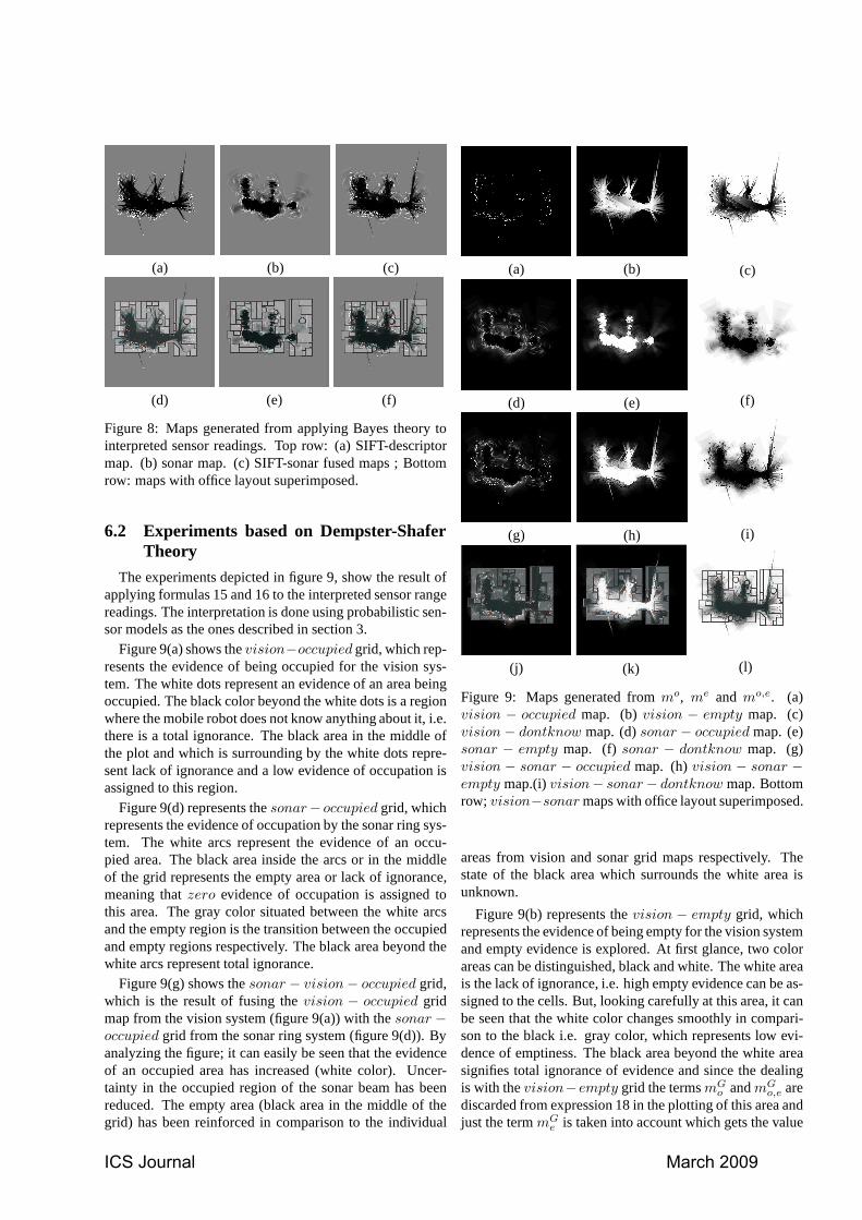
The experiments depicted in figure 9, show the result ofapplying formulas 15 and 16 to the interpreted sensor rangereadings. The interpretation is done using probabilistic sen-sor models as the ones described in section 3.

Figure 9(a) shows thevision−occupied grid, which rep-resents the evidence of being occupied for the vision sys-tem. The white dots represent an evidence of an area beingoccupied. The black color beyond the white dots is a regionwhere the mobile robot does not know anything about it, i.e.there is a total ignorance. The black area in the middle ofthe plot and which is surrounding by the white dots repre-sent lack of ignorance and a low evidence of occupation isassigned to this region.

Figure 9(d) represents thesonar− occupied grid, whichrepresents the evidence of occupation by the sonar ring sys-tem. The white arcs represent the evidence of an occu-pied area. The black area inside the arcs or in the middleof the grid represents the empty area or lack of ignorance,meaning thatzero evidence of occupation is assigned tothis area. The gray color situated between the white arcsand the empty region is the transition between the occupiedand empty regions respectively. The black area beyond thewhite arcs represent total ignorance.

Figure 9(g) shows thesonar − vision − occupied grid,which is the result of fusing thevision − occupied gridmap from the vision system (figure 9(a)) with thesonar −occupied grid from the sonar ring system (figure 9(d)). Byanalyzing the figure; it can easily be seen that the evidenceof an occupied area has increased (white color). Uncer-tainty in the occupied region of the sonar beam has beenreduced. The empty area (black area in the middle of thegrid) has been reinforced in comparison to the individual

(a) (b) (c)

(d) (e) (f)

(g) (h) (i)

(j) (k) (l)

Figure 9: Maps generated frommo, me and mo,e. (a)vision − occupied map. (b)vision − empty map. (c)vision − dontknow map. (d)sonar − occupied map. (e)sonar − empty map. (f) sonar − dontknow map. (g)vision − sonar − occupied map. (h)vision − sonar −empty map.(i)vision− sonar − dontknow map. Bottomrow; vision−sonar maps with office layout superimposed.

areas from vision and sonar grid maps respectively. Thestate of the black area which surrounds the white area isunknown.

Figure 9(b) represents thevision − empty grid, whichrepresents the evidence of being empty for the vision systemand empty evidence is explored. At first glance, two colorareas can be distinguished, black and white. The white areais the lack of ignorance, i.e. high empty evidence can be as-signed to the cells. But, looking carefully at this area, it canbe seen that the white color changes smoothly in compari-son to the black i.e. gray color, which represents low evi-dence of emptiness. The black area beyond the white areasignifies total ignorance of evidence and since the dealingis with thevision−empty grid the termsmG

o andmGo,e are

discarded from expression 18 in the plotting of this area andjust the termmG

e is taken into account which gets the value

ICS Journal March 2009

of 0.Figure 9(e) shows thesonar− empty grid, which repre-

sents the evidence of being empty for the sonar ring system.The white area represents the empty region. The gray areais the transition between the empty and occupied regions.The black area beyond the white area signifies a total igno-rance of evidence.

Figure 9(h) shows the result of fusing the resultingvision − empty grid map from the vision system (figure9(b) with the resultingsonar − empty grid map from thesonar ring system (figure 9(e)). Looking carefully at the fig-ure; it can easily be noticed that the evidence of an emptyarea (white color in the middle of the plot) has increased, i.ethe empty area has been reinforced. It can be seen when itis compared with the individual areas fromvision−empty

andsonar− empty grid maps respectively. The black areasurrounding the white area is the total ignorance. Thereis a gray area between the black and white areas which isthe transition of emptiness (white) to the total of ignorance(black). There are some black zones within the gray area,which represent strong evidence of occupation.

Figure 9(c) shows thevision − dontknow grid which,represents the evidence of disjunction for the vision sys-tem. The black area in the middle of the map signifies lackof ignorance. Although, one can see that the black colorchanges smoothly from black (middle of the map) to grayand then to black (dot pots) and then to white. Representingignorance of evidence.

Figure 9(f) shows the result of applying equation 17 tothe interpreted sonar data which generates thesonar −dontknow grid. The meaning of the colors are explained inthe following. The black color means lack of ignorance andhigh evidence can be assigned to the empty area. The graycolor is the level of transition from lack of ignorance to to-tal ignorance, meaning that the empty evidence goes frombeing high to low. The dark arcs inside the cones of thesonar beam represent strong evidence of occupation. Thewhite area beyond the cones of the sonar beam representstotal ignorance of evidence.

Figure 9(i) shows thesonar − vision − dontknow

grid, which is the result of fusing the resultingvision −dontknow grid map from the vision system (figure9(c))with the resultingsonar − dontknow grid map from thesonar ring system (figure 9(f)). The black area in the middleof the plot signifies lack of ignorance. Thus a high degreeof empty evidence can be assigned to that area. The grayarea is the transition from the empty area to the occupiedarea or in other words, it is the transition from lack of ig-norance to total ignorance. During the transition, gray arcsand black dots can be seen. The arcs are the occupied re-gion of the sonar beam; the more black the arcs are the morethe evidence of the arcs being occupied. The black dots arethe SIFT-features, which reinforce the occupied region ofthe sonar beam. The white surface means total ignorance ofevidence.

Figures 9(j), 9(k) and 9(l) show thevision − sonar −occupied, vision− sonar− empty andvision− sonar−

dontknow grid maps embedded into laboratory map re-spectively.

6.3 Mahalanobis Distance ComparisonThe Mahalanobis distance measure approach was intro-

duced by [25] in 1936. It is based on correlations betweenrandom vectors. It differs from Euclidean distance in that ittakes into account the correlations of the data set.

Lets ~x and~y be two random vectors, the MahalanobisdistancedM from a vector~y to the vector~x is the distancefrom ~y to ~x, the centroid of~x, weighted according toCx,the covariance matrix of~x, so that,

dM =((~y − ~x)′Cx

−1(~y − ~x))1

2 (24)

Where :

~x =1

2

nx∑

i=1

~xi (25)

Cx =1

nx − 1

nx∑

1

(~xi − ~x)(~xi − ~x)′ (26)

The Mahalanobis distance from a SIFT, sonar, and, SIFT-sonar vectors to a laser, is computed in the following. Theelements of the SIFT, sonar, and SIFT-sonar vectors are thecoordinates of the occupied cells of their respective maps.The elements of the laser vector are also the coordinates ofthe occupied cells of its respective map. The laser is takenas a true parameter vector to be compared with the othervectors.

The Mahalanobis distance is computed in squared unitsof each observation in the reference sample~x. A unit has avalue of5 cm which is the size of a single cell in the grid.

A 2D grid plot (laser& SIFT), which has been generatedby the laser grid map and the SIFT grid map based on Bayesapproach, is presented in figure 10(a). The red squares cor-respond to the occupied laser cells. The asterisks representthe occupied cells by theSITF -descriptor grid map. Eachcolour represents a Mahalanobis distance to the laser vec-tor. The corresponding colour values of the distances arerepresented as a colour bar placed next to the map. Figure10(c) depicts the plot of the Mahalabobis distance from fig-ure 10(a). The same situation for the Dempster approach isdepicted in figures 10(b) and 10(d). A comparison of thesetwo plots reveals that both SIFT-descriptor grids based onBayes and Dempster approaches approximate the laser plot.The difference stems from the fact that the SIFT-feature al-gorithm finds features in the scene that the laser is not ableto find and vice versa, the laser& SIFT (Dempster) dis-tance plot is significantly less abundant than the laser&SIFT (Bayes) distance plot.

The situation where the sonar coordinates vector is takeninto account to compute the Mahalanobis distance to a lasercoordinates vector can be depicted in figure 11. The colourof the asterisks in figures 11(a) and 11(b) are yellow, blue,

ICS Journal March 2009

(a)

(c)

(b)

(d)

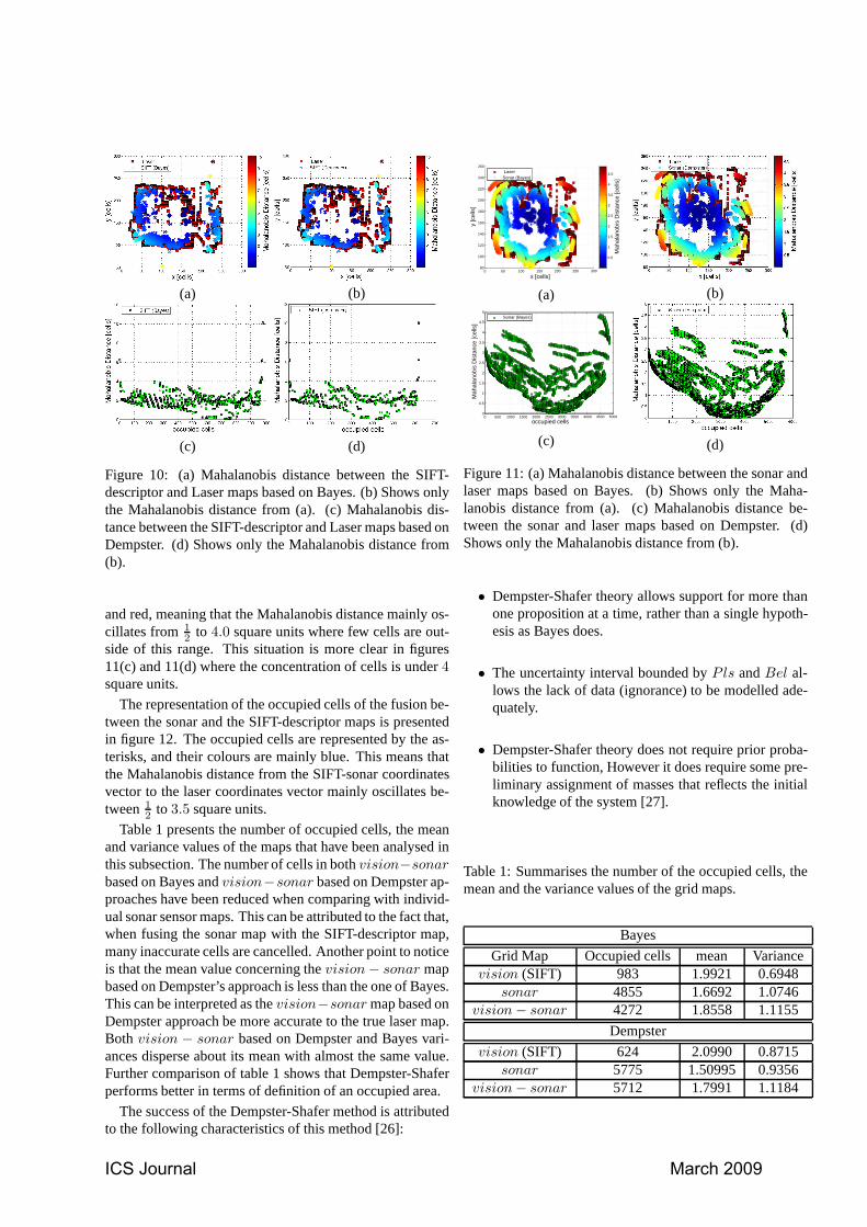
Figure 10: (a) Mahalanobis distance between the SIFT-descriptor and Laser maps based on Bayes. (b) Shows onlythe Mahalanobis distance from (a). (c) Mahalanobis dis-tance between the SIFT-descriptor and Laser maps based onDempster. (d) Shows only the Mahalanobis distance from(b).

and red, meaning that the Mahalanobis distance mainly os-cillates from1

2 to 4.0 square units where few cells are out-side of this range. This situation is more clear in figures11(c) and 11(d) where the concentration of cells is under4square units.

The representation of the occupied cells of the fusion be-tween the sonar and the SIFT-descriptor maps is presentedin figure 12. The occupied cells are represented by the as-terisks, and their colours are mainly blue. This means thatthe Mahalanobis distance from the SIFT-sonar coordinatesvector to the laser coordinates vector mainly oscillates be-tween1

2 to 3.5 square units.

Table 1 presents the number of occupied cells, the meanand variance values of the maps that have been analysed inthis subsection. The number of cells in bothvision−sonar

based on Bayes andvision−sonar based on Dempster ap-proaches have been reduced when comparing with individ-ual sonar sensor maps. This can be attributed to the fact that,when fusing the sonar map with the SIFT-descriptor map,many inaccurate cells are cancelled. Another point to noticeis that the mean value concerning thevision − sonar mapbased on Dempster’s approach is less than the one of Bayes.This can be interpreted as thevision−sonar map based onDempster approach be more accurate to the true laser map.Both vision − sonar based on Dempster and Bayes vari-ances disperse about its mean with almost the same value.Further comparison of table 1 shows that Dempster-Shaferperforms better in terms of definition of an occupied area.

The success of the Dempster-Shafer method is attributedto the following characteristics of this method [26]:

0 50 100 150 200 250 30080

100

120

140

160

180

200

220

240

260

x [cells]

y [c

ells

]

Mah

alan

obis

Dis

tanc

e [c

ells

]

0.5

1

1.5

2

2.5

3

3.5

4

4.5 Laser Sonar (Bayes)

(a)

0 500 1000 1500 2000 2500 3000 3500 4000 4500 50000

0.5

1

1.5

2

2.5

3

3.5

4

4.5

5

occupied cells

Mah

alan

obis

Dis

tanc

e [c

ells

]

Sonar (Bayes)

(c)

(b)

(d)

Figure 11: (a) Mahalanobis distance between the sonar andlaser maps based on Bayes. (b) Shows only the Maha-lanobis distance from (a). (c) Mahalanobis distance be-tween the sonar and laser maps based on Dempster. (d)Shows only the Mahalanobis distance from (b).

• Dempster-Shafer theory allows support for more thanone proposition at a time, rather than a single hypoth-esis as Bayes does.

• The uncertainty interval bounded byPls andBel al-lows the lack of data (ignorance) to be modelled ade-quately.

• Dempster-Shafer theory does not require prior proba-bilities to function, However it does require some pre-liminary assignment of masses that reflects the initialknowledge of the system [27].

Table 1: Summarises the number of the occupied cells, themean and the variance values of the grid maps.

Bayes

Grid Map Occupied cells mean Variancevision (SIFT) 983 1.9921 0.6948

sonar 4855 1.6692 1.0746vision − sonar 4272 1.8558 1.1155

Dempster

vision (SIFT) 624 2.0990 0.8715sonar 5775 1.50995 0.9356

vision − sonar 5712 1.7991 1.1184

ICS Journal March 2009

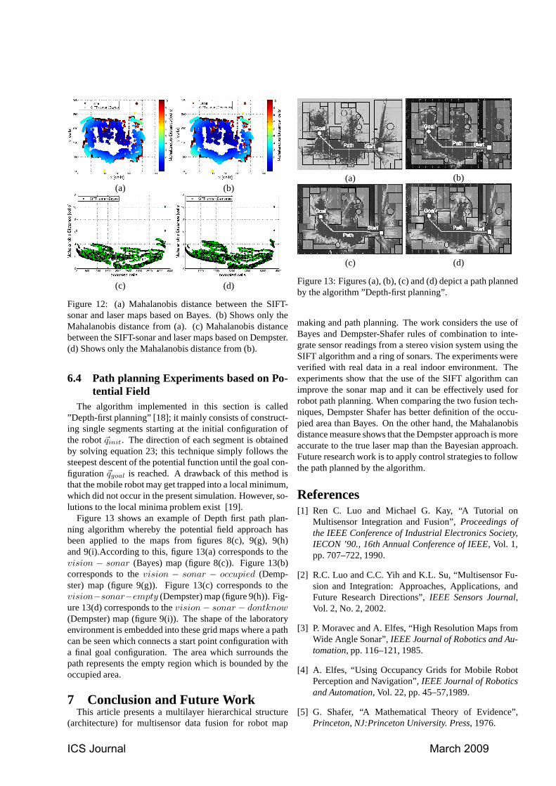
(a)

(c)

(b)

(d)

Figure 12: (a) Mahalanobis distance between the SIFT-sonar and laser maps based on Bayes. (b) Shows only theMahalanobis distance from (a). (c) Mahalanobis distancebetween the SIFT-sonar and laser maps based on Dempster.(d) Shows only the Mahalanobis distance from (b).

6.4 Path planning Experiments based on Po-tential Field

The algorithm implemented in this section is called”Depth-first planning” [18]; it mainly consists of construct-ing single segments starting at the initial configuration ofthe robot~qinit. The direction of each segment is obtainedby solving equation 23; this technique simply follows thesteepest descent of the potential function until the goal con-figuration~qgoal is reached. A drawback of this method isthat the mobile robot may get trapped into a local minimum,which did not occur in the present simulation. However, so-lutions to the local minima problem exist [19].

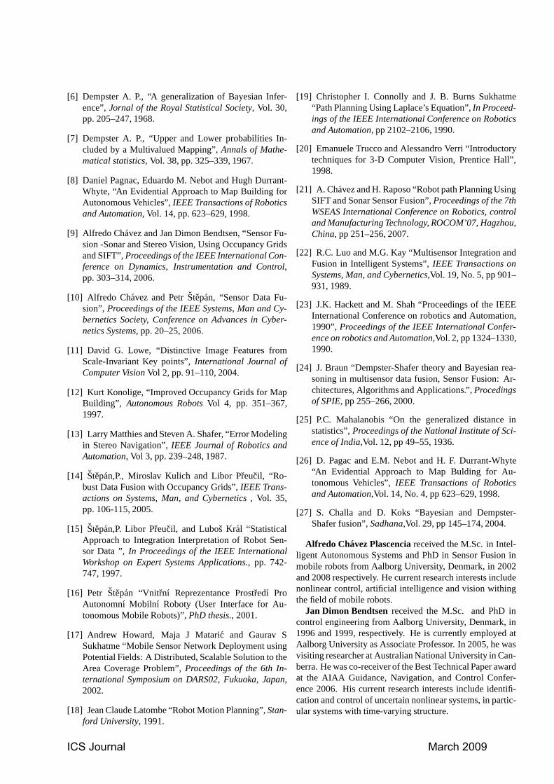
Figure 13 shows an example of Depth first path plan-ning algorithm whereby the potential field approach hasbeen applied to the maps from figures 8(c), 9(g), 9(h)and 9(i).According to this, figure 13(a) corresponds to thevision − sonar (Bayes) map (figure 8(c)). Figure 13(b)corresponds to thevision − sonar − occupied (Demp-ster) map (figure 9(g)). Figure 13(c) corresponds to thevision−sonar−empty (Dempster) map (figure 9(h)). Fig-ure 13(d) corresponds to thevision − sonar − dontknow

(Dempster) map (figure 9(i)). The shape of the laboratoryenvironment is embedded into these grid maps where a pathcan be seen which connects a start point configuration witha final goal configuration. The area which surrounds thepath represents the empty region which is bounded by theoccupied area.

7 Conclusion and Future WorkThis article presents a multilayer hierarchical structure

(architecture) for multisensor data fusion for robot map

(a)

(c)

(b)

(d)

Figure 13: Figures (a), (b), (c) and (d) depict a path plannedby the algorithm ”Depth-first planning”.

making and path planning. The work considers the use ofBayes and Dempster-Shafer rules of combination to inte-grate sensor readings from a stereo vision system using theSIFT algorithm and a ring of sonars. The experiments wereverified with real data in a real indoor environment. Theexperiments show that the use of the SIFT algorithm canimprove the sonar map and it can be effectively used forrobot path planning. When comparing the two fusion tech-niques, Dempster Shafer has better definition of the occu-pied area than Bayes. On the other hand, the Mahalanobisdistance measure shows that the Dempster approach is moreaccurate to the true laser map than the Bayesian approach.Future research work is to apply control strategies to followthe path planned by the algorithm.

References[1] Ren C. Luo and Michael G. Kay, “A Tutorial on

Multisensor Integration and Fusion”,Proceedings ofthe IEEE Conference of Industrial Electronics Society,IECON ’90., 16th Annual Conference of IEEE, Vol. 1,pp. 707–722, 1990.

[2] R.C. Luo and C.C. Yih and K.L. Su, “Multisensor Fu-sion and Integration: Approaches, Applications, andFuture Research Directions”,IEEE Sensors Journal,Vol. 2, No. 2, 2002.

[3] P. Moravec and A. Elfes, “High Resolution Maps fromWide Angle Sonar”,IEEE Journal of Robotics and Au-tomation, pp. 116–121, 1985.

[4] A. Elfes, “Using Occupancy Grids for Mobile RobotPerception and Navigation”,IEEE Journal of Roboticsand Automation, Vol. 22, pp. 45–57,1989.

[5] G. Shafer, “A Mathematical Theory of Evidence”,Princeton, NJ:Princeton University. Press, 1976.

ICS Journal March 2009

[6] Dempster A. P., “A generalization of Bayesian Infer-ence”,Jornal of the Royal Statistical Society, Vol. 30,pp. 205–247, 1968.

[7] Dempster A. P., “Upper and Lower probabilities In-cluded by a Multivalued Mapping”,Annals of Mathe-matical statistics, Vol. 38, pp. 325–339, 1967.

[8] Daniel Pagnac, Eduardo M. Nebot and Hugh Durrant-Whyte, “An Evidential Approach to Map Building forAutonomous Vehicles”,IEEE Transactions of Roboticsand Automation, Vol. 14, pp. 623–629, 1998.

[9] Alfredo Chavez and Jan Dimon Bendtsen, “Sensor Fu-sion -Sonar and Stereo Vision, Using Occupancy Gridsand SIFT”,Proceedings of the IEEE International Con-ference on Dynamics, Instrumentation and Control,pp. 303–314, 2006.

[10] Alfredo Chavez and PetrStepan, “Sensor Data Fu-sion”, Proceedings of the IEEE Systems, Man and Cy-bernetics Society, Conference on Advances in Cyber-netics Systems, pp. 20–25, 2006.

[11] David G. Lowe, “Distinctive Image Features fromScale-Invariant Key points”,International Journal ofComputer VisionVol 2, pp. 91–110, 2004.

[12] Kurt Konolige, “Improved Occupancy Grids for MapBuilding”, Autonomous RobotsVol 4, pp. 351–367,1997.

[13] Larry Matthies and Steven A. Shafer, “Error Modelingin Stereo Navigation”,IEEE Journal of Robotics andAutomation, Vol 3, pp. 239–248, 1987.

[14] Stepan,P., Miroslav Kulich and Libor Preucil, “Ro-bust Data Fusion with Occupancy Grids”,IEEE Trans-actions on Systems, Man, and Cybernetics, Vol. 35,pp. 106-115, 2005.

[15] Stepan,P. Libor Preucil, and Lubos Kral “StatisticalApproach to Integration Interpretation of Robot Sen-sor Data ”, In Proceedings of the IEEE InternationalWorkshop on Expert Systems Applications., pp. 742-747, 1997.

[16] Petr Stepan “Vnitrnı Reprezentance Prostredı ProAutonomnı Mobilnı Roboty (User Interface for Au-tonomous Mobile Robots)”,PhD thesis., 2001.

[17] Andrew Howard, Maja J Mataric and Gaurav SSukhatme “Mobile Sensor Network Deployment usingPotential Fields: A Distributed, Scalable Solution to theArea Coverage Problem”,Proceedings of the 6th In-ternational Symposium on DARS02, Fukuoka, Japan,2002.

[18] Jean Claude Latombe “Robot Motion Planning”,Stan-ford University, 1991.

[19] Christopher I. Connolly and J. B. Burns Sukhatme“Path Planning Using Laplace’s Equation”,In Proceed-ings of the IEEE International Conference on Roboticsand Automation, pp 2102–2106, 1990.

[20] Emanuele Trucco and Alessandro Verri “Introductorytechniques for 3-D Computer Vision, Prentice Hall”,1998.

[21] A. Chavez and H. Raposo “Robot path Planning UsingSIFT and Sonar Sensor Fusion”,Proceedings of the 7thWSEAS International Conference on Robotics, controland Manufacturing Technology, ROCOM’07, Hagzhou,China, pp 251–256, 2007.

[22] R.C. Luo and M.G. Kay “Multisensor Integration andFusion in Intelligent Systems”,IEEE Transactions onSystems, Man, and Cybernetics,Vol. 19, No. 5, pp 901–931, 1989.

[23] J.K. Hackett and M. Shah “Proceedings of the IEEEInternational Conference on robotics and Automation,1990”, Proceedings of the IEEE International Confer-ence on robotics and Automation,Vol. 2, pp 1324–1330,1990.

[24] J. Braun “Dempster-Shafer theory and Bayesian rea-soning in multisensor data fusion, Sensor Fusion: Ar-chitectures, Algorithms and Applications.”,Procedingsof SPIE, pp 255–266, 2000.

[25] P.C. Mahalanobis “On the generalized distance instatistics”,Proceedings of the National Institute of Sci-ence of India,Vol. 12, pp 49–55, 1936.

[26] D. Pagac and E.M. Nebot and H. F. Durrant-Whyte“An Evidential Approach to Map Bulding for Au-tonomous Vehicles”,IEEE Transactions of Roboticsand Automation,Vol. 14, No. 4, pp 623–629, 1998.

[27] S. Challa and D. Koks “Bayesian and Dempster-Shafer fusion”,Sadhana,Vol. 29, pp 145–174, 2004.

Alfredo Chavez Plascenciareceived the M.Sc. in Intel-ligent Autonomous Systems and PhD in Sensor Fusion inmobile robots from Aalborg University, Denmark, in 2002and 2008 respectively. He current research interests includenonlinear control, artificial intelligence and vision withingthe field of mobile robots.

Jan Dimon Bendtsenreceived the M.Sc. and PhD incontrol engineering from Aalborg University, Denmark, in1996 and 1999, respectively. He is currently employed atAalborg University as Associate Professor. In 2005, he wasvisiting researcher at Australian National University in Can-berra. He was co-receiver of the Best Technical Paper awardat the AIAA Guidance, Navigation, and Control Confer-ence 2006. His current research interests include identifi-cation and control of uncertain nonlinear systems, in partic-ular systems with time-varying structure.

ICS Journal March 2009