Embed Size (px)
Citation preview
Sensor placement applications
Monitoring of spatial phenomena Temperature Precipitation ...
Active learning, Experiment design
Precipitationdata fromPacific NW
SERVER
LAB
KITCHEN
COPYELEC
PHONEQUIET
STORAGE
CONFERENCE
OFFICEOFFICE50
51
52 53
54
46
48
49
47
43
45
44
42 41
3739
38 36
33
3
6
10
11
12
13 14
1516
17
19
2021
22
242526283032
31
2729
23
18
9
5
8
7
4
34
1
2
3540
Temperature datafrom sensor network
Sensor placement
SERVER
LAB
KITCHEN
COPYELEC
PHONEQUIET
STORAGE
CONFERENCE
OFFICEOFFICE50
51
52 53
54
46
48
49
47
43
45
44
42 41
3739
38 36
33
3
6
10
11
12
13 14
1516
17
19
2021
22
242526283032
31
2729
23
18
9
5
8
7
4
34
1
2
3540
This deployment:Evenly distributed
sensors
What’s the optimal placement?
Chicken-and-Egg problem: No data or assumptions
about distribution
Don’t know where to place sensors
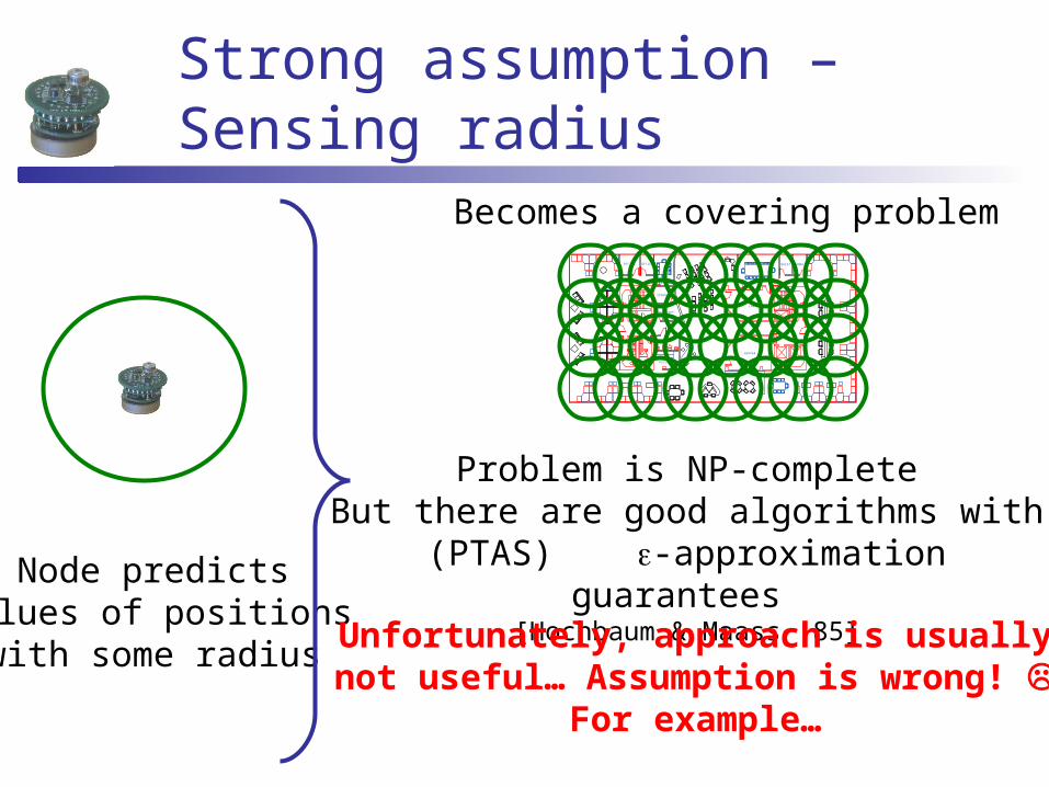
Strong assumption – Sensing radius
Node predictsvalues of positionswith some radius
Becomes a covering problem
SERVER
LAB
KITCHEN
COPYELEC
PHONEQUIET
STORAGE
CONFERENCE
OFFICEOFFICE
Problem is NP-completeBut there are good algorithms with
(PTAS) -approximation guarantees [Hochbaum & Maass ’85]
Unfortunately, approach is usually not useful… Assumption is wrong!
For example…
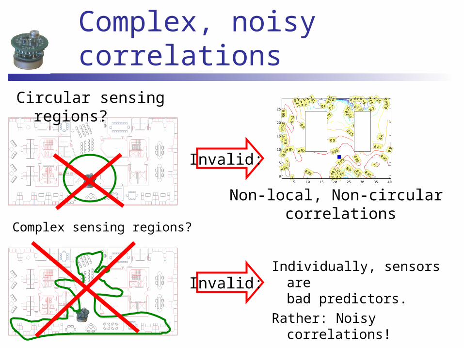
Complex, noisy correlations
Non-local, Non-circular correlations
0.5
0.50.55
0.55
0.55
0.6
0.6
0.6
0.6
0.65
0.6
5
0.6
5
0.65
0.65
0.7
0.7
0.7
0.7
0.70
.7
0.7
5
0.75
0.75
0.75
0.75
0.75
0.7
5
0.8
0.80.8
0.8
0.8
0.8
0.8
0.8
0.8
5
0.850.85
0.85
0.8
5
0.85
0.8
5
0.8
50.
85
0.9
0.9
0.9
0.9 0.9
0.9 0.9
0.9
0.9
0.95
0.95
0.95
0.950.950.95
0.95
0.95
0.9
5
0.9
5
0.9
5
0.95
1
1
1
1
5 10 15 20 25 30 35 40
0
5
10
15
20
25
Invalid:
Individually, sensors are bad predictors.
Rather: Noisy correlations!
Circular sensing regions?
Complex sensing regions?
Invalid:
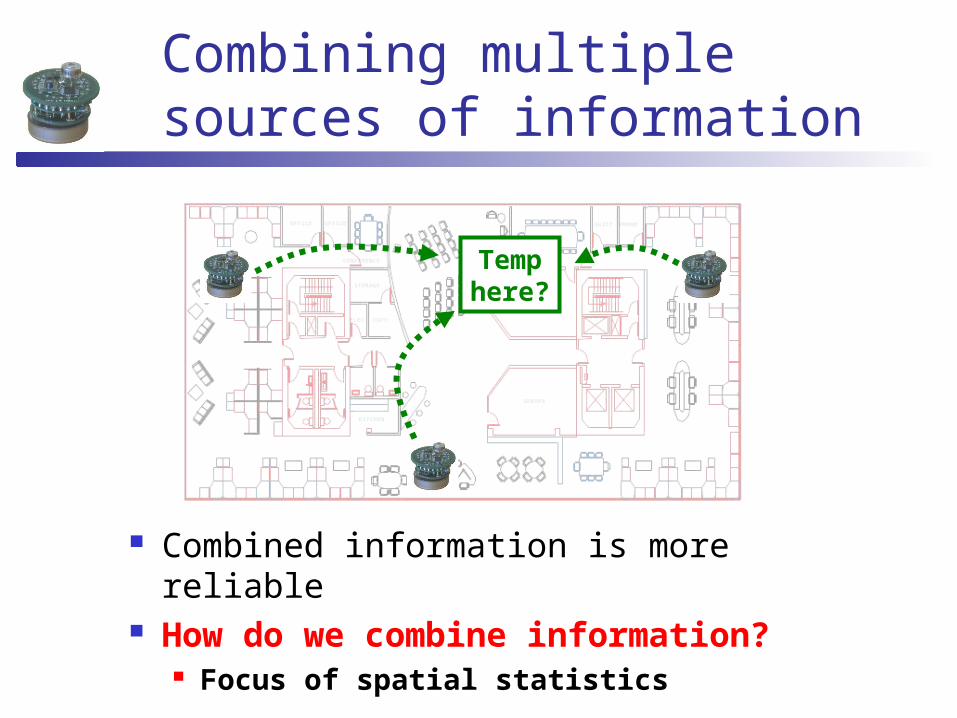
Combining multiple sources of information
Combined information is more reliable How do we combine information?
Focus of spatial statistics
Temphere?
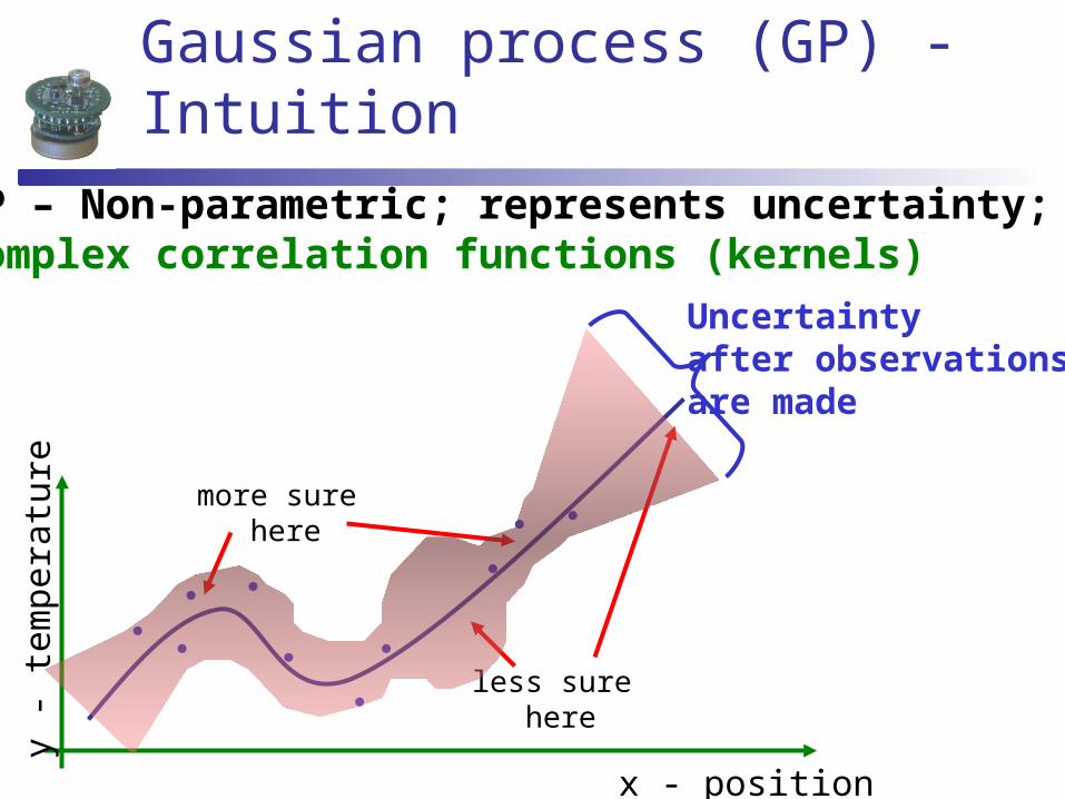
Gaussian process (GP) - Intuition
x - position
y -
tem
pera
ture
GP – Non-parametric; represents uncertainty;complex correlation functions (kernels)
less sure here
more sure here
Uncertainty after observations are made
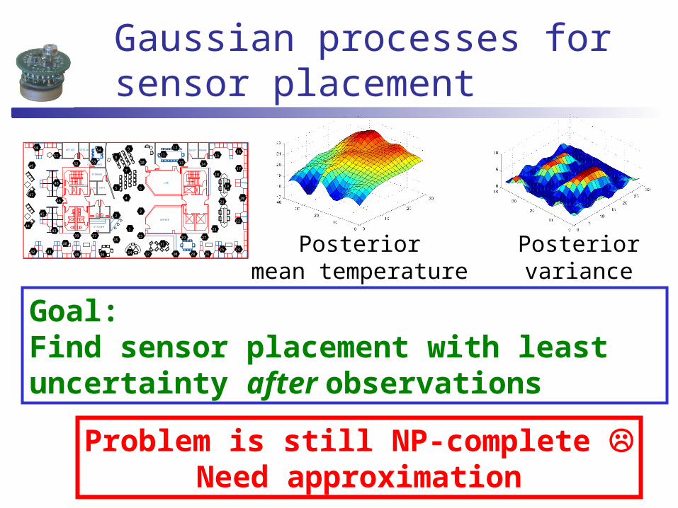
Gaussian processes for sensor placement
SERVER
LAB
KITCHEN
COPYELEC
PHONEQUIET
STORAGE
CONFERENCE
OFFICEOFFICE50
51
52 53
54
46
48
49
47
43
45
44
42 41
3739
38 36
33
3
6
10
11
12
13 14
1516
17
19
2021
22
242526283032
31
2729
23
18
9
5
8
7
4
34
1
2
3540 Posterior
mean temperaturePosteriorvariance
Goal: Find sensor placement with least uncertainty after observations
Problem is still NP-complete Need approximation
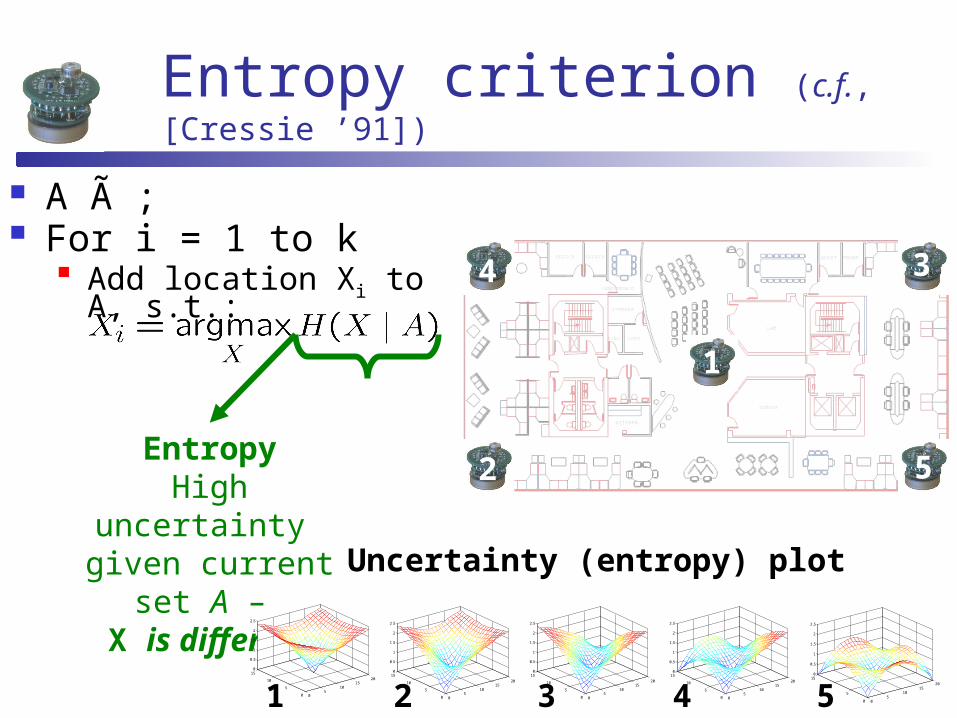
Entropy criterion (c.f., [Cressie ’91])
A Ã ; For i = 1 to k
Add location Xi to A, s.t.:
EntropyHigh uncertainty given current set
A – X is different
1
3
2
4
5
05
1015
20
0
5
10
150
0.5
1
1.5
2
2.5
05
1015
20
0
5
10
150
0.5
1
1.5
2
2.5
05
1015
20
0
5
10
150
0.5
1
1.5
2
2.5
05
1015
20
0
5
10
150
0.5
1
1.5
2
2.5
05
1015
20
0
5
10
150
0.5
1
1.5
2
2.5
Uncertainty (entropy) plot
1 2 3 4 5
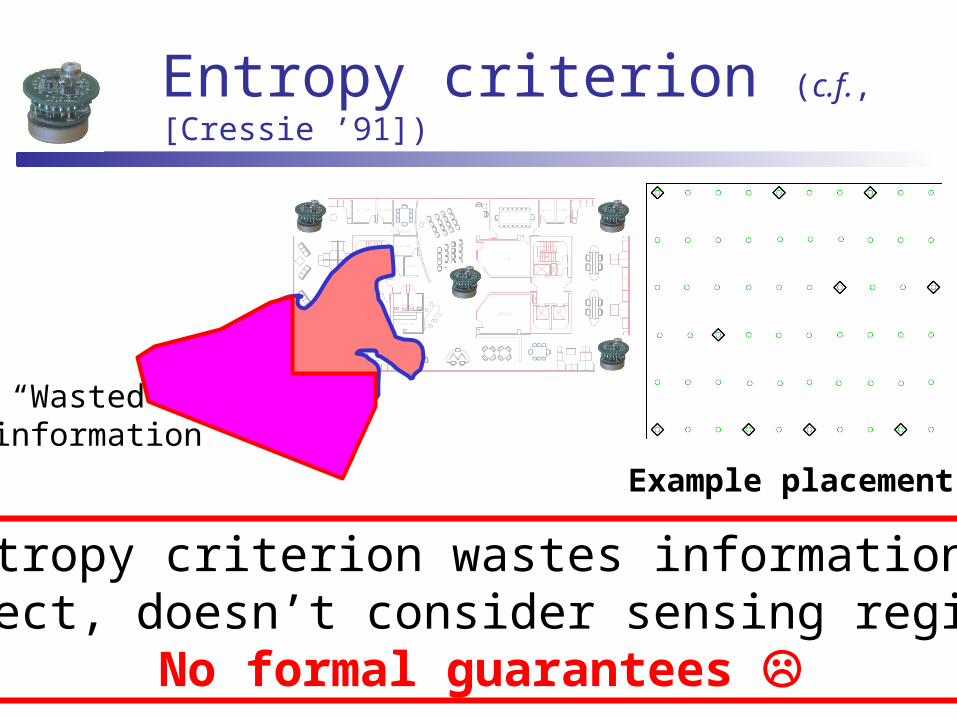
“Wasted” information
Entropy criterion (c.f., [Cressie ’91])
Entropy criterion wastes information, Indirect, doesn’t consider sensing region –
No formal guarantees
Example placement
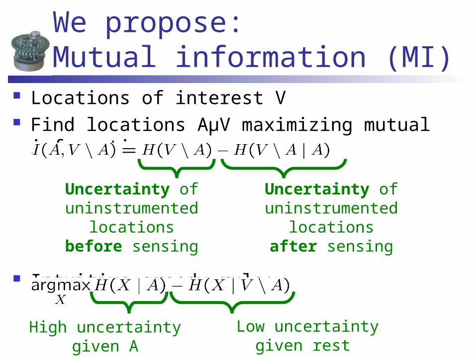
We propose: Mutual information (MI)
Locations of interest V Find locations AµV maximizing mutual
information:
Intuitive greedy rule:
High uncertainty given A
X is different
Low uncertainty given rest
X is informative
Uncertainty ofuninstrumented
locationsafter sensing
Uncertainty ofuninstrumented
locationsbefore sensing
Mutual information
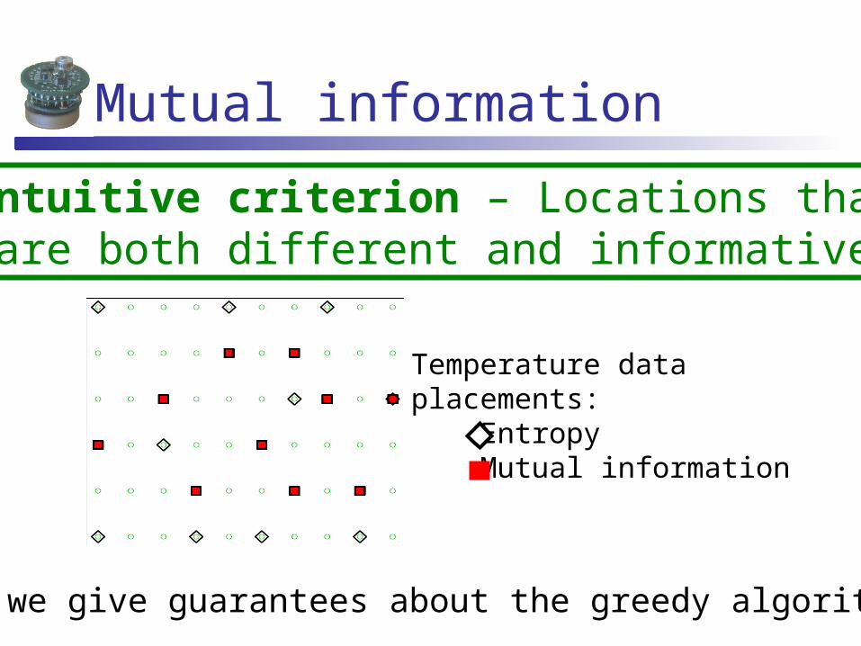
Intuitive criterion – Locations thatare both different and informative
Temperature data placements: Entropy Mutual information
Can we give guarantees about the greedy algorithm?
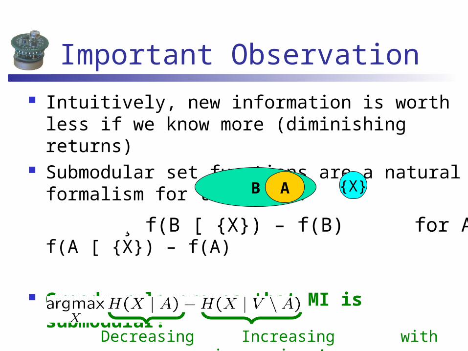
Important Observation Intuitively, new information is worth less if
we know more (diminishing returns) Submodular set functions are a natural
formalism for this idea:
f(A [ {X}) – f(A)
Greedy rule proves that MI is submodular!
B A {X}
¸ f(B [ {X}) – f(B) for A µ B
Decreasing Increasing with increasing A
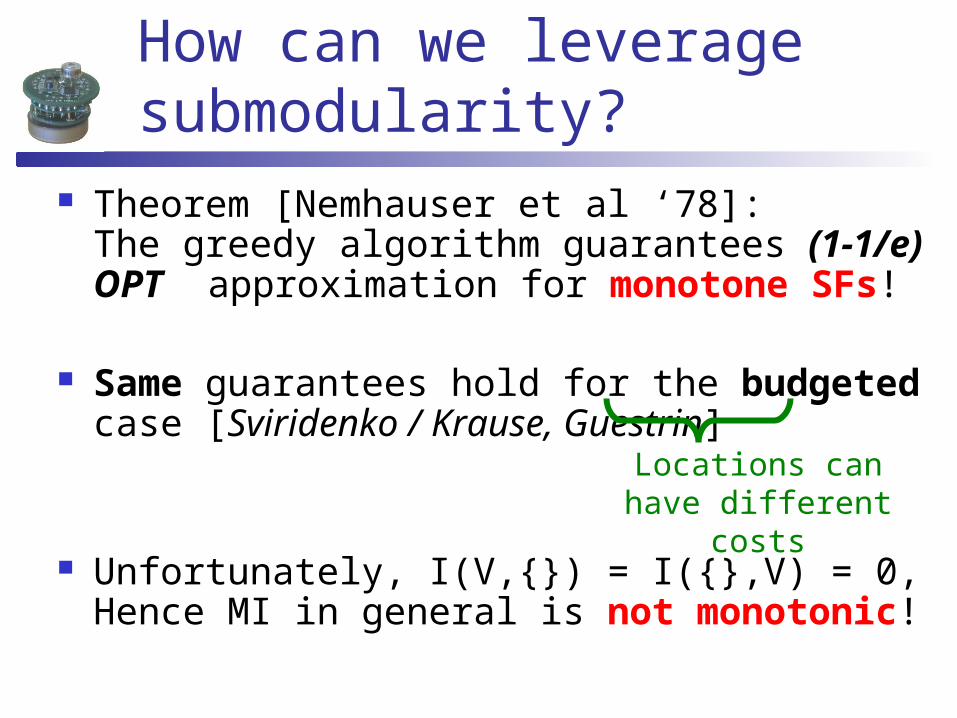
How can we leverage submodularity?
Theorem [Nemhauser et al ‘78]: The greedy algorithm guarantees (1-1/e) OPT approximation for monotone SFs!
Same guarantees hold for the budgeted case [Sviridenko / Krause, Guestrin]
Unfortunately, I(V,{}) = I({},V) = 0,Hence MI in general is not monotonic!
Locations can have different
costs
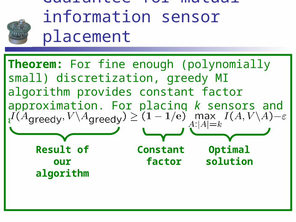
Theorem: For fine enough (polynomially small) discretization, greedy MI algorithm provides constant factor approximation. For placing k sensors and >0:
Guarantee for mutual information sensor placement
Optimalsolution
Result ofour
algorithm
Constant factor
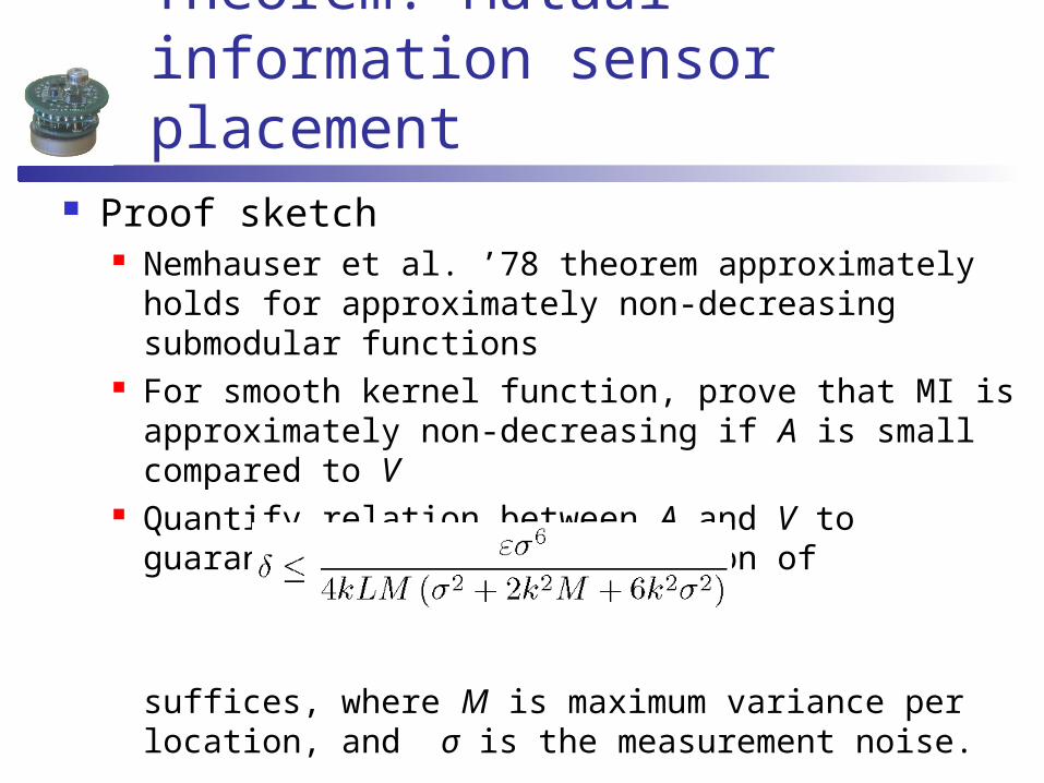
Theorem: Mutual information sensor placement
Proof sketch Nemhauser et al. ’78 theorem approximately holds
for approximately non-decreasing submodular functions
For smooth kernel function, prove that MI is approximately non-decreasing if A is small compared to V
Quantify relation between A and V to guarantee that a discretization of
suffices, where M is maximum variance per location, and σ is the measurement noise.
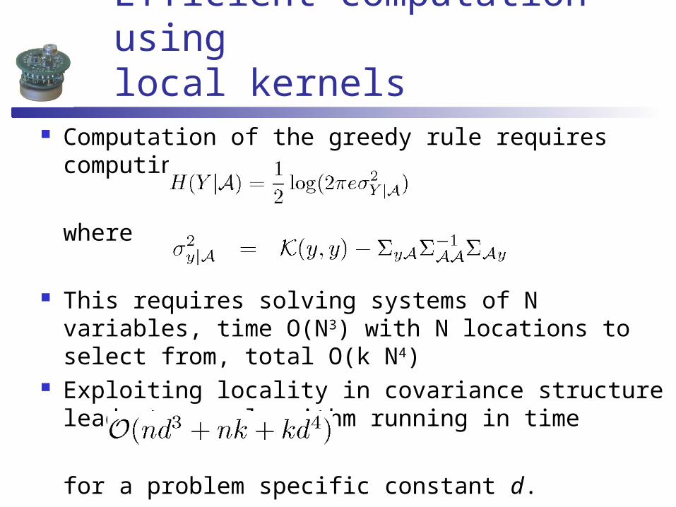
Efficient computation usinglocal kernels
Computation of the greedy rule requires computing
where
This requires solving systems of N variables, time O(N3) with N locations to select from, total O(k N4)
Exploiting locality in covariance structure leads to an algorithm running in time
for a problem specific constant d.
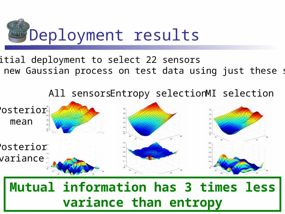
Deployment resultsUsed initial deployment to select 22 sensorsLearned new Gaussian process on test data using just these sensors
MI selection
Mutual information has 3 times less variance than entropy
Posteriormean
Posteriorvariance
All sensors Entropy selection
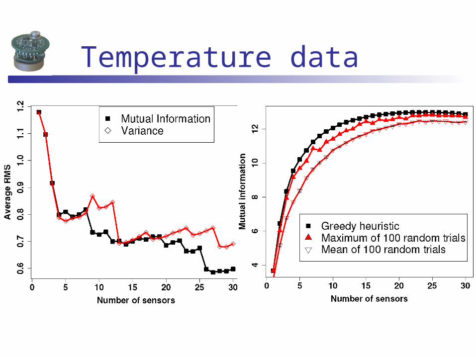
Temperature data
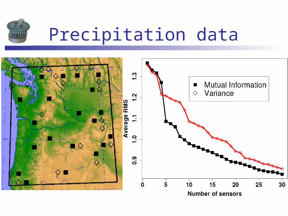
Precipitation data
Summary of Results Proposed mutual information criterion for
sensor placement in Gaussian processes Exact maximization is NP-hard Efficient algorithms for maximizing MI
placements, strong approximation guarantee (1-1/e) OPT-ε
Exploitation of local structure improves efficiency
Compared to commonly used entropy criterion,MI placements provide superior prediction accuracy for several real-world problems.