SensorlessscalarandvectorcontrolofasubseaPMSMpublications.lib.chalmers.se/records/fulltext/183931/183931.pdf · Master s Thesis 2005:22. ... This thesis deals with the position-sensorless

Improving landfill monitoring programswith the aid of geoelectrical - imaging techniquesand geographical information systems Master’s Thesis in the Master Degree Programme, Civil Engineering

KEVIN HINE

Department of Civil and Environmental Engineering Division of GeoEngineering Engineering Geology Research GroupCHALMERS UNIVERSITY OF TECHNOLOGYGöteborg, Sweden 2005Master’s Thesis 2005:22

.

Sensorless scalar and vector control of a subsea PMSM

Master of Science Thesis

Dimitrios Stellas

Department of Energy and EnvironmentDivision of Electric Power EngineeringChalmers University of TechnologyGoteborg, Sweden, 2013

THESIS FOR THE DEGREE OF MASTER OF SCIENCE


Dimitrios Stellas

Performed at: Chalmers University of Technology,Goteborg, Sweden,FMC Kongsberg Subsea,Asker, Norway

Examiner: Professor Torbjorn ThiringerDepartment of Energy and EnvironmentDivision of Electric Power EngineeringChalmers University of TechnologyGoteborg, Sweden

Supervisor: Torbjørn StrømsvikFMC Kongsberg SubseaAsker, Norway

Department of Energy and EnvironmentDivision of Electric Power Engineering

Chalmers University of TechnologyGoteborg, Sweden, 2013

i


Dimitrios Stellas

c©Dimitrios Stellas, 2013

Department of Energy and EnvironmentDivision of Electric Power EngineeringChalmers University of TechnologySE - 412 96 Goteborg, SwedenTelephone: +46 (0) 31-772 1000

Chalmers Bibliotek, ReproserviceGoteborg, Sweden, 2013

ii

Abstract

This thesis deals with the position-sensorless control of a subsea PMSM, which is fedby a remote VSD. Two V/f control alternatives are implemented for the startup of thePMSM and a sensorless vector controller is designed for operation at higher speeds.

Several simulations are performed, in order to investigate the performance of the imple-mented models and to determine the optimal control settings. The conclusions drawnfrom the simulation results are validated with measurements on a lab model.

The obtained results demonstrate that the implemented V/f control schemes can providesecure startup for the PMSM. The smoothness of the startup depends on the initial rotorposition and on the load of the motor. One of the two V/f controllers accelerates thePMSM with significantly lower current, thanks to its ability to produce a more precisevoltage reference.

During vector-controlled operation, maximum efficiency can be achieved and the responseof the system to load disturbances is almost ideal. Furthermore, the implemented field-weakening algorithm can extend the speed range of the PMSM by up to 17.6% for theconsidered load.

Index terms: PMSM, sensorless, scalar control, vector control, V/f .

iii

Acknowledgement

First of all, I would like to express my gratitude for the workplace and the equipmentthat were provided to me by the Division of Electric Power Engineering at ChalmersUniversity of Technology.

I am grateful to my examiner at Chalmers, Professor Torbjorn Thiringer, for his valuableguidance and his insightful suggestions throughout this work.

Furthermore, I would like to thank Magnus Ellsen and Alvaro Bermejo Fernandez fortheir help with the data acquisition system and Tarik Abdulahovic for his support withsoftware issues.

I also wish to express my sincere thanks to Georgios Stamatiou for his supportive attitudeand his knowledgeable advice throughout my master studies.

The financial support provided by FMC Kongsberg Subsea and the opportunity to con-duct a part of this thesis in the company’s facilities are gratefully acknowledged.

Many thanks go to my supervisor at FMC, Torbjørn Strømsvik, for his valuable supportand guidance during this thesis.

I am also thankful to Morten Thule Hansen, whose contribution in the experimental partof this work was crucial, and Harald Bjørn Ulvestad, who kindly shared his knowledgeand previous experience on the investigated system.

I also wish to thank Ola Jemtland, Vidar Kragset and Ragnar Eretveit for some usefuland interesting technical discussions during this thesis.

Finally, I am deeply indepted to my family for their unceasing support and encourage-ment.

Dimitrios Stellas

Goteborg, 2013

.

iv

Contents

1 Introduction 1

1.1 Problem background . . . . . . . . . . . . . . . . . . . . . . . . . . . . . 1

1.2 Previous work . . . . . . . . . . . . . . . . . . . . . . . . . . . . . . . . . 2

1.3 Purpose and scope . . . . . . . . . . . . . . . . . . . . . . . . . . . . . . 2

2 Theoretical background 3

2.1 Motors for subsea applications . . . . . . . . . . . . . . . . . . . . . . . . 3

2.2 Drives for submersible motors . . . . . . . . . . . . . . . . . . . . . . . . 4

2.2.1 Placement of the drive . . . . . . . . . . . . . . . . . . . . . . . . 4

2.2.2 Effects of PWM voltage . . . . . . . . . . . . . . . . . . . . . . . 6

2.3 Control of permanent magnet motors . . . . . . . . . . . . . . . . . . . . 8

2.3.1 Scalar control . . . . . . . . . . . . . . . . . . . . . . . . . . . . . 9

2.3.2 Vector control . . . . . . . . . . . . . . . . . . . . . . . . . . . . . 9

2.3.3 Combination of scalar and vector control . . . . . . . . . . . . . . 10

3 System description 11

3.1 Permanent magnet synchronous motor . . . . . . . . . . . . . . . . . . . 12

3.1.1 Electrical equations . . . . . . . . . . . . . . . . . . . . . . . . . . 12

3.1.2 Mechanical equations . . . . . . . . . . . . . . . . . . . . . . . . . 13

3.2 Transmission system . . . . . . . . . . . . . . . . . . . . . . . . . . . . . 14

3.2.1 Simplifying assumptions . . . . . . . . . . . . . . . . . . . . . . . 14

3.2.2 Considerations on transformer saturation . . . . . . . . . . . . . . 14

3.2.3 Introduction of equivalent quantities . . . . . . . . . . . . . . . . 15

3.3 Open-loop V/f control . . . . . . . . . . . . . . . . . . . . . . . . . . . . 16

3.3.1 Basic idea of the V/f controller . . . . . . . . . . . . . . . . . . . 16

3.3.2 Necessity of low initial frequency . . . . . . . . . . . . . . . . . . 17

3.3.3 Voltage boosting at low speeds . . . . . . . . . . . . . . . . . . . 17

3.3.4 Simplifying assumption . . . . . . . . . . . . . . . . . . . . . . . . 18

3.3.5 Implementation of the controller . . . . . . . . . . . . . . . . . . . 18

3.4 Closed-loop V/f control . . . . . . . . . . . . . . . . . . . . . . . . . . . . 20

3.4.1 Voltage reference calculation . . . . . . . . . . . . . . . . . . . . . 20

3.4.2 Need for stabilization . . . . . . . . . . . . . . . . . . . . . . . . . 21

3.4.3 Basic idea of the stabilizer . . . . . . . . . . . . . . . . . . . . . . 22

3.4.4 Implementation of the stabilizer . . . . . . . . . . . . . . . . . . . 22

3.4.5 Structure of the controller . . . . . . . . . . . . . . . . . . . . . . 23

v

3.4.6 Comments on the controller . . . . . . . . . . . . . . . . . . . . . 25

3.5 Vector control with position sensor . . . . . . . . . . . . . . . . . . . . . 25


3.5.2 Need for constant torque reference . . . . . . . . . . . . . . . . . 27

3.5.3 Current reference calculation . . . . . . . . . . . . . . . . . . . . . 27

3.5.4 Transfer function of the controlled system . . . . . . . . . . . . . 28

3.5.5 Inclusion of compensating terms . . . . . . . . . . . . . . . . . . . 28

3.5.6 Design of the PI regulator . . . . . . . . . . . . . . . . . . . . . . 30

3.5.7 Implementation of voltage and current limiters . . . . . . . . . . . 31

3.6 Position-sensorless vector control . . . . . . . . . . . . . . . . . . . . . . 32

3.6.1 Necessity of eliminating the position sensor . . . . . . . . . . . . . 33

3.6.2 Review of position estimation methods . . . . . . . . . . . . . . . 34


3.6.4 Implementation of the position estimator . . . . . . . . . . . . . . 36

3.6.5 Basic idea of field-weakening . . . . . . . . . . . . . . . . . . . . . 40

3.6.6 Overvoltage risk during field-weakening . . . . . . . . . . . . . . . 41

3.6.7 Field-weakening capability of the system . . . . . . . . . . . . . . 41

3.6.8 Derivation of the field-weakening algorithm . . . . . . . . . . . . . 43

4 Simulation results 45


4.1.1 Different critical frequency values . . . . . . . . . . . . . . . . . . 46

4.1.2 Different frequency reference slopes . . . . . . . . . . . . . . . . . 55

4.1.3 Different initial rotor positions . . . . . . . . . . . . . . . . . . . . 60

4.1.4 Response to load steps . . . . . . . . . . . . . . . . . . . . . . . . 63


4.2.1 Different frequency reference slopes . . . . . . . . . . . . . . . . . 65

4.2.2 Different initial rotor positions . . . . . . . . . . . . . . . . . . . . 69



4.3.1 Control transition . . . . . . . . . . . . . . . . . . . . . . . . . . . 76


4.3.3 Startup performance . . . . . . . . . . . . . . . . . . . . . . . . . 81




4.4.3 Field-weakening performance . . . . . . . . . . . . . . . . . . . . 91

5 Experimental results 97

5.1 Experimental setup . . . . . . . . . . . . . . . . . . . . . . . . . . . . . . 97

5.1.1 Small-scale laboratory model . . . . . . . . . . . . . . . . . . . . . 98

5.1.2 Control and monitoring system . . . . . . . . . . . . . . . . . . . 100

5.2 V/f control . . . . . . . . . . . . . . . . . . . . . . . . . . . . . . . . . . 101

5.2.1 Startup performance . . . . . . . . . . . . . . . . . . . . . . . . . 101

vi

5.2.2 Steady-state operation . . . . . . . . . . . . . . . . . . . . . . . . 106




5.3.3 Reversal of rotation . . . . . . . . . . . . . . . . . . . . . . . . . . 113

6 Conclusions 115





6.5 Future work . . . . . . . . . . . . . . . . . . . . . . . . . . . . . . . . . . 118

vii

List of symbols List of subscripts

ac Bandwidth of current controller 0 Initial value

cl Stabilizer gain constant a Phase-a quantity

e Back-EMF aw Anti-windup

f Electrical frequency b Phase-b quantity

Fb Voltage-boosting factor c Phase-c quantity

i Current C Cable parameter

J Moment of inertia comp Compensating value

k Gain cor Corrected value

kl Proportional gain of stabilizer cr Critical value

L Inductance d Direct-axis quantity

nr Mechanical speed (rpm) e Electrical quantity

np Number of pole pairs est Estimated value

pe Electric power gen Generator

R Resistance i Integral

Ra Active-damping resistance lim Limited quantity

t Time m Mechanical quantity

tr Rise time max Maximum value

Te Electromagnetic torque p Proportional

TL Load torque pr Predicted value

Ts Sampling period q Quadrature-axis quantity

u Voltage r Rotor quantity

θ Transformation angle rated Rated value

κ Sampling number s Stator quantity

φ Angular position T Transformer parameter

φ0 Power factor angle tr Transmission system parameter

ψ Flux linkage upd Updated value

Ψm Flux linkage of magnets

ω Electrical speed

Ω Mechanical speed

List of abbreviations List of superscripts

AC Alternating Current ∗ Reference quantity

DC Direct Current ′ Equivalent quantity

EMF Electromotive Force s Stationary-frame vector

HPF High-Pass Filter

IMC Internal Model Control

LC Inductive-Capacitive List of accentsLPF Low-Pass Filter

MTPA Maximum Torque Per Ampere ˆ Peak value

PI Proportional-Integral ¯ Space vector

PMSG Permanent Magnet Synchronous Generator

PMSM Permanent Magnet Synchronous Motor

PWM Pulse-Width Modulation

RL Resistive-Inductive

V SD Variable Speed Drive

viii

Chapter 1

Introduction

This chapter introduces the problem that is addressed in this thesis, presents some pre-vious work that has been conducted on the investigated system and states the scope andthe objectives of this thesis.

1.1 Problem background

Induction motors are the most traditional option for driving submersible pumps. How-ever, as the oil production moves to deeper waters, it becomes necessary to consideralternatives that can facilitate higher performance.

PMSMs have the potential to meet the emerging challenges in subsea applications, thanksto positive features such as high efficiency, high power density and high-speed capabilities.

The VSDs that are used for the control of submersible PMSMs are often installed onoil platforms, which can be located several kilometers away from the subsea pumpingactivities. The long eletrical connection between the motor and the drive in these casesintroduces new challenges in the control of the PMSM.

Although the control requirements of pump drives are usually low, the recent develop-ment of advanced pumping solutions calls for more efficient and precise motor regulation.

The new performance demands can be met by vector control, a control type which isusually applied in advanced drive systems, which require fast and accurate current andspeed regulation. Typical examples of applications that use vector control can be foundwithin the automotive industry.

The harsh operating conditions imposed by the deepwater environment of submersiblePMSMs necessitate the sensorless operation of the applied control schemes. This meansthat the used vector controllers must not rely on mechanical measurements, but shouldhave position-estimating capabilities.

Since the performance of position-sensorless vector control is usually problematic duringthe startup of the PMSM, a more traditional control type, called scalar control, can beused during the low-speed operation of the system.

1

1.2 Previous work

The offshore system considered in this thesis consists of a submersible motor, which isremotely controlled by a VSD through a transmission system. The transmission systemconsists of a step-up transformer, a long cable and a step-down transformer.

A small-scale lab model of this system was designed and implemented as part of a pre-vious work [1]. Computer simulations were also performed during the same work, inorder to study the startup performance of the downscaled system under scalar control.A separate task included the setup of the scalar and vector control configurations in theVSD of the lab model.

Since the measurements that are presented in this thesis were taken on the small-scale labmodel and since the aforementioned drive configurations were used to control the PMSMduring the performed experiments, it is clear that the experimental tasks performed inthis thesis are based on previously conducted work.

The control schemes implemented in this thesis are mainly based on concepts that havebeen found in literature. The designed models have resulted from the combination ofideas from different papers and the adaptation of these ideas to the peculiarities of theinvestigated system.

1.3 Purpose and scope

The first objective of this thesis is to develop sensorless scalar and vector control modelsfor the studied system and to simulate their performance both during the startup andduring high-speed operation of the PMSM. The modeling and the simulations are per-formed with MATLAB and Simulink.

Since this work focuses on the development of control schemes, the modeling of thephysical components is not handled in detail. The PMSM model is obtained from theSimPowerSystems toolbox and the transmission system parameters are integrated intothe motor parameters. The VSD and its output filter are represented by a simplifiedinterface between the control circuit and the power circuit.

The second objective of this thesis is to verify the results of the simulations with measure-ments on the lab model of the system. The preparation for these measurements includesthe development of a data-acquisition system, which can be used to monitor differentquantities during the conducted experiments. The implemented monitoring system isbased on LabVIEW and CompactRIO.

2

Chapter 2

Theoretical background

This chapter presents some theoretical considerations that are related to the studied sys-tem. The increasingly important role of PMSMs for subsea operations is discussed anddifferent options for the placement of drives in offshore applications are presented.

In cases where the submersible motor is controlled by a remote VSD, the combination ofthe PWM voltage output of the drive and the long cable connection between the motorand the drive introduces certain challenges, which are discussed in this chapter.

Finally, some theoretical background about the sensorless scalar and vector control ofPMSMs is presented and the combination of these two control types is introduced, asa way to achieve safe motor startup and high control performance during high-speedoperation.

2.1 Motors for subsea applications

PMSMs have positive features that make them popular in a variety of applications. Whenit comes to deepwater pumping operations, the advantages of PMSMs become even moresignificant, as explained in this section.

Due to the high deepwater pressures involved, subsea motors typically operate with fluid-filled mechanical gaps. The presence of pressurized fluid between the rotor and the statorhelps the motor withstand the high pressure of its subsea surroundings, but also resultsin increased friction and causes higher drag losses, compared to the case of air-filled gaps.

Whereas the electrical losses are dominant in conventional motors with air-filled gaps,this is not the case for motors that operate subsea. The highly effective cooling that isavailable in subsea applications makes the impact of the electrical losses less significant,compared to that of frictional losses [2].

A typical breakdown of the total losses in this case shows that approximately 70% ofthem are drag losses, almost 20% are losses from the impeller which circulates the fluidand only 10% are electrical losses [3].

Apparently, the high drag losses pose severe limitations in the operating speed of motors

3

with fluid-filled gaps. Since high speeds are increasingly important for subsea pumpingapplications [2], it is crucial to decrease the frictional losses in submersible motors.

Induction motors have been traditionally used in subsea applications, thanks to their sim-plicity, robustness and low cost. However, as the oil production moves to deeper waters[4], it becomes harder for them to meet the increased speed and efficiency requirements,mainly because their need for a small mechanical gap results in high frictional losses.

PMSMs on the other hand, can be constructed with much larger mechanical gaps, whichresults in higher efficiency and greater speed capabilities. Their decreased sensitivity tolarger gaps allows smaller rotor diameters and extra space for the placement of a sleevein the fluid-filled gap of the motor [2].

Additionally, the absence of rotor windings or conductive bars in PMSMs eliminates theresistive rotor losses. This allows even higher efficiencies and superior thermal perfor-mance compared to induction motors.

Apart from their high efficiency and high speed capabilities, PMSMs are characterizedby high power density, compact size and low weight [5, 6]. Their construction is simpleand the absence of brushes results in higher robustness and lower maintenance needs [7].

On the negative side, the high cost of the permanent magnets increases the overall costof PMSMs [8]. Moreover, the risk of magnetic property loss makes the reliability of thismotor type questionable under certain circumstances [6].

2.2 Drives for submersible motors

The use of VSDs for the control of submersible motors improves the reliability and theefficiency of pumping operations.

This section presents different options regarding the placement of the drive and discussessome problematic issues that arise from the combination of the PWM voltage generatedby the VSD and the long cable that connects the motor and the drive.

2.2.1 Placement of the drive

The VSDs that are used for the control of submersible motors can be placed either onthe seabed, in the vicinity of the controlled motor [9], or on a platform, which might belocated several kilometers away from the actual pumping activity [10, 11].

Placement in low-pressure subsea enclosures

In the first case, the drive is enclosed in a vessel, which is installed subsea. Since powerelectronic converters that are based on present technology cannot withstand high-pressureenvironments, the interior of the drive vessel needs to be at low pressure [12].

4

Due to the high deepwater pressure, the drive enclosure in this case must be able to with-stand a significant pressure difference between its interior and its subsea surroundings.For this reason, the walls of the used vessel need to be thick and heavy.

Naturally, the bulky design of the enclosure results in an increase in the size and cost ofthe drive system, but also in problematic heat dissipation [12]. Due to the thick walls ofthe vessel, the heat conduction from the power electronic components to the sea waterbecomes more difficult, which results in higher operating temperatures for the drive.

Placement on the platform

The second option is to install the converter on a platform. Although the topside envi-ronment eliminates the necessity of a large and costly enclosure, it introduces the needfor a long electrical connection between the VSD and the controlled PMSM [10, 11].

In order to decrease the transferred current and thus reduce the transmission losses andthe voltage drop in the cable connection, higher transmission voltage levels are neededfor longer step-out lengths. For this reason, a topside transformer can be used to step upthe voltage output of the VSD.

In this case, either the submersible PMSM needs to operate at the voltage levels of thetransmission system [1], or an additional transformer needs to be installed on the seabed,so that the transmitted voltage can be stepped down before reaching the motor. In theframework of this thesis, the latter alternative is considered.

A potential drawback of this solution is that the control of the PMSM through thetransmission system could introduce new filtering requirements [13]. More specifically,the transmission of the PWM pulses of the drive through the long cable could subjectthe windings of the PMSM to significant electrical stress, if the necessary measures arenot taken. This issue is discussed in greater detail in Section 2.2.2.

Development of pressure-tolerant power electronics

The development of pressure-tolerant power electronics could facilitate the possibility ofplacing the drive in subsea enclosures of reasonable size and cost. The vessel in thiscase could be filled with a pressurized insulating liquid, which would improve the heatdissipation and would eliminate the differential pressure that the vessel would otherwisehave to withstand.

The insulating liquid must protect the converter components from mechanical damageand electrical flashovers. It should have good dielectric and thermal properties, in orderto provide reliable insulation and effective heat removal. It should be uncompressibleand should have a uniform and stable structure, which would not cause any chemicalreactions or change its character for any reason [12, 14].

A dielectric liquid, which has been tested for the described purpose and appears to haveseveral desirable features, is Midel 7131. Its properties include high breakdown strength,low thermal expansion, high temperature stability, biodegradability and non-toxicity [14].

5

A strategy that has been proposed for the development of power electronic componentsthat could withstand the high pressure of the insulating liquid is the removal of the in-sulating gas that originally surrounds the converter chips and its replacement with anuncompressible liquid. This liquid should ideally fill every void in the converter [12].

Although the development of pressure-tolerant power electronics could enable the place-ment of the VSD in high-pressure submersible enclosures in the future, such a solution isnot an option for present applications.

2.2.2 Effects of PWM voltage

The PWM voltage produced by the topside VSD is transmitted through the cable to thesubmersible PMSM. The high-frequency voltage pulses generated by the inverter couldhave detrimental effects on the motor and the cable.

As discussed in this section, the effects of the PWM voltage may be quite severe in the in-vestigated application, due to the long transmission distance and the subsea environmentof the cable.

Impact of high-order harmonics

Compared to a purely sinusoidal voltage excitation, the PWM pulses that are suppliedto the motor result in increased losses, mechanical vibrations, noise generation, higherelectromagnetic emission, more severe insulation stress, and undesirable currents inducedto the shaft and bearings of the motor [15, 16].

The high-order harmonics of the PWM voltage induce high-frequency currents and thuscreate minor hysteresis loops in the steel of the motor. These currents are the cause ofadditional losses, which reduce the efficiency of the system and result in higher operatingtemperatures. Furthermore, the interaction of the induced currents with flux harmonicsmay result in stray forces that cause mechanical vibrations and increase the generatednoise [15].

Increasing the switching frequency of the drive is a way to reduce the harmonic contentof the motor currents and thus mitigate the negative effects of the high-frequency currentcomponents. However, this also results in higher switching losses in the drive and increasesthe possibility of voltage overshoots in the motor terminals [17].

Voltage overshoots at the terminals of the motor

The high-frequency voltage pulses generated by the VSD cause travelling waves in thetransmission cable between the drive and motor. When each travelling wave reaches thePMSM, voltage reflection occurs, due to the mismatch between the cable impedance andthe motor impedance [18].

The magnitude of the reflected voltage depends on the cable length, the rise time of thepulses, the characteristic impedances of the motor and the cable, the propagation velocity

6

of the waves and the dielectric medium surrounding the cable [13].

Shielded cables and cables that are submersed in water have significantly higher capaci-tance than cables in air. This results in lower characteristic impedances for submersiblecables and therefore a more significant mismatch between the cable impedance and themotor impedance [13].

Since the impedance of the motor is much higher than the one of the cable, the reflectedwave is expected to be almost equal in magnitude to the incident wave. Since the voltageat the motor terminals is equal to the sum of the two waves, its magnitude is expectedto reach twice the magnitude of the VSD voltage [19].

Due to the occuring voltage reflection phenomena, when the distance between the motorand the drive is long, as in the case of the investigated application, the voltage pulses atthe motor terminals may be different than the ones generated by the drive.

More specifically, the distributed inductance and capacitance of the cable result in high-frequency voltage oscillations at the motor end of the cable. These oscillations are usuallyreferred to as ’voltage ringing’ [18].

Moreover, the high voltage derivatives experienced by the PMSM during PWM operationcause the voltage peaks to be unevenly distributed across the motor windings. In thiscase, the largest portion of the supplied voltage may appear between the first turns ofthe windings, thus causing the insulation of these turns to experience higher stress andfaster degradation [17].

It can be concluded that the combination of voltage reflection and voltage ringing cancause the motor to experience voltages higher than twice the DC-link voltage of the VSD[17], while the high voltage derivatives can subject the motor windings to additional elec-trical stress.

If these phenomena are not taken into account during the design of the system, therepeated overvoltages can cause significant stress to the insulation of the motor andeventually reduce its lifetime.

Cable-charging current pulses

Every time the voltage output of the VSD changes, the distributed cable capacitancemust be charged or discharged. This results in pulses of charging current that not onlyincrease the losses of the system, but can also cause overcurrent problems in the inverterand affect the control performance of the drive [18].

The magnitude of the charging current is proportional to the derivative of the voltagesupplied by the drive and to the cable capacitance. Since PWM pulses are characterizedby rapid voltage variations and since the capacitance of submersible cables is large, thecharging currents are expected to be high in the investigated application.

7

The frequency of the cable-charging current pulses depends on the frequency of the voltagepulses generated by the inverter. Therefore, for higher switching frequencies of the VSD,the distributed cable capacitance is charged and discharged more often, which increasesthe transmission losses of the system.

Mitigation of the PWM effects

Based on the aforementioned considerations, the combination of PWM operation and thelong cable connection between the VSD and the PMSM can potentially cause significantstress to the insulation of the motor and decrease the efficiency of the system.

These negative issues can be mitigated by filtering the voltage that is generated by theVSD, or by eliminating the impedance mismatch at the end of the cable. There are dif-ferent types of filters that can be used for these purposes, the most common ones beingoutput line inductors, output limit filters, sine wave output filters and motor terminationfilters [18]. The cost and the effectiveness of the aforementioned solutions vary.

The use of sine wave filters has been suggested in several papers [13, 16, 19], as a way toeliminate the high-order harmonics of the PWM pulses and therefore supply the motorwith almost sinusoidal voltage.

The advantages of this solution include the absence of transient overvoltages at the termi-nals of the motor, the elimination of power losses due to harmonic currents, the reductionof motor noise and the decrease of electromagnetic emission [19].

Moreover, when applications with submersible motors and long step-out distances areconsidered, the use of sine wave filters is expected to eliminate the negative phenomenathat are associated with voltage reflection and high voltage derivatives [13].

A sine wave filter is essentially a LC filter, whose resonance frequency is much lowerthan the lowest harmonic frequency of the inverter voltage and much higher than thefundamental frequency of the system [16].

An alternative solution, which has been introduced as an effort to eliminate the require-ment for filters, is the use of a multilevel inverter in the VSD [10]. The special topologyof this inverter results in a significant reduction in the high-order harmonics at the out-put of the drive and eliminates several problems that are associated with common PWMvoltage pulses.

2.3 Control of permanent magnet motors

Depending on the requirements of each application, different methods can be used tocontrol PMSMs. This section introduces scalar control as a simple control method, whichis suitable for low-cost drive systems, and vector control as a more advanced option, whichis well-suited for applications that demand higher dynamic performance.

8

2.3.1 Scalar control

In drive systems where simple, low-cost control is desired and where reduced dynamicperformance is acceptable, open-loop control methods can be used. Typical applicationsof such systems include pump and fan drives [20]. Open-loop control methods (or scalarcontrol methods, as they are often called) exist in different variations, which include V/fschemes [21] and I-f schemes [22].

Despite their simplicity and their ability to operate over a wide speed range, it has beenfound that the performance of open-loop methods often depends on the motor parametersand the load conditions of the system. Such methods can experience power swings withinspecific speed ranges, which might cause the motor to lose synchronism [5].

Furthermore, the behaviour of some open-loop schemes is heavily dependent on the se-lected parameters of the controller. The selection of the control settings for these schemesis often based on a trial-and-error approach and is therefore quite time-consuming [21].

The term ’open-loop’ often refers to the fact that no speed or position feedback is neededfor the operation of these schemes. In this thesis however, this term is used to denotethat neither electrical nor mechanical feedback is required by a controller.

For instance, a scalar control method which uses current feedback has been presentedin [23]. Although this method does not require any position or speed measurements,it is called ’closed-loop’ in this thesis, in order to differentiate it from schemes with nofeedback at all.

2.3.2 Vector control

For more advanced drive systems, which require higher dynamic performances, vectorcontrol is a more appropriate option than scalar control. Demanding applications thatneed vector control can be found, for instance, within the automotive industry [20].

Vector control allows the torque and the flux of the PMSM to be controlled separatelyfrom each other, through a control structure which is similar to that of a separatelyexcited DC machine [20]. This decoupled control results in the precise and efficient reg-ulation of the motor.

However, a major issue with vector controllers is that their operation requires informa-tion about the rotor position and the speed of the PMSM. The most direct approach forobtaining this information, is the use of mechanical sensors on the shaft of the PMSM [24].

In many applications however, the presence of mechanical sensors is undesirable or un-acceptable, since it increases the cost and the complexity of the system [25].

Numerous position-estimating techinques have been developed, as an effort to eliminatethe need for mechanical sensors. The position estimation can be based, among others,on the flux linkage, the back-EMF or the inductance of the PMSM [26, 27]. The effec-

9

tiveness of these techniques is not universal, but depends on the motor topology and theapplication requirements.

Several proposed vector control schemes utilize flux-linkage-based estimation techniques[5, 21]. Such a technique has been described in [26] and is implemented in this thesis,after being adapted to the peculiarities of the investigated system. Variations of theimplemented estimating algorithm have also been presented in [25, 28, 29].

Field-weakening algorithms are often integrated into vector control schemes, in orderto allow the PMSM to operate above its rated speed. Several papers have presentedtheoretical considerations on field-weakening [30, 31] and have applied different field-weakening strategies [32, 33]. A field-weakening algorithm, which has been derived in[34], is implemented and tested in this thesis.

2.3.3 Combination of scalar and vector control

A problem with most position-estimating techniques is their inability to produce accu-rate estimates at zero speed. Due to this problem, the startup of PMSMs with position-sensorless vector controllers is often problematic, unless the initial rotor position is known[29].

A solution would be to bring the rotor to a known position before the actual accelera-tion [25]. This could be achieved by injecting a proper DC current into the windings ofthe PMSM, thus forcing the rotor to align in the desired direction. For the investigatedsystem however, such a solution is not acceptable, since the presence of the transformersdoes not allow the injection of DC currents.

Due to the startup issue of position-sensorless vector controllers, scalar control schemesare often used for the initial acceleration of PMSMs [5, 22]. Provided that their controlparameters are properly set, these schemes should be able to accelerate the PMSM forevery initial rotor position [29]. After a certain speed is reached, the scalar controller canbe dismissed and the position-sensorless vector controller can be deployed.

This well-known strategy is also applied in this thesis. Two V/f control alternativesare presented for the startup of the PMSM and a position-sensorless vector controller isimplemented and tested for higher speeds of the motor. A vector control scheme withmechanical sensors is also designed, as an intermediate step before the implementationof the sensorless controller.

10

Chapter 3

System description

This chapter describes the models that have been implemented in this thesis and theconsiderations that determined their design. The described models correspond both tothe power components and the drive controller of the studied system.

The considered power system consists of a PMSM, which drives a multiphase pump andwhich is fed by a remote VSD through a transmission system. The transmission systemconsists of a step-up transformer, a long cable and a step-down transformer. The topol-ogy of the system is shown in Fig. 3.1.

Step-up

transformer

M P

VSDPower source

PMSM Multiphase

pump

Cable

Step-down

transformer

SubseaTopside

Figure 3.1: Topology of the investigated power system, consisting of a PMSM, which is con-nected to a pump and is fed by a remote VSD through a transmission system.

The controller of the VSD determines the voltage output of the drive and therefore thevoltage input of the motor. The application of proper control schemes is essential, inorder to achieve the required performance during different types of operation.

Two different V/f control models, an open-loop and a closed-loop model, are implementedfor the initial acceleration of the PMSM and are presented in this chapter. The formerone is simpler but the latter one provides higher control performance.

Moreover, two different vector control models are designed for higher operating speedsof the PMSM. In the first model a position sensor is present, while in the second modelthis sensor is eliminated, in order to decrease the cost and increase the robustness of the

11

system.

3.1 Permanent magnet synchronous motor

This section presents the equations which dictate the electrical and mechanical perfor-mance of the PMSM and provide the basis, not only for the implementation of the motormodel, but also for the design of its control.

3.1.1 Electrical equations

It is generally convenient to express the electrical equations of the PMSM in the dq ref-erence frame [35]. By using this representation, the steady-state AC quantities of themotor are transformed into DC values, which are easier to analyze and control.

The space vector of the stator voltage is denoted as us and is given by

us = Rsis +dψsdt

+ jωrψs (3.1)

where Rs is the stator resistance, is is the space vector of the stator current, ψs is thespace vector of the stator flux linkage and ωr is the electrical speed of the motor. Thestator flux linkage ψs is obtained from

ψs = Lsdisd + jLsqisq + Ψm (3.2)

where Ψm is the amplitude of the flux linkage of the permanent magnets, Lsd and Lsq arethe d-axis and q-axis stator inductances and isd and isq are the d-axis and q-axis currentsrespectively.

It can be observed from (3.2) that Ψm lies in the d direction, thus the magnetic axis ofthe PMSM is the same with the d axis of the selected dq frame. This is achieved by usinga proper angle θr for the dq tranformations.

The back-EMF of the PMSM depends on the flux linkage Ψm and the speed ωr. Its spacevector e is given by

e = jωrΨm (3.3)

By combining (3.1) and (3.2), the d-axis and q-axis stator voltages, denoted as usd andusq respectively, can be obtained as

usd = Rsisd + Lsddisddt− ωrLsqisq (3.4)

usq = Rsisq + Lsqdisqdt

+ ωrLsdisd + ωrΨm (3.5)

where the term ωrΨm represents the magnitude of the back-EMF vector e, or equiva-lently, the amplitude of the three-phase back-EMF. It is important to note that, since

12

amplitude-invariant transformations are used in this thesis, the magnitudes of space vec-tors correspond to the amplitudes of three-phase quantities.

Next, the electromagnetic torque Te of the motor can be calculated from

Te =3np2Im[ψ∗s is] =

3np2

[Ψmisq + (Lsd − Lsq)isdisq] (3.6)

where np is the number of pole pairs. The values of the inductances Lsd and Lsq dependon the geometry of the motor and the placement of the permanent magnets [8, 36].

PMSM topologies with inset-mounted or interior-radial magnets are characterized by dqsaliency, which results in a difference between Lsd and Lsq. On the other hand, in motorswith surface-mounted magnets, the saliency is often negligible and the two inductancescan be considered to be equal, thus Lsd = Lsq = Ls. In the latter case, (3.6) is simplifiedto

Te =3np2

Ψmisq (3.7)

The inductances Lsd and Lsq of the PMSM considered in this thesis differ slightly fromeach other. However, for the sake of simplicity, the difference between them is neglectedand the simplified expression (3.7) is used for the calculation of the electromagnetictorque.

It is interesting to observe that the torque in (3.7) is proportional to the current isq andindependent of isd. The current isd on the other hand, has a more significant effect onthe stator flux linkage magnitude than isq according to (3.2), since the first one lies onthe same axis with the main flux linkage component Ψm, while the second one lies on aperpendicular axis.

3.1.2 Mechanical equations

The equation that dictates the mechanical performance of the PMSM, by relating theelectromagnetic torque Te, the load torque TL and the electrical speed ωr, is

J

np

dωrdt

= Te − TL (3.8)

where J is the moment of inertia of the system. The relation between the electrical speedand the electrical rotor position is given by

dφrdt

= ωr (3.9)

where φr corresponds to the angle between the magnetic axis of the motor and the a axisof the three-phase system.

In order to achieve perfect-field orientation, thus in order to align the magnetic axis ofthe PMSM with the d axis of the dq frame, the electrical rotor angle φr needs to be equal

13

to the selected dq-transformation angle θr, thus φr = θr.

The motor model which is used in this thesis is based on the electrical equations (3.4) -(3.6) and the mechanical equations (3.8) - (3.9).

3.2 Transmission system

The transmission system in the studied application consists of a step-up transformer, acable and a step-down transformer. In order to reduce the computational complexityof the simulations and to simplify the selection of the control settings, the electricalparameters of the transmission components are integrated into the respective parametersof the PMSM.

3.2.1 Simplifying assumptions

The aforementioned treatment of the transmission system is facilitated by two basic as-sumptions.

Firstly, it is assumed that the short-line model can represent the cable of the systemwith adequate accuracy, thus the shunt capacitance of the cable can be ignored, withoutintroducing any significant error. Under this assumption, which is generally valid for lineswith length up to 80 km [37], the transmission cable can be modelled as an inductanceLC connected in series with a resistance RC .

Secondly, it is assumed that none of the two transformers experience saturation, thus theyare both considered to remain in the linear magnetic region under all operating conditionsof the system. Under this assumption, the magnetizing branch of their equivalent circuitcan be ignored and each transformer can be modelled as an inductance LT connected inseries with a resistance RT .

3.2.2 Considerations on transformer saturation

In general, the core of a transformer gets saturated when the applied V/f ratio becomestoo high. In such a case, the rise in the magnetic flux linkage of the transformer is accom-panied by a disproportionally large increase in its magnetizing current and, therefore, asignificant decrease in its magnetizing inductance.

Clearly, saturation is an undesirable condition for transformers and should be avoided bydimensioning their core properly, so that they remain in the linear magnetic region evenfor the maximum applied V/f ratio.

The aforementioned requirement bears particular significance for the studied application.As discussed in Section 3.3.3, the system has to operate at a high V/f ratio during theinitial stage of the PMSM startup. This may lead to the inconvenient necessity of over-sizing the transformer core for the sake of a few seconds of low-frequency operation.

14

The problem applies mainly to the topside step-up transformer, since the V/f ratio thatis experienced by the subsea step-down transformer is lower, due to the voltage drop inthe cable.

In order to minimize the size and cost of the topside transformer, it is necessary tooptimize the control of the PMSM during the early stages of its startup, thus to find theminimum V/f ratio that can safely accelerate the motor.

3.2.3 Introduction of equivalent quantities

By neglecting the shunt capacitance of the cable and the magnetizing branch of thetransformers, the transmission system can be simply modelled as a series RL circuit. Itsresistance Rtr and and its inductance Ltr can be written as

Rtr = RC + 2RT (3.10)

Ltr = LC + 2LT (3.11)

respectively. Since the transmission system is connected in series with the stator windingsof the PMSM, its parameters can be integrated into the motor parameters. In this case,the combination of the actual PMSM and the transmission system can be regarded as anequivalent PMSM, the parameters of which can be written as

R′s = Rs +Rtr (3.12)

L′s = Ls + Ltr (3.13)

where R′s is the equivalent stator resistance and L′s is the equivalent stator inductance.

The control of the actual motor through the transmission system can then be regarded asdirect control of the equivalent motor. The implemented controllers compensate for thevoltage drop in the transmission system, by considering the equivalent stator parametersR′s and L′s, an equivalent stator voltage u′s and an equivalent stator flux linkage ψ′s,whenever needed.

Having integrated the transmission system parameters into the motor parameters, theactual voltage us of the PMSM can be calculated by subtracting the voltage drop in thetransmission impedance from the equivalent voltage u′s, which is the voltage producedby the VSD. The voltage drop, in turn, can be easily obtained when the transmissionparameters Rtr and Ltr and the stator current is are known.

The system should be designed in a proper way, so that a specified steady-state voltagedrop occurs in the transmission system. In the actual application, where the transmissiondistance is fixed, this could be achieved by selecting an appropriate level for the operatingvoltage and a cable with suitable parameters.

15

In the performed simulations on the other hand, the voltage level and the transmissionsystem parameters are considered to be fixed and the desired voltage drop is obtained byselecting the proper cable length.

3.3 Open-loop V/f control

This section discusses the basic idea of V/f control, explains the need for a low startupfrequency and introduces a voltage-boosting factor for low-speed operation of the PMSM.

It also describes the implemented open-loop V/f regulator, which is deployed to acceleratethe motor from standstill up to a certain speed level. The term ’open-loop’ refers to thefact that no feedback is received by the controller and therefore no current or speedmeasurements are needed for its operation.

3.3.1 Basic idea of the V/f controller

The fundamental idea of V/f control can be demonstrated by considering (3.1) underthe assumptions that the stator flux linkage is constant and that the resistive term isnegligible. This gives

us ' jωrψs ⇒ ψs 'usωr⇒ ψs '

us2πf

(3.14)

where f is the electrical frequency and ψs and us are the magnitudes of the flux linkagevector and the voltage vector respectively, thus the amplitudes of the respective three-phase quantities.

Equation (3.14) shows that in order to keep the stator flux linkage approximately con-stant, the amplitude of the supplied stator voltage must be varied proportionally to theelectrical frequency.

With the exception of field-weakening operation, it is generally desirable to maintain thevalue of the stator flux linkage around its nominal level, which is approximately equal tothe rated voltage over the rated speed [20].

For high values of the V/f ratio, the motor becomes overexcited and a rise in the currentisd occurs, according to (3.2). A low V/f ratio on the other hand, causes the motor toexperience underexcitation, which is associated with a negative isd.

Both overexcited and underexcited states are accompanied by a rise in the stator current,as a result of the increased magnitude of its d-axis component. Since the current isd doesnot contribute to any torque production, according to (3.7), the increase of its magnitudeis translated into a rise in power losses. Although this might be tolerated in the specialcase of field-weakening operation, it is in general clearly undesirable.

16

3.3.2 Necessity of low initial frequency

During the initial stage of its startup, the PMSM tries to establish synchronism withthe supplied magnetic field. For high values of the applied frequency however, the rotormight be unable to follow the fast rotation of the field, leading to an unsuccessful startupwith rotor vibrations.

In order to avoid scenarios of unsuccessful startup, it is necessary to supply the motor withlow frequency in the beginning. Then, as the rotor accelerates, the supplied frequency canbe gradually increased up to its steady-state value. In order to safeguard the stability ofthe system, the rate at which the frequency is increased should be kept adequately low [7].

According to the discussion in Section 3.3.1, in order to achieve approximately constantstator flux linkage and therefore avoid the undesirable states of overexcitation and under-excitation, the increasing frequency must be accompanied by an almost proportionallyincreasing voltage.

3.3.3 Voltage boosting at low speeds

According to (3.14), the applied V/f ratio must be approximately equal to the ratedvoltage over the rated speed of the motor.

However, it must be borne in mind that (3.14) was derived from (3.1) under the assump-tion that the resistive term of the equation is negligible. This assumption is not valid forvery low speeds, when the speed-dependent term is comparable to the resistive voltagedrop in the stator.

This issue is handled by using a voltage-boosting factor for electrical speeds below a lowcritical value ωr,cr. This factor, whose mission is to compensate for the resistive drop atlow frequencies, is denoted as Fb and is defined as

Fb =is,ratedR

′s + ωr,crΨm

ωr,crΨm

(3.15)

where is,rated is the peak value of the rated stator current.

According to (3.3), the term ωr,crΨm represents the back-EMF of the motor at ωr = ωr,cr.The numerator of (3.15), consisting of the back-EMF term and the resistive drop in theequivalent PMSM (calculated for the rated stator current), is a rough approximation ofthe needed voltage amplitude at ωr = ωr,cr.

When the electrical speed ωr is below its critical value ωr,cr, the voltage-boosting factorFb is included in the calculation of the stator voltage amplitude reference u∗s according to

u∗s = ω∗rFbΨm ⇒ u∗s = 2πf ∗FbΨm (3.16)

where f ∗ is the frequency reference and ω∗r is the corresponding electrical speed reference.

17

Clearly, this method of compensating for the resistive voltage drop at low speeds is ap-proximate, mainly because the stator current used in (3.15) is considered to be constantand equal to is,rated.

More accurate compensation can be achieved by measuring the actual stator currentsand including them in the calculation of the stator voltage. Such an improved method isdiscussed in the section of the closed-loop V/f controller.

3.3.4 Simplifying assumption

For the sake of simplicity, it has been assumed during the design of the different modelsin this thesis that the voltage at the output of the VSD is sinusoidal and equal to thethree-phase voltage reference produced by the implemented controllers.

In practice, the three-phase reference signal at the output of the controller enters a PWMstage, where it is compared with a carrier wave. The result of the comparison determinesthe form of the voltage pulses that are generated by the VSD.

In the designed models however, the PWM stage is not taken into account. Instead, asimplified interface between the control circuit and the power circuit is used to transformthe voltage reference produced by the controller into a power-level voltage of the sameform.

The aforementioned simplification can be justified by the following considerations.

By assuming that the voltage output of the VSD is properly filtered, according to thediscussion in Section 2.2.2, the high-order harmonics of the PWM pulses produced bythe inverter can be neglected and only the fundamental component of the VSD outputcan be taken into account during the design of the control models.

Since the form of the fundamental component for each phase is expected to match theform of the respective voltage reference provided by the controller [38], the latter one canbe transformed into a power-level signal, which can be applied directly at the output ofthe VSD.

3.3.5 Implementation of the controller

The mission of the open-loop V/f controller is to supply the PMSM with a voltage ofproper magnitude and frequency, so that successful acceleration from standstill up to adesired speed level is achieved.

Since no feedback is received by the controller in the open-loop scheme, the voltage out-put of the VSD is pre-determined and is not affected by the actual response of the PMSM.

As shown in Fig. 3.2, the calculation of the output voltage of the controller is a straight-forward process, which consists of three steps.

18

f *

t f *

f *

fcr

f *

y=sinx, x∊[0,2π]

y=-sinx, x∊[0,2π]

O

1

-1

π/2 π2π

3π/2

y

x

t

1/f *

su *su *

su *su *

su *

Figure 3.2: Block diagram of the open-loop V/f controller

The first step is the generation of a frequency reference ramp, the slope of which is deter-mined by the desired acceleration of the PMSM, but also by the stability requirementsof the system. It is important to ensure that the increase-rate of the frequency referencecurve is not too high, otherwise the synchronism of the PMSM may be at risk.

The second step is the calculation of the voltage amplitude reference, according to pre-defined V/f ratios.

When the frequency reference f ∗ is below a critical value fcr (corresponding to the criticalelectrical speed ωr,cr), voltage boosting is necessary and the voltage amplitude referenceis calculated according to (3.16).

On the other hand, when the frequency reference has exceeded the critical value fcr, theV/f controller calculates the voltage amplitude reference u∗s from

u∗s =u′s,rated − u∗s(f∗=fcr)

frated − fcrf ∗ (3.17)

where u′s,rated is the peak value of the equivalent rated stator voltage, frated is the ratedfrequency and u∗s(f∗=fcr) is the voltage amplitude reference at the critical frequency (cal-

culated from (3.16)). The value u′s,rated represents the voltage output of the VSD whichcorresponds to the rated voltage us,rated of the PMSM, increased by the desired voltagedrop in the transmission system.

The third step for the calculation of the output voltage of the controller is to insert thegenerated frequency reference and the calculated voltage amplitude reference into thesinusoidal equations that produce the three-phase voltage output of the controller. Theseequations are written as

u∗sa(t) = u∗s(t) cos θ∗r(t)

u∗sb(t) = u∗s(t) cos[θ∗r(t)− 120o]

u∗sc(t) = u∗s(t) cos[θ∗r(t) + 120o]

(3.18)

where u∗sa, u∗sb and u∗sc are the reference voltages for the three phases and θ∗r is the electrical

angle reference, which is given by

19

θ∗r(t) =

∫ω∗r(t)dt =

∫2πf ∗(t)dt (3.19)

The implemented open-loop V/f control scheme is based on (3.15) - (3.19). Its mostimportant advantages are the simplicity of its control algorithm and the absence of feed-back, which eliminates the need for current, speed and position sensors.

On the negative side, the control algorithm is based on rough approximations, which mayhave a negative effect on the performance of the controller.

3.4 Closed-loop V/f control

A second V/f control scheme has been implemented, based on a method presented in[23], and is discussed in this section. Unlike the open-loop method which was presentedin Section 3.3, this scheme uses current feedback to determine the voltage reference withhigher accuracy. A built-in stabilizer is included in the closed-loop controller, in order toensure that the PMSM does not lose synchronism.

3.4.1 Voltage reference calculation

The calculation of the voltage reference of the closed-loop V/f controller is based on(3.1). Considering steady-state operation, the space vector u′s of the equivalent statorvoltage is given by

u′s = R′sis + jωrψ′s (3.20)

where ψ′s is the space vector of the equivalent stator flux linkage. The magnitude u′s ofthe voltage vector can be obtained by algebraically adding the projections of the termsR′si and jωrψ′s in the direction of u′s [23]. This gives

u′s = R′sis cosφ0 +

√(ωrψ′s)

2 + (R′sis cosφ0)2 − (R′sis)2 (3.21)

where is is the peak value of the stator current and cosφ0 is the power factor.

As was discussed in Section 3.1, the d-axis current isd usually has a more significant effecton the magnitude of the stator flux linkage than the q-axis current isq. By neglecting theq-axis current term in (3.2), it can be observed that when the d-axis current isd is set tozero, the magnitude ψ′s of the equivalent stator flux linkage vector is equal to the fluxlinkage Ψm of the permanent magnets.

Since isd does not contribute to any torque production, the aforementioned conditionyields the most efficient operating point of the PMSM, thus the point at which thetorque-to-current ratio is maximum. Based on this statement, the stator flux linkage ψ′sin (3.21) can be set equal to Ψm, so that approximately optimal efficiency is achieved.The voltage amplitude reference u∗s can then be calculated from

u∗s = R′s(is cosφ0) +

√(ω∗rΨm)2 + [R′s(is cosφ0)]2 − (R′sis)

2 (3.22)

20

It should be borne in mind that the accuracy of (3.22) depends on the validity of theassumption that the effect of isq on the stator flux linkage is negligible. This assumptionis weaker for motors with high q-axis inductance Lsq or high torque output (thereforehigh isq according to (3.7)).

Even though, according to the presented derivation, the current amplitude is and thepower factor cosφ0 in (3.22) are steady-state quantities, their instantaneous values canbe considered during the calculation of the voltage amplitude reference u∗s [23].

Assuming balanced operation of the system, these values can be obtained by perform-ing current measurements in two of the three phases of the PMSM. The stator currentmagnitude is is then given by

is =

√1

3(isa + 2isb)2 + i2sa (3.23)

where isa and isb are the measured phase currents. The term is cosφ0 is calculated as

is cosφ0 =2

3[isa cos θ∗r + isb cos(θ∗r − 120o)− (isa + isb) cos(θ∗r + 120o)] (3.24)

where θ∗r is the electrical angle reference, the calculation of which is discussed in Section3.4.4.

3.4.2 Need for stabilization

A problematic issue that is commonly associated with V/f control schemes is their prone-ness to instability, thus the tendency of the controlled PMSMs to lose synchronism withinspecific speed ranges [24, 26].

The instability phenomena are accompanied by power and speed oscillations, which resultin the inability of the motor to stay synchronized with the rotating magnetic field of itsstator.

In order to safeguard the stability of the system, the settings and the parameters of theV/f controller must be selected carefully. For instance, it is important to choose a properslope for the speed reference curve, since too high increase rates may prevent the PMSMfrom establishing synchronism.

Furthermore, the transitions between the different intervals of the speed reference curveshould be as smooth as possible, since the existence of sharp edges might cause overcur-rents and loss of synchronism [21].

However, even if the control parameters are selected properly, the performance of thesystem is still dependent on the motor parameters and on the load conditions [5].

For the closed-loop V/f control scheme which has been implemented in this thesis, ithas been previously found that when a certain applied frequency is exceeded, the control

21

poles of the rotor pass into the instability region of the s-plane and synchronism is lost [23].

In order to improve the stability of the system, PMSMs are sometimes designed withdamper windings in their rotor. However, since this solution increases the manufacturingcosts and complicates the motor construction, a more convenient way to stabilize themotor is needed.

A more flexible solution is to add damping to the system, not by modifying its physicaltopology, but by including a stabilizing algorithm in the V/f controller.

3.4.3 Basic idea of the stabilizer

A stabilizing loop has been implemented according to [23] and has been included in theclosed-loop V/f controller, in order to prevent the PMSM from losing synchronism. Themission of the stabilizing loop is to provide extra damping to the system, so that the con-trol poles of the PMSM are kept in the stable region for the whole applied frequency range.

If a control scheme with speed sensors was considered, the stabilizing loop would coun-teract the perturbations in the measured speed, by modulating the applied frequency.By adjusting the electrical excitation of the motor according to the mechanical responseof the PMSM, the stabilizer would contribute to the attenuation of the mechanical oscil-lations and would help the motor stay in synchronism.

Of course, since the implemented control scheme is position- and speed-sensorless, theoperation of the stabilizing loop cannot depend on speed measurements.

However, based on the observed relation between the speed perturbations and the result-ing power oscillations, the stabilizer can utilize the available current measurements, inorder to calculate the power perturbations and modulate the applied frequency accord-ingly.

3.4.4 Implementation of the stabilizer

The operation of the implemented stabilizing loop relies on the approximately linear re-lation between the speed perturbations of the PMSM and the resulting power oscillations[23].

Using the term is cosφ0, which is calculated from (3.24), and the voltage amplitudereference u∗s, which is given by (3.22), the electric power p′e of the equivalent motor canbe obtained from

p′e =3

2u∗s is cosφ0 (3.25)

In order to extract the power perturbations ∆p′e from the calculated power p′e, a high-passfilter is used. Based on the obtained value of ∆p′e, the stabilizer produces a frequencymodulation signal ∆ω∗r , which is obtained from

22

∆ω∗r = −kl∆p′e (3.26)

where kl is the speed-dependent gain of the stabilizer, given by

kl =clω∗r

(3.27)

where cl is a constant, which is determined by trial and error. The block diagram of thestabilizer is shown in Fig. 3.3.

Electric power

calculator HPF

Gain calculator

Calculator of the

modulation signal

su *

s 0i cosφ

rω *

eΔp ep

lk

rΔω *

Figure 3.3: Block diagram of the stabilizer

During the early stages of the startup, thus when the PMSM operates at very low speeds,(3.27) gives a large value for the gain kl, which might result in problematic operation ofthe stabilizing loop.

Considering that the implemented control method experiences stability issues only whena certain frequency is exceeded (as mentioned in Section 3.4.2), the stabilizer can bedisabled at very low speeds, without any risks for the synchronism of the PMSM.

The frequency modulation signal ∆ω∗r , which is calculated from (3.26), is included in thecalculation of the electrical angle reference θ∗r according to

θ∗r(t) =

∫[ω∗r(t) + ∆ω∗r(t)]dt =

∫[2πf ∗(t) + ∆ω∗r(t)]dt (3.28)

To summarize, the stabilizer detects possible oscillations in the electric power of thesystem and modulates the frequency reference f ∗ (or, equivalently, the electrical anglereference θ∗r) of the controller, by producing a signal which opposes the detected oscilla-tions.

3.4.5 Structure of the controller

Compared to the structure of the open-loop controller, which was described in 3.3.5, the

implementation of the closed-loop V/f control scheme is significantly more complex, as

can be observed in Fig. 3.4.

23

f *

t

f * Position

calculator

calculator

calculator

Voltage

amplitude

calculator

y=sinx, x∊[0,2π]

O

1

-1

π/2 π2π

3π/2

y

x

t

Stabilizer

f *

f *

rΔω *

rθ *s 0i cosφs 0i cosφ

sisi

si

rθ *

s 0i cosφ

su *

rΔω *

su *su *

su *

Figure 3.4: Block diagram of the closed-loop V/f controller

Its operation relies on stator current measurements and includes an increased amount of

calculations, the aim of which is to produce an accurate voltage reference and to safe-

guard the stability of the system.

Similarly to the open-loop scheme, a frequency reference ramp is initially generated by

the controller. In order to eliminate sharp edges from the transition intervals of the ramp,

a low-pass filter is used to smoothen the curve. According to the discussion in Section

3.4.2, the generation of a smooth frequency reference f ∗(t) is expected to have a positive

effect on the performance of the controller.

Based on the generated frequency signal f ∗, the electrical angle reference θ∗r is obtained.

Together with the measured stator currents isa and isb, the angle θ∗r is used to calculate

the current terms is and is cosφ0 from (3.23) and (3.24) respectively. In order to eliminate

the high-frequency ripple in is and is cosφ0, two low-pass filters are needed.

Next, the current terms are used for the determination of the voltage amplitude reference

u∗s from (3.22). A voltage limiter has been included in the controller, in order to ensure

that the calculated value of the voltage amplitude reference is within acceptable limits.

Eventually, the electrical angle reference θ∗r and the voltage amplitude reference u∗s are

inserted into (3.18), so that the three-phase voltage reference of the controller is obtained.

By using the generated frequency reference f ∗, the calculated term is cosφ0 and the

produced voltage amplitude reference u∗s, the stabilizer generates a frequency modulation

signal ∆ω∗r from (3.26). This signal is added on top of the generated speed reference

when calculating the angle θ∗r according to (3.28). A stabilizing loop is therefore formed,

the mission of which is to protect the PMSM from losing synchronism.

24

3.4.6 Comments on the controller

Despite its increased complexity, the designed closed-loop V/f controller is expected to

provide higher control precision, compared to the open-loop scheme. The need for current

measurements is not a problem, since the availability of current sensors is necessary for

the vector controller anyway.

Having the measured stator currents at its disposal, the controller is capable of taking

the resistive voltage drop of the PMSM stator into account, when calculating the voltage

reference. This eliminates the need for a voltage-boosting factor for the initial stage of

the PMSM startup, in other words, voltage boosting is inherent in the closed-loop control

method.

In contrast to the open-loop scheme, where the frequency reference is fixed and indepen-

dent of the motor response, the closed-loop V/f controller can indirectly detect speed

oscillations and modify its frequency reference, so that the PMSM does not lose synchro-

nism. This is expected to result in higher reliability and lower sensitivity to load changes.

On the negative side, the voltage reference calculation in the closed-loop V/f controller is

based on equation (3.22), which has been derived for steady-state operation. Considering

that the V/f control method is deployed during the startup of the PMSM, this assumption

could slightly affect the performance of the controller.

3.5 Vector control with position sensor

Although the presence of position or speed sensors is undesirable for the studied applica-

tion, a vector control scheme with such sensors has been implemented, as an intermediate

step towards the development of a position-sensorless method. The design of this scheme

is discussed in this section.


The structure of the implemented vector controller is presented in Fig. 3.5.

The currents of the system are measured and are transformed into the dq reference frame.

The rotor position, which is necessary for the dq transformation of the currents, is mea-

sured with a mechanical sensor.

The vector controller receives an external torque command and calculates the current

25

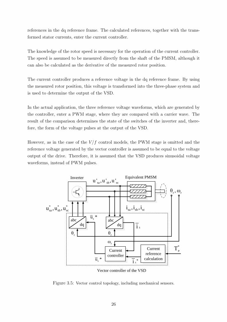
references in the dq reference frame. The calculated references, together with the trans-

formed stator currents, enter the current controller.

The knowledge of the rotor speed is necessary for the operation of the current controller.

The speed is assumed to be measured directly from the shaft of the PMSM, although it

can also be calculated as the derivative of the measured rotor position.

The current controller produces a reference voltage in the dq reference frame. By using

the measured rotor position, this voltage is transformed into the three-phase system and

is used to determine the output of the VSD.

In the actual application, the three reference voltage waveforms, which are generated by

the controller, enter a PWM stage, where they are compared with a carrier wave. The

result of the comparison determines the state of the switches of the inverter and, there-

fore, the form of the voltage pulses at the output of the VSD.

However, as in the case of the V/f control models, the PWM stage is omitted and the

reference voltage generated by the vector controller is assumed to be equal to the voltage

output of the drive. Therefore, it is assumed that the VSD produces sinusoidal voltage

waveforms, instead of PWM pulses.

Equivalent PMSM

r rθ , ω

Inverter

abcdq

* * *

sa sb scu ,u ,u

sa sb scu ' , u ' , u '

abcdq

sa sb sci , i , i

Current

controller

Current

reference

calculation

Si

S*isu *

rθ rθ

rω

su *

Vector controller of the VSD

*

eT

Figure 3.5: Vector control topology, including mechanical sensors.

26

3.5.2 Need for constant torque reference

The PMSM in the studied application needs to operate under constant-torque control.

The multiphase pump accommodates fluid stream of varying composition. This stream

consists of oil, gas and water, the analogy of which changes with time. Due to the varying

mass density of the stream mixture, the load of the PMSM also changes with time.

By applying a constant torque reference in the vector controller, the speed of the motor-

pump assembly can be regulated rapidly in response to load variations. This behaviour

corresponds to the desired operation of the system.

3.5.3 Current reference calculation

As was discussed in Section 3.1.1, the only torque-producing current component in

PMSMs with surface-mounted magnets is the q-axis current. The reference i∗sq for this

component can be calculated from (3.7) as

i∗sq =2

3npΨm

T ∗e (3.29)

where T ∗e is the electromagnetic torque reference. Regarding the reference i∗sd of the d-axis

stator current, it is usually selected in such a way, that the efficiency of the PMSM is

maximized. In general, its optimal value can be obtained by the MTPA method [34, 36]

according to

i∗sd =Ψm −

√Ψ2m + 8(Lsq − Lsd)2(i∗s)2

4(Lsq − Lsd)(3.30)

where i∗s is the reference of the stator current amplitude. In PMSMs with surface-mounted

magnets, the d-axis current does not contribute to any torque production and the maxi-

mum torque-to-current ratio is obtained by simply setting i∗sd = 0 [30, 39].

Since no dq saliency is considered for the PMSM in this thesis, the d-axis current reference

is set to zero for speeds lower than the rated speed ωr,rated. However, when operation

above ωr,rated is desired, the reference i∗sd needs to be modified by applying a proper field-

weakening strategy. Such a strategy is discussed in the section of the position-sensorless

vector controller.

27

3.5.4 Transfer function of the controlled system

Before the vector controller can be designed, the transfer function of the controlled sys-

tem must be derived. This system includes the PMSM and the transmission components,

namely the cable and the two transformers.

For PMSMs with surface-mounted magnets, the d-axis and q-axis inductances are ap-

proximately equal. Considering equivalent motor quantities, the flux-linkage equation

(3.2) can then be written as

ψ′s = L′sis + Ψm (3.31)

By substituting (3.31) into (3.1), the equivalent stator voltage u′s is given by

u′s = R′sis + L′sdisdt

+ jωrL′sis + jωrΨm (3.32)

where the term jωrΨm is the back-EMF e of the PMSM (according to (3.3)) and jωrL′sis

is the cross-coupling term.

The cross-coupling effect, thus the inherent interaction between the d-axis and q-axis

quantities of the PMSM, prevents the independent control of isd and isq, as can be demon-

strated through the d-axis and q-axis voltage equations of the motor.

According to (3.4), a variation in usd results in a desirable change in isd. However, due

to the d-axis component of the cross-coupling term in (3.5), the voltage usq is also forced

to change, which in turn causes an undesirable variation in isq. In effect, a change in isd

is inevitably accompanied by a change in isq and vice versa.

By applying the Laplace transform and rearranging terms, (3.32) becomes

is =1

sL′s +R′s + jωrL′s(u′s − e) (3.33)

Equation (3.33) represents the transfer function of the physical system that consists of

the PMSM and the transmission components.

3.5.5 Inclusion of compensating terms

In order to improve the performance of the current regulation, it is necessary to modify

the transfer function of the physical system (obtained from (3.33)) by including certain

28

compensating terms in the vector controller [35].

As was demonstrated in Section 3.5.4, the inherent cross-coupling in the PMSM prevents

the independent regulation of the d-axis and q-axis currents, thus the separate control of

the flux and the torque of the motor.

The negative impact of the cross-coupling effect on the performance of the controller can

be mitigated by compensating for the term jωrL′sis in (3.32). Clearly, the compensation

demands the knowledge of the stator current and the motor speed and its precision de-

pends on the accuracy of the estimation of the equivalent stator inductance L′s.

The control performance can be further improved by cancelling out the effect of the back-

EMF of the PMSM, thus by compensating for the term jωrΨm in (3.32). By feeding-

forward this term in the vector controller, the interaction between the electrical and the

mechanical dynamics of the motor is eliminated.

Finally, the term Rais can be added on the right-hand side of (3.32). The value Ra is

called active-damping resistance and is used to effectively increase the resistance R′s of the

system. Its presence in the controller increases the damping of the system and therefore

improves its response to disturbances. Of course, since Ra is a control parameter and not

a physical resistance, it does not contribute to any losses.

The block diagram of the physical system with the added compensating terms is shown

in Fig. 3.6.

s s r s

1

sL R j L

+_su

r me j

Si++

+

comp r me j

r sj L R

Physical system

Figure 3.6: Block diagram of the physical system with the added compensating terms.

After cancelling out the back-EMF and the cross-coupling term of the PMSM and after

29

introducing the active-damping resistance in the vector controller, (3.33) becomes

is =u′s

sL′s +R′s +Ra

(3.34)

Equation (3.34) represents the modified transfer function of the system, thus the transfer

function that is considered for the design of the controller.

3.5.6 Design of the PI regulator

The use of the dq reference frame, which results in the transformation of steady-state AC

quantities into DC values, makes it possible to use PI regulators for current control. The

reason is that integrators are well-suited for the control of DC quantities, because they

provide infinite gain at zero frequency and can therefore ensure the absence of steady-

state errors.

The relation between the input (i∗s − is) and the output u∗s of the PI current regulator is

given by

u∗s = (kp +kis

)(i∗s − is) (3.35)

where kp is the proportional gain, ki is the integral gain and i∗s is the space vector of the

stator current reference. The mission of the PI regulator is to provide current control

to the modified system, which was shown in Fig. 3.6. The current-controlled system is

presented in Fig. 3.7.

The PI regulator is designed according to the IMC method [35]. The closed-loop system,

which consists of the modified transfer function of the controlled system (given by (3.34)),

the transfer function of the PI regulator (given by (3.35)) and unit feedback, is designed

to be a first-order system with bandwidth ac. The gains of the PI regulator can then be

readily obtained as

kp = acL′s (3.36)

ki = ac(R′s +Ra) (3.37)

where the active-damping resistance Ra can be calculated from

Ra = acL′s −R′s (3.38)

30

+_++

+

Physical system

ip

kk

s

Modified system

+

_

PI regulator

comp r me j

r me j

s s r s

1

sL R j L

su *Si

Si

S*i

r sj L R

Figure 3.7: Block diagram of the current-controlled system, consisting of the physical system,the compensating terms and the PI regulator.

The bandwidth ac of the current regulator corresponds to a frequency which is selected

to be several times lower than the switching frequency of the VSD. The value of ac

determines the response speed of the controller according to

tr =ln9

ac(3.39)

where tr is the rise time, thus the time needed by the controlled currents to change from

10% to 90% of their final value.

3.5.7 Implementation of voltage and current limiters

The design of the vector controller must ensure that the electrical limits of the PMSM

and the VSD are not exceeded [31]. The value of the stator current reference must not

be greater than the rated current of the PMSM, while the the commanded voltage must

not exceed the maximum voltage capability of the VSD.

The limits of the current references i∗sd and i∗sq can be expessed as

i∗sd ≤ is,max (3.40)

i∗sq ≤√

(is,max)2 − (i∗sd)2 (3.41)

where is,max is the maximum acceptable stator current, which is equal to the peak value of

the rated current of the PMSM, thus is,max = is,rated. The limit of the voltage amplitude

reference u∗s can be written as

31

u∗s ≤ us,max (3.42)

where us,max is the maximum acceptable voltage at the output of the VSD.

The purpose of the implemented voltage and current limiters is to protect the PMSM

and the VSD. However, it should be noted that when the current or voltage limits are

hit, the intervention of the limiters causes the system to enter a practically uncontrolled

state, which includes distorted current responses and higher rise times.

One particular issue concerning the voltage limiter is integrator windup. When the volt-

age limit is hit, the current error (i∗s− is) becomes high, since the controller is not allowed

to provide the voltage that is required to achieve i∗s = is. Integrating this error would

result in a large ouput for the integrator, which should be decreased later, causing a

substantial current overshoot [26].

In order to prevent integrator windup, an anti-windup function is implemented in the

controller. Its idea is to cancel out the current error that results from the difference

between the unlimited voltage u∗s and the limited voltage u∗s,lim. The output of the anti-

windup function is given by

iaw =1

kp(u∗s,lim − u∗s) (3.43)

where iaw represents the error term due to the action of the voltage limiter. This term

is added to the current error (i∗s − is) which enters the integrator. The complete current-

controlled system, with the current limiters and the anti-windup function included, is

presented in Fig. 3.8.

3.6 Position-sensorless vector control

The operation of the vector control scheme which was described in Section 3.5 is based

on the presence of mechanical sensors.

This section explains why mechanical sensors need to be eliminated and describes differ-

ent position-estimating methods which can facilitate sensorless operation of the PMSM.

Based on one of these methods, a position-estimating algorithm has been implemented

and is presented.

In order to extend the speed range of the PMSM, the option of applying a field-weakening

32

+_++

+

Physical system

Modified system

PI regulator

+

_

Voltage limiterCurrent limiter

p

1

k

+

_

Anti-windup function

S*iS

*i S,limi *i

p

kk

s

su *

su *

s,limu *

comp r me j

r me j

s s r s

1

sL R j L

Si

r sj L R

Si

Figure 3.8: Block diagram of the current-controlled system, consisting of the modified system,the PI regulator, the current and voltage limiters and the anti-windup function.

strategy is investigated for the position-sensorless vector controller. After evaluating the

suitability of the studied system for the application of such a strategy, a field-weakening

algorithm is derived and is integrated into the vector controller.

Apart from the position estimator and the field-weakening algorithm, the other parts of

the controller are the same as the ones presented in Section 3.5.

3.6.1 Necessity of eliminating the position sensor

The presence of position sensors in PMSMs is usually undesirable, since it increases the

cost and the complexity of the system. When it comes to harsh subsea environments, it

is particularly important for the system to be as simple and robust as possible. The use

of position-sensorless control schemes is therefore a necessity.

The drawbacks of position sensors include an increased number of connections between

the motor and the control system, increased electromagnetic interference due to the pres-

ence of connecting leads and limited measuring accuracy due to environmental factors,

such as temperature, humidity and vibrations [25].

Moreover, the cost of the position-encoding device increases the overall cost of the system,

while the static and dynamic friction of the sensors are added on top of the mechanical

load of the motor [25, 27].

33

3.6.2 Review of position estimation methods

The operation of sensorless vector control schemes is facilitated by the development of

techniques that estimate the rotor position θr. Different methods have been proposed for

this purpose, some of which are shortly discussed in the section.

Back-EMF-based methods

By measuring the stator currents and voltages of the motor, the space vector of the back-

EMF in the αβ reference frame can be calculated. The obtained back-EMF vector can

then be used to determine the rotor position.

Back-EMF-based methods cannot be used at a standstill or during low-speed operation

of the PMSM, mainly because the back-EMF becomes too low in this range of speeds [27].

Furthermore, in order to calculate the back-EMF of the PMSM, the derivative of the

measured stator current is used, which makes these methods prone to noise [28].

The accuracy of the estimation is also affected by errors in the values of the motor

parameters [26].

Flux linkage-based methods

If the stator currents and voltages are known, the stator flux linkage in the αβ reference

frame can be calculated and used for the determination of the rotor position.

Due to the integration process by which the flux linkage is obtained, flux linkage-based

methods often suffer from the effects of integrator drift, which are compensated by analog

electronics or software techniques [28].

The accuracy of the position estimation is also affected by motor parameter variations

[25].

Inductance-based methods

Inductance-based techniques can be used to estimate the rotor position in PMSM topolo-

gies in which the stator inductances vary significantly over an electrical cycle [28].

The estimation in this case can be based on look-up tables, which contain information

about the relation between the stator inductances and the rotor position [26].

34

Problems with these methods may include the requirement of high switching frequency

for the accurate calculation of the inductances, as well as sensitivity to certain parameter

variations [26].

Observer-based methods

In observer-based techniques, a mathematical model of the system is created and is sup-

plied with the same excitation as the actual system. This model produces estimated

outputs, which are compared with the measured outputs of the real system. The errors

between the estimated and the measured quantities are used to correct the outputs of

the observer [27].

Since the PMSM model is nonlinear, the design of a state observer is generally quite

complex. The used algorithms may often be robust against parameter variations and

measurement noise, but they have high computational requirements [26].

Selection of estimation method

The estimation scheme which has been implemented in this thesis is flux linkage-based.

It uses a thoroughly tested algorithm, which provides accurate position estimation within

a wide speed range.

The issue of integrator drift, which is often considered to be the main drawback of flux

linkage-based methods, is resolved by constantly correcting and updating the estimated

quantities, by using the available current measurements.

Other methods could also provide adequate control performance for the studied applica-

tion. Back-EMF-based methods, for instance, have proved to be quite popular and would

probably be suitable for the studied system. Their inability to provide accurate position

estimation at low speeds would not be a problem, since low-speed operation is handled

by the V/f controller anyway.

Inductance-based methods however, would not be a sensible choice, since they are only

well-suited to motors with significant inductance variations over one electrical period. As

the considered motor has negligible dq saliency, the resulting variations would be too low

to produce a proper position estimation.

35


The structure of the designed position-sensorless vector controller is presented in Fig. 3.9.

In contrast to the layout presented in Fig. 3.5, no mechanical sensors are present in the

new topology. Although this increases the robustness of the system, it also complicates

the design of the vector controller.

The elimination of the mechanical sensors has been achieved by adding a position esti-

mator in the controller. The mission of the estimator is to provide position estimates

to the dq transformation blocks and speed estimates to the current controller. The in-

puts required by the estimator are two phase currents and a previously generated voltage

reference.

Equivalent PMSMInverter

abcdq

* * *

sa sb scu ,u ,u

sa sb scu ' , u ' , u '

abcdq

sa sb sci , i , i

Current

controller

Current

reference

calculation

Si

S*isu *

rθ rθ

rω

su *

Vector controller of the VSD

*

eT

Position

estimator

rθ rω

su *

Figure 3.9: Position-sensorless vector control topology.

3.6.4 Implementation of the position estimator

The implemented estimator estimates the rotor position θr, by executing a multi-step

discretized algorithm. Its operation is based on a method described in [26], although

variations of this method have been earlier presented in [25, 28, 29].

For the design of the position estimator, it is convenient to use the αβ reference frame. In

36

contrast to the dq frame, which is synchronized to the rotation of the PMSM rotor, the αβ

frame is stationary and its α axis is aligned with the a axis of the three-phase system [35].

Figure 3.10 provides an overview of the functions executed by the position estimator.

The steps of the discretized estimating algorithm are discussed in more detail below.

Flux linkage

estimation

s

su 1

s

si

s

s,est Current

estimation

r,pr

s

s,esti Position

correction

r,pr r,cor Position

prediction r,pr 1

s

s,upd 1 r,est Speed

estimation

Position

compensation

r,est Flux linkage

updating

s

si

r,cor

s

s,upd

Figure 3.10: Block diagram of the position estimator.

Flux linkage estimation

The first step of the algorithm is the estimation of the equivalent stator flux linkage. By

considering equivalent motor quantities, (3.1) can be represented in the αβ frame as

u′ss = Rsi

ss +

dψ′ss

dt(3.44)

The representation of the αβ vectors is similar to the one of the dq vectors. The only

difference is the additional superscript ’s’, which denotes that αβ vectors are stationary.

By using discretized quantities and integrating, (3.44) can be written as

ψ′ss,est(κ) = Ts[u′

ss(κ− 1)−R′siss(κ)] + ψ′

ss,upd(κ− 1) (3.45)

where Ts is the sampling period, κ is the sampling number and the subscripts ’est’ and

’upd’ denote estimated and updated values respectively. For the discrete integration of

the difference between the stator voltage and the resistive drop, the rectangular rule has

been applied.

Equation (3.45) estimates the equivalent stator flux linkage, based on the generated volt-

age reference and the updated flux linkage of the previous sampling period κ− 1, as well

as on the stator current, which is measured in the current period κ.

The flux linkage and stator voltage values of the previous sampling period are obtained

37

by including unit delay blocks in the controller. By storing signals for a specified amount

of sampling periods, these blocks allow the controller to access previous values of its

variables.

Current estimation

The second step of the algorithm is the estimation of the stator current, based on the

estimated flux linkage ψ′ss,est. Equation (3.31) can be represented in the αβ frame as

ψ′ss = L′si

ss + Ψme

jθr (3.46)

The stator current can be estimated from

iss,est(κ) =ψ′ss,est(κ)−Ψme

jθr,pr(κ)

L′s(3.47)

where the subscript ’pr’ denotes predicted quantities. Equation (3.47) estimates the

stator currents by using the flux linkage obtained from the previous step and the position

predicted for the current sampling period.

Position correction and speed estimation

The third step of the algorithm is the correction of the previously predicted rotor posi-

tion. The current error, thus the difference ∆iss between the measured and the estimated

currents, is calculated and is transformed into the dq reference frame by using the pre-

dicted rotor angle θr,pr.

The presence of a current error indicates the need for position correction. It can be

proven, as in [26], that only the q-axis component ∆iq of the dq-transformed current

error ∆is is needed for the calculation of the position correction term ∆θr according to

∆θr(κ) = −L′s∆iq(κ)

Ψm

(3.48)

The corrected position is then obtained from the predicted position θr,pr and the correction

term ∆θr according to

θr,cor(κ) = θr,pr(κ) + ∆θr(κ) (3.49)

where the subscript ’cor’ denotes corrected values. The estimated speed ωr,est of the

PMSM is easily obtained from the discrete derivative of the corrected position according

to

38

ωr,est(κ) =θr,cor(κ)− θr,cor(κ− 1)

Ts(3.50)

The estimated speed passes through a low-pass filter, which eliminates the high-frequency

ripple that might be present, and is then directed to the current regulator of the vector

controller.

Flux linkage updating

The next step is to update the previously estimated flux linkage, so that the updated

value ψ′ss,upd can be used for the flux linkage estimation in the next sampling period.

Equation (3.46) was used earlier to estimate the stator currents from the estimated flux

linkage and the predicted position. By applying the same equation, this time using the

measured currents and the corrected position, the updated flux linkage can be obtained

as

ψ′ss,upd(κ) = L′si

ss(κ) + Ψme

jθr,cor(κ) (3.51)

By using the updated flux linkage ψ′ss,upd in the next sampling period, the negative effects

of integrator drift are avoided.

Position prediction

The next step of the algorithm is the prediction of the rotor position for the next sampling

period. A common assumption is that the position varies with time as a second-order

polynomial [25, 28]. The predicted position θr,pr can be calculated from

θr,pr(κ+ 1) = 3θr,cor(κ)− 3θr,cor(κ− 1) + θr,cor(κ− 2) (3.52)

where the previously estimated positions θr,cor(κ − 1) and θr,cor(κ − 2) are obtained by

using a single-period unit delay and a double-period unit delay respectively.

Position compensation

Tests on the implemented model revealed the presence of steady-state differences between

the estimated currents and the real currents of the system. Furthermore, it was noticed

that the magnitude of the estimation errors increased as the steady-state speed of the

PMSM increased.

In order to eliminate these estimation errors, a speed-dependent position compensator

39

has been included in the estimator. Its mission is to generate a compensating term θr,comp,

which increases linearly with the estimated motor speed ωr,est and which is added to the

corrected position θr,cor.

In order to determine the linear function θr,comp = f(ωr,est) of the compensating block, the

required compensation θr,comp for two different speeds is obtained by trial and error. The

straight line which passes from the two position-speed pairs corresponds to the transfer

function of the position compensator.

3.6.5 Basic idea of field-weakening

A field-weakening strategy has been applied in the sensorless vector controller, in order

to extend the operating speed range of the PMSM. Before the implemented algorithm is

presented, the fundamental principles of field-weakening are briefly discussed.

Assuming that the stator flux linkage of the PMSM is constant and that the resistive

stator voltage drop is negligible, the stator voltage equation is given by (3.14). By

solving for the electrical speed ωr, this equation yields

ωr 'us

ψs(3.53)

Equation (3.53) demonstrates that the speed of the motor can be increased either by

increasing the supplied voltage amplitude, or by decreasing the stator flux linkage.

When the PMSM operates below its rated speed, the flux linkage should be kept around

its nominal value, so that optimal efficiency is achieved, according to the discussion in

Section 3.3.1. The speed in this case can be adjusted by varying the supplied voltage

amplitude.

Speed control through the voltage amplitude is possible up to the rated speed of the mo-

tor. In order to increase the speed even further, without exceeding the rated voltage of

the PMSM, it is necessary to decrease the amplitude of the stator flux linkage. Therefore,

for high-speed operation of the motor, field-weakening is needed.

According to (3.2), a reduction of the flux linkage amplitude can be achieved by injecting

a negative d-axis current into the motor. Since the d-axis current does not contribute to

any torque production, field-weakening results in a decreased torque-to-current ratio.

Moreover, since the overall stator current cannot exceed its rated value, an increase of

40

the d-axis current restricts the maximum acceptable q-axis current and therefore the

maximum torque that the PMSM can produce.

Based on the previous discussion, two control regions can be identified for the PMSM.

The ’voltage control’ region corresponds to constant maximum torque and power which

increases with speed, while the ’flux control’ region corresponds to constant power and

maximum torque which decreases with speed [32, 40].

3.6.6 Overvoltage risk during field-weakening

When it comes to field-weakening, an issue that needs special attention is the risk of

exceeding the voltage withstand limits of the VSD [36].

According to (3.3), the magnitude of the back-EMF is proportional to the speed of the

motor. Therefore, the high speeds which are reached during the field-weakening opera-

tion result in high back-EMF values.

If the stator current is suddenly lost for some reason, the voltage drop in the transmission

system and the stator impedance becomes zero and the inverter of the VSD experiences

a voltage equal to the back-EMF of the PMSM.

In order to avoid damaging the inverter, it is necessary to design the VSD so that it can

withstand the maximum back-EMF that can be reached during field-weakening [33].

For a VSD with a specified voltage output capability, it is necessary to limit the maximum

speed during the field-weakening operation, so that the resulting back-EMF does not

exceed the maximum voltage of the inverter [34].

3.6.7 Field-weakening capability of the system

Some systems provide favourable conditions for field-weakening operation, while others

do not. This section evaluates the possibility of applying a field-weakening strategy in

the studied system. The evaluation is based on considerations on the mechanical load

and the system inductances.

In order to increase the motor speed above its rated value, a negative d-axis current is

required, as was discussed in Section 3.6.5. Since the speed increase cannot be achieved

without a torque increase for the considered load, the q-axis current needs to be increased

as well.

41

Therefore, a speed increase with field-weakening requires a rise in the magnitude of both

d-axis and q-axis currents and, as a result, an increase of the overall current magnitude.

Therefore, the degree to which the speed range of the PMSM can be extended by means

of field-weakening depends on how soon the current limit of the motor is reached after

exceeding the rated speed.

The available current margin depends on how high the load torque is. In the case of a

light load, the stator current at rated speed is low and the current margin is high.

As explained in Section 3.6.5, the maximum torque that can be produced in the field-

weakening region decreases as the speed increases. On the other hand, the actual pro-

duced torque increases with speed, due to the considered load characteristic.

The point at which the maximum and the actual torque become equal defines the maxi-

mum speed that can be reached with field-weakening. This is also the point at which the

stator current reaches its rated value.

The field-weakening capability of the system is heavily dependent on the d-axis induc-

tance of the PMSM. It can be observed from (3.2) that for low values of this inductance,

the contribution of the d-axis current on the stator flux linkage decreases, which results

in limited field-weakening capability.

In general, PMSMs with small dq saliency, such as the motor considered in this thesis,

are characterized by low inductances, which makes them unsuitable for field-weakening

operation [36].

Of course, it should be borne in mind that the controlled system does not include only the

motor, but the transmission system as well. Therefore, the inductance of the equivalent

motor includes the inductances of the cable and the transformers and, therefore, it is

significantly higher than the inductance of the actual motor.

Although the transmission components may appear to have a positive effect on the field-

weakening capability of the system, this effect is counterbalanced by the higher voltage

that the VSD needs to provide, in order to compensate for the voltage drop in the trans-

mission system.

42

During field-weakening operation, the voltage drop in the transmission components rises,

due to the increased current magnitude. This means, that in order to supply the motor

with its rated voltage, the VSD must increase its voltage output.

3.6.8 Derivation of the field-weakening algorithm

The implemented field-weakening algorithm is based on an open-loop method presented

in [34]. Its mission is to generate a proper d-axis current reference, when the desired

speed is higher than the rated speed of the PMSM.

For the derivation of the field-weakening function, it is assumed that the motor operates

at steady state and that the resistive stator voltage drop is negligible. The latter assump-

tion is stronger for motors with high voltage and low current ratings [30].

Under the aforementioned assumptions, the d-axis and q-axis stator voltages (given by

(3.4) and (3.5) respectively) can be written as

usd = −ωrLsisq (3.54)

usq = ωrLsisd + ωrΨm (3.55)

The stator voltage amplitude us must not exceed the rated voltage us,rated, thus

us ≤ us,rated ⇒√

(usd)2 + (usq)2 ≤ us,rated (3.56)

In the implemented field-weakening algorithm, the voltage us,rated is calculated from (3.54)

- (3.56), by considering the rated speed ωr,rated of the PMSM.

During field-weakening operation, the voltage amplitude us is equal to us,rated. By sub-

stituting (3.54) and (3.55) into (3.56) and by solving for the d-axis current isd, the d-axis

current reference i∗sd is obtained as

i∗sd = −Ψm

Ls+

1

Ls

√(us,ratedωr

)2 − (Lsisq)2 (3.57)

Equation (3.57) is used for the calculation of the d-axis current reference when the es-

timated speed exceeds the rated speed ωr,rated of the PMSM. For operation below this

speed, i∗sd is set to zero, according to the discussion in Section 3.5.3.

43

For the calculation of the d-axis current reference from (3.57), the field-weakening block

uses the speed ωr,est produced by the position estimator (according to (3.50)) and the

q-axis current reference i∗sq calculated from (3.29) during the previous sampling period.

The magnitude of the calculated d-axis current reference is limited by the current limiter

(as discussed in Section 3.5.7) and is then supplied to the PI regulator of the current

controller.

44

Chapter 4

Simulation results

This chapter presents the obtained simulation results for the designed control models.

Several startup tests are performed, in order to investigate the performance of the im-

plemented V/f controllers and in order to optimize their parameters. Their ability to

accelerate the PMSM for different initial rotor positions and their effectiveness in dealing

with sudden load variations are verified.

Furthermore, the behaviour of the system during the transition from V/f control to vec-

tor control is investigated and the response of the designed vector controllers to load steps

is tested.

The vector control scheme with the mechanical sensors is subjected to a startup test,

so that the performance of the current regulator is verified, while the behaviour of the

position estimator and the effectiveness of the implemented field-weakening alogrithm of

the position-sensorless controller are evaluated through different simulations.


This section presents the simulation results for the implemented open-loop V/f controller.

In order to determine the settings that optimize the performance of the controller, sim-

ulations with different parameter values are performed. When it comes to V/f control

schemes, it is common to select the settings of the controller by trial and error [21].

In order to ensure that the PMSM startup is successful for every initial rotor position,

the behaviour of the system is investigated for several starting angles.

45

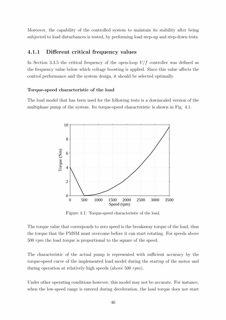
Moreover, the capability of the controlled system to maintain its stability after being

subjected to load disturbances is tested, by performing load step-up and step-down tests.

4.1.1 Different critical frequency values

In Section 3.3.5 the critical frequency of the open-loop V/f controller was defined as

the frequency value below which voltage boosting is applied. Since this value affects the

control performance and the system design, it should be selected optimally.

Torque-speed characteristic of the load

The load model that has been used for the following tests is a downscaled version of the

multiphase pump of the system. Its torque-speed characteristic is shown in Fig. 4.1.

0 500 1000 1500 2000 2500 3000 35000

2

4

6

8

10

Speed (rpm)

Tor

que

(Nm

)

Figure 4.1: Torque-speed characteristic of the load.

The torque value that corresponds to zero speed is the breakaway torque of the load, thus

the torque that the PMSM must overcome before it can start rotating. For speeds above

500 rpm the load torque is proportional to the square of the speed.

The characteristic of the actual pump is represented with sufficient accuracy by the

torque-speed curve of the implemented load model during the startup of the motor and

during operation at relatively high speeds (above 500 rpm).

Under other operating conditions however, this model may not be accurate. For instance,

when the low-speed range is entered during deceleration, the load torque does not start

46

increasing, as indicated by the characteristic in Fig. 4.1.

In other words, the low-speed part of the presented load curve represents the difficulty of

the system to overcome the static friction of the pump during the startup, but it cannot

represent the low-speed behaviour of the pump under all operating conditions.

Effect of the critical frequency on the applied V/f ratio

The boosting factor Fb as a function of the critical frequency fcr has been obtained from

(3.15) and is plotted in Fig. 4.2. The equivalent stator resistance R′s in (3.15) has been

calculated by assuming that the length of the cable is such, that the voltage drop in the

transmission system is approximately 10%. This requirement yields a length of around

10 km.

2 4 6 8 102

4

6

8

10

12

14

Critical frequency (Hz)

Boo

stin

g fa

ctor

Figure 4.2: Boosting factor Fb as a function of the critical frequency fcr.

Figure 4.2 demonstrates that the boosting factor increases significantly, as the critical

frequency decreases. Since the applied V/f ratio is proportional to the boosting factor

Fb, according to (3.16), this ratio increases for low critical frequency values.

As was discussed in Section 3.2.2, high V/f ratios result in the necessity of oversizing

the topside transformer of the system. In order to minimize the size and cost of this

transformer, it is necessary to minimize the applied V/f ratio, by selecting the maximum

acceptable critical frequency.

47

The aim of the following tests is to determine the maximum critical frequency for which

the PMSM can start safely.

Applied frequency reference curve

The slope of the frequency reference in the following tests is selected to be 0.83 Hz/s.

Fig. 4.3 shows the applied frequency reference curve.

0 1 2 3 4 5 60

1

2

3

4

5

Time (s)

Freq

uenc

y (H

z)

Figure 4.3: Applied frequency reference f∗.

A separate investigation on the effect of the frequency slope on the control performance

is conducted in Section 4.1.2.

Startup test with low critical frequency

Initially, the behaviour of the open-loop V/f controller is investigated for fcr = 3 Hz.

The startup performance of the PMSM in this case is shown in Fig. 4.4.

Figure 4.4 a) presents the waveform of the voltage amplitude reference u∗s. Voltage

boosting is applied until 3.6s, thus until the time instant that corresponds to the selected

critical frequency of 3 Hz.

Since the applied frequency increases at a steady rate, the V/f ratio takes its maximum

value during the voltage-boosting interval. This value determines the size of the topside

transformer of the system.

48

0 2 4 60

50

100

Time (s)

Vol

tage

(V

)

a)

0 2 4 6−500

0

500

Time (s)

Spe

ed(r

pm)

b)

nr

nr,ref

0 2 4 60

5

10

Time (s)

Ang

le (

rad)

c)

θ

r

θr,ref

0 2 4 6−10

0

10

Time (s)

Tor

que

(Nm

)d)

Figure 4.4: Waveforms for fcr = 3 Hz. a) Voltage amplitude reference u∗s. b) Actual speednr and speed reference n∗r . c) Actual position θr and position reference θ∗r . d) Electromagnetictorque Te.

It can be found by combining Fig. 4.3 and 4.4 a) (or by using (3.16)) that the V/f ratio

that is applied during the initial accelerating interval is approximately equal to 24.17

V/Hz. Compared to the rated ratio of the PMSM (4.90 V/Hz), this value is extremely

large and increases the required size of the topside transformer significantly.

Figure 4.4 b) presents the waveforms of the mechanical rotor speed nr and the speed

reference n∗r. It is apparent that the startup in this case is successful, since the motor

manages to establish synchronism with the supplied field after a few oscillations.

It is worth noticing that the PMSM rotates in the negative direction for a short time

interval, before starting to accelerate in the positive direction. The maximum negative

speed that is reached in this interval is around 26.5 rpm. The issue of temporary reverse

rotation is common for PMSMs [22, 23, 29] and is investigated further in Section 4.1.3.

Figure 4.4 c) shows the waveforms of the rotor position θr and the position reference θ∗r .

Due to the inertia of the rotor and the load, it takes some time (approximately 2s) for

the PMSM to follow the rotation of the supplied field.

In Fig. 4.4 d), the waveform of the electromagnetic torque Te is presented. The initial lack

of synchronism is accompanied by torque oscillations. For a while, the torque becomes

negative, reaching a negative maximum of 4.6 Nm, which causes the reverse rotation of

Fig. 4.4 b).

49

Figure 4.5 shows the voltages and currents at the output of the VSD.

0 2 4 6−100

0

100

Time (s)

Vol

tage

(V

)

a)

0 2 4 6−20

0

20

Time (s)

Cur

rent

(A

)

b)

0 2 4 6−100

0

100

Time (s)

Vol

tage

(V

)

c)

u‘sd

u‘sq

0 2 4 6−20

0

20

Time (s)

Cur

rent

(A

)

d)

isd

isq

Figure 4.5: Waveforms for fcr = 3 Hz. a) Equivalent stator voltages u′sa, u′sb, u

′sc. b) Stator

currents isa, isb, isc. c) Equivalent stator voltages u′sd, u′sq. d) Stator currents isd, isq.

The gradual increase of the electrical frequency and voltage magnitude is demonstrated

in Fig. 4.5 a), while Fig. 4.5 b) shows that the stator current amplitude is high during the

startup (reaching an rms value of over 9.9 A), temporarily exceeding the rated current

of the PMSM.

High startup currents are a common problem in open-loop V/f control schemes. For

instance, such a scheme was tested in [21] and its starting performance was evaluated as

poor, due to the initial overcurrents experienced by the PMSM.

Figure 4.5 d) reveals that the high stator current can be mainly attributed to the high

magnetizing current isd, which indicates that the PMSM experiences overexcitation dur-

ing its startup. A similar case was presented in [20]. Since V/f control does not allow

direct current control, it cannot provide optimal efficiency during the startup process.

The torque-producing current component isq on the other hand, is rather low. It reaches

a maximum value quite early, but then gradually falls, after the breakaway torque of the

system is overcome.

Figure 4.6 presents the voltages of the PMSM.

50

0 2 4 6−50

0

50

Time (s)

Vol

tage

(V

)

a)

0 2 4 6−20

0

20

40

Time (s)

Vol

tage

(V

)

b)

usd

usq

Figure 4.6: Waveforms for fcr = 3 Hz. a) Stator voltages usa, usb, usc. b) Stator voltages usd,usq.

It can be observed by comparing Fig. 4.5 and Fig. 4.6 that the presence of the transmis-

sion system causes a temporary distortion in the waveforms of the motor voltage. More

importantly, the voltage drop in the transmission components reduces the PMSM voltage

significantly.

Although the cable length in the performed tests has been selected such, that the steady-

state voltage drop is approximately 10% of the VSD voltage, this drop becomes almost

70% at 4s. The reason for this extremely high value is the high startup current, which

was observed in Fig. 4.5.

Startup test with medium critical frequency

For the next test, the critical frequency is increased to fcr = 6 Hz. The startup behaviour

of the PMSM in this case is shown in Fig. 4.7.

It can be found from Fig. 4.3 and 4.7 a) that the V/f ratio that is applied during the

voltage-boosting interval is approximately equal to 14.44 V/Hz. Although this value is

higher than the rated V/f ratio of the PMSM, it is approximately 40% lower than in the

case of fcr = 3 Hz.

However, it is obvious from Fig. 4.7 that the decreased V/f ratio during the voltage-

boosting interval comes at the cost of worse control performance. The reduced voltage

that is provided to the PMSM during the early accelerating stage makes it harder for the

rotor to establish synchronism with the supplied field.

As shown in Fig. 4.7 d), the torque oscillations are more severe in this case, reaching

a higher negative maximum of approximately 6.1 Nm. These oscillations result in two

intervals of negative speed, as shown in Fig. 4.7 b). In this case, the PMSM reaches a

maximum negative speed of around 63.2 rpm.

51

0 2 4 6 80

50

100

Time (s)

Vol

tage

(V

)

a)

0 2 4 6 8−500

0

500

Time (s)

Spe

ed(r

pm)

b)

nr

nr,ref

0 2 4 6 80

5

10

Time (s)

Ang

le (

rad)

c)

θ

r

θr,ref

0 2 4 6 8−10

0

10

Time (s)

Tor

que

(Nm

)d)


Figure 4.7 c) demonstrates that it takes around 2.8s for the rotor to establish synchro-

nism with the field, which is 40% more than in the case of fcr = 3 Hz.

Figure 4.8 presents the voltages and currents at the output of the VSD.

0 2 4 6 8−100

0

100

Time (s)

Vol

tage

(V

)

a)

0 2 4 6 8−20

0

20

Time (s)

Cur

rent

(A

)

b)

0 2 4 6 8−100

0

100

Time (s)

Vol

tage

(V

)

c)

u‘sd

u‘sq

0 2 4 6 8−20

0

20

Time (s)

Cur

rent

(A

)

d)

isd

isq


′sc. b) Stator


It can be found from Fig. 4.8 b) that the stator current is even higher than in the case

52

of fcr = 3 Hz (reaching an rms value of over 10.4 A). Compared to 4.5 b), the current

waveform in this case is more distorted, as a result of the increased difficulty of the PMSM

to achieve synchronism.

The voltages of the PMSM are presented in Fig. 4.9.

0 2 4 6 8−50

0

50

Time (s)

Vol

tage

(V

)

a)

0 2 4 6 8−20

0

20

40

Time (s)

Vol

tage

(V

)

b)

usd

usq

Figure 4.9: Waveforms for fcr = 6 Hz. a) Stator voltages usa, usb, usc. b) Stator voltages usd,usq.

Similarly to the case of fcr = 3 Hz, the distortion in the voltage waveforms of the motor

is noticeable and the voltage drop in the transmission system becomes almost 60% at

7.5s.

Startup test with high critical frequency

For the next test, the critical frequency is increased to fcr = 9 Hz. The startup behaviour

of the PMSM in this case is shown in Fig. 4.10.

The applied V/f ratio has decreased to approximately 11.20 V/Hz, but the PMSM

startup is unsuccessful. As shown in Fig. 4.10 d), the motor experiences torque oscilla-

tions of increasing magnitude, which cause the rotor to vibrate, as can be seen in Fig. 4.10

b). The inability of the PMSM to establish synchronism is clearly demonstrated in 4.10 c).


The abnormal operation of the PMSM is reflected in the oscillations in the d-axis and

q-axis voltage and current waveforms (shown in 4.11 c) and 4.11 d) respectively).

Selection of critical frequency

The performed tests clearly demonstrate that as the critical frequency of the V/f con-

troller increases, the V/f ratio of the VSD decreases, but the control performance dete-

riorates.

53

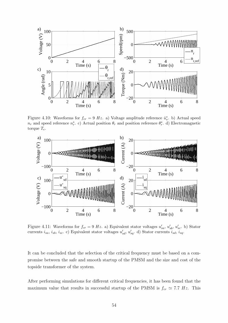
0 2 4 6 80

50

100

Time (s)

Vol

tage

(V

)

a)

0 2 4 6 8−500

0

500

Time (s)

Spe

ed(r

pm)

b)

nr

nr,ref

0 2 4 6 80

5

10

Time (s)

Ang

le (

rad)

c)

θ

r

θr,ref

0 2 4 6 8−20

0

20

Time (s)

Tor

que

(Nm

)d)


0 2 4 6 8−100

0

100

Time (s)

Vol

tage

(V

)

a)

0 2 4 6 8−20

0

20

Time (s)

Cur

rent

(A

)

b)

0 2 4 6 8−100

0

100

Time (s)

Vol

tage

(V

)

c)

u‘

sd

u‘sq

0 2 4 6 8−20

0

20

Time (s)

Cur

rent

(A

)

d)

isd

isq


′sc. b) Stator


It can be concluded that the selection of the critical frequency must be based on a com-

promise between the safe and smooth startup of the PMSM and the size and cost of the

topside transformer of the system.

After performing simulations for different critical frequencies, it has been found that the

maximum value that results in successful startup of the PMSM is fcr ' 7.7 Hz. This

54

value corresponds to a V/f ratio of about 12.30 V/Hz.

Since V/f control schemes are often prone to instability, due to their sensitivity to dis-

turbances (such as sudden load changes), a safety margin should be considered during

the selection of the critical frequency. Therefore, a value of fcr = 5.5 Hz, corresponding

to a V/f ratio of about 15.33 V/Hz, can be selected.

4.1.2 Different frequency reference slopes

For the tests in Section 4.1.1, the frequency reference slope was kept constant and equal to

0.83 Hz/s. In the following tests on the other hand, the critical frequency is kept constant

and equal to 5.5 Hz and the effect of the frequency slope on the control performance is

investigated.

Startup test with low frequency reference slope

Initially, the behaviour of the open-loop V/f controller is investigated for a frequency

slope of 0.5 Hz/s. The startup performance of the PMSM in this case is shown in Fig.

4.12.

0 2 4 6 80

2

4

Time (s)

Fre

quen

cy (

Hz)

a)

0 2 4 6 80

50

100

Time (s)

Vol

tage

(V

)

b)

0 2 4 6 8−500

0

500

Time (s)

Spe

ed(r

pm)

c)

nr

nr,ref

0 2 4 6 8−10

0

10

Time (s)

Tor

que

(Nm

)d)

Figure 4.12: Waveforms for df∗/dt = 0.5 Hz/s. a) Frequency reference f∗ b) Voltage amplitudereference u∗s. c) Actual speed nr and speed reference n∗r . d) Electromagnetic torque Te.

It can be seen in Fig. 4.12 d) that the motor experiences torque oscillations that last for

around 6s. The maximum negative value of these oscillations is approximately 6.1 Nm.

55

As a result, there are two intervals of negative speed, before synchronism is established.

It can be observed in Fig. 4.12 c) that the PMSM reaches a maximum negative speed of

approximately 64 rpm.


0 2 4 6 8−100

0

100

Time (s)

Vol

tage

(V

)

a)

0 2 4 6 8−20

0

20

Time (s)

Cur

rent

(A

)

b)

0 2 4 6 8−100

0

100

Time (s)

Vol

tage

(V

)

c)

u‘sd

u‘sq

0 2 4 6 8−20

0

20

Time (s)

Cur

rent

(A

)

d)

isd

isq

Figure 4.13: Waveforms for df∗/dt = 0.5 Hz/s. a) Equivalent stator voltages u′sa, u′sb, u

′sc. b)

Stator currents isa, isb, isc. c) Equivalent stator voltages u′sd, u′sq. d) Stator currents isd, isq.

The long duration of the oscillations in Fig. 4.13 c) and Fig. 4.13 d) reflects the difficulty

of the PMSM to establish synchronism. Moreover, the positive d-axis current in Fig. 4.13

d) indicates that the motor experiences overexcitation during its startup.

The current magnitude during the startup process exceeds the rated current of the PMSM

(reaching a maximum rms value of approximately 10.2 A at around 11.1s).


From Fig. 4.13 a) and Fig. 4.14 a), it can be found that the voltage drop in the

transmission system at 5.9s is approximately 61% of the VSD voltage.

Startup test with medium frequency reference slope

For the next test, the frequency slope is increased to 8 Hz/s. The startup behaviour of

the PMSM in this case is shown in Fig. 4.15.

56

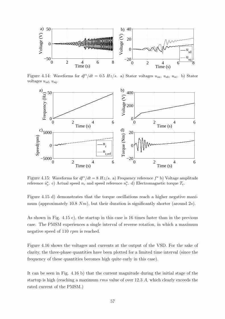
0 2 4 6 8−50

0

50

Time (s)

Vol

tage

(V

)

a)

0 2 4 6 8−20

0

20

40

Time (s)

Vol

tage

(V

)

b)

usd

usq

Figure 4.14: Waveforms for df∗/dt = 0.5 Hz/s. a) Stator voltages usa, usb, usc. b) Statorvoltages usd, usq.

0 2 4 60

50

Time (s)

Fre

quen

cy (

Hz)

a)

0 2 4 60

200

400

Time (s)V

olta

ge (

V)

b)

0 2 4 6−5000

0

5000

Time (s)

Spe

ed(r

pm)

c)

nr

nr,ref

0 2 4 6−20

0

20

Time (s)

Tor

que

(Nm

)d)

Figure 4.15: Waveforms for df∗/dt = 8 Hz/s. a) Frequency reference f∗ b) Voltage amplitudereference u∗s. c) Actual speed nr and speed reference n∗r . d) Electromagnetic torque Te.

Figure 4.15 d) demonstrates that the torque oscillations reach a higher negative maxi-

mum (approximately 10.8 Nm), but their duration is significantly shorter (around 2s).

As shown in Fig. 4.15 c), the startup in this case is 16 times faster than in the previous

case. The PMSM experiences a single interval of reverse rotation, in which a maximum

negative speed of 110 rpm is reached.

Figure 4.16 shows the voltages and currents at the output of the VSD. For the sake of

clarity, the three-phase quantities have been plotted for a limited time interval (since the

frequency of these quantities becomes high quite early in this case).

It can be seen in Fig. 4.16 b) that the current magnitude during the initial stage of the

startup is high (reaching a maximum rms value of over 12.3 A, which clearly exceeds the

rated current of the PMSM.)

57

0 0.5 1 1.5 2−200

0

200

Time (s)

Vol

tage

(V

)

a)

0 0.5 1 1.5 2−20

0

20

Time (s)

Cur

rent

(A

)

b)

0 2 4 6−500

0

500

Time (s)

Vol

tage

(V

)

c)

u‘sd

u‘sq 0 2 4 6

−20

0

20

Time (s)

Cur

rent

(A

)

d)

isd

isq

Figure 4.16: Waveforms for df∗/dt = 8 Hz/s. a) Equivalent stator voltages u′sa, u′sb, u

′sc. b)


Figure 4.16 d) shows that despite the initial overexcitation, the d-axis current becomes

negative after approximately 4.9s. As explained below, this result is related to the cross-

coupling effect in the PMSM.

As the load torque increases with speed, the q-axis current rises. This causes an increase

in the q-axis voltage according to (3.5) and a decrease in the d-axis voltage according to

(3.4). These considerations are in agreement with the results in Fig. 4.16 c).

The decrease in the d-axis voltage results in a decrease in the d-axis current according to

(3.4). Eventually, this current becomes negative, causing the PMSM to become under-

excited.


From Fig. 4.16 a) and Fig. 4.17 a) it can be found that the voltage drop in the trans-

mission system at the instant when the current magnitude is maximum (around 0.9s) is

approximately 60% of the VSD voltage.

Startup test with high frequency reference slope



58

0 0.5 1 1.5 2−100

0

100

Time (s)

Vol

tage

(V

)

a)

0 2 4 6−200

0

200

400

Time (s)

Vol

tage

(V

)

b)

usd

usq

Figure 4.17: Waveforms for df∗/dt = 8 Hz/s. a) Stator voltages usa, usb, usc. b) Statorvoltages usd, usq.

0 0.5 1 1.5 20

20

40

Time (s)

Fre

quen

cy (

Hz)

a)

0 0.5 1 1.5 20

100

200

Time (s)

Vol

tage

(V

)

b)

0 0.5 1 1.5 2−5000

0

5000

Time (s)

Spe

ed(r

pm)

c)

n

r

nr,ref

0 0.5 1 1.5 2−50

0

50

Time (s)

Tor

que

(Nm

)d)


Apparently, the startup in this case is unsuccessful. As shown in Fig. 4.18 d), the mo-

tor experiences torque oscillations of increasing magnitude, which result in mechanical

vibrations, as can be seen in Fig. 4.18 c).

As was discussed in Section 3.3.2, the rate at which the supplied frequency increases

should be kept adequately low. High values of the frequency slope (such as the one

selected in this test) may result in the inability of the rotor to follow the supplied field.

Selection of frequency reference slope

The performed tests demonstrate that for lower values of the frequency slope, it takes

more time for the PMSM to establish synchronism with the supplied field and to reach

its target speed.

59

Higher slopes on the other hand, result in faster accelerations and make it possible for

the PMSM to get synchronized with the field earlier. However, the magnitude of the

occuring torque oscillations becomes higher and results in higher speeds in the negative

direction.

When a certain slope value is exceeded, the PMSM can no longer cope with the rapid

frequency increase and ends up vibrating. After performing simulations for different fre-

quency reference slopes, this value has been found to be approximately 15.1 Hz/s.

In order to avoid high torque oscillations and high negative speeds, a relatively low

frequency slope of 1.5 Hz/s is selected for the open-loop V/f controller.

4.1.3 Different initial rotor positions

For the startup tests that have been performed up to this point, it has been assumed

that the initial rotor angle is zero. In practice however, the initial position is not known.

Therefore, it is necessary to ensure that the V/f controller can accelerate the motor suc-

cessfully for every possible angle.

For the following simulations, the critical frequency of the controller is set equal to 5.5

Hz and the frequency reference slope is selected to be 1.5 Hz/s.

Loaded startup test

Initially, the startup performance of the PMSM is investigated for several starting angles,

when the motor is coupled to the load which was introduced in Section 4.1.1.

The actual speed and the speed reference of the PMSM for different initial rotor positions

are shown in Fig. 4.19.

Figure 4.19 demonstrates that the startup performance of the system is affected by the

initial position of the rotor. Different angles result in different speeds during the reverse

rotation of the PMSM.

By performing startup tests for several starting positions, the maximum speed magnitude

during the reverse rotation has been obtained as a function of the initial rotor angle and

is shown in Fig. 4.20.

60

0.5 1 1.5 2 2.5−100

0100200300

Time (s)

Spe

ed(r

pm)b)

nr

nr,ref

0.5 1 1.5 2 2.5−100

0100200300

Time (s)

Spe

ed(r

pm)c)

nr

nr,ref

0.5 1 1.5 2 2.5−100

0100200300

Time (s)

Spe

ed(r

pm)d)

nr

nr,ref

0.5 1 1.5 2 2.5−100

0100200300

Time (s)

Spe

ed(r

pm)a)

nr

nr,ref

Figure 4.19: Actual speed nr and speed reference n∗r for loaded operation. a) φ0 = 0o. b)φ0 = 90o. c) φ0 = 180o. d) φ0 = 270o.

0 100 200 300 4000

20

40

60

80

100

Angle (degrees)

Spee

d (r

pm)

Figure 4.20: Maximum speed magnitude |nr|max during reverse rotation as a function of theinitial rotor angle φ0 for loaded operation.

The maximum speed magnitude that the PMSM experiences during a reverse-rotation

interval is approximately 90.2 rpm and occurs for φ0 ' 0o. On the other hand, the

smoothest startup occurs for φ0 ' 45o. The maximum magnitude of the negative speed

in this case is approximately 14.4 rpm.

Although the smoothness of the startup varies depending on the initial rotor position, the

open-loop V/f controller has managed to accelerate the motor successfully for all tested

angles.

61

Knowing the initial angles that result in the smoothest startup, it would be useful to

bring the rotor to a favourable position, before accelerating the PMSM. In a common

drive system, this could be achieved by supplying the motor with a proper DC current

for a short time interval before the startup.

In the investigated system however, this is not possible, since the injection of a DC current

would saturate the core of the transformers.

No-load startup test

In general, the performance of V/f control schemes depends on the load conditions of

the motor [5]. For the following test, the starting behaviour of the system is investigated

for several initial positions, when the PMSM is not loaded.

The actual speed and the speed reference for different starting angles are shown in Fig.

4.21.

0 0.5 1 1.5 2−100

0100200300

Time (s)

Spe

ed(r

pm)

a)

nr

nr,ref

0 0.5 1 1.5 2−100

0100200300

Time (s)

Spe

ed(r

pm)

b)

nr

nr,ref

0 0.5 1 1.5 2−100

0100200300

Time (s)

Spe

ed(r

pm)

c)

nr

nr,ref

0 0.5 1 1.5 2−100

0100200300

Time (s)

Spe

ed(r

pm)

d)

nr

nr,ref

Figure 4.21: Actual speed nr and speed reference n∗r for no-load operation. a) φ0 = 0o. b)φ0 = 90o. c) φ0 = 180o. d) φ0 = 270o.

Figure 4.21 demonstrates that reverse rotation during the no-load startup occurs only for

some initial positions (such as φ0 = 180o and φ0 = 270o), while for others, no negative

speeds appear (for instance φ0 = 0o and φ0 = 90o).

The dependence of the startup performance on the load conditions becomes apparent,

62

when Fig. 4.19 and Fig. 4.21 are compared. The startup in the latter case is smoother

for all tested angles, thus the rotor of the PMSM manages to follow the rotation of the

supplied field with less difficulty.

4.1.4 Response to load steps

The aim of the following tests is to evaluate the capability of the system to maintain its

stability after being subjected to load disturbances, while operating under open-loop V/f

control.

Load step-up test

For this test, the open-loop V/f controller accelerates the PMSM up to a relatively high

speed. At some point of the simulation, a load step-up is applied and the response of the

system is shown in Fig. 4.22.

14 15 16 17 180

5

Time (s)

Tor

que

(Nm

)

a)

Te

TL

14 15 16 17 181200

1400

1600

Time (s)

Spee

d(rp

m)

b)

nr

nr,ref

14 15 16 17 180

100

200

Time (s)

Vol

tage

(V

)

c)

u‘sd

u‘sq

14 15 16 17 180

10

20

Time (s)

Cur

rent

(A

)

d)

isd

isq

Figure 4.22: Response of the system to the load step-up. a) Electromagnetic torque Te andload torque TL. b) Actual speed nr and speed reference n∗r . c) Equivalent stator voltages u′sd,u′sq. d) Stator currents isd, isq.

As shown in Fig. 4.22 a), the load torque is suddenly increased by 2 Nm at 15s. The

PMSM experiences electromagnetic torque oscillations of decreasing magnitude, which

result in temporary speed pulsations, as shown in Fig. 4.22 b).

In response to the increased load torque, the q-axis stator current increases, while the

d-axis current decreases due to the cross-coupling effect. This is shown in Fig. 4.22 d).

63

The system seems to respond quite well to the sudden load increase. The torque and

speed oscillations are successfully damped and the rotor of the PMSM stays synchronized

with the supplied field.

Load step-down test

For this test, the mechanical load is stepped down and the response of the system is

shown in Fig. 4.23.

14 15 16 17 18−2

0

2

Time (s)

Tor

que

(Nm

)a)

Te

TL 14 15 16 17 18

1200

1400

1600

Time (s)

Spe

ed(r

pm)

b)

nr

nr,ref

14 15 16 17 180

100

200

Time (s)

Vol

tage

(V

)

c)

u‘sd

u‘sq

14 15 16 17 18−20

0

20

Time (s)

Cur

rent

(A

)

d)

isd

isq

Figure 4.23: Response of the system to the load step-down. a) Electromagnetic torque Te andload torque TL. b) Actual speed nr and speed reference n∗r . c) Equivalent stator voltages u′sd,u′sq. d) Stator currents isd, isq.

As shown in Fig. 4.23 a), the load torque is decreased by 1 Nm at 15s. The result-

ing torque oscillations and speed pulsations are successfully damped and synchronism is

maintained.

The decrease of the load torque causes the q-axis current to fall and the d-axis current to

rise. This results in an increase in the d-axis voltage and a decrease in the q-axis voltage

in accordance with (3.4) and (3.5) respectively.


This section presents the simulation results for the implemented closed-loop V/f con-

troller.

64

The startup performance of the controller is tested for different values of the frequency

reference slope and various initial rotor positions. Moreover, the response of the controlled

system to load disturbances is evaluated, by performing load step-up and step-down tests.

4.2.1 Different frequency reference slopes

In the following tests, the startup behaviour of the closed-loop V/f controller is examined

for different slopes of the supplied frequency. Based on the results of these tests, a proper

value for the frequency reference slope is selected.

Startup test with low frequency reference slope

The startup behaviour of the closed-loop V/f controller for a frequency slope of 0.5 Hz/s


0 2 4 6 80

2

4

Time (s)

Fre

quen

cy (

Hz)

a)

0 2 4 6 80

20

40

Time (s)

Vol

tage

(V

)b)

0 2 4 6 8−100

0

100

200

300

Time (s)

Spe

ed(r

pm)

c)

nr

nr,ref

0 2 4 6 8−10

0

10

Time (s)

Tor

que

(Nm

)d)

Figure 4.24: Waveforms for df∗/dt = 0.5 Hz/s. a) Frequency reference f∗ b) Voltage amplitudereference u∗s. c) Actual speed nr and speed reference n∗r . d) Electromagnetic torque Te.

Figure 4.24 d) shows that the PMSM experiences torque oscillations, which reach a neg-

ative maximum of approximately 5.4 Nm. As in the case of open-loop V/f control, this

results in temporary negative speeds, which reach a maximum magnitude of approxi-

mately 58 rpm, as shown in Fig. 4.24 c).

In contrast to the open-loop controller, where there are only two voltage magnitude slopes

(one during voltage boosting and one afterwards), the slope in the closed-loop controller

is constantly adjusted to the instantaneous values of the measured currents. Figure 4.24

65

b) demonstrates that the slope can even take negative values.

Figure 4.25 presents the applied V/f ratio as a function of time. It can be observed that

a maximum ratio of approximately 24 V/Hz is reached at around 3.3s.

0 2 4 6 80

5

10

15

20

25

Time (s)

Vol

tage

/ fr

eque

ncy

(V/H

z)

Figure 4.25: Applied V/f ratio as a function of time for df∗/dt = 0.5 Hz/s.


0 2 4 6 8−50

0

50

Time (s)

Vol

tage

(V

)

a)

0 2 4 6 8−10

0

10

Time (s)

Cur

rent

(A

)

b)

0 2 4 6 8−50

0

50

Time (s)

Vol

tage

(V

)

c)

u‘sd

u‘sq 0 2 4 6 8

−10

0

10

Time (s)

Cur

rent

(A

)

d)

isd

isq

Figure 4.26: Waveforms for df∗/dt = 0.5 Hz/s. a) Equivalent stator voltages u′sa, u′sb, u

′sc. b)


By comparing Fig. 4.13 a) and Fig. 4.26 a), thus the three-phase voltage waveforms of

the two V/f controllers for the same frequency slope of 0.5 Hz/s, it can be found that

66

the open-loop controller produces a significantly higher voltage, despite the fact that the

speed and acceleration levels are almost the same in both cases.

For instance, at 8s the speed of the open-loop controller (240 rpm) is only slightly higher

than the speed of the closed-loop controller (218 rpm). However, the commanded voltage

in the former case (61.3 V ) is significantly higher than in the latter one (29.8 V ).

By comparing Fig. 4.13 c) and Fig. 4.26 c), it can be observed that the lower commanded

voltage in the closed-loop controller can be attributed to the lower d-axis voltage com-

ponent.

What is also interesting to observe in Fig. 4.26 b) is that the startup currents in the

closed-loop controller are very low (reaching a maximum rms value of around 4 A, which

is far below the rated current of the PMSM). This is a significant improvement compared

to the open-loop V/f control scheme, which suffers from overcurrents during the startup

of the system.

Figure 4.26 d) demonstrates that the reason for the decreased current values in the closed-

loop V/f controller is the decreased d-axis current component (reaching a maximum value

of around 5.5 A). The decreased magnetizing current implies that the overexcitation ex-

perienced by the PMSM in this case is slighter.

It can be concluded that the voltage magnitude commanded by the open-loop controller

is much higher, due to the increased d-axis voltage component. This component does not

contribute much to the mechanical performance of the motor, but, instead, causes a high

magnetizing current, which leads to increased losses.

On the other hand, the closed-loop controller provides a much more efficient startup

performance, by keeping the d-axis voltage and current components low. This superior

behaviour is facilitated by the higher accuracy of the closed-loop controller in the calcu-

lation of the voltage reference.



transmission system at 5.9s is approximately 51% of the VSD voltage. Compared to the

corresponding value for the open-loop controller (61%), the voltage drop in this case is

lower, thanks to the lower startup current.

67

0 2 4 6 8−20

0

20

Time (s)

Vol

tage

(V

)a)

0 2 4 6 8−10

0

10

20

Time (s)

Vol

tage

(V

)

b)

usd

usq

Figure 4.27: Waveforms for df∗/dt = 0.5 Hz/s. a) Stator voltages usa, usb, usc. b) Statorvoltages usd, usq.

Startup test with high frequency reference slope



0 2 4 60

20

40

Time (s)

Fre

quen

cy (

Hz)

a)

0 2 4 60

200

400

Time (s)

Vol

tage

(V

)b)

0 2 4 6−2000

0

2000

Time (s)

Spe

ed(r

pm)

c)

nr

nr,ref

0 2 4 6−100

0

100

Time (s)

Tor

que

(Nm

)d)


Figure 4.28 c) demonstrates that in this case the motor fails to accelerate and ends up

vibrating, due to the occuring torque oscillations, which are shown in Fig. 4.28 d).

Similarly to the case of the open-loop V/f controller, too high frequency slopes, such as

the one selected for this test, result in the inability of the PMSM to establish synchronism.

Selection of frequency reference slope

After performing startup simulations for several values of the frequency reference slope,

it was found that the maximum value that results in successful acceleration of the PMSM

68

is approximately 4.3 Hz/s.

The maximum V/f ratio that corresponds to this slope has been found to be 12.34 V/Hz,

which is almost equal to the corresponding ratio of the open-loop V/f controller (12.30

V/Hz). This means that the minimum size that can be achieved for the topside trans-

former is almost the same for both control schemes.

For the following tests, the value of the frequency slope has been set equal to 1.5 Hz/s,

which is the same as the one selected for the open-loop controller in Section 4.1.1).

The maximum V/f ratio that corresponds to this slope has been found to be 16.50 V/Hz,

which is slightly higher than the corresponding ratio of the open-loop controller (15.33

V/Hz).

The relatively large margin between the selected slope and the critical value of 4.3 Hz/s

ensures that the rotor of the PMSM can follow the rotation of the supplied field without

difficulty.

Moreover, the fact that the selected frequency slope is the same for both V/f control

schemes is quite convenient, since it makes it possible to easily compare their performance.

4.2.2 Different initial rotor positions

For the selected frequency reference slope of 1.5 Hz/s, the startup performance of the

PMSM is tested for several initial rotor positions. As in the case of the open-loop V/f

controller, these tests are performed both for loaded and no-load operation of the PMSM.

Loaded startup test

Initially, the startup performance of the PMSM is investigated for several starting angles,

when the motor is connected to the load which was introduced in Section 4.1.1.

The actual speed and the speed reference of the PMSM for different initial rotor positions

are shown in Fig. 4.29. As in the case of the open-loop controller, different angles result

in different speeds during the reverse rotation of the PMSM.

By performing startup tests for several starting positions, the maximum speed magnitude

during the reverse rotation has been obtained as a function of the initial rotor angle and


69

1 2 3 4

0

200

400

Time (s)

Spee

d(rp

m)

a)

nr

nr,ref

1 2 3 4

0

200

400

Time (s)

Spee

d(rp

m)

b)

nr

nr,ref

1 2 3 4

0

200

400

Time (s)

Spee

d(rp

m)

c)

nr

nr,ref

1 2 3 4

0

200

400

Time (s)

Spee

d(rp

m)

d)

nr

nr,ref

Figure 4.29: Actual speed nr and speed reference n∗r for loaded operation. a) φ0 = 0o. b)φ0 = 90o. c) φ0 = 180o. d) φ0 = 270o.

0 100 200 300 400 5000

20

40

60

80

100

Angle (degrees)

Spee

d (r

pm)

Figure 4.30: Maximum speed magnitude |nr|max during reverse rotation as a function of theinitial rotor angle φ0 for loaded operation.

The maximum speed magnitude that the PMSM experiences during a reverse-rotation

interval is approximately 92.9 rpm and occurs for φ0 ' 90o. On the other hand, the

smoothest startup occurs for φ0 ' 135o. The maximum magnitude of the negative speed

in this case is approximately 5.5 rpm.

By comparing these results with the results obtained for the open-loop V/f controller in

70

Section 4.1.3, it can be observed that the speed levels that are reached during reverse-

rotation intervals are similar for the two controllers. However, the initial angles that

correspond to the best and worst cases, in terms of startup smoothness, are different.

It has also been found that the best and worst angles, as well as the maximum and mini-

mum negative speeds, vary for different frequency slopes of the closed-loop V/f controller.

To demonstrate this, the same test has been performed for a lower frequency slope value

of 0.5 Hz/s. The highest negative speed in this case is almost 79.5 rpm and occurs for

φ0 ' 70o. Moreover, there is no reverse rotation for a range of initial angles (from 90o to

160o). This indicates that lower frequency slopes may result in smoother startups.

No-load startup test

For the following test, the starting behaviour of the system is investigated for several

initial positions, when the PMSM is not loaded.

The actual speed and the speed reference for different starting angles are shown in Fig.

4.31.

1 2 3 4−200

0

200

400

Time (s)

Spe

ed(r

pm)

a)

nr

nr,ref 0 1 2 3

−200

0

200

400

Time (s)

Spe

ed(r

pm)

b)

nr

nr,ref

0 1 2 3−200

0

200

400

Time (s)

Spe

ed(r

pm)

c)

nr

nr,ref 0 1 2 3

−200

0

200

400

Time (s)

Spe

ed(r

pm)

d)

nr

nr,ref

Figure 4.31: Actual speed nr and speed reference n∗r for no-load operation. a) φ0 = 0o. b)φ0 = 90o. c) φ0 = 180o. d) φ0 = 270o.

As in the case of the open-loop V/f controller, some initial rotor positions result in no

negative speeds during no-load operation, which indicates that the startup process can

be smoother for lighter loads.

71

It can also be observed that the starting angles that provide the smoothest acceleration

during no-load operation may result in the least smooth startup during loaded operation.

For instance, by comparing Fig. 4.29 b) and 4.31 b), it can be seen that φ0 = 90o yields

no reverse rotation in the former case, but the highest negative speed in the latter case.

The obtained results demonstrate that the startup performance of the closed-loop V/f

controller is heavily dependent on the load conditions of the system.


The aim of the following tests is to evaluate the capability of the system to maintain its

stability after being subjected to load disturbances, while operating under closed-loop

V/f control.

Load step-up test

For this test, the closed-loop V/f controller accelerates the PMSM up to a relatively

high speed. At some point of the simulation, a load step-up of 2 Nm is applied and the

response of the system is shown in Fig. 4.32.

14 15 16 17 18 190

5

Time (s)

Tor

que

(Nm

)a)

Te

TL 14 15 16 17 18 19

1000

1500

Time (s)

Spe

ed(r

pm)

b)

nr

nr,ref

14 15 16 17 18 19−200

0

200

Time (s)

Vol

tage

(V

)

c)

u‘sd

u‘sq 14 15 16 17 18 19

−10

0

10

Time (s)

Cur

rent

(A

)

d)

isd

isq

Figure 4.32: Response of the system to the load step-up. a) Electromagnetic torque Te andload torque TL. b) Actual speed nr and speed reference n∗r . c) Equivalent stator voltages u′sd,u′sq. d) Stator currents isd, isq.

The response of the system to the load increase is similar to the case of the open-loop

controller. The electrical and mechanical oscillations that result from the load torque

72

increase are gradually damped and synchronism is maintained.

However, by comparing Fig. 4.22 and Fig. 4.32, it can observed that the response of

the closed-loop controller to the load step-up is inferior compared to the response of the

open-loop controller.

More specifically, the maximum peak-to-peak values of the speed and torque oscillations

in the former case are approximately 113 rpm and 4.67 Nm respectively, while the cor-

responding values in the latter case are 55 rpm and 3.53 Nm respectively.

Moreover, the oscillations in the case of the open-loop controller are damped in less than

2s, while the corresponding time for the closed-loop controller is around 3s.

A basic difference between the closed-loop and the open-loop V/f controller is that the

calculation of the voltage reference in the former one is affected by the stator currents,

while in the latter one it is not.

The inferior response of the closed-loop controller to the sudden load increase indicates

that the effect of the current oscillations on the calculated voltage reference increases the

time needed to damp these oscillations.

Therefore, although the inclusion of the currents in the calculation of the voltage refer-

ence results in higher efficiency under normal conditions, it may have a negative effect

on the response of the system to disturbances.

Moreover, as was noted in Section 3.4.6, the voltage reference calculation in the closed-

loop V/f controller is based on equation (3.22), which has been derived for steady-state

operation. This implies that the accuracy of the calculated voltage reference may be

limited under transient conditions.

As was discussed in Section 3.4.3, the stabilizer which has been included in the closed-

loop V/f controller has the mission of contributing to the damping of the electrical and

mechanical oscillations that are caused by disturbances.

In order to verify that this function is performed successfully, the step-up test is repeated

with the stabilizer deactivated. The response of the system in this case is shown in Fig.

4.33.

73

14 15 16 17 18 19

0

2

4

Time (s)

Tor

que

(Nm

)a)

Te

TL 14 15 16 17 18 19

1000

1500

Time (s)

Spe

ed(r

pm)

b)

nr

nr,ref

14 15 16 17 18 19−100

0

100

200

Time (s)

Vol

tage

(V

)

c)

u‘sd

u‘sq 14 15 16 17 18 19

−10

0

10

Time (s)

Cur

rent

(A

)

d)

isd

isq

Figure 4.33: Response of the system to the load step-up with the stabilizer deactivated. a)Electromagnetic torque Te and load torque TL. b) Actual speed nr and speed reference n∗r . c)Equivalent stator voltages u′sd, u

′sq. d) Stator currents isd, isq.

It can be observed that the maximum peak-to-peak values of the speed and torque oscilla-

tions in this case are higher than in the previous one (129 rpm and 6.57 Nm respectively)

and that the time needed for the oscillations to fade out is significantly longer.

Therefore, it can be concluded that the presence of the stabilizer improves the response of

the system to the load step-up, by contributing to the damping of the occuring oscillations.

Load step-down test

For this test, the mechanical load is stepped down by 1 Nm and the response of the


The maximum peak-to-peak values of the speed and torque oscillations are 19.5 rpm and

1.86 Nm respectively. As in the case of the load step-up test, these values are higher

than those of the open-loop V/f controller (13.1 rpm and 1.83 Nm respectively).

By repeating the load step-down test with the stabilizer deactivated, the obtained results

for the peak-to-peak torque and speed oscillations are 21.6 rpm and 1.91 Nm respectively,

which are slightly higher than in the case where the stabilizer is activated.

Although the performance differences in the case of the load step-down test are small,

the obtained results seem to be in agreement with those of the load step-up test.

74

14 15 16 17 18

−1

0

1

2

Time (s)

Tor

que

(Nm

)a)

Te

TL 14 15 16 17 18

1200

1400

1600

Time (s)

Spe

ed(r

pm)

b)

nr

nr,ref

14 15 16 17 18−100

0

100

200

Time (s)

Vol

tage

(V

)

c)

u‘sd

u‘sq 14 15 16 17 18

−2

0

2

Time (s)

Cur

rent

(A

)

d)

isd

isq

Figure 4.34: Response of the system to the load step-down. a) Electromagnetic torque Te andload torque TL. b) Actual speed nr and speed reference n∗r . c) Equivalent stator voltages u′sd,u′sq. d) Stator currents isd, isq.

These results indicate that the presence of the stabilizer in the closed-loop controller

improves the response of the system to sudden load changes. Even with the stabilizer ac-

tivated however, the response in the case of the closed-loop controller is inferior compared

to that of the open-loop controller.


This section presents the simulation results for the implemented vector controller with

the position sensor.

The behaviour of the system during and after the transition from V/f control to vector

control is investigated. In order to find out how the system deals with load disturbances,

the motor is subjected to load torque steps and the response of the system is examined.

Furthermore, it is demonstrated that smooth startup is possible, when the vector con-

troller with the position sensor is used. By studying the startup behaviour of the system,

it is verified that the rise time of the controlled currents is in agreement with the selected

bandwidth of the current regulator.

75

4.3.1 Control transition

For this test, the closed-loop V/f controller is used for the startup of the PMSM. At 6s

the control transition takes place, thus the V/f controller is dismissed and the vector

controller takes over. The waveforms of the dq stator currents after the transition are

shown in Fig. 4.35.

6 6.005 6.01

0

1

2

Time (s)

Cur

rent

(A

)

a)

isd

isd,ref

6 6.005 6.01 6.015 6.02

2

4

6

Time (s)

Cur

rent

(A

)

b)

isq

isq,ref

Figure 4.35: Stator currents and current references after the control transition. a) isd and i∗sd.b) isq and i∗sq.

It can be observed that the time needed by the dq currents to reach their reference values

is slightly longer than 10 ms.

The d-axis current becomes zero, which allows the system to operate at its optimal

efficiency. The q-axis current needed to produce the specified reference torque is approx-

imately 5.98 A.

The amplitude of the overall current is equal to the magnitude of the q-axis current. This

yields an rms value of 4.23 A, which is significantly lower than the rated current of the

PMSM.

The mechanical response of the PMSM after the transition is shown in Fig. 4.36.

6 7 8 90

2

4

6

Time (s)

Tor

que

(Nm

)

a)

Te

TL

6 7 8 9 100

1000

2000

3000

Time (s)

Spee

d(rp

m)

b)

Figure 4.36: Mechanical response after the control transition. a) Electromagnetic torque Teand load torque TL. b) Rotor speed nr.

The electromagnetic torque, being proportional to the q-axis stator current, reaches its

target value (approximately 6.73 Nm) in slightly more than 10 ms. The torque reference

76

has been set equal to the value of the load torque that corresponds to the nominal speed

of the PMSM (3000 rpm).

As can be seen in Fig. 4.36 a), since the load torque is speed-dependent, it changes much

slower than the electromagnetic torque. The accelerating torque, thus the difference be-

tween the electromagnetic and the load torque, causes the motor speed to increase, as

shown in Fig. 4.36 b).

The acceleration provided by the vector controller is considerably higher than the one of

the V/f controller. It takes the latter one 6s to accelerate the motor from standstill up

to 469 rpm, while the former one needs only 3s to bring the PMSM from this value up

to its target speed (3000 rpm).

The effect of the control transition on the three-phase voltage and current waveforms of

the VSD is shown in Fig. 4.37. It can be observed that the duration of the oscillations

that result from the transition is slightly longer than 10 ms.

5.9 5.95 6 6.05 6.1−100

0

100

Time (s)

Vol

tage

(V

)

a)

5.9 5.95 6 6.05 6.1

−5

0

5

Time (s)

Cur

rent

(A

)

b)

Figure 4.37: Voltage and current waveforms during the control transition. a) Equivalent statorvoltages u′sa, u

′sb, u

′sc. b) Stator currents isa, isb, isc.

The waveforms of the VSD and motor voltages both before and after the transition are

shown in Fig. 4.38. The interval that corresponds to the V/f control is included for the

sake of comparison.

The acceleration of the PMSM is achieved though an increase in the voltage provided

by the VSD. As shown in Fig. 4.38 a), the main increase occurs in the magnitude of

the q-axis voltage, thus the component that is primarily associated with the mechanical

performance of the PMSM.

It can be found that the amplitude of the VSD voltage at steady state is approximately

268.8 V , which corresponds to a line-to-line rms value of around 329.2 V .

77

0 5 10

0

100

200

300

Time (s)

Vol

tage

(V

)

a)

u‘

sd

u‘sq

0 5 10

0

100

200

300

Time (s)

Vol

tage

(V

)

b)

u

sd

usq

Figure 4.38: Voltage waveforms before and after the control transition. a) Equivalent statorvoltages u′sd, u

′sq. b) Stator voltages usd, usq.

Similarly, the amplitude of the motor voltage at steady state is approximately 240.5 V ,

(corresponding to a line-to-line rms value of around 294.6 V ), which is roughly equal to

the rated voltage of the PMSM (300 V ).

The steady-state voltage drop in the transmission system is around 10.5% of the VSD

voltage, which is close to the target value of 10%.


This section investigates the response of the vector-controlled system to load variations.

As in the case of the V/f controllers, a step-up and a step-down test are performed for

this purpose.

Load step-up test


the control transition takes place and at 10s the load torque is stepped up by 4 Nm. The

response of the system is shown in Fig. 4.39.

The d-axis and q-axis currents remain virtually unaffected by the load disturbance, thus

they do not deviate from their target values. Since the electromagnetic torque is propor-

tional to the q-axis current, it remains equal to its reference value as well.

The load torque on the other hand, consisting of the speed-dependent pump torque and

the constant torque of 4 Nm, changes until a new torque balance is established.

After the load step is applied, the load torque becomes higher than the electromagnetic

torque and the motor decelerates. As shown in Fig. 4.40, as the speed of the system

decreases, the mechanical torque of the pump load decreases too.

78

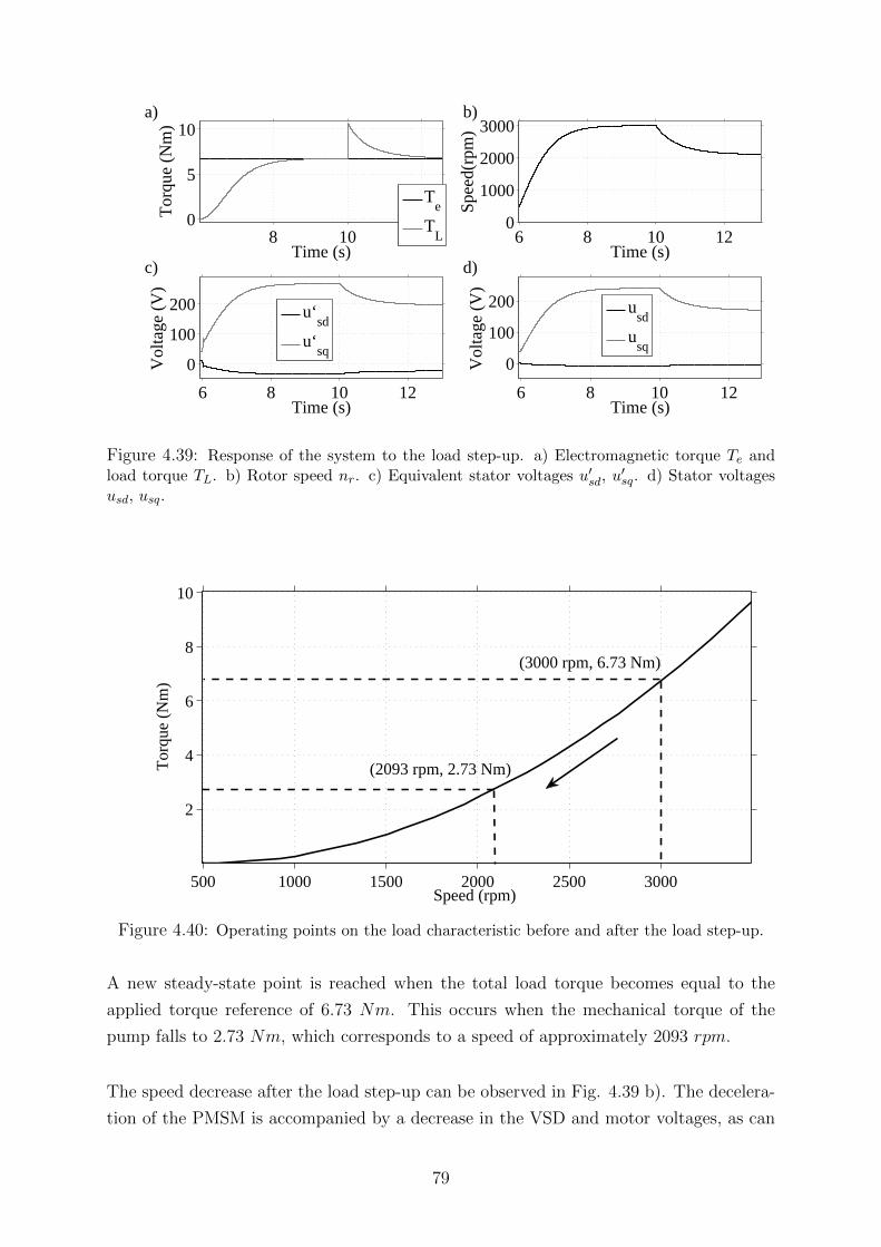
8 10 120

5

10

Time (s)

Tor

que

(Nm

)

a)

Te

TL 6 8 10 12

0

1000

2000

3000

Time (s)

Spee

d(rp

m)

b)

6 8 10 12

0

100

200

Time (s)

Vol

tage

(V

)

c)

u‘sd

u‘sq

6 8 10 12

0

100

200

Time (s)

Vol

tage

(V

)

d)

usd

usq

Figure 4.39: Response of the system to the load step-up. a) Electromagnetic torque Te andload torque TL. b) Rotor speed nr. c) Equivalent stator voltages u′sd, u

′sq. d) Stator voltages

usd, usq.

500 1000 1500 2000 2500 3000

2

4

6

8

10

Speed (rpm)

Tor

que

(Nm

)

(2093 rpm, 2.73 Nm)

(3000 rpm, 6.73 Nm)

Figure 4.40: Operating points on the load characteristic before and after the load step-up.

A new steady-state point is reached when the total load torque becomes equal to the

applied torque reference of 6.73 Nm. This occurs when the mechanical torque of the

pump falls to 2.73 Nm, which corresponds to a speed of approximately 2093 rpm.

The speed decrease after the load step-up can be observed in Fig. 4.39 b). The decelera-

tion of the PMSM is accompanied by a decrease in the VSD and motor voltages, as can

79

be seen in Fig. 4.39 c) and Fig. 4.39 d) respectively.

The obtained results demonstrate that the vector-controlled system responds well to the

applied load increase. The electromagnetic torque and the currents of the motor are not

affected and a new torque balance is achieved through a decrease in the operating speed.

The response of the vector controller to the applied load step-up is clearly better than

the response of both V/f controllers. The presence of relatively large torque and speed

oscillations in the latter cases demonstrates that the performance of V/f control schemes

is more sensitive to load variations.

Load step-down test

In this case, the load torque is stepped down by 4 Nm at 10s and the response of the


8 10 120

2

4

6

Time (s)

Tor

que

(Nm

)

a)

Te

TL

6 8 10 12

1000

2000

3000

Time (s)

Spee

d(rp

m)

b)

8 10 12

0

100

200

300

Time (s)

Vol

tage

(V

)

c)

u‘sd

u‘sq

8 10 120

100

200

300

Time (s)

Vol

tage

(V

)

d)

usd

usq

Figure 4.41: Response of the system to the load step-down. a) Electromagnetic torque Te andload torque TL. b) Rotor speed nr. c) Equivalent stator voltages u′sd, u

′sq. d) Stator voltages

usd, usq.

As in the previous case, the load variation has no observable effect on the currents and

the electromagnetic torque of the motor. The operating point on the load characteristic

changes, according to Fig. 4.42 and a new steady state is reached. The speed of the

PMSM at the new operating point is approximately 3655 rpm.

As can be seen in Fig. 4.41 c) and Fig. 4.41 d), the acceleration of the PMSM results in

an increase in the VSD voltage and the motor voltage respectively. The amplitude of the

80

500 1000 1500 2000 2500 3000 3500 40000

2

4

6

8

10

12

14

Speed (rpm)

Tor

que

(Nm

)(3655 rpm, 10.73 Nm)

(3000 rpm, 6.73 Nm)

Figure 4.42: Operating points on the load characteristic before and after the load step-down.

new steady-state motor voltage is approximately 291.8 V (corresponding to a line-to-line

rms value of 357.4 V , which exceeds the rated voltage of the PMSM).

Since no field-weakening algorithm has been included in this control scheme, it is not

surprising that the motor experiences an overvoltage, when the rotor speed exceeds its

rated value.

4.3.3 Startup performance

The following test demonstrates that the startup of the PMSM is possible, when a vector

controller with a position sensor is used. Moreover, the proper operation of the controller

is verified from the response of the controlled quantities during the startup process.

The mechanical response of the system is presented in Fig. 4.43.

0 1 2 3 40

2

4

6

8

Time (s)

Tor

que

(Nm

)

a)

Te

TL

0 1 2 3 4

1000

2000

3000

Time (s)

Spee

d(rp

m)

b)

Figure 4.43: Mechanical performance during the startup test. a) Electromagnetic torque Teand load torque TL. b) Rotor speed nr.

81

It can be seen from Fig. 4.43 b) that the vector controller manages to accelerate the

PMSM from standstill up to its nominal speed of 3000 rpm within approximately 3s.

The electromagnetic torque reaches its reference value of 6.73 Nm almost instantly, while

the load torque, which is speed-dependent, needs almost 3s to reach this level, as shown

in Fig. 4.43 a).


0 0.2 0.4 0.6−200

0

200

Time (s)

Vol

tage

(V

)

a)

0 0.2 0.4 0.6−10

0

10

Time (s)

Cur

rent

(A

)

b)

0 0.2 0.4 0.6−200

0

200

Time (s)

Vol

tage

(V

)

c)

u‘sd

u‘sq 0 0.005 0.01 0.015 0.02

0

2

4

6

Time (s)

Cur

rent

(A

)

d)

isd

isq

Figure 4.44: VSD voltage and current waveforms during the startup test. a) Equivalent statorvoltages u′sa, u

′sb, u

′sc. b) Stator currents isa, isb, isc. c) Equivalent stator voltages u′sd, u

′sq. d)

Stator currents isd, isq.

The rapid acceleration of the PMSM is reflected in the fast increase of the VSD voltage,

as shown in Fig. 4.44 a). It can be observed in Fig. 4.44 c) that the dominant component

of the supplied voltage is the q-axis component, which indicates high efficiency during

the startup process.

Figure 4.44 b) demonstrates that no overcurrents appear during the startup procedure.

This is expectable, since the d-axis and q-axis currents of the system are directly and

accurately controlled by the implemented PI regulator.

The speed of the current regulation depends on the selected bandwidth of the current

controller. This bandwidth corresponds to a frequency which is selected to be several

times lower than the switching frequency of the VSD.

82

By considering a switching frequency of 7 kHz and by selecting the current controller

to be 10 times slower than the VSD, a bandwidth of approximately 4398 rad/s is obtained.

Although this is the value normally used in this thesis, a lower bandwidth value of 439.8

rad/s has been selected for this test. The lower control speed in this case results in a

higher rise time, which is easier to measure.

According to (3.39), the expected rise time of the controlled currents for the selected

bandwidth is 4.99ms. By measuring the rise time from Fig. 4.44 d), thus by measuring

the time needed by the q-axis current to change from 10% to 90% of its final value, a

time of 5.21ms is obtained. The proximity of the two values indicates that the current

regulator operates properly.


0 0.2 0.4 0.6−200

0

200

Time (s)

Vol

tage

(V

)

a)

0 0.2 0.4 0.6−100

0

100

200

Time (s)

Vol

tage

(V

)

b)

u

sd

usq

Figure 4.45: PMSM voltage waveforms during the startup test. a) Stator voltages usa, usb,usc. b) Stator voltages usd, usq.


transmission system at 0.7s is approximately 17.8% of the VSD voltage. This value

is very low, compared to the observed voltage drops in the performed V/f controlled

startups, which can be attributed to the high efficiency of the vector-controlled startup.


This section presents the simulation results for the implemented position-sensorless vec-

tor controller.

The performance of the controller during and after the control transition is tested and

the response of the system to load disturbances is investigated. Moreover, the behaviour

of the system during field-weakening operation is analyzed and the maximum achievable

speed is determined.

83


For this test, the closed-loop V/f controller is used for the startup of the PMSM and at

6s the control transition takes place. Figure 4.46 presents the performance of the position

estimator after the transition.

6 6.2 6.4 6.60

2

4

6

Time (s)

Ang

le (

rad)

a)

θr

θr,est

6 7 8 9

1000

2000

3000

Time (s)

Spee

d(rp

m)

b)

nr

nr,est

Figure 4.46: Performance of the the position estimator after the control transition. a) Actualposition θr and estimated position θr,est. b) Actual speed nr and estimated speed nr,est.

Figure 4.46 a) shows that an interval of around 0.4s needs to pass, before accurate position

estimates can be produced. The estimated and the actual dq currents during this interval

are shown in Fig 4.47.

6.2 6.4 6.6 6.8 7−6

−4

−2

0

Time (s)

Cur

rent

(A

) a)

isd

isd,est

6.1 6.2 6.3 6.4−4−2

0246

Time (s)

Cur

rent

(A

)

b)

isq

isq,est

Figure 4.47: Actual and estimated currents after the control transition. a) isd and isd,est. b)isq and isq,est.

It can be observed that the initial inability of the controller to produce accurate position

estimates temporarily affects the precision of the performed dq transformations. This

results in significant errors between the actual and the estimated currents during the

initial interval after the transition.

During this interval, the actual d-axis and q-axis currents become negative, which means

that the motor temporarily experiences a reduction in its magnetic flux linkage and a

negative electromagnetic torque. This is demonstrated in Fig. 4.48.

84

6 7 8 9 10

−5

0

5

Time (s)

Tor

que

(Nm

)

a)

Te

TL

6 7 8 9 100.7

0.75

0.8

Time (s)

Flu

x lin

kage

(V

s) b)

ψ‘s,est

Ψm

Figure 4.48: Performance of the system after the control transition. a) Electromagnetic torqueTe and load torque TL. b) Estimated equivalent stator flux linkage ψ′s,est and flux linkage of themagnets Ψm.

Figure 4.48 b) shows that the steady-state value of the estimated flux linkage (0.762 V s)

is slightly higher than the flux linkage of the magnets (0.751 V s). The small difference

between the two values indicates high efficiency, which can be attributed to the zero value

of the commanded d-axis current.

As can be seen in Fig. 4.46 b), the negative electromagnetic torque after the control

transition results in a temporary speed reduction, after which the motor accelerates up

to its target speed of 3000 rpm in less than 3s.

The behaviour of the current regulator after the control transition is shown in Fig. 4.49.

It can be observed that the estimated d-axis and q-axis currents reach their reference

values in less than 20 ms.

6.01 6.02 6.03−3

−2

−1

0

1

Time (s)

Cur

rent

(A

)

a)

isd,est

isd,ref

6.005 6.01 6.015 6.022

4

6

Time (s)

Cur

rent

(A

)

b)

isq,est

isq,ref

Figure 4.49: Estimated stator currents and current references after the control transition. a)isd,est and i∗sd. b) isq,est and i∗sq.

The effect of the control transition on the three-phase voltage waveforms of the VSD and

the motor is shown in Fig. 4.50.

The duration of the voltage oscillations that result from the transition is approximately

85

5.9 5.95 6 6.05 6.1

−50

0

50

Time (s)

Vol

tage

(V

)

a)

0 5 10

0

100

200

300

Time (s)

Vol

tage

(V

)

b)

u‘

sd

u‘sq

5.9 5.95 6 6.05 6.1

−50

0

50

Time (s)

Vol

tage

(V

)

c)

0 5 10

0

100

200

300

Time (s)

Vol

tage

(V

)

d)

u

sd

usq

Figure 4.50: Voltage waveforms during, before and after the control transition. a) Equivalentstator voltages u′sa, u

′sb, u

′sc. b) Equivalent stator voltages u′sd, u

′sq. c) Stator voltages usa, usb,

usc. d) Stator voltages usd, usq.

10 ms. By comparing Fig. 4.50 a) and Fig. 4.50 c), it can be observed that these

oscillations are milder for the motor than for the VSD, thus it can be noticed that the

transmission components act as a filter on the oscillations.

It can be found that the amplitude of the VSD voltage at steady state is approximately

268.7 V , which corresponds to a line-to-line rms value of around 329.1 V .

Similarly, the amplitude of the motor voltage at steady state is approximately 243.1 V ,

(corresponding to a line-to-line rms value of around 297.7 V ), which is roughly equal to

the rated voltage of the PMSM (300 V ).

The steady-state voltage drop in the transmission system is around 9.5% of the VSD

voltage, which is close to the target value of 10%.


This section investigates the response of the position-sensorless controller to load varia-

tions. As usually, the PMSM is subjected to a load step-up and a load step-down test

for this purpose.

86

Load step-up test


the control transition takes place and at 10s the load torque is stepped up by 4 Nm. The

response of the system to the load increase is shown in Fig. 4.51.

6 8 10 12−5

0

5

10

Time (s)

Tor

que

(Nm

)a)

Te

TL

6 8 10 120

2000

4000

Time (s)

Spe

ed(r

pm)

b)

nr

nr,est

6 8 10 12

0

100

200

300

Time (s)

Vol

tage

(V

)

c)

u‘sd

u‘sq

6 8 10 12

0

100

200

300

Time (s)

Vol

tage

(V

)

d)

usd

usq

Figure 4.51: Response of the system to the load step-up. a) Electromagnetic torque Te andload torque TL. b) Actual speed nr and estimated speed nr,est. c) Equivalent stator voltagesu′sd, u

′sq. d) Stator voltages usd, usq.

The electromagnetic torque of the PMSM remains virtually unaffected, as shown in Fig.

4.51 a). Since the total load torque is temporarily higher than the produced electromag-

netic torque, the motor decelerates, as can be seen in Fig. 4.51 b).

The speed decrease causes the pump torque to fall, until a new torque balance is reached

at around 12.8s. The pump torque at the new steady-state point is approximately 2.73

Nm and the corresponding speed is 2093 rpm.

Figures 4.51 c) and d) demonstrate that the q-axis voltages of the VSD and the PMSM

respectively decrease as the motor decelerates. This is expectable, since the the q-axis

voltage component is speed-dependent, according to (3.5).

The performance of the the position estimator after the load step-up is presented in Fig.

4.52. It can be observed that the effect of the sudden load increase on the accuracy of

the position and speed estimation is insignificant.

The behaviour of the current regulator after the load step-up is shown in Fig. 4.53. The

87

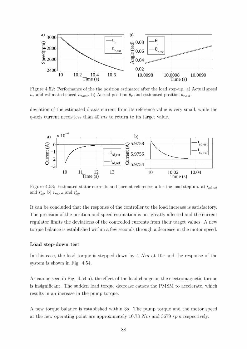
10 10.2 10.4 10.62400

2600

2800

3000

Time (s)

Spee

d(rp

m)

a)

n

r

nr,est

10.0098 10.0098 10.00990.02

0.04

0.06

0.08

Time (s)

Ang

le (

rad)

b)

θ

r

θr,est

Figure 4.52: Performance of the the position estimator after the load step-up. a) Actual speednr and estimated speed nr,est. b) Actual position θr and estimated position θr,est.

deviation of the estimated d-axis current from its reference value is very small, while the

q-axis current needs less than 40 ms to return to its target value.

10 11 12 13−3

−2

−1

0

x 10−4

Time (s)

Cur

rent

(A

)

a)

isd,est

isd,ref

10 10.02 10.04

5.9754

5.9756

5.9758

Time (s)

Cur

rent

(A

)

b)

isq,est

isq,ref

Figure 4.53: Estimated stator currents and current references after the load step-up. a) isd,estand i∗sd. b) isq,est and i∗sq.

It can be concluded that the response of the controller to the load increase is satisfactory.

The precision of the position and speed estimation is not greatly affected and the current

regulator limits the deviations of the controlled currents from their target values. A new

torque balance is established within a few seconds through a decrease in the motor speed.

Load step-down test

In this case, the load torque is stepped down by 4 Nm at 10s and the response of the


As can be seen in Fig. 4.54 a), the effect of the load change on the electromagnetic torque

is insignificant. The sudden load torque decrease causes the PMSM to accelerate, which

results in an increase in the pump torque.

A new torque balance is established within 3s. The pump torque and the motor speed

at the new operating point are approximately 10.73 Nm and 3679 rpm respectively.

88

6 8 10 12−4−2

02468

Time (s)

Tor

que

(Nm

)

a)

Te

TL

6 8 10 120

2000

4000

Time (s)

Spe

ed(r

pm)

b)

nr

nr,est

Figure 4.54: Mechanical response of the system to the load step-down. a) Electromagnetictorque Te and load torque TL. b) Actual speed nr and estimated speed nr,est.

The performance of the the position estimator after the load step-down is presented in

Fig. 4.55. As in the case of the load step-up test, the effect of the load change on the

estimation accuracy appears to be insignificant.

10 10.2 10.4 10.6

31003200330034003500

Time (s)

Spee

d(rp

m)

a)

nr

nr,est

10.0006 10.0007 10.00083.45

3.46

3.47

3.48

Time (s)

Ang

le (

rad)

b)

θr

θr,est

Figure 4.55: Performance of the the position estimator after the load step-down. a) Actualspeed nr and estimated speed nr,est. b) Actual position θr and estimated position θr,est.

Since the load decrease causes the rotor speed to exceed its rated value, the PMSM enters

the field-weakening mode, as demonstrated in Fig. 4.56.

9 10 11 12

−8−6−4−2

0

Time (s)

Cur

rent

(A

)

a)

9 10 11 12

0.65

0.7

0.75

0.8

Time (s)

Flu

x lin

kage

(V

s) b)

ψ‘s,est

Ψm

Figure 4.56: Field-weakening operation after the load step-down. a) Estimated d-axis currentisd,est. b) Estimated equivalent stator flux linkage ψ′s,est and flux linkage of magnets Ψm.

89

After the field-weakening algorithm is activated, a negative magnetizing current is com-

manded. This causes the d-axis stator current to reach a negative value of approximately

7.95 A, which results in a decrease in the equivalent stator flux linkage. As shown in Fig.

4.56 b), the flux linkage falls from 0.762 V s to 0.636 V s.

The existence of the field-weakening algorithm allows the PMSM to operate above its

rated speed, without experiencing voltage values that exceed its rated voltage. This is

demonstrated in Fig. 4.57.

6 8 10 12−100

0

100

200

300

Time (s)

Vol

tage

(V

)

a)

u‘sd

u‘sq

6 8 10 12−100

0

100

200

300

Time (s)

Vol

tage

(V

)

b)

usd

usq

6 8 10 120

200

Time (s)

Vol

tage

(V

)

c)

u‘s,max

us,max

6 8 10 120

5

10

Time (s)

Cur

rent

(A

)

d)

Figure 4.57: Voltage and current waveforms before and after the load step-down. a) Equivalentstator voltages u′sd, u

′sq. b) Stator voltages usd, usq. c) Amplitude of the equivalent stator voltage

u′s and of the stator voltage us. d) Amplitude is of the stator current.

A speed rise without field-weakening would normally be accompanied by an increase of

the q-axis component of the motor voltage. In our case however, this component remains

almost constant, while the magnitude of the d-axis voltage rises slightly, as a result of

the increased magnitude of the magnetizing current.

Figure 4.57 c) demonstrates that, thanks to the field-weakening algorithm of the con-

troller, the amplitude of the motor voltage remains close to its rated value after the load

decrease.

However, the amplitude of the stator current increases substantially, as a result of the

increase in the magnitude of the commanded magnetizing current. As shown in Fig. 4.57

d), the current amplitude rises from 5.98 A (which corresponds to an rms value of 4.23

A) to 9.97 A (which corresponds to an rms value of 7.05 A).

90

The current rise also causes an increase in the voltage drop in the transmission system,

which, in turn, results in an increase in the voltage amplitude of the VSD.

As shown in Fig. 4.57 c), the amplitude of the supplied voltage rises from 268.8 V (which

corresponds to a line-to-line rms value of 329.2 V ) to 279.5 V (which corresponds to a

line-to-line rms value of 342.3 V ).

The voltage drop in the transmission system, which is approximately 9.5% of the VSD

voltage before the load decrease, increases to 11% of the VSD voltage after the load step-

down.

The resistive losses for the two operating points can be calculated, by considering the

equivalent resistance R′s of the system (which is approximately equal to 5.16 Ω for the

selected cable length) and the current magnitude in the two cases.

It can be found that the resistive losses are approximately 276.7 W before the load step-

down. When the new steady-state point is established, the resistive losses rise to almost

768.8 W . The loss increase in this case accounts for more than 177% of the losses during

rated-speed operation, while the corresponding speed increase is only 23% of the rated

speed.

The obtained results demonstrate that a speed increase by means of field-weakening

comes at the cost of an increased voltage drop in the transmission components and

significantly increased resistive losses. The field-weakening capability of the system is

further investigated in Section 4.4.3.

4.4.3 Field-weakening performance

This section evaluates the possibility of extending the speed range of the PMSM, by

applying the implemented field-weakening strategy. The maximum speed that can be

reached is determined and the performance of the system at the corresponding operating

point is investigated.

The field-weakening mode can be activated either through a decrease in the load torque

(as in the case of the load step-down test in Section 4.4.2), or through an increase in the

commanded torque.

91

In order to determine the highest speed that can be achieved for the considered pump

load, it is sufficient to set a high reference torque, which forces the motor to operate at

its rated current.

The current limiter that has been included in the vector controller prevents the stator

current from exceeding its rated value. This sets the limit for the maximum electromag-

netic torque that can be produced and, through the load characteristic, for the maximum

speed that can be reached.

Determination of maximum achievable speed

For the following test, the closed-loop V/f controller is used for the startup of the PMSM

and at 6s the position-sensorless vector controller is deployed.

The torque reference is initially set equal to the value of the load torque that corresponds

to the nominal speed of the PMSM (6.73 Nm). At 10s, the commanded torque is doubled

and the response of the system is presented in Fig. 4.58.

8 9 10 11 12−10

0

10

Time (s)

Cur

rent

(A

)

a)

isd

isq

8 9 10 11 125

10

Time (s)

Cur

rent

(A

)

b)

8 9 10 11 122500

3000

3500

Time (s)

Spe

ed(r

pm)

c)

nr

nr,est 8 9 10 11 12

5

10

Time (s)

Tor

que

(Nm

)d)

Te

TL

Figure 4.58: Response of the system to the torque reference step-up. a) Stator currents isd,isq. b) Amplitude is of the stator current. c) Actual speed nr and estimated speed nr,est. d)Electromagnetic torque Te and load torque TL.

The large increase in the ordered torque causes the q-axis current reference to exceed the

rated current of the PMSM. The high commanded current results in the activation of

the current limiter and the limitation of the q-axis current to the value of 11.31A (which

corresponds to the rated rms current of 8 A).

92

As a result of the current limitation, the produced electromagnetic torque cannot be

doubled, as commanded, but is limited to a value of approximately 12.75 Nm at 10s, as

can be seen in Fig. 4.58 d).

The speed-dependent load torque cannot follow the almost instant increase of the elec-

tromagnetic torque. The resulting torque difference causes the PMSM to accelerate, as

can be seen in Fig. 4.58 c).

Since the rotor speed exceeds its rated value, the field-weakening mode is entered, thus

a negative d-axis current is ordered. As the speed increases, the magnitude of the com-

manded d-axis current increases as well (thus the magnetizing current becomes ’more

negative’), as shown in Fig. 4.58 a).

As the magnitude of the d-axis reference current increases, the current limiter forces the

commanded q-axis current to decrease, so that the overall stator current does not exceed

its rated value. This causes the produced electromagnetic torque to decrease during the

acceleration of the PMSM.

As shown in Fig. 4.58 d), as the rotor speed increases, the load torque increases too and a

new torque balance is established at around 11.1s. The torque that the PMSM produces

at the new steady-state point is approximately 9.88 Nm.

As can be seen in Fig. 4.58 c), the speed at the new operating point is approximately 3529

rpm. Apparently, this is the maximum speed that can be reached, without exceeding the

rated current of the motor for the considered pump load.

The back-EMF amplitude, being proportional to the speed of the PMSM, also takes its

maximum value at the new steady-state point. From Fig. 4.59 a), this value is found to

be approximately 277.7 V (corresponding to a line-to-line rms voltage of 340.1 V ).

As was discussed in Section 3.6.6, if the stator current is suddenly lost for some reason,

the back-EMF of the PMSM will fall on the output of the VSD. In order to avoid dam-

aging the drive, it is necessary for the inverter to be capable of handling the maximum

back-EMF amplitude.

As can be seen in Fig. 4.59 a), the maximum back-EMF amplitude in the studied case

(277.7 V ) is lower than the voltage amplitude that the VSD output normally experi-

ences during maximum-speed operation (approximately 291.7 V ). Therefore, handling

93

8 9 10 11 12200

250

300

350

Time (s)

Vol

tage

(V

)

a)

u‘s,max

emax

9 10 11 12

0.65

0.7

0.75

0.8

Time (s)

Flux

link

age

(Vs)

b)

ψ‘s,est

Ψm

Figure 4.59: Response of the system to the torque reference step-up. a) Amplitude of theequivalent stator voltage u′s and of the back-EMF e. b) Estimated equivalent stator fluxlinkage ψ′s,est and flux linkage of magnets Ψm.

this back-EMF should be no problem for the inverter.

Figure 4.59 b) shows that the amplitude of the estimated flux linkage ψ′s,est falls to ap-

proximately 0.665 V s after the torque reference step-up. Apparently, this is the minimum

value that can be reached for the considered load.

Figure 4.58 b) demonstrates that the step-up of the torque reference at 10s results in an

increase in the stator current magnitude up to the value of 11.31 A (which corresponds

to the rated rms current of 8 A).

Although the composition of the stator current changes as the motor accelerates (as

shown in Fig. 4.58 a)), its amplitude after the torque increase remains constant and

equal to its maximum acceptable value.

Efficiency calculations and comparisons

The implemented field-weakening algorithm allows the motor to operate at high speeds,

without experiencing any overvoltages.

The performed torque reference step-up test demonstrated that a maximum speed of

approximately 3529 rpm can be reached and a maximum steady-state torque of around

9.88 Nm can be produced by the PMSM during field-weakening operation.

During the load step-down test in Section 4.4.2, it was demonstrated that even higher

speeds can be reached, when lighter loads are considered. The speed that was obtained

during that test was around 3679 rpm.

However, for the current analysis, the pump load that was introduced in Section 4.1.1

94

is considered. In this case, field-weakening can extend the speed range of the PMSM by

approximately 17.6% and can result in a 46.8% increase in the produced electromagnetic

torque.

It is important to note, however, that the aforementioned enhancement in the mechanical

performance of the motor is achieved through a 89.2% increase in the magnitude of the

stator current. The increased current results in higher losses and a larger voltage drop in

the transmission system.

The total resistive losses are approximately 276.7 W , when the PMSM operates at its

rated speed, while they rise to almost 990.2 W during maximum-speed operation. This

corresponds to a loss increase of more than 257%.

These loss calculations have been performed by considering the same equivalent resis-

tance R′s for both operating points. However, by taking into account that the increased

losses cause higher temperatures, which in turn increase the resistances of the motor and

the transmission components, the loss increase should be expected to be even greater.

The overall efficiency of the system in the cases of rated-speed operation and maximum-

speed operation can be obtained, by calculating the input and output power values for

both operating points. The system considered in these calculations includes the motor

and the transmission components.

The input power of the system can be calculated from the voltage and current waveforms

at the output of the VSD, according to (3.25). The power factor in this relation is ob-

tained from the phase difference between the voltage and current.

On the other hand, the output power of the system, thus the mechanical power of the

PMSM, can be readily calculated as the product of the load torque and the mechanical

speed of the motor.

In the case of rated-speed operation, the VSD voltage and current amplitudes are 268.8

V and 5.98 A respectively and the power factor angle is approximately 5.6o. This yields

an input power value of 2399 W . The output power, calculated for a load torque of 6.73

Nm and a speed of 314.2 rad/s (corresponding to 3000 rpm), is approximately equal to

2114 W .

By subtracting the output from the input power, the total power losses in the case of

95

rated-speed operation are found to be 285 W . This value is in good agreement with the

total resistive losses calculated earlier (276.7 W ). The efficiency of the system in this

case is almost 88.1%.

In the case of maximum-speed operation, the VSD voltage and current amplitudes are

291.7 V and 11.31 A respectively and the power factor angle is roughly 20.1o. The re-

sulting input power is almost 4647 W . The output power, calculated for a load torque

of 9.88 Nm and a speed of 369.6 rad/s (corresponding to 3529 rpm), is approximately

equal to 3652 W .

The total power losses in the case of maximum-speed operation can be found to be 995

W . Once again, this value is very close to the resistive losses calculated earlier (990.2

W ). The efficiency of the system in this case falls to almost 78.5%.

Apart from the decreased efficiency during field-weakening operation, the increased cur-

rent magnitude also causes a larger voltage drop in the transmission system. While the

drop is around 9.5% of the VSD voltage during rated-speed operation, it rises up to

approximately 14.7% during maximum-speed operation.

96

Chapter 5

Experimental results

This chapter presents the obtained experimental results and describes the laboratory

topology on which the presented measurements have been performed.

Initially, the small-scale lab model of the studied system is described and the control and

monitoring topologies are introduced.

The performance of the V/f controller of the VSD is then investigated both during the

startup of the system and during steady-state operation of the PMSM. In both cases, the

measurements are performed for two different loads.

Finally, the behaviour of the system under position-sensorless vector control is tested

after the transition from V/f control, after sudden variations of the load torque and after

changes of the torque reference. The performance of the field-weakening algorithm of the

vector controller is also investigated during operation at relatively high speeds.

5.1 Experimental setup

This section describes the experimental setup on which the presented measurements have

been performed. As shown in Fig. 5.1, this setup includes the model of the investigated

system, the monitoring topology and the control system of the drive.

The setup of the small-scale system model and the implementation of the VSD control

through the drive software have not been parts of this thesis. On the other hand, the

preparation of the data acquisition code in LabVIEW and the configuration of the Com-

pactRIO device have been in the scope of this work.

The implemented data acquisition system, consisting of the CompactRIO device and the

97

LabVIEW code, has been used to monitor the electrical quantities of the PMSM. On the

other hand, in order to measure the VSD quantities and to obtain the estimated speed

and torque waveforms of the PMSM, the monitoring capabilities of the drive have been

utilized.

M PTransmission

system modelVSD

Power source

PMSM Pump model

Drive software

Setup of control

configuration

CompactRIO

LabVIEW

Current and voltage

measurements

Data acquisition

Figure 5.1: Layout of the experimental setup, consisting of the system model, the monitoringtopology and the control system.

5.1.1 Small-scale laboratory model

The considered laboratory system is a small-scale model of the offshore system that is

investigated in this thesis. The setup of this model has not been conducted during this

thesis, but was implemented as part of a previous work [1].

As shown in Fig. 5.1, the laboratory model includes a power source, a VSD, a model of

the transmission system, a PMSM and a model of the multiphase pump.

As shown in Fig. 5.2, the model of the transmission system is composed of two 1:1

transformers and a cable simulator, all connected in series with each other. The cable

simulator consists of an electric circuit in which the cable parameters are distributed over

a number of series-connected π-equivalent elements.

The pump model represents the mechanical load of the system and consists of a per-

manent magnet generator, a flywheel, a break-away torque device and three identical

adjustable resistors, as demonstrated in Fig. 5.3.

98

Cable simulator

1:1 transformer 1:1 transformer

PMSMVSD

Figure 5.2: Layout of the transmission system model, consisting of two 1:1 transformers and acable simulator.

G

PMSG

M

PMSM

Break-away torque

mechanism

FlywheelResistive load

Figure 5.3: PMSM and pump model assembly, consisting of a PMSG, a flywheel, a break-awaytorque mechanism and a resistive load.

The generator is mechanically coupled to the motor, while the flywheel and the break-

away torque mechanism are attached on the common shaft of the assembly. The mission

of the flywheel is to increase the inertia of the system, while the aim of the break-away

torque device is to simulate the break-away torque of the actual multiphase pump.

The resistors are connected to the stator windings of the permanent magnet generator as

a symmetrical three-phase electrical load.

When the motor-generator assembly rotates, a voltage is induced at the stator windings

of the generator and a current flows through the resistive load. This current results in an

electromagnetic torque that opposes the torque produced by the PMSM and, therefore,

acts as a load torque for the motor.

By assuming almost 100% efficiency for the PMSG, thus by considering that its electric

power output pe,gen is almost equal to its mechanical power input pm, the load torque of

the motor can be obtained from

pm ' pe,gen ⇒ TLωrnp' 3

2

u2s,genRgen

' 3

2

ω2r ψ

2s,gen

Rgen

⇒ TL '3

2

npψ2s,gen

Rgen

ωr (5.1)

99

where Rgen is the per-phase load resistance and us,gen and ψs,gen are the amplitudes of

the stator voltage and the stator flux linkage of the generator respectively.

When the speed of the PMSM does not exceed its rated value, thus when the motor does

not operate in field-weakening mode, the amplitude ψs,gen of the stator flux linkage can

be considered to be speed-independent. Therefore, according to (5.1), the load torque

can be considered to be approximately proportional to the speed of the motor.

Since (5.1) is based on (3.14), it assumes that the stator flux linkage of the generator is

constant and that the voltage drop in its stator resistance is negligible. Therefore, the

derived load torque expression is approximate.

5.1.2 Control and monitoring system

The PMSM of the laboratory model is controlled by the VSD through the transmission

system. The VSD control is set up by dedicated drive software, which runs on a computer

that is directly connected to the VSD.

The drive software allows the PMSM to be controlled in different ways and offers several

monitoring possibilities. The setup of the V/f control and vector control configurations

in this software has not been part of this thesis.

Two current flukes and two voltage probes were used during the performed experiments,

in order to obtain measurements of two motor currents and two motor voltages respec-

tively.

In order to collect and store the measured data, the measuring units were connected

to the analog inputs of a NI CompactRIO device, which, in turn, was connected to a

computer. The configuration of the CompactRio device and the development of the data

acquisition code in LabVIEW has been performed in the framework of this thesis.

The developed LabVIEW code acquires the measurements from the CompactRIO input

modules at a sufficient rate and stores them in the memory of the device. It also performs

real-time monitoring, thus it allows the current and voltage waveforms to be shown on

the screen of the computer during the execution of the experiments.

100

5.2 V/f control

The measurements that have been obtained during scalar-controlled operation of the

system are presented in this section. The performance of the V/f controller is investigated

under two different loads, both during the startup of the system and during steady-state

operation of the motor.

5.2.1 Startup performance

An open-loop V/f controller is used for the startup of the PMSM and its performance

is studied by monitoring and analyzing the currents and voltages of the VSD and the

PMSM.

In order to obtain the drive measurements, the monitoring capabilities of the VSD have

been utilized, while the motor measurements have been obtained with the implemented

monitoring system, which is based on LabVIEW and CompactRIO.

Startup under full load

For the following startup tests, the load resistance Rgen is set equal to its minimum

available value (Rgen = 27 Ω), which, according to (5.1), corresponds to the maximum

achievable load torque TL.

The V/f controller is used to accelerate the motor from standstill up to a specified target

speed. The startup procedure is repeated for different initial rotor positions, which are

randomly selected, and the waveforms of the drive current are presented in Fig. 5.4.

It can be observed that the initial current of the drive is relatively high, which can be

attibuted to the static load torque of the system and to the magnetization of the two

transformers.

The waveforms of the voltage references that are produced by the drive are presented

in Fig. 5.5. Since the VSD uses an open-loop V/f control scheme for the startup of

the motor, the commanded voltage is not affected by the actual response of the system.

Therefore, the voltage reference waveforms are very similar in all tested cases.

During the performed tests, the voltage output of the VSD is not filtered. According to

the discussion in Section 2.2.2, the absence of a filter is expected to result in the presence

of high-order harmonics in the voltage that is supplied to the motor. Indeed, this can be

101

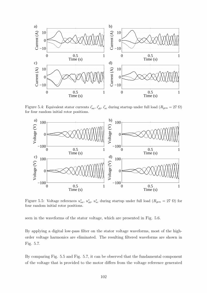
0 0.5 1

−10

0

10

Time (s)

Cur

rent

(A

)

a)

0 0.5 1

−10

0

10

Time (s)

Cur

rent

(A

)

b)

0 0.5 1

−10

0

10

Time (s)

Cur

rent

(A

)

c)

0 0.5 1

−10

0

10

Time (s)

Cur

rent

(A

)

d)

Figure 5.4: Equivalent stator currents i′sa, i′sb, i

′sc during startup under full load (Rgen = 27 Ω)

for four random initial rotor positions.

0 0.5 1−100

0

100

Time (s)

Vol

tage

(V

)

a)

0 0.5 1−100

0

100

Time (s)

Vol

tage

(V

)

b)

0 0.5 1−100

0

100

Time (s)

Vol

tage

(V

)

c)

0 0.5 1−100

0

100

Time (s)

Vol

tage

(V

)

d)

Figure 5.5: Voltage references u∗sa, u∗sb, u

∗sc during startup under full load (Rgen = 27 Ω) for

four random initial rotor positions.

seen in the waveforms of the stator voltage, which are presented in Fig. 5.6.

By applying a digital low-pass filter on the stator voltage waveforms, most of the high-

order voltage harmonics are eliminated. The resulting filtered waveforms are shown in

Fig. 5.7.

By comparing Fig. 5.5 and Fig. 5.7, it can be observed that the fundamental component

of the voltage that is provided to the motor differs from the voltage reference generated

102

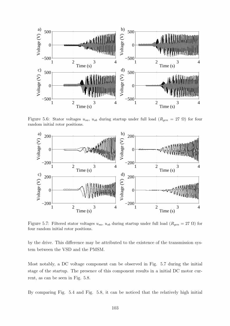
1 2 3 4−500

0

500

Time (s)

Vol

tage

(V

)

a)

1 2 3 4−500

0

500

Time (s)

Vol

tage

(V

)

b)

1 2 3 4−500

0

500

Time (s)

Vol

tage

(V

)

c)

1 2 3 4−500

0

500

Time (s)

Vol

tage

(V

)

d)

Figure 5.6: Stator voltages usa, usb during startup under full load (Rgen = 27 Ω) for fourrandom initial rotor positions.

1 2 3 4−200

0

200

Time (s)

Vol

tage

(V

)

a)

1 2 3 4−200

0

200

Time (s)

Vol

tage

(V

)

b)

1 2 3 4−200

0

200

Time (s)

Vol

tage

(V

)

c)

1 2 3 4−200

0

200

Time (s)

Vol

tage

(V

)

d)

Figure 5.7: Filtered stator voltages usa, usb during startup under full load (Rgen = 27 Ω) forfour random initial rotor positions.

by the drive. This difference may be attributed to the existence of the transmission sys-

tem between the VSD and the PMSM.

Most notably, a DC voltage component can be observed in Fig. 5.7 during the initial

stage of the startup. The presence of this component results in a initial DC motor cur-

rent, as can be seen in Fig. 5.8.

By comparing Fig. 5.4 and Fig. 5.8, it can be noticed that the relatively high initial

103

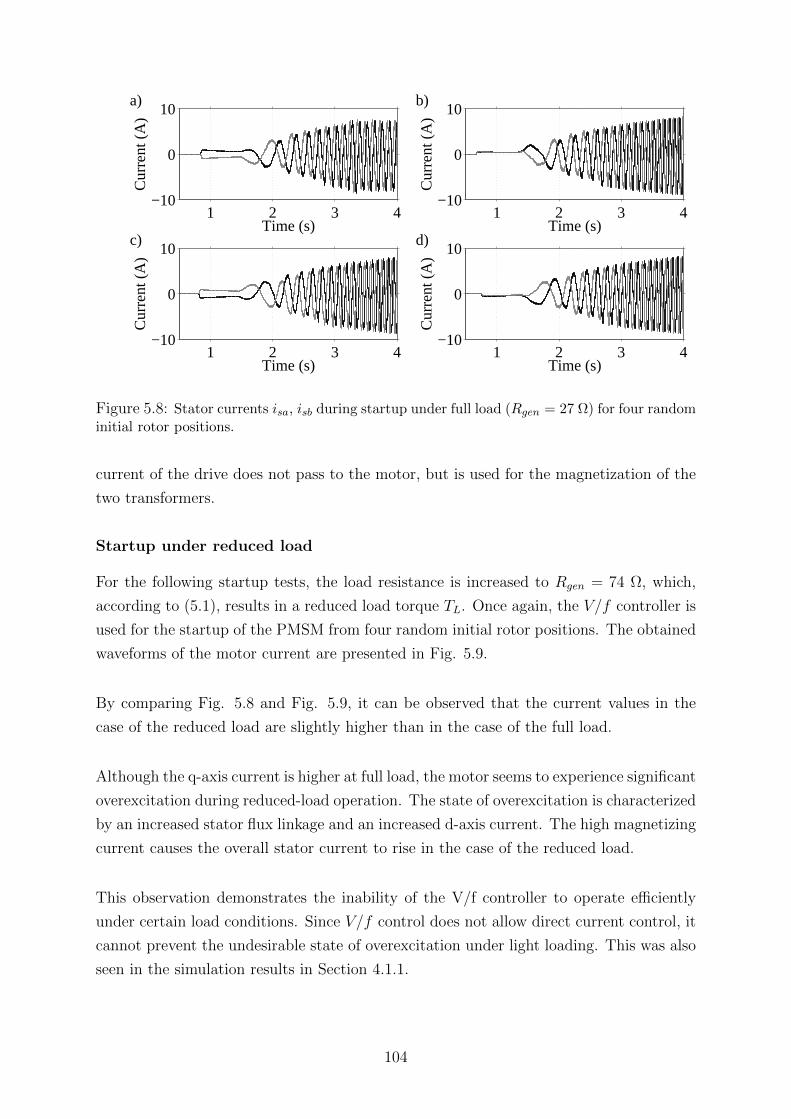
1 2 3 4−10

0

10

Time (s)

Cur

rent

(A

)

a)

1 2 3 4−10

0

10

Time (s)

Cur

rent

(A

)

b)

1 2 3 4−10

0

10

Time (s)

Cur

rent

(A

)

c)

1 2 3 4−10

0

10

Time (s)

Cur

rent

(A

)

d)

Figure 5.8: Stator currents isa, isb during startup under full load (Rgen = 27 Ω) for four randominitial rotor positions.

current of the drive does not pass to the motor, but is used for the magnetization of the

two transformers.

Startup under reduced load

For the following startup tests, the load resistance is increased to Rgen = 74 Ω, which,

according to (5.1), results in a reduced load torque TL. Once again, the V/f controller is

used for the startup of the PMSM from four random initial rotor positions. The obtained

waveforms of the motor current are presented in Fig. 5.9.

By comparing Fig. 5.8 and Fig. 5.9, it can be observed that the current values in the

case of the reduced load are slightly higher than in the case of the full load.

Although the q-axis current is higher at full load, the motor seems to experience significant

overexcitation during reduced-load operation. The state of overexcitation is characterized

by an increased stator flux linkage and an increased d-axis current. The high magnetizing

current causes the overall stator current to rise in the case of the reduced load.

This observation demonstrates the inability of the V/f controller to operate efficiently

under certain load conditions. Since V/f control does not allow direct current control, it

cannot prevent the undesirable state of overexcitation under light loading. This was also

seen in the simulation results in Section 4.1.1.

104

0.5 1 1.5 2 2.5 3

−10

0

10

Time (s)

Cur

rent

(A

)

a)

3 3.5 4 4.5 5 5.5

−10

0

10

Time (s)

Cur

rent

(A

)

b)

1.5 2 2.5 3 3.5 4

−10

0

10

Time (s)

Cur

rent

(A

)

c)

0.5 1 1.5 2 2.5 3

−10

0

10

Time (s)

Cur

rent

(A

)

d)

Figure 5.9: Stator currents isa, isb during startup under reduced load (Rgen = 74 Ω) for fourrandom initial rotor positions.

As in the case of the full load, a DC current component can be seen in Fig. 5.9 during

the initial stage of the startup. The DC current is the result of a similar component in

the motor voltage, as can be seen in the filtered voltage waveforms of Fig. 5.10.

1.5 2 2.5 3 3.5−200

0

200

Time (s)

Vol

tage

(V

)

a)

2 3 4−200

0

200

Time (s)

Vol

tage

(V

)

b)

1 2 3 4−200

0

200

Time (s)

Vol

tage

(V

)

c)

1.5 2 2.5 3 3.5 4−200

0

200

Time (s)

Vol

tage

(V

)

d)

Figure 5.10: Filtered stator voltages usa, usb during startup under reduced load (Rgen = 74 Ω)for four random initial rotor positions.

105

5.2.2 Steady-state operation

For the following tests, the V/f controller is used to accelerate the PMSM from standstill

up to different target speeds. The steady-state values of the equivalent stator voltage

amplitude u′s and the stator current amplitude is are measured at six different speeds

and under two different loading conditions and are presented in Table 5.1 and Table 5.2.

Table 5.1: Steady-state measurements for operation under full load (Rgen = 27 Ω).

Rotor speed nr (rpm) 500 1000 1500 2000 2500 3000

Voltage amplitude u′s (V) 57.1 109.9 164.5 222.0 278.5 318.3

Current amplitude is (A) 7.9 9.9 10.5 10.9 11.9 12.4

Table 5.2: Steady-state measurements for operation under reduced load (Rgen = 74 Ω).

Rotor speed nr (rpm) 500 1000 1500 2000 2500 3000

Voltage amplitude u′s (V) 57.2 109.1 164.3 216.7 271.7 325.4

Current amplitude is (A) 8.2 10.3 11.8 11.9 12.5 12.4

Both tables demonstrate that the voltage amplitude produced by the drive is almost pro-

portional to the commanded rotor speed, which is not surprising according to (3.53).

Moreover, it can be observed that the current amplitude increases for higher rotor speeds.

According to (5.1), the load torque rises when the speed increases, causing an increase

in the torque-producing component of the equivalent stator current and therefore an in-

crease in the overall stator current.

By comparing Table 5.1 and Table 5.2, it can also be noticed that the current values in

the case of the full load are lower than in the case of the reduced load. As was discussed

in Section 5.2.1, this result can be attributed to the high d-axis current that the motor

experiences under light loading.


This section presents the measurements that have been obtained during vector-controlled

operation of the system. In the performed tests, the V/f controller is used for the initial

acceleration of the PMSM and the position-sensorless vector controller is activated after

a certain speed is reached.

106

Initially, the behaviour of the system is studied after the transition from scalar to vector

control. Different torque reference values are used for the vector controller and the tests

are repeated with the field-weakening algorithm both activated and deactivated.

The performance of the vector controller after load variations is then tested, by sub-

jecting the PMSM to sudden load increases and decreases. These tests verify that the

controlled quantities stay close to their reference values after load disturbances and that

the field-weakening mode is entered successfully, when a certain speed is exceeded.

Finally, the performance of the system after sudden torque reference variations is tested,

by commanding a rotation reversal, thus by changing the sign of the applied torque

reference. This test verifies that the controller responds properly to changes in the ordered

torque and that the transition from vector to scalar control and vice versa is performed

successfully at low speeds during the reversal.


For the following tests, the V/f controller is used to accelerate the PMSM from standstill

up to 250 rpm. After a few seconds of steady-state operation at this speed, the control

transition takes place, thus the V/f controller is dismissed and the vector controller is

deployed.

Initially, the behaviour of the system during the transition is investigated for two different

cases. In both cases, the torque reference that is provided to the vector controller is 10

Nm. However, in the first case, the field-weakening function of the drive is deactivated,

while in the second one, it is activated when the speed of the PMSM becomes higher

than 2400 rpm.

Furthermore, the response of the system after the transition is obtained for different

torque reference values and the measured motor currents are used to verify that the

vector controller operates properly.

Test without field-weakening

The behaviour of the system during the control transition, when no field-weakening op-

eration is considered, is shown in Fig. 5.11.

It be seen in Fig. 5.11 d) that the estimated electromagnetic torque of the motor during

V/f control is approximately equal to 5.5 Nm. After the transition, the torque increases

107

4 6 80

1000

2000

3000

Time (s)

Spee

d (r

pm)

a)

4 6 84

6

8

Time (s)

Cur

rent

(A

)

b)

4 6 80

200

400

Time (s)

Vol

tage

(V

)

c)

4 6 80

5

10

Time (s)

Tor

que

(Nm

)

d)

Figure 5.11: Control transition with the field-weakening function deactivated. a) Estimatedrotor speed nr,est. b) Equivalent stator current magnitude i′s. c) Equivalent stator voltagemagnitude u′s. d) Estimated electromagnetic torque Te,est.

to its reference value of 10 Nm.

Figure 5.11 b) shows that the magnitude of the VSD current before the transition is

around 4.9 A, while, after the transition, it becomes approximately equal to 5.9 A.

It can be noticed that although the produced torque is almost 81.8% higher in the case

of vector control, the respective increase in the current magnitude is only 20.4%. This

demonstrates that much higher torque-to-current ratios can be achieved with vector con-

trol.

Figure 5.11 a) shows that after the transition, the estimated rotor speed increases rapidly

from 250 rpm to the steady-state value that corresponds to the commanded torque (2620

rpm).

It can be seen in Fig. 5.11 c) that the speed rise is accompanied by an increase in the

VSD voltage magnitude. The steady-state value of the voltage magnitude is approxi-

mately equal to 290 V .

On the other hand, Fig. 5.11 b) shows that the VSD current magnitude remains constant,

since the d-axis and q-axis current references in the vector controller are also constant.

108

Test with field-weakening

The previous test is performed again, but this time the field-weakening function is ac-

tivated when the speed exceeds the specified value of 2400 rpm. The behaviour of the

system in this case is shown in Fig. 5.12.

4 6 80

1000

2000

3000

Time (s)

Spee

d (r

pm)

a)

4 6 84

6

8

Time (s)

Cur

rent

(A

)

b)

4 6 80

200

400

Time (s)

Vol

tage

(V

)

c)

4 6 80

5

10

Time (s)

Tor

que

(Nm

)

d)

Figure 5.12: Control transition with the field-weakening function activated. a) Estimated rotorspeed nr,est. b) Equivalent stator current magnitude i′s. c) Equivalent stator voltage magnitudeu′s. d) Estimated electromagnetic torque Te,est.

Figure 5.12 d) demonstrates that the estimated electromagnetic torque after the transi-

tion remains constant and equal to its reference value.

As shown in Fig. 5.12 c), the speed rise after the transition is initially achieved through

an increase in the voltage magnitude of the VSD. However, when the specified speed value

of 2400 rpm is reached at approximately 5.5s, the field-weakening function is activated

and the voltage magnitude stops increasing.

During the field-weakening operation, a negative d-axis current of increasing magnitude

is commanded. This causes a further speed rise after 5.5s, as can be seen in Fig. 5.12 a),

but also an increase in the magnitude of the overall VSD current, as shown in Fig. 5.12

b).

Different torque reference values

Next, the performance of the vector controller is tested for different values of the applied

torque reference. The waveforms of two measured phase currents during the control tran-

109

sition are shown in Fig. 5.13 for three different torque reference values.

5.5 6 6.5−10

0

10

Time (s)

Cur

rent

(A

)a)

7 7.5−10

0

10

Time (s)

Cur

rent

(A

)

b)

4.5 5 5.5−10

0

10

Time (s)

Cur

rent

(A

)

c)

Figure 5.13: Stator currents isa, isb for different torque reference values. a) T ∗e = 5 Nm. b)T ∗e = 8 Nm. c) T ∗e = 10 Nm.

Figure 5.13 demonstrates that the control transition is followed by a short interval of

current oscillations. These oscillations last for less than 1s and, as in the case of the

performed simulations, they might result from inaccurate position estimation during the

initial interval of the vector-controlled operation.

Since no field-weakening operation is considered, the d-axis current of the motor is ex-

pected to be almost zero after the transition, which means that the amplitude of the total

stator current is expected to be approximately equal to the q-axis current component.

By using (3.29), the expected stator current amplitude can be calculated for different

values of the applied torque reference. The results obtained for 5 Nm, 8 Nm and 10

Nm are approximately 4.4 A, 7.1 A and 8.9 A respectively. These values are close to the

current amplitudes after the control transition in Fig. 5.13.


The aim of the following tests is to study the response of the system to load variations

during vector-controlled operation.

According to (5.1), the load torque of the PMSM can be changed, by varying the resis-

tance Rgen of the PMSG. In order to achieve a load step-down, the resistance in all three

phases is suddenly increased, while a load step-up is obtained through a sudden decrease

of the resistance.

For the following tests, the system is ordered to operate in the field-weakening mode,

when the speed of the PMSM exceeds the selected value of 2400 rpm.

110

Load step-down test

For this test, the system operates under vector control with an applied torque reference

of 5Nm. At 4.7s, a load step-down is applied by increasing the value of the per-phase

resistance Rgen from 27 Ω to 74 Ω. The response of the system is shown in Fig. 5.14.

4 6 8 10

1000

2000

3000

Time (s)

Spee

d (r

pm)

a)

4 6 8 10

2

4

6

Time (s)

Cur

rent

(A

)

b)

4 6 8

100

200

300

Time (s)

Vol

tage

(V

)

c)

4 6 8 10

2

4

6

8

Time (s)

Tor

que

(Nm

)

d)

Figure 5.14: Response of the system to a load step-down. a) Estimated rotor speed nr,est.b) Equivalent stator current magnitude i′s. c) Equivalent stator voltage magnitude u′s. d)Estimated electromagnetic torque Te,est.

As shown in Fig. 5.14 d), the electromagnetic torque of the motor does not deviate

from its reference value (5 Nm). The resulting torque inbalance after the load step-down

causes the motor to accelerate, as shown in Fig. 5.14 a).

The acceleration stops when a new torque balance is established, thus when the load

torque becomes equal to the electromagnetic torque of the motor (which is approximately

equal to the applied reference torque).

The field-weakening mode is entered around 7.2s, when the speed of the motor exceeds

the selected value of 2400 rpm. At this point, the voltage increase stops, as shown in Fig.

5.14 c), and further acceleration is enabled by a negative d-axis current, which increases

the magnitude of the total stator current, as shown in Fig. 5.14 b).

Load step-up test

In this case, a load step-up is applied by decreasing the value of the per-phase resistance

Rgen from 74 Ω to 27 Ω at 6.8s. The response of the system is shown in Fig. 5.15.

111

2 4 6 8 100

1000

2000

3000

Time (s)

Spee

d (r

pm)

a)

2 4 6 8 102

4

6

Time (s)

Cur

rent

(A

)

b)

2 4 6 8 100

100

200

300

Time (s)

Vol

tage

(V

)

c)

2 4 6 80

2

4

6

Time (s)

Tor

que

(Nm

)

d)

Figure 5.15: Response of the system to a load step-up. a) Estimated rotor speed nr,est.b) Equivalent stator current magnitude i′s. c) Equivalent stator voltage magnitude u′s. d)Estimated electromagnetic torque Te,est.

According to (5.1), since the initial resistance Rgen in this test is higher than in the pre-

vious one, the system needs to operate at a higher speed, so that a torque balance is

established. As this speed exceeds the selected value of 2400 rpm, the field-weakening

mode is entered at 3.1s.

When the load step-up is applied, the resulting torque inbalance causes a speed decrease,

as shown in 5.15 a). During the interval that the speed is higher than the field-weakening

threshold, the voltage remains almost constant and the deceleration is accompanied by a

current decrease, due to the decreasing magnitude of the commanded d-axis current.

However, when the speed becomes lower than 2400 rpm at 7.1s, the system exits the

field-weakening mode and the d-axis current reference remains constant and equal to

zero. This causes the magnitude of the total stator current to stay constant, as shown in

5.15 b), and the magnitude of the commanded voltage to fall, as shown in 5.15 c).

Figure 5.15 d) demonstrates that the effect of the load variation on the estimated electro-

magnetic torque is not significant. This indicates that the current regulator of the vector

controller operates properly.

112

5.3.3 Reversal of rotation

For this test, the system initially operates under vector control with a torque reference

of 5Nm. At 5s, the commanded torque is reversed, thus a reference of −5Nm is applied

and the response of the system is shown in Fig. 5.16.

0 2 4 6 8−2000

0

2000

Time (s)

Spe

ed (

rpm

) a)

0 2 4 6 8

2

4

6

Time (s)

Cur

rent

(A

)

b)

0 2 4 6 80

50

100

150

Time (s)

Vol

tage

(V

)

c)

0 2 4 6 8−10

0

10

Time (s)

Tor

que

(Nm

)d)

Figure 5.16: Behaviour of the system during a rotation reversal. a) Estimated rotor speednr,est. b) Equivalent stator current magnitude i′s. c) Equivalent stator voltage magnitude u′s.d) Estimated electromagnetic torque Te,est.

The torque reversal, which is shown in 5.16 d), initially causes the PMSM to slow down.

Figure 5.16 c) demonstrates that the deceleration of the motor is accompanied by a de-

crease in the supplied voltage.

At 5.3s, an automatic control transition occurs, thus the VSD switches from vector con-

trol to V/f control for the low-speed operation of the PMSM.

As can be seen in 5.16 b), the current magnitude of the VSD during the V/f -controlled

operation is higher than during the vector-controlled operation, despite the fact that the

produced torque is almost equal in both cases.

The torque-to-current ratio in the latter case is approximately 1.73 Nm/A, while in the

former case it falls to 1.01 Nm/A. This demonstrates that the vector-controlled operation

of the system is significantly more efficient, compared to the V/f -controlled operation.

As discussed earlier, the reason for the superior performance of the vector controller is its

ability to directly regulate the supplied current and thus to force its magnetizing com-

113

ponent to be equal to zero. By eliminating this component, which does not produce any

electromagnetic torque, the vector controller maximizes the efficiency of the system.

The speed momentarily becomes zero at 5.5s and the motor starts to accelerate in the

opposite direction. When the speed exceeds the value of 300 rpm, the VSD automatically

switches from V/f control back to vector control.

7.8 8 8.2 8.4 8.6

−5

0

5

Time (s)

Cur

rent

(A

)a)

12.6 12.8 13 13.2 13.4 13.6 13.8

−5

0

5

Time (s)

Cur

rent

(A

)b)

Figure 5.17: Stator currents isa, isb during two rotation reversals. a) First reversal. b) Secondreversal.

The phase currents of the PMSM during two rotation reversals are shown in Fig. 5.17.

Once again, it can be observed that the current amplitude increases during the V/f -

controlled operation.

114

Chapter 6

Conclusions

This chapter summarizes the most important results of the performed simulations and

experiments and presents the reached conclusions for each of the implemented control

schemes. It also provides some ideas about future work on the studied system and on

related topics.


The open-loop V/f controller is based on a simple algorithm, which requires no mechan-

ical or electrical feedback. The results of the performed simulations and experiments

indicate that this controller can always provide secure startup for the PMSM, if its pa-

rameters are properly selected.

The most important parameters of the open-loop V/f controller are the critical frequency,

which has been defined as the frequency value below which voltage boosting is applied,

and the frequency reference slope. The effect of these parameters on the performance

of the system has been investigated, by simulating the startup of the motor for different

parameter values.

The obtained results demonstrate that as the critical frequency fcr of the V/f controller

increases, the V/f ratio produced by the VSD decreases, but the startup performance of

the system deteriorates. Too high values of the critical frequency result in unsuccessful

startups, while too low values result in the need for a large topside transformer.

It has been found that the maximum critical frequency that results in successful startup

is fcr ' 7.7 Hz. This value corresponds to the minimum achievable V/f ratio (12.30

V/Hz), which is equal to 2.5 times the rated ratio of the PMSM (4.90 V/Hz). For the

sake of safety, a lower value has been selected for the critical frequency (fcr = 5.5 Hz).

115

This value corresponds to a V/f ratio of 15.33 V/Hz, which is equal to 3.1 times the

rated ratio.

Regarding the frequency reference slope, it has been demonstrated that higher slope val-

ues cause more significant torque oscillations and higher speeds in the negative direction.

The maximum value that results in successful startup is 15.1 Hz/s, but a much lower

slope of 1.5 Hz/s has been selected for the sake of safety.

By performing startup simulations for different initial rotor positions and different loads,

it has been observed that the starting angle and the loading conditions of the PMSM

affect the startup performance significantly.

Finally, it has been found that the V/f -controlled system is capable of withstanding load

disturbances without losing its stability, despite the fact that it experiences significant

torque and speed oscillations during the first seconds after the disturbance.

The most important advantages of the implemented open-loop V/f controller are the

simplicity of its control algorithm and the absence of feedback, which eliminates the

need for current, speed and position sensors. Its most notable disadvantage is the high

magnetizing currents that result from the simplistic way it calculates its voltage reference.


Compared to the open-loop scheme, the closed-loop V/f controller has a more compli-

cated structure, but provides more efficient startups for the PMSM. The most important

parameter of this controller is the frequency reference slope. Some startup simulations

have been performed, in order to determine its effect on the performance of the system.

It has been found that the maximum slope that allows successful startup is 4.3 Hz/s.

This value corresponds to the minimum achievable V/f ratio (12.34 V/Hz), which is

almost equal to the minimum ratio of the open-loop V/f controller (12.30 V/Hz).

As in the case of the open-loop V/f controller, the selected slope value is 1.5 Hz/s. The

maximum V/f ratio that corresponds to this slope is 16.50 V/Hz (3.4 times the rated

ratio), which is slightly higher than the corresponding ratio of the open-loop controller

(15.33 V/Hz). Therefore, the required size for the topside transformer in the case of

closed-loop V/f controller is slightly larger.

116

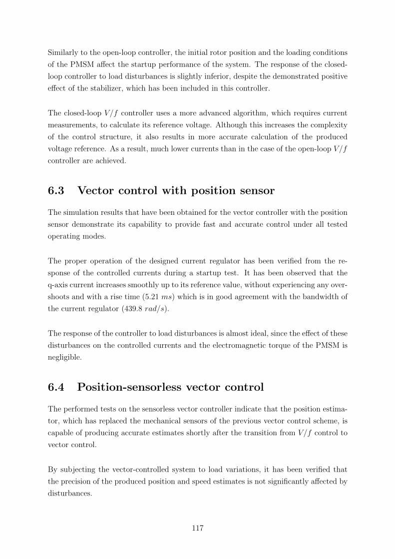
Similarly to the open-loop controller, the initial rotor position and the loading conditions

of the PMSM affect the startup performance of the system. The response of the closed-

loop controller to load disturbances is slightly inferior, despite the demonstrated positive

effect of the stabilizer, which has been included in this controller.

The closed-loop V/f controller uses a more advanced algorithm, which requires current

measurements, to calculate its reference voltage. Although this increases the complexity

of the control structure, it also results in more accurate calculation of the produced

voltage reference. As a result, much lower currents than in the case of the open-loop V/f

controller are achieved.


The simulation results that have been obtained for the vector controller with the position

sensor demonstrate its capability to provide fast and accurate control under all tested

operating modes.

The proper operation of the designed current regulator has been verified from the re-

sponse of the controlled currents during a startup test. It has been observed that the

q-axis current increases smoothly up to its reference value, without experiencing any over-

shoots and with a rise time (5.21 ms) which is in good agreement with the bandwidth of

the current regulator (439.8 rad/s).

The response of the controller to load disturbances is almost ideal, since the effect of these

disturbances on the controlled currents and the electromagnetic torque of the PMSM is

negligible.


The performed tests on the sensorless vector controller indicate that the position estima-

tor, which has replaced the mechanical sensors of the previous vector control scheme, is

capable of producing accurate estimates shortly after the transition from V/f control to

vector control.

By subjecting the vector-controlled system to load variations, it has been verified that

the precision of the produced position and speed estimates is not significantly affected by

disturbances.

117

Both the experimental results and the simulation results show that the effect of load

steps on the current and the electromagnetic torque of the system is insignificant during

vector-controlled operation. This means that the current regulator manages to keep the

controlled quantities close to their target values after load variations.

The efficiency and the torque-producing capability of the vector-controlled system when

the PMSM operates below its rated speed are optimal, because the d-axis current refer-

ence is equal to zero. However, when the field-weakening mode is entered, the efficiency

falls as a result of the commanded demagnetizing current.

For the considered pump load, it has been found that the field-weakening algorithm of

the vector controller can extend the speed range of the PMSM by up to 17.6%. Since the

price that is paid for this extension is a 9.6% decrease in the system efficiency, it would

be sensible to use the field-weakening mode only for short time intervals of high-speed

operation.

The obtained experimental results also demonstrate the capability of the drive to accel-

erate the PMSM by producing a demagnetizing current, while keeping its voltage output

constant. Similarly to the simulations, this results in a significant increase in the total

stator current.

6.5 Future work

Since the focus of this work has been on the development and testing of different control

schemes, the modeling of the considered power system has not been handled in detail.

Due to the simplified representation of the transmission system in the designed models,

phenomena such as the magnetization of the transformers and the charging of the cable

have been neglected in the performed simulations.

In the future, the implemented control schemes can be applied on a more precise model

of the system. The cable connection can be represented with one or more π-equivalent

elements and the magnetizing branch of the transformers can be included in the model.

Furthermore, this thesis has assumed that the voltage at the output of the VSD is si-

nusoidal and equal to the three-phase voltage reference produced by the implemented

controllers. Therefore, the VSD and its output filter have been represented by a simpli-

fied interface between the control circuit and the power circuit.

118

Future work could treat the VSD in a more realistic way. The voltage reference produced

by the implemented controllers should enter a PWM stage, where it should be compared

with a carrier wave. The result of the comparison should determine the form of the volt-

age pulses at the output of the VSD.

Finally, most of the control schemes that have been implemented in this thesis are suitable

for PMSMs with surface-mounted magnets. For PMSMs with significant dq saliency, the

designed models and the developed control algorithms need to be modified. This could

be done in the framework of future research.

119

Bibliography

[1] H. B. Ulvestad, V. Kragset, T. Hollingsæter, S. Alipour, C. Ifrim, H. Allaeddini, and

S. Cheng. Long step start up simulations for high speed permanent magnet motors

in subsea operations. In 15th International IGTE Symposium, page 1, Sept. 2012.

[2] D. Saban and A. Artinian. Permanent-magnet motors for sub-sea applications. Direct

Drive Systems Technical Papers, pages 1–8, 2008.

[3] E. Thibaut, E. Meyer, and P. Bibet. Use of liquid filled motor for subsea pump

applications. In PCIC Europe Conference Record, pages 1–8, June 2010.

[4] J. Flores, J. Burdick, R. Paes, and E. Fidler. Subsea equipment and applications,

a new and emerging technology. In Petroleum and Chemical Industry Conference

Europe, pages 1–8, June 2011.

[5] S. Chi and L. Xu. Development of sensorless vector control for a PMSM running up

to 60,000 rpm. In IEEE International Conference on Electric Machines and Drives,

pages 834–839, May 2005.

[6] S. Ozcira, N. Bekiroglu, and E. Aycicek. Speed control of permanent magnet syn-

chronous motor based on direct torque control method. In International Sympo-

sium on Power Electronics, Electrical Drives, Automation and Motion (SPEEDAM),

pages 268–272, June 2008.

[7] E. Hamdi. Permanent magnet and variable reluctance drive systems. Education and

Training International, Chalmers University of Technology, Goteborg, Sweden, 2003.

[8] K. Chau, C. Chan, and C. Liu. Overview of permanent-magnet brushless drives for

electric and hybrid electric vehicles. IEEE Transactions on Industrial Electronics,

55(6):2246–2257, 2008.

[9] T. Hazel, H. Baerd, J. Bremnes, and J. Legeay. Subsea high-voltage power distribu-

tion. In Petroleum and Chemical Industry Conference, pages 1–9, 2011.

[10] J. Smith, D. Grant, A. Al-Mashgari, and R. Slater. Operation of subsea electrical

submersible pumps supplied over extended length cable systems. IEE Proceedings

on Electric Power Applications, 147(6):544–552, 2000.

120

[11] R. Yacamini, W. Phang, P. Brogan, and A. Scott. Variable speed drives for remote

downhole pump applications. Power Engineering Journal, 14(1):29–36, 2000.

[12] M. Hernes and R. Pittini. Enabling pressure tolerant power electronic converters

for subsea applications. In 13th European Conference on Power Electronics and

Applications, pages 1–10, Sept. 2009.

[13] M. Texiera and J. Houdek. Protecting submersible motors from the effects of PWM

voltage. In Brazil Conference for Quality of Electric Energy (CBQEE), pages 1–6,

2009.

[14] A. Petterteig, R. Pittini, M. Hernes, and Ø. Holt. Pressure tolerant power IGBTs

for subsea applications. In 13th European Conference on Power Electronics and

Applications, pages 1–10, Sept. 2009.

[15] WEG Electrical Equipment, International Division. Induction motors fed by PWM

frequency inverters. Technical guide, 2009.

[16] J. Steinke. Use of an LC filter to achieve a motor-friendly performance of the PWM

voltage source inverter. IEEE Transactions on Energy Conversion, 14(3):649–654,

1999.

[17] ABB Industrial Systems. Effects of AC drives on motor insulation. Technical guide

No. 102, 1998.

[18] P. Finlayson. Output filters for PWM drives with induction motors. In Annual Pulp

and Paper Industry Technical Conference, pages 186–193, June 1997.

[19] K. Haddad. Output filters for PWM drives. General Electrics, Transmission, Dis-

tribution and Industrial Systems, GE Capacitors and Power Quality Products, New

York, USA, 1999.

[20] M. Stulrajter, V. Hrabovcova, and M. Franko. Permanent magnet synchronous

motor control theory. Journal of Electrical Engineering, 58(2):79–84, 2007.

[21] L. Xu and C. Wang. Implementation and experimental investigation of sensorless

control schemes for PMSM in super-high variable speed operation. In Industry Ap-

plications Conference, The 33rd IAS Annual Meeting of the IEEE, pages 483–489,

Oct. 1998.

[22] M. Fatu, R. Teodorescu, I. Boldea, G. Andreescu, and F. Blaabjerg. I-F starting

method with smooth transition to EMF based motion-sensorless vector control of

PM synchronous motor/generator. In IEEE Power Electronics Specialists Conference

(PESC), pages 1481–1487, June 2008.

121

[23] P. Chandana Perera, F. Blaabjerg, J. Pedersen, and P. Thøgersen. A sensorless,

stable V/f control method for permanent-magnet synchronous motor drives. IEEE

Transactions on Industry Applications, 39(3):783–791, 2003.

[24] A. Mishra, J. Makwana, P. Agarwal, and S. Srivastava. Modeling and implementa-

tion of vector control for PM synchronous motor drive. In International Conference

on Advances in Engineering, Science and Management (ICAESM), pages 582–585,

Mar. 2012.

[25] N. Ertugrul and P. Acarnley. A new algorithm for sensorless operation of permanent

magnet motors. IEEE Transactions on Industry Applications, 30(1):126–133, 1994.

[26] P. Chandana Perera. Sensorless control of permanent-magnet synchronous motor

drives. Ph.D thesis, Aalborg University, Institute of Energy Technology, Aalborg,

Denmark, Feb. 2002.

[27] P. Acarnley and J. Watson. Review of position-sensorless operation of brush-

less permanent-magnet machines. IEEE Transactions on Industrial Electronics,

53(2):352–362, 2006.

[28] C. French and P. Acarnley. Control of permanent magnet motor drives using a

new position estimation technique. IEEE Transactions on Industry Applications,

32(5):1089–1097, 1996.

[29] S. Ostlund and M. Brokemper. Permanent magnet synchronous motor control theory.

IEEE Transactions on Industry Applications, 32(5):1158–1165, 1996.

[30] J. Xuewu and L. Yingchao. Field weakening control of PMSM used in an electric

power steering system. In International Conference on Electric Information and

Control Engineering (ICEICE), pages 2194–2199, Apr. 2011.

[31] M. Zordan, P. Vas, M. Rashed, S. Bolognani, and M. Zigliotto. Field-weakening

in vector controlled and DTC PMSM drives, a comparative analysis. In Eighth In-

ternational Conference on Power Electronics and Variable Speed Drives (IEE Conf.

Publ. No. 475), pages 493–499, Sept. 2000.

[32] H. Mahmoudi and A. Lagrioui. Flux-weakening control of permanent magnet syn-

chronous machines. Journal of Theoretical and Applied Information Technology,

34(2):110–117, 2011.

[33] R. Dolecek, J. Novak, and O. Cerny. Traction permanent magnet synchronous motor

torque control with flux weakening. Radioengineering, 18(4):601–605, 2009.

122

[34] V. Jevremovic and D. Marcetic. A simple closed-loop flux-weakening for permanent

magnet synchronous motors. In 14th International Symposium on Power Electronics,

pages 1–4, Nov. 2007.

[35] L. Harnefors. Control of variable-speed drives. Applied Signal Processing and Con-

trol, Department of Electronics, Malardalen University, Vasteras, Sweden, 2002.

[36] J. Pyrhonen. Electrical drives. Department of Electrical Engineering, Lappeenranta

University of Technology, Lappeenranta, Finland, 2009.

[37] H. Saadat. Power System Analysis. McGraw-Hill Series in Electrical and Computer

Engineering, 1999.

[38] N. Mohan, T. Undeland, and W. Robbins. Power Electronics: Converters, Applica-

tions, and Design. John Wiley and Sons Inc., 1995.

[39] R. Krishnan. Control and operation of PM synchronous motor drives in the field-

weakening region. In Proceedings of the IECON ’93., International Conference on

Industrial Electronics, Control, and Instrumentation, pages 745–750, Nov. 1993.

[40] P. Fajkus, B. Klima, and P. Hutak. High speed range field oriented control for perma-

nent magnet synchronous motor. In International Symposium on Power Electronics,

Electrical Drives, Automation and Motion (SPEEDAM), pages 225–230, June 2012.

123

Documents

SensorlessscalarandvectorcontrolofasubseaPMSMpublications.lib.chalmers.se/records/fulltext/183931/183931.pdf · Master s Thesis 2005:22. ... This thesis deals with the position-sensorless