Embed Size (px)
Citation preview
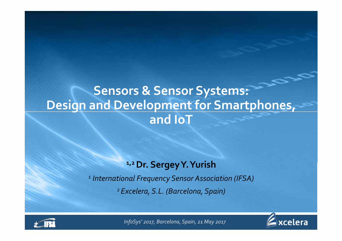
Sensors & Sensor Systems: Design and Development for Smartphones,
and IoT
1,2 Dr. Sergey Y. Yurish1 International Frequency Sensor Association (IFSA)
2 Excelera, S.L. (Barcelona, Spain)
InfoSys’ 2017, Barcelona, Spain, 21 May 2017
Contents
Introduction
Sensor types and classification
Advanced Design Approach
Examples
From “Smart” to “Intelligent”
Summary
Contents
Introduction
Sensor types and classification
Advanced Design Approach
Examples
From “Smart” to “Intelligent”
Summary
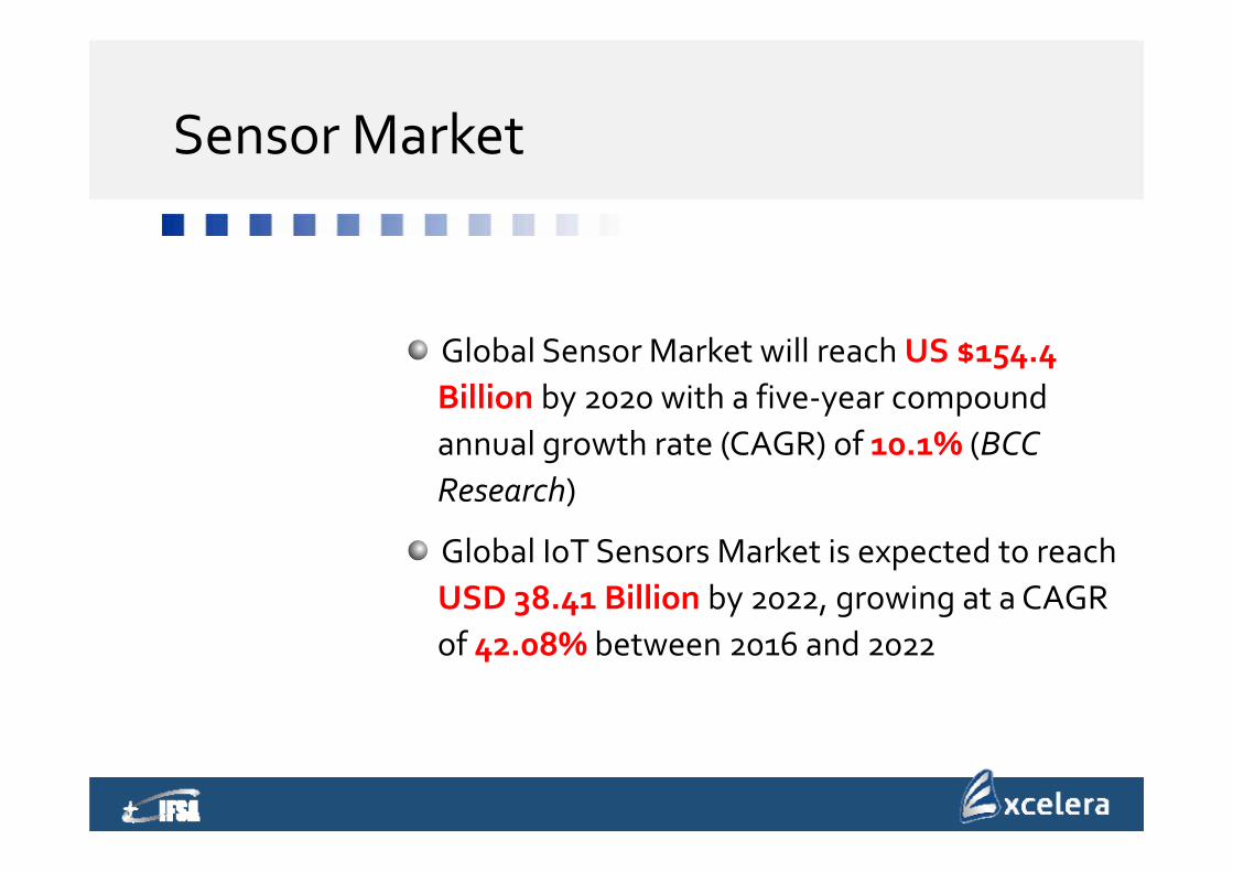
Sensor Market
Global Sensor Market will reach US $154.4 Billion by 2020 with a five‐year compound annual growth rate (CAGR) of 10.1% (BCC Research)
Global IoT Sensors Market is expected to reach USD 38.41 Billion by 2022, growing at a CAGR of 42.08% between 2016 and 2022
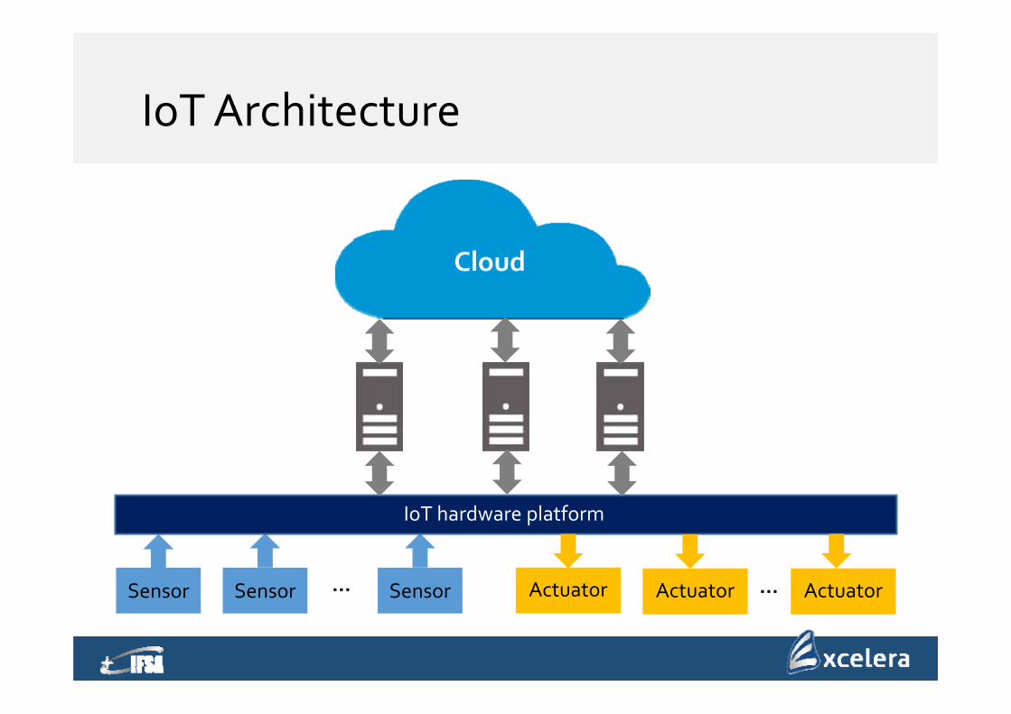
IoTArchitecture
Sensor SensorSensor Actuator Actuator Actuator… …
IoT hardware platform
Cloud
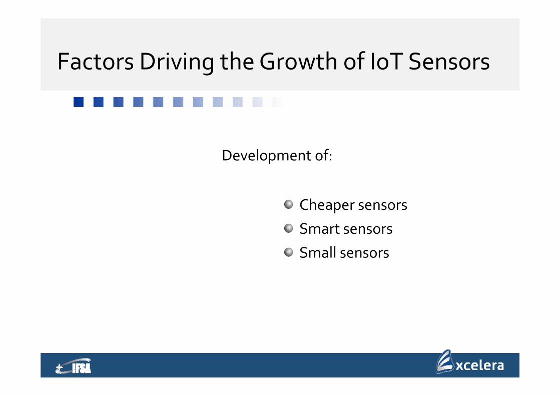
Factors Driving the Growth of IoT Sensors
Cheaper sensors
Smart sensors
Small sensors
Development of:
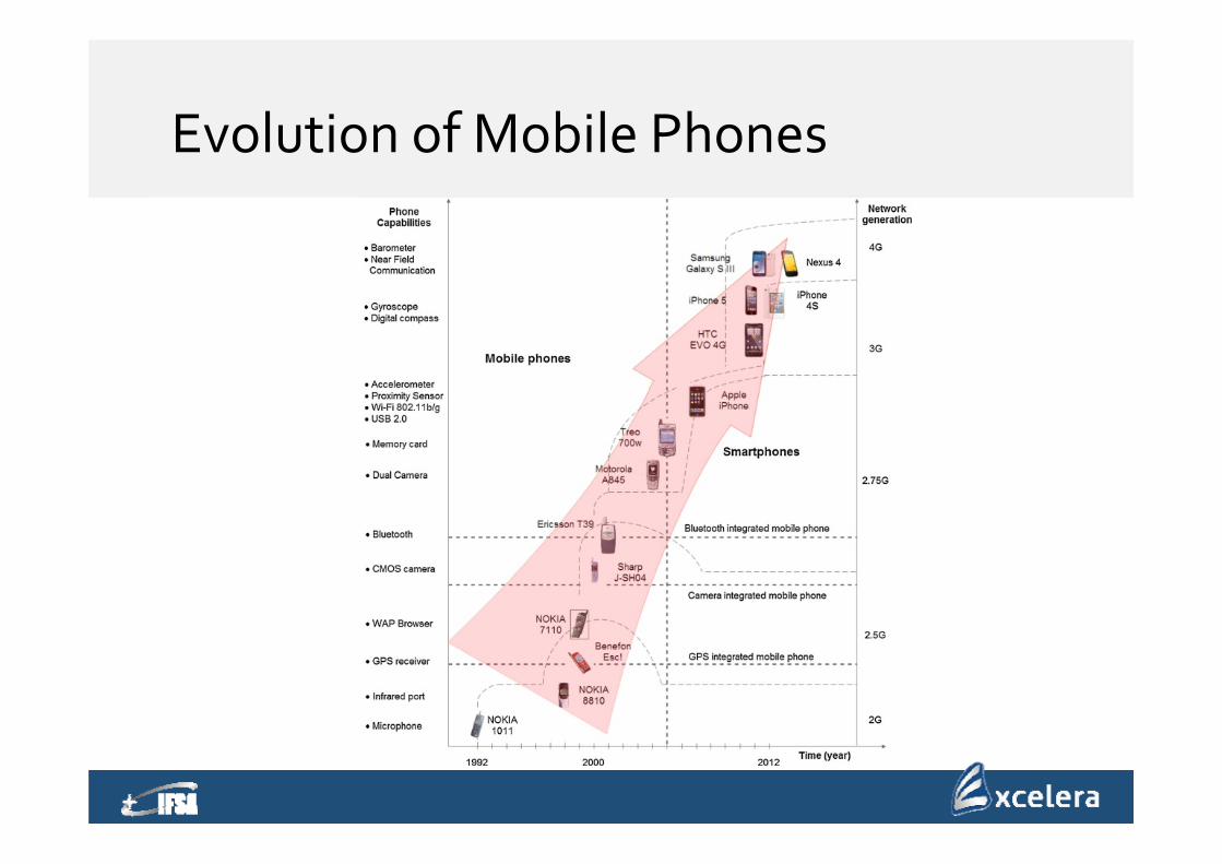
Evolution of Mobile Phones
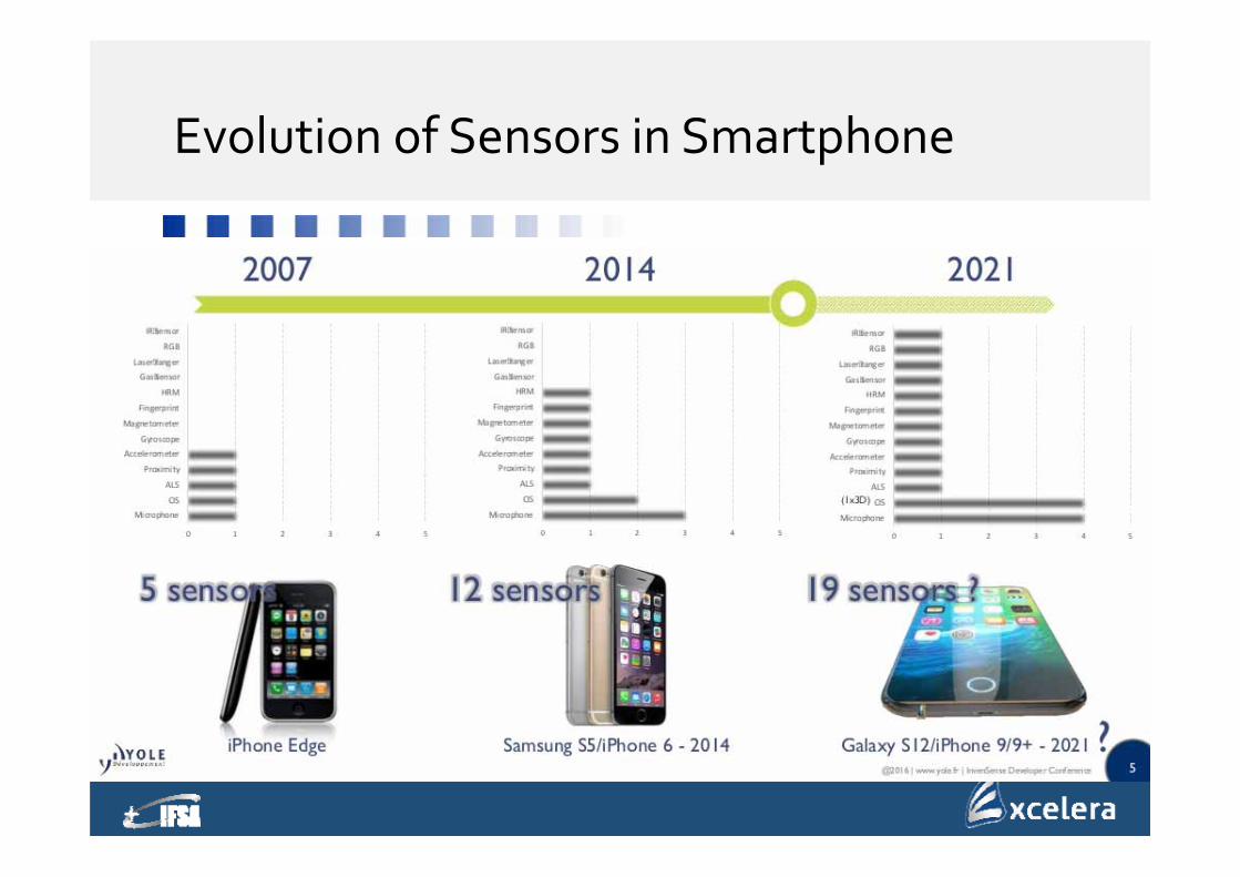
Evolution of Sensors in Smartphone
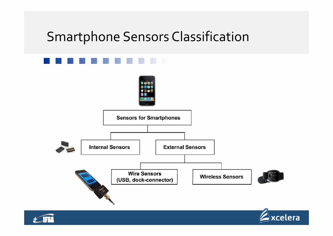
Smartphone Sensors Classification
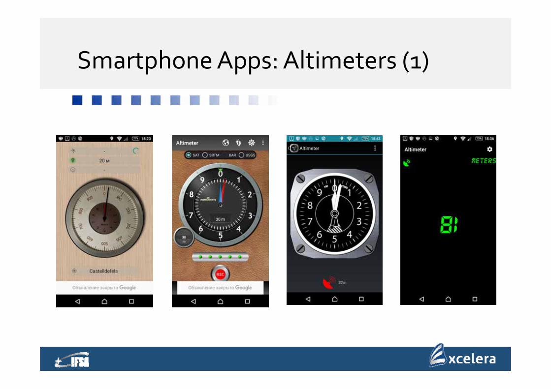
Smartphone Apps: Altimeters (1)
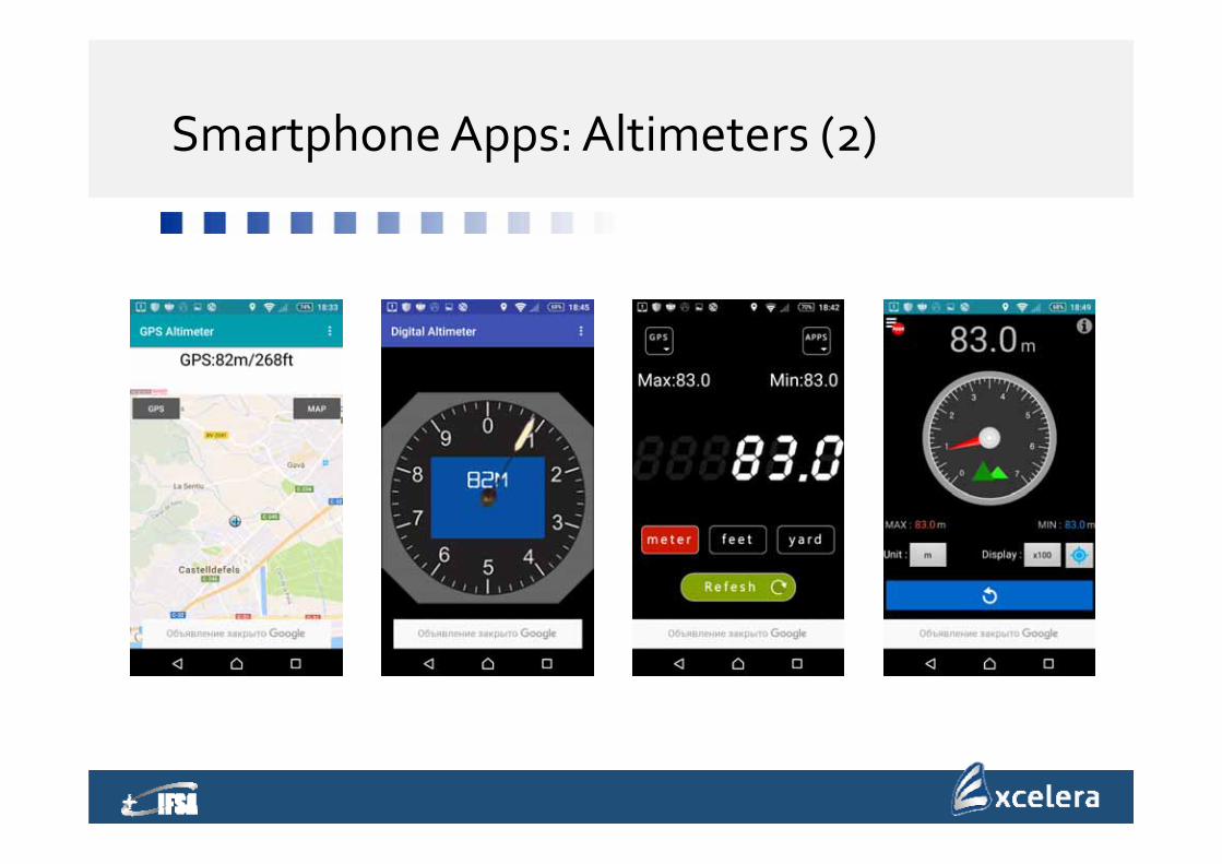
Smartphone Apps: Altimeters (2)
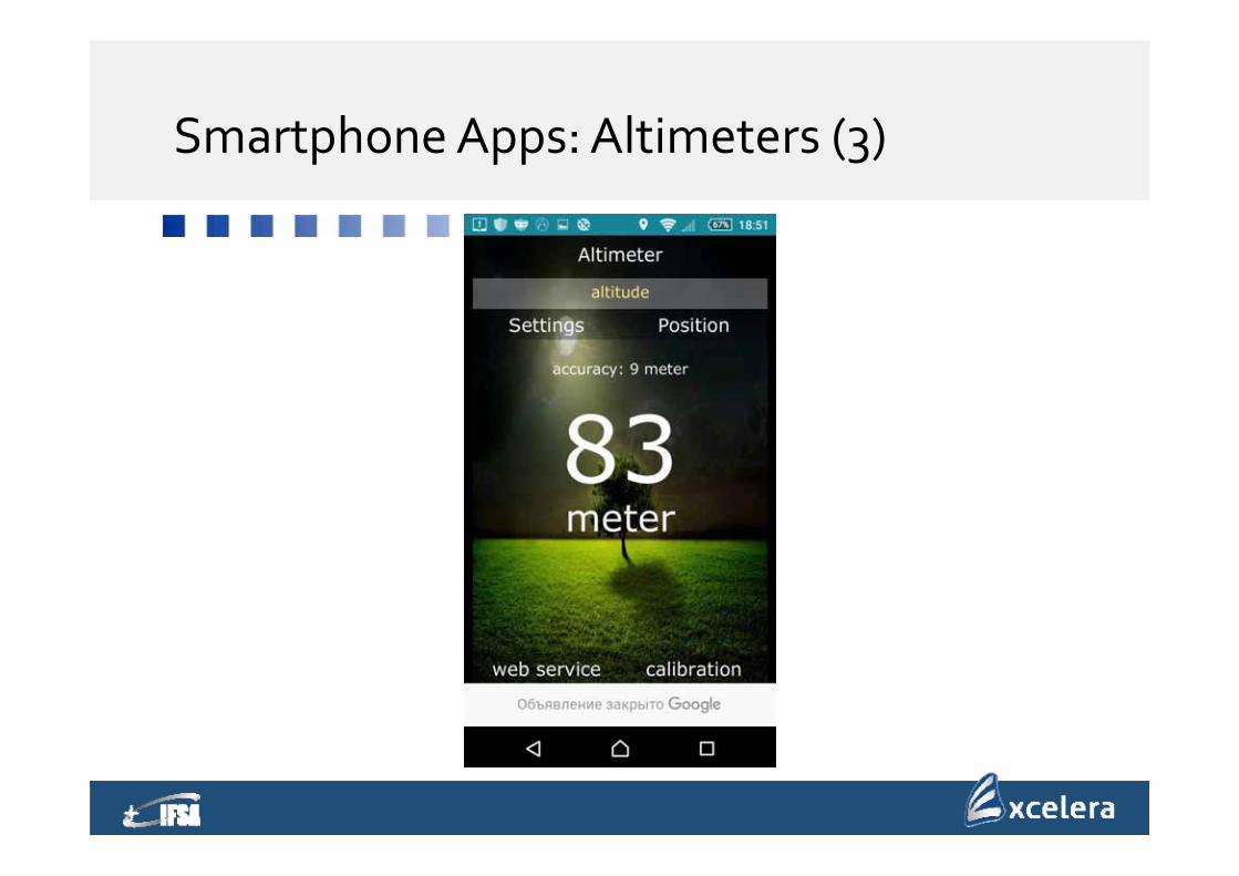
Smartphone Apps: Altimeters (3)
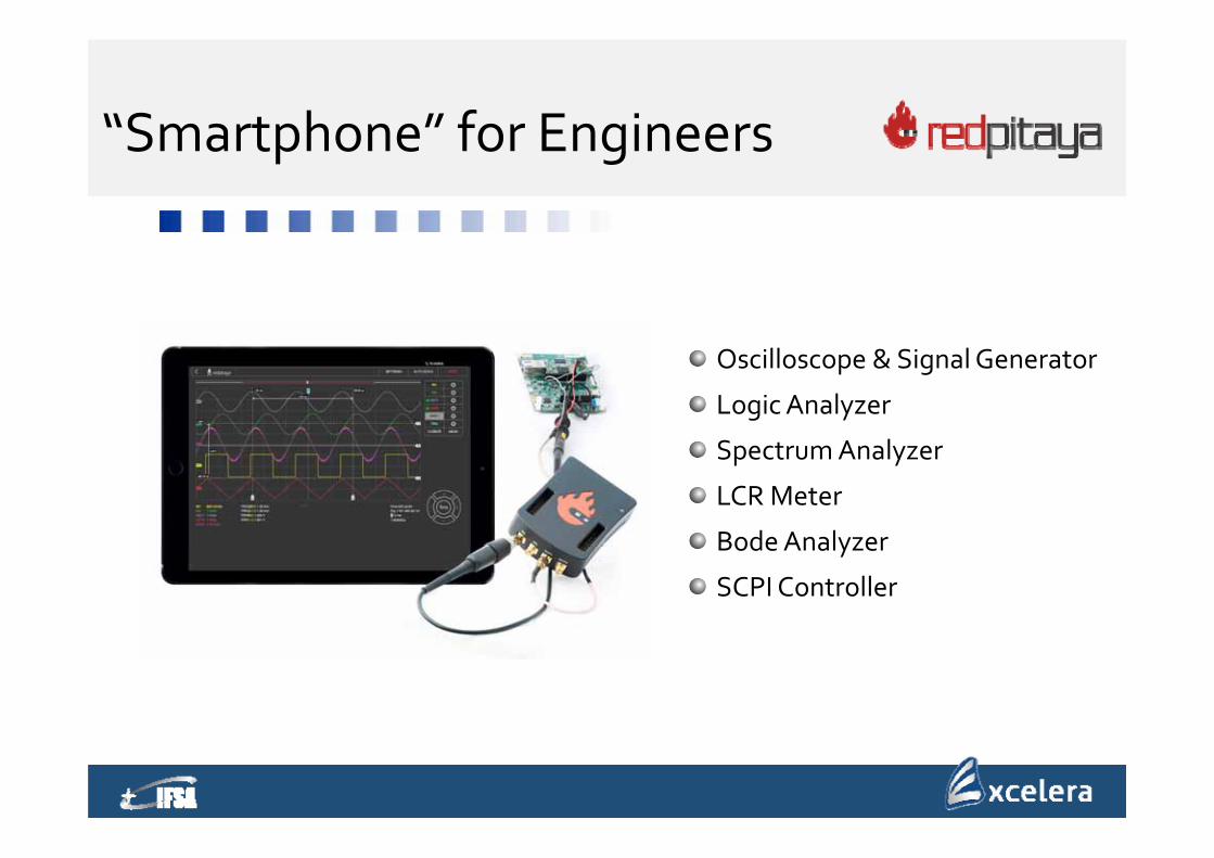
“Smartphone” for Engineers
Oscilloscope & Signal Generator
Logic Analyzer
Spectrum Analyzer
LCR Meter
Bode Analyzer
SCPI Controller
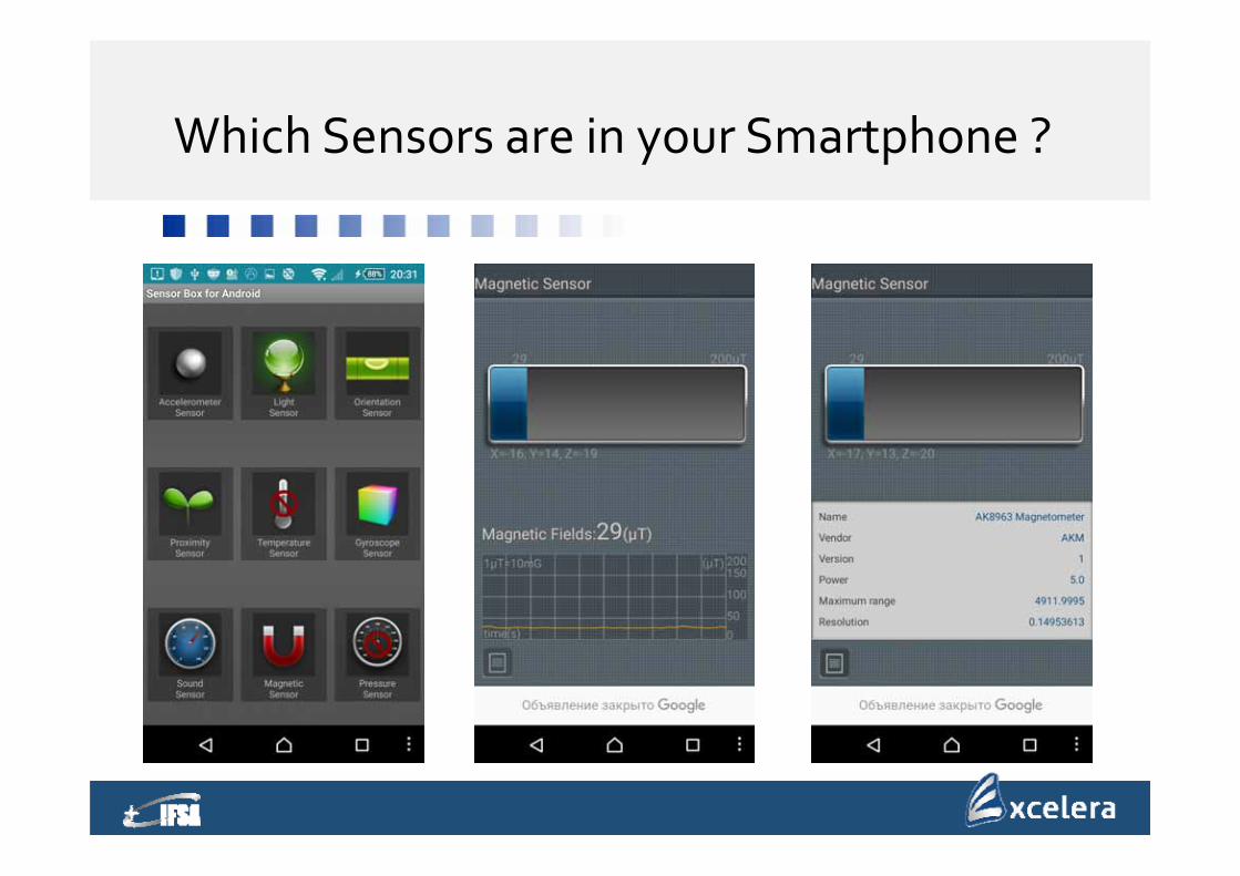
Which Sensors are in your Smartphone ?

Agenda
Introduction
Sensor types and classification
Advanced Design Approach
Examples
From “Smart” to “Intelligent”
Summary
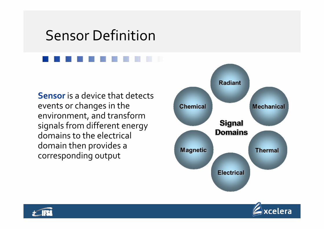
Sensor Definition
Sensor is a device that detects events or changes in the environment, and transform signals from different energy domains to the electrical domain then provides a corresponding output
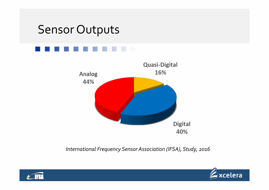
Sensor Outputs
International Frequency Sensor Association (IFSA), Study, 2016
Analog & Quasi‐Digital Sensors
Analog sensor ‐ sensor based on the usage of anamplitude modulation of electromagnetic processes
Quasi‐digital sensors are discrete frequency‐timedomain sensors with frequency, period, duty‐cycle, timeinterval, pulse number or phase shift output
Quasi‐digital sensors combine a simplicity anduniversatility that is inherent to analog devices andaccuracy and noise immunity, proper to sensors withdigital output
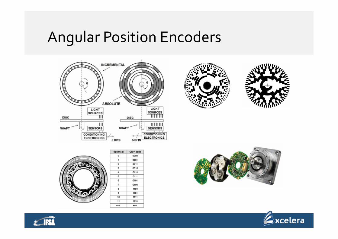
Angular Position Encoders
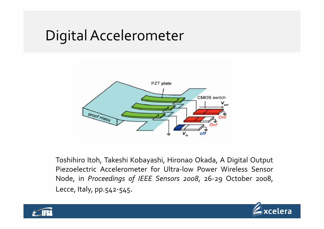
Digital Accelerometer
Toshihiro Itoh, Takeshi Kobayashi, Hironao Okada, A Digital OutputPiezoelectric Accelerometer for Ultra‐low Power Wireless SensorNode, in Proceedings of IEEE Sensors 2008, 26‐29 October 2008,Lecce, Italy, pp.542‐545.
Digital Sensors
Number of physical phenomenon, on the basis of which direct conversion sensors with digital outputs can be designed, is essentially limited
Angular‐position encoders and cantilever‐based accelerometers –examples of digital sensors of direct conversion
There are not any nature phenomenon with discrete performances changing under pressure, temperature, etc.
Technological Limitations
Below the 100 nm technology processes the design of analog and mixed‐signal circuits becomes essentially more difficult
Long development time, risk, cost, low yield rate and the need for very high volumes
The limitation is not only an increased design effort but also a growing power consumption
However, digital circuits becomes faster, smaller, and less power hungry
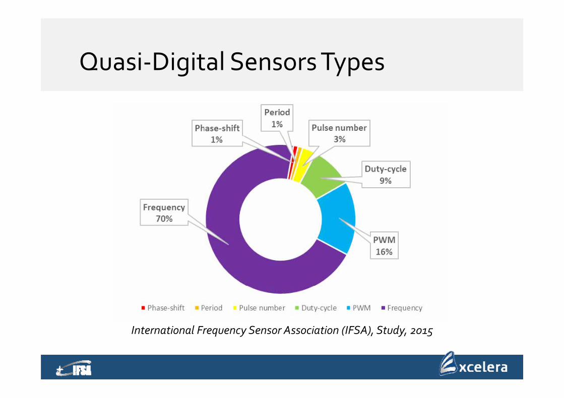
Quasi‐Digital Sensors Types
International Frequency Sensor Association (IFSA), Study, 2015
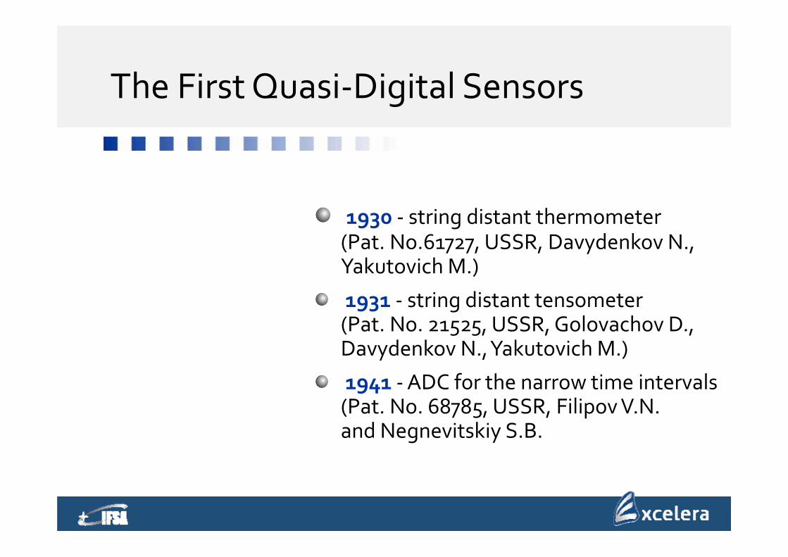
The First Quasi‐Digital Sensors
1930 ‐ string distant thermometer (Pat. No.61727, USSR, Davydenkov N., YakutovichM.)
1931 ‐ string distant tensometer(Pat. No. 21525, USSR, Golovachov D., Davydenkov N., YakutovichM.)
1941 ‐ADC for the narrow time intervals (Pat. No. 68785, USSR, FilipovV.N. and Negnevitskiy S.B.
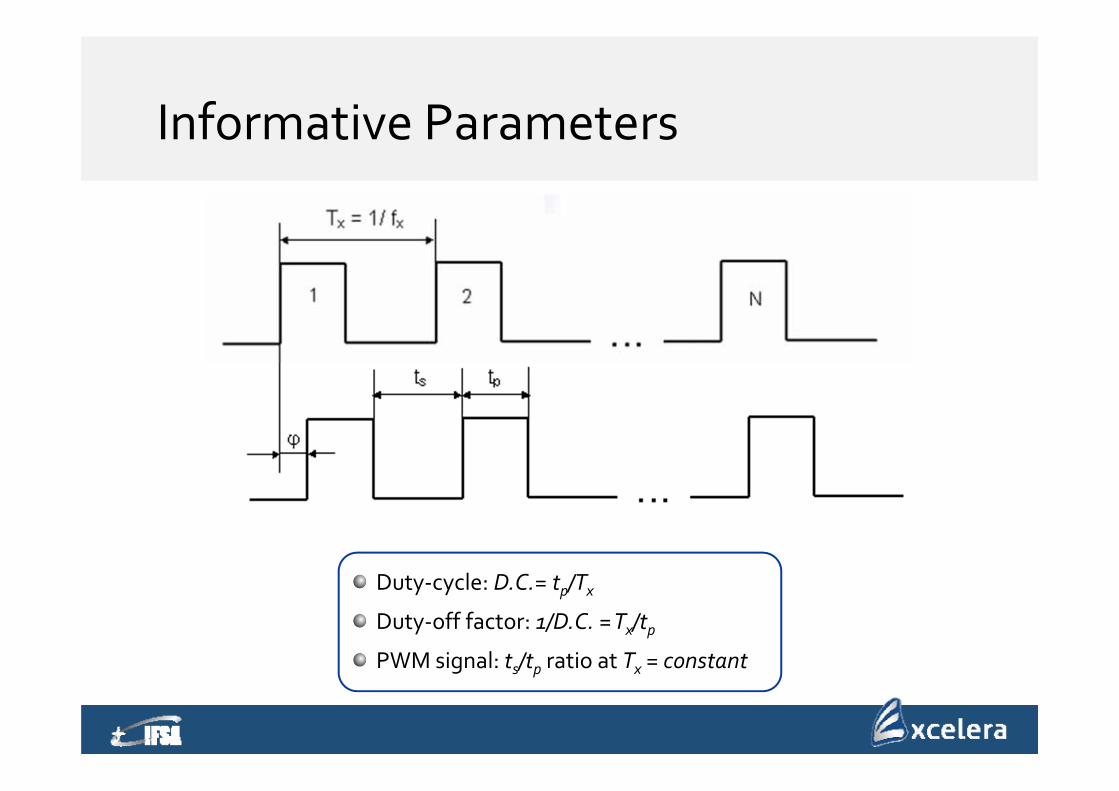
Informative Parameters
Duty‐cycle: D.C.= tp/TxDuty‐off factor: 1/D.C. = Tx/tpPWM signal: ts/tp ratio at Tx = constant
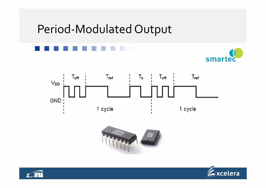
Period‐Modulated Output
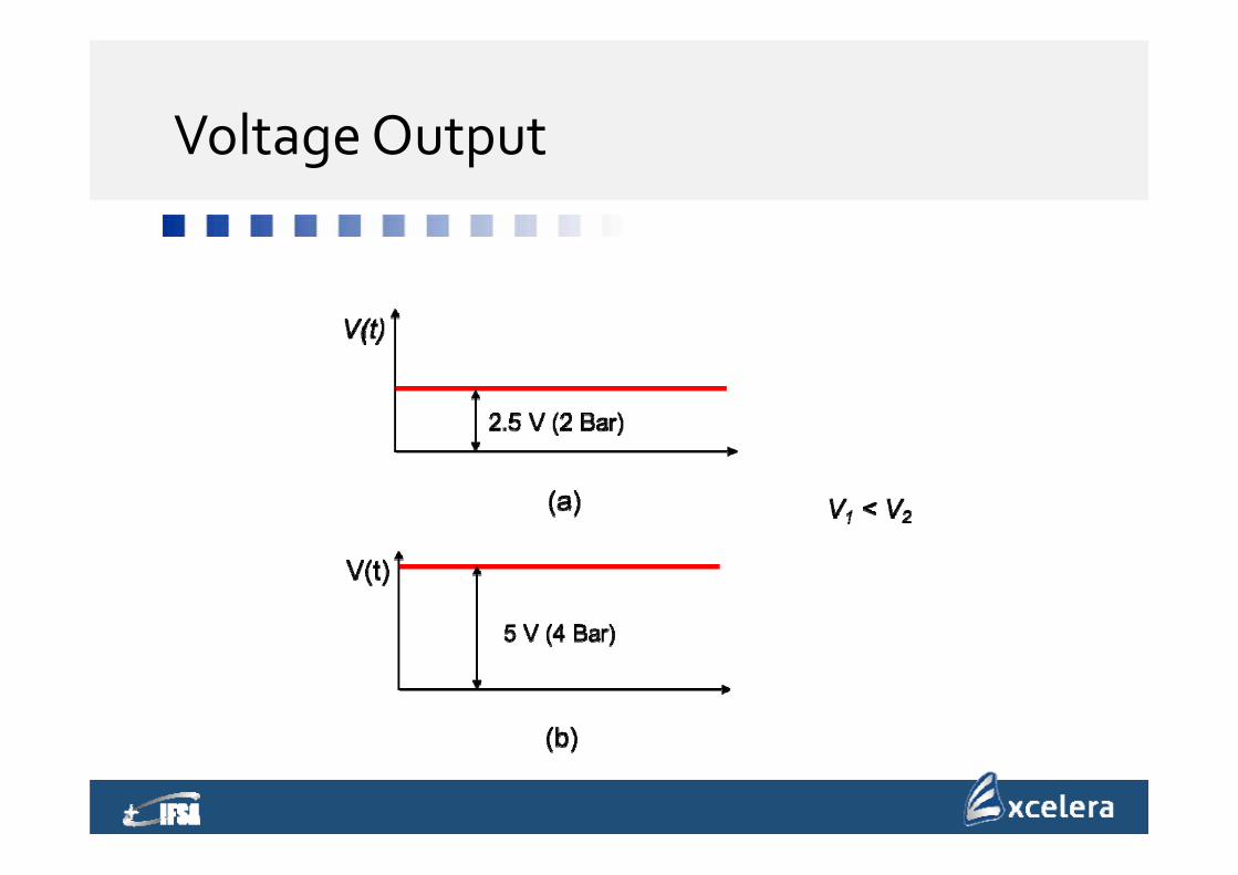
Voltage Output
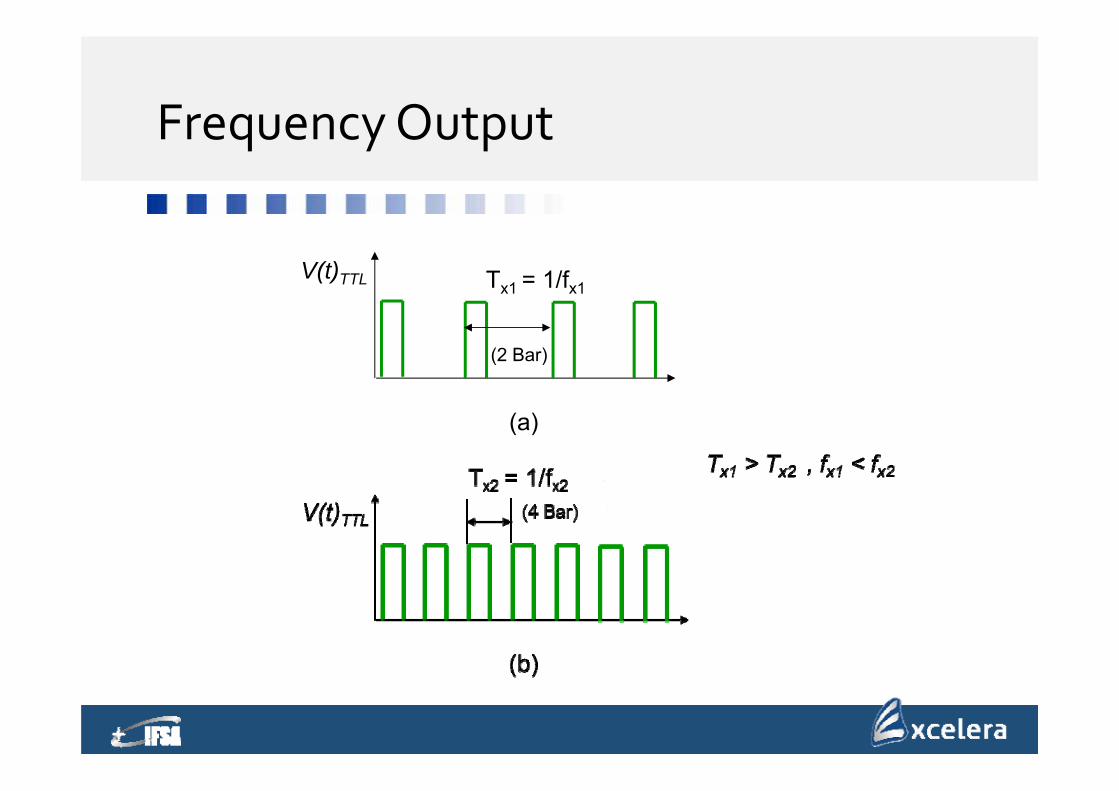
Frequency Output
(a)
V(t)TTL Tx1 = 1/fx1
(2 Bar)
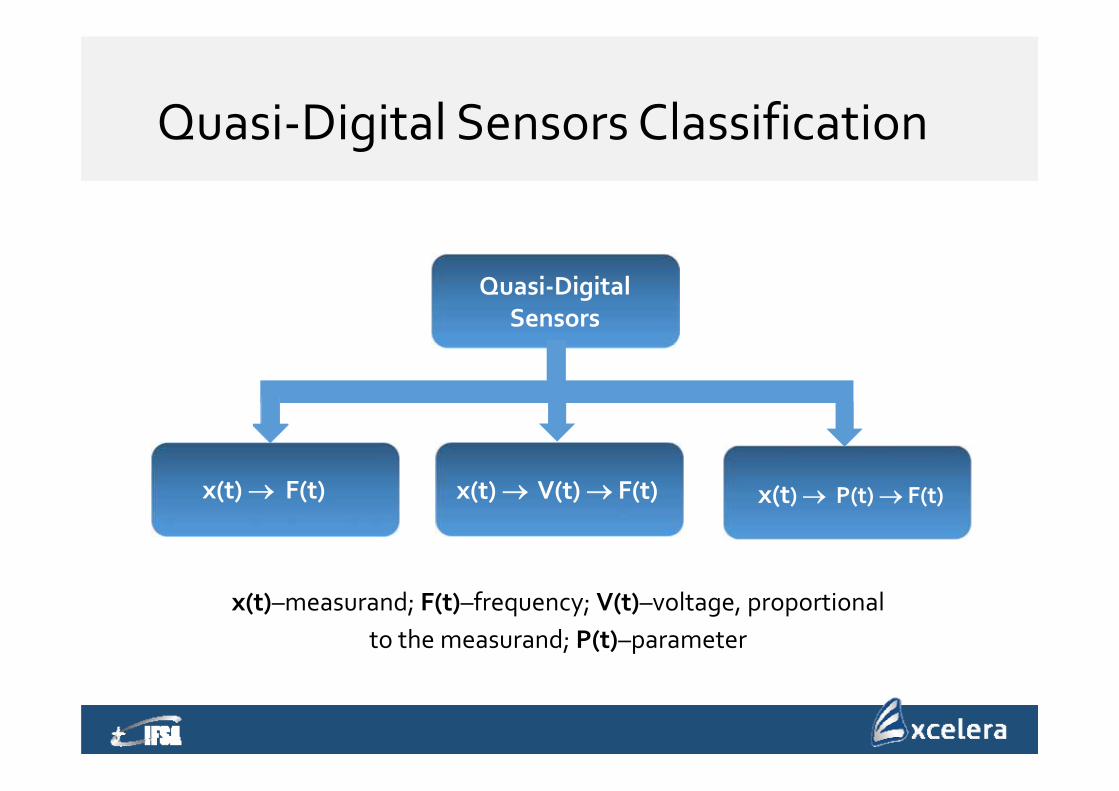
Quasi‐Digital Sensors Classification
x(t)–measurand; F(t)–frequency; V(t)–voltage, proportional to the measurand; P(t)–parameter
Quasi‐DigitalSensors
x(t) F(t) x(t) V(t) F(t) x(t) P(t) F(t)
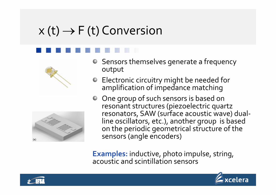
x (t) F (t) Conversion
Sensors themselves generate a frequency outputElectronic circuitry might be needed for amplification of impedance matchingOne group of such sensors is based on resonant structures (piezoelectric quartz resonators, SAW (surface acoustic wave) dual‐line oscillators, etc.), another group is based on the periodic geometrical structure of the sensors (angle encoders)
Examples: inductive, photo impulse, string, acoustic and scintillation sensors
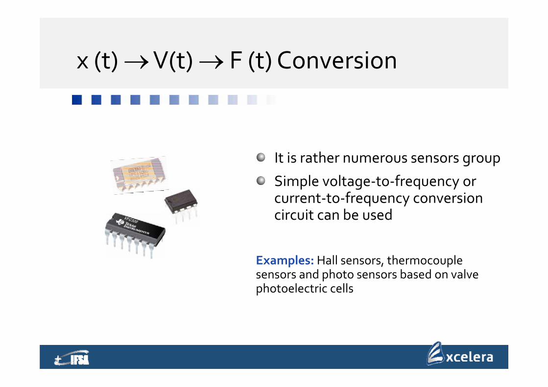
x (t) V(t) F (t) Conversion
It is rather numerous sensors group
Simple voltage‐to‐frequency or current‐to‐frequency conversion circuit can be used
Examples:Hall sensors, thermocouple sensors and photo sensors based on valve photoelectric cells
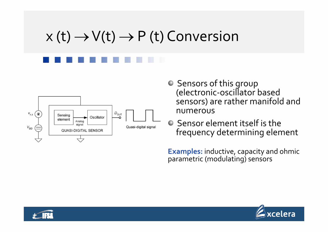
x (t) V(t) P (t) Conversion
Sensors of this group (electronic‐oscillator based sensors) are rather manifold and numerousSensor element itself is the frequency determining element
Examples: inductive, capacity and ohmicparametric (modulating) sensors
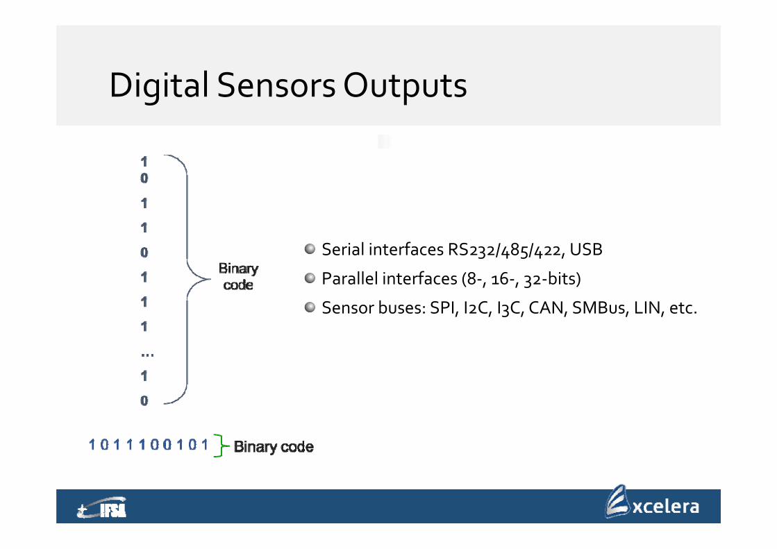
Digital Sensors Outputs
Serial interfaces RS232/485/422, USB
Parallel interfaces (8‐, 16‐, 32‐bits)
Sensor buses: SPI, I2C, I3C, CAN, SMBus, LIN, etc.
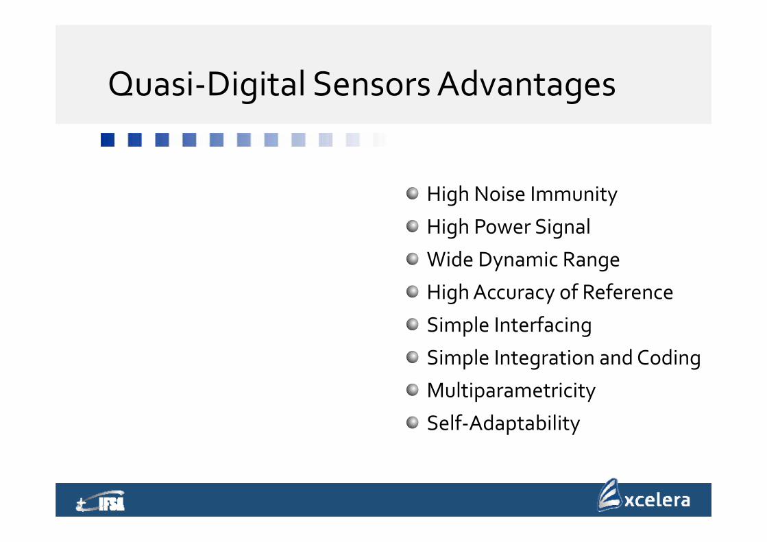
Quasi‐Digital Sensors Advantages
High Noise Immunity
High Power Signal
Wide Dynamic Range
High Accuracy of Reference
Simple Interfacing
Simple Integration and Coding
Multiparametricity
Self‐Adaptability
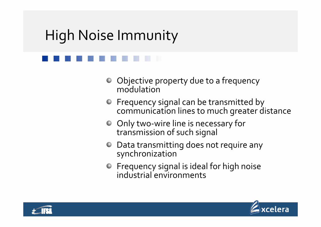
High Noise Immunity
Objective property due to a frequency modulationFrequency signal can be transmitted by communication lines to much greater distanceOnly two‐wire line is necessary for transmission of such signalData transmitting does not require any synchronizationFrequency signal is ideal for high noise industrial environments
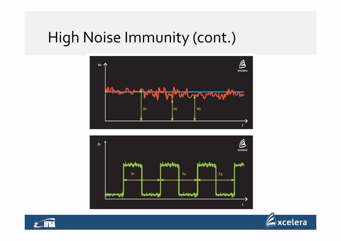
High Noise Immunity (cont.)
High Power Signal
Section from a sensor output up to an amplifier input is the heaviest section in a measuring channel for signal transmitting from a power point of viewLosses, originating on this section can not be filled any more by any signal processingOutput powers of frequency sensors, as a rule, are considerably higher
Wide Dynamic Range
Dynamic range is not limited by supply voltage and noise
Dynamic range of over 160 dB can be easily obtained

High Accuracy of Reference
Crystal oscillators can be made more stable, than the voltage reference:
‐ non‐compensated crystal oscillator has up to (150)∙10‐6 error
‐ temperature‐compensated crystal oscillator has up to 10‐8 10‐10 error
Minimum possible error for frequency measurements with the help of quantum frequency standard is 10‐14, minimum possible quantization step for time interval is 10‐12 seconds
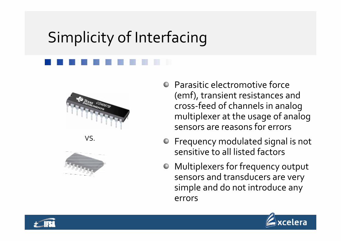
Simplicity of Interfacing
Parasitic electromotive force (emf), transient resistances and cross‐feed of channels in analogmultiplexer at the usage of analogsensors are reasons for errors
Frequency modulated signal is not sensitive to all listed factors
Multiplexers for frequency output sensors and transducers are very simple and do not introduce any errors
VS.
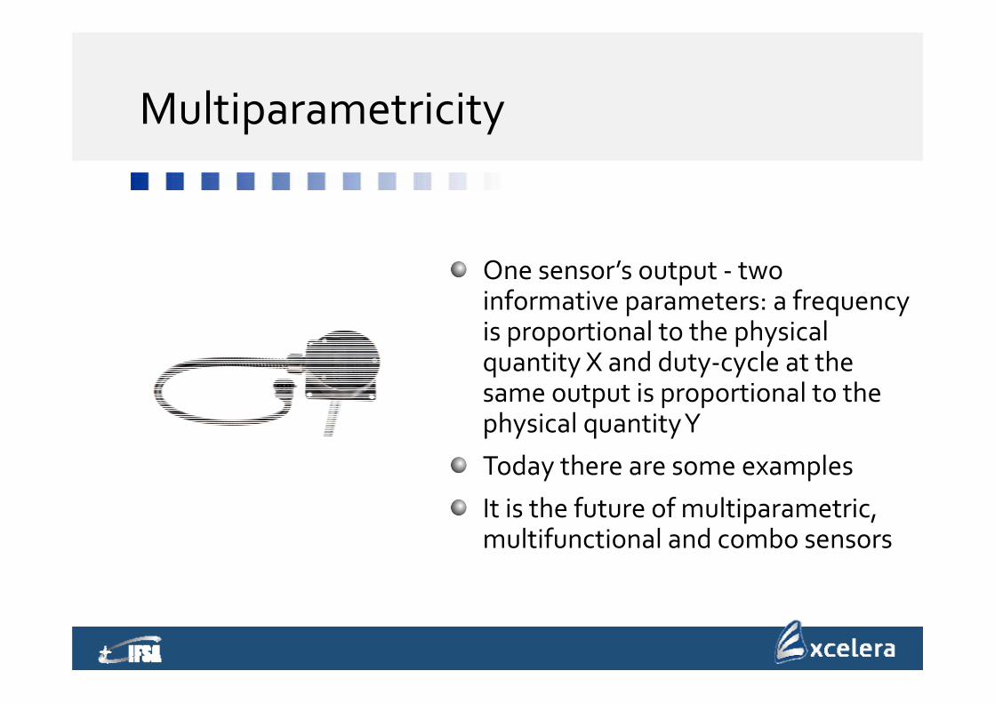
Multiparametricity
One sensor’s output ‐ two informative parameters: a frequency is proportional to the physical quantity X and duty‐cycle at the same output is proportional to the physical quantity Y
Today there are some examples
It is the future of multiparametric, multifunctional and combo sensors
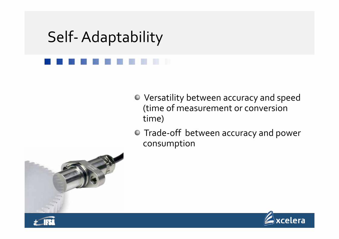
Self‐Adaptability
Versatility between accuracy and speed (time of measurement or conversion time)
Trade‐off between accuracy and power consumption
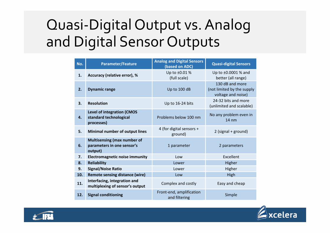
Quasi‐Digital Output vs. Analog and Digital Sensor Outputs
No. Parameter/Feature Analog and Digital Sensors (based on ADC) Quasi‐digital Sensors
1. Accuracy (relative error), % Up to ±0.01 % (full scale)
Up to ±0.0001 % and better (all range)
2. Dynamic range Up to 100 dB 130 dB and more
(not limited by the supply voltage and noise)
3. Resolution Up to 16‐24 bits 24‐32 bits and more (unlimited and scalable)
4. Level of integration (CMOS standard technological processes)
Problems below 100 nm No any problem even in 14 nm
5. Minimal number of output lines 4 (for digital sensors + ground) 2 (signal + ground)
6. Multisensing (max number of parameters in one sensor’s output)
1 parameter 2 parameters
7. Electromagnetic noise immunity Low Excellent8. Reliability Lower Higher9. Signal/Noise Ratio Lower Higher10. Remote sensing distance (wire) Low High
11. Interfacing, integration and multiplexing of sensor’s output Complex and costly Easy and cheap
12. Signal conditioning Front‐end, amplification and filtering Simple
Quasi‐Digital Sensors on SWP
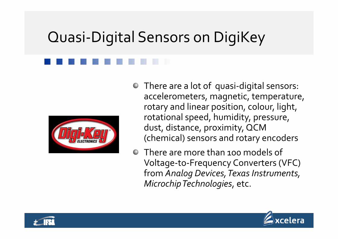
Quasi‐Digital Sensors on DigiKey
There are a lot of quasi‐digital sensors: accelerometers, magnetic, temperature, rotary and linear position, colour, light, rotational speed, humidity, pressure, dust, distance, proximity, QCM (chemical) sensors and rotary encoders
There are more than 100 models of Voltage‐to‐Frequency Converters (VFC) from Analog Devices, Texas Instruments, Microchip Technologies, etc.
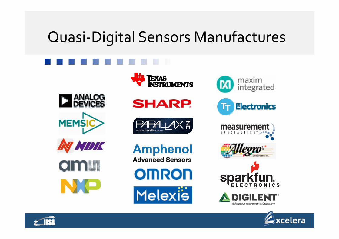
Quasi‐Digital Sensors Manufactures
Quasi‐Digital Sensors: Summary
There are many quasi‐digital sensors and transducers for any physical and chemical, electrical and non electrical quantitiesVarious frequency‐time parameters of signals are used as informative parameters: fx, Tx, D.C., PWM, T, x, etc.The frequency range is very broad: from some parts of Hz to some MHzRelative error up to ±0.01% and better
Agenda
Introduction
Sensor types and classification
Advanced Design Approach
Examples
From “Smart” to “Intelligent”
Summary
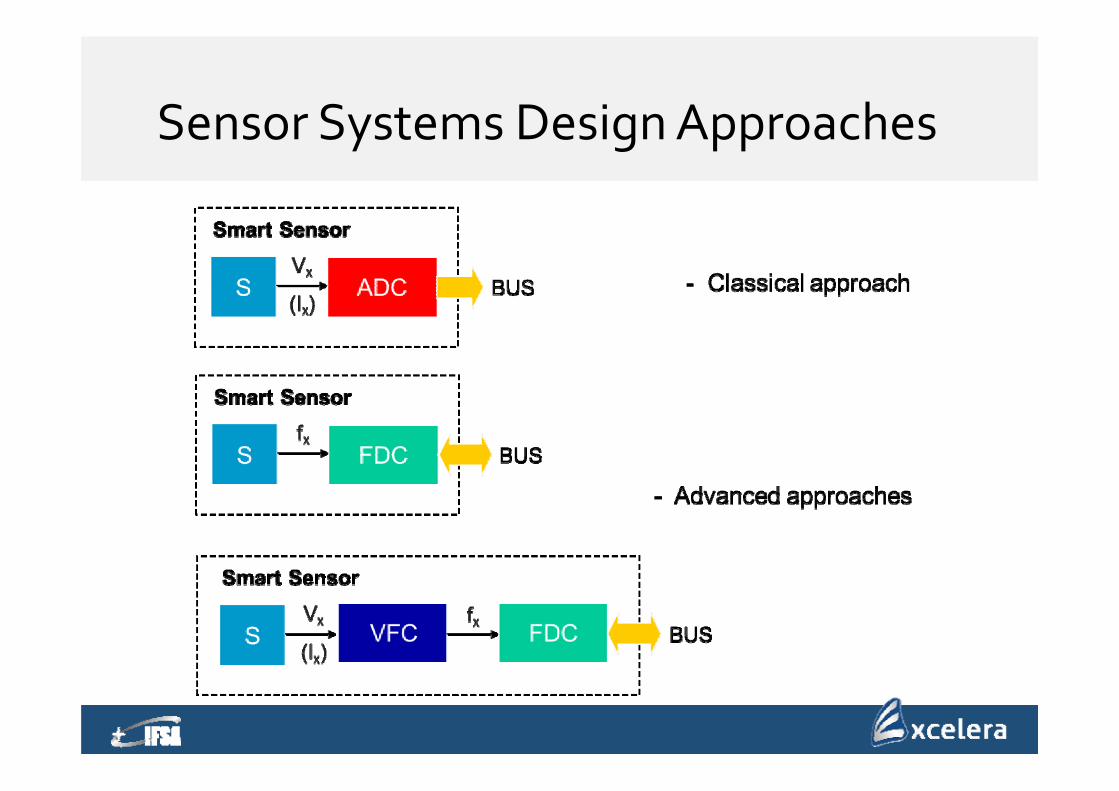
Sensor Systems Design Approaches
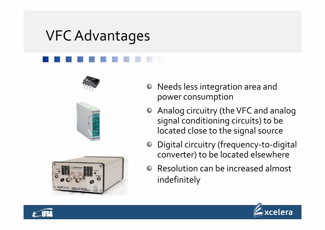
VFCAdvantages
Needs less integration area and power consumption
Analog circuitry (the VFC and analog signal conditioning circuits) to be located close to the signal source
Digital circuitry (frequency‐to‐digital converter) to be located elsewhere
Resolution can be increased almost indefinitely
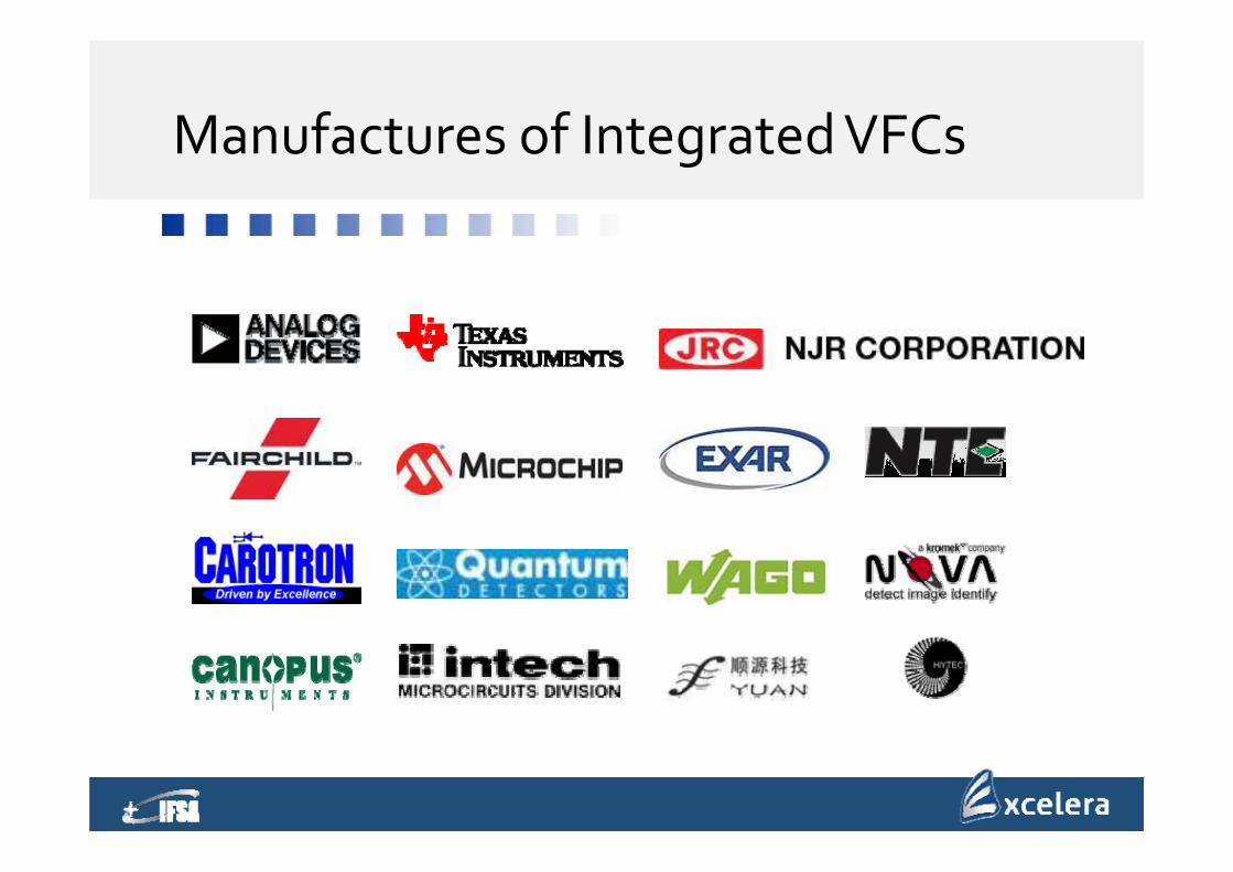
Manufactures of Integrated VFCs
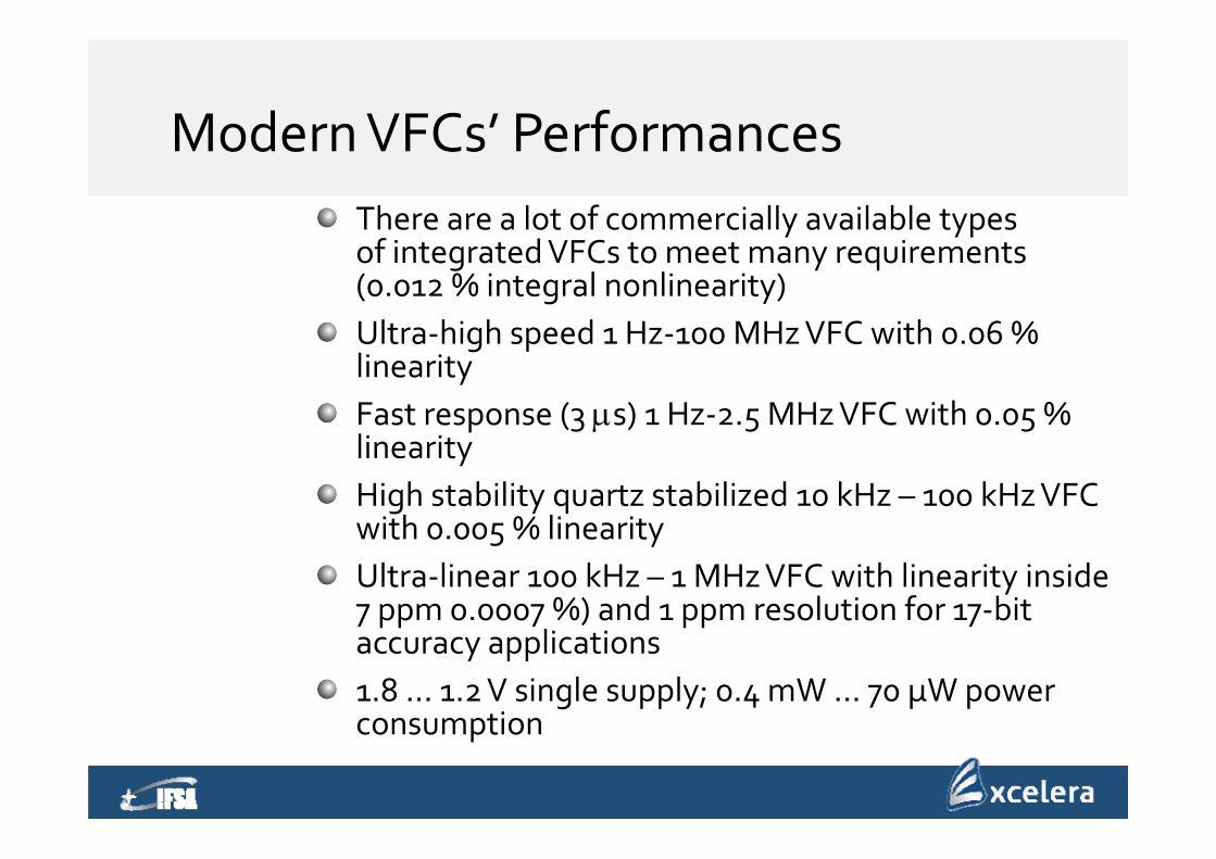
Modern VFCs’ PerformancesThere are a lot of commercially available types of integrated VFCs to meet many requirements (0.012 % integral nonlinearity)Ultra‐high speed 1 Hz‐100 MHz VFC with 0.06 % linearityFast response (3 s) 1 Hz‐2.5 MHz VFC with 0.05 % linearityHigh stability quartz stabilized 10 kHz – 100 kHz VFC with 0.005 % linearityUltra‐linear 100 kHz – 1 MHz VFC with linearity inside 7 ppm 0.0007 %) and 1 ppm resolution for 17‐bit accuracy applications1.8 … 1.2 V single supply; 0.4 mW… 70 µW power consumption
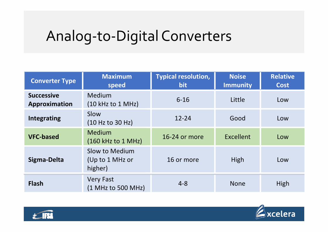
Analog‐to‐Digital Converters
Converter Type Maximumspeed
Typical resolution, bit
Noise Immunity
Relative Cost
Successive Approximation
Medium(10 kHz to 1 MHz) 6‐16 Little Low
Integrating Slow(10 Hz to 30 Hz) 12‐24 Good Low
VFC‐based Medium(160 kHz to 1 MHz) 16‐24 or more Excellent Low
Sigma‐Delta Slow to Medium (Up to 1 MHz or higher)
16 or more High Low
Flash Very Fast(1 MHz to 500 MHz) 4‐8 None High
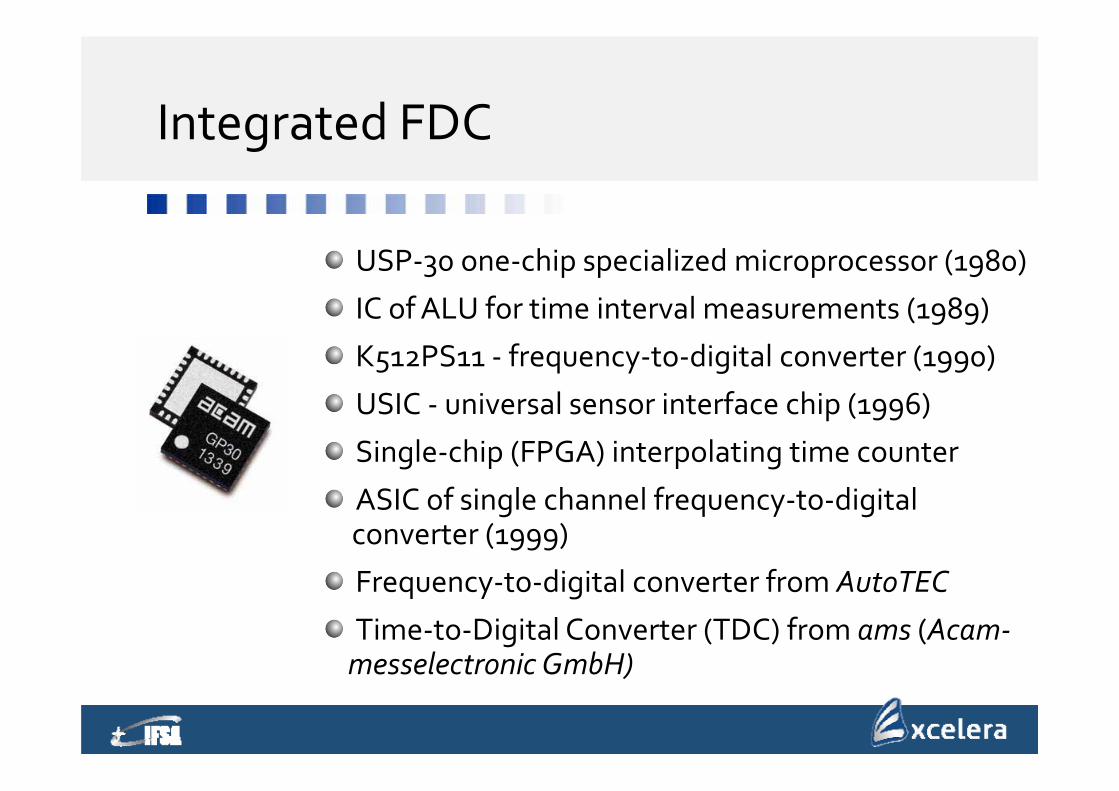
Integrated FDC
USP‐30 one‐chip specialized microprocessor (1980)
IC of ALU for time interval measurements (1989)
K512PS11 ‐ frequency‐to‐digital converter (1990)
USIC ‐ universal sensor interface chip (1996)
Single‐chip (FPGA) interpolating time counter
ASIC of single channel frequency‐to‐digital converter (1999)
Frequency‐to‐digital converter from AutoTEC
Time‐to‐Digital Converter (TDC) from ams (Acam‐messelectronic GmbH)
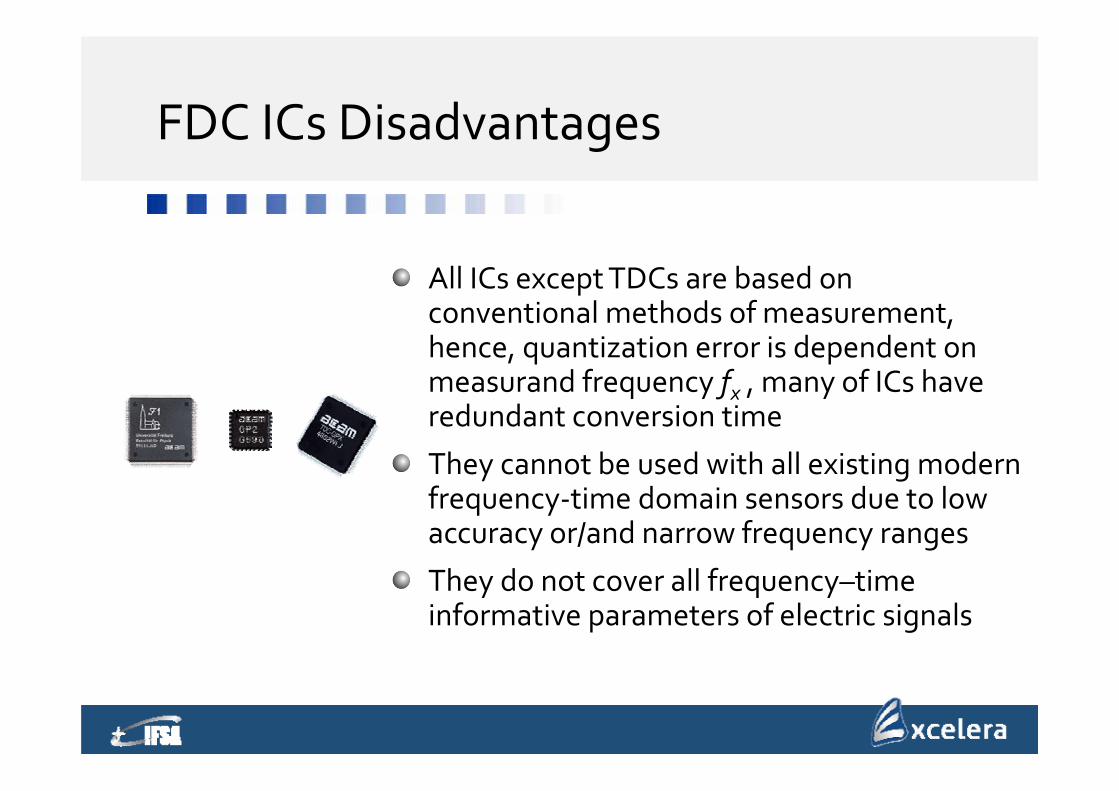
FDC ICs Disadvantages
All ICs except TDCs are based on conventional methods of measurement, hence, quantization error is dependent on measurand frequency fx , many of ICs have redundant conversion time
They cannot be used with all existing modern frequency‐time domain sensors due to low accuracy or/and narrow frequency ranges
They do not cover all frequency–time informative parameters of electric signals
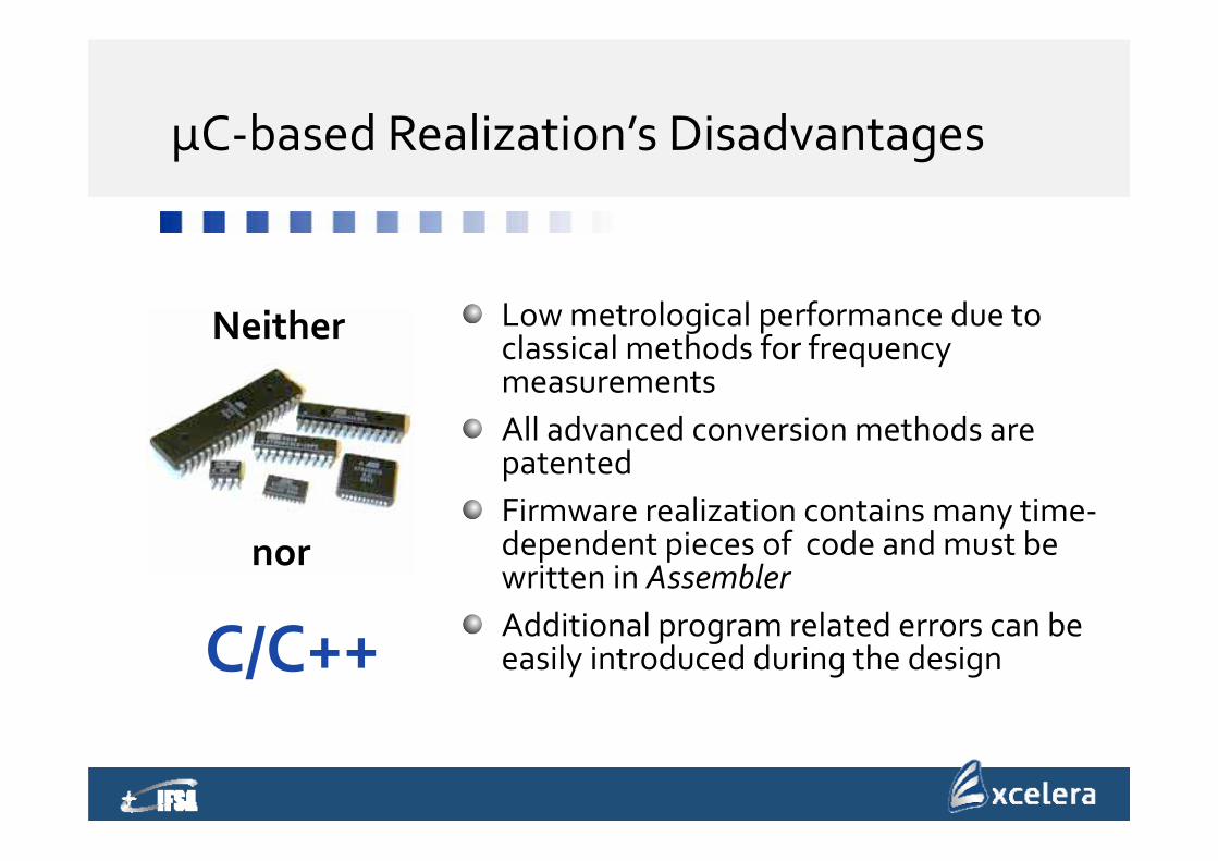
µC‐based Realization’s Disadvantages
Low metrological performance due to classical methods for frequency measurementsAll advanced conversion methods are patentedFirmware realization contains many time‐dependent pieces of code and must be written in AssemblerAdditional program related errors can be easily introduced during the designС/С++
Neither
nor
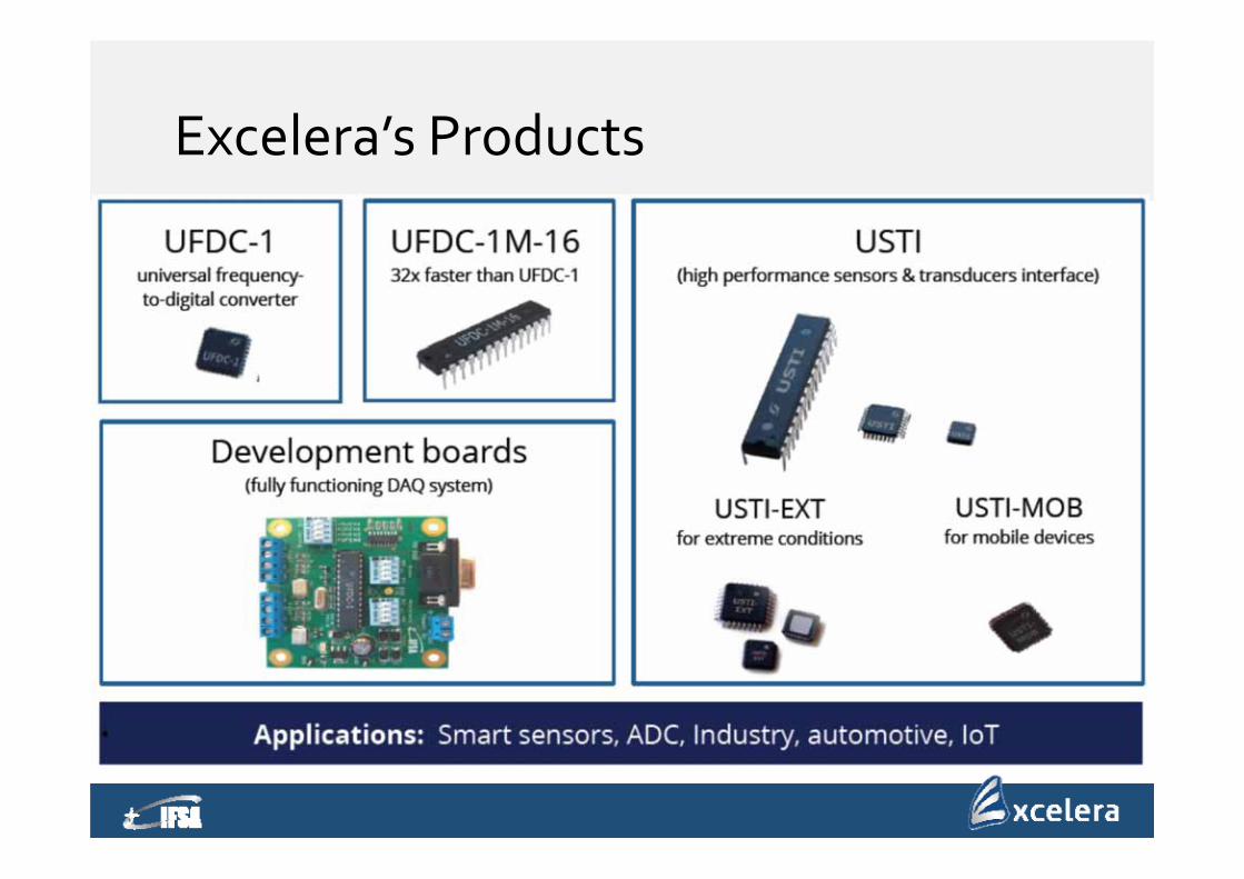
Excelera’s Products
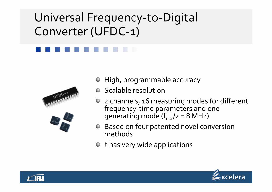
Universal Frequency‐to‐Digital Converter (UFDC‐1)
High, programmable accuracyScalable resolution2 channels, 16 measuring modes for different frequency‐time parameters and one generating mode (fosc/2 = 8 MHz)Based on four patented novel conversion methodsIt has very wide applications
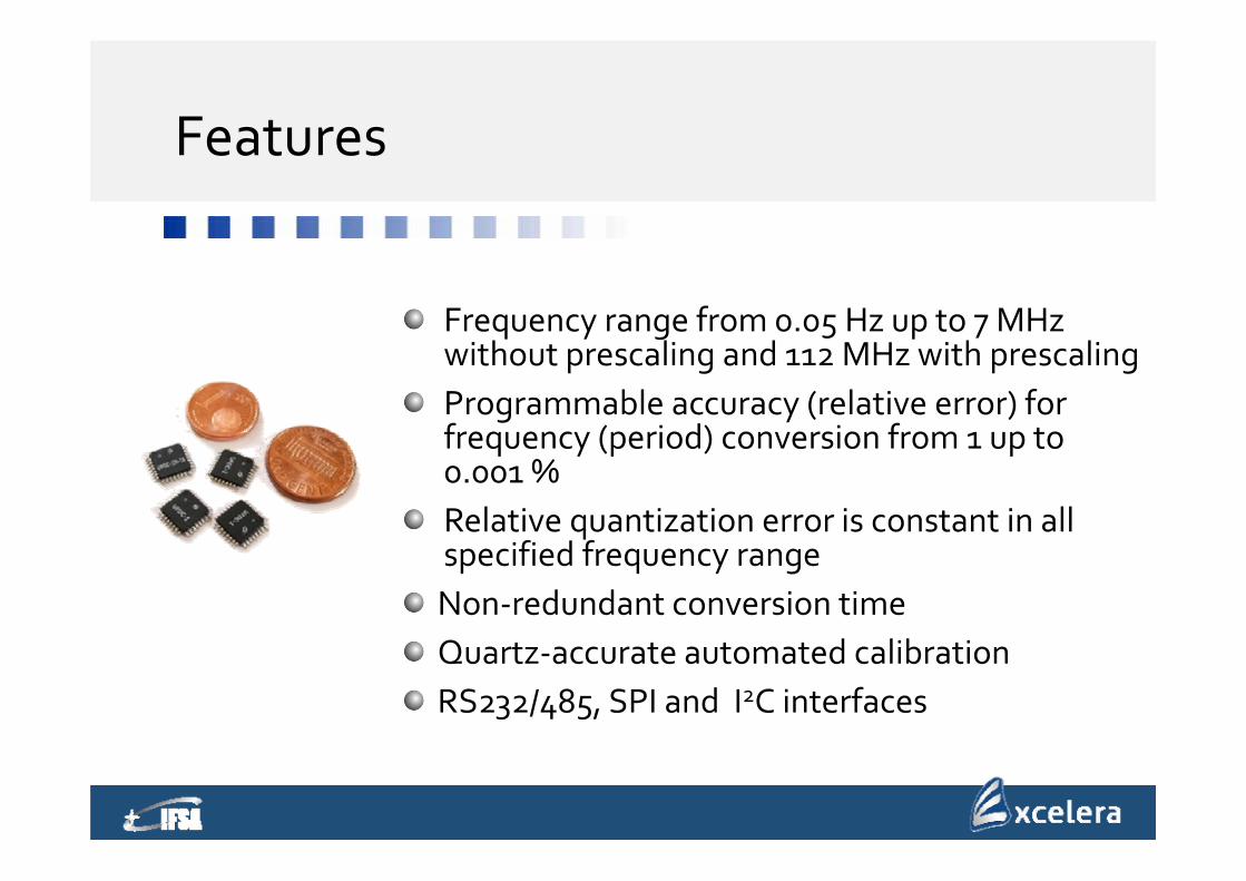
Features
Frequency range from 0.05 Hz up to 7 MHz without prescaling and 112 MHz with prescalingProgrammable accuracy (relative error) for frequency (period) conversion from 1 up to 0.001 %Relative quantization error is constant in all specified frequency range Non‐redundant conversion timeQuartz‐accurate automated calibrationRS232/485, SPI and I2C interfaces
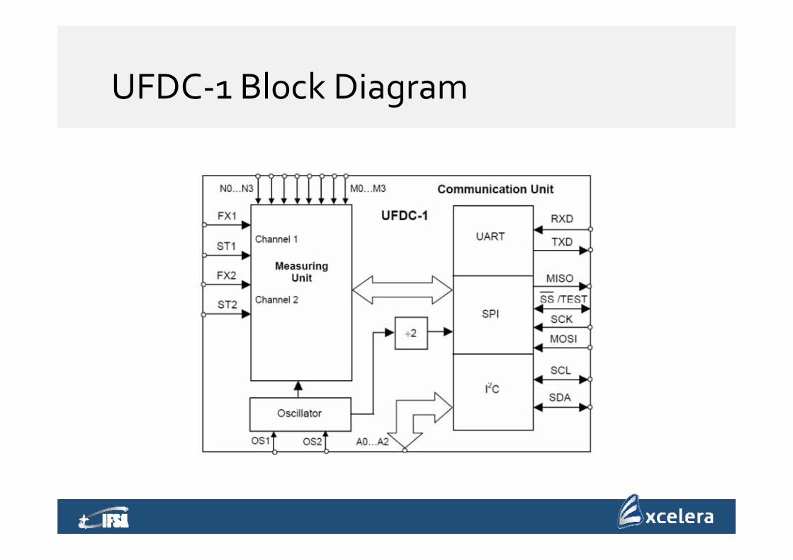
UFDC‐1 Block Diagram

Measuring Modes
Frequency, fx1 0.05 Hz – 7 MHz directly and up to 112 MHz with prescallingPeriod, Tx1 150 ns – 20 sPhase shift, x 0 ‐ 360
0 at fx 300 kHzTime interval between start‐ and stop‐pulse, x 2.5 s – 250 sDuty‐cycle, D.C. 0 – 1 at fx 300 kHz Duty‐off factor, Q 10‐8 – 8×10⁶ at fx 300 kHz Frequency and period difference and ratioRotation speed (rpm) and rotation accelerationPulse width and space interval 2.5 s – 250 sPulse number (events) counting, Nx0 – 4×10⁹
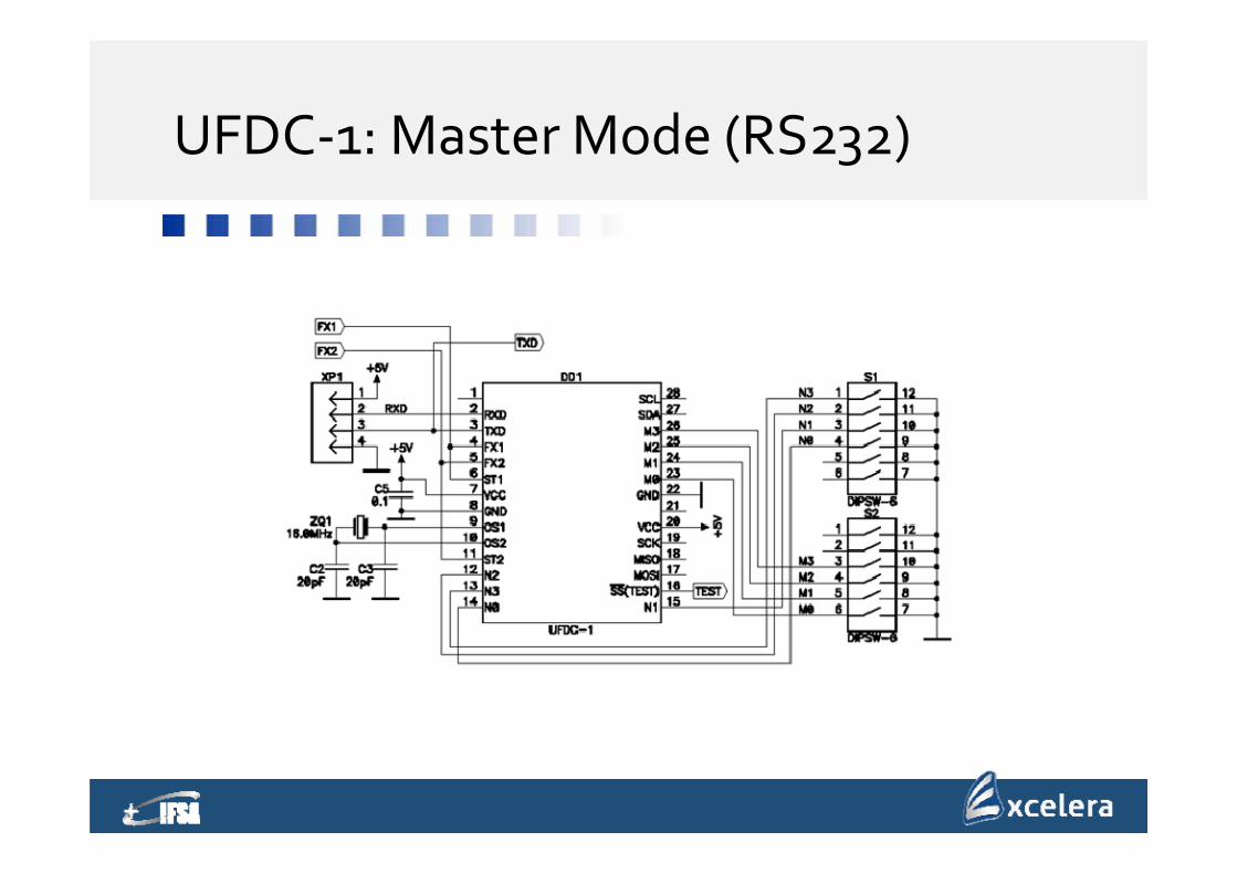
UFDC‐1: Master Mode (RS232)
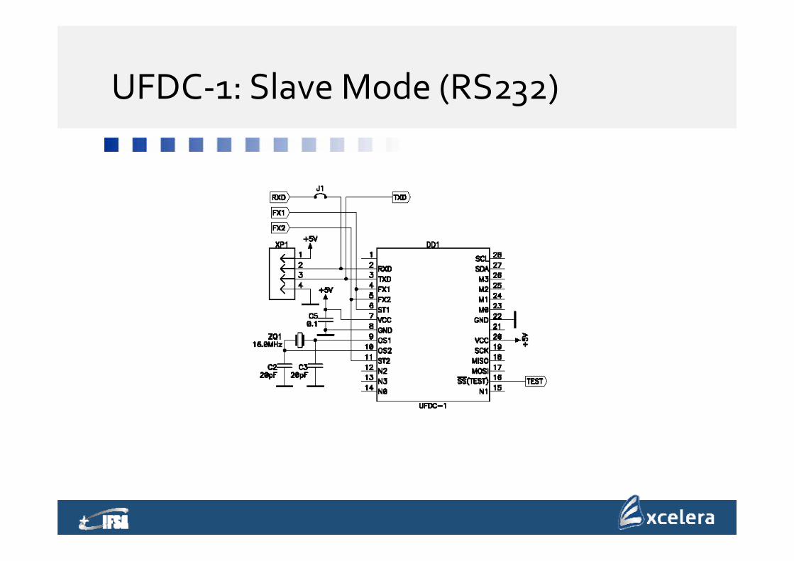
UFDC‐1: Slave Mode (RS232)

UFDC‐1: 3‐wire Serial Interface (SPI)
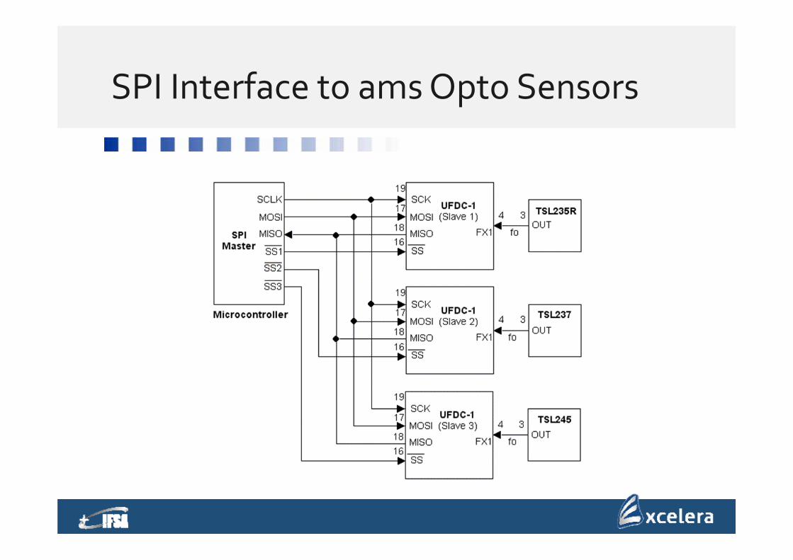
SPI Interface to amsOpto Sensors
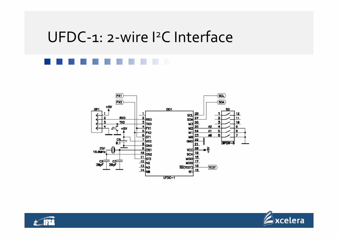
UFDC‐1: 2‐wire I2C Interface

I2C Interface to amsOpto Sensors
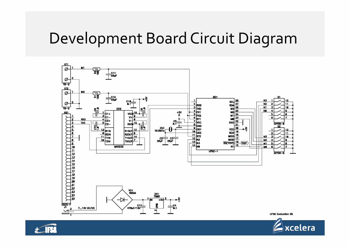
Development Board Circuit Diagram
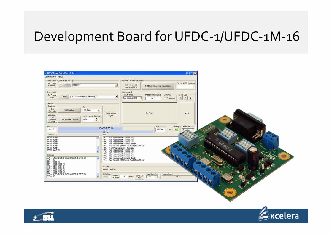
Development Board for UFDC‐1/UFDC‐1M‐16
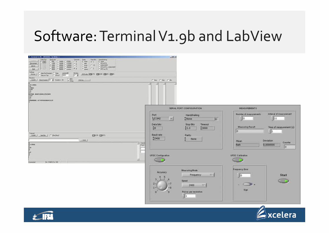
Software: Terminal V1.9b and LabView
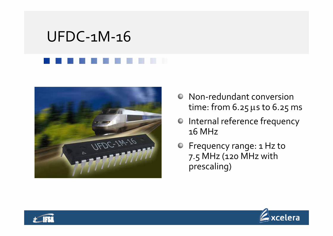
UFDC‐1M‐16
Non‐redundant conversion time: from 6.25 s to 6.25 msInternal reference frequency 16 MHz
Frequency range: 1 Hz to 7.5 MHz (120 MHz with prescaling)
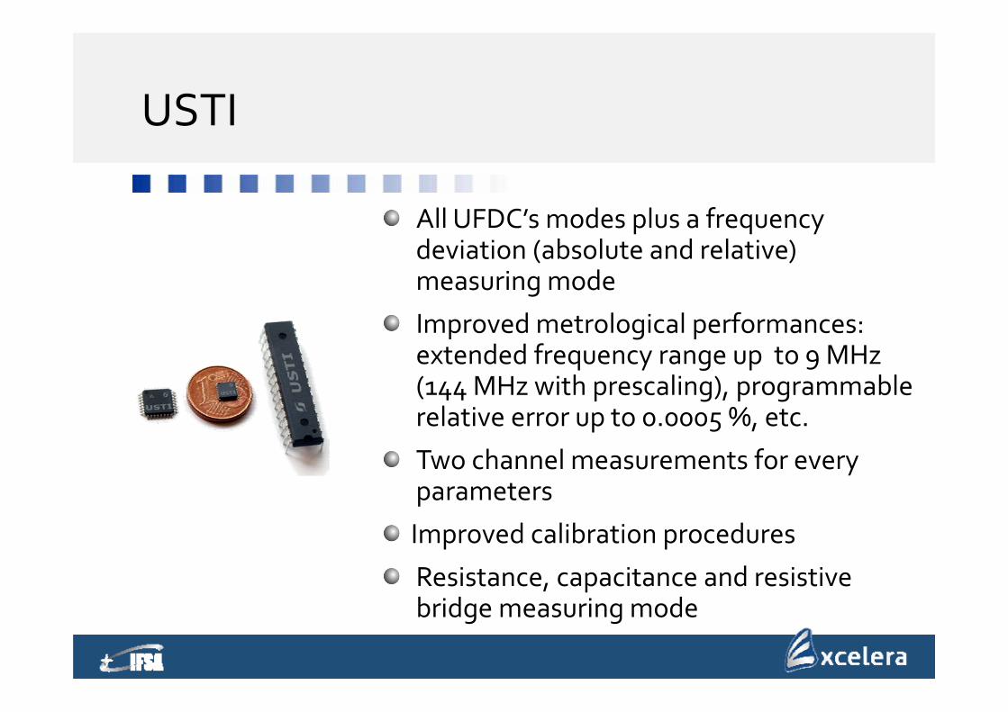
USTI
All UFDC’s modes plus a frequency deviation (absolute and relative) measuring mode
Improved metrological performances: extended frequency range up to 9 MHz (144 MHz with prescaling), programmable relative error up to 0.0005 %, etc.
Two channel measurements for every parameters
Improved calibration procedures
Resistance, capacitance and resistive bridge measuring mode
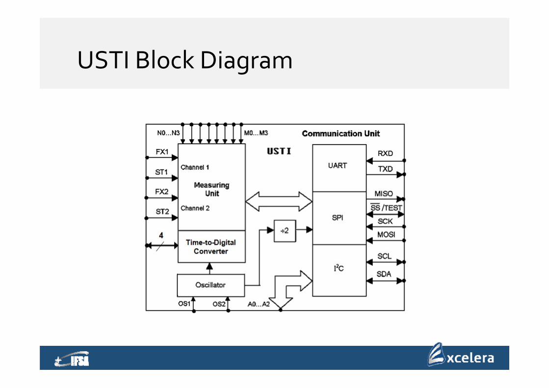
USTI Block Diagram
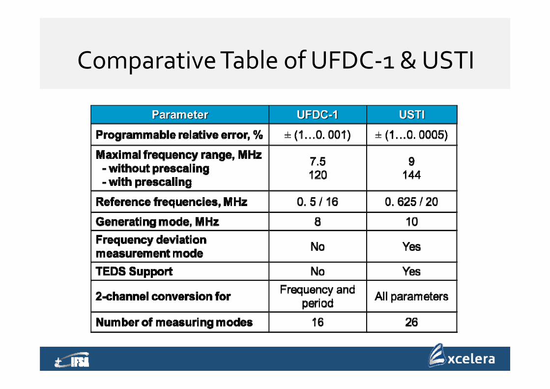
Comparative Table of UFDC‐1 & USTI
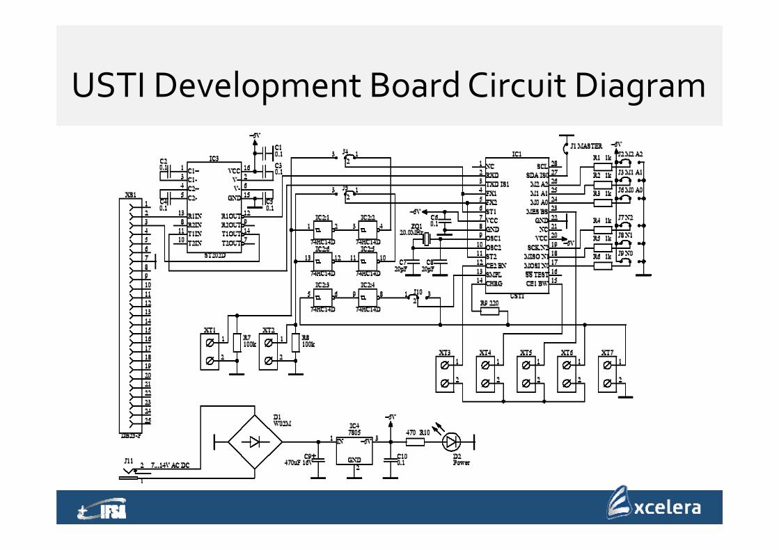
USTI Development Board Circuit Diagram
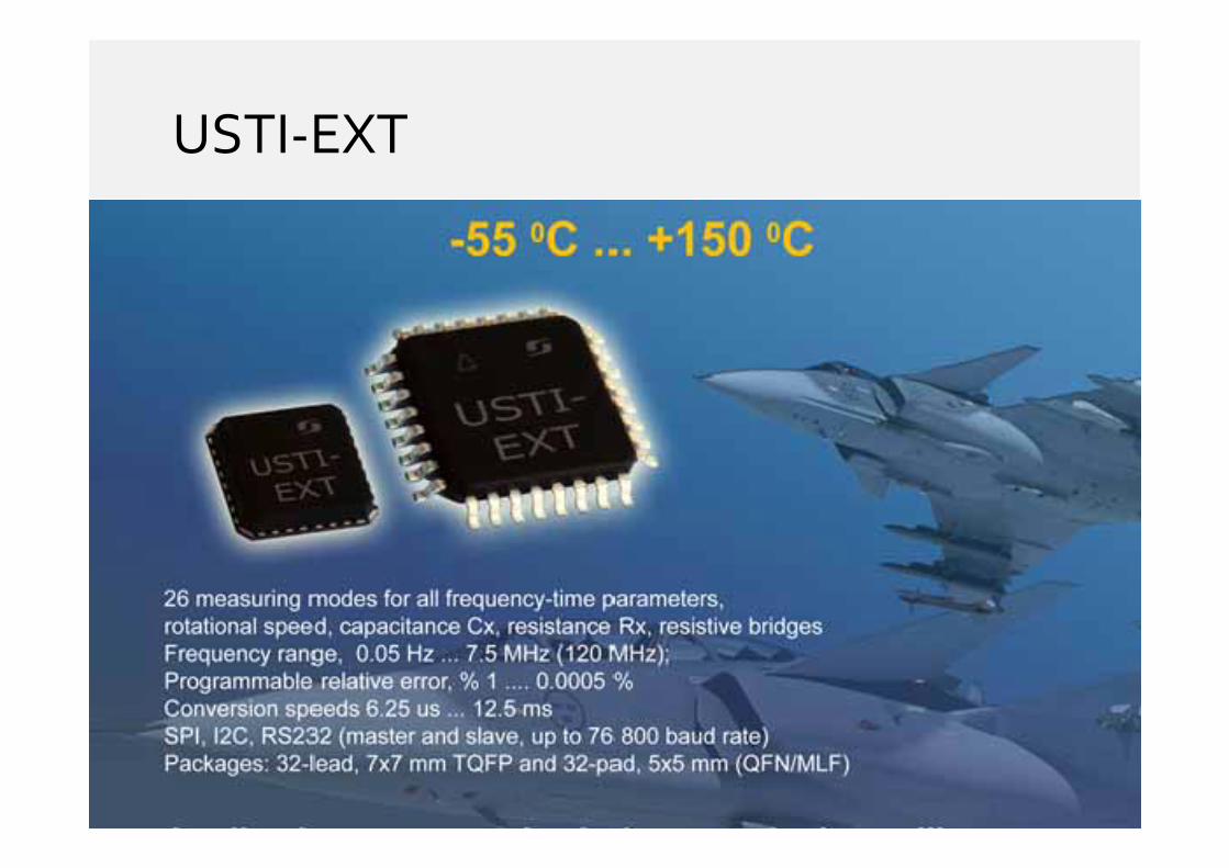
USTI‐EXT
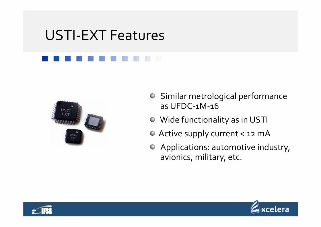
USTI‐EXT Features
Similar metrological performance as UFDC‐1M‐16
Wide functionality as in USTI
Active supply current < 12 mA
Applications: automotive industry, avionics, military, etc.
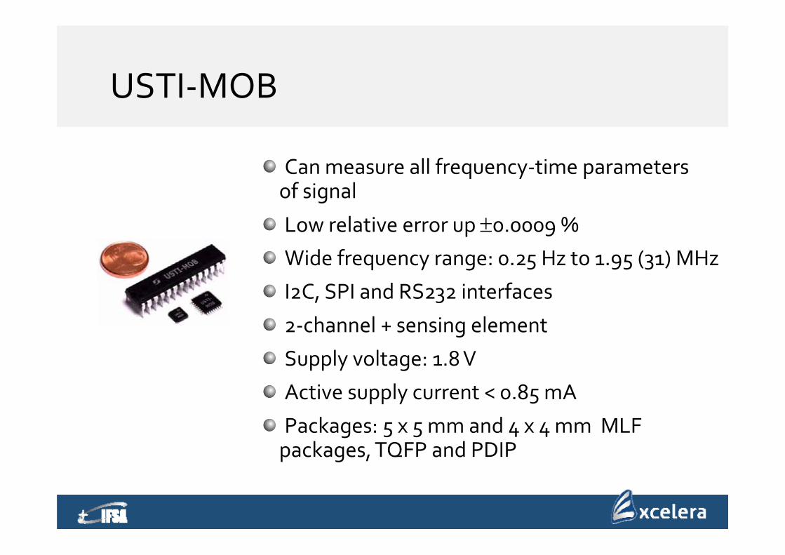
USTI‐MOB
Can measure all frequency‐time parameters of signal
Low relative error up 0.0009 %Wide frequency range: 0.25 Hz to 1.95 (31) MHz
I2C, SPI and RS232 interfaces
2‐channel + sensing element
Supply voltage: 1.8 V
Active supply current < 0.85 mA
Packages: 5 x 5 mm and 4 x 4 mm MLF packages, TQFP and PDIP
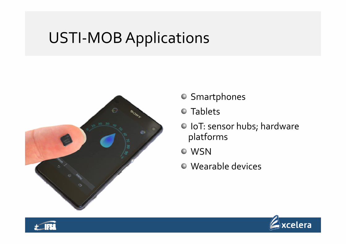
USTI‐MOB Applications
Smartphones
Tablets
IoT: sensor hubs; hardware platforms
WSN
Wearable devices
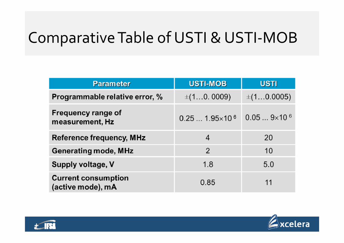
Comparative Table of USTI & USTI‐MOB
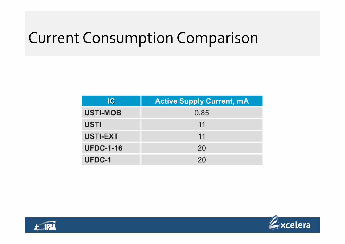
Current Consumption Comparison
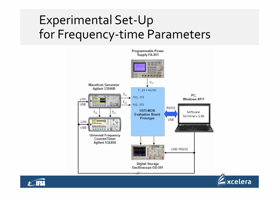
Experimental Set‐Up for Frequency‐time Parameters
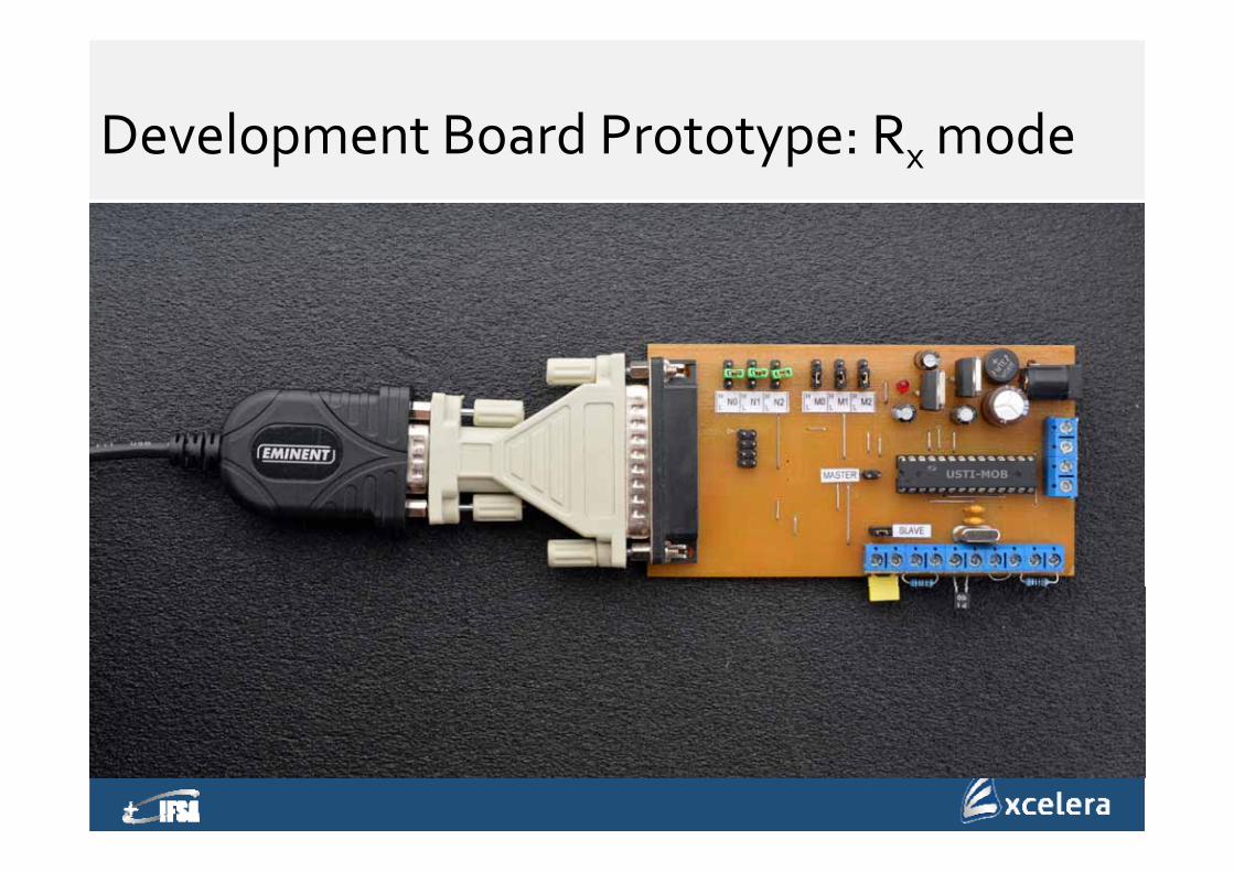
Development Board Prototype: Rx mode

Measuring Equipment
Contents
Introduction
Sensor types and classification
Advanced Design Approach
From “Smart” to “Intelligent”
Examples
Summary
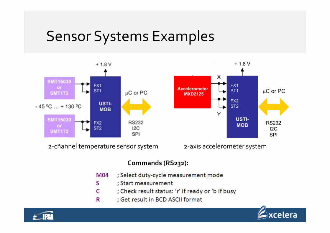
Sensor Systems Examples
2‐channel temperature sensor system 2‐axis accelerometer system
Commands (RS232):

Example: Humidity Sensor
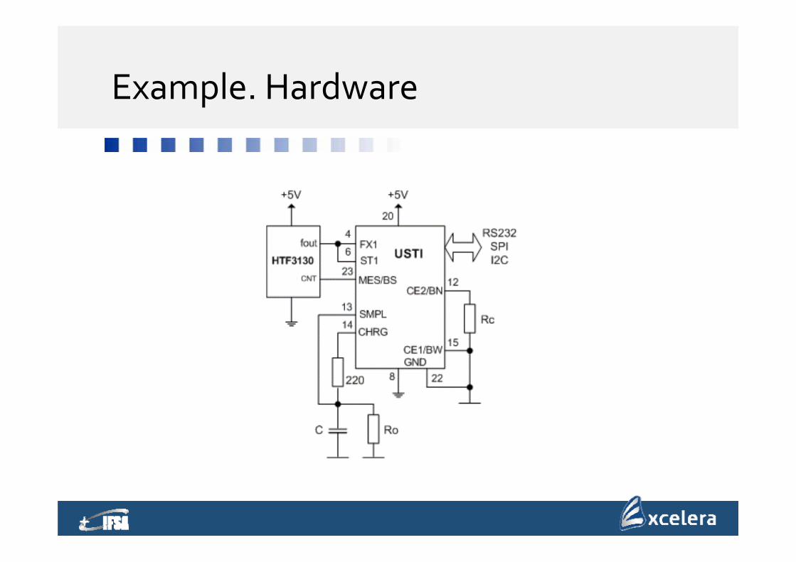
Example. Hardware
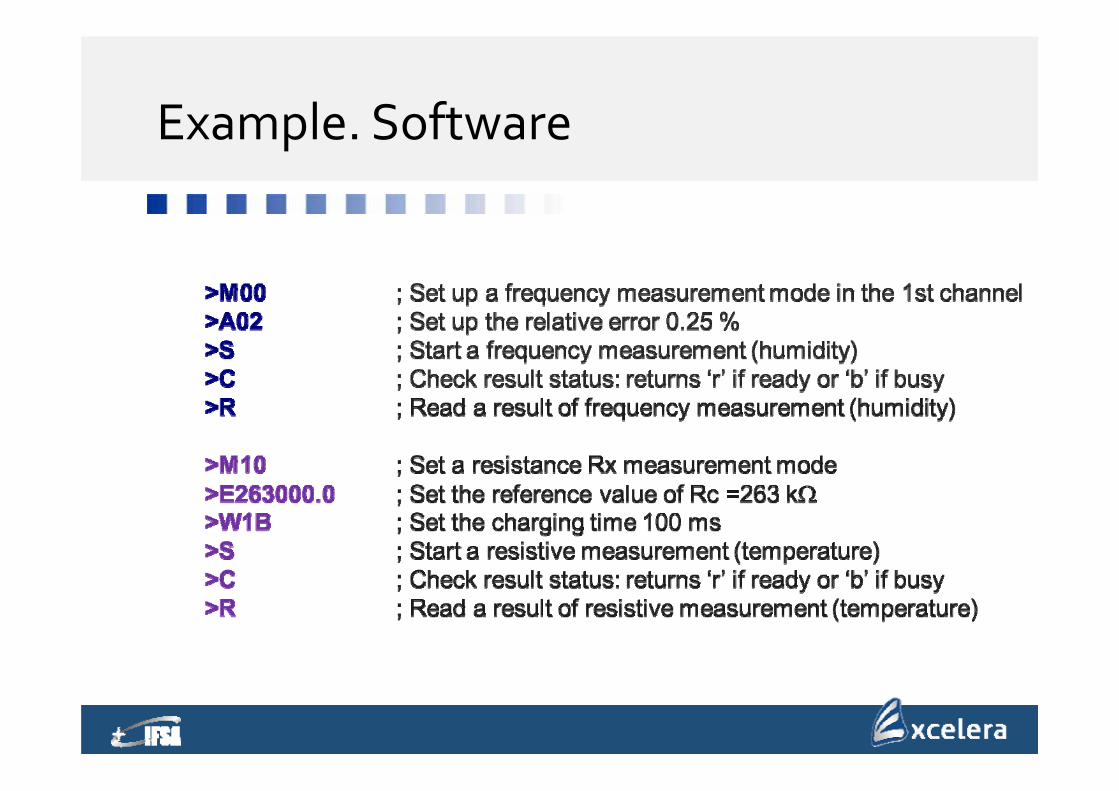
Example. Software
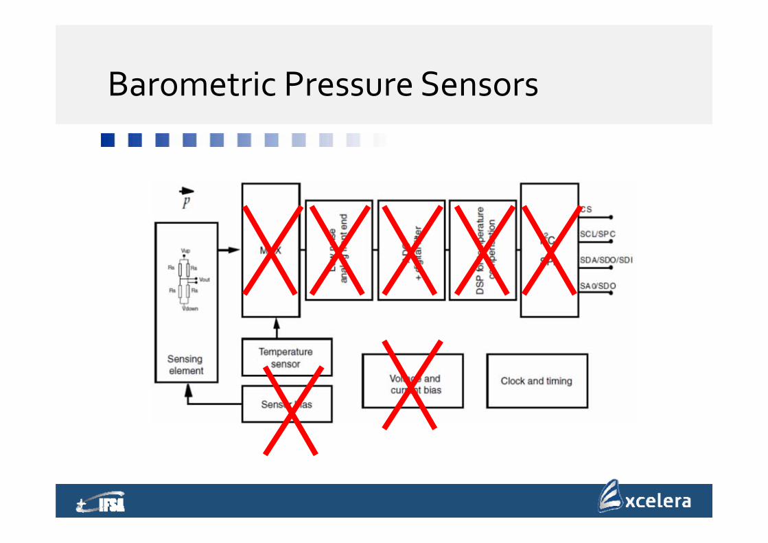
Barometric Pressure Sensors
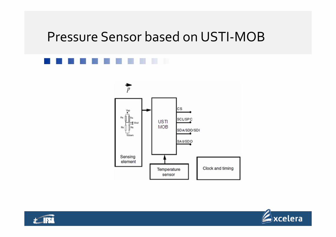
Pressure Sensor based on USTI‐MOB

Smartphone based Weather Station
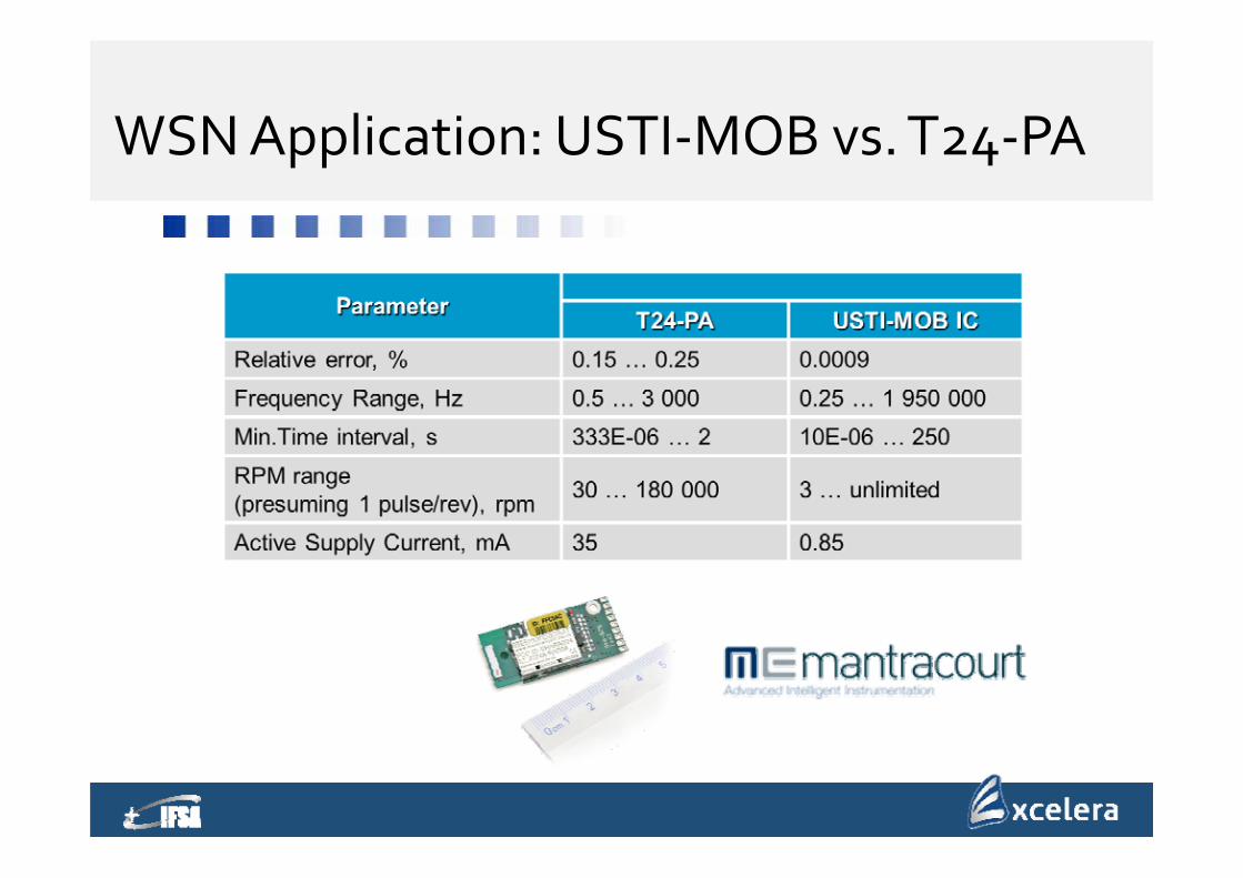
WSN Application: USTI‐MOB vs. T24‐PA
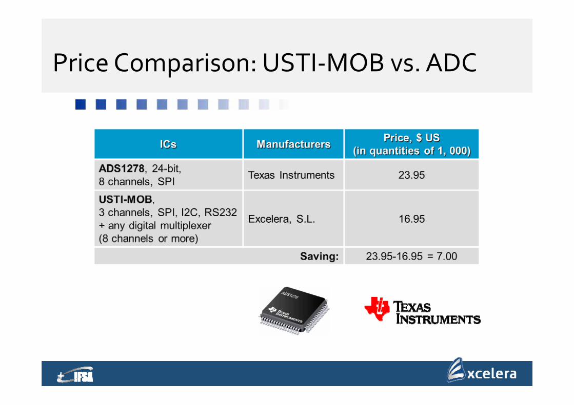
Price Comparison: USTI‐MOB vs. ADC
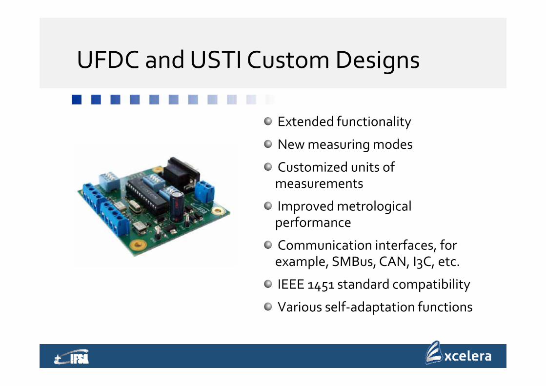
UFDC and USTI Custom Designs
Extended functionality
New measuring modes
Customized units of measurements
Improved metrological performance
Communication interfaces, for example, SMBus, CAN, I3C, etc.
IEEE 1451 standard compatibility
Various self‐adaptation functions
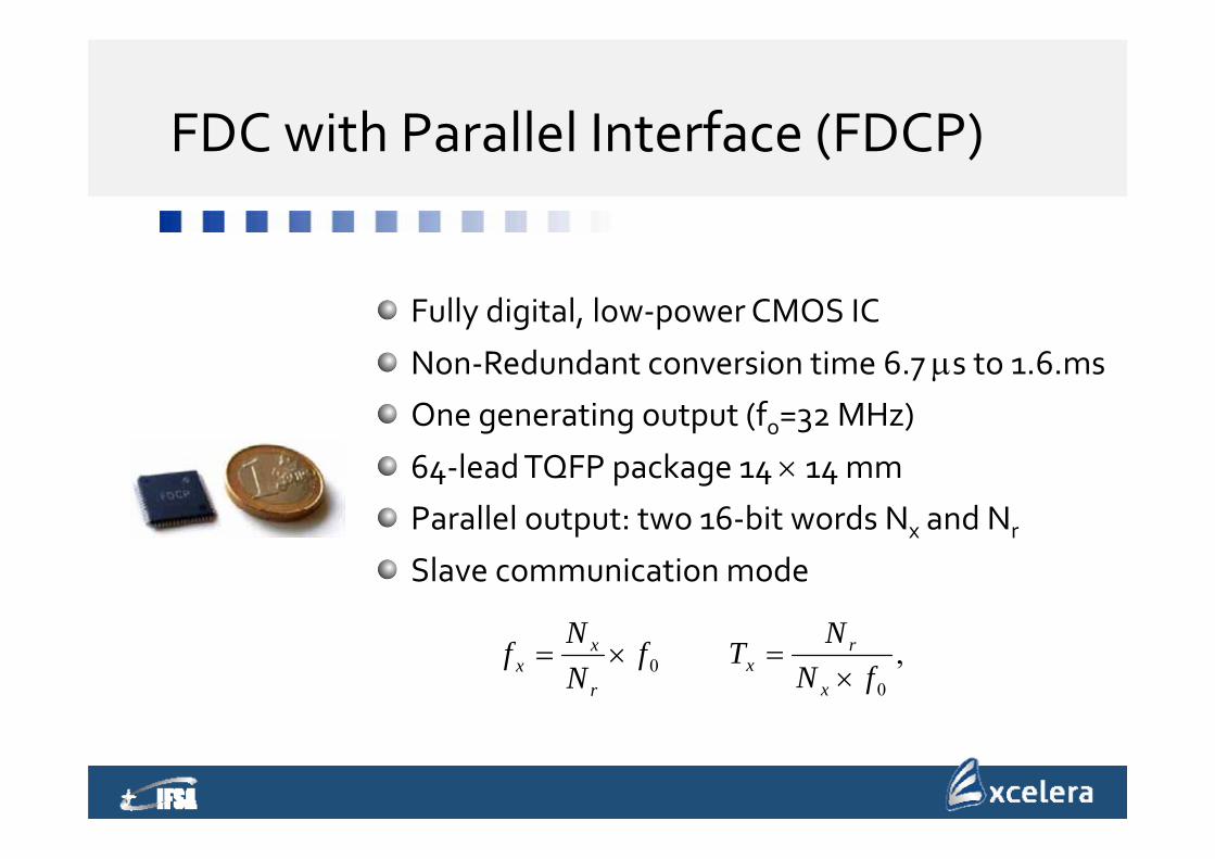
FDC with Parallel Interface (FDCP)
Fully digital, low‐power CMOS IC
Non‐Redundant conversion time 6.7 s to 1.6.msOne generating output (fo=32 MHz)
64‐lead TQFP package 14 14 mmParallel output: two 16‐bit words Nx and Nr
Slave communication mode
0fNN
fr
xx ,
0fNN
Tx
rx

FDCP Performance & Characteristics
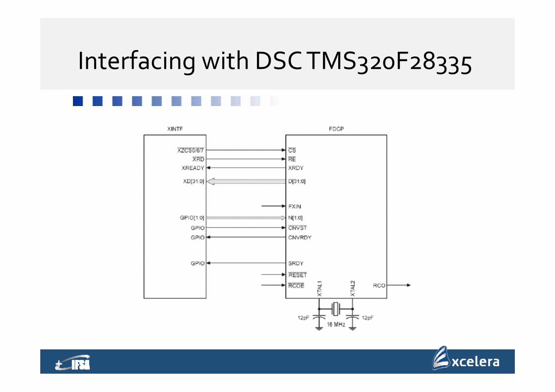
Interfacing with DSC TMS320F28335

Contents
Introduction
Sensor types and classification
Advanced Design Approach
Examples
From “Smart” to “Intelligent”
Summary
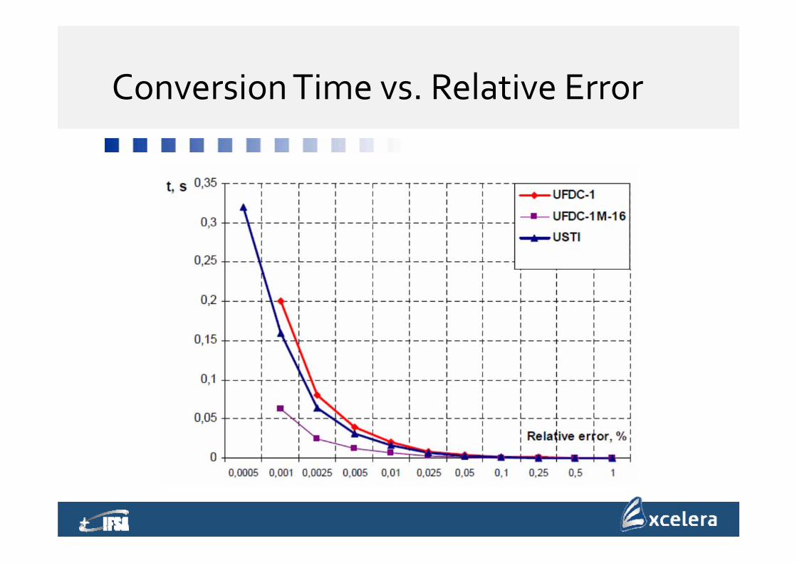
Conversion Time vs. Relative Error
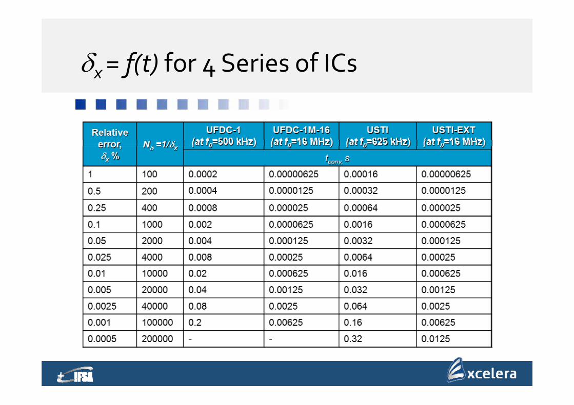
x = f(t) for 4 Series of ICs
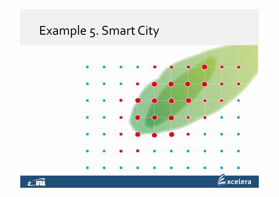
Example 5. Smart City
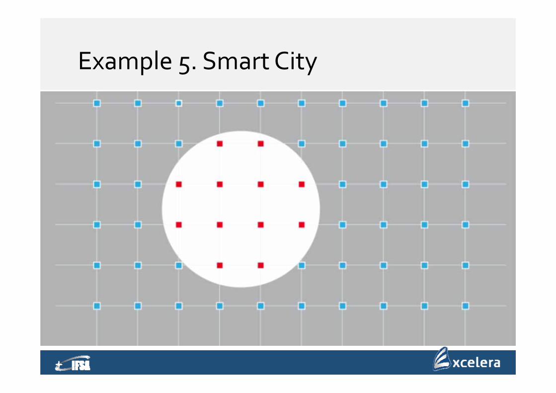
Example 5. Smart City
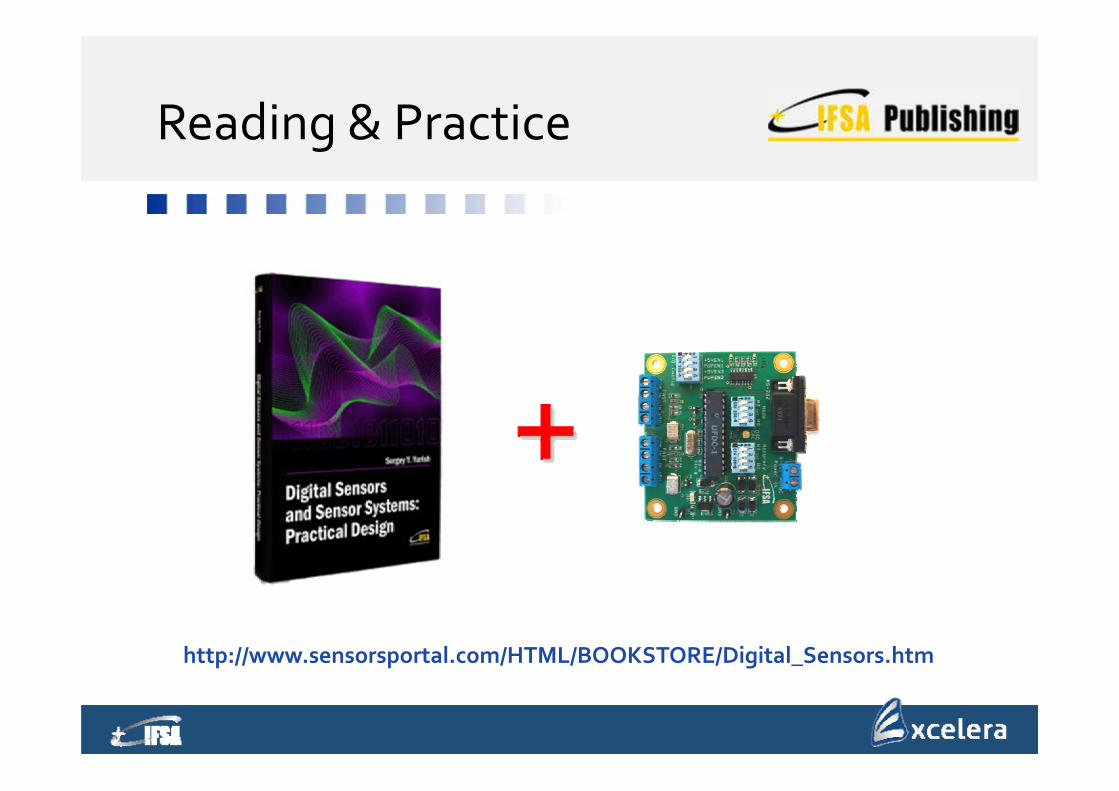
Reading & Practice
http://www.sensorsportal.com/HTML/BOOKSTORE/Digital_Sensors.htm
Summary
Quasi‐digital sensors and digital sensors on its basis are more attractive for mobile devices and IoT because of they let to eliminate current technological limitations
Proposed advanced design approach lets significantly increase a sensor system integration level and metrological performance
A lot of different sensors can be integrated by the same way in any mobile devices and IoTwithout complex sensor fusion algorithms
Contacts:
Excelera, S. L.Parc UPC‐PMT, Edifici RDIT‐K2MC/ Esteve Terradas, 108860 Castelldefels, Barcelona,SpainE‐mail: [email protected]: http://www.excelera.io


![Deep Learning With Edge Computing: A Reviewjiasi/pub/deep_edge_review.pdf · smartphones and Internet-of-Things (IoT) sensors] to a centralized location in the cloud. This potential](https://img.pdfslide.net/doc/110x75/5ec90c38aa8e8165617b222c/deep-learning-with-edge-computing-a-review-jiasipubdeepedge-smartphones.jpg)