Embed Size (px)
Citation preview
SENTIMENT ANALYSIS OF GLOBAL WARMING USING TWITTER DATA
A Paper
Submitted to the Graduate Faculty
of the
North Dakota State University
of Agriculture and Applied Science
By
Nithisha Mucha
In Partial Fulfillment of the Requirements
for the Degree of
MASTER OF SCIENCE
Major Department:
Computer Science
December 2017
Fargo, North Dakota
North Dakota State University
Graduate School
Title
SENTIMENT ANALYSIS OF GLOBAL WARMING USING TWITTER
DATA
By
Nithisha Mucha
The Supervisory Committee certifies that this disquisition complies with North Dakota
State University’s regulations and meets the accepted standards for the degree of
MASTER OF SCIENCE
SUPERVISORY COMMITTEE:
Dr. Kendall E. Nygard
Chair
Dr. Vasant Ubhaya
Dr. Limin Zhang
Approved:
04/10/2018 Dr. Kendall E. Nygard
Date Department Chair
iii
ABSTRACT
Global warming or climate change is one of the most discussed topics of the decade. Some
people think global warming is a severe threat to the planet whereas some people think, it is a
hoax. The goal of this paper is to analyze how people’s perceptions have changed over the years
for past decade using sentiment analysis on Twitter data. Twitter is a social networking platform
with 320 million monthly active users. I have captured tweets with words such as “Global
warming”, “Climate Change” etc. and applied sentiment analysis to classify them as positive,
negative or neutral tweets. I have trained Naïve Bayes Classifier, Multinomial Naïve Bayes
Classifier and SVM classifiers on several training datasets to optimize for best accuracy. The
methodology with best accuracy rate has been used to find out people’s perception of global
warming over the years using Twitter data.
iv
ACKNOWLEDGEMENTS
I would like to thank Dr. Kendall Nygard for immense support and encouragement during
my time at NDSU. I am very grateful for all the support and guidance I have received during the
research process.
I would also like to thank my Family for their wonderful support me throughout the entire
time.
v
DEDICATION
I would like to dedicate this research paper to my Family and Dr. Kendall Nygard. This paper
would not have been possible without you all. Thank you for your support and I am really
grateful for all the faith you have put in me.
THANK YOU.
vi
TABLE OF CONTENTS
ABSTRACT ................................................................................................................................... iii
ACKNOWLEDGEMENTS ........................................................................................................... iv
DEDICATION ................................................................................................................................ v
LIST OF TABLES ....................................................................................................................... viii
LIST OF FIGURES ....................................................................................................................... ix
1. INTRODUCTION ...................................................................................................................... 1
2. LITERATURE REVIEW ........................................................................................................... 3
2.1. Tweepy ................................................................................................................................. 3
2.2. Naïve Bayes Classifier ......................................................................................................... 3
2.3. Multinomial Naïve Bayes Classifier .................................................................................... 4
2.4. Support Vector Machines ..................................................................................................... 5
2.5. Parameters ............................................................................................................................ 5
2.5.1. N-gram ........................................................................................................................... 5
2.5.2. TF-IDF ........................................................................................................................... 7
2.5.3. Stopwords ...................................................................................................................... 7
2.5.4. Additive Smoothing....................................................................................................... 7
3. DATA CAPTURING AND PROCESSING .............................................................................. 9
3.1. Data Capturing Process ........................................................................................................ 9
3.2. Data Processing .................................................................................................................. 10
3.2.1. Pre-Processing ............................................................................................................. 11
3.2.2. Obtaining Stop Words List .......................................................................................... 13
3.2.3. Stemming ..................................................................................................................... 13
3.2.4. Big Picture ................................................................................................................... 14
4. TEST METHODOLOGY ......................................................................................................... 15
vii
4.1. Training Data ...................................................................................................................... 15
4.2. Testing Data ....................................................................................................................... 15
4.3. Randomness ....................................................................................................................... 15
5. RESULTS: NAÏVE BAYES CLASSIFICATION ................................................................... 17
5.1. Unigram Implementation ................................................................................................... 17
5.2. Bigram Implementation ...................................................................................................... 17
5.3. Test Accuracy ..................................................................................................................... 17
6. RESULTS: MULTINOMIAL NAÏVE BAYES CLASSIFIER ............................................... 18
6.1. N-gram Iterations ............................................................................................................... 18
6.2. N-gram Iterations ............................................................................................................... 20
6.3. N-gram Iterations with TF-IDF and Alpha Smoothing Parameter..................................... 21
6.4. Tuning Alpha Parameter Value .......................................................................................... 21
7. SUPPORT VECTOR MACHINES .......................................................................................... 23
7.1. Support Vector Classification -Linear Classifier ............................................................... 23
7.2. Linear Support Vector Classification ................................................................................. 24
7.3. Linear Support Vector Classification ................................................................................. 25
8. SUMMARY OF TEST CASES ................................................................................................ 27
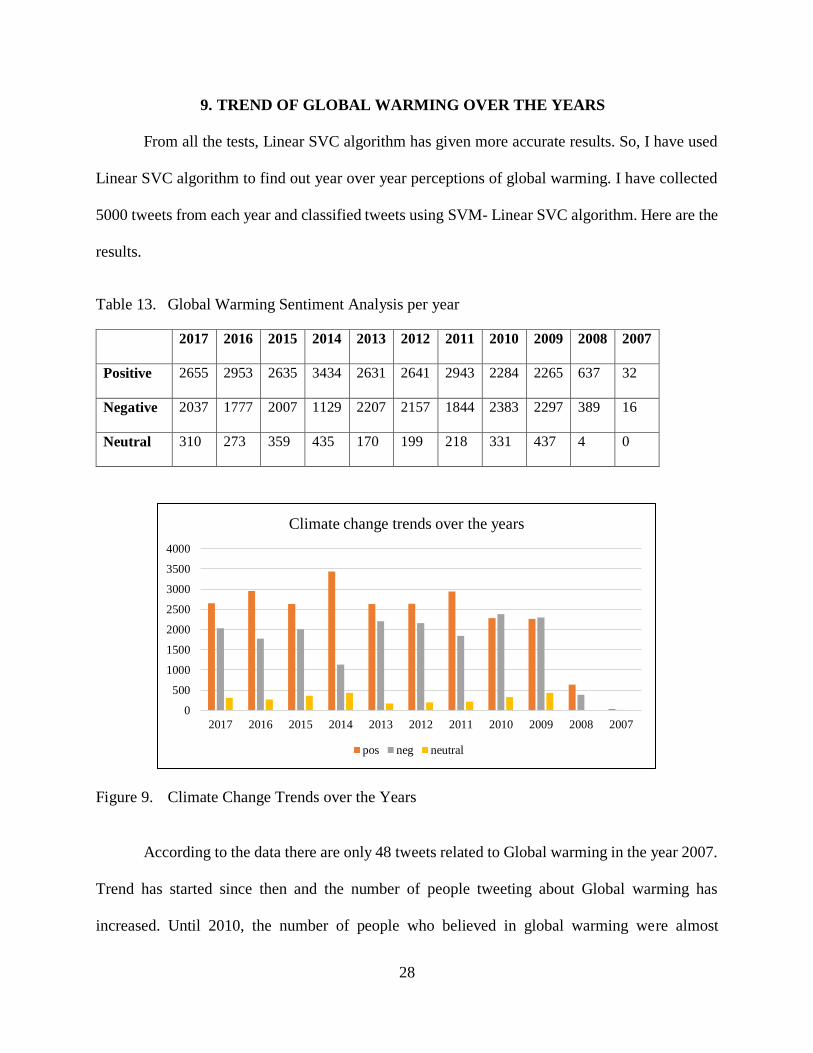
9. TREND OF GLOBAL WARMING OVER THE YEARS ...................................................... 28
10. CONCLUSION AND FUTURE WORK ............................................................................... 30
REFERENCES ............................................................................................................................. 31
viii
LIST OF TABLES
Table Page
1. Tweets Classification Example ............................................................................... 10
2. Unigram vs. Bigram NLTK .................................................................................... 17
3. Best Case Summary Step 1 ..................................................................................... 17
4. Index Description .................................................................................................... 18
5. Best Case Summary Step 2 ..................................................................................... 19
6. Best Case Summary Step 3 ..................................................................................... 20
7. Best Case Summary Step 4 ..................................................................................... 21
8. Best Case Summary Step 5 ..................................................................................... 22
9. Best Case Summary Step 6 ..................................................................................... 23
10. Effect of Various Kernels in SVC on Accuracy ..................................................... 24
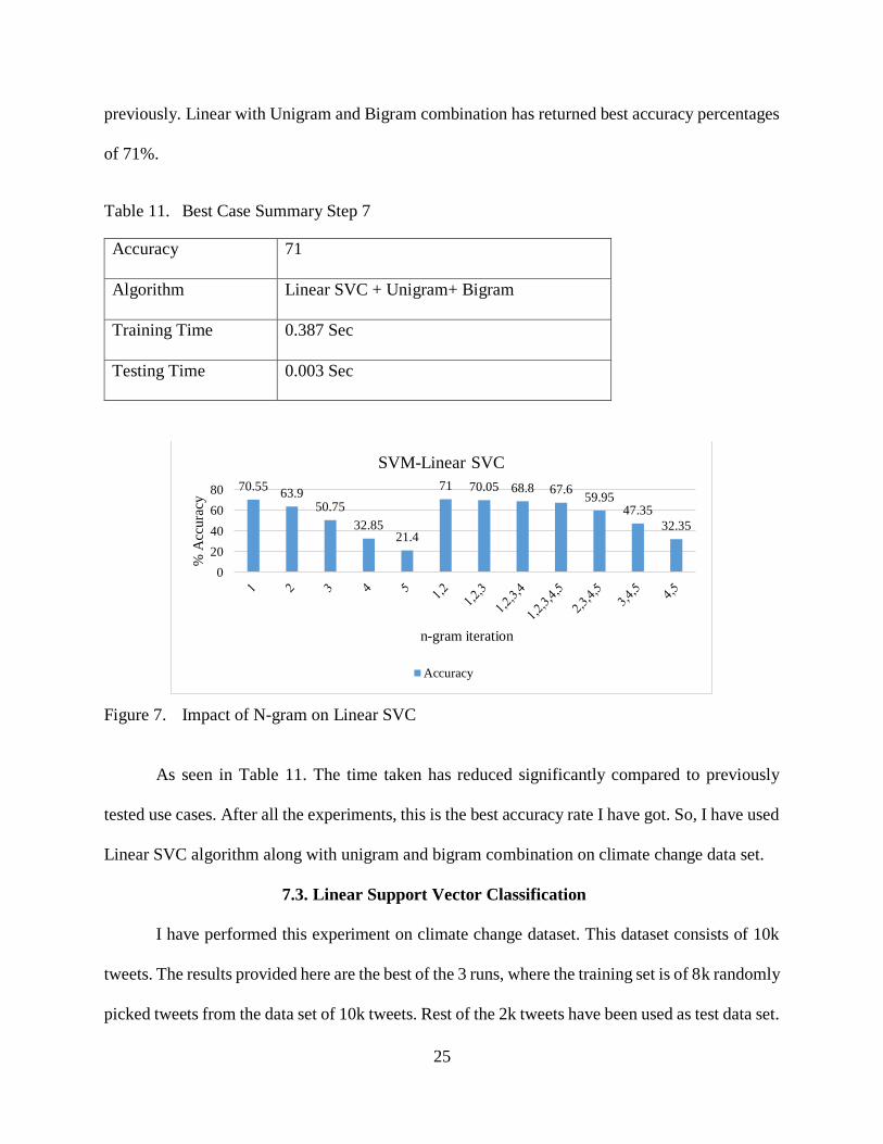
11. Best Case Summary Step 7 ..................................................................................... 25
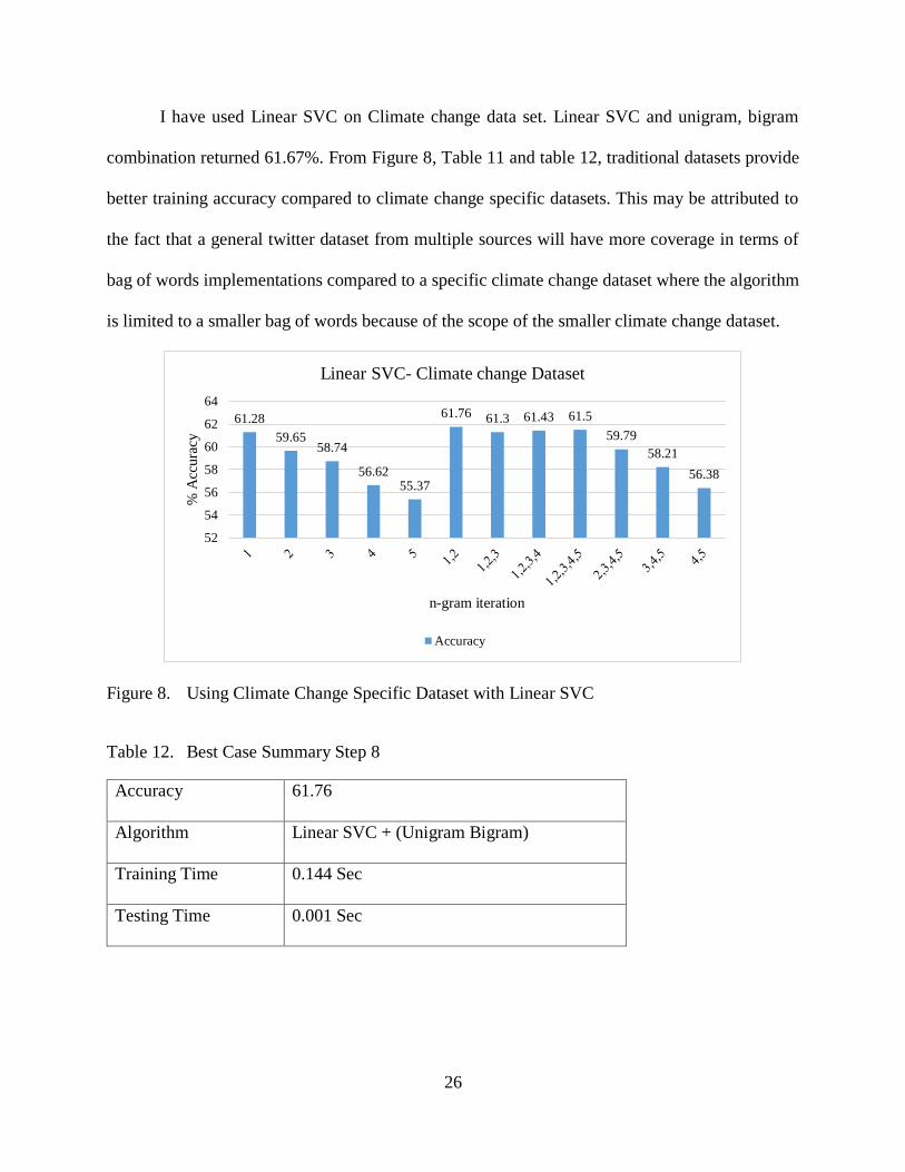
12. Best Case Summary Step 8 ..................................................................................... 26
13. Global Warming Sentiment Analysis per year ....................................................... 28
ix
LIST OF FIGURES
Figure Page
1. Example Code Tweet Retrieval .................................................................................. 10
2. Impact of n-gram on Accuracy with Multinomial NB ............................................... 19
3. Custom Stopwords vs. NLTK Corpus Stopwords ...................................................... 20
4. Impact of Smoothing Parameter (alpha) on Accuracy ............................................... 21
5. Tuning Smoothing Parameter ..................................................................................... 22
6. Impact of N-gram on Accuracy with SVM-SVC-Linear kernel ................................ 24
7. Impact of N-gram on Linear SVC .............................................................................. 25
8. Using Climate Change Specific Dataset with Linear SVC ........................................ 26
9. Climate Change Trends over the Years ...................................................................... 28
1
1. INTRODUCTION
Global warming is also referred to as climate change and the greenhouse effect. When CO2
and other pollutant gases produced by several sources such as automobiles and industries are
released into earth’s atmosphere, they eventually flow into space. However, as the production of
these gases raises, they get trapped on the earth surface. While on the earth surface, gases like CO2
absorb sun’s radiation. Thus, the temperature of the earth has been increasing in the past several
decades. This phenomenon is called global warming. Over the years earth’s average temperatures
have been increased and gradually ocean levels are rising due to melting glacial polar caps. Most
of the scientists believe in global warming whereas few scientists believe global warming is a hoax
and it’s a natural process. The split of the general population who believe in global warming vs
those who don’t have been changing throughout the years.
Extreme weather conditions like frequent hurricanes, floods, drought and long heatwaves
are developing in recent years. Frozen lakes are melting earlier than expected due to warmer
winters. According to scientists, 2000-2009 is the hottest decade than any other decade in past
1300 years. The dry places are becoming dryer and wet places are becoming wetter. Earth’s
geography and climate systems have been changing in an irreparable way. According to scientific
studies, earth’s temperatures will rise by 8 degrees by 2100[1][2][3].
Twitter is a social media platform with 328 million monthly active users [6]. Since its
advent, it has been the best platform to collect people’s opinions about various topics like games,
politics, entertainment, social causes, global warming etc. In this paper, I used Twitter data to
understand the trends of user’s opinions about global warming and climate change using sentiment
analysis. I have trained various classification algorithms and tested on generic Twitter datasets as
well as climate change specific datasets to find a methodology with the best accuracy. Finally, I
2
have captured 5000 tweets for each year in the last decade and used the best classifier to classify
tweets into positive, negative and neutral classes. The goal of this paper is to find out how people’s
perception of global warming has changed over last 10 years. Positive, neutral classes are defined
as below.
Positive = People who think global warming is true
Negative = People who think global warming is hoax
Neutral = Neither positive nor negative
Rest of the paper has been arranged as follows. In the subsequent sections, we discuss
classifiers such as Naïve Bayes from NLTK platform, Multinomial Naïve Bayes Classifier,
Support Vector Machines (SVM) and different types of SVM from the Scikit platform. We look
into parameters like TF-IDF, N-gram, stop words and tools like Tweepy. I have explained data
capturing and data processing steps in section three. Test methodology has been explained in the
fourth section. I have listed test results for NLTK Naïve Bayes classifier with graphs in the fifth
section. Sixth section and seventh section describe Scikit Multinomial Naïve Bayes and SVM
classifier test results respectively. The eighth section is the comparison of all the classifiers and
test results and summarizing the best classification method from all the experimentation done in
previous sections. The ninth section contains classification results for twitter data from past ten
years pertaining to climate change using the classifier with best accuracy rate. The tenth section
refers to the conclusion and future work.
3
2. LITERATURE REVIEW
This section outlines the technologies and methodologies used in this study in detail. It also
dwells on the Algorithms and their parameters used in related contemporary studies.
2.1. Tweepy
Tweepy is an open source python library as mentioned in [4], which enables python to
communicate with Twitter and access its Application Programming Interface (API). Capturing real
time as well as historic Twitter data is easier using Tweepy. Tweepy along with other libraries
developed by developers are used towards performing various services on Twitter [6].
2.2. Naïve Bayes Classifier
Naïve Bayes Classifier is a basic classifier in machine learning. It is an efficient
classification method in NLTK (Natural Language Processing Tool Kit) [5]. This classifier works
better with Textual contents.
During training, the classifier goes through all text documents and defines the probability
of the words being positive, negative and neutral and then compares it to the label of the tweet
which is the sentiment in this case. It is based on Bayes theory assuming all variables are
independent. I.e. Every feature being classified are independent of the value of other features in
the document. This is very efficient classifier and suitable for very large data sets classification.
Naïve Bayes classifier is also good with real-time and multi-class classification. Naïve Bayes
classifier works efficiently for sentiment analysis on social media like twitter. So, I have chosen
Naïve Bayes classifier as one of the classifiers for Global warming Twitter sentiment analysis.
According to Bayes theorem [16][19]
The terms above are defined as follows:
4
P(A/B) = Probability of A given B
P(B/A) =Probability of B given A
P(A) = Probability of A
P(B) = Probability of B
2.3. Multinomial Naïve Bayes Classifier
Multinomial Naïve Bayes classifier is one of the classifiers in SciKit-learn library. It is an
enhancement compared to the Naïve Bayes classifier and also is a very efficient classifier.
Multinomial Naïve Bayes classifier is the probabilistic classification method where Probability of
a class given in a document depends on the prior probability of features appeared in the class
whereas in Naïve Bayes classifier each feature is treated as independent of one another. This is the
main difference between Naïve Bayes classifier and Multinomial Naïve Bayes classifier [17][
14][13].
In this paper, I have used multinomial Naïve Bayes classifier with stop words, multiple n-
gram iterations and also with smoothing factor alpha. Results are explained clearly in section 6.
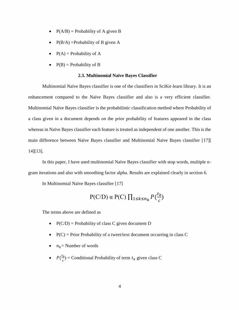
In Multinomial Naïve Bayes classifier [17]
P(C/D) α P(C) ∏ 𝑃(𝑡𝑘
𝑐1≤𝑘≤𝑛𝑘 )
The terms above are defined as
P(C/D) = Probability of class C given document D
P(C) = Prior Probability of a tweet/text document occurring in class C
𝑛𝑘= Number of words
𝑃(𝑡𝑘
𝑐) = Conditional Probability of term 𝑡𝑘 given class C
5
2.4. Support Vector Machines
Support Vector Machines is an effective machine learning algorithm used for classification
and regression use cases. Most of the times SVM is used for classification. It segregates classes
by finding the best hyperplane between different classes. Support Vector Machines has different
kernel functions which can be used towards creating the best model to find the hyperplane. The
kernel functions are Poly, Sigmoid, Linear, and rbf. For this paper, I have used all kernel functions
to find the best classification hyperplane. C-support vector classification and Linear Support vector
classification have been used as well in this paper. Linear support vector classification is similar
to Support Vector classification using the linear algorithm. However, Linear Support Vector
machines are more flexible in penalties and losses. So Linear Support Vector classification works
efficiently for larger data sets as mentioned in [18][20][28]
2.5. Parameters
Below parameters are used along with Naïve Bayes classifier, Multinomial Naïve Bayes
classifier, and Support vector machines classifiers. Using the parameters like stop words, n-gram
and TF-IDF, additive smoothing has notable impacts on the experiment results.
2.5.1. N-gram
Language modeling is a probability distribution of a combination of the words. N-gram is
one of the methods in language modeling where text documents can be divided into a combination
of sequential words. Data from the text document can be divided into n-grams and combination of
N-grams. This set of n-grams will be used towards training the algorithms. [0][12]
2.5.1.1. Unigram
Text document can be divided into single words. In n-gram, n refers to the number of
words. If the size of the gram is 1, it is called unigram. [0][12]
6
Ex: Climate change is causing a rise in ocean temperatures.
Using unigram, the above sentence can be divided into the following (Climate, change, is, causing,
rise, in, ocean, temperatures)
Stop words such as “is”, “in”, “are” etc. do not contribute to the probability distributions
of sentiment analysis. To get a better range of feature vectors, bigram and trigram are better suited.
2.5.1.2. Bigram
If the size of n is equal to two, it is called bigram. [0][12]
Ex: Climate change is causing a rise in ocean temperatures.
In bigram above sentence can be divided into ((Climate, change), (Change, is), (is,
causing), (causing, rise), (rise, in), (in, ocean), (ocean, temperatures))
2.5.1.3. Trigram
If the size of n is equal to three, it is called trigram. [0][12]
Ex: Climate change is causing a rise in ocean temperatures.
Above sentence in trigrams ((climate, change, is), (change, is, causing), (is, causing, rise),
(causing, rise, in), (rise, in, ocean), (in, ocean, temperatures))
2.5.1.4. Four-gram
If the size of n is equal to four, it is called four-gram. [0][12]
Ex: Climate change is causing a rise in ocean temperatures.
Above sentence in four-grams ((climate, change, is, causing), (change, is, causing, rise),
(is, causing, rise, in), (causing, rise, in, ocean), (rise, in, ocean, temperatures))
2.5.1.5. Five-gram
If size of n is equal to five, it is called five-gram. [0][12]
Ex: Climate change is causing rise in ocean temperatures.
7
Above sentence in five-grams ((climate, change, is, causing, rise), (change, is, causing,
rise, in), (is, causing, rise, in, ocean), (causing, rise, in, ocean, temperatures))
2.5.2. TF-IDF
TF-IDF stands for term frequency Inverse document frequency. It is a basic classification
method to determine the weight of the terms in the given document. Stop words such as “is, it,
that, them” etc. which don’t add much in terms of sentiment analysis of the tweet will be neglected
in this classification to determine accurate term weight. In this paper, I have used TF-IDF with
Multinomial Naïve Bayes classifier. Accuracy has not improved much when minimum term
frequency or document frequency are set in this case since we are dealing with Twitter data which
consists of a few words per instance rather than a corpus which consists of several large documents.
We iteratively experimented with minimum term frequencies and document frequencies set to
various values ranging from 5 to 2000 without much significant change in accuracy. TF- IDF gives
good results with larger text documents where chances of word repetitions are frequent. [7]
TF(term)= Number of time term appeared in the document/Number of total terms in the document
and IDF(term)= Log_e (total number of documents/Number of times term in it)
2.5.3. Stopwords
Stop words are the words which don’t add much weight to the sentence and don’t have
much significance. During the classification, removing stop words will save a significant amount
of time in terms of computation. Usually, stop words add a lot of unnecessary weight during the
classification process. Removing them from tweets will improve the accuracy. [29]
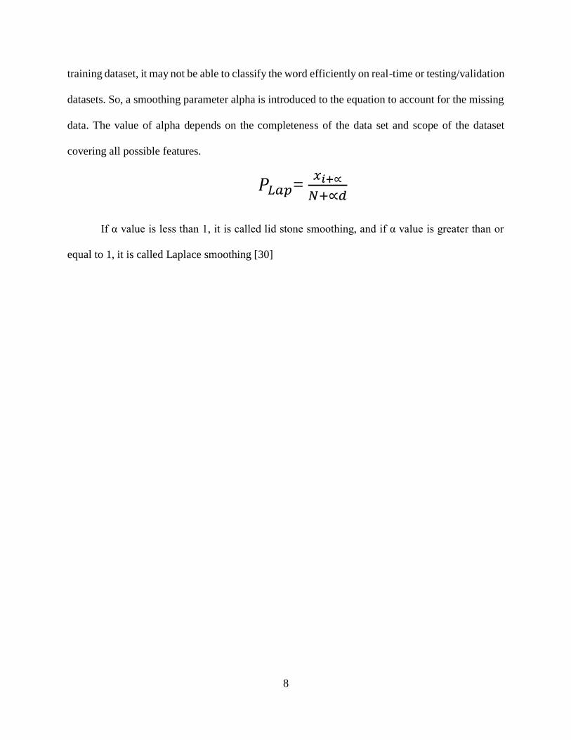
2.5.4. Additive Smoothing
Additive smoothing or Laplace and Lid stone smoothing are introduced to avoid overfitting
during the classification process. When algorithm has to classify a new word, which is not in the
8
training dataset, it may not be able to classify the word efficiently on real-time or testing/validation
datasets. So, a smoothing parameter alpha is introduced to the equation to account for the missing
data. The value of alpha depends on the completeness of the data set and scope of the dataset
covering all possible features.
𝑃𝐿𝑎𝑝= 𝑥𝑖+∝
𝑁+∝𝑑
If α value is less than 1, it is called lid stone smoothing, and if α value is greater than or
equal to 1, it is called Laplace smoothing [30]
9
3. DATA CAPTURING AND PROCESSING
3.1. Data Capturing Process
Twitter streaming API is used to capture the data. Twitter streaming API helps to make
connection between computer programs and web services. For accessing Twitter streaming API
we need four keys called API Key, API Secret, Access Token, and Access Token Secret.
Steps to retrieve four keys
Create a Twitter account
Open page https://apps.twitter.com/ and login with twitter credentials
Try creating a new app
Fill the form and ‘Create twitter new application’
Retrieve API keys and API secret
Retrieve access token and Access token secret.
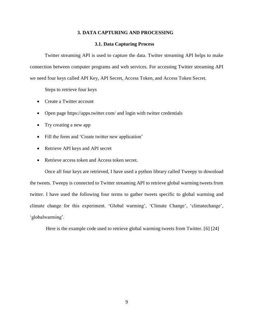
Once all four keys are retrieved, I have used a python library called Tweepy to download
the tweets. Tweepy is connected to Twitter streaming API to retrieve global warming tweets from
twitter. I have used the following four terms to gather tweets specific to global warming and
climate change for this experiment. ‘Global warming’, ‘Climate Change’, ‘climatechange’,
‘globalwarming’.
Here is the example code used to retrieve global warming tweets from Twitter. [6] [24]
10
Figure 1. Example Code Tweet Retrieval
3.2. Data Processing
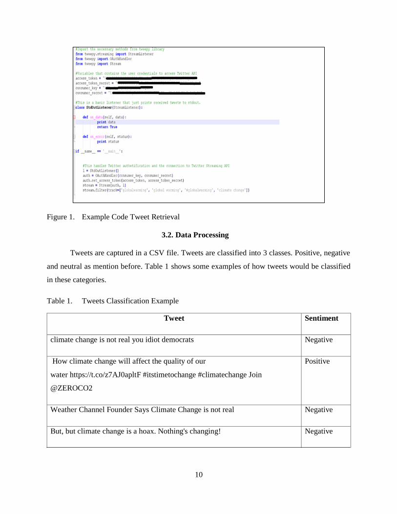
Tweets are captured in a CSV file. Tweets are classified into 3 classes. Positive, negative
and neutral as mention before. Table 1 shows some examples of how tweets would be classified
in these categories.
Table 1. Tweets Classification Example
Tweet Sentiment
climate change is not real you idiot democrats Negative
How climate change will affect the quality of our
water https://t.co/z7AJ0apltF #itstimetochange #climatechange Join
@ZEROCO2
Positive
Weather Channel Founder Says Climate Change is not real Negative
But, but climate change is a hoax. Nothing's changing! Negative
11
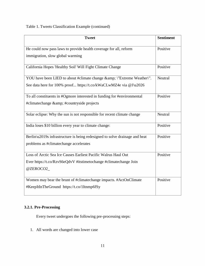
Table 1. Tweets Classification Example (continued)
Tweet Sentiment
He could now pass laws to provide health coverage for all, reform
immigration, slow global warming
Positive
California Hopes 'Healthy Soil' Will Fight Climate Change Positive
YOU have been LIED to about #climate change & \"Extreme Weather\".
See data here for 100% proof... https://t.co/kWaCLwMZ4e via @J\u2026
Neutral
To all constituents in #Ogmore interested in funding for #environmental
#climatechange & #countryside projects
Positive
Solar eclipse: Why the sun is not responsible for recent climate change Neutral
India loses $10 billion every year to climate change: Positive
Berlin\u2019s infrastructure is being redesigned to solve drainage and heat
problems as #climatechange accelerates
Positive
Loss of Arctic Sea Ice Causes Earliest Pacific Walrus Haul Out
Ever https://t.co/RzvS6eQdvV #itstimetochange #climatechange Join
@ZEROCO2_
Positive
Women may bear the brunt of #climatechange impacts. #ActOnClimate
#KeepItInTheGround https://t.co/1Itnmp6fSy
Positive
3.2.1. Pre-Processing
Every tweet undergoes the following pre-processing steps:
1. All words are changed into lower case
12
Ex: #Climate Change: The Challenge may be huge, but a Better World is 100%
POSSIBLE.
Outcome: climate change the challenge may be huge but a better world is 100% possible
2. http or https links are removed and replaced with LINK
Ex: Allowing #climatechange to continue is unfathomable. Here are some facts:
https://t.co/L0WW9xWT7K
Outcome: allowing climatechange to continue is unfathomable here are some facts LINK
3. @Usernames are removed and replaced with USER_REF
Ex: @LamarSmithTX21 Allowing #climatechange to continue is unfathomable. Here are
some facts https://t.co/L0WW9xWT7K
Outcome: USER_REF allowing climatechange to continue is unfathomable here are some
facts LINK
4. Removed all white spaces from tweets
Ex: @LamarSmithTX21 Allowing #climatechange to continue is unfathomable. Here are
some facts https://t.co/L0WW9xWT7K
Outcome: USER_REF allowing climatechange to continue is unfathomable here are some
facts LINK
5. Removed all hashtags from the tweets
Ex: Allowing #climatechange to continue is unfathomable. Here are some facts:
https://t.co/L0WW9xWT7K
Outcome: USER_REF allowing climatechange to continue is unfathomable here are some
facts LINK
6. Stripped all punctuations from the tweets
13
Ex: #ClimateChange: The Challenge may be huge, but a Better World is 100% POSSIBLE.
Outcome: Climatechange the challenge may be huge but a better world is possible.
Tweets were converted to lower case using python’s string class and lower() method. The
sub() method from python’s regular expression class was used to substitute URLs, usernames,
white spaces, hashtags with the relevant values as explained above. The strip() method from string
class is used to strip the remaining words of any punctuation.
3.2.2. Obtaining Stop Words List
Stop words are obtained from NLTK and Scikit libraries. I have also added USER_REF
and LINK to stop words list. To use custom stop words, all the stop words are listed one per line
in a text file. We read the file and each line in the file is appended to a stopwords list data structure
to be iterated over in later phases.
3.2.3. Stemming
Stemming is the process of identifying derived words and assigning a word to all the
derived words. This will reduce the size of index files. The initial tweet which is in the string
format is converted into a python list of substrings which can be used to obtain all the words and
punctuation in the tweet. The NLTK Tokenizer Package is used for this purpose. The initial string
is decoded to utf8 to avoid working on encoded strings. NLTK library already provides an
implementation of the porter stemmer algorithm in the nltk.stem.porter module. The tokenized
string is used as input to the porter stemmer.
Tokenizers divide strings into lists of substrings. For example, tokenizers can be used to
find the words and punctuation in a string:
Ex: A stemmer of the following words Beautiful, Beautifully, Beauty, Beauties can be
Beauty.
14
I have used Porter stemming algorithm for stemming the tweets. [32]
3.2.4. Big Picture
All the tweets are in a text file in the format of “sentiment, text”. We use python’s pandas
library (read_cvs method) (python data analysis library) to iterate over this file by mentioning the
separator as well as the file format. We use SCIKIT’s feature extraction module to extract features
from these text files. The count vectorizer method (feature_extraction.text. Count Vectorizer) is
used to convert these tweets into a matrix of token counts. This method uses the previously
described methods for preprocessing, tokenizing, stemming, stop word elimination, n-gram
generation, min_df selection to build the respective analyzers, preprocessors etc. The
tfidftransformer method in the same feature extraction module listed above operates on the count
matrix generated by count vectorizer to generate a normalized tf or tf-idf representation. The
classification algorithm works on this representation of the tweet along with the respective
sentiment to train the model.
15
4. TEST METHODOLOGY
The goal of this paper is to perform sentiment analysis on Global warming using twitter
data. I have used Naïve Bayes classifier, Multinomial Naïve Bayes Classifier and Support vector
machines combined with parameters like stop words, TF-IDF, N-gram. All classifiers are trained
with two datasets from twitter and accuracy test was performed on testing data set. Once the
algorithm is trained, to understand the perceptions of people over the years on global warming, I
have collected 5000 tweets each year for the past 10 years. After training the algorithms and
running through several optimization parameter tunings, the best classifier is used to work on the
historic climate change data to obtain the sentiment analysis.
4.1. Training Data
There are two datasets used in this study. The first is a 20K tweet dataset which is a
conglomerate of multiple publicly available datasets as pointed in [23, 24, 25]. Out of which 18K
are training tweets. The second is a 10K tweets climate change dataset, which I have captured from
twitter, processed and labeled sentiments. Out of which 8K comprise of the training set. The first
dataset comprises of general purpose labeled tweets whereas the second dataset is specific to tweets
related to global warming and climate change. Training data set is labeled with positive, negative
and neutral sentiments.
4.2. Testing Data
Once algorithms are trained on training set, test data set is used to perform experiments.
Both datasets mentioned in 4.1 have 2K testing and validation datasets.
4.3. Randomness
There is an aspect of randomness to the way training and test datasets are picked. For
instance, in the non-climate change dataset there are 18K tweets in the training set and 2K tweets
16
in the testing set. I used python’s random module to sample (random.sample(xrange(1, 20000),
18000) the required training dataset and the remaining 2k constitute the testing dataset. Each
iteration of the algorithm is trained over three randomly generated unique training and test datasets
sampled over the 20k tweets to obtain best performance. The same procedure is followed with
general purpose tweets as well as the climate change specific tweets.
17
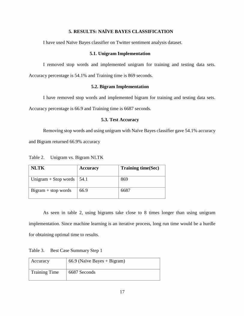
5. RESULTS: NAÏVE BAYES CLASSIFICATION
I have used Naïve Bayes classifier on Twitter sentiment analysis dataset.
5.1. Unigram Implementation
I removed stop words and implemented unigram for training and testing data sets.
Accuracy percentage is 54.1% and Training time is 869 seconds.
5.2. Bigram Implementation
I have removed stop words and implemented bigram for training and testing data sets.
Accuracy percentage is 66.9 and Training time is 6687 seconds.
5.3. Test Accuracy
Removing stop words and using unigram with Naïve Bayes classifier gave 54.1% accuracy
and Bigram returned 66.9% accuracy
Table 2. Unigram vs. Bigram NLTK
NLTK Accuracy Training time(Sec)
Unigram + Stop words 54.1 869
Bigram + stop words 66.9 6687
As seen in table 2, using bigrams take close to 8 times longer than using unigram
implementation. Since machine learning is an iterative process, long run time would be a hurdle
for obtaining optimal time to results.
Table 3. Best Case Summary Step 1
Accuracy 66.9 (Naïve Bayes + Bigram)
Training Time 6687 Seconds
18
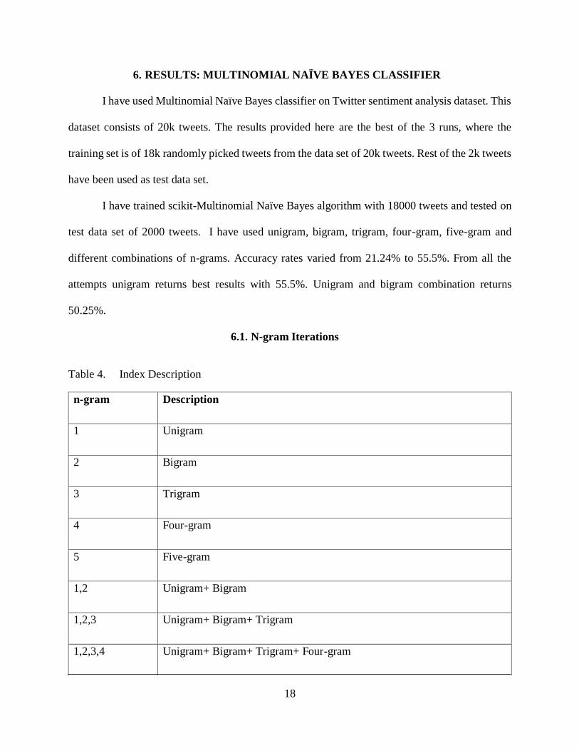
6. RESULTS: MULTINOMIAL NAÏVE BAYES CLASSIFIER
I have used Multinomial Naïve Bayes classifier on Twitter sentiment analysis dataset. This
dataset consists of 20k tweets. The results provided here are the best of the 3 runs, where the
training set is of 18k randomly picked tweets from the data set of 20k tweets. Rest of the 2k tweets
have been used as test data set.
I have trained scikit-Multinomial Naïve Bayes algorithm with 18000 tweets and tested on
test data set of 2000 tweets. I have used unigram, bigram, trigram, four-gram, five-gram and
different combinations of n-grams. Accuracy rates varied from 21.24% to 55.5%. From all the
attempts unigram returns best results with 55.5%. Unigram and bigram combination returns
50.25%.
6.1. N-gram Iterations
Table 4. Index Description
n-gram Description
1 Unigram
2 Bigram
3 Trigram
4 Four-gram
5 Five-gram
1,2 Unigram+ Bigram
1,2,3 Unigram+ Bigram+ Trigram
1,2,3,4 Unigram+ Bigram+ Trigram+ Four-gram
19
Table 4. Index Description (continued)
n-gram Description
1,2,3,4,5 Unigram+ Bigram+ Trigram+ Four-gram+ Five-gram
2,3,4,5 Bigram+ Trigram+ Four-gram+ Five-gram
3,4,5 Trigram+ Four-gram+ Five-gram
4,5 Four-gram+ Five-gram
Figure 2 below depicts the results from all selected combinations of multinomial Naïve
Bayes algorithm results using n-gram.
Figure 2. Impact of n-gram on Accuracy with Multinomial NB
Table 5. Best Case Summary Step 2
Accuracy 55.5%
Algorithm Multinomial Naïve Bayes + unigram
55.5 5245.25
31.421.24
50.25 47.6 45.7 44.2 47.2540.9
28.8
0102030405060
% a
ccura
cy
n-gram iteration
Impact of n-gram on accuracy
20
6.2. N-gram Iterations
Introducing smoothing factor α= 0.05 along with removing Stop words from training data
set returns 67.1% accuracy. I have taken a custom stop words list and also stop words list from
NLTK & Scikit corpus. In both the cases there is no difference in the results. In this test case,
unigram and bigram combination returned best results. Accuracy rate is 67.1% which is a huge
jump from the 55.5% in the previous test case. Figure 3 graph shows accuracy results of all selected
combinations using smoothing factor. Figure 3 points out that there is not much difference in
accuracy levels using either custom stop words or using the stop words from NLTK or SCIKIT
platforms.
Figure 3. Custom Stopwords vs. NLTK Corpus Stopwords
Table 6. Best Case Summary Step 3
Accuracy 66.7
Algorithm MNB+ Custom stop words, MNB+ stop words from NLTK & Scikit
64.9 66.7 67.1
21.5
64.9 66.7 67.1
21.5
0.0
10.0
20.0
30.0
40.0
50.0
60.0
70.0
80.0
1,2,3,4,5 1,2,3 1,2 5
%ac
cura
cy
n-gram iterations
Impact of Custom stopwords
Stopwords from scikit and nltk corpus Custom Stopword list
21
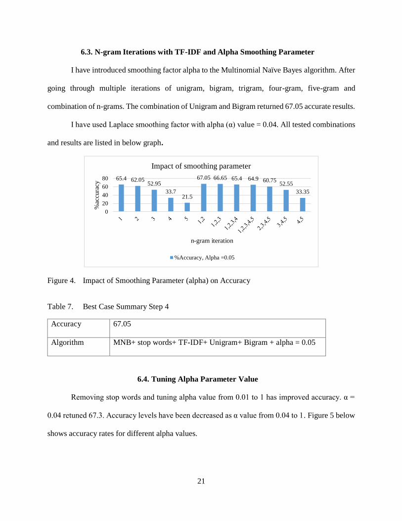
6.3. N-gram Iterations with TF-IDF and Alpha Smoothing Parameter
I have introduced smoothing factor alpha to the Multinomial Naïve Bayes algorithm. After
going through multiple iterations of unigram, bigram, trigram, four-gram, five-gram and
combination of n-grams. The combination of Unigram and Bigram returned 67.05 accurate results.
I have used Laplace smoothing factor with alpha (α) value = 0.04. All tested combinations
and results are listed in below graph.
Figure 4. Impact of Smoothing Parameter (alpha) on Accuracy
Table 7. Best Case Summary Step 4
Accuracy 67.05
Algorithm MNB+ stop words+ TF-IDF+ Unigram+ Bigram + alpha = 0.05
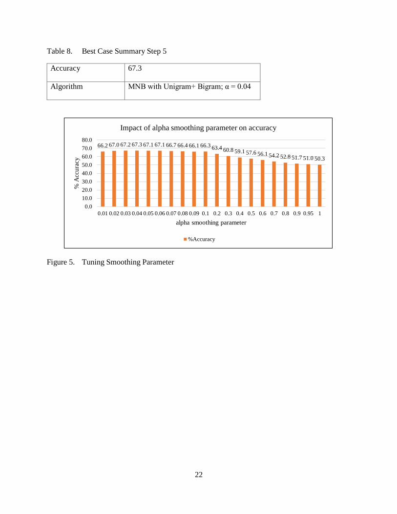
6.4. Tuning Alpha Parameter Value
Removing stop words and tuning alpha value from 0.01 to 1 has improved accuracy. α =
0.04 retuned 67.3. Accuracy levels have been decreased as α value from 0.04 to 1. Figure 5 below
shows accuracy rates for different alpha values.
65.4 62.0552.95
33.721.5
67.05 66.65 65.4 64.9 60.7552.55
33.35
0
20
40
60
80
%ac
cura
cy
n-gram iteration
Impact of smoothing parameter
%Accuracy, Alpha =0.05
22
Table 8. Best Case Summary Step 5
Accuracy 67.3
Algorithm MNB with Unigram+ Bigram; α = 0.04
Figure 5. Tuning Smoothing Parameter
66.2 67.0 67.2 67.3 67.1 67.1 66.7 66.4 66.1 66.3 63.4 60.8 59.1 57.6 56.1 54.2 52.8 51.7 51.0 50.3
0.0
10.0
20.0
30.0
40.0
50.0
60.0
70.0
80.0
0.01 0.02 0.03 0.04 0.05 0.06 0.07 0.08 0.09 0.1 0.2 0.3 0.4 0.5 0.6 0.7 0.8 0.9 0.95 1
% A
ccura
cy
alpha smoothing parameter
Impact of alpha smoothing parameter on accuracy
%Accuracy
23
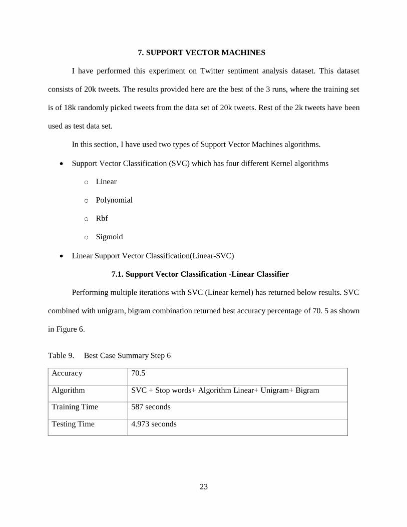
7. SUPPORT VECTOR MACHINES
I have performed this experiment on Twitter sentiment analysis dataset. This dataset
consists of 20k tweets. The results provided here are the best of the 3 runs, where the training set
is of 18k randomly picked tweets from the data set of 20k tweets. Rest of the 2k tweets have been
used as test data set.
In this section, I have used two types of Support Vector Machines algorithms.
Support Vector Classification (SVC) which has four different Kernel algorithms
o Linear
o Polynomial
o Rbf
o Sigmoid
Linear Support Vector Classification(Linear-SVC)
7.1. Support Vector Classification -Linear Classifier
Performing multiple iterations with SVC (Linear kernel) has returned below results. SVC
combined with unigram, bigram combination returned best accuracy percentage of 70. 5 as shown
in Figure 6.
Table 9. Best Case Summary Step 6
Accuracy 70.5
Algorithm SVC + Stop words+ Algorithm Linear+ Unigram+ Bigram
Training Time 587 seconds
Testing Time 4.973 seconds
24
Figure 6. Impact of N-gram on Accuracy with SVM-SVC-Linear kernel
As seen in Table 9, the run time here has reduced by more than 10x when compared to a
NLTK Naïve Bayes and bigram case as shown in Table 4. As Unigram and bigram combination
returned best results with Linear, So I have tried same combination with polynomial, sigmoid and
rbf algorithms. Results are listed in below table 10. The linear kernel still provides the best
performance compared to all the other kernels.
Table 10. Effect of Various Kernels in SVC on Accuracy
n-gram iteration Accuracy Kernels
1,2 16.6 poly
1,2 16.6 sigmoid
1,2 16.6 rbf
7.2. Linear Support Vector Classification
Linear SVM is similar to SVC with a linear kernel but Liner SVC is more flexible to
penalty and loss. It is also efficient with larger samples compared to SVC Linear as mentioned
68.95 62.7548.75
62.55
21.4
70.5 69.6 69.2 68.5 60.1545.15
30.25
020406080
% A
ccura
cy
n-gram iteration
SVM-SVC -Linear kernel
Accuracy
25
previously. Linear with Unigram and Bigram combination has returned best accuracy percentages
of 71%.
Table 11. Best Case Summary Step 7
Accuracy 71
Algorithm Linear SVC + Unigram+ Bigram
Training Time 0.387 Sec
Testing Time 0.003 Sec
Figure 7. Impact of N-gram on Linear SVC
As seen in Table 11. The time taken has reduced significantly compared to previously
tested use cases. After all the experiments, this is the best accuracy rate I have got. So, I have used
Linear SVC algorithm along with unigram and bigram combination on climate change data set.
7.3. Linear Support Vector Classification
I have performed this experiment on climate change dataset. This dataset consists of 10k
tweets. The results provided here are the best of the 3 runs, where the training set is of 8k randomly
picked tweets from the data set of 10k tweets. Rest of the 2k tweets have been used as test data set.
70.5563.9
50.75
32.8521.4
71 70.05 68.8 67.659.95
47.35
32.35
0
20
40
60
80
% A
ccura
cy
n-gram iteration
SVM-Linear SVC
Accuracy
26
I have used Linear SVC on Climate change data set. Linear SVC and unigram, bigram
combination returned 61.67%. From Figure 8, Table 11 and table 12, traditional datasets provide
better training accuracy compared to climate change specific datasets. This may be attributed to
the fact that a general twitter dataset from multiple sources will have more coverage in terms of
bag of words implementations compared to a specific climate change dataset where the algorithm
is limited to a smaller bag of words because of the scope of the smaller climate change dataset.
Figure 8. Using Climate Change Specific Dataset with Linear SVC
Table 12. Best Case Summary Step 8
Accuracy 61.76
Algorithm Linear SVC + (Unigram Bigram)
Training Time 0.144 Sec
Testing Time 0.001 Sec
61.28
59.6558.74
56.6255.37
61.76 61.3 61.43 61.5
59.79
58.21
56.38
52
54
56
58
60
62
64
% A
ccura
cy
n-gram iteration
Linear SVC- Climate change Dataset
Accuracy
27
8. SUMMARY OF TEST CASES
Naïve Bayes Classifier: I have experimented with Unigram and stop words, Bigram and
stop words. Unigram and stop words combination has returned best results in this case. In
Multinomial Naïve Bayes classifier, I have introduced smoothing parameter alpha, multiple n-
gram iterations with stop words has returned better accuracy results than Naïve Bayes classifier.
Using Multinomial Naïve Bayes classifier along with unigram, bigram combination, alpha value
as 0.04 has returned 67.3 % accuracy.
Support Vector Machines: I have used Support Vector Classification(SVC) algorithm and
Linear Support Vector Classification algorithms. After experimenting with multiple n-gram
iterations with different types of SVC algorithms and Linear SVC algorithm, Linear SVC has
returned best accuracy percentage with 71%.
Hence, the algorithm which will be used going forward to operate on historical climate
change dataset to understand year over year sentiments for global warming would be Linear SVC
as mentioned in Table 11.
28
9. TREND OF GLOBAL WARMING OVER THE YEARS
From all the tests, Linear SVC algorithm has given more accurate results. So, I have used
Linear SVC algorithm to find out year over year perceptions of global warming. I have collected
5000 tweets from each year and classified tweets using SVM- Linear SVC algorithm. Here are the
results.
Table 13. Global Warming Sentiment Analysis per year
2017 2016 2015 2014 2013 2012 2011 2010 2009 2008 2007
Positive 2655 2953 2635 3434 2631 2641 2943 2284 2265 637 32
Negative 2037 1777 2007 1129 2207 2157 1844 2383 2297 389 16
Neutral 310 273 359 435 170 199 218 331 437 4 0
Figure 9. Climate Change Trends over the Years
According to the data there are only 48 tweets related to Global warming in the year 2007.
Trend has started since then and the number of people tweeting about Global warming has
increased. Until 2010, the number of people who believed in global warming were almost
0
500
1000
1500
2000
2500
3000
3500
4000
2017 2016 2015 2014 2013 2012 2011 2010 2009 2008 2007
Climate change trends over the years
pos neg neutral

29
equivalent to the people who thought it was a hoax. Since 2011 trend has changed and more people
started believing in global warming.
30
10. CONCLUSION AND FUTURE WORK
The overall summary of this paper is listed in this section. The aim of this paper to perform
sentiment analysis of global warming using Twitter data worth of ten years. To achieve this, I
have used Naïve Bayes classifier, Multinomial Naïve Bayes Classifier and Support Vector
classification and Linear Support Vector classification algorithms to perform the classification
using n-gram iterations, TF-IDF and additive smoothing and removing stop words. Over all Linear
SVC with unigram, bigram combination has returned best accuracy with 71%. Hence, I have used
Linear SVC to analyze Global warming tweets worth of past 10 years. I have captured 5000 tweets
related to Global warming each year for past 10 years and used Linear SVC algorithm to analysis
the sentiment. Results returned that trend of tweeting about Global warming started increasing
since 2008. In 2009 and 2010 percentage of people used to think Global warming is real is almost
equal to number percentage of people think Global warming is a hoax. However, trend has
changed. In year 2014 percentage of positive tweets is way more than percentage of negative
tweets. When compared to 2014 percentages of positive tweets are higher than negative tweets but
percentage of positive tweets has started depreciating. Overall statistics says number of people
believe in Global warming are more than people who think Global warming is a hoax in the given
sample set.
Future work is to explore and venture into deep learning by evaluating Neural Networks
such as LSTM (Long Short-Term Memory) Networks for textual sentiment analysis.
31
REFERENCES
1. Earth Science Communication Team, NASA, Global Climate Change Vital Signs of the Planet
https://climate.nasa.gov/effects/
Retrieved on 07/21/2017
2. Melissa Denchak , March 2016, Are the Effects of Global Warming really that Bad
https://www.nrdc.org/stories/are-effects-global-warming-really-bad
Retrieved on 07/21/2017
3. Union of Concerned Scientists, Global Warming Impacts
http://www.ucsusa.org/our-work/global-warming/science-and-impacts/global-warming-
impacts#.WhjTd0qnHIU
Retrieved on 07/21/2017
4. Joshua Roesslein, Tweepy Documentation
http://tweepy.readthedocs.io/en/v3.5.0/
Retrieved on 07/19/2017
5. NLTK 3.2.5 Documentation,
http://www.nltk.org/_modules/nltk/classify/naivebayes.html
Retrieved on 08/02/2017
6. Adil Moujahid, July 2014, An Introduction to Text Mining using Twitter Streaming API and
Python
http://adilmoujahid.com/posts/2014/07/twitter-analytics/
Retrieved on 07/19/2017
7. http://www.tfidf.com/
Retrieved on 08/28/2017
8. Mike Waldron, June 2015, Naïve Bayes for Dummies, A Simple Explanation
http://blog.aylien.com/naive-bayes-for-dummies-a-simple-explanation/
Retrieved on 07/30/2017
9. Hatem Faheem, July 2015, How are N-grams Used in Machine Learning
https://www.quora.com/How-are-N-grams-used-in-machine-learning
Retrieved on 08/01/2017
32
10. Why is N-gram Used in Text Language Identification Instead of Words
https://stats.stackexchange.com/questions/144900/why-is-n-gram-used-in-text-language-
identification-instead-of-words
Retrieved on 08/01/2017
11. Abinash Tripaty, Ankit Agarwal, Santanu Kumar Rath, March 2016, Classification of
Sentiment Reviews using N-gram Machine Learning Approach
http://www.sciencedirect.com/science/article/pii/S095741741630118X
Retrieved on 07/21/2017
12. Johannes Furnkranz, A Study Using n-gram Features for Text Categorization
http://citeseerx.ist.psu.edu/viewdoc/download?doi=10.1.1.49.133&rep=rep1&type=pdf
Retrieved on 08/20/2017
13. Manoj Bisht, July 2016, Document Classification using Multinomial Naïve Bayes Classifier
https://www.3pillarglobal.com/insights/document-classification-using-multinomial-naive-
bayes-classifier
Retrieved on 09/21/2017
14. Difference between Naïve Bayes and Multinomial Naïve Bayes
https://stats.stackexchange.com/questions/33185/difference-between-naive-bayes-
multinomial-naive-bayes
Retrieved on 09/21/2017
15. Difference between Naïve Bayes and Multinomial Naïve Bayes
https://stats.stackexchange.com/questions/33185/difference-between-naive-bayes-
multinomial-naive-bayes
Retrieved on 09/21/2017
16. Chistopher D. Manning, Prabhakar Raghavan, Hinrich Schutze, April 2009, Naïve Bayes Text
Classification
https://nlp.stanford.edu/IR-book/html/htmledition/naive-bayes-text-classification-1.html
Retrieved on 07/20/2017
17. Multinomial Naïve Bayes Classifier
http://scikitlearn.org/stable/modules/generated/sklearn.naive_bayes.MultinomialNB.html#skl
earn.naive_bayes.MultinomialNB
Retrieved on 09/25/2017
33
18. Introduction to Support Vector Machines
http://docs.opencv.org/2.4/doc/tutorials/ml/introduction_to_svm/introduction_to_svm.html
Retrieved on 09/25/2017
19. Jacob Perkins, May 2010, Text Classification for Sentiment Analysis-Naïve Bayes Classifier
https://streamhacker.com/2010/05/10/text-classification-sentiment-analysis-naive-bayes-
classifier/
Retrieved on 08/20/2017
20. Sunil Ray, September 2017, Understanding Support Vector Machine Algorithm from
Examples
https://www.analyticsvidhya.com/blog/2017/09/understaing-support-vector-machine-
example-code/
Retrieved on 09/26/2017
21. Sunil Ray, September 2017, 6 Easy Steps to Learn Naïve Bayes Algorithm
https://www.analyticsvidhya.com/blog/2017/09/naive-bayes-explained/
Retrieved on 08/20/2017
22. A Beginner’s Guide to Recurrent Networks and LSTMs
https://deeplearning4j.org/lstm.html
Retrieved on 08/25/2017
23. Nick Diakopoulos and Shamma, D.A, 2008 US Election debate, Twitter sentiment dataset -
Retrieved on 07/20/2017
24. Niek Sanders, Twitter sentiment corpus
Retrieved on 07/25/2017
25. A lot of sentiment datasets via CS Dept, Cornell University
Retrieved on 07/27/2017
26. Tweepy/Examples/ streaming.py
https://github.com/tweepy/tweepy/blob/master/examples/streaming.py
Retrieved on 07/27/2017
27. Rahul Saxena, February 2017, How the Naïve Bayes Classifier Works in Machine Learning,
http://dataaspirant.com/2017/02/06/naive-bayes-classifier-machine-learning/
Retrieved on 07/22/2017
34
28. Scikit learn- Support Vector Machines
http://scikit-learn.org/stable/modules/svm.html
Retrieved on 09/20/2017
29. Jacob Perkins, May 2010, Text Classification for Sentiment analysis- Stopwords and
Collocations,
https://streamhacker.com/2010/05/24/text-classification-sentiment-analysis-stopwords-
collocations/
Retrieved on 09/05/2017
30. Scikit learn- sklearn.naive_bayes.MultinomialNB
http://scikit-learn.org/stable/modules/generated/sklearn.naive_bayes.
MultinomialNB.html
Retrieved on 08/20/2017
31. Ravikiran Janardhana, May 2012, How to Build a Twitter Sentiment Analyzer
https://www.ravikiranj.net/posts/2012/code/how-build-twitter-sentiment-analyzer/
Retrieved on 08/15 /2017
32. Martin Porter, January 2006, The Porter Stemming Algorithm,
https://tartarus.org/martin/PorterStemmer/
Retrieved on 08/20 /2017