Embed Size (px)
Citation preview
SEP Manual
Robert G. Clapp, Marie L. Prucha, Paul Sava, Joe Dellinger, Biondo Biondi
c© February 11, 2004

Contents
1 SEPlib 1
1.1 What’s Here? . . . . . . . . . . . . . . . . . . . . . . . . . . . . . . . . . . 1
1.2 Overview - using SEPlib . . . . . . . . . . . . . . . . . . . . . . . . . . . . 1
1.2.1 Getting the test data . . . . . . . . . . . . . . . . . . . . . . . . . . 2
1.2.2 History files . . . . . . . . . . . . . . . . . . . . . . . . . . . . . . . 4
1.2.3 The SEPlib datacube . . . . . . . . . . . . . . . . . . . . . . . . . . 7
1.3 Illustrative examples . . . . . . . . . . . . . . . . . . . . . . . . . . . . . . 8
1.3.1 Playing with parameters . . . . . . . . . . . . . . . . . . . . . . . . 8
1.3.2 Parameters, parameter files, and history files . . . . . . . . . . . . . . 11
2 SEP3D Introduction 13
2.1 SEP3D Overview . . . . . . . . . . . . . . . . . . . . . . . . . . . . . . . . 13
2.2 Data Format . . . . . . . . . . . . . . . . . . . . . . . . . . . . . . . . . . . 14
2.2.1 Structure of a SEP3D data set . . . . . . . . . . . . . . . . . . . . . 14
2.2.2 Data and Headers Coordinate System . . . . . . . . . . . . . . . . . 15
2.2.3 Mapping between the header records and the data records . . . . . . 15
2.2.4 Gridding information . . . . . . . . . . . . . . . . . . . . . . . . . . 16
2.3 SEP3D Standards . . . . . . . . . . . . . . . . . . . . . . . . . . . . . . . . 17
2.3.1 Standard header names . . . . . . . . . . . . . . . . . . . . . . . . . 17
2.4 Superset . . . . . . . . . . . . . . . . . . . . . . . . . . . . . . . . . . . . . 17
3 Programs 21
3.1 SEPlib programs . . . . . . . . . . . . . . . . . . . . . . . . . . . . . . . . 21
CONTENTS
3.1.1 Useful non-SEPlib programs . . . . . . . . . . . . . . . . . . . . . . 30
3.2 SEP3D programs . . . . . . . . . . . . . . . . . . . . . . . . . . . . . . . . 31
3.3 Graphics programs . . . . . . . . . . . . . . . . . . . . . . . . . . . . . . . 32
3.4 Converters . . . . . . . . . . . . . . . . . . . . . . . . . . . . . . . . . . . . 34
3.4.1 SEG-Y and SU converters . . . . . . . . . . . . . . . . . . . . . . . 34
3.4.2 Vplot converters . . . . . . . . . . . . . . . . . . . . . . . . . . . . 34
4 Ricksep 37
4.1 Ricksep documentation . . . . . . . . . . . . . . . . . . . . . . . . . . . . . 37
4.2 Examples . . . . . . . . . . . . . . . . . . . . . . . . . . . . . . . . . . . . 45
5 Example flows 49
5.1 Regular Datasets . . . . . . . . . . . . . . . . . . . . . . . . . . . . . . . . 49
5.1.1 Creating synthetics . . . . . . . . . . . . . . . . . . . . . . . . . . . 49
5.1.2 Creating velocity models . . . . . . . . . . . . . . . . . . . . . . . . 50
5.1.3 Wave equation modeling . . . . . . . . . . . . . . . . . . . . . . . . 50
5.1.4 NMO/Muting/Velocity analysis . . . . . . . . . . . . . . . . . . . . 53
5.2 SEP3D Datasets . . . . . . . . . . . . . . . . . . . . . . . . . . . . . . . . . 55
5.2.1 Reading from SEGY . . . . . . . . . . . . . . . . . . . . . . . . . . 57
5.2.2 Viewing and manipulating headers . . . . . . . . . . . . . . . . . . . 57
5.2.3 Sorting and binning . . . . . . . . . . . . . . . . . . . . . . . . . . . 61
5.2.4 Reading and writing to SEGY/SU . . . . . . . . . . . . . . . . . . . 62
5.2.5 Velocity analysis/NMO . . . . . . . . . . . . . . . . . . . . . . . . . 62
5.2.6 Creating synthetics . . . . . . . . . . . . . . . . . . . . . . . . . . . 63
5.3 Travel times . . . . . . . . . . . . . . . . . . . . . . . . . . . . . . . . . . . 63
5.4 PEFs . . . . . . . . . . . . . . . . . . . . . . . . . . . . . . . . . . . . . . . 65
5.4.1 Texture synthesizing and seismic decon with prediction-error filters . 66
6 Tricky things 75
6.1 Piping in SEP3d . . . . . . . . . . . . . . . . . . . . . . . . . . . . . . . . . 75
6.2 Handling large files . . . . . . . . . . . . . . . . . . . . . . . . . . . . . . . 75
CONTENTS
6.3 Fancy plotting . . . . . . . . . . . . . . . . . . . . . . . . . . . . . . . . . . 76
6.3.1 Advanced plotting . . . . . . . . . . . . . . . . . . . . . . . . . . . 76
6.3.2 Plot matrices . . . . . . . . . . . . . . . . . . . . . . . . . . . . . . 77
6.4 Headermapping on the fly . . . . . . . . . . . . . . . . . . . . . . . . . . . . 78
6.5 SU support . . . . . . . . . . . . . . . . . . . . . . . . . . . . . . . . . . . 79
6.5.1 Example . . . . . . . . . . . . . . . . . . . . . . . . . . . . . . . . 80
7 Makerules 81
7.1 Compile Rules . . . . . . . . . . . . . . . . . . . . . . . . . . . . . . . . . 81
7.2 Example and translation . . . . . . . . . . . . . . . . . . . . . . . . . . . . 83
7.2.1 Example Makefile . . . . . . . . . . . . . . . . . . . . . . . . . . . 83
7.2.2 Translation . . . . . . . . . . . . . . . . . . . . . . . . . . . . . . . 84
8 Libraries 85
8.1 Summary of libraries . . . . . . . . . . . . . . . . . . . . . . . . . . . . . . 85
8.2 Library: sep . . . . . . . . . . . . . . . . . . . . . . . . . . . . . . . . . . . 86
8.3 Library: sep3d . . . . . . . . . . . . . . . . . . . . . . . . . . . . . . . . . . 87
8.4 Library: sep2df90 . . . . . . . . . . . . . . . . . . . . . . . . . . . . . . . . 89
8.5 Library: supersetf90 . . . . . . . . . . . . . . . . . . . . . . . . . . . . . . . 89
8.6 Library: sepaux . . . . . . . . . . . . . . . . . . . . . . . . . . . . . . . . . 90
8.7 Library: sepauxf90 . . . . . . . . . . . . . . . . . . . . . . . . . . . . . . . 90
8.8 Library: geef90 . . . . . . . . . . . . . . . . . . . . . . . . . . . . . . . . . 90
8.9 Library: sepfilter . . . . . . . . . . . . . . . . . . . . . . . . . . . . . . . . 93
8.10 Library: sepfilterf90 . . . . . . . . . . . . . . . . . . . . . . . . . . . . . . . 93
8.11 Library: sepfft . . . . . . . . . . . . . . . . . . . . . . . . . . . . . . . . . . 94
8.12 Library: septravel . . . . . . . . . . . . . . . . . . . . . . . . . . . . . . . . 94
8.13 Library: sepvelanf . . . . . . . . . . . . . . . . . . . . . . . . . . . . . . . . 94
8.14 Library: sepvelanf90 . . . . . . . . . . . . . . . . . . . . . . . . . . . . . . 94
8.15 Library: sepmath . . . . . . . . . . . . . . . . . . . . . . . . . . . . . . . . 95
8.16 Library: sepmathf90 . . . . . . . . . . . . . . . . . . . . . . . . . . . . . . 95
CONTENTS
8.17 Library: sepsu . . . . . . . . . . . . . . . . . . . . . . . . . . . . . . . . . . 96
8.18 Library: oclib . . . . . . . . . . . . . . . . . . . . . . . . . . . . . . . . . . 96
8.18.1 Summary of oclib . . . . . . . . . . . . . . . . . . . . . . . . . . . 96
8.18.2 oclib . . . . . . . . . . . . . . . . . . . . . . . . . . . . . . . . . . 97
9 Writing a program 117
9.1 How to write a SEPlib program . . . . . . . . . . . . . . . . . . . . . . . . . 117
9.1.1 Language: C . . . . . . . . . . . . . . . . . . . . . . . . . . . . . . 117
9.1.2 Language: Fortran77 . . . . . . . . . . . . . . . . . . . . . . . . . . 119
9.1.3 Language: Ratfor . . . . . . . . . . . . . . . . . . . . . . . . . . . . 121
9.1.4 Language: Fortran90 . . . . . . . . . . . . . . . . . . . . . . . . . . 123
9.1.5 Language: Ratfor90 . . . . . . . . . . . . . . . . . . . . . . . . . . 125
9.1.6 Language: C calling Fortran . . . . . . . . . . . . . . . . . . . . . . 126
9.1.7 Language: Fortran calling C . . . . . . . . . . . . . . . . . . . . . . 129
9.2 How to write a SEP3D program . . . . . . . . . . . . . . . . . . . . . . . . 131
9.2.1 SEP3D . . . . . . . . . . . . . . . . . . . . . . . . . . . . . . . . . 131
9.2.2 Superset . . . . . . . . . . . . . . . . . . . . . . . . . . . . . . . . . 138
9.3 How to write a vplot program . . . . . . . . . . . . . . . . . . . . . . . . . . 143
9.4 Writing in SEP’s Fortran90 inversion library . . . . . . . . . . . . . . . . . . 144
9.4.1 Out-of-core . . . . . . . . . . . . . . . . . . . . . . . . . . . . . . . 144
9.4.2 In-core . . . . . . . . . . . . . . . . . . . . . . . . . . . . . . . . . 146
9.5 How to use MPI . . . . . . . . . . . . . . . . . . . . . . . . . . . . . . . . . 148
9.5.1 Makefile . . . . . . . . . . . . . . . . . . . . . . . . . . . . . . . . 148
9.5.2 MPI program . . . . . . . . . . . . . . . . . . . . . . . . . . . . . . 148
10 Preprocessors 151
10.1 Introduction . . . . . . . . . . . . . . . . . . . . . . . . . . . . . . . . . . . 151
10.2 Ratfor basics . . . . . . . . . . . . . . . . . . . . . . . . . . . . . . . . . . 151
10.3 Changes from Ratfor77 . . . . . . . . . . . . . . . . . . . . . . . . . . . . . 152
10.3.1 Backward compatibility issues . . . . . . . . . . . . . . . . . . . . . 152
CONTENTS
10.3.2 Extensions . . . . . . . . . . . . . . . . . . . . . . . . . . . . . . . 153
10.4 SEP extensions . . . . . . . . . . . . . . . . . . . . . . . . . . . . . . . . . 153
10.4.1 Memory allocation . . . . . . . . . . . . . . . . . . . . . . . . . . . 153
10.4.2 Parameter handling . . . . . . . . . . . . . . . . . . . . . . . . . . . 154
10.4.3 Ratfor90 code . . . . . . . . . . . . . . . . . . . . . . . . . . . . . . 155
10.4.4 Translated Fortran90 Code . . . . . . . . . . . . . . . . . . . . . . . 155
10.5 Downloading/installing . . . . . . . . . . . . . . . . . . . . . . . . . . . . . 158
10.6 Error handling . . . . . . . . . . . . . . . . . . . . . . . . . . . . . . . . . . 159
11 SEPlib outside SEP 161
11.1 Installing SEPlib . . . . . . . . . . . . . . . . . . . . . . . . . . . . . . . . 161
11.2 How to modify and compile SEPlib . . . . . . . . . . . . . . . . . . . . . . 163
11.3 Setting up the SEP environment . . . . . . . . . . . . . . . . . . . . . . . . 163
11.4 How to compile and run SEP reports remotely . . . . . . . . . . . . . . . . . 164
11.5 Converting old versions of SEPlib . . . . . . . . . . . . . . . . . . . . . . . 165
11.6 Basic Troubleshooting . . . . . . . . . . . . . . . . . . . . . . . . . . . . . 165
11.6.1 More specific problems . . . . . . . . . . . . . . . . . . . . . . . . . 166
11.7 Important Contributors . . . . . . . . . . . . . . . . . . . . . . . . . . . . . 166

CONTENTS
Chapter 1
SEPlib
SEPlib is a software package developed by members of the Stanford Exploration Project. Itcontains programs to manipulate and process many types of geophysical data. SEP studentsmay view this manual in DVI form by typing SEPMAN in any shell.
1.1 What’s Here?
1.2 Overview - using SEPlib
Although SEPlib currently consists of over 100 different programs, they share many commonfeatures. First of all, by convention SEPlib programs start with a Capital Letter. More impor-tantly, most SEPlib programs are “filters”; they read from standard input and write to standardoutput:
Prog < input > output
Complex functions are created by joining filters with pipes:
Prog1 < in | Prog2 | Prog3 > out
We will use the SEPlib program Wiggle to demonstrate some basic SEPlib-program properties.Wiggle is just a simple program that converts raw data into wiggle traces, but it is used a lotbecause people are usually curious to see what they have done to their data.
Try typing:
Wiggle
1
2 CHAPTER 1. SEPLIB
You should get a couple of screens’ worth of documentation. This is called self documentation:run the program without arguments, input, or output, and it will display a brief documentationsummary. Almost all SEPlib programs will self document, which is good because very few ofthem have real manual pages.
If you get an error message doc(): No such file or directory, complain to the personwho installed SEPlib at your site! If you don’t feel like complaining (perhaps because you arethat person) and you know where the SEPlib source is installed, you can tell SEPlib programsan alternate place to look for their source by setting the environment variable SEP_DOC_PATH.See the “SEPlib Outside SEP” chapter.
1.2.1 Getting the test data
Hopefully you have now worked out any software-environment problems you might have hadbefore, and you are ready for your “test drive”.
There should be three data files in the directory where you found this paper. Txx.HH,Txy.HH and Txz.HH. Plot one of these files by doing
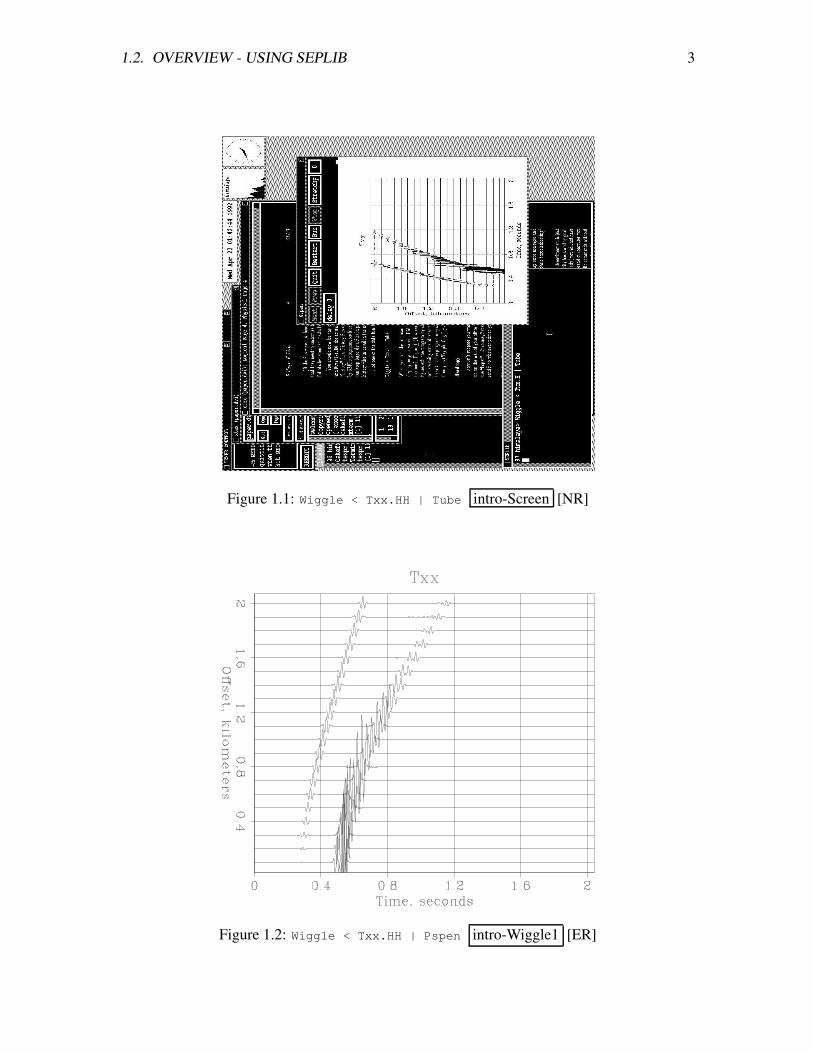
Wiggle < Txx.HH | Tube
When you run the command above Wiggle creates a plot which Tube then tries to display onyour screen. Did it work? Hopefully your screen will look something like the one in Figure ??.(If when you try it “Tube” does the plot using the graphics device Xtpen, like in the figure, exitthe program by clicking on the QUIT button at the top of the window. If you are using someother sort of graphics device you may have to hit return or space to exit, or the program maysimply exit when the plot is done without any prompting from you.) Try displaying Txy.H andTxz.H too.
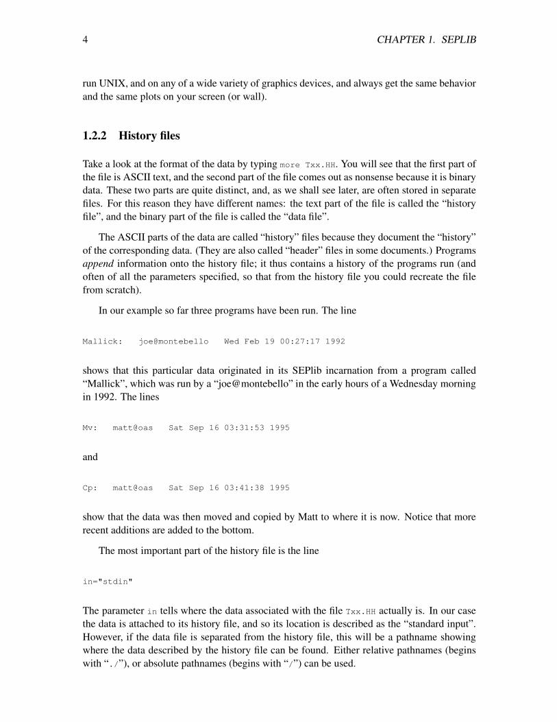
Now we can try printing the plot using Pspen. Of course, Pspen has to know where tosend the plot. By default it will send it to whatever printer your local machine thinks is called“postscript”. Try:
Wiggle < Txx.HH | Pspen
Hopefully this will work, producing something like Figure 1.2. If the printer your workstationcalls “postscript” turns out to be old and slow, on another floor or in another building, or youoften get strange error messages and partial plots when you attempt to plot big files, check the“Tricky Things” chapter for some advice.
At this point you may be thinking that setting up your SEPlib environment is just tootedious to be worth it. Don’t despair; the apparent complexity has a worthy goal. The idea ofSEPlib and “Tube” is that (if things are set up correctly) you will not have to worry about whatdevice you are sitting at or even what brand of computer you are logged into. You should beable to just use the same SEPlib commands without worry on any of your local computers that
1.2. OVERVIEW - USING SEPLIB 3
Figure 1.1: Wiggle < Txx.HH | Tube intro-Screen [NR]
Figure 1.2: Wiggle < Txx.HH | Pspen intro-Wiggle1 [ER]
4 CHAPTER 1. SEPLIB
run UNIX, and on any of a wide variety of graphics devices, and always get the same behaviorand the same plots on your screen (or wall).
1.2.2 History files
Take a look at the format of the data by typing more Txx.HH. You will see that the first part ofthe file is ASCII text, and the second part of the file comes out as nonsense because it is binarydata. These two parts are quite distinct, and, as we shall see later, are often stored in separatefiles. For this reason they have different names: the text part of the file is called the “historyfile”, and the binary part of the file is called the “data file”.
The ASCII parts of the data are called “history” files because they document the “history”of the corresponding data. (They are also called “header” files in some documents.) Programsappend information onto the history file; it thus contains a history of the programs run (andoften of all the parameters specified, so that from the history file you could recreate the filefrom scratch).
In our example so far three programs have been run. The line
Mallick: joe@montebello Wed Feb 19 00:27:17 1992
shows that this particular data originated in its SEPlib incarnation from a program called“Mallick”, which was run by a “joe@montebello” in the early hours of a Wednesday morningin 1992. The lines
Mv: matt@oas Sat Sep 16 03:31:53 1995
and
Cp: matt@oas Sat Sep 16 03:41:38 1995
show that the data was then moved and copied by Matt to where it is now. Notice that morerecent additions are added to the bottom.
The most important part of the history file is the line
in="stdin"
The parameter in tells where the data associated with the file Txx.HH actually is. In our casethe data is attached to its history file, and so its location is described as the “standard input”.However, if the data file is separated from the history file, this will be a pathname showingwhere the data described by the history file can be found. Either relative pathnames (beginswith “./”), or absolute pathnames (begins with “/”) can be used.
1.2. OVERVIEW - USING SEPLIB 5
The rest of the file gives other important information:esize=4 indicates the data consists of elements 4 bytes long;data_format="xdr_float" indicates these 4-byte long elements are in fact machine-independentIEEE floating-point numbers.n1=1024 n2=20 indicates the data is in a 2-dimensional array with a fast axis 1024 elementslong and a slow axis 20 elements long.o1=0 d1=.002 label1="Time, seconds" indicates the fast axis has dimensions of seconds,with the first element corresponding to time 0, the second element time .002, the third .004,etc.o2=.1 d2=.1 label2="Offset, kilometers" indicates the slow axis has dimensions of kilo-meters, with the first element corresponding to an offset of .1 kilometers, the second element.2, the third .3, etc.
So far we have displayed our data without creating any new files at all. We did this byusing UNIX pipelines (“|”). These tell the operating system we want to pass the information(both data and parameters) from one program to another, and we don’t want to be botheredwith having to keep track of any temporary intermediate files ourselves.
We could have done it differently by saving the output of the programs. Let’s see how ourfavorite example
Wiggle < Txx.HH | Tube
can be split up into two separate steps1:
Wiggle < Txx.HH > Out.H
Tube < Out.H
where Out.H is the output of Wiggle.2 (Type “man vplot” if you are curious what sort of outputWiggle writes.)
Take a look at the the output file with more Out.H. This time you will only see the ASCIIhistory file. So the question is: where has the actual data gone? This might be interesting ifyou are playing around with files of a size of several 100MBytes, given that we all have toface the fact that free diskspace is always limited.
Unless otherwise instructed, SEPlib will attempt to separate your data files from your his-tory files. The advantage of this is that you may want to keep large, bulky data files somewhereaway from your home directory, where you do most of your work.
There are four options for directing your output:
By default SEPlib will attempt to put the raw data in a subdirectory with your usernameunder the system-default SEPlib “scratch” directory. If you tried the commands above and got
1the fact that the original data has the suffix HH and the output only has a single H is nothing to do withSEPlib - it just stops the original data from being deleted when the directory is cleaned, with gmake clean
for example2If you just got an error message don’t panic yet, just keep reading.
6 CHAPTER 1. SEPLIB
an error message something likeoutput(): No such file or directory This means your default directory did not exist.Look to see what directory Wiggle was trying to use, and create it if you wish (and havesufficient permissions to do so) using the UNIX command “mkdir”; then try our exampleagain. Be warned that to keep such “public” data areas from filling with junk, they are usuallysubject to swift and merciless disk mowing.
Alternatively, you can specify where you want the data files to go with a command-lineparameter, for example:
Wiggle < Txx.HH > Out.H out=./Data/Out.datafile
but it might get tiring to do this every single time! (For a quick experiment you might want totry the above example with and without the leading “./” in the out= argument, and note whatin= gets set to in Out.H in each case. Unless the SEPlib output subroutine sees a leading “./”,it automatically expands output file names to fully qualified paths.)
Another, better, solution is for you to create a personal directory to keep your data insomewhere, and tell SEPlib that’s where you want it to put your data by default. Let’s supposeyou create a directory called “Data” under your home directory. You then tell SEPlib to putdata files there by doing:
setenv DATAPATH ~/Data/
(Note in this example the leading ~ will get expanded to your full home directory name by thecsh before the DATAPATH variable is set.) Remember that binary data files will accumulatein the directory given by your DATAPATH if you are not careful. Make sure to use Rm, notrm, to delete SEPlib files! (Examples of using Rm to remove SEPlib files can be found laterin this document.)
Note that the DATAPATH is simply prepended as an arbitrary string to a slightly modifiedversion of the history filename to get a name for the data file, so you probably want yourDATAPATH to end with a “/”, like the example above does. You can also set your datapath bycreating a file called “.datapath” in your home directory (or in your current directory, withthe one in your current directory taking precedence). The .datapath file should contain a linelooking something like
datapath=/net/kana/joe/Data/
Note in the file you have to expand out your full home-directory name yourself. This willcause the binary file to always be written to your home directory on kana. If you are workingon a different machine (let’s say you are working on redbluff) and want to write to a scratchdrive on that machine, you can put a line like this in your .datapath file:
redbluff datapath=/net/redbluff/scr1/joe/
1.2. OVERVIEW - USING SEPLIB 7
Finally, if you want the data to stay attached to the history file you can use the out=
command line option again but this time send the data to the standard output along with thehistory file:
Wiggle < Txx.HH > Out.H out="stdout"
1.2.3 The SEPlib datacube
If we have data frames of the same size (like shot records usually are) we can easily mergethem into a “datacube” to make their processing easier. Let’s try to merge the three filesTxx.HH Txy.HH and Txz.HH into a datacube using the program “Cat”, which does to SEPlibfiles something like what “cat” does to ASCII files.
Cat Txx.HH Txy.HH Txz.HH > Three.H
Now make a wiggle plot of this new file by doing:
Wiggle < Three.H | Tube
/par Pretty snazzy, eh? Tube realizes that there are three different panels, so it shows all threeof them.3
Look at the history file Three.H to see how history “accumulated” in this example. Ingeneral, each successive SEPlib program writes more information onto the end of the historyfile. (Cat is a bit of a special case, since it is always called with multiple input files and doesn’tuse redirected input. Most SEPlib programs read a file from standard input and write a fileto standard output. The SEPlib input and output subroutines shared by all such “standard”programs begin by automatically copying the input header straight across to the output un-changed. Anything the running program wants to add to the history then gets appended. Cathas to do the copying “by hand”, so its output looks a little different.)
Note that lines setting parameters such as “n3=1” can occur multiple times in one historyfile, as various programs set old parameters to new values. The last-defined value is the onlyvalid one, because it is the “most recent” and corresponds to the current data.
You might be thinking now that using “more” to examine history files to find the dimen-sions of the associated data file can get confusing and tedious if the history is long and com-plex. A quick way to examine the dimensions and properties of a SEPlib file is to use thecommand “In”:
3Hardcopy devices will print out three separate pages of plots. On devices where you can see either thetext screen or the graphics screen (but not both at the same time) you may have to hit “Return” to workthrough the sequence of plots one at a time. On most other screen devices the three plots will simply zip byin quick succession; you have to give an option to tell it to slow down or wait for a keypress. If your penprogram is Xtpen it will animate the three frames for you, Movie-style.
8 CHAPTER 1. SEPLIB
In Three.H
gives the salient features of the dataset
Three.H:
in="/usr/local/sep/scr/joe/Three.H@"
expands to in="/usr/local/sep/scr/joe/Three.H@"
esize=4
n1=1024 n2=20 n3=3 61440 elem 245760 bytes
d1=.002 d2=.1 d3=1
o1=0 o2=.1 o3=0
label1=Time, seconds
label2=Offset, kilometers
Note that “Three.H” is a three-dimensional block of data, with n3=3.
When you are done with Three.H, delete it by doing
Rm Three.H
This will delete both the history file and its associated binary data file. If you slip and acciden-tally use rm instead, the binary data file will remain behind uselessly cluttering up your datadirectory, possibly forever if nothing ever looks for junk files to clean up there.
Warning: the default behavior of both rm and Rm is to go ahead and delete without con-firmation. You probably have rm aliased to rm -i (you may have forgotten doing it), but youprobably don’t have Rm aliased to Rm -i. You may want to do that now.
1.3 Illustrative examples
1.3.1 Playing with parameters
SEPlib programs generally do simple things. They are still very flexible, though, becausetheir default behavior can be modified by appropriate command-line or history-file parameters.Most programs have at least a few options or parameters; some of them have hundreds. Let’slook at some relatively simple examples.
We saw already that most of the Txx.HH data consists of zero values that are not veryinteresting for us. Let’s trim the data a bit. The SEPlib utility Window is used for this purpose.If you remember, Txx.HH consists of 1 plane of 20 traces, with 1024 samples in each trace.4
In SEPlib notation, n3=1 n2=20 n1=1024. Let’s “zoom in” on the interesting part of thedata between times .4 and .8 seconds and offsets from the smallest (.1) up to 1. (i.e., we will
4If not, you can always check by running In Txx.HH!
1.3. ILLUSTRATIVE EXAMPLES 9
keep samples 200 through 400 of the first 10 traces). To do its job Window needs to know thenumber of samples and the first sample to accept for each axis. (The defaults are “all of themthat you can” and “begin at the beginning”, respectively.) For our example we would have:
Window < Txx.HH n2=10 n1=200 f1=200 > Txx_Windowed.H
Fortunately Window is smart enough to understand your command using the values on the twoaxes too:
Window < Txx.HH min1=.4 max1=.8 max2=1. > Txx_Windowed.H
We must warn you that the second method is more risky, since it is possible that you have anerror in the sampling parameters such as o1 and d1 in the history file, or you simply forgot tospecify them at all (so they defaulted to 0 and 1 respectively). You may prefer to tell Windowwhere to start and end using integer sample numbers. If you are sure that you would nevermake such mistakes, did you catch the discrepancy in the two examples above? You’ll findthey don’t give quite the same results! Starting at .4 and ending at .8 is 201 samples, not 200.As usual for computer programs, Window does what you tell it to do, not necessarily what youmean for it to do. Whichever way you did it,
In Txx_Windowed.H
shows us the file Txx_Windowed.H is much reduced in size:
Txx_Windowed.H:
in="/usr/local/sep/scr/joe/_Txx_Windowed.H@"
expands to in="/usr/local/sep/scr/joe/_Txx_Windowed.H@"
esize=4
n1=200 n2=10 n3=1 n4=1 2010 elem 8040 bytes
d1=.002 d2=.1 d3=1 d4=1
o1=.4 o2=.1 o3=0 o4=0
label1=Time, seconds
label2=Offset, kilometers
Note in particular the new value for o1.
Now let’s have a look at what we have done:
Wiggle < Txx_Windowed.H | Tube
So far so good, but let’s suppose that the journal you are submitting to insists wiggle plotsmust have traces that run down instead of across, the order of the traces must go the otherway, and the traces must have geophysical-style shading. No problem; from Wiggle’s selfdocumentation you find there are three parameters that are likely to do what you need. Trythem out:
10 CHAPTER 1. SEPLIB
Wiggle < Txx_Windowed.H transp=yes poly=yes yreverse=yes | Tube
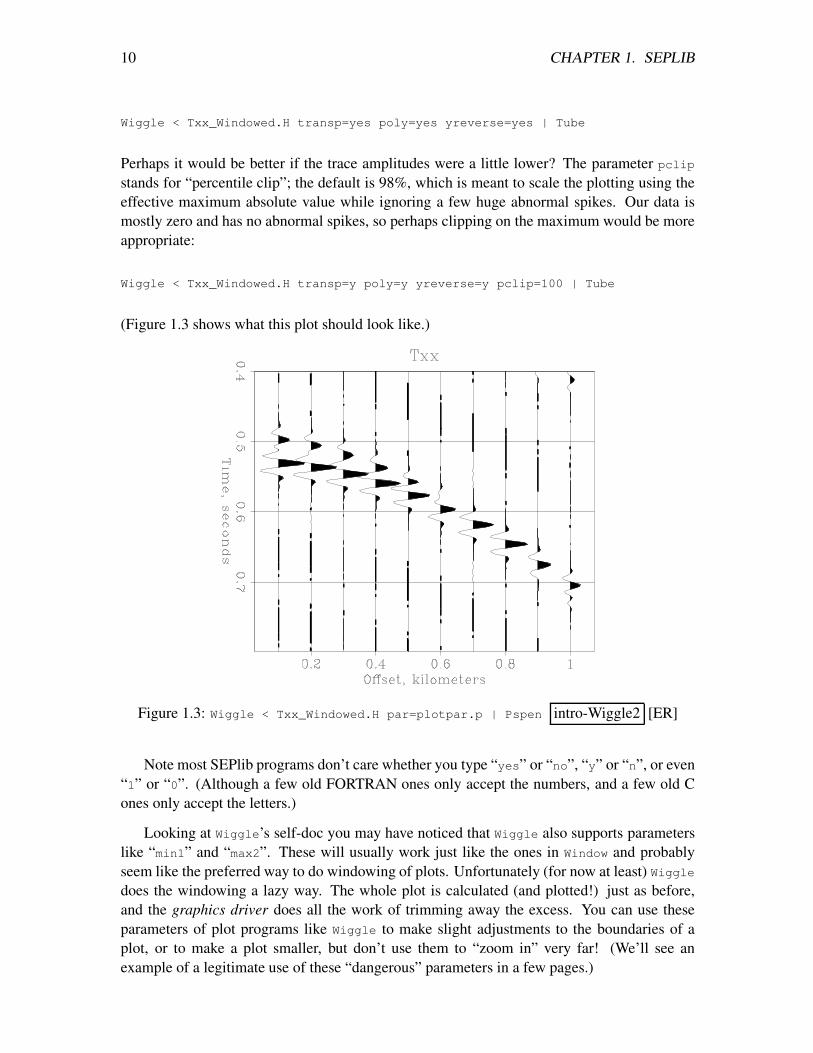
Perhaps it would be better if the trace amplitudes were a little lower? The parameter pclipstands for “percentile clip”; the default is 98%, which is meant to scale the plotting using theeffective maximum absolute value while ignoring a few huge abnormal spikes. Our data ismostly zero and has no abnormal spikes, so perhaps clipping on the maximum would be moreappropriate:
Wiggle < Txx_Windowed.H transp=y poly=y yreverse=y pclip=100 | Tube
(Figure 1.3 shows what this plot should look like.)
Figure 1.3: Wiggle < Txx_Windowed.H par=plotpar.p | Pspen intro-Wiggle2 [ER]
Note most SEPlib programs don’t care whether you type “yes” or “no”, “y” or “n”, or even“1” or “0”. (Although a few old FORTRAN ones only accept the numbers, and a few old Cones only accept the letters.)
Looking at Wiggle’s self-doc you may have noticed that Wiggle also supports parameterslike “min1” and “max2”. These will usually work just like the ones in Window and probablyseem like the preferred way to do windowing of plots. Unfortunately (for now at least) Wiggledoes the windowing a lazy way. The whole plot is calculated (and plotted!) just as before,and the graphics driver does all the work of trimming away the excess. You can use theseparameters of plot programs like Wiggle to make slight adjustments to the boundaries of aplot, or to make a plot smaller, but don’t use them to “zoom in” very far! (We’ll see anexample of a legitimate use of these “dangerous” parameters in a few pages.)
1.3. ILLUSTRATIVE EXAMPLES 11
1.3.2 Parameters, parameter files, and history files
If you find yourself despairing at having to remember and type huge lists of parameters like
transp=y poly=y yreverse=y pclip=100
again and again, you will be happy to know there is a shortcut. Try putting the list of parame-ters above into a text file called “plotpar.p”. Put the windowing parameters
n2=10 n1=200 f1=200
into another file called “windowpar.p”. Then you could do
Window < Txx.HH par=windowpar.p | Wiggle par=plotpar.p | Tube
and it would be just like you had typed the full set of parameters at the “par=plotpar.p” and“par=windowpar.p”. Files like “plotpar.p” and “windowpar.p” are called parameter files,and they can be nested simply by putting par= commands into the parameter files just likeon the command line. An additional advantage of parameter files is that they can be as longas you want, so you don’t have to cram everything onto one single line. (You can also putcomments into a parameter file; anything after a “#” on a line in a parameter file is ignored,just like for csh scripts.)
What happens if the same parameter is set multiple times? The last occurrence is the onlyone that matters. You must pay special attention to how the parameters are written, though: aparameter can be “unset” by leaving the space after the “=” blank. An = with a space before itis ignored completely. In summary:
• n1=1 sets n1 equal to 1;
• n1=1 would unset any previous setting of n1, letting it default.
• n1 = 1 is a comment. It has NO EFFECT AT ALL on n1.
Now reread the previous paragraph again until you are sure you won’t make the mistakeof writing n2 = 10 and wondering why it didn’t work.
You may have already realized that a history file is just a special kind of parameter file.Before checking for parameters on the command line, SEPlib first looks for any relevant pa-rameters in the input history file. That’s how “Wiggle” knew the dimensions of the data inTxx.HH without having to be told. Of course, we can override the information in the inputhistory file by setting another value on the command line. For example, if we do
Wiggle < Txx.HH par=plotpar.p n1=5000 | Tube
12 CHAPTER 1. SEPLIB
Wiggle will happily attempt to read past the end of the floating-point data set, resulting in anerror message
sreed: Illegal seek
Wiggle: xdr error reading from ‘‘in’’
For another example of overriding a parameter set by the history file, how about changingthe title of our plot from the boring “Txx” set in the history file Txx.HH?
Wiggle < Txx.HH par=plotpar.p title="My plot" | Tube
It is also possible to put superscripts, subscripts, etc, into labels and titles; do “man vplot-
text” for examples. Even a single program like Wiggle has more options than we can hopeto enumerate here. To see what other options are possible, look at the self-documentation andtry them out. By all means don’t neglect to check whether the program you are interested inmight happen to have a manual page as well.
Chapter 2
SEP3D Introduction
2.1 SEP3D Overview
The SEPlib software package has proven to be a very productive tool for seismic research andprocessing. However, its usefulness is fundamentally limited to processing regularly sampleddata. This limitation is too restrictive when tackling problems in 3-D seismic and problemsthat involve geophysical data other than seismic. Therefore, we designed and implemented ageneralization of SEPlib to make it capable of handling irregularly sampled data (from nowon we will dub this new version SEP3D, while the old version will be referred to as justSEPlib). In SEPlib, few parameters defined in the history file are sufficient to describe the datageometry, since it is assumed to be regular. In SEP3D, to describe the irregular data geometry,we associate each seismic trace with a trace header, as is done in the SEGY data format, andin its many derivatives. However, to enable users and programmers to deal with irregularlysampled data with the same simplicity and efficiency that is characteristic of SEPlib, SEP3Dintroduces the following two principles:
• Separate the geometry information from the seismic data. This simple but powerful ideais crucial for efficiently processing large amounts of data, such as in 3-D prestack datasets. It allows you to minimize the access to the usually bulky seismic data files, whileperforming many useful operations on the trace headers and on specific subsets of theseismic traces.
• Exploit as much as possible the existing regularity in the data geometry. Regularity isimportant when analyzing and visualizing the data; further, it helps the developmentof simple and efficient code. SEP3D “regularizes” an irregularly sampled data setsby associating the data traces with a uniformly sampled multi-dimensional grid. Thisgridding information is then exploited by SEP3D application and utility programs toefficiently select and access the seismic traces.
Another important characteristic of SEP3D is that it is a generalization of SEPlib and not acompletely new system. There are many good reasons for this choice. From the user point
13
14 CHAPTER 2. SEP3D INTRODUCTION
of view, it enables users familiar with SEPlib to quickly master SEP3D. Further, it enablesSEP3D to leverage the considerable amount of coding and brain power that went into SEPlib.In particular we use the SEPlib routines for accessing files (both ASCII and binary), and buildSEP3D capabilities on the top of these routines.
2.2 Data Format
This section describes the data format of a SEP3D data set. A SEP3D data set is defined asthe collection of all the files (ASCII and binary) that contain the information relevant to theGeophysical data set.
2.2.1 Structure of a SEP3D data set
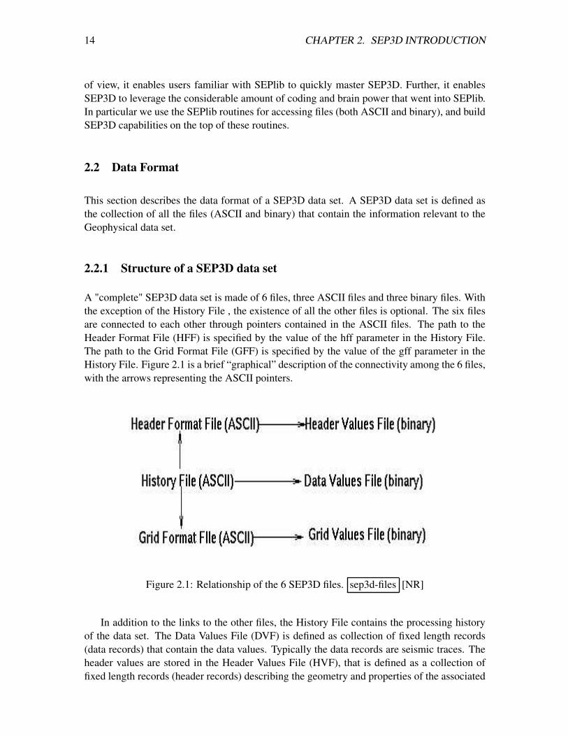
A "complete" SEP3D data set is made of 6 files, three ASCII files and three binary files. Withthe exception of the History File , the existence of all the other files is optional. The six filesare connected to each other through pointers contained in the ASCII files. The path to theHeader Format File (HFF) is specified by the value of the hff parameter in the History File.The path to the Grid Format File (GFF) is specified by the value of the gff parameter in theHistory File. Figure 2.1 is a brief “graphical” description of the connectivity among the 6 files,with the arrows representing the ASCII pointers.
Figure 2.1: Relationship of the 6 SEP3D files. sep3d-files [NR]
In addition to the links to the other files, the History File contains the processing historyof the data set. The Data Values File (DVF) is defined as collection of fixed length records(data records) that contain the data values. Typically the data records are seismic traces. Theheader values are stored in the Header Values File (HVF), that is defined as a collection offixed length records (header records) describing the geometry and properties of the associated
2.2. DATA FORMAT 15
data records. The header parameters are described in the Header Format File by a table ofheader keys. A header keys specifies the name of the header parameter (key name), its datatype (key type), and its position in the header record (key index). The association between theheader records and the data records is described below.
If the data set has been binned on a regularly sampled grid, the Grid Format File containsthe description of the grid. The Grid Value File contains the mapping information betweenthe grid cells and the corresponding header records. The Grid Value File does not exist if thegridding is regular; that is, there is a one-to-one correspondence between grid cells and headerrecords.
2.2.2 Data and Headers Coordinate System
The History File contains the usual SEPlib parameters ni, oi, di, labeli (where i=[1,2,3,...])describing the Data Coordinate System. The length of the axes in the Data Coordinate Systemmust be constant and is given by the values of the respective ni parameter. The number of datavalues in a data record is given by n1 and the the number of data records is equal to the product(n2*...*ni*...). The Header Format File contains also the usual SEP3D parameters ni, oi,
di, labeli (where i=[1,2,3,...]) describing the Header Coordinate System. The number ofheader keys in the header records is given by n1 and the the number of header records is equalto the product (n2*...*ni*...).
2.2.3 Mapping between the header records and the data records
In general, the order and number of the data records stored in the Data Values File may bedifferent than the order and number of the header records stored in the Header Values File. Thishappens, for example, if the Header Values File has been reshuffled (e.g. sorted or transposed)while the Data Values File was left untouched. Whether the data and header records arein the same order is indicated by the value of the integer parameter same_record_number
in the History File. The value of same_record_number is equal to 1 if the records are inthe same order, and equal to 0 if they are not. If same_record_number is missing from theHistory File it is defaulted to 1. When the data and header records are in the same order(same_record_number=1), the association between header records and data records is givenby the positions of the records in the respective binary files, and the Data Coordinate Systemcoincides with the the Header Coordinate System. If data and header records are in differentorder the association between data records and header records is assured by the reserved headerkey data_record_number, that contains the data record number of the associated data record.The value of the data record number is defined as equal to the position of the data record inthe Data Values File.
16 CHAPTER 2. SEP3D INTRODUCTION
2.2.4 Gridding information
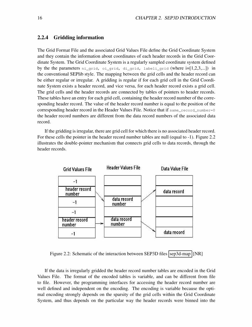
The Grid Format File and the associated Grid Values File define the Grid Coordinate Systemand they contain the information about coordinates of each header records in the Grid Coor-dinate System. The Grid Coordinate System is a regularly sampled coordinate system definedby the the parameters ni_grid, oi_grid, di_grid, labeli_grid (where i=[1,2,3,...]) inthe conventional SEPlib style. The mapping between the grid cells and the header record canbe either regular or irregular. A gridding is regular if for each grid cell in the Grid Coordi-nate System exists a header record, and vice versa, for each header record exists a grid cell.The grid cells and the header records are connected by tables of pointers to header records.These tables have an entry for each grid cell, containing the header record number of the corre-sponding header record. The value of the header record number is equal to the position of thecorresponding header record in the Header Values File. Notice that if same_record_number=0the header record numbers are different from the data record numbers of the associated datarecord.
If the gridding is irregular, there are grid cell for which there is no associated header record.For these cells the pointer in the header record number tables are null (equal to -1). Figure 2.2illustrates the double-pointer mechanism that connects grid cells to data records, through theheader records.
Figure 2.2: Schematic of the interaction between SEP3D files sep3d-map [NR]
If the data is irregularly gridded the header record number tables are encoded in the GridValues File. The format of the encoded tables is variable, and can be different from fileto file. However, the programming interfaces for accessing the header record number arewell defined and independent on the encoding. The encoding is variable because the opti-mal encoding strongly depends on the sparsity of the grid cells within the Grid CoordinateSystem, and thus depends on the particular way the header records were binned into the
2.3. SEP3D STANDARDS 17
Grid Coordinate System. The gridding tables can be stored and retrieved by using the func-tions sep_get_grid_window and sep_put_grid_window described in the SEPlib man and htmlpages.
The Grid Format File and the Grid Values File are optional. When no Grid Format Fileis associated with a data set, the Grid Coordinate System is assumed to be the same as theHeader Coordinate System, and the grid coordinates of the header records are assumed to beregular.
2.3 SEP3D Standards
2.3.1 Standard header names
SEP3D uses many standard header names. These are listed with a short description as follows:
offsetx, offset_x the offset location in x
offsety, offset_y the offset location in y
cmpx, cmp_x the CMP location in x
cmpy, cmp_y the CMP location in y
sx, s_x the source location in x
sy, s_y the source location in y
sz, s_z the source location in z
gx, g_x the receiver location in x
gy, g_y the receiver location in y
gz, g_z the receiver location in z
azimuth the azimuth
aoffset the absolute offset
2.4 Superset
SEP3D is good at dealing with 3-D data, but requires a significant coding overhead. As a resultClapp and Crawley (1996) wrote SEPF90, a Fortran90 library that simplified dealing with 3-Ddata. Unfortunately the design, like all early prototypes, had serious limitations. Among them,
18 CHAPTER 2. SEP3D INTRODUCTION
• it forced referencing through a structure to access the data (something that was incredi-bly slow with early Fortran90 versions)
• it required programs to be written in Fortran90 (even though many programs are moresuited for C)
• it did not easily allow for headers and data to be read separately (a very powerful optionin SEP3D)
The new version of SEPlib comes with a replacement for SEPF90, superset. The purposeof superset is the same, but the implementation is significantly different. The basic ideaof superset is to maintain an invisible sep3d structure copy of each SEP3D dataset. Thestructure contains
• the type of data (float, complex, byte, integer)
• the type of SEP3D file (regular, header, grid)
• the axes of the data (n,o,d,label,unit)
• the header keys associated with the data (key name, key type, key format)
• current section of the grid being processed
• current section of the headers being processed
• mapping from the headers to the traces
This internal structure can be initialized through a SEPlib tag, from another structure, or cre-ated manually by the programmer. Information is passed to and from the structure through asep3dtag.
Reading of any SEPlib data then can be done in two simple steps: First the programmermakes a call to read in the headers (either all or a portion) and is returned the number ofheaders read. The library will automatically read in the grid, find the valid headers, check fora data_record_number and create a list of pointers to the traces. Once the headers have beenread the user can ask for all of the data associated with the header block to read in, or read insections of the data.
Writing is also simple. The programmer first initializes the output format files. He thenmakes a call(s) to write data (data, headers, and/or grid), and finally asks for the number oftraces in the dataset to be updated in the format files if it wasn’t known until the end of theprogram. The library does all the work figuring out what files to write, what trace number it iscurrently writing out, etc.
For added convenience we also have a F90 module which provides wrappers around the Cfunction calls. The module allows the programmer to access a Fortran90 type which containsall properties of the dataset (except the header and grid values). The programmer can thenaccess and modify these values. When done they can synchronize the C and Fortran90 version.This added flexibility further simplifies dealing with SEP3D data.

2.4. SUPERSET 19
REFERENCES
Clapp, R. G., and Crawley, S., 1996, SEPF90: SEP–93, 293–304.

20 CHAPTER 2. SEP3D INTRODUCTION
Chapter 3
Programs
3.1 SEPlib programs
This chapter gives brief descriptions of almost all of the SEPlib programs that come with thestandard SEPlib release for widespread distribution. A few closely related non-SEPlib vplotutilities have been included as well, at the end. To find out more, read the self-documentation.Most programs do not have manual pages (or very current manual pages), so if you needto know more than what you find in the self-doc you’ll probably have to look at the sourcecode. The graphical language used by these programs is called “vplot”. SEPlib’s “vplot” hasabout as much to do with Versatec’s “vplot” as calculus does with roman numerals. See thereferences for some articles describing vplot. While vplot does have several technical manualpages that describe it in great detail, a user’s guide is unfortunately lacking. Note that theNames of these Programs all begin with an Upper-Case Letter.
Add A versatile program for doing element-by-element mathematical manipulations on oneor more data files. It can be used to form linear combinations of two or more files,multiply two or more files, or divide one file by another. It can also be used to scale afile or take the absolute value, square root, logarithm, or exponential.
Again Take the arctangent of a floating-point data file element by element.
Agc Automatic gain control with first-arrival detection.
AMO Azimuth Moveout - Convert from one azimuth and offset to another.
Aniso2d Two-dimensional anisotropic heterogeneous elastic modeling.
Attr Displays the attributes of a dataset.
Balance Perform trace balancing.
Bandpass Butterworth bandpass filtering. See also Lpfilt.
21
22 CHAPTER 3. PROGRAMS
Box Box outputs the vplot commands to draw a balloon-style label. Options let you positionthe box and pointer, control the size of the labeling, etc. (It is even possible to drawboxes with perspective.) The boxes can be overlayed onto vplot graphics files usingthe “erase=once” option of pen filters. The interact option of pen filters can be used todetermine the coordinate of the spot the box’s pointer is to point at. (Alas, not all penfilters support the “interact” capability.) The special pen filter Vppen can be used tocombine vplot files.
Byte Convert floating-point SEPlib data (esize=4) to byte-deep SEPlib raster data (esize=1).Usually used in conjunction with Ta2vplot or X11movie. The clip value is determinedby the option “pclip” for “percentile clip”. pclip=50 gives the median, pclip=100 themaximum, etc. The percentile clip can be calculated based on one particular input panelor all the input panels. (It is also possible to simply specify your own clip, which canspeed the program up tremendously.) The input data is assumed to be about equallysplit between positive and negative values; an option is available for mapping input datathat is all positive to the entire possible range of output values. Several other conversionoptions are available that are useful for bringing out hidden features in data, such as asign-preserving gain parameter “gpow”.
CAM Common Azimith Migration.
Cabs Complex (esize=8) to real (esize=4) conversion; take the absolute value of complex-valued data. (Alternatively, if you consider the input data to be (X,Y) coordinate pairs,output the Euclidean norm.)
Cat Combine two or more SEPlib header files into one by concatenation. They can be mergedalong either the fast (1), intermediate (2), or slow (3) axes.
Cfft Complex fast-Fourier transform. Requires complex-valued input data (esize=8).
Clip Find a “clip” value for the input data, and put it into the header. With appropriate optionsperforms several sorts of clipping on the data as well, such as changing all clipped orunclipped values to some given value, etc. The clip value is determined by the option“pclip” for “percentile clip”. pclip=50 gives the median, pclip=100 the maximum, etc.
Cmplx Combine two real (esize=4) data files into one complex data file (esize=8). Notethat some programs such as Graph treat esize=8 data files as (X,Y) coordinate pairs, sothis program can also be thought of as a way to combine an “X” and a “Y” file into an“(X,Y)” file. See also Real and Imag.
Combine Combine two sets of elastic layer coefficients to give the effective combined layer.
Conj Take the complex conjugate for each element of a complex-valued dataset. (I.E., changethe sign on the second real number in each element of an esize=8 dataset.)
Contour Input a real-valued (esize=4) dataset and output vplot commands for a two-dimensionalcontour plot of the data. (The vplot output can be viewed on a screen using the programTube, or plotted on a postscript printer using Pspen.) Contour has many, many options
3.1. SEPLIB PROGRAMS 23
to specify at what values to draw contours, where to position the plot on the page, howbig to make the plot, which way to draw the axes, where to place tick marks and labels,etc, etc, etc. All of these parameters attempt to default reasonably. Contour also al-lows auxiliary input files which can be used to annotate the contour plot with symbols,curves, or arrows. You may find the utility programs Window and Reverse useful forpre-processing data to be plotted with Contour. See also Vppen and Box for a crudeway of adding annotation, and plas and pldb for a crude way of editing.
Cp Copy a SEPlib dataset.
Create Create a stiffness tensor given lambda and mu, or p-wave velocity and s-wave velocity,or all of the elastic coefficients.
Cubeplot Create a 3D raster plot of a seismic data cube.
Dd Convert data from one esize to another. Possibilities for esize are 0 (ASCII), 1 (byte-deepraster), 2 (short integer), 3 (real with least-significant byte truncated), 4 (real), and 8(complex). Dd currently attempts to perform all conversions in core, so it is only usefulfor converting relatively small datasets.
Decon Perform deconvolution. Choices of predictive, Lomoplan, steep dip. Uses the helixand patching.
Disfil Formatted display of a binary data file. Allowable input types are real (both IEEE andnative), integer, complex, and byte. The default depends on the input esize but can beoverridden from the command line. There are several options that can be used to controlthe format of the output ASCII data if you don’t like the default. There are also optionsfor changing the reading frame or only showing some subset of the input data. Thedefault is to start at the beginning and show everything.
Display Take a layer parameters dataset and display the parameters.
Dots A program somewhat like Wiggle, but better in some ways because it tries to be smarter.The output style depends on the input n1 and n2. For loosely packed traces with onlya few data points Dots plots the data as lollipops on strings, showing each data pointclearly. There are also options for separately labeling each trace, omitting dead traces,making bar graphs, etc. As n1 and n2 increase Dots by default simplifies the output andeventually behaves almost the same as Wiggle. Unfortunately Dots does not use theaxis drawing and plotting routines shared by Wiggle, Contour, Graph, and Ta2vplot,and so Dots’ options and output plot size, position, and axes are currently incompatiblewith those for other plot programs.
Energy Calculate energy in running windows along fast axis of data.
Envelope Calculate signal amplitude.
FMeikonal Fast marching eikonal solver.
24 CHAPTER 3. PROGRAMS
Filter Filtering along the fast axis performed in the frequency domain. The filter is read froman auxiliary input file. (This old FORTRAN program does not do dynamic allocation;the input trace length is hardcoded to a limit of 4096 samples.)
Ft3d One, two, or three-dimensional Fast Fourier transform. The input and output are complex-valued (esize=8). The sign of the Fourier transform on each axis can be set from thecommand line or history file. Ft3d writes the opposite sign onto the output history fileso a second application will automatically perform the inverse of the first. A sign of0 skips transforming on that axis entirely. There are options to allow centering of theorigin in the output domain, to make a graph of the output easier to understand.
Ftplot Output vplot commands to plot an input real time series and its Fourier amplitude orphase spectrum.
Fx2d 2D Fx deconvolution.
Gauss Create Gaussian anomalies for a velocity model.
Get Perform simple operations on parameters.
Gfgradz Calculate Green’s functions for a v(z) medium.
Gpow Raise each element of an input data file to a power, preserving sign. The power to usedefaults to unity, so you probably want to specify it.
Graph The standard SEPlib program for making graphs of all sorts. The input data canbe real numbers (esize=4) or coordinate pairs (esize=8). (See Cmplx for convertingseparate X and Y files into one (X,Y) file.) The output will consist of n3 graphs, eachplotted with their own axes set according to the data in that graph. Each graph willhave n2 traces with n1 points in each trace. (Although if the option is set then n3
will effectively become n1*n2 and n2 will become one.) If esize=8 the (X,Y) pairsdetermine the coordinates to draw. If esize=4 the input value is taken as the Y of thepair, as you would expect, while the input d1, o1, and element number are used tocalculate the associated X. Graph supports a bewildering variety of plotting options;almost every part of the plot can be moved about or turned on and off. The colors,symbols, line styles, line fatnesses, etc, for each trace can be specified. There are optionsto set the background screen color and the background graph color. Notably lacking isa mechanism for overlaying labels on the graph. (This is possible to do in a somewhatcrude way by simply creating a vplot file with labels in the appropriate position usingBox, and appending the plot containing the annotations onto the vplot file containingthe graph using Vppen.) Graph sets the output clipping window hard against the limitof its graphing area, so the slightest bug in the positioning of the clipping window by theoutput “pen” filter may clip away extreme parts of the plot. (Single-pixel-off clippingwindows is a bug that is unfortunately all too common among “pen” filters, so you willprobably see this bug sooner or later.)
Grey Create a raster vplot. This is used alot. Has many optional color tables.
3.1. SEPLIB PROGRAMS 25
Halfint Half-order integration along the fast axis. (Also conjugate and inverse of this opera-tion. The inverse is half differentiation.)
Headermath Perform mathematical operations on header keys.
Helderiv Factor the laplacian operator. Apply helix derivative. Loops over n3.
Helicon Apply helix convolution (polynomial multiplication) or deconvolution (polynomialdivision). One is the exact inverse of the other. Beware of helical boundary conditions.
Histogram Create a histogram of the dataset’s frequency distribution.
Hwt2d Create a 2-D ray database via Huygens wavefront tracing.
Hwt3d Create a 3-D ray database via Huygens wavefront tracing.
Hypint Velocity-space transformation via integration (along hyperbolas). (Also does conju-gate transpose and pseudo-inverse; the conjugate transpose is hyperbola superposition.)
Hypmovie Create a movie going in and out of velocity space.
Hypsum Velocity-space transformation via superposition (along hyperbolas).
Imag Convert from complex (esize=8) to real (esize=4) by keeping only the imaginary com-ponent. Alternatively, pull the Y component out of (X,Y) coordinate pairs.
In Give useful information about a SEPlib header/data file pair. Tells you which of the canon-ical parameters are set in the header file and which are defaulted, and what values theyhave. Tells you the expected size of the data given the header and whether the datais actually that size. (Very useful if you want to check on the progress of a runningprogram.) Warns if the data is all zeroes. Etcetera. Unlike most SEPlib programs, Inunderstands four-dimensional datasets.
Interleave Merge two files on the 2-axis (1 axis is fast, 3 is slow) by interleaving them.
Interp Linear interpolation on the 2-axis. (Also can do the conjugate, transpose, and pseu-doinverse of this operation.)
Iso2d 2-d isotropic modeling.
LMO Perform linear moveout.
Laymod Create elastic parameter model of a layer with interbedding layers.
Laymod21 Create elastic parameter model of a layer with interbedding layers, output is 21panels, one for each of the independent elastic constants divided by the density.
LoLPef Find PEF on aliased traces (with patching).
Log Take the log of data.
26 CHAPTER 3. PROGRAMS
Lomiss Fill in missing data by mimimizing the data power after convolution. Works in anynumber of dimensions!
Lopef Estimate local prediction-error filters with the helix and patching.
Lpfilt Butterworth lowpass filtering. See also Bandpass.
Ls List the data files associated with the given header files. (Also useful for directly referringto the data file associated with a SEPlib header file, so you can use SEPlib data files asinput to non-SEPlib programs. For example instead of you could do .)
MCvfit Monte Carlo automatic velocity picks (fit).
MTTmaps Band-limited maximum-energey Green’s function maps.
Math Perform mathematical operations on data.
Median Apply a median smoother.
Miss Perform missing data interpolation with a prescribed helix filter.
Mute Mute a SEPlib dataset.
Mv Copy (not move, despite the name) a SEPlib header and data file to another name. Theoutput history file name is set on the command line; the associated data file name isdetermined by the usual rules (involving environment variable, the name of the historyfile, etc.).
NMO Standard Normal MoveOut correction via linear interpolation; also can do the conju-gate and pseudoinverse of this operation. Make sure to specify a reasonable velocity(or velocity function) for it to use. It wants NMO velocity, not interval velocity; by allmeans make sure to get the units right!
Noise Add random noise to data, either Gaussian or uniform.
OFF2ANG Convert from offset to angle domain or back for wave equation migration.
Operplot Plot a one-, two- or, three-dimensional set of samples.
Overlay Draw a simple overlay (polylines, text, boxes, and ovals).
Pad Append zeroes onto any of the fast (1), intermediate (2), or slow (3) axes to make aSEPlib file bigger. Defaults to bump up to the next power of two. Also can appendzeroes onto the “0” axis, for example it pads esize=4 to esize=12 by appending twofloating-point zeroes onto each element.
Pef Estimate a PEF in N dimensions.
Phase Phase-shift migration and diffraction.
Pow Raise data to a power, preserving sign.
3.1. SEPLIB PROGRAMS 27
Pspen The vplot “pen” filter for postscript devices.
Radial Transform to radial traces. Also can do the conjugate and pseudoinverse of this oper-ation.
Radnmo Transform to radial traces and do NMO at the same time. Also can do the conjugateand pseudoinverse (for constant velocity) of this operation.
Real Convert from complex (esize=8) to real (esize=4) by keeping only the real component.Alternatively, pull the X component out of (X,Y) coordinate pairs.
Reshape Reshape a SEPlib dataset. Usually this will involve shifting axes for use with otherSEPlib programs. The user must ensure that the amount of data in equals the amount ofdata out. For example, if we have a datset of dimensions n1=10 n2=10 n3=10 and runthis command: Reshape < in.H >out.H axis3=axis2 axis4=axis3 n2=1, we result-ing dimensions will be n1=10 n2=1 n3=10 n4=10.
Reverse Flip one or more axes of the dataset.
Ricksep The ultimate movie program. Displays seismic data sets with 3 or more dimensions.
Rickvel Ricksep modified to do picking for velocity analysis.
Rm Remove a SEPlib header file and its associated data file. Not to be confused with lower-case .
Rotate Rotate the coordinate frame of the elastic coefficients for a layer to give a new layer.
Rtoc Real (esize=4) to complex (esize=8) conversion; the imaginary part is set to zero. Thisfunction can also be done as a special case of Pad.
Scale Trivial data scaling program; multiply a dataset by the parameter “dscale”. (Bewarethe special-case behavior of “dscale=1”!) Add can also be used to scale a dataset, butAdd cannot use pipes which makes it somewhat less convenient. Unlike Add, Scale canbe used to automatically normalize a dataset so the maximum is (plus or minus) unity.(There are several options governing how much of the dataset is to be normalized at atime.)
Smooth Perform smoothing.
Spectra/Spectrum Calculate average Fourier-domain amplitude spectra. Accepts real orcomplex input.
Spike Everyone’s favorite program for creating a SEPlib dataset out of thin air. Can be usedto create a dataset that is all zeroes, all ones, or all some specified constant value. It ismost often used to create a dataset that is mostly zeroes except for one or more “spikes”of unit magnitude. Beware the FORTRAN-style notation: the first element is numbered1, not 0, as it would be for most other SEPlib programs.
Stack Sum a dataset over the intermediate (2) axis.
28 CHAPTER 3. PROGRAMS
SRM Stolt Residual Migraion
Stretch A general t-squared x-squared stretching and conversion program that is usuallycalled under one of the aliases NMO, Unmo, Radnmo, Radial, or Stolt.
Surface Creates surfaces described by parametric curves. Makes fun velocity models.
Ta2vplot Input a SEPlib raster (esize=1) dataset and output vplot commands for a two-dimensional raster plot of the data. (The vplot output can be viewed on a screen usingthe program Tube, or plotted on a postscript printer using Pspen.) Ta2vplot has many,many options to specify generic plotting things such as where to position the plot on thepage, how big to make the plot, which way to draw the axes, where to place tick marksand labels, etc, etc, etc. All of these parameters attempt to default reasonably. There arealso several options unique to Ta2vplot to control things such as orientation of the rasterand what color table to use (user-specified color tables are allowed). Ta2vplot also ac-cepts esize=3 input which it interprets as (R,G,B) byte-deep triples. This option is mostuseful for plotting raster that is meant to have a “multidimensional” color table. (Warn-ing: the esize=3 option is very slow if used with the standard linear Movie-style colortables, although it does work. esize=3 input is really meant to be used with “RGB”color tables.) You may find the utility programs Window and Reverse useful for pre-processing data to be plotted with Ta2vplot. See also Vppen and Box for a crude wayof adding annotation.
Taplot A synonym for Byte.
Thplot Pseudo three-dimensional hidden-line plotting program.
Tpow Multiply each element of a seismogram by time raised to a given power. (The dimen-sion associated with the fast (1) axis is assumed to be time.) A power of 2 often seemsto be a good one for balancing the early and late time of a seismogram without the lossof amplitude information and other annoying problems associated with automatic AGC.(By default Tpow attempts to find a good default value for the time-power parameterautomatically. Unfortunately the routine that does this has been broken by a carelessprogrammer and currently always core dumps; for now (mid 1992) you must specifythe tpow yourself.)
Transf Transpose and FFT a dataset.
Trcamp Calculate total energy in a tapered time window.
Transp Transpose two of the three dimensions of a SEPlib data cube. (An option lets youselect which two.)
Tube The generic vplot “pen” filter for screen devices. (In reality it’s just a script that callsthe appropriate pen filter for your device by searching case-by-case for the value ofyour environment variable in a switch.) The “pen” manual page gives a canonical list ofdevice-independent Tube (and tube) options. Additional options may apply, dependingon which pen filter Tube calls.
3.1. SEPLIB PROGRAMS 29
Txdec TX domain noise removal, 2- or 3-D.
Uncombine Subtract the second set of layer coefficients from the first to give a new set.
Uncrack Compare a fractured layer with an unfractured sample of the same rock and printout the excess compliance.
Unmo The pseudoinverse of the program NMO (standard Normal MoveOut correction vialinear interpolation). Make sure to specify a reasonable velocity for it to use!
Vconvert Convert one type of velocity function to another (interval/rms and depth/time con-versions).
Vel Make a velocity model.
Velan Velocity analysis of common-midpoint gathers.
Vppen The vplot “pen” filter for the virtual vplot device. This program is widely used to dovarious utility sorts of transformations on vplot files. It can be used to automaticallycenter and size vplot files, to report statistics, rotate, scale, shift, fatten, thin, scale text,scale dash patterns, etc, etc, etc. It can also be used to combine multiple vplot files invarious ways. For example it can overlay one vplot file on top of another, combine themas successive frames in a single file, or most usefully combine multiple plot frames intoone superplot by arranging the individual subplots in a grid. As you can guess, Vp-pen has a frightening number of options; they are enumerated with some explanationin both the vppen and pen man pages. (These man pages are at least current and com-plete, though some people have claimed that they are just too dense and wordy to beusable.) See also vppen (lower case), plas, pldb, and the vplot manual pages (vplot,pen, vplottext, vplotraster, libvplot).
Wavelet Wavelet generation program; used by modeling programs as input to provide asource time function. Beware the dreaded “echo” bug that can occur if the output timeduration is too much longer than the duration of the wavelet. (After the wavelet is zeroand should remain forevermore zero, a new scaled-down copy of the wavelet fires offagain.)
Wiggle Inputs a real-valued (esize=4) dataset and outputs vplot commands for a geophysical-style wiggle plot of the data. (The vplot output can be viewed on a screen using theprogram Tube, or plotted on a postscript printer using Pspen.) Wiggle has many, manyoptions to specify how closely to pack the plot traces, how much to overlap the wiggles,whether to fill under the positive excursions, where to position the plot on the page, howbig to make the plot, which way to draw the axes, where to place tick marks and labels,etc, etc, etc. All of these parameters attempt to default reasonably, although Wiggle canbehave stupidly if the input data is constant or consists mostly of zeroes. In such casesyou may have to set the clip value yourself. You may find the utility programs Windowand Reverse useful for pre-processing data to be plotted with Wiggle. See also Vppenand Box for a crude way of adding annotation. Also see the related program Dots,which is superior to Wiggle for some applications.
30 CHAPTER 3. PROGRAMS
Window Window out a portion of a dataset. This includes dropping elements from the begin-ning or end of an axis (or both); it also includes decimation. The beginning and endingelements can be specified in terms of physical units (dependent on the “o” and “d” pa-rameters of the axis) or in terms of element number. Note Window, like most SEPlibprograms, uses “C” style numbering: the first element is numbered 0, not 1 as may seemnatural to you if you grew up on FORTRAN. Beware the special-case behavior of Win-dow if one of the axes is reduced to length 1: it automatically does a transpose to shiftunit-length axes to the end. This behavior is usually desirable, but can be an unpleasantsurprise if unexpected. (If not desired there is an option to turn it off.) Unlike mostSEPlib programs, Window understands four-dimensional datasets.
Xtpen The X11 “pen” device. One of the snazziest vplot filters around.
Zero Create file(s) of zero length.
3.1.1 Useful non-SEPlib programs
Note that the names of these programs all begin with a lower-case letter.
plas plas reads in a human-readable ASCII version of the vplot graphics language and writesout standard binary vplot (the same stuff written into the output SEPlib data file bySEPlib graphics programs like Graph, Wiggle, Contour, Ta2vplot, Dots, etc...). plasis the inverse of pldb. plas is primarily used to convert the output of pldb back intoregular vplot, but it can also be used to generate trivial vplot files from scratch. To dothis, use your favorite editor to create an ASCII human-readable version of a vplot file,then use plas to turn it into a genuine (binary) vplot file. You can find the documentationfor both the ASCII and binary vplot file formats in the vplot man page, although it isprobably easier to learn by using pldb to generate a few examples from known files.(Note plas is not a SEPlib program: it does not begin with a capital letter. It does notread in or write out SEPlib history files!)
pldb pldb reads a vplot file from standard input (not a SEPlib header file pointing to a vplotdata file, but a raw vplot data file) and writes out a human-readable and editable ASCIIversion. By default the units are in integer “vplot units”, 600 to the inch. You mayfind the options of pldb to express everything in units of inches or centimeters make theoutput ASCII vplot file easier to work with. pldb is often used to perform trivial editingoperations on a vplot graphics file. For example, if you want to change the color of someobject and can’t easily regenerate the plot from scratch, you can convert the binary vplotto ASCII using pldb, edit one or two lines so the color changes and changes back againat the right times, and then use plas to turn the file back into standard binary vplot.(Note pldb is not a SEPlib program: it does not begin with a capital letter. It does notread in or write out SEPlib history files.) See also plas (the inverse of pldb).
pspen The non-SEPlib version of Pspen; takes straight vplot files as input instead of SEPlibhistory files that point to vplot files.
3.2. SEP3D PROGRAMS 31
tube The non-SEPlib version of Tube; takes straight vplot files as input instead of SEPlibhistory files that point to vplot files.
vp_Movie Create a movie of vplot files.
vp_Overlay Overlay many vplot files one over another.
vp_OverUnderAniso Stack two or more vplot plots one over the other, with the first onbottom and the last on top. Stretch the files anisotropically to “fill the screen”. Themultiple plots to be stacked can be spread through multiple input files, or can be multipleframes of plots (separated by erases) within a single vplot file.
vp_OverUnderIso Stack two or more vplot plots one over the other, with the first on bottomand the last on top. Do not stretch the files to “fill the screen”; preserve aspect ratios.The multiple plots to be stacked can be spread through multiple input files, or can bemultiple frames of plots (separated by erases) within a single vplot file.
vp_SideBySideAniso Like vp_OverUnderAniso, but stacks plots side by side from left toright.
vp_SideBySideIso Like vp_OverUnderIso, but stacks plots side by side from left to right.
vp_Unrotate Unrotate old-style plots. (In former days SEPlib programs put the plot originat the upper-left corner of the screen, with the X axis going down and the Y axis goingleft to right across the page.) Hopefully you will never have a need for this utility, butthe past never completely dies.
vppen The non-SEPlib version of Vppen; takes straight vplot files as input instead of SEPlibhistory files that point to vplot files. The user interface to vppen can be intimidat-ing to the new user. Those intimidated may find the shells vp_OverUnderAniso,vp_OverUnderIso, vp_SideBySideAniso,vp_SideBySideIso, and vp_Unrotate useful. These shells use vppen to do their workbut have a much simpler user interface (since they aren’t trying do to everything underthe sun in one program). See also plas, pldb, tube, and the vplot manual pages.
3.2 SEP3D programs
Many of the programs described in the previous section can be used on SEP3D datasets aswell, but there are some programs that have been modified for SEP3D or are only compatiblewith SEP3D datasets. These are listed here. Note that they all begin with Capital Letters andmost end in 3d.
Attr3dhead Calculates statistics for header values of SEP3d dataset.
Cat3d Concatenate SEP3D datasets. It also has a “virtual” option if you don’t really want toconcatenate the files but do want a multi-file SEP3D file.
32 CHAPTER 3. PROGRAMS
Cp3d Copy SEP3D datasets.
Create3d Create a SEP3D file from either two SEPlib files or a single SEPlib file.
Dis3dhead Display header values for a SEP3D dataset.
Fold3d Calculate the fold of SEP3D dataset.
In3d Provide useful information about SEP3D datasets.
Infill3d Stack a SEP3D dataset producing a normalized SEPlib cube.
Kirmod3d Perform Born/Kirchhoff modeling.
Marine_geom3d Make TRACE HEADERS for simple Marine Geometries both in CMP andshot gather sorts.
Mv3d Move a SEP3D dataset.
Nmo3d Perform NMO, adjoint NMO, pseudoinverse NMO on a SEP3D dataset.
Rm3d Remove all files of a SEP3D dataset.
Scat3d Create a 3-D scatter model for Kirmod3d.
Sort3d Sort, transpose, or test gridding parameters.
Stack3d Stack a SEP3D dataset.
Synch3d Synchronize headers and data of a SEP3D dataset.
Velan3d Perform Velocity Analysis on sep3d datasets.
Window3d Window SEP3D datasets.
Window_key Window SEP3D headers dataset according to key values.
3.3 Graphics programs
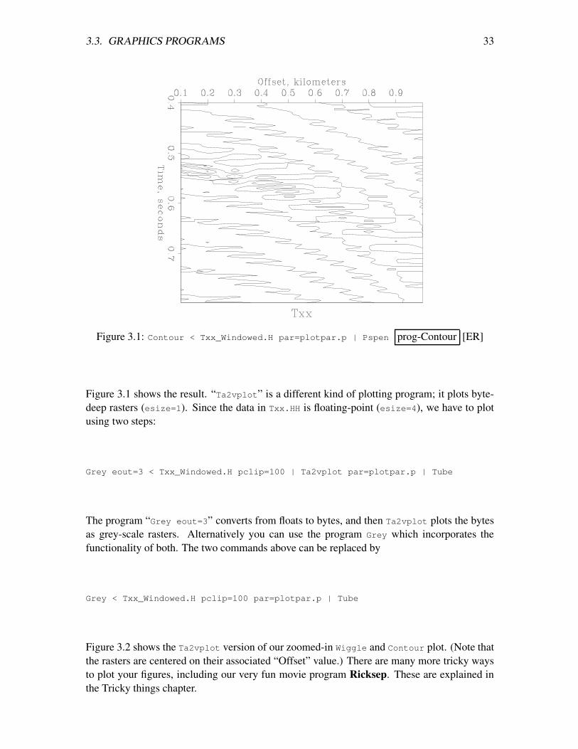
You must be getting bored of wiggle plots by now, and we also want to show how once youget a feeling for SEPlib it is really easy to get around with new programs too. So, how aboutchoosing another form of display? How about a contour plot instead? We know that it mightsound strange to contour seismic traces, but let’s try it! All we want to do is to demonstratethat since the plotting programs have a consistent interface, it is as simple as:
Contour < Txx_Windowed.H par=plotpar.p | Tube
3.3. GRAPHICS PROGRAMS 33
Figure 3.1: Contour < Txx_Windowed.H par=plotpar.p | Pspen prog-Contour [ER]
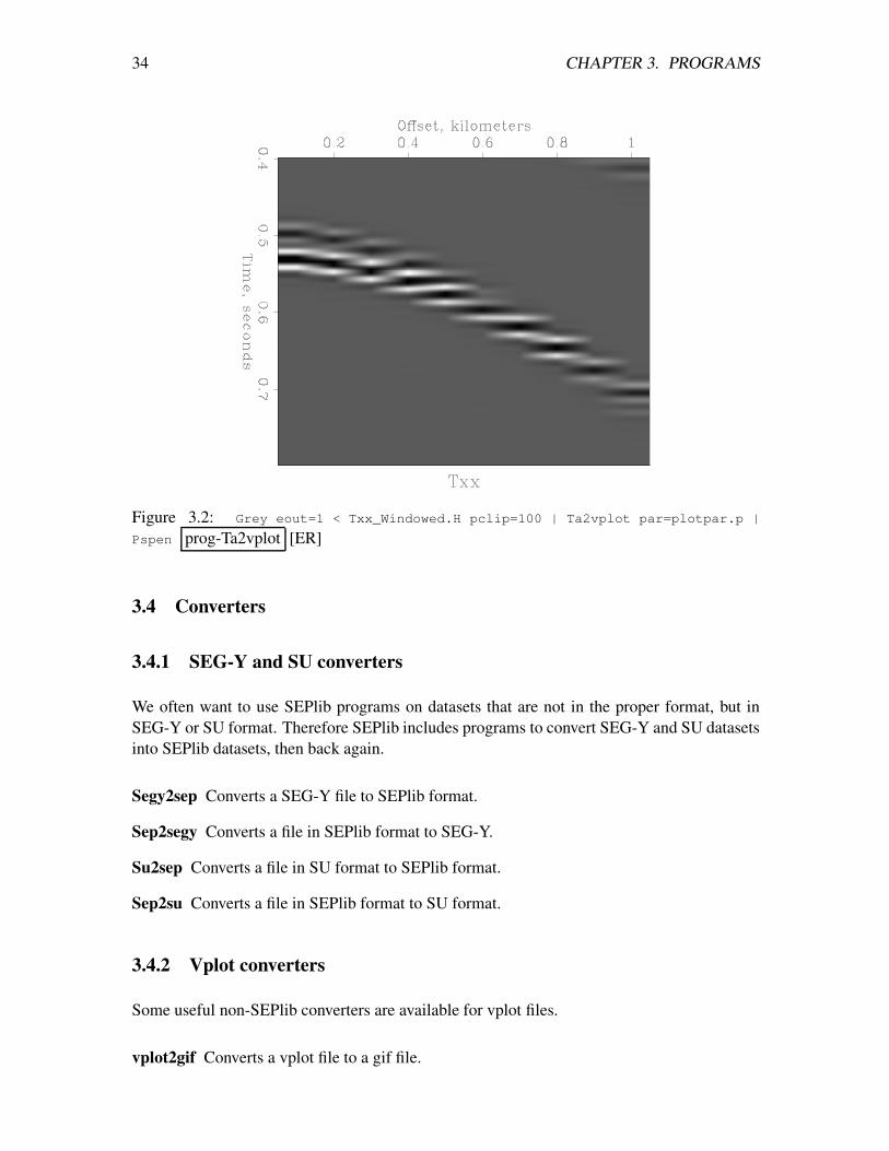
Figure 3.1 shows the result. “Ta2vplot” is a different kind of plotting program; it plots byte-deep rasters (esize=1). Since the data in Txx.HH is floating-point (esize=4), we have to plotusing two steps:
Grey eout=3 < Txx_Windowed.H pclip=100 | Ta2vplot par=plotpar.p | Tube
The program “Grey eout=3” converts from floats to bytes, and then Ta2vplot plots the bytesas grey-scale rasters. Alternatively you can use the program Grey which incorporates thefunctionality of both. The two commands above can be replaced by
Grey < Txx_Windowed.H pclip=100 par=plotpar.p | Tube
Figure 3.2 shows the Ta2vplot version of our zoomed-in Wiggle and Contour plot. (Note thatthe rasters are centered on their associated “Offset” value.) There are many more tricky waysto plot your figures, including our very fun movie program Ricksep. These are explained inthe Tricky things chapter.
34 CHAPTER 3. PROGRAMS
Figure 3.2: Grey eout=1 < Txx_Windowed.H pclip=100 | Ta2vplot par=plotpar.p |
Pspen prog-Ta2vplot [ER]
3.4 Converters
3.4.1 SEG-Y and SU converters
We often want to use SEPlib programs on datasets that are not in the proper format, but inSEG-Y or SU format. Therefore SEPlib includes programs to convert SEG-Y and SU datasetsinto SEPlib datasets, then back again.
Segy2sep Converts a SEG-Y file to SEPlib format.
Sep2segy Converts a file in SEPlib format to SEG-Y.
Su2sep Converts a file in SU format to SEPlib format.
Sep2su Converts a file in SEPlib format to SU format.
3.4.2 Vplot converters
Some useful non-SEPlib converters are available for vplot files.
vplot2gif Converts a vplot file to a gif file.

3.4. CONVERTERS 35
vplot2mpeg Converts a vplot file to a mpeg file.
vplot2ras Converts a vplot file to a raster file.

36 CHAPTER 3. PROGRAMS
Chapter 4
Ricksep
Ricksep is the next generation of Rickmovie. This chapter includes the full documentationfor Ricksep, but we will first summarize the new features. Ricksep has the ability to showseveral datasets at the same time, linked in such a way as to display the same slices of all ofthe datasets if you select a slice in one dataset. This is particularly useful when comparingdifferent processing flows on the same dataset. There are many parameters available to cus-tomize the display of multiple datasets, but for general use Rickmulti is a script that shows areasonable default multi-dataset display. Note that Rickmulti requires the data cubes to havethe same size dimensions (cube 1 n1=cube 2 n1, cube 1 n2=cube 2 n2, etc.). Ricksep hasan expanded picking function. It allows you to pick several different groups of points usingdifferent symbols for each and write them to the same file. This is useful for picking severaldifferent events in a dataset. Ricksep has an improved annotation option. It allows you todraw ovals and rectangles on the displayed dataset. The coordinates of these shapes can thenbe written out to a file for use with vplot programs. Ricksep has an interactive velocity analysisfunction. It can display the original dataset, a velocity scan, and an NMO-corrected dataset.Different velocity functions can be picked on the velocity scan and the new NMO correctionwill be displayed. Rickvelan is a script that displays these panels correctly.
4.1 Ricksep documentation
Ricksep - display cubic array of data in XWindows-Motif
USAGE: Ricksep in=datafile [ data pars ] [ display pars ]
DATA ARGUMENTS:
in=datafile n1= n2= n3= bytes format (SEPlib)
byte array without header
in=datafile n1= n2= n3= esize=4 float format
float array without header
DATA PARAMETERS:
For all parameters:
First check command line with dataset number (e.g) for the
37
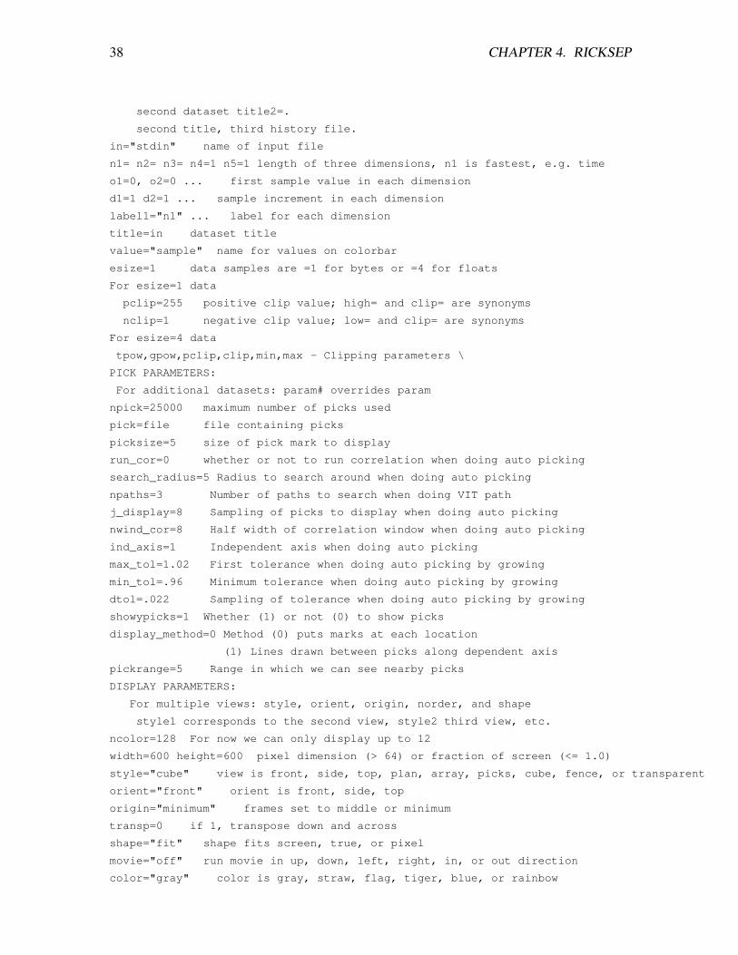
38 CHAPTER 4. RICKSEP
second dataset title2=.
second title, third history file.
in="stdin" name of input file
n1= n2= n3= n4=1 n5=1 length of three dimensions, n1 is fastest, e.g. time
o1=0, o2=0 ... first sample value in each dimension
d1=1 d2=1 ... sample increment in each dimension
label1="n1" ... label for each dimension
title=in dataset title
value="sample" name for values on colorbar
esize=1 data samples are =1 for bytes or =4 for floats
For esize=1 data
pclip=255 positive clip value; high= and clip= are synonyms
nclip=1 negative clip value; low= and clip= are synonyms
For esize=4 data
tpow,gpow,pclip,clip,min,max - Clipping parameters \
PICK PARAMETERS:
For additional datasets: param# overrides param
npick=25000 maximum number of picks used
pick=file file containing picks
picksize=5 size of pick mark to display
run_cor=0 whether or not to run correlation when doing auto picking
search_radius=5 Radius to search around when doing auto picking
npaths=3 Number of paths to search when doing VIT path
j_display=8 Sampling of picks to display when doing auto picking
nwind_cor=8 Half width of correlation window when doing auto picking
ind_axis=1 Independent axis when doing auto picking
max_tol=1.02 First tolerance when doing auto picking by growing
min_tol=.96 Minimum tolerance when doing auto picking by growing
dtol=.022 Sampling of tolerance when doing auto picking by growing
showypicks=1 Whether (1) or not (0) to show picks
display_method=0 Method (0) puts marks at each location
(1) Lines drawn between picks along dependent axis
pickrange=5 Range in which we can see nearby picks
DISPLAY PARAMETERS:
For multiple views: style, orient, origin, norder, and shape
style1 corresponds to the second view, style2 third view, etc.
ncolor=128 For now we can only display up to 12
width=600 height=600 pixel dimension (> 64) or fraction of screen (<= 1.0)
style="cube" view is front, side, top, plan, array, picks, cube, fence, or transparent
orient="front" orient is front, side, top
origin="minimum" frames set to middle or minimum
transp=0 if 1, transpose down and across
shape="fit" shape fits screen, true, or pixel
movie="off" run movie in up, down, left, right, in, or out direction
color="gray" color is gray, straw, flag, tiger, blue, or rainbow
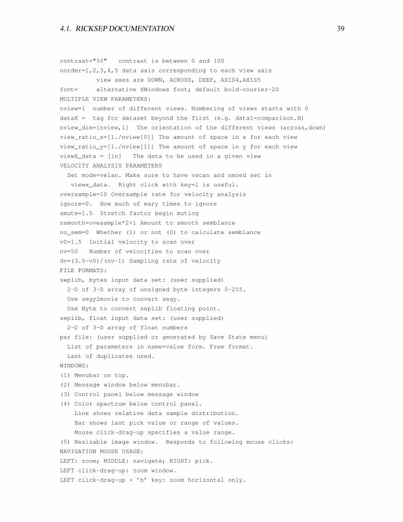
4.1. RICKSEP DOCUMENTATION 39
contrast="50" contrast is between 0 and 100
norder=1,2,3,4,5 data axis corresponding to each view axis
view axes are DOWN, ACROSS, DEEP, AXIS4,AXIS5
font= alternative XWindows font; default bold-courier-20
MULTIPLE VIEW PARAMETERS:
nview=1 number of different views. Numbering of views starts with 0
dataX = tag for dataset beyond the first (e.g. data1=comparison.H)
nview_dim=[nview,1] The orientation of the different views (across,down)
view_ratio_x=[1./nview[0]] The amount of space in x for each view
view_ratio_y=[1./nview[1]] The amount of space in y for each view
viewX_data = [in] The data to be used in a given view
VELOCITY ANALYSIS PARAMETERS
Set mode=velan. Make sure to have vscan and nmoed set in
viewx_data. Right click with key=l is useful.
oversample=10 Oversample rate for velocity analysis
ignore=0. How much of eary times to ignore
smute=1.5 Stretch factor begin muting
nsmooth=ovesample*2+1 Amount to smooth semblance
no_sem=0 Whether (1) or not (0) to calculate semblance
v0=1.5 Initial velocity to scan over
nv=50 Number of velocities to scan over
dv=(3.5-v0)/(nv-1) Sampling rate of velocity
FILE FORMATS:
seplib, bytes input data set: (user supplied)
2-D of 3-D array of unsigned byte integers 0-255.
Use segy2movie to convert segy.
Use Byte to convert seplib floating point.
seplib, float input data set: (user supplied)
2-D of 3-D array of float numbers
par file: (user supplied or generated by Save State menu)
List of parameters in name=value form. Free format.
Last of duplicates used.
WINDOWS:
(1) Menubar on top.
(2) Message window below menubar.
(3) Control panel below message window
(4) Color spectrum below control panel.
Line shows relative data sample distribution.
Bar shows last pick value or range of values.
Mouse click-drag-up specifies a value range.
(5) Resizable image window. Responds to following mouse clicks:
NAVIGATION MOUSE USAGE:
LEFT: zoom; MIDDLE: navigate; RIGHT: pick.
LEFT click-drag-up: zoom window.
LEFT click-drag-up + ’h’ key: zoom horizontal only.
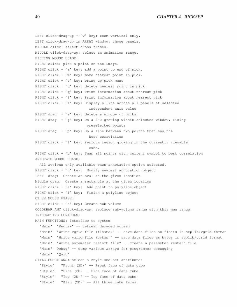
40 CHAPTER 4. RICKSEP
LEFT click-drag-up + ’v’ key: zoom vertical only.
LEFT click-drag-up in ARRAY window: those panels.
MIDDLE click: select cross frames.
MIDDLE click-drag-up: select an animation range.
PICKING MOUSE USAGE:
RIGHT click: pick a point on the image.
RIGHT click + ’a’ key: add a point to end of pick.
RIGHT click + ’m’ key: move nearest point in pick.
RIGHT click + ’c’ key: bring up pick menu
RIGHT click + ’d’ key: delete nearest point in pick.
RIGHT click + ’q’ key: Print information about nearest pick
RIGHT click + ’?’ key: Print information about nearest pick
RIGHT click + ’l’ key: Display a line across all panels at selected
independent axis value
RIGHT drag + ’e’ key: delete a window of picks
RIGHT drag + ’g’ key: Do a 2-D growing within selected window. Fixing
preselected points
RIGHT drag + ’p’ key: Do a line between two points that has the
best correlation
RIGHT click + ’f’ key: Perform region growing in the currently viewable
cube.
RIGHT click + ’b’ key: Snap all points with current symbol to best correlation
ANNOTATE MOUSE USAGE:
All actions only available when annotation option selected.
RIGHT click + ’q’ key: Modify nearest annotation object
LEFT drag: Create an oval at the given location
Middle drag: Create a rectangle at the given location
RIGHT click + ’a’ key: Add point to polyline object
RIGHT click + ’f’ key: Finish a polyline object
OTHER MOUSE USAGE:
RIGHT click + ’s’ key: Create sub-volume
COLORBAR ANY click-drag-up: replace sub-volume range with this new range.
INTERACTIVE CONTROLS:
MAIN FUNCTIONS: Interface to system
"Main" "Redraw" -- refresh damaged screen
"Main" "Write vgrid file (floats)" -- save data files as floats in seplib/vgrid format
"Main" "Write vgrid file (bytes)" -- save data files as bytes in seplib/vgrid format
"Main" "Write parameter restart file" -- create a parameter restart file
"Main" Debug" -- dump various arrays for programmer debugging
"Main" "Quit"
STYLE FUNCTIONS: Select a style and set attributes
"Style" "Front (2D)" -- Front face of data cube
"Style" "Side (2D) -- Side face of data cube
"Style" "Top (2D)" -- Top face of data cube
"Style" "Plan (2D)" -- All three cube faces
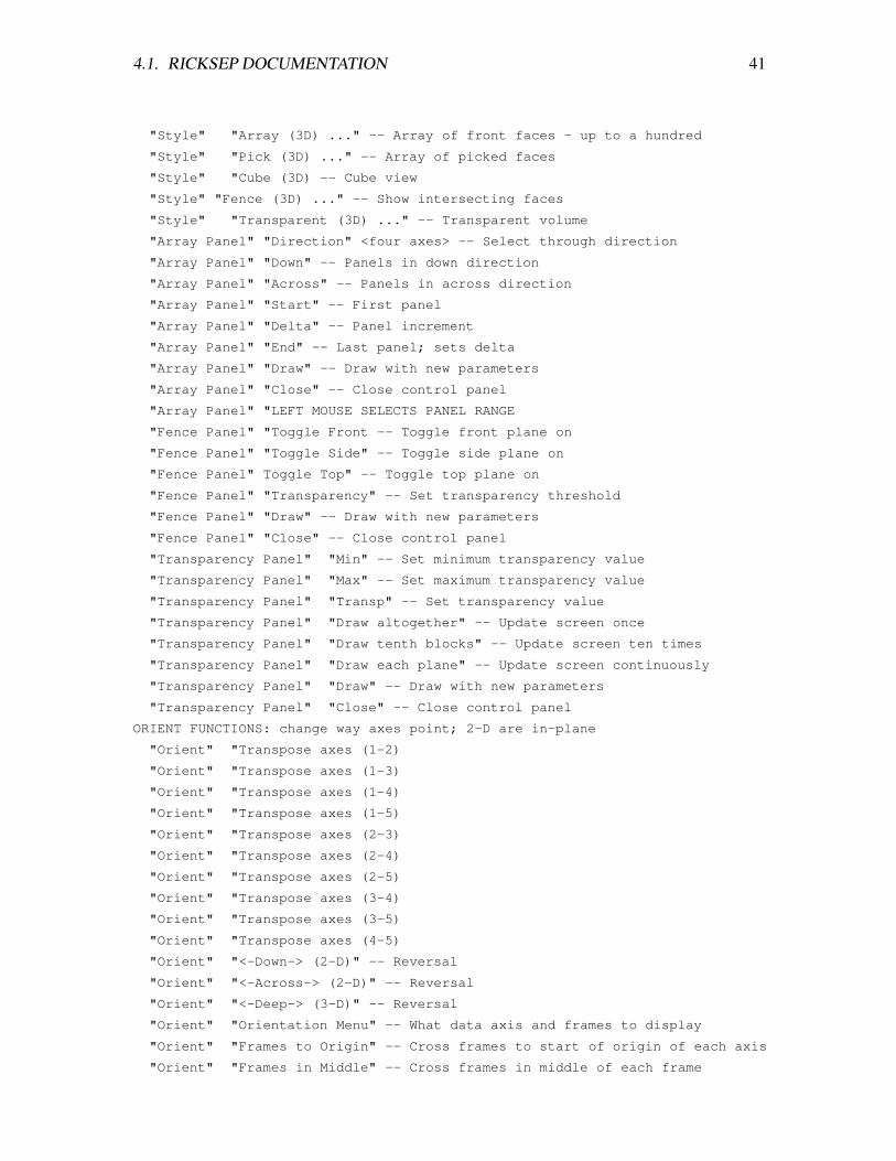
4.1. RICKSEP DOCUMENTATION 41
"Style" "Array (3D) ..." -- Array of front faces - up to a hundred
"Style" "Pick (3D) ..." -- Array of picked faces
"Style" "Cube (3D) -- Cube view
"Style" "Fence (3D) ..." -- Show intersecting faces
"Style" "Transparent (3D) ..." -- Transparent volume
"Array Panel" "Direction" <four axes> -- Select through direction
"Array Panel" "Down" -- Panels in down direction
"Array Panel" "Across" -- Panels in across direction
"Array Panel" "Start" -- First panel
"Array Panel" "Delta" -- Panel increment
"Array Panel" "End" -- Last panel; sets delta
"Array Panel" "Draw" -- Draw with new parameters
"Array Panel" "Close" -- Close control panel
"Array Panel" "LEFT MOUSE SELECTS PANEL RANGE
"Fence Panel" "Toggle Front -- Toggle front plane on
"Fence Panel" "Toggle Side" -- Toggle side plane on
"Fence Panel" Toggle Top" -- Toggle top plane on
"Fence Panel" "Transparency" -- Set transparency threshold
"Fence Panel" "Draw" -- Draw with new parameters
"Fence Panel" "Close" -- Close control panel
"Transparency Panel" "Min" -- Set minimum transparency value
"Transparency Panel" "Max" -- Set maximum transparency value
"Transparency Panel" "Transp" -- Set transparency value
"Transparency Panel" "Draw altogether" -- Update screen once
"Transparency Panel" "Draw tenth blocks" -- Update screen ten times
"Transparency Panel" "Draw each plane" -- Update screen continuously
"Transparency Panel" "Draw" -- Draw with new parameters
"Transparency Panel" "Close" -- Close control panel
ORIENT FUNCTIONS: change way axes point; 2-D are in-plane
"Orient" "Transpose axes (1-2)
"Orient" "Transpose axes (1-3)
"Orient" "Transpose axes (1-4)
"Orient" "Transpose axes (1-5)
"Orient" "Transpose axes (2-3)
"Orient" "Transpose axes (2-4)
"Orient" "Transpose axes (2-5)
"Orient" "Transpose axes (3-4)
"Orient" "Transpose axes (3-5)
"Orient" "Transpose axes (4-5)
"Orient" "<-Down-> (2-D)" -- Reversal
"Orient" "<-Across-> (2-D)" -- Reversal
"Orient" "<-Deep-> (3-D)" -- Reversal
"Orient" "Orientation Menu" -- What data axis and frames to display
"Orient" "Frames to Origin" -- Cross frames to start of origin of each axis
"Orient" "Frames in Middle" -- Cross frames in middle of each frame
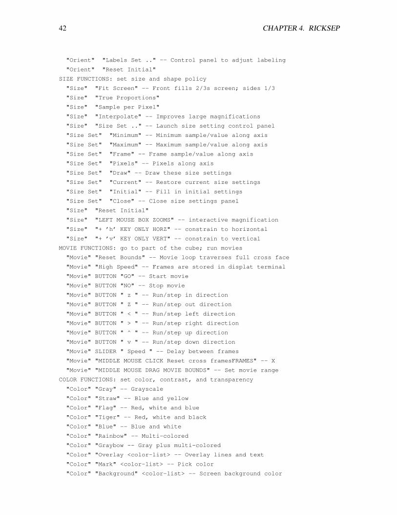
42 CHAPTER 4. RICKSEP
"Orient" "Labels Set .." -- Control panel to adjust labeling
"Orient" "Reset Initial"
SIZE FUNCTIONS: set size and shape policy
"Size" "Fit Screen" -- Front fills 2/3s screen; sides 1/3
"Size" "True Proportions"
"Size" "Sample per Pixel"
"Size" "Interpolate" -- Improves large magnifications
"Size" "Size Set .." -- Launch size setting control panel
"Size Set" "Minimum" -- Minimum sample/value along axis
"Size Set" "Maximum" -- Maximum sample/value along axis
"Size Set" "Frame" -- Frame sample/value along axis
"Size Set" "Pixels" -- Pixels along axis
"Size Set" "Draw" -- Draw these size settings
"Size Set" "Current" -- Restore current size settings
"Size Set" "Initial" -- Fill in initial settings
"Size Set" "Close" -- Close size settings panel
"Size" "Reset Initial"
"Size" "LEFT MOUSE BOX ZOOMS" -- interactive magnification
"Size" "+ ’h’ KEY ONLY HORZ" -- constrain to horizontal
"Size" "+ ’v’ KEY ONLY VERT" -- constrain to vertical
MOVIE FUNCTIONS: go to part of the cube; run movies
"Movie" "Reset Bounds" -- Movie loop traverses full cross face
"Movie" "High Speed" -- Frames are stored in displat terminal
"Movie" BUTTON "GO" -- Start movie
"Movie" BUTTON "NO" -- Stop movie
"Movie" BUTTON " z " -- Run/step in direction
"Movie" BUTTON " Z " -- Run/step out direction
"Movie" BUTTON " < " -- Run/step left direction
"Movie" BUTTON " > " -- Run/step right direction
"Movie" BUTTON " ^ " -- Run/step up direction
"Movie" BUTTON " v " -- Run/step down direction
"Movie" SLIDER " Speed " -- Delay between frames
"Movie" "MIDDLE MOUSE CLICK Reset cross framesFRAMES" -- X
"Movie" "MIDDLE MOUSE DRAG MOVIE BOUNDS" -- Set movie range
COLOR FUNCTIONS: set color, contrast, and transparency
"Color" "Gray" -- Grayscale
"Color" "Straw" -- Blue and yellow
"Color" "Flag" -- Red, white and blue
"Color" "Tiger" -- Red, white and black
"Color" "Blue" -- Blue and white
"Color" "Rainbow" -- Multi-colored
"Color" "Graybow -- Gray plus multi-colored
"Color" "Overlay <color-list> -- Overlay lines and text
"Color" "Mark" <color-list> -- Pick color
"Color" "Background" <color-list> -- Screen background color
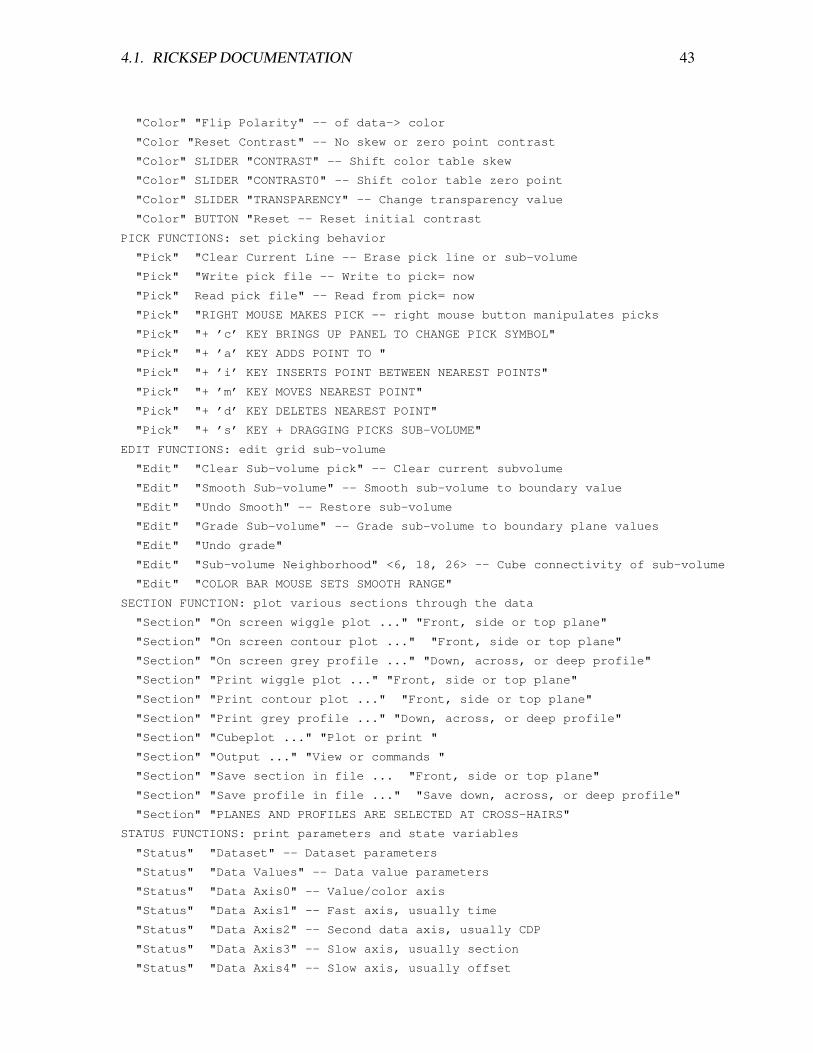
4.1. RICKSEP DOCUMENTATION 43
"Color" "Flip Polarity" -- of data-> color
"Color "Reset Contrast" -- No skew or zero point contrast
"Color" SLIDER "CONTRAST" -- Shift color table skew
"Color" SLIDER "CONTRAST0" -- Shift color table zero point
"Color" SLIDER "TRANSPARENCY" -- Change transparency value
"Color" BUTTON "Reset -- Reset initial contrast
PICK FUNCTIONS: set picking behavior
"Pick" "Clear Current Line -- Erase pick line or sub-volume
"Pick" "Write pick file -- Write to pick= now
"Pick" Read pick file" -- Read from pick= now
"Pick" "RIGHT MOUSE MAKES PICK -- right mouse button manipulates picks
"Pick" "+ ’c’ KEY BRINGS UP PANEL TO CHANGE PICK SYMBOL"
"Pick" "+ ’a’ KEY ADDS POINT TO "
"Pick" "+ ’i’ KEY INSERTS POINT BETWEEN NEAREST POINTS"
"Pick" "+ ’m’ KEY MOVES NEAREST POINT"
"Pick" "+ ’d’ KEY DELETES NEAREST POINT"
"Pick" "+ ’s’ KEY + DRAGGING PICKS SUB-VOLUME"
EDIT FUNCTIONS: edit grid sub-volume
"Edit" "Clear Sub-volume pick" -- Clear current subvolume
"Edit" "Smooth Sub-volume" -- Smooth sub-volume to boundary value
"Edit" "Undo Smooth" -- Restore sub-volume
"Edit" "Grade Sub-volume" -- Grade sub-volume to boundary plane values
"Edit" "Undo grade"
"Edit" "Sub-volume Neighborhood" <6, 18, 26> -- Cube connectivity of sub-volume
"Edit" "COLOR BAR MOUSE SETS SMOOTH RANGE"
SECTION FUNCTION: plot various sections through the data
"Section" "On screen wiggle plot ..." "Front, side or top plane"
"Section" "On screen contour plot ..." "Front, side or top plane"
"Section" "On screen grey profile ..." "Down, across, or deep profile"
"Section" "Print wiggle plot ..." "Front, side or top plane"
"Section" "Print contour plot ..." "Front, side or top plane"
"Section" "Print grey profile ..." "Down, across, or deep profile"
"Section" "Cubeplot ..." "Plot or print "
"Section" "Output ..." "View or commands "
"Section" "Save section in file ... "Front, side or top plane"
"Section" "Save profile in file ..." "Save down, across, or deep profile"
"Section" "PLANES AND PROFILES ARE SELECTED AT CROSS-HAIRS"
STATUS FUNCTIONS: print parameters and state variables
"Status" "Dataset" -- Dataset parameters
"Status" "Data Values" -- Data value parameters
"Status" "Data Axis0" -- Value/color axis
"Status" "Data Axis1" -- Fast axis, usually time
"Status" "Data Axis2" -- Second data axis, usually CDP
"Status" "Data Axis3" -- Slow axis, usually section
"Status" "Data Axis4" -- Slow axis, usually offset
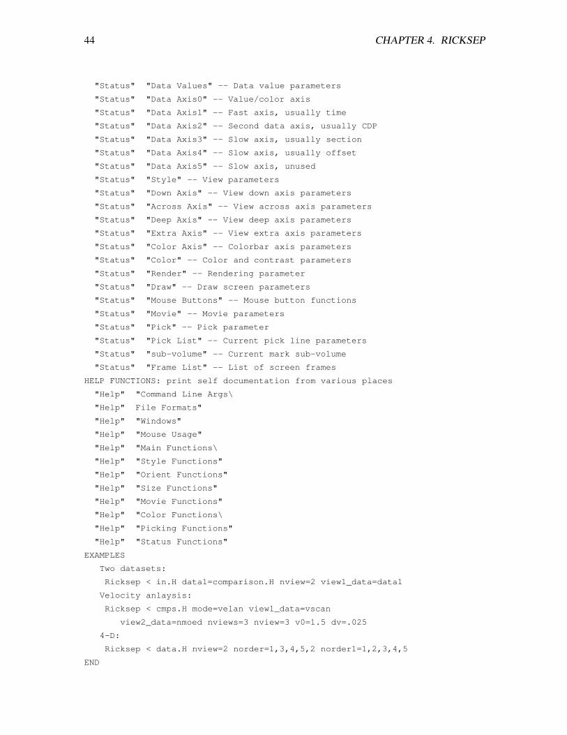
44 CHAPTER 4. RICKSEP
"Status" "Data Values" -- Data value parameters
"Status" "Data Axis0" -- Value/color axis
"Status" "Data Axis1" -- Fast axis, usually time
"Status" "Data Axis2" -- Second data axis, usually CDP
"Status" "Data Axis3" -- Slow axis, usually section
"Status" "Data Axis4" -- Slow axis, usually offset
"Status" "Data Axis5" -- Slow axis, unused
"Status" "Style" -- View parameters
"Status" "Down Axis" -- View down axis parameters
"Status" "Across Axis" -- View across axis parameters
"Status" "Deep Axis" -- View deep axis parameters
"Status" "Extra Axis" -- View extra axis parameters
"Status" "Color Axis" -- Colorbar axis parameters
"Status" "Color" -- Color and contrast parameters
"Status" "Render" -- Rendering parameter
"Status" "Draw" -- Draw screen parameters
"Status" "Mouse Buttons" -- Mouse button functions
"Status" "Movie" -- Movie parameters
"Status" "Pick" -- Pick parameter
"Status" "Pick List" -- Current pick line parameters
"Status" "sub-volume" -- Current mark sub-volume
"Status" "Frame List" -- List of screen frames
HELP FUNCTIONS: print self documentation from various places
"Help" "Command Line Args\
"Help" File Formats"
"Help" "Windows"
"Help" "Mouse Usage"
"Help" "Main Functions\
"Help" "Style Functions"
"Help" "Orient Functions"
"Help" "Size Functions"
"Help" "Movie Functions"
"Help" "Color Functions\
"Help" "Picking Functions"
"Help" "Status Functions"
EXAMPLES
Two datasets:
Ricksep < in.H data1=comparison.H nview=2 view1_data=data1
Velocity anlaysis:
Ricksep < cmps.H mode=velan view1_data=vscan
view2_data=nmoed nviews=3 nview=3 v0=1.5 dv=.025
4-D:
Ricksep < data.H nview=2 norder=1,3,4,5,2 norder1=1,2,3,4,5
END

4.2. EXAMPLES 45
4.2 Examples
This section will demonstrate the use of the Rickmulti and Rickvelan scripts as well as anno-tation and picking in Ricksep. .
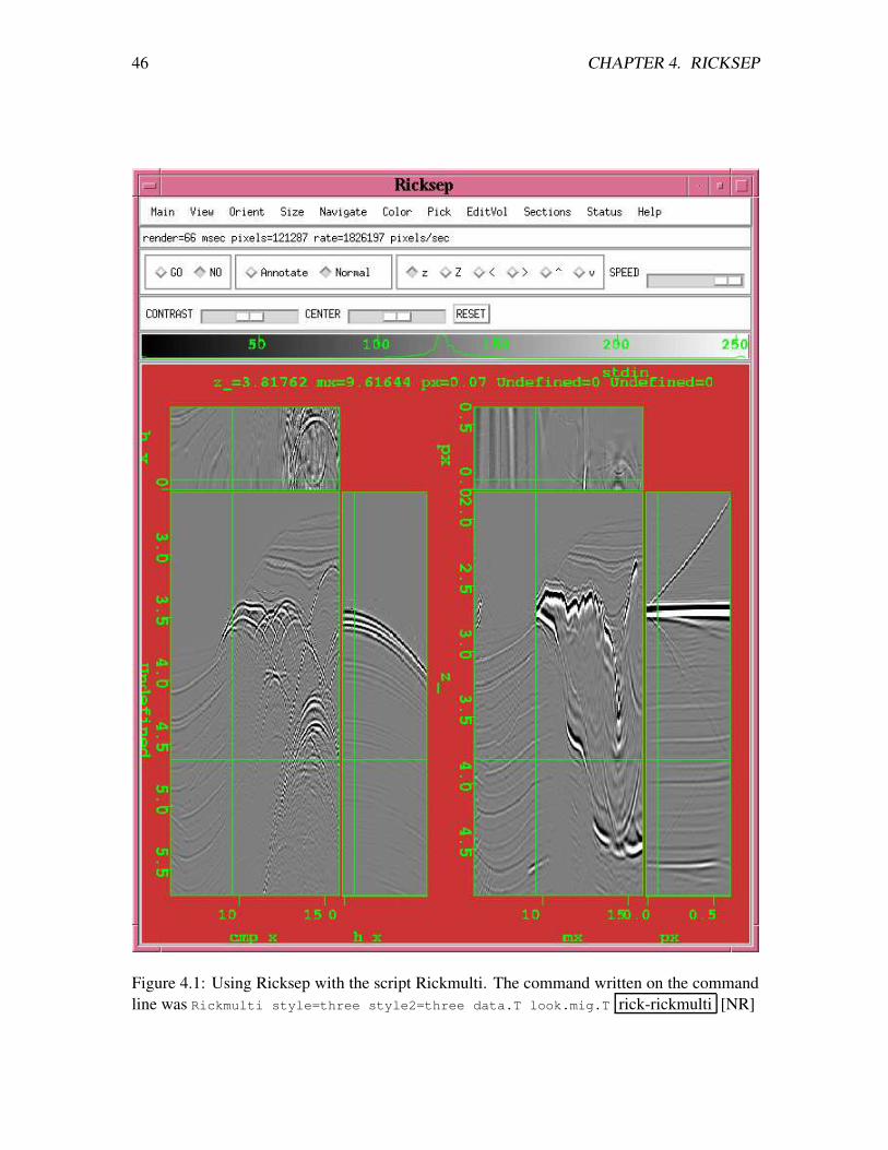
46 CHAPTER 4. RICKSEP
Figure 4.1: Using Ricksep with the script Rickmulti. The command written on the commandline was Rickmulti style=three style2=three data.T look.mig.T rick-rickmulti [NR]
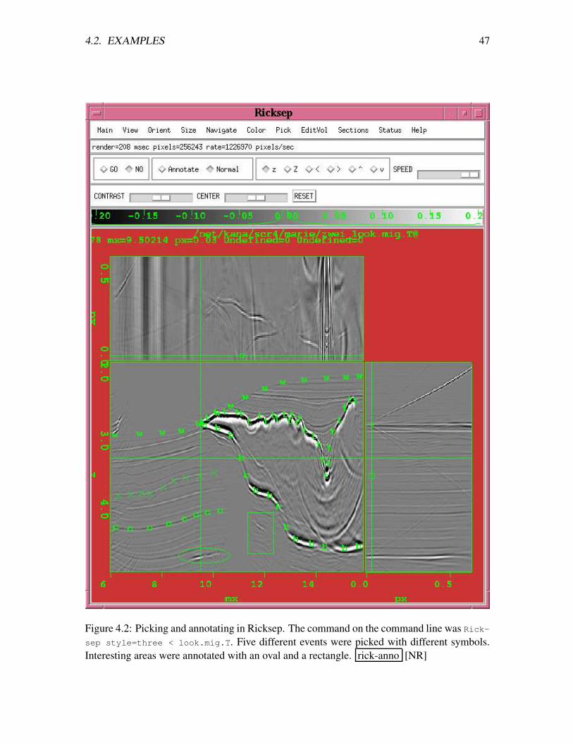
4.2. EXAMPLES 47
Figure 4.2: Picking and annotating in Ricksep. The command on the command line was Rick-sep style=three < look.mig.T. Five different events were picked with different symbols.Interesting areas were annotated with an oval and a rectangle. rick-anno [NR]

48 CHAPTER 4. RICKSEP
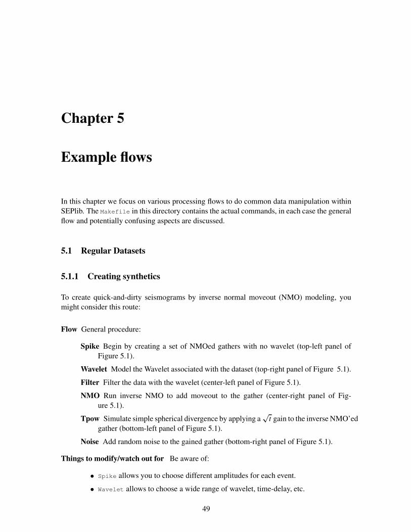
Chapter 5
Example flows
In this chapter we focus on various processing flows to do common data manipulation withinSEPlib. The Makefile in this directory contains the actual commands, in each case the generalflow and potentially confusing aspects are discussed.
5.1 Regular Datasets
5.1.1 Creating synthetics
To create quick-and-dirty seismograms by inverse normal moveout (NMO) modeling, youmight consider this route:
Flow General procedure:
Spike Begin by creating a set of NMOed gathers with no wavelet (top-left panel ofFigure 5.1).
Wavelet Model the Wavelet associated with the dataset (top-right panel of Figure 5.1).
Filter Filter the data with the wavelet (center-left panel of Figure 5.1).
NMO Run inverse NMO to add moveout to the gather (center-right panel of Fig-ure 5.1).
Tpow Simulate simple spherical divergence by applying a√
t gain to the inverse NMO’edgather (bottom-left panel of Figure 5.1).
Noise Add random noise to the gained gather (bottom-right panel of Figure 5.1).
Things to modify/watch out for Be aware of:
• Spike allows you to choose different amplitudes for each event.
• Wavelet allows to choose a wide range of wavelet, time-delay, etc.
49
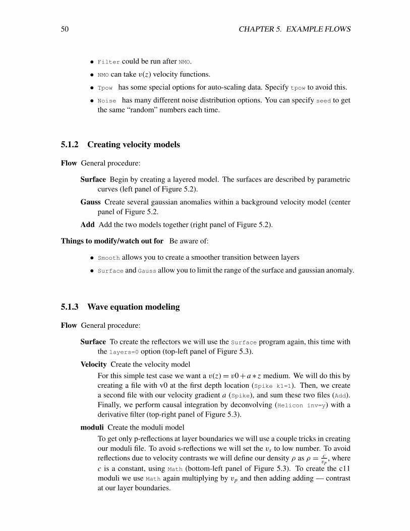
50 CHAPTER 5. EXAMPLE FLOWS
• Filter could be run after NMO.
• NMO can take v(z) velocity functions.
• Tpow has some special options for auto-scaling data. Specify tpow to avoid this.
• Noise has many different noise distribution options. You can specify seed to getthe same “random” numbers each time.
5.1.2 Creating velocity models
Flow General procedure:
Surface Begin by creating a layered model. The surfaces are described by parametriccurves (left panel of Figure 5.2).
Gauss Create several gaussian anomalies within a background velocity model (centerpanel of Figure 5.2.
Add Add the two models together (right panel of Figure 5.2).
Things to modify/watch out for Be aware of:
• Smooth allows you to create a smoother transition between layers
• Surface and Gauss allow you to limit the range of the surface and gaussian anomaly.
5.1.3 Wave equation modeling
Flow General procedure:
Surface To create the reflectors we will use the Surface program again, this time withthe layers=0 option (top-left panel of Figure 5.3).
Velocity Create the velocity modelFor this simple test case we want a v(z)= v0+a ∗ z medium. We will do this bycreating a file with v0 at the first depth location (Spike k1=1). Then, we createa second file with our velocity gradient a (Spike), and sum these two files (Add).Finally, we perform causal integration by deconvolving (Helicon inv=y) with aderivative filter (top-right panel of Figure 5.3).
moduli Create the moduli modelTo get only p-reflections at layer boundaries we will use a couple tricks in creatingour moduli file. To avoid s-reflections we will set the vs to low number. To avoidreflections due to velocity contrasts we will define our density ρ as ρ = c
vp, where
c is a constant, using Math (bottom-left panel of Figure 5.3). To create the c11moduli we use Math again multiplying by vp and then adding adding — contrastat our layer boundaries.
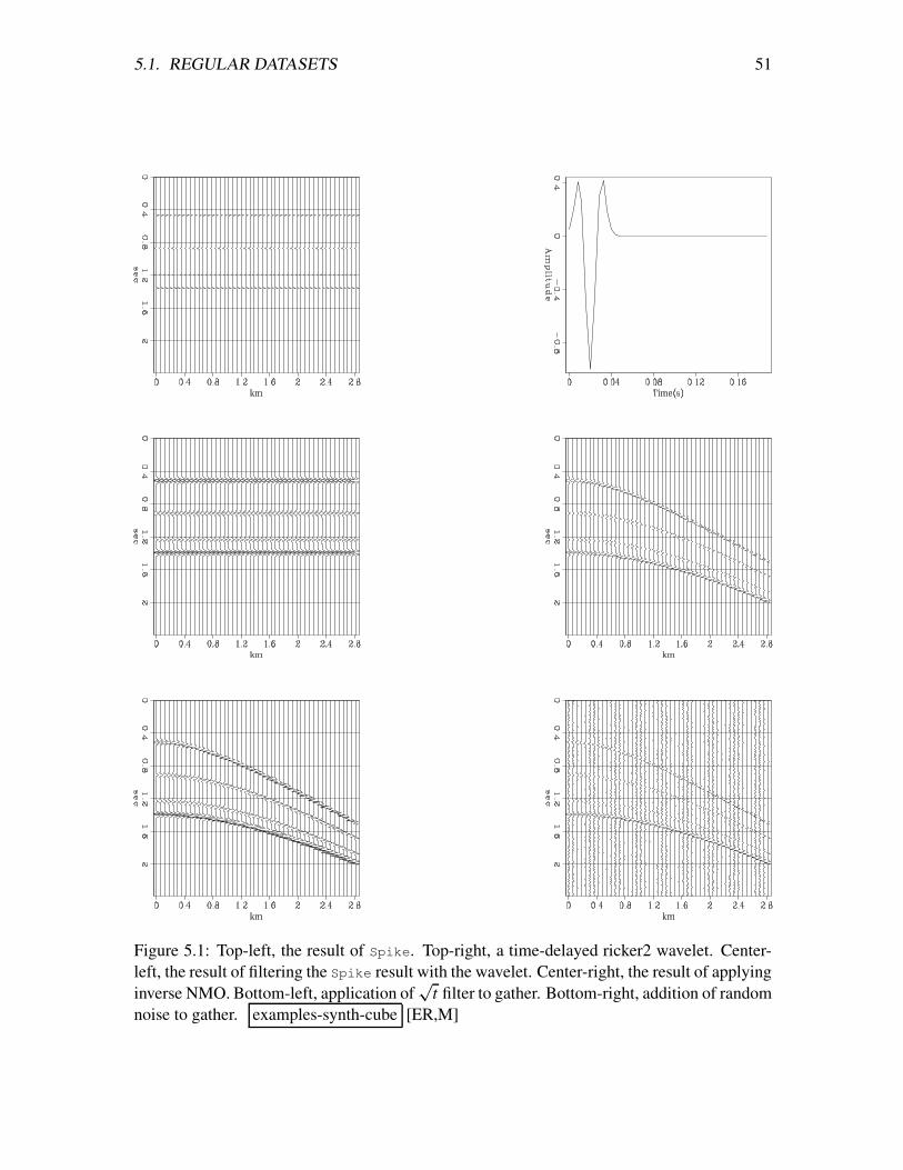
5.1. REGULAR DATASETS 51
Figure 5.1: Top-left, the result of Spike. Top-right, a time-delayed ricker2 wavelet. Center-left, the result of filtering the Spike result with the wavelet. Center-right, the result of applyinginverse NMO. Bottom-left, application of
√t filter to gather. Bottom-right, addition of random
noise to gather. examples-synth-cube [ER,M]
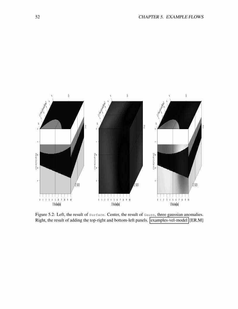
52 CHAPTER 5. EXAMPLE FLOWS
Figure 5.2: Left, the result of Surface. Center, the result of Gauss, three gaussian anomalies.Right, the result of adding the top-right and bottom-left panels. examples-vel-model [ER,M]
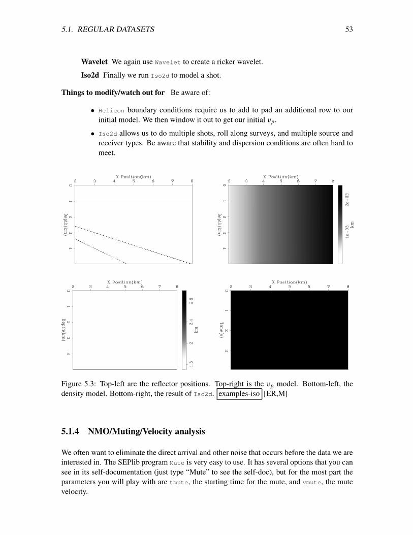
5.1. REGULAR DATASETS 53
Wavelet We again use Wavelet to create a ricker wavelet.
Iso2d Finally we run Iso2d to model a shot.
Things to modify/watch out for Be aware of:
• Helicon boundary conditions require us to add to pad an additional row to ourinitial model. We then window it out to get our initial vp.
• Iso2d allows us to do multiple shots, roll along surveys, and multiple source andreceiver types. Be aware that stability and dispersion conditions are often hard tomeet.
Figure 5.3: Top-left are the reflector positions. Top-right is the vp model. Bottom-left, thedensity model. Bottom-right, the result of Iso2d. examples-iso [ER,M]
5.1.4 NMO/Muting/Velocity analysis
We often want to eliminate the direct arrival and other noise that occurs before the data we areinterested in. The SEPlib program Mute is very easy to use. It has several options that you cansee in its self-documentation (just type “Mute” to see the self-doc), but for the most part theparameters you will play with are tmute, the starting time for the mute, and vmute, the mutevelocity.
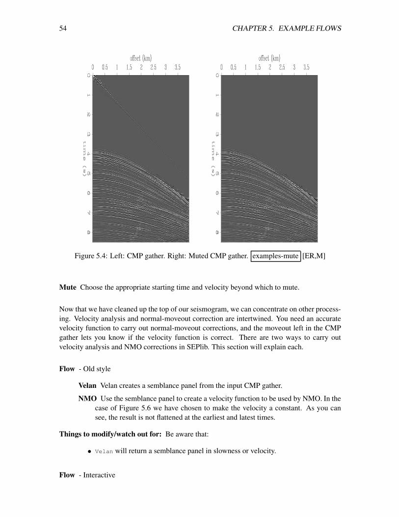
54 CHAPTER 5. EXAMPLE FLOWS
Figure 5.4: Left: CMP gather. Right: Muted CMP gather. examples-mute [ER,M]
Mute Choose the appropriate starting time and velocity beyond which to mute.
Now that we have cleaned up the top of our seismogram, we can concentrate on other process-ing. Velocity analysis and normal-moveout correction are intertwined. You need an accuratevelocity function to carry out normal-moveout corrections, and the moveout left in the CMPgather lets you know if the velocity function is correct. There are two ways to carry outvelocity analysis and NMO corrections in SEPlib. This section will explain each.
Flow - Old style
Velan Velan creates a semblance panel from the input CMP gather.
NMO Use the semblance panel to create a velocity function to be used by NMO. In thecase of Figure 5.6 we have chosen to make the velocity a constant. As you cansee, the result is not flattened at the earliest and latest times.
Things to modify/watch out for: Be aware that:
• Velan will return a semblance panel in slowness or velocity.
Flow - Interactive
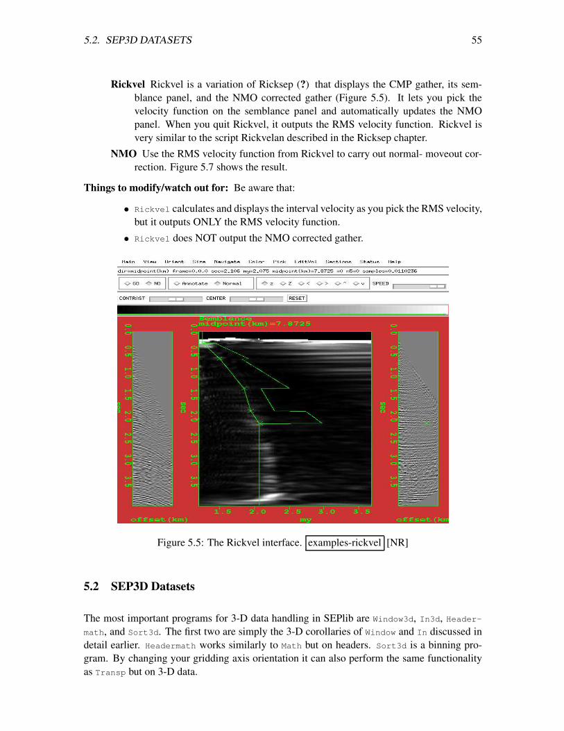
5.2. SEP3D DATASETS 55
Rickvel Rickvel is a variation of Ricksep (?) that displays the CMP gather, its sem-blance panel, and the NMO corrected gather (Figure 5.5). It lets you pick thevelocity function on the semblance panel and automatically updates the NMOpanel. When you quit Rickvel, it outputs the RMS velocity function. Rickvel isvery similar to the script Rickvelan described in the Ricksep chapter.
NMO Use the RMS velocity function from Rickvel to carry out normal- moveout cor-rection. Figure 5.7 shows the result.
Things to modify/watch out for: Be aware that:
• Rickvel calculates and displays the interval velocity as you pick the RMS velocity,but it outputs ONLY the RMS velocity function.• Rickvel does NOT output the NMO corrected gather.
Figure 5.5: The Rickvel interface. examples-rickvel [NR]
5.2 SEP3D Datasets
The most important programs for 3-D data handling in SEPlib are Window3d, In3d, Header-math, and Sort3d. The first two are simply the 3-D corollaries of Window and In discussed indetail earlier. Headermath works similarly to Math but on headers. Sort3d is a binning pro-gram. By changing your gridding axis orientation it can also perform the same functionalityas Transp but on 3-D data.
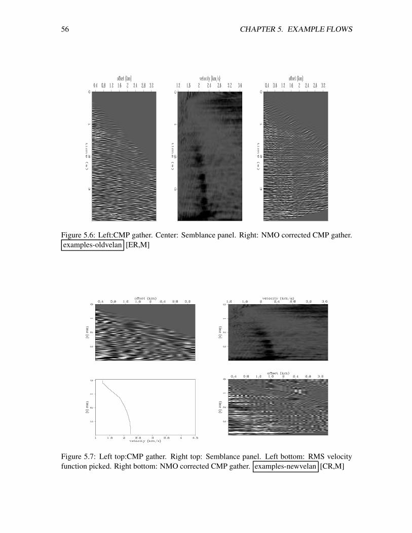
56 CHAPTER 5. EXAMPLE FLOWS
Figure 5.6: Left:CMP gather. Center: Semblance panel. Right: NMO corrected CMP gather.examples-oldvelan [ER,M]
Figure 5.7: Left top:CMP gather. Right top: Semblance panel. Left bottom: RMS velocityfunction picked. Right bottom: NMO corrected CMP gather. examples-newvelan [CR,M]
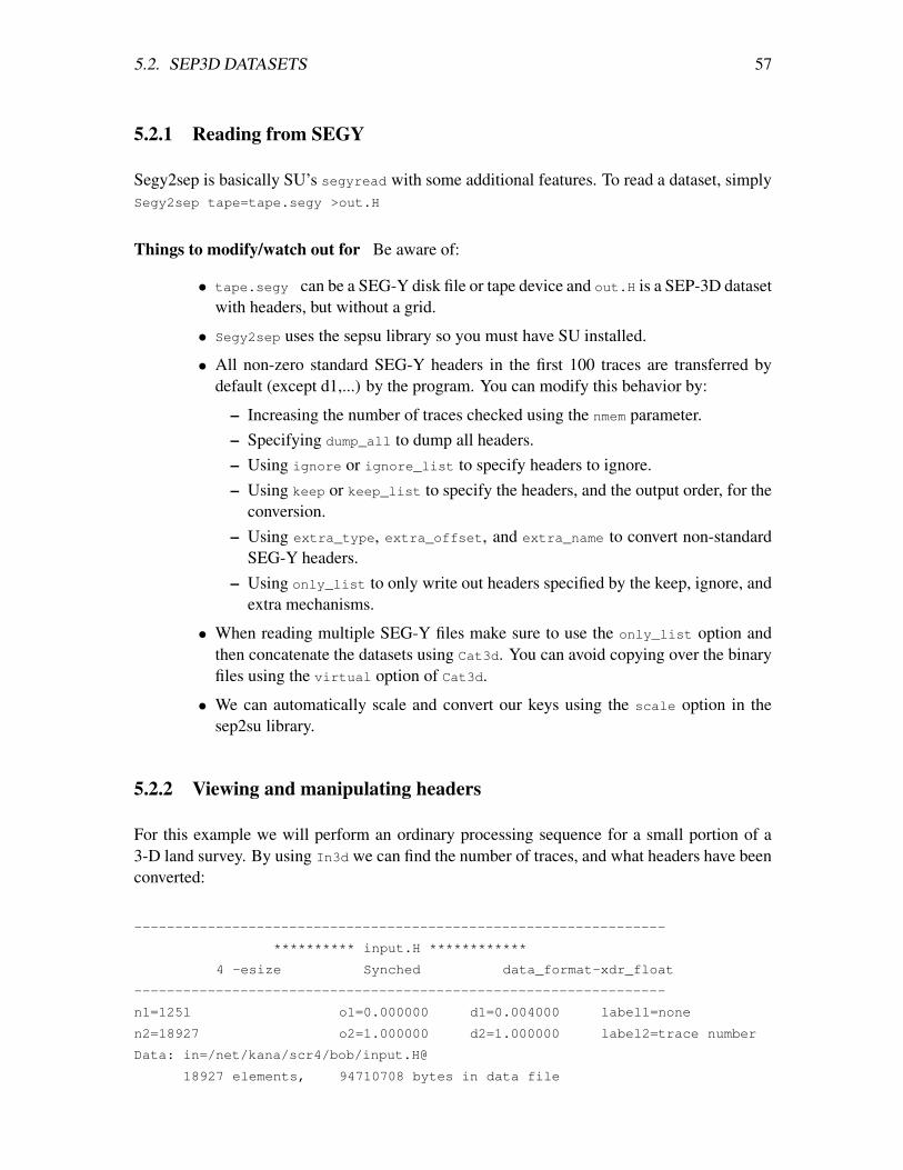
5.2. SEP3D DATASETS 57
5.2.1 Reading from SEGY
Segy2sep is basically SU’s segyread with some additional features. To read a dataset, simplySegy2sep tape=tape.segy >out.H
Things to modify/watch out for Be aware of:
• tape.segy can be a SEG-Y disk file or tape device and out.H is a SEP-3D datasetwith headers, but without a grid.
• Segy2sep uses the sepsu library so you must have SU installed.
• All non-zero standard SEG-Y headers in the first 100 traces are transferred bydefault (except d1,...) by the program. You can modify this behavior by:
– Increasing the number of traces checked using the nmem parameter.– Specifying dump_all to dump all headers.– Using ignore or ignore_list to specify headers to ignore.– Using keep or keep_list to specify the headers, and the output order, for the
conversion.– Using extra_type, extra_offset, and extra_name to convert non-standard
SEG-Y headers.– Using only_list to only write out headers specified by the keep, ignore, and
extra mechanisms.
• When reading multiple SEG-Y files make sure to use the only_list option andthen concatenate the datasets using Cat3d. You can avoid copying over the binaryfiles using the virtual option of Cat3d.
• We can automatically scale and convert our keys using the scale option in thesep2su library.
5.2.2 Viewing and manipulating headers
For this example we will perform an ordinary processing sequence for a small portion of a3-D land survey. By using In3d we can find the number of traces, and what headers have beenconverted:
-----------------------------------------------------------------
********** input.H ************
4 -esize Synched data_format-xdr_float
-----------------------------------------------------------------
n1=1251 o1=0.000000 d1=0.004000 label1=none
n2=18927 o2=1.000000 d2=1.000000 label2=trace number
Data: in=/net/kana/scr4/bob/input.H@
18927 elements, 94710708 bytes in data file
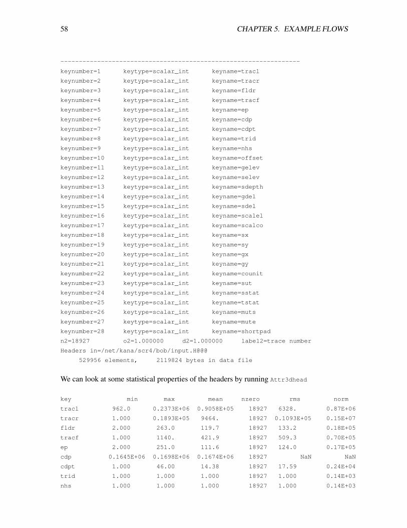
58 CHAPTER 5. EXAMPLE FLOWS
-----------------------------------------------------------------
keynumber=1 keytype=scalar_int keyname=tracl
keynumber=2 keytype=scalar_int keyname=tracr
keynumber=3 keytype=scalar_int keyname=fldr
keynumber=4 keytype=scalar_int keyname=tracf
keynumber=5 keytype=scalar_int keyname=ep
keynumber=6 keytype=scalar_int keyname=cdp
keynumber=7 keytype=scalar_int keyname=cdpt
keynumber=8 keytype=scalar_int keyname=trid
keynumber=9 keytype=scalar_int keyname=nhs
keynumber=10 keytype=scalar_int keyname=offset
keynumber=11 keytype=scalar_int keyname=gelev
keynumber=12 keytype=scalar_int keyname=selev
keynumber=13 keytype=scalar_int keyname=sdepth
keynumber=14 keytype=scalar_int keyname=gdel
keynumber=15 keytype=scalar_int keyname=sdel
keynumber=16 keytype=scalar_int keyname=scalel
keynumber=17 keytype=scalar_int keyname=scalco
keynumber=18 keytype=scalar_int keyname=sx
keynumber=19 keytype=scalar_int keyname=sy
keynumber=20 keytype=scalar_int keyname=gx
keynumber=21 keytype=scalar_int keyname=gy
keynumber=22 keytype=scalar_int keyname=counit
keynumber=23 keytype=scalar_int keyname=sut
keynumber=24 keytype=scalar_int keyname=sstat
keynumber=25 keytype=scalar_int keyname=tstat
keynumber=26 keytype=scalar_int keyname=muts
keynumber=27 keytype=scalar_int keyname=mute
keynumber=28 keytype=scalar_int keyname=shortpad
n2=18927 o2=1.000000 d2=1.000000 label2=trace number
Headers in=/net/kana/scr4/bob/input.H@@@
529956 elements, 2119824 bytes in data file
We can look at some statistical properties of the headers by running Attr3dhead
key min max mean nzero rms norm
tracl 962.0 0.2373E+06 0.9058E+05 18927 6328. 0.87E+06
tracr 1.000 0.1893E+05 9464. 18927 0.1093E+05 0.15E+07
fldr 2.000 263.0 119.7 18927 133.2 0.18E+05
tracf 1.000 1140. 421.9 18927 509.3 0.70E+05
ep 2.000 251.0 111.6 18927 124.0 0.17E+05
cdp 0.1645E+06 0.1698E+06 0.1674E+06 18927 NaN NaN
cdpt 1.000 46.00 14.38 18927 17.59 0.24E+04
trid 1.000 1.000 1.000 18927 1.000 0.14E+03
nhs 1.000 1.000 1.000 18927 1.000 0.14E+03
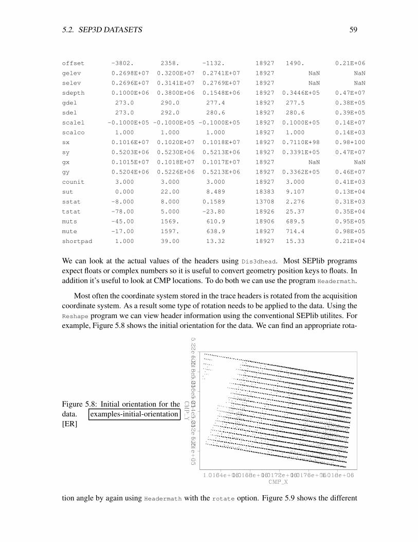
5.2. SEP3D DATASETS 59
offset -3802. 2358. -1132. 18927 1490. 0.21E+06
gelev 0.2698E+07 0.3200E+07 0.2741E+07 18927 NaN NaN
selev 0.2696E+07 0.3141E+07 0.2769E+07 18927 NaN NaN
sdepth 0.1000E+06 0.3800E+06 0.1548E+06 18927 0.3446E+05 0.47E+07
gdel 273.0 290.0 277.4 18927 277.5 0.38E+05
sdel 273.0 292.0 280.6 18927 280.6 0.39E+05
scalel -0.1000E+05 -0.1000E+05 -0.1000E+05 18927 0.1000E+05 0.14E+07
scalco 1.000 1.000 1.000 18927 1.000 0.14E+03
sx 0.1016E+07 0.1020E+07 0.1018E+07 18927 0.7110E+98 0.98+100
sy 0.5203E+06 0.5230E+06 0.5213E+06 18927 0.3391E+05 0.47E+07
gx 0.1015E+07 0.1018E+07 0.1017E+07 18927 NaN NaN
gy 0.5204E+06 0.5226E+06 0.5213E+06 18927 0.3362E+05 0.46E+07
counit 3.000 3.000 3.000 18927 3.000 0.41E+03
sut 0.000 22.00 8.489 18383 9.107 0.13E+04
sstat -8.000 8.000 0.1589 13708 2.276 0.31E+03
tstat -78.00 5.000 -23.80 18926 25.37 0.35E+04
muts -45.00 1569. 610.9 18906 689.5 0.95E+05
mute -17.00 1597. 638.9 18927 714.4 0.98E+05
shortpad 1.000 39.00 13.32 18927 15.33 0.21E+04
We can look at the actual values of the headers using Dis3dhead. Most SEPlib programsexpect floats or complex numbers so it is useful to convert geometry position keys to floats. Inaddition it’s useful to look at CMP locations. To do both we can use the program Headermath.
Most often the coordinate system stored in the trace headers is rotated from the acquisitioncoordinate system. As a result some type of rotation needs to be applied to the data. Using theReshape program we can view header information using the conventional SEPlib utilites. Forexample, Figure 5.8 shows the initial orientation for the data. We can find an appropriate rota-
Figure 5.8: Initial orientation for thedata. examples-initial-orientation[ER]
tion angle by again using Headermath with the rotate option. Figure 5.9 shows the different
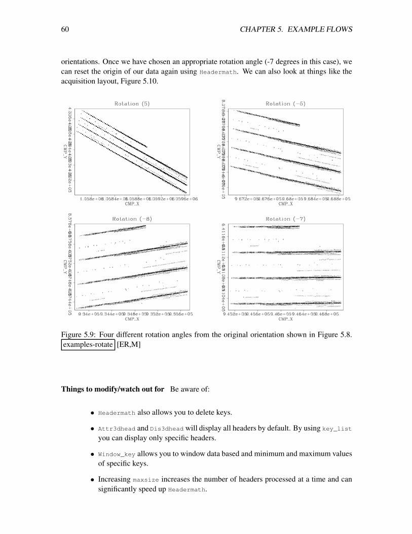
60 CHAPTER 5. EXAMPLE FLOWS
orientations. Once we have chosen an appropriate rotation angle (-7 degrees in this case), wecan reset the origin of our data again using Headermath. We can also look at things like theacquisition layout, Figure 5.10.
Figure 5.9: Four different rotation angles from the original orientation shown in Figure 5.8.examples-rotate [ER,M]
Things to modify/watch out for Be aware of:
• Headermath also allows you to delete keys.
• Attr3dhead and Dis3dhead will display all headers by default. By using key_list
you can display only specific headers.
• Window_key allows you to window data based and minimum and maximum valuesof specific keys.
• Increasing maxsize increases the number of headers processed at a time and cansignificantly speed up Headermath.
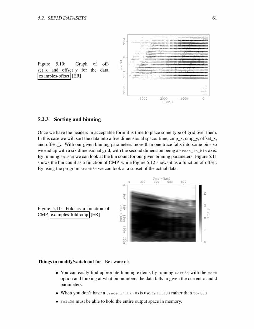
5.2. SEP3D DATASETS 61
Figure 5.10: Graph of off-set_x and offset_y for the data.examples-offset [ER]
5.2.3 Sorting and binning
Once we have the headers in acceptable form it is time to place some type of grid over them.In this case we will sort the data into a five dimensional space: time, cmp_x, cmp_y, offset_x,and offset_y. With our given binning parameters more than one trace falls into some bins sowe end up with a six dimensional grid, with the second dimension being a trace_in_bin axis.By running Fold3d we can look at the bin count for our given binning parameters. Figure 5.11shows the bin count as a function of CMP, while Figure 5.12 shows it as a function of offset.By using the program Stack3d we can look at a subset of the actual data.
Figure 5.11: Fold as a function ofCMP. examples-fold-cmp [ER]
Things to modify/watch out for Be aware of:
• You can easily find approriate binning extents by running Sort3d with the verb
option and looking at what bin numbers the data falls in given the current o and dparameters.
• When you don’t have a trace_in_bin axis use Infill3d rather than Sort3d
• Fold3d must be able to hold the entire output space in memory.
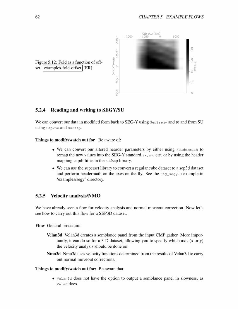
62 CHAPTER 5. EXAMPLE FLOWS
Figure 5.12: Fold as a function of off-set. examples-fold-offset [ER]
5.2.4 Reading and writing to SEGY/SU
We can convert our data in modified form back to SEG-Y using Sep2segy and to and from SUusing Sep2su and Su2sep.
Things to modify/watch out for Be aware of:
• We can convert our altered hearder parameters by either using Headermath toremap the new values into the SEG-Y standard sx, sy, etc. or by using the headermapping capibilities in the su2sep library.
• We can use the superset library to convert a regular cube dataset to a sep3d datasetand perform headermath on the axes on the fly. See the reg_segy.H example in‘examples/segy’ directory.
5.2.5 Velocity analysis/NMO
We have already seen a flow for velocity analysis and normal moveout correction. Now let’ssee how to carry out this flow for a SEP3D dataset.
Flow General procedure:
Velan3d Velan3d creates a semblance panel from the input CMP gather. More impor-tantly, it can do so for a 3-D dataset, allowing you to specify which axis (x or y)the velocity analysis should be done on.
Nmo3d Nmo3d uses velocity functions determined from the results of Velan3d to carryout normal moveout corrections.
Things to modify/watch out for: Be aware that:
• Velan3d does not have the option to output a semblance panel in slowness, asVelan does.
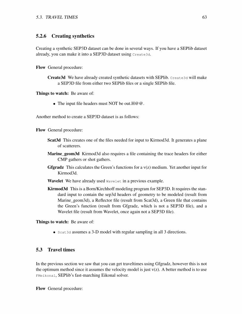
5.3. TRAVEL TIMES 63
5.2.6 Creating synthetics
Creating a synthetic SEP3D dataset can be done in several ways. If you have a SEPlib datasetalready, you can make it into a SEP3D dataset using Create3d.
Flow General procedure:
Create3d We have already created synthetic datasets with SEPlib. Create3d will makea SEP3D file from either two SEPlib files or a single SEPlib file.
Things to watch: Be aware of:
• The input file headers must NOT be out.H@@.
Another method to create a SEP3D dataset is as follows:
Flow General procedure:
Scat3d This creates one of the files needed for input to Kirmod3d. It generates a planeof scatterers.
Marine_geom3d Kirmod3d also requires a file containing the trace headers for eitherCMP gathers or shot gathers.
Gfgradz This calculates the Green’s functions for a v(z) medium. Yet another input forKirmod3d.
Wavelet We have already used Wavelet in a previous example.
Kirmod3d This is a Born/Kirchhoff modeling program for SEP3D. It requires the stan-dard input to contain the sep3d headers of geometry to be modeled (result fromMarine_geom3d), a Reflector file (result from Scat3d), a Green file that containsthe Green’s function (result from Gfgradz, which is not a SEP3D file), and aWavelet file (result from Wavelet, once again not a SEP3D file).
Things to watch: Be aware of:
• Scat3d assumes a 3-D model with regular sampling in all 3 directions.
5.3 Travel times
In the previous section we saw that you can get traveltimes using Gfgradz, however this is notthe optimum method since it assumes the velocity model is just v(z). A better method is to useFMeikonal, SEPlib’s fast-marching Eikonal solver.
Flow General procedure:
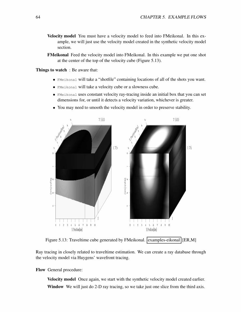
64 CHAPTER 5. EXAMPLE FLOWS
Velocity model You must have a velocity model to feed into FMeikonal. In this ex-ample, we will just use the velocity model created in the synthetic velocity modelsection.
FMeikonal Feed the velocity model into FMeikonal. In this example we put one shotat the center of the top of the velocity cube (Figure 5.13).
Things to watch : Be aware that:
• FMeikonal will take a “shotfile” containing locations of all of the shots you want.
• FMeikonal will take a velocity cube or a slowness cube.
• FMeikonal uses constant velocity ray-tracing inside an initial box that you can setdimensions for, or until it detects a velocity variation, whichever is greater.
• You may need to smooth the velocity model in order to preserve stability.
Figure 5.13: Traveltime cube generated by FMeikonal. examples-eikonal [ER,M]
Ray tracing in closely related to traveltime estimation. We can create a ray database throughthe velocity model via Huygens’ wavefront tracing.
Flow General procedure:
Velocity model Once again, we start with the synthetic velocity model created earlier.
Window We will just do 2-D ray tracing, so we take just one slice from the third axis.
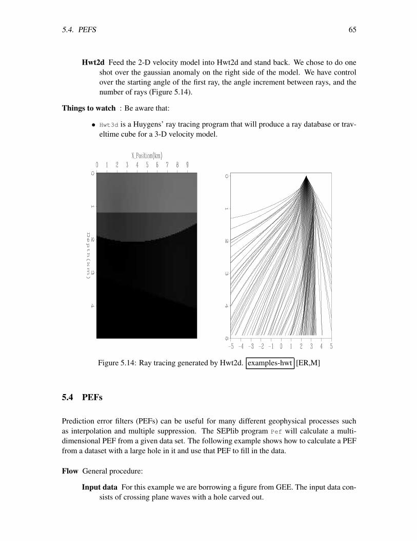
5.4. PEFS 65
Hwt2d Feed the 2-D velocity model into Hwt2d and stand back. We chose to do oneshot over the gaussian anomaly on the right side of the model. We have controlover the starting angle of the first ray, the angle increment between rays, and thenumber of rays (Figure 5.14).
Things to watch : Be aware that:
• Hwt3d is a Huygens’ ray tracing program that will produce a ray database or trav-eltime cube for a 3-D velocity model.
Figure 5.14: Ray tracing generated by Hwt2d. examples-hwt [ER,M]
5.4 PEFs
Prediction error filters (PEFs) can be useful for many different geophysical processes suchas interpolation and multiple suppression. The SEPlib program Pef will calculate a multi-dimensional PEF from a given data set. The following example shows how to calculate a PEFfrom a dataset with a large hole in it and use that PEF to fill in the data.
Flow General procedure:
Input data For this example we are borrowing a figure from GEE. The input data con-sists of crossing plane waves with a hole carved out.
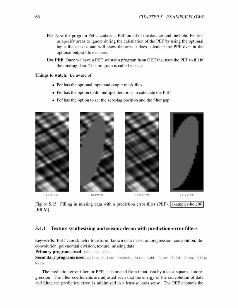
66 CHAPTER 5. EXAMPLE FLOWS
Pef Now the program Pef calculates a PEF on all of the data around the hole. Pef letsus specify areas to ignore during the calculation of the PEF by using the optionalinput file maskin and will show the area it does calculate the PEF over in theoptional output file maskout.
Use PEF Once we have a PEF, we use a program from GEE that uses the PEF to fill inthe missing data. This program is called Miss.x.
Things to watch: Be aware of:
• Pef has the optional input and output mask files.
• Pef has the option to do multiple iterations to calculate the PEF.
• Pef has the option to set the zero-lag position and the filter gap.
Figure 5.15: Filling in missing data with a prediction error filter (PEF). examples-hole90[ER,M]
5.4.1 Texture synthesizing and seismic decon with prediction-error filters
keywords: PEF, causal, helix transform, known data mask, autoregression, convolution, de-convolution, polynomial division, texture, missing data.Primary programs used: Pef, Helicon
Secondary programs used: Spike, Noise, Smooth, Attr, Add, Rtoc, Ft3d, Cabs, Clip,
Math.
The prediction-error filter, or PEF, is estimated from input data by a least-squares autore-gression. The filter coefficients are adjusted such that the energy of the convolution of dataand filter, the prediction error, is minimized in a least-squares sense. The PEF captures the
5.4. PEFS 67
gross spectral qualities of the data from which it was estimated. The PEF discussed here iscausal, with a fixed “1” at zero lag. To learn about the concept of causality in more than onedimension, see (cite GEE).
SEPlib program Pef utilizes the Helix transform (cite) to estimate an n-dimensional PEFfrom data of dimension ≥ n. A main advantage of PEF-based techniques over other spectraltechniques occurs when some data is missing. Pef handles missing data through the use ofa user-supplied known data mask. Special care must be taken to ensure that enough datais present to estimate a PEF. To understand which data contributes to the PEF estimation,imagine that a filter-shaped template is slid around the gridded data. Only at places where allcoefficients of the template fall on known data does Pef use the data in the estimation. Pef
outputs a “output filter mask”, computed from the known data mask, which illustrates whichdata was used in the inversion.
Once a PEF has been estimated, SEPlib program Helicon can apply convolution or inverseconvolution (deconvolution) to n-dimensional data, assuming the PEF is of dimension ≤ n.The deconvolution operation is implemented as polynomial division (cite).
Flow 1-D PEF estimation and seismic decon - General procedure:
Make a 1-D synthetic First look at this command: Spike n1=64 k1=-1 | Noise type=1
seed=13891 | Smooth rect1=3 > 0.H
It uses Spike to create a 1-D cube with 64 samples, all zeros. Noise makes randomnoise. The seed parameter ensures that we get the same “random” numbers eachtime we regenerate the data. Finally, Smooth smoothes out the random numbersinto something more predictable.We would prefer that our synthetic data be zero-mean. We could use Attr to com-pute the mean, then use Add, with a hard-coded makerule to subtract the meanvalue. However, we will use some trickery to do this automatically. Look at thiscommand:< 0.H Add scale=-1 | Add add=‘< 0.H Attr param=1 | Get parform=n mean-
val‘ | Add scale=-1 > rand1d.H
First we scale 0.H by -1. Then we play a shell script trick, using the Attr com-mand, to extract the mean value from 0.H, and then Add to add the mean valueback to 0.H. Last, we scale the result by -1. The random data is displayed in thetop panel of Figure 5.16.
View the data’s spectrum The second panel of Figure 5.16 shows the spectrum of thesmoothed-random input data. It was made by the following command:< rand1d.H Rtoc | Ft3d sign1=-1.0 center1=1.0 | Cabs > ispc.H
Rtoc creates a dummy complex-valued dataset using rand1d.H, where the realpart is rand1d.H and the imaginary part is zero. Ft3d is a general purpose FourierTransform program. Cabs can compute the power spectrum of the FT’ed data:“data*conjugate(data)”.
Estimate a 1-D PEF From the input data (top panel of Figure 5.16), we can estimate aone-dimensional PEF with the following command:
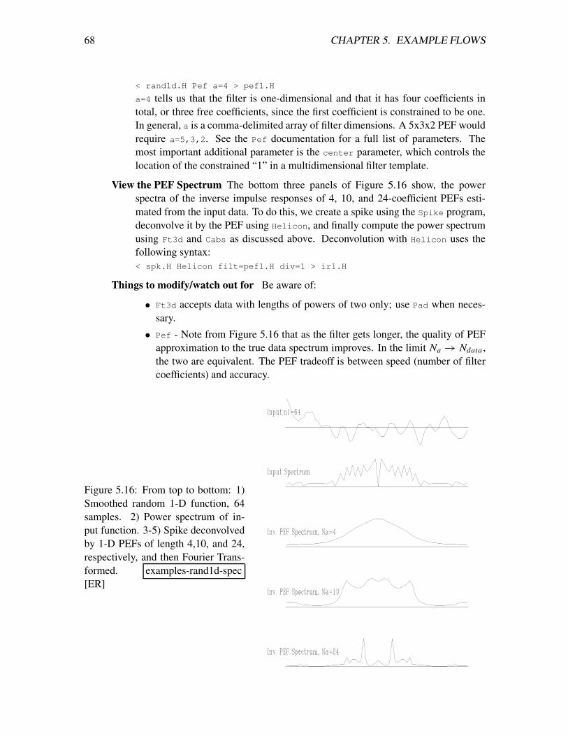
68 CHAPTER 5. EXAMPLE FLOWS
< rand1d.H Pef a=4 > pef1.H
a=4 tells us that the filter is one-dimensional and that it has four coefficients intotal, or three free coefficients, since the first coefficient is constrained to be one.In general, a is a comma-delimited array of filter dimensions. A 5x3x2 PEF wouldrequire a=5,3,2. See the Pef documentation for a full list of parameters. Themost important additional parameter is the center parameter, which controls thelocation of the constrained “1” in a multidimensional filter template.
View the PEF Spectrum The bottom three panels of Figure 5.16 show, the powerspectra of the inverse impulse responses of 4, 10, and 24-coefficient PEFs esti-mated from the input data. To do this, we create a spike using the Spike program,deconvolve it by the PEF using Helicon, and finally compute the power spectrumusing Ft3d and Cabs as discussed above. Deconvolution with Helicon uses thefollowing syntax:< spk.H Helicon filt=pef1.H div=1 > ir1.H
Things to modify/watch out for Be aware of:
• Ft3d accepts data with lengths of powers of two only; use Pad when neces-sary.
• Pef - Note from Figure 5.16 that as the filter gets longer, the quality of PEFapproximation to the true data spectrum improves. In the limit Na → Ndata ,the two are equivalent. The PEF tradeoff is between speed (number of filtercoefficients) and accuracy.
Figure 5.16: From top to bottom: 1)Smoothed random 1-D function, 64samples. 2) Power spectrum of in-put function. 3-5) Spike deconvolvedby 1-D PEFs of length 4,10, and 24,respectively, and then Fourier Trans-formed. examples-rand1d-spec[ER]
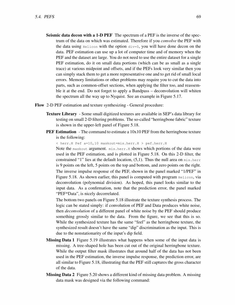
5.4. PEFS 69
Seismic data decon with a 1-D PEF The spectrum of a PEF is the inverse of the spec-trum of the data on which was estimated. Therefore if you convolve the PEF withthe data using Helicon with the option div=0, you will have done decon on thedata. PEF estimation can use up a lot of computer time and of memory when thePEF and the dataset are large. You do not need to use the entire dataset for a singlePEF estimation, do it on small data portions (which can be as small as a singletrace) at various midpoint and offsets, and if the PEFs look very similar then youcan simply stack them to get a more representative one and to get rid of small localerrors. Memory limitations or other problems may require you to cut the data intoparts, such as common-offset sections, when applying the filter too, and reassem-ble it at the end. Do not forget to apply a Bandpass – deconvolution will whitenthe spectrum all the way up to Nyquist. See an example in Figure 5.17.
Flow 2-D PEF estimation and texture synthesizing - General procedure:
Texture Library - Some small digitized textures are available in SEP’s data library fortesting on small 2-D filtering problems. The so-called “herringbone fabric” textureis shown in the upper-left panel of Figure 5.18.
PEF Estimation - The command to estimate a 10x10 PEF from the herringbone textureis the following:< herr.H Pef a=10,10 maskout=mis.herr.H > pef.herr.H
Note the maskout argument. mis.herr.H shows which portions of the data wereused in the PEF estimation, and is plotted in Figure 5.18. On this 2-D filter, theconstrained “1” lies at the default location, (5,1). Thus the null area on mis.herr
is 9 points on the left, 5 points on the top and bottom, and zero points on the right.The inverse impulse response of the PEF, shown in the panel marked “1/PEF” inFigure 5.18. As shown earlier, this panel is computed with program Helicon, viadeconvolution (polynomial division). As hoped, this panel looks similar to theinput data. As a confirmation, note that the prediction error, the panel marked“PEF*Data”, is nicely decorrelated.The bottom two panels on Figure 5.18 illustrate the texture synthesis process. Thelogic can be stated simply: if convolution of PEF and Data produces white noise,then deconvolution of a different panel of white noise by the PEF should producesomething grossly similar to the data. From the figure, we see that this is so.While the synthesized texture has the same “feel” as the herringbone texture, thesynthesized result doesn’t have the same “dip” discrimination as the input. This isdue to the nonstationarity of the input’s dip field.
Missing Data 1 Figure 5.19 illustrates what happens when some of the input data ismissing. A tree-shaped hole has been cut out of the original herringbone texture.While the output filter mask illustrates that around half of the data has not beenused in the PEF estimation, the inverse impulse response, the prediction error, areall similar to Figure 5.18, illustrating that the PEF still captures the gross characterof the data.
Missing Data 2 Figure 5.20 shows a different kind of missing data problem. A missingdata mask was designed via the following command:
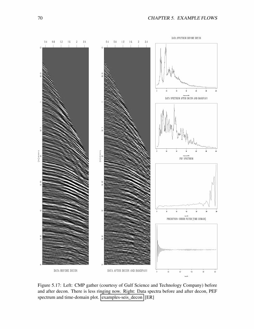
70 CHAPTER 5. EXAMPLE FLOWS
Figure 5.17: Left: CMP gather (courtesy of Gulf Science and Technology Company) beforeand after decon. There is less ringing now. Right: Data spectra before and after decon, PEFspectrum and time-domain plot. examples-seis_decon [ER]
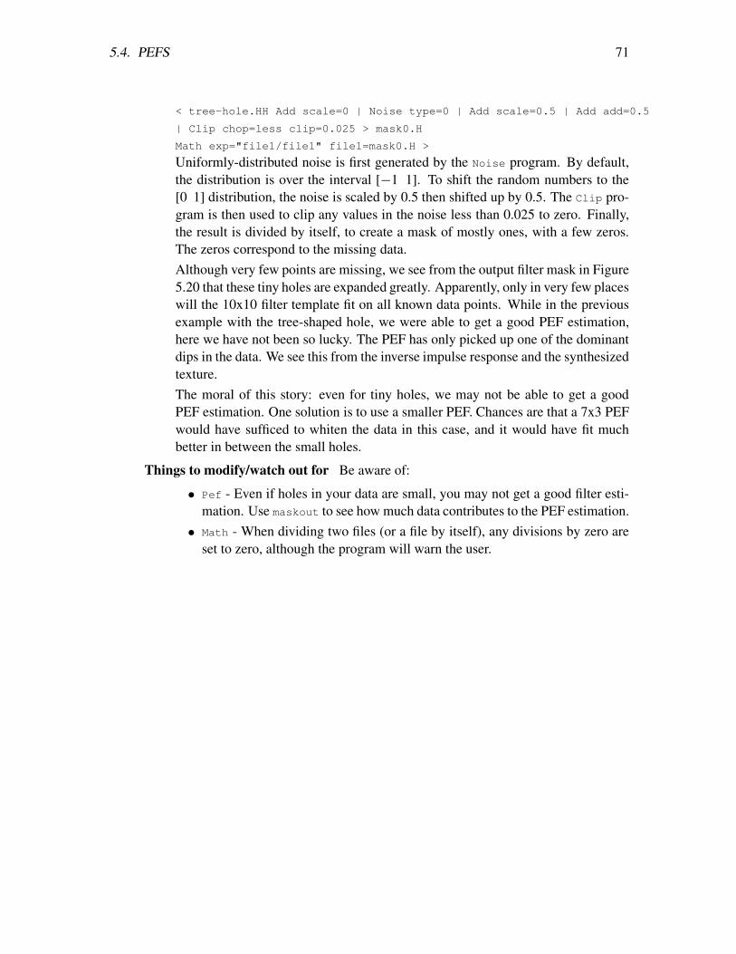
5.4. PEFS 71
< tree-hole.HH Add scale=0 | Noise type=0 | Add scale=0.5 | Add add=0.5
| Clip chop=less clip=0.025 > mask0.H
Math exp="file1/file1" file1=mask0.H >
Uniformly-distributed noise is first generated by the Noise program. By default,the distribution is over the interval [−1 1]. To shift the random numbers to the[0 1] distribution, the noise is scaled by 0.5 then shifted up by 0.5. The Clip pro-gram is then used to clip any values in the noise less than 0.025 to zero. Finally,the result is divided by itself, to create a mask of mostly ones, with a few zeros.The zeros correspond to the missing data.Although very few points are missing, we see from the output filter mask in Figure5.20 that these tiny holes are expanded greatly. Apparently, only in very few placeswill the 10x10 filter template fit on all known data points. While in the previousexample with the tree-shaped hole, we were able to get a good PEF estimation,here we have not been so lucky. The PEF has only picked up one of the dominantdips in the data. We see this from the inverse impulse response and the synthesizedtexture.The moral of this story: even for tiny holes, we may not be able to get a goodPEF estimation. One solution is to use a smaller PEF. Chances are that a 7x3 PEFwould have sufficed to whiten the data in this case, and it would have fit muchbetter in between the small holes.
Things to modify/watch out for Be aware of:
• Pef - Even if holes in your data are small, you may not get a good filter esti-mation. Use maskout to see how much data contributes to the PEF estimation.• Math - When dividing two files (or a file by itself), any divisions by zero are
set to zero, although the program will warn the user.
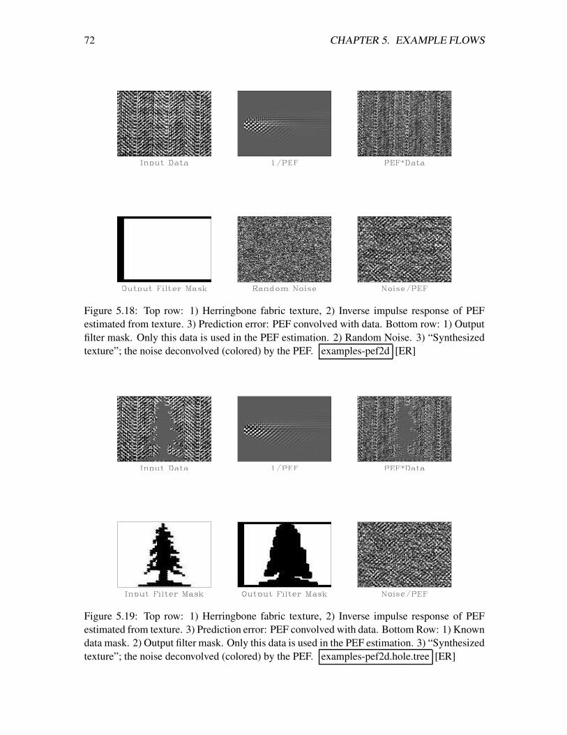
72 CHAPTER 5. EXAMPLE FLOWS
Figure 5.18: Top row: 1) Herringbone fabric texture, 2) Inverse impulse response of PEFestimated from texture. 3) Prediction error: PEF convolved with data. Bottom row: 1) Outputfilter mask. Only this data is used in the PEF estimation. 2) Random Noise. 3) “Synthesizedtexture”; the noise deconvolved (colored) by the PEF. examples-pef2d [ER]
Figure 5.19: Top row: 1) Herringbone fabric texture, 2) Inverse impulse response of PEFestimated from texture. 3) Prediction error: PEF convolved with data. Bottom Row: 1) Knowndata mask. 2) Output filter mask. Only this data is used in the PEF estimation. 3) “Synthesizedtexture”; the noise deconvolved (colored) by the PEF. examples-pef2d.hole.tree [ER]
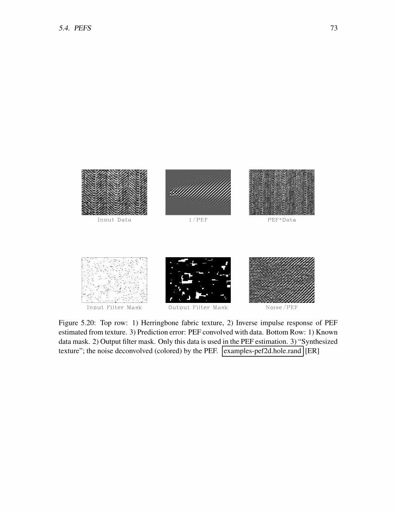
5.4. PEFS 73
Figure 5.20: Top row: 1) Herringbone fabric texture, 2) Inverse impulse response of PEFestimated from texture. 3) Prediction error: PEF convolved with data. Bottom Row: 1) Knowndata mask. 2) Output filter mask. Only this data is used in the PEF estimation. 3) “Synthesizedtexture”; the noise deconvolved (colored) by the PEF. examples-pef2d.hole.rand [ER]

74 CHAPTER 5. EXAMPLE FLOWS
Chapter 6
Tricky things
6.1 Piping in SEP3d
Piping is an incredibly useful feature to avoid creating numerous junk files in your directoryand on the scratch disks. The general rule for piping SEPlib programs (not SEP3D) is thatyou can’t seek on anything going through a pipe. For example, if you run < in.H First.x
|Second.x >out.H , First.x can seek its input and Second.x can seek its output but theconverse is not possible. The same rule applies to SEP3D. As long as you are doing sequentialaccessing of the headers, grid, and data, you can pipe from one SEP3D program to another. Forexample, you can pipe <in.H Headermath | Headermath >out.H, but not <in.H Headermath
| Sort3d >out.H because Sort3d does backward and forward seeks on its input and outputwhen reordering the traces.
6.2 Handling large files
One problem when handling 3-D data is the large size. Much of SEPlib used an int to specifythe location within a file. Unfortunately, the dynamic range of an int is limited to 2GB. Asa result, many of the SEPlib library had to be rewritten to handle the additional file size ina rather opaque manner1 that could still efficiently access files. In addition to dealing withthe 2GB limit in our own software, we had to overcome problems with Unix systems andstandards that did not account for more than 2GB file sizes. For example, only recently hasLinux begun to support file sizes over 2GB and portable tar’s are limited to 2GB files. Toget around these limitations Dave Nichols wrote some preliminary support for multiple-filedatasets. This support has been expanded upon to allow the user to create a dataset composedof multiple files, each not exceeding a user provided file size in Megabytes filesize.
The support for multiple file dataset provided two other benefits. First, the dreaded File
system full error is avoided. By specifying multiple directories for the datapath datap-
1There is no machine independent way to specify an integer with more dynamic range.
75
76 CHAPTER 6. TRICKY THINGS
ath=/scrka1/bob/;/scrka2/bob/ SEPlib will switch the directory it’s writing its binary datato when the file system is full or when a user-specified size limit (dirsize) is reached. Sec-ond, Cat3d can create a virtual SEPlib dataset by concatenating and updating grid and headerpointers, but leaving the large binary data files untouched.
The initial implementation of SEP3D did not allow piping between programs. As a result,many large, intermediate results were required. The new version of SEPlib allows piping byopening up additional sockets for the header and the grid. However piping is only allowedbetween SEP3D programs when certain conditions are met:
• init_3d() is called at the beginning of the program
• sep_3d_close() is called before the first writing of data
• no parameters (such as the number of traces) are changed after sep_3d_close
• data is written sequentially by the first program and read sequentially by the second
• the first and second programs read and write the same type of information (data, header,and/or grid)
6.3 Fancy plotting
6.3.1 Advanced plotting
Now we would like to introduce you to some tricks that might help you to demonstrate yourresults better. Often it is useful and spectacular to plot a Wiggle plot on top of a raster plot.That is a little tricky, but not too hard. First make our windowed input data again (if we don’tstill have it):
Window < Txx.HH min1=.4 max1=.8 max2=1. > Txx_Windowed.H
Now run Ta2vplot once to make the “background” raster plot:
Byte < Txx_Windowed.H pclip=100 | \
Ta2vplot par=plotpar.p min1=.4 max1=.8 max2=1. min2=.05 \
out=file1.v head=/dev/null
The out=file1.v tells Ta2vplot to write the output to “file1.v”; the head=/dev/null throwsthe output history file away to the UNIX garbage-can device “/dev/null”.) Finally we runWiggle twice, once with thick “invisible” traces and once with half as thick standard yellowones:
6.3. FANCY PLOTTING 77
Wiggle < Txx_Windowed.H par=plotpar.p min1=.4 max1=.8 max2=1. min2=.05 \
poly=no out=file2.v head=/dev/null plotcol=0 plotfat=10
Wiggle < Txx_Windowed.H par=plotpar.p min1=.4 max1=.8 max2=1. min2=.05 \
poly=no out=file3.v head=/dev/null plotfat=5
Note how we had to specify all four limits to be sure that the plots produced by the verydifferent plotting programs Ta2vplot and Wiggle would be compatible. (For some other plotprograms even this isn’t enough; we also have to turn off the “padding” between plot andaxes.) Now for the “advanced graphics”: to combine the three plots, we use a special penfilter called “vppen”, which reads in and writes out the vplot graphical files used by SEPlibprograms.
vppen file1.v file2.v file3.v erase=once vpstyle=no | tube
vppen is not itself a SEPlib program, hence the lower-case initial letter and why we had to useout= above. (There is a SEPlib version called Vppen that we could have used, but history filesbecome less useful at this point.) Note that we didn’t really need to use vppen above; we couldhave just done
tube file1.v file2.v file3.v erase=once
directly. It is useful to do such manipulations with vppen because it lets us save the compositeplot as a single vplot file, in effect “flattening” the composite into a single plot. There is nomagic involved here; vppen is a vplot pen filter just like tube, and shares almost all the samecode. The only difference is that while tube draws plots on screens, vppen writes out “vplotgraphical language”. Suppose you plot something on your screen using tube with complexoptions and multiple input files, and want to somehow save your graphical masterpiece insuch a way that you can reproduce it again later without so much trouble with options andfiles. Simple: just replace tube with vppen and redirect the output. You have now saved yourmasterpiece as a single vplot file. If you are looking at our example plot on your screen rightnow you might be wondering why we went to the trouble of creating the “invisible wiggles”file file2.v. We hope that after you examine the hardcopy version in Figure 6.1 the reasonshould become evident! Examining Figure 6.1 you may also notice there are two titles. Whilevarious plot programs like Wiggle and Ta2vplot are consistent in their options for things likewhere to put the title, which way to put axes, etc, for historical reasons they are not consistentin their defaults. So if you want to get plots from different programs to exactly overlay ingeneral you have to specify everything. Since we did not specify whether to put the title aboveor below the plot, we got the (different) default for each. You shouldn’t have trouble gettingaround such annoyances. (Usually you just turn off the axes and labels for all the parts butone.)
6.3.2 Plot matrices
Perhaps the previous example seemed a little technical for you. How about this one then?Often you want to compare two plots side by side (or squeeze more figures into your expanded
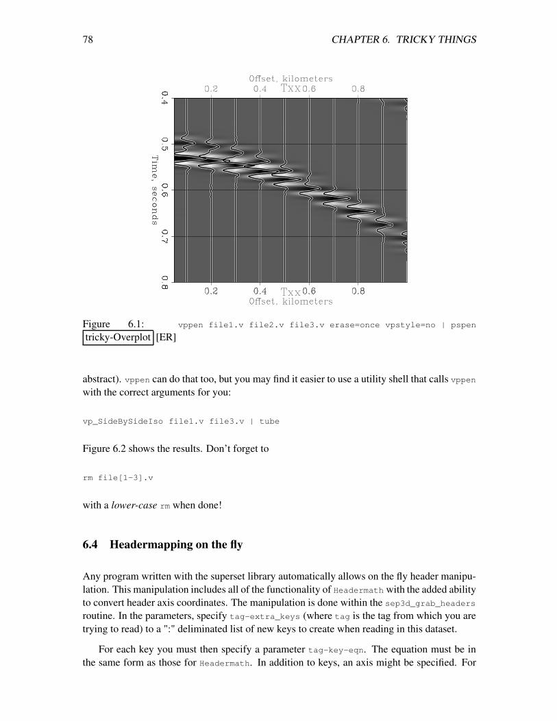
78 CHAPTER 6. TRICKY THINGS
Figure 6.1: vppen file1.v file2.v file3.v erase=once vpstyle=no | pspen
tricky-Overplot [ER]
abstract). vppen can do that too, but you may find it easier to use a utility shell that calls vppenwith the correct arguments for you:
vp_SideBySideIso file1.v file3.v | tube
Figure 6.2 shows the results. Don’t forget to
rm file[1-3].v
with a lower-case rm when done!
6.4 Headermapping on the fly
Any program written with the superset library automatically allows on the fly header manipu-lation. This manipulation includes all of the functionality of Headermath with the added abilityto convert header axis coordinates. The manipulation is done within the sep3d_grab_headers
routine. In the parameters, specify tag-extra_keys (where tag is the tag from which you aretrying to read) to a ":" deliminated list of new keys to create when reading in this dataset.
For each key you must then specify a parameter tag-key-eqn. The equation must be inthe same form as those for Headermath. In addition to keys, an axis might be specified. For
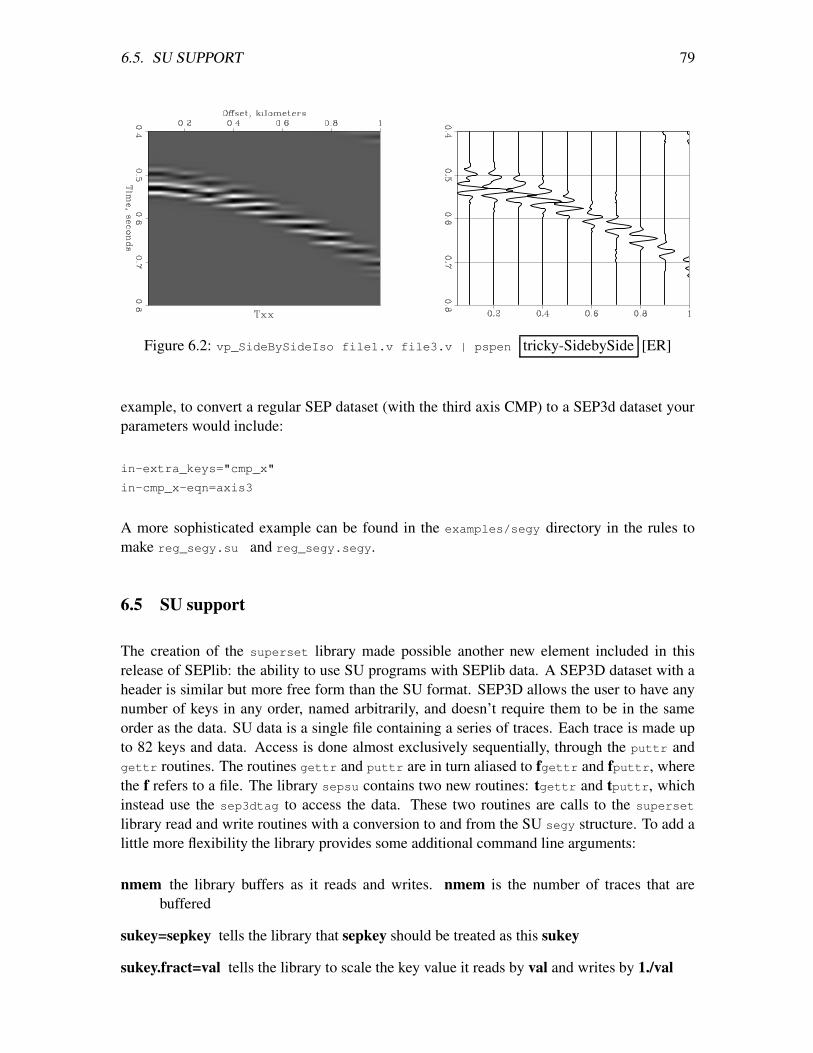
6.5. SU SUPPORT 79
Figure 6.2: vp_SideBySideIso file1.v file3.v | pspen tricky-SidebySide [ER]
example, to convert a regular SEP dataset (with the third axis CMP) to a SEP3d dataset yourparameters would include:
in-extra_keys="cmp_x"
in-cmp_x-eqn=axis3
A more sophisticated example can be found in the examples/segy directory in the rules tomake reg_segy.su and reg_segy.segy.
6.5 SU support
The creation of the superset library made possible another new element included in thisrelease of SEPlib: the ability to use SU programs with SEPlib data. A SEP3D dataset with aheader is similar but more free form than the SU format. SEP3D allows the user to have anynumber of keys in any order, named arbitrarily, and doesn’t require them to be in the sameorder as the data. SU data is a single file containing a series of traces. Each trace is made upto 82 keys and data. Access is done almost exclusively sequentially, through the puttr andgettr routines. The routines gettr and puttr are in turn aliased to fgettr and fputtr, wherethe f refers to a file. The library sepsu contains two new routines: tgettr and tputtr, whichinstead use the sep3dtag to access the data. These two routines are calls to the superset
library read and write routines with a conversion to and from the SU segy structure. To add alittle more flexibility the library provides some additional command line arguments:
nmem the library buffers as it reads and writes. nmem is the number of traces that arebuffered
sukey=sepkey tells the library that sepkey should be treated as this sukey
sukey.fract=val tells the library to scale the key value it reads by val and writes by 1./val
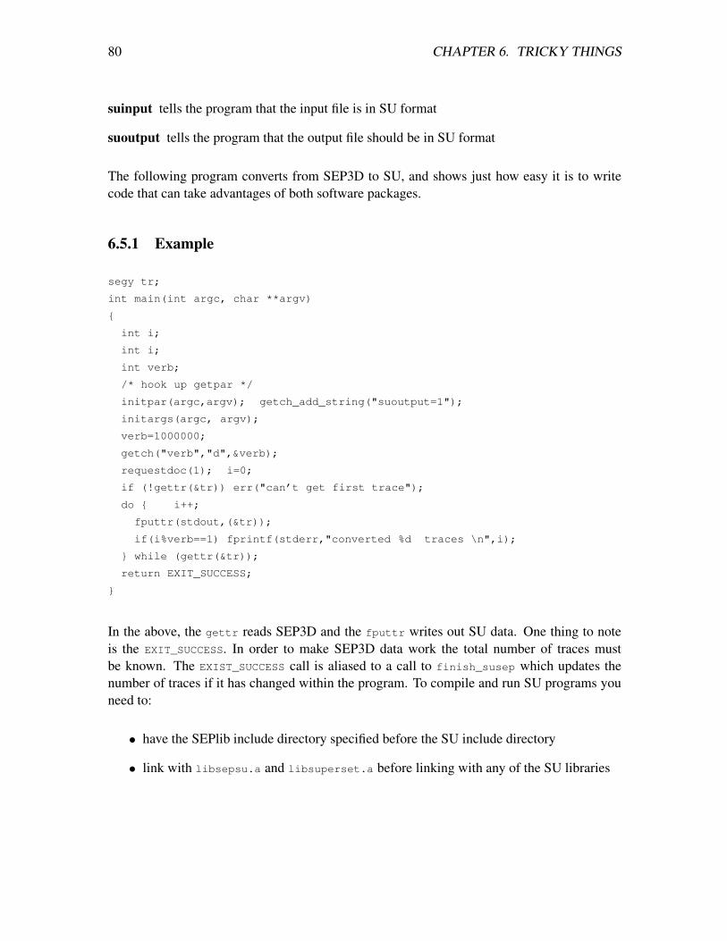
80 CHAPTER 6. TRICKY THINGS
suinput tells the program that the input file is in SU format
suoutput tells the program that the output file should be in SU format
The following program converts from SEP3D to SU, and shows just how easy it is to writecode that can take advantages of both software packages.
6.5.1 Example
segy tr;
int main(int argc, char **argv)
{
int i;
int i;
int verb;
/* hook up getpar */
initpar(argc,argv); getch_add_string("suoutput=1");
initargs(argc, argv);
verb=1000000;
getch("verb","d",&verb);
requestdoc(1); i=0;
if (!gettr(&tr)) err("can’t get first trace");
do { i++;
fputtr(stdout,(&tr));
if(i%verb==1) fprintf(stderr,"converted %d traces \n",i);
} while (gettr(&tr));
return EXIT_SUCCESS;
}
In the above, the gettr reads SEP3D and the fputtr writes out SU data. One thing to noteis the EXIT_SUCCESS. In order to make SEP3D data work the total number of traces mustbe known. The EXIST_SUCCESS call is aliased to a call to finish_susep which updates thenumber of traces if it has changed within the program. To compile and run SU programs youneed to:
• have the SEPlib include directory specified before the SU include directory
• link with libsepsu.a and libsuperset.a before linking with any of the SU libraries
Chapter 7
Makerules
Make is a smart scripting language for generating commands. The syntax for make can bequite simple or quite complex. Schwab (1996) provides information on SEP’s philosophyand how we use make for our reproducible documents. For a complete description of makefeatures type xinfo (or look in /usr/local/src/gnu/make-* the files of the form make.info-*contain the source for xinfo). Another good source for examples are old SEP reports.
7.1 Compile Rules
SEP has a fairly sophisticated set of make rules to make compiling programs easier. To useSEP’s make rules you need to put at the top of your makefile:
include ${SEPINC}/SEP.top
and at the bottom of your Makefile:
include ${SEPINC}/SEP.bottom
All of SEP’s compiling rules are based on using a standard suffix convention so let’s start bylisting the acceptable suffixes:
• .c : C code
• .C : C++ code
• .java : java code
• Fortran77
– .f : strict fortran77 code
81
82 CHAPTER 7. MAKERULES
– .r : ratfor code
– .rs : ratfor with SAW conventions
– .rst : ratfor with SAW conventions and temporary arrays
– .rt : ratfor code with temporary arrays
• Fortran90
– .f90 : strict fortran90 code
– .r90 : ratfor90 code (similar to ratfor)
– .rs90 : ratfor90 code + saw conventions
As your program becomes more complex (more files, libraries, compiling options, etc.) yourMakefile complexity increases similarly.
• In the simplest case, when you write a program that is contained in a single C, Fortran77,Fortran90, or C++ file (for example program.c) you just have to type gmake program.x
to compile the program and to link it with SEP and system libraries.
• If you want to link additional object files to create the executable add the rule:
program.x: subs.o
where subs.suffix (the list above) is another source file in which you wish the exe-cutable to be linked with.
• If this level of sophistication is not sufficient there exist a number of predefined variablesthat you can add to your Makefile that perform special functions. Below is a list of thevariables, what they do, and where they must be placed in the Makefile. All of thevariables need to be assigned in the following manner:
VAR = mydefinition
– Debugging/Optimization
– DEBUG [before SEP.top], set it equal to anything and the program will compile indebug mode. If you plan to use a debugger on your code YOU MUST set this flag.
�OLEVEL [before SEP.top] sets the optimization to manual control. It defaultsto a fairly intelligent value, so you should normally not set this.
�NO_FIX [before SEP.top], keeps .f90 files (created from .r90 and .rs90 files).You need this if you’re using a debugger.
– Adding libraries : when you write more complex programs you will often createyour own library. To link with this library using the standard make rules you needto define the following variables:
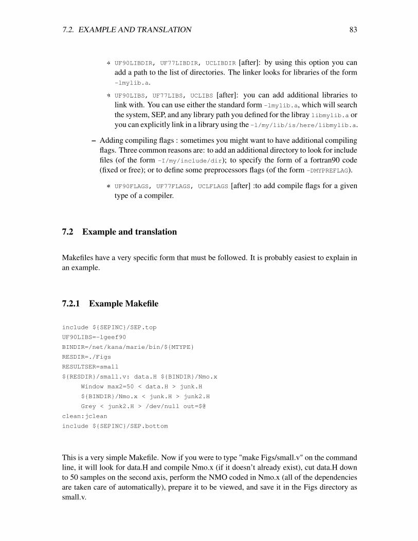
7.2. EXAMPLE AND TRANSLATION 83
�UF90LIBDIR, UF77LIBDIR, UCLIBDIR [after]: by using this option you canadd a path to the list of directories. The linker looks for libraries of the form-lmylib.a.
�UF90LIBS, UF77LIBS, UCLIBS [after]: you can add additional libraries tolink with. You can use either the standard form -lmylib.a, which will searchthe system, SEP, and any library path you defined for the libray libmylib.a oryou can explicitly link in a library using the -l/my/lib/is/here/libmylib.a.
– Adding compiling flags : sometimes you might want to have additional compilingflags. Three common reasons are: to add an additional directory to look for includefiles (of the form -I/my/include/dir); to specify the form of a fortran90 code(fixed or free); or to define some preprocessors flags (of the form -DMYPREFLAG).
�UF90FLAGS, UF77FLAGS, UCLFLAGS [after] :to add compile flags for a giventype of a compiler.
7.2 Example and translation
Makefiles have a very specific form that must be followed. It is probably easiest to explain inan example.
7.2.1 Example Makefile
include ${SEPINC}/SEP.top
UF90LIBS=-lgeef90
BINDIR=/net/kana/marie/bin/${MTYPE}
RESDIR=./Figs
RESULTSER=small
${RESDIR}/small.v: data.H ${BINDIR}/Nmo.x
Window max2=50 < data.H > junk.H
${BINDIR}/Nmo.x < junk.H > junk2.H
Grey < junk2.H > /dev/null out=$@
clean:jclean
include ${SEPINC}/SEP.bottom
This is a very simple Makefile. Now if you were to type "make Figs/small.v" on the commandline, it will look for data.H and compile Nmo.x (if it doesn’t already exist), cut data.H downto 50 samples on the second axis, perform the NMO coded in Nmo.x (all of the dependenciesare taken care of automatically), prepare it to be viewed, and save it in the Figs directory assmall.v.
84 CHAPTER 7. MAKERULES
7.2.2 Translation
This is a line-by-line translation of the example Makefile.
include ${SEPINC}/SEP.top and include ${SEPINC}/SEP.bottom : these must be includedto use SEP’s make rules.
UF90LIBS=-lgeef90 : this adds a Fortran90 library to link to. You can also use UF90LIBDIRto provide a path to extra Fortran90 libraries. You may also use UF77LIBS/DIR and UCLIBS/DIR.See the Libraries chapter for descriptions of the contents of each library.
BINDIR=/net/kana/marie/bin/${MTYPE} : this tells the make rules where to find the exe-cutables you want to use. In this case, I am using files on marie’s personal device in her bindirectory and the MTYPE lets the make rules decide which subdirectory it needs (MachineTYPE).
RESDIR=./Figs : this tells the make rules where to put your results, in this case the "Figs"directory.
RESULTSER=small : the only Easily Reproducible RESULT you get from this Makefile is"small". You could also have RESULTSNR (Non-Reproducible) and/or RESULTSCR (Con-ditionally Reproducible).
${RESDIR}/small.v: data.H ${BINDIR}/Nmo.x : here you state what your target is (we wantto make Figs/small.v) and what it depends on (we must have data.H and /net/kana/marie/bin/SGI64/Nmo.x).
Window max2=50 < data.H > junk.H : this pulls a section of the data out and puts it injunk.H. IMPORTANT NOTE: after the line which contains the target and dependencies, all ofthe lines for this target MUST begin with a TAB. You can’t use spaces, you must use TAB.Remember when you copy and paste the tab may become spaces - you must replace them witha TAB.
${BINDIR}/Nmo.x < junk.H > junk2.H : now we feed junk.H into the NMO program andget the result junk2.H.
Grey < junk2.H > /dev/null out=$@ : finally we can prepare the file for viewing. Ratherthan having to restate the target’s name, here you can simply call it $@. Note that when using"Grey" to make a .v file you must specify the results as "out=" and output to /dev/null.
clean:jclean : this is the clean rule. When you type "make clean" on the command line thiswill remove all intermediate files to clean up your directory.
REFERENCES
Schwab, M., Karrenbach, M., and Claerbout, J., 1996, Making scientific computations repro-ducible: submitted for publication in Computer in Physics, ??, ??
Chapter 8
Libraries
SEPlib and SEP3D are designed to carry out fairly simple, commonly used operations ondatasets. Through the years many additional subroutines/functions have been written to per-form more complicated processing on SEPlib and SEP3D datasets, or to be used by otherprograms. Many of these have been organized in various libraries. This chapter gives briefdescriptions of many of the subroutines/functions available in our libraries. Better descriptionscan be obtained through self-documentation (not available for everything listed here) or on-line at http://sepwww.stanford.edu/software/seplib/html_docs/index.html. Knowingwhich subroutines/functions are in which library becomes important when you write complexprograms and use makefiles, as described in the Makerules chapter.
8.1 Summary of libraries
sep This is the SEPlib base library.
sep3d This is the SEP3D base library.
sep2df90 This is the library containing the Fortran90 interface for handling sep2d datasets.
supersetf90 This is the library containing the Fortran90 interface for handling SEP3D datasets.
sepaux This is the library that catches all of the useful functions that don’t fit anywhere else.
sepauxf90 This is the library that catches all of the useful Fortran90 functions that don’t fitanywhere else.
geef90 This is the Fortran90 GEE (Geophysical Estimation by Example) operator library.
sepfilter This is the library containing functions that deal with filtering.
sepfilterf90 This is the Fortran90 library containing functions that deal with filtering.
sepfft This is the library containing functions that do FFTs.
85
86 CHAPTER 8. LIBRARIES
septravel This is the library containing functions that calculate traveltimes.
sepvelanf This is the library containing Fortran77 functions that deal with velocity.
sepvelanf90 This is the library containing Fortran90 functions that deal with velocity.
sepmath This library contains math functions, especially complex C functions.
sepmathf90 This library contains Fortran90 math functions.
sepsu This library contains functions that allow SEPlib and SU to interface.
sepoclibf90 This is the Fortran90 out-of-core inversion library.
sepweif90 Library for performing wave equation migration.
sepmpi/sepmpif/sepmpif90 Library for doing mpi with SEPlib files.
8.2 Library: sep
This is the SEPlib base library.
auxclose Close a SEPlib history file
auxpar Get a parameter from auxiliary file
sepwarn Print a string and return a specified value
evaluate_expression Evaluate a mathematical expression
puthead Put a formatted string to SEPlib history file
auxputhead Put a formatted string to SEPlib auxiliary history file
make_unpipe Unpipe a SEPlib file (therefore back seekable)
getch Grab a parameter from command line
getch_add_string Add parameters to the command line
fetch Grab a parameter from the command line or history file
hetch Grab a parameter from input history file
putch Put an argument in output history file
doc Program self documentation
sreed Read in an array from a SEPlib file
8.3. LIBRARY: SEP3D 87
sseek Seek to a position in a SEPlib dataset
sseek_block Seek to a position in a SEPlib dataset by blocks
seperr Print line and exit with a failure code
initpar Initiate SEPlib I/O parameter handling
datapath The datapath to put seplib binaries
copy_history Copy the contents of one history file to another.
srite Write an array to SEPlib tag
ssize Obtain the size of a SEPlib file
ssize_block Obtain the number of blocks in a SEPlib file
auxputch Put a parameter into auxiliary file
sreed_window Read a window of a SEPlib dataset
srite_window Write a SEPlib window
fullnm Expand a filename to a fully qualified name with all path prefixes
alloc Allocate a C array with error checking
slice Write an array to the screen (through Grey etc)
h2c Convert from helical to cartersian coordinates
c2h Convert from cartesian to helical coordinates
hclose Close the SEPlib output history file
8.3 Library: sep3d
This is the SEP3D base library.
sep_put_number_keys Put the number of keys
sep_get_val_headers Get the header values
sep_put_val_by_index Puts the header value into the header values file by index
sep_reorder_data Reorder the traces of a SEPlib dataset
sep_get_number_data_axes Get the number of data axes
88 CHAPTER 8. LIBRARIES
sep_get_number_header_axes Get the number of header axes
sep_get_number_grid_axes Get the number of grid axes
copy_data_pointer Copy the data pointer from one file to another
sep_set_no_headers Set no headers to an output tag
sep_set_no_grid Set that the output tag does not have a grid
sep_copy_gff Copy the grid format file from one SEP3D file to another
sep_copy_hff Copy the header format file from one SEP3D file to another
sep_extract_val_by_index Extract a header value by its index
sep_get_key_name Get the key name associated with a key index
sep_get_val_by_name Get the header value by name
sep_3d_close Close SEP3D format files
sep_get_number_keys Get the number of keys
sep_get_key_fmt Get the format of a key
sep_put_val_headers Write a header block
init_3d Initialize SEP3D I/O
sep_get_key_index Get the index of a key
sep_copy_header_keys Copy keys from one SEP3D file to another
sep_put_key Write the key info to a tag
sep_put_grid_window Write a window of the grid
sep_get_grid_window Read a window of the grid
sep_copy_grid Copy a grid from one tag to another
sep_get_data_axis_par Grab data’s n,o,d and label
sep_get_header_axis_par Grab headers’s n,o,d and label
sep_get_grid_axis_par Grab grid’s n,o,d and label
sep_get_key_type Get the key type associated with an index
sep_put_header_axis_par Put n,o,d, label of the headers to output tag
sep_put_data_axis_par Put n,o,d, label of the data to output tag
sep_put_grid_axis_par Put n,o,d, label of the grid to output tag
8.4. LIBRARY: SEP2DF90 89
8.4 Library: sep2df90
This is the library containing the Fortran90 interface for handling sep2d datasets.
from_history Grab parameters from the history file
from_aux Grab parameters from an auxiliary file
from_param Grab parameters from the command line or parameter file
from_either Grab parameters from the command line, parameter file or history file
to_history Store parameters in the output history file
sep_read Read a SEPlib dataset
sep_write Write a SEPlib dataset
sep_init Initialize a SEPlib dataset
sep_close Close a SEPlib format file
sep_dimension Returns the number of dimensions in dataset
8.5 Library: supersetf90
This is the library containing the Fortran90 interface for handling SEP3D datasets.
sep3df SEP3D Fortran90 structure (superset)
init_sep3d Initialize a SEP3d type
sep3d_grab_key_vals Grab header values from a C structure
sep3d_set_key_vals Set header values in a C structure
sep3d_read_data Read in data
sep3d_write_data Write out data
sep3d_grab_sep3d Synchronize f90 structure with C structure
sep3d_set_sep3d Synchronize C structure with f90 structure
valid_structure Check if SEP3d structure is valid
sep3d_grab_headers Grab the headers
sep3d_write_description Write out the format file info
90 CHAPTER 8. LIBRARIES
sep3d_add_drn Add data record number
sep3d_key_index Try to find a key in a structure
sep3d_axis_index Try to find a axis in a structure
sep3d_set_number_headers Set the number of headers to store
sep3d_store_grid_values Store a grid
8.6 Library: sepaux
This is the library that catches all of the useful functions that don’t fit anywhere else.
pad_it Pad an array
cent nth percentile of an array
pqueue Heap priority queue
sgainpar Gain seismic data
8.7 Library: sepauxf90
This is the library that catches all of the useful Fortran90 functions that don’t fit anywhereelse.
interpolate_mod Linear interpolation
quick_sort Quick sort
8.8 Library: geef90
This is the Fortran90 GEE (Geophysical Estimation by Example) operator library. Expandeddescriptions can be found in GEE, which is on-line.
mspef Find a multi-scale prediction error filter
lopef Estimate a pef in patches
pef Find a prediction error filter
npef Find a non-stationary prediction error filter
8.8. LIBRARY: GEEF90 91
createhelix Create a helix filter
helix Module containing allocate and deallocate of a helix filter
createnhelix Create a non-stationary helix filter
nhelix Module containing allocate and deallocate of a nhelix filter
createmshelix Create a multi-scale helix filter
compress Compress a helix filter
helderiv Helix derivative filter
nhelicon Non-stationary convolution
helicon Convolution using helix filters
heliarr Two helix convolutions
regrid Convert a helix filter from one data space to another
helixcartmod Convert to and from cartesian/helix space
conv Convolve helix filters
hconest Convolution using helix filters, adjoint is filter
nhconest Non-stationary convolution using helix filters, adjoint is filter
mshconest Convolution using multi-scale helix filters, adjoint is filter
wilson Wilson’s factorization
cross_wilson Wilson factorization of cross-correlation
mshelicon Convolution using multi-scale helix filters
pefest Find a prediction error filter, avoiding bursty noise
mis2 Fill in missing data
nmis2 Fill in missing data using a non-stationary filter
bound Find the boundaries of a filter on given map
nbound Find the boundaries of a multi-scale filter on given map
conjgrad One step of the conjugate gradient solver
cdstep One step of the conjugate direction solver
cgstep One step of the conjugate gradient solver
92 CHAPTER 8. LIBRARIES
cgmeth Conjugate gradient method
gauss Solve a system by gaussian elimination
lsqr Solve a system of using lsqr method
solver Solve a system of equations
solver_reg Iteratively solve a regularized system of equations
solver_prec Iteratively solve a preconditioned system of equations
nonlin_solver Generic non-linear solver program
irls Weighting functions for least-squares
lint1 1-D linear interpolation
lint2 2-D linear interpolation
dottest Perform a dot product test on an operator
ddot Calculate double precision dot product
autocorr Compute a filter’s auto-correlation
binpull1 Nearest neighbor interpolation
binpull2 Nearest neighbor interpolation, 2D
invint Inverse linear interpolation
lapfac Factor a 2-D Laplacian
signoi Signal and noise separation
partan Partan step
box Filter to hypercube
cartesian Convert to and from cartesian coordinates
chain Create a chain of 2,3, or 4 operators
array Create an array operator
polydiv Polynomial division
npolydiv Non-stationary polynomial division
steering 2-D steering filters
weight Simple weighting operator
8.9. LIBRARY: SEPFILTER 93
misinput Find a mask of missing filter inputs
adj_mod Simple adjnull function
causint Causal integration
cdoubint Double causal integration
matmult Matrix multiplication
triangle Triangle smoothing
triangle1 Triangle smoothing
triangle2 Triangle smoothing
quantile Find quantile of the data
igrad1 1D gradient operator
igrad2 2D gradient operator
refine2 Refine mesh
msmis Fill in missing data using a multi-scale filter
steepdip Find a steep dip decon filter
patch Extract and put back patches
8.9 Library: sepfilter
This is the library containing functions that deal with filtering.
energy Calculate energy in running windows along fast data axis
8.10 Library: sepfilterf90
This is the Fortran90 library containing functions that deal with filtering.
burg Burg deconvolution
burg2 Burg 2D convolution
butter Find a Butterworth filter
halfdifa Half causal derivative
boxconv Smooth by applying a box filter
94 CHAPTER 8. LIBRARIES
8.11 Library: sepfft
This is the library containing functions that do FFTs.
refft Real FFT along one trace
rvfft Real vector FFT
cefft Complex FFT along one trace
cvfft Complex vector FFT
8.12 Library: septravel
This is the library containing functions that calculate traveltimes.
hwt_trace_rays Ray tracing using Huygens wavefront tracing
hwt_travel_cube Get travel times by Huygens wavefront tracing and then interpolate
fastmarch Get travel times using eikonal solver
8.13 Library: sepvelanf
This is the library containing Fortran77 functions that deal with velocity.
veltran Velocity transform with anti-aliasing and√
iω
rms2int Convert to and from rms/interval velocity
velsimp Simple velocity transform
8.14 Library: sepvelanf90
This is the library containing Fortran90 functions that deal with velocity.
nmo_mod Perform NMO
velan_subs_mod Do semblance analysis
8.15. LIBRARY: SEPMATH 95
8.15 Library: sepmath
This library contains math functions, especially complex C functions.
cmplx Create a complex number
cspow Raise a complex number to real power
cadd Add complex numbers
csqrt Take the square root of a complex number
csub Subtract complex numbers
cdiv Divide complex numbers
csmult Multiply a complex number by a scalar
cmult Multiply complex numbers
cexp Returns exp(complex number)
ciexp Returns exp(imaginary number)
cinv Inverse of a complex number
clog Complex log
cneg Negative of a complex number
conj Complex conjugate
sqroot Square root
8.16 Library: sepmathf90
This library contains Fortran90 math functions.
hermtoep Solve a hermitian toeplitz system
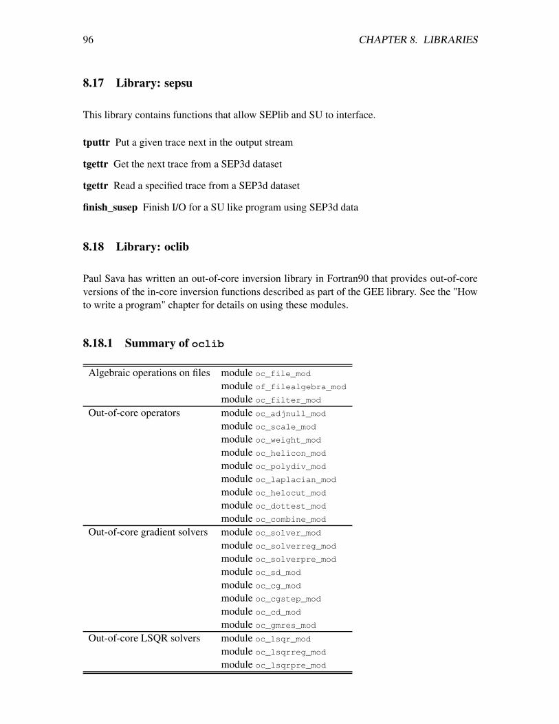
96 CHAPTER 8. LIBRARIES
8.17 Library: sepsu
This library contains functions that allow SEPlib and SU to interface.
tputtr Put a given trace next in the output stream
tgettr Get the next trace from a SEP3d dataset
tgettr Read a specified trace from a SEP3d dataset
finish_susep Finish I/O for a SU like program using SEP3d data
8.18 Library: oclib
Paul Sava has written an out-of-core inversion library in Fortran90 that provides out-of-coreversions of the in-core inversion functions described as part of the GEE library. See the "Howto write a program" chapter for details on using these modules.
8.18.1 Summary of oclib
Algebraic operations on files module oc_file_mod
module of_filealgebra_mod
module oc_filter_mod
Out-of-core operators module oc_adjnull_mod
module oc_scale_mod
module oc_weight_mod
module oc_helicon_mod
module oc_polydiv_mod
module oc_laplacian_mod
module oc_helocut_mod
module oc_dottest_mod
module oc_combine_mod
Out-of-core gradient solvers module oc_solver_mod
module oc_solverreg_mod
module oc_solverpre_mod
module oc_sd_mod
module oc_cg_mod
module oc_cgstep_mod
module oc_cd_mod
module oc_gmres_mod
Out-of-core LSQR solvers module oc_lsqr_mod
module oc_lsqrreg_mod
module oc_lsqrpre_mod
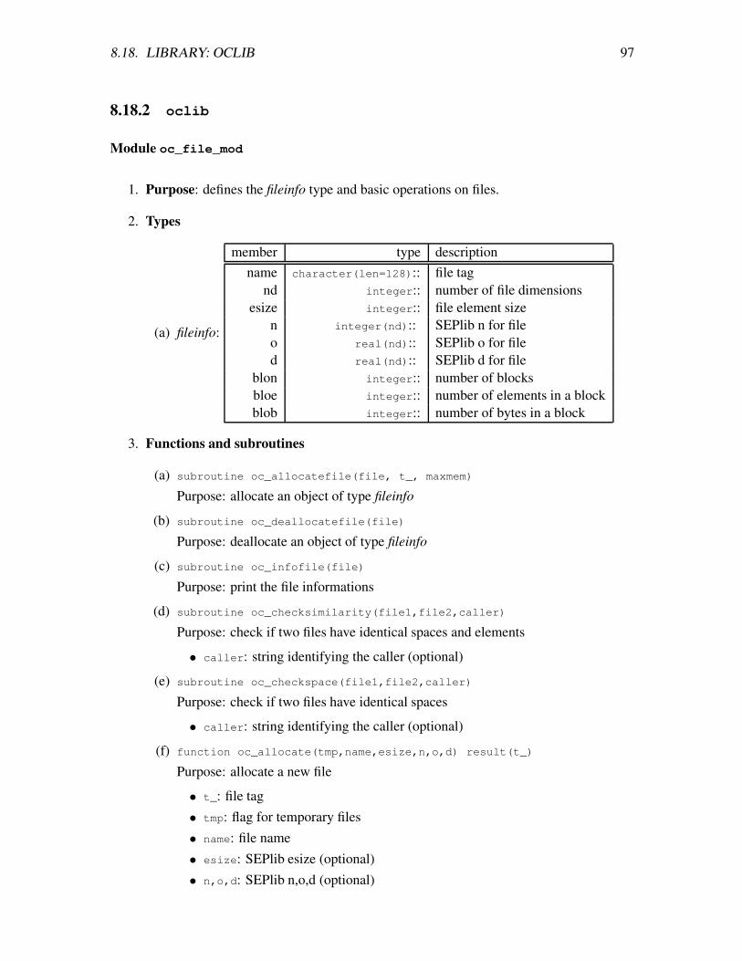
8.18. LIBRARY: OCLIB 97
8.18.2 oclib
Module oc_file_mod
1. Purpose: defines the fileinfo type and basic operations on files.
2. Types
(a) fileinfo:
member type descriptionname character(len=128):: file tag
nd integer:: number of file dimensionsesize integer:: file element size
n integer(nd):: SEPlib n for fileo real(nd):: SEPlib o for filed real(nd):: SEPlib d for file
blon integer:: number of blocksbloe integer:: number of elements in a blockblob integer:: number of bytes in a block
3. Functions and subroutines
(a) subroutine oc_allocatefile(file, t_, maxmem)
Purpose: allocate an object of type fileinfo
(b) subroutine oc_deallocatefile(file)
Purpose: deallocate an object of type fileinfo
(c) subroutine oc_infofile(file)
Purpose: print the file informations
(d) subroutine oc_checksimilarity(file1,file2,caller)
Purpose: check if two files have identical spaces and elements
• caller: string identifying the caller (optional)
(e) subroutine oc_checkspace(file1,file2,caller)
Purpose: check if two files have identical spaces
• caller: string identifying the caller (optional)
(f) function oc_allocate(tmp,name,esize,n,o,d) result(t_)
Purpose: allocate a new file
• t_: file tag• tmp: flag for temporary files• name: file name• esize: SEPlib esize (optional)• n,o,d: SEPlib n,o,d (optional)
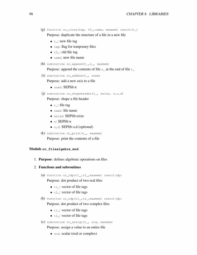
98 CHAPTER 8. LIBRARIES
(g) function oc_clone(tmp, t0_,name, maxmem) result(t_)
Purpose: duplicate the structure of a file in a new file
• t_: new file tag• tmp: flag for temporary files• t0_: old file tag• name: new file name
(h) subroutine oc_append(t_,s_, maxmem)
Purpose: append the contents of file s_ at the end of file t_
(i) subroutine oc_adddim(t_, nnew)
Purpose: add a new axis to a file
• nnew: SEPlib n
(j) subroutine oc_shapeheader(t_, esize, n,o,d)
Purpose: shape a file header
• t_: file tag• name: file name• esize: SEPlib esize• n: SEPlib n• o,d: SEPlib o,d (optional)
(k) subroutine oc_print(t_, maxmem)
Purpose: print the contents of a file
Module oc_filealgebra_mod
1. Purpose: defines algebraic operations on files
2. Functions and subroutines
(a) function oc_rdp(t1_,t2_,maxmem) result(dp)
Purpose: dot product of two real files
• t1_: vector of file tags• t2_: vector of file tags
(b) function oc_cdp(t1_,t2_,maxmem) result(dp)
Purpose: dot product of two complex files
• t1_: vector of file tags• t2_: vector of file tags
(c) subroutine oc_assign(t_, sca, maxmem)
Purpose: assign a value to an entire file
• sca: scalar (real or complex)
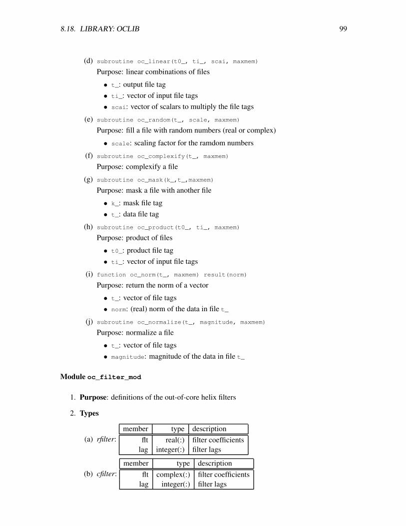
8.18. LIBRARY: OCLIB 99
(d) subroutine oc_linear(t0_, ti_, scai, maxmem)
Purpose: linear combinations of files
• t_: output file tag• ti_: vector of input file tags• scai: vector of scalars to multiply the file tags
(e) subroutine oc_random(t_, scale, maxmem)
Purpose: fill a file with random numbers (real or complex)
• scale: scaling factor for the ramdom numbers
(f) subroutine oc_complexify(t_, maxmem)
Purpose: complexify a file
(g) subroutine oc_mask(k_,t_,maxmem)
Purpose: mask a file with another file
• k_: mask file tag• t_: data file tag
(h) subroutine oc_product(t0_, ti_, maxmem)
Purpose: product of files
• t0_: product file tag• ti_: vector of input file tags
(i) function oc_norm(t_, maxmem) result(norm)
Purpose: return the norm of a vector
• t_: vector of file tags• norm: (real) norm of the data in file t_
(j) subroutine oc_normalize(t_, magnitude, maxmem)
Purpose: normalize a file
• t_: vector of file tags• magnitude: magnitude of the data in file t_
Module oc_filter_mod
1. Purpose: definitions of the out-of-core helix filters
2. Types
(a) rfilter:member type description
flt real(:) filter coefficientslag integer(:) filter lags
(b) cfilter:member type description
flt complex(:) filter coefficientslag integer(:) filter lags

100 CHAPTER 8. LIBRARIES
3. Functions and subroutines
(a) subroutine allocatehelix(aa, nh)
Purpose: allocate space for the filter coefficients
• aa: helix filter (real or complex)• nh: number of coefficients
(b) subroutine deallocatehelix(aa)
Purpose: deallocate filter space
• aa: helix filter (real or complex)
(c) subroutine buildfilter(ff,x_,fbox,nf,maxmem)
Purpose: build a helix filter
• ff: output filter (real or complex)• x_: file tag for the filtering space• fbox: multidimensional array with the filter coefficients• nf: number of coefficients
(d) subroutine printfilter(ff,nf)
Purpose: print the filter coefficients
• ff: filter (real or complex)• nf: number of coefficients
Module oc_adjnull_mod
1. Purpose: nullify the output of an operator
2. Functions and subroutines
(a) subroutine oc_adjnull(adj,add, x_,yy_)
Purpose: nullify operator output
Module oc_scale_mod
1. Purpose: scaling operator
2. Functions and subroutines
(a) subroutine oc_scale_init(eps,maxmem)
Purpose: initialize the scaling operator
• eps: scaling parameter (real or complex)
(b) function oc_scale(adj,add, x_,yy_,op1 ...op9) result(stat)
Purpose: scaling operator
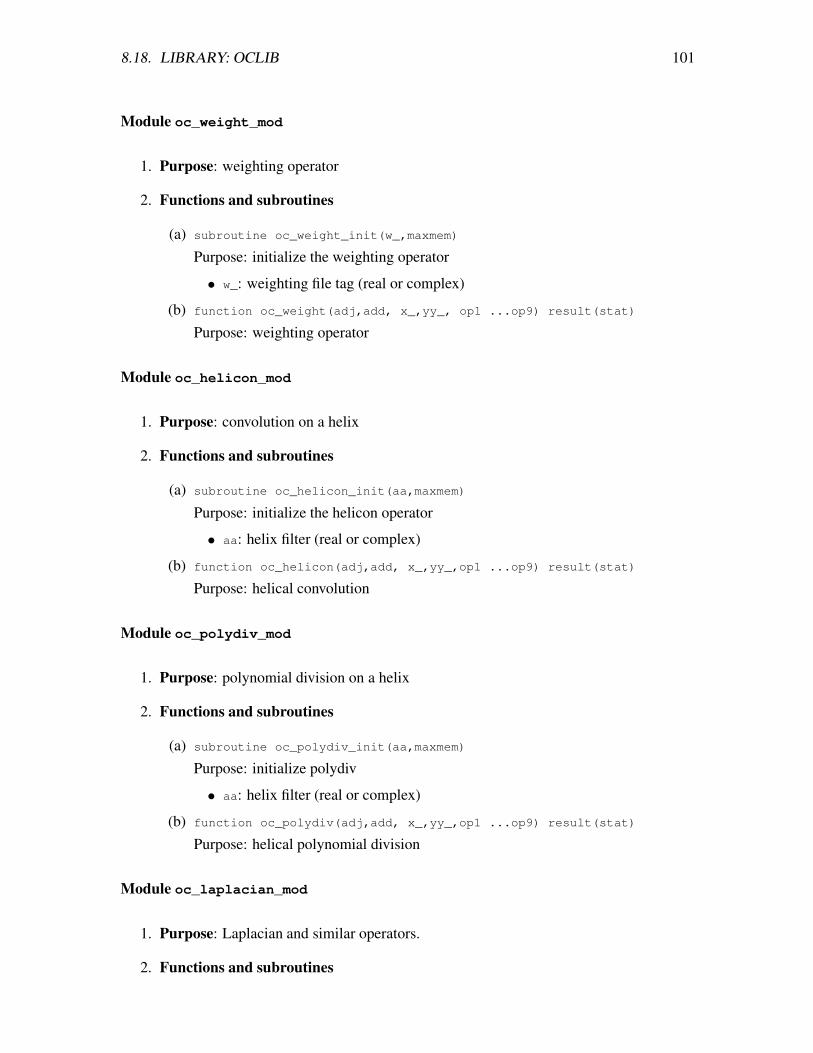
8.18. LIBRARY: OCLIB 101
Module oc_weight_mod
1. Purpose: weighting operator
2. Functions and subroutines
(a) subroutine oc_weight_init(w_,maxmem)
Purpose: initialize the weighting operator
• w_: weighting file tag (real or complex)
(b) function oc_weight(adj,add, x_,yy_, op1 ...op9) result(stat)
Purpose: weighting operator
Module oc_helicon_mod
1. Purpose: convolution on a helix
2. Functions and subroutines
(a) subroutine oc_helicon_init(aa,maxmem)
Purpose: initialize the helicon operator
• aa: helix filter (real or complex)
(b) function oc_helicon(adj,add, x_,yy_,op1 ...op9) result(stat)
Purpose: helical convolution
Module oc_polydiv_mod
1. Purpose: polynomial division on a helix
2. Functions and subroutines
(a) subroutine oc_polydiv_init(aa,maxmem)
Purpose: initialize polydiv
• aa: helix filter (real or complex)
(b) function oc_polydiv(adj,add, x_,yy_,op1 ...op9) result(stat)
Purpose: helical polynomial division
Module oc_laplacian_mod
1. Purpose: Laplacian and similar operators.
2. Functions and subroutines
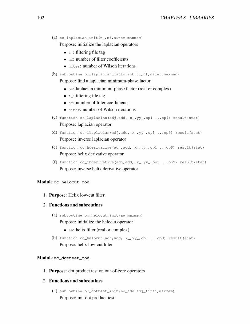
102 CHAPTER 8. LIBRARIES
(a) oc_laplacian_init(t_,nf,niter,maxmem)
Purpose: initialize the laplacian operators
• t_: filtering file tag• nf: number of filter coefficients• niter: number of Wilson iterations
(b) subroutine oc_laplacian_factor(bb,t_,nf,niter,maxmem)
Purpose: find a laplacian minimum-phase factor
• bb: laplacian minimum-phase factor (real or complex)• t_: filtering file tag• nf: number of filter coefficients• niter: number of Wilson iterations
(c) function oc_laplacian(adj,add, x_,yy_,op1 ...op9) result(stat)
Purpose: laplacian operator
(d) function oc_ilaplacian(adj,add, x_,yy_,op1 ...op9) result(stat)
Purpose: inverse laplacian operator
(e) function oc_hderivative(adj,add, x_,yy_,op1 ...op9) result(stat)
Purpose: helix derivative operator
(f) function oc_ihderivative(adj,add, x_,yy_,op1 ...op9) result(stat)
Purpose: inverse helix derivative operator
Module oc_helocut_mod
1. Purpose: Helix low-cut filter
2. Functions and subroutines
(a) subroutine oc_helocut_init(aa,maxmem)
Purpose: initialize the helocut operator
• aa: helix filter (real or complex)
(b) function oc_helocut(adj,add, x_,yy_,op1 ...op9) result(stat)
Purpose: helix low-cut filter
Module oc_dottest_mod
1. Purpose: dot product test on out-of-core operators
2. Functions and subroutines
(a) subroutine oc_dottest_init(no_add,adj_first,maxmem)
Purpose: init dot product test

8.18. LIBRARY: OCLIB 103
• no_add: skip DP test for add=.true.• adj_first: start DP test with the adjoint
(b) subroutine oc_dottest(oper, x_,yy_,op1 ...op9)
Purpose: dot product test
• oper: out-of-core operator
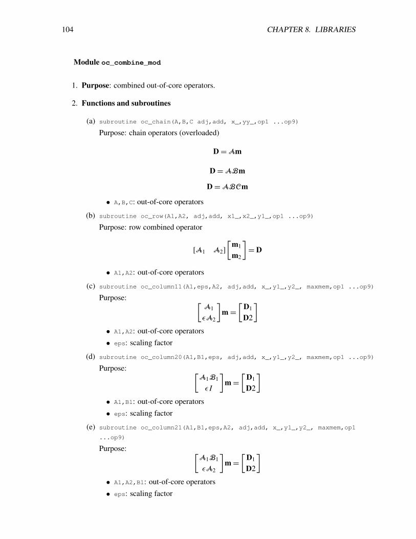
104 CHAPTER 8. LIBRARIES
Module oc_combine_mod
1. Purpose: combined out-of-core operators.
2. Functions and subroutines
(a) subroutine oc_chain(A,B,C adj,add, x_,yy_,op1 ...op9)
Purpose: chain operators (overloaded)
D=Am
D=ABm
D=ABCm
• A,B,C: out-of-core operators
(b) subroutine oc_row(A1,A2, adj,add, x1_,x2_,y1_,op1 ...op9)
Purpose: row combined operator
[A1 A2][
m1
m2
]
= D
• A1,A2: out-of-core operators
(c) subroutine oc_column11(A1,eps,A2, adj,add, x_,y1_,y2_, maxmem,op1 ...op9)
Purpose:[
A1
εA2
]
m=[
D1
D2
]
• A1,A2: out-of-core operators• eps: scaling factor
(d) subroutine oc_column20(A1,B1,eps, adj,add, x_,y1_,y2_, maxmem,op1 ...op9)
Purpose:[
A1B1
ε I
]
m=[
D1
D2
]
• A1,B1: out-of-core operators• eps: scaling factor
(e) subroutine oc_column21(A1,B1,eps,A2, adj,add, x_,y1_,y2_, maxmem,op1
...op9)
Purpose:[
A1B1
εA2
]
m=[
D1
D2
]
• A1,A2,B1: out-of-core operators• eps: scaling factor

8.18. LIBRARY: OCLIB 105
(f) subroutine oc_column30(A1,B1,C1,eps, adj,add, x_,y1_,y2_, maxmem,op1
...op9)
Purpose:[
A1B1C1
ε I
]
m=[
D1
D2
]
• A1,B1,C1,: out-of-core operators• eps: scaling factor
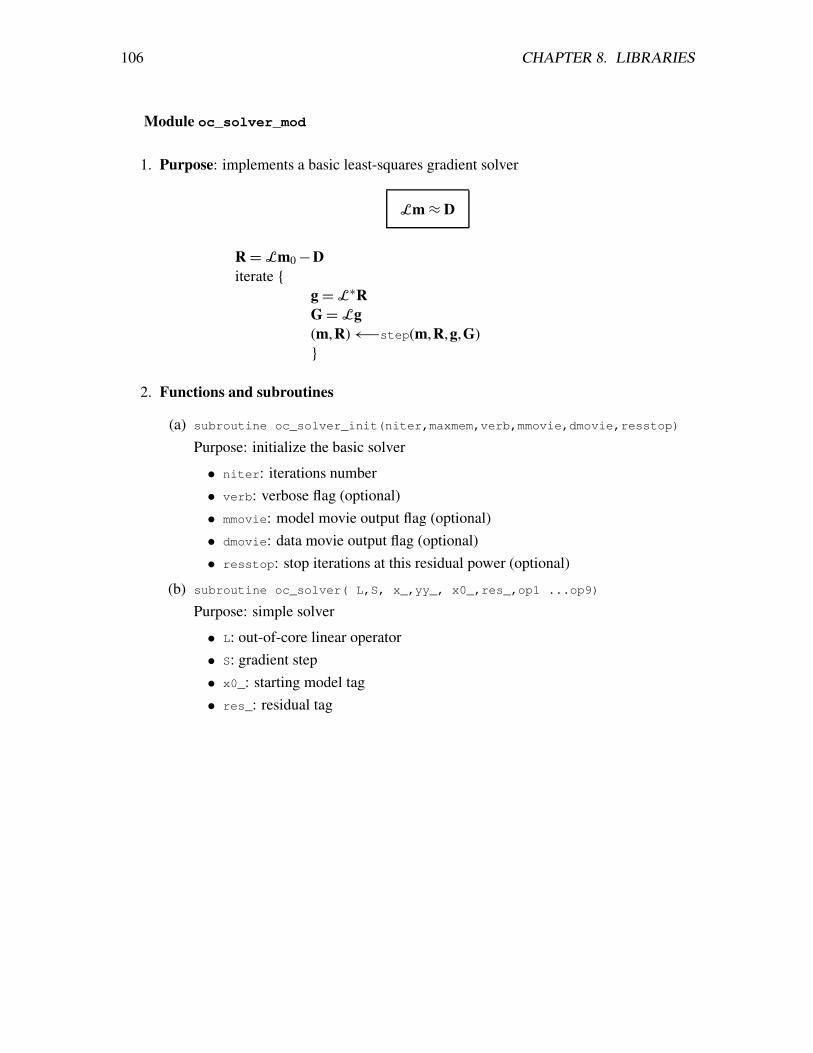
106 CHAPTER 8. LIBRARIES
Module oc_solver_mod
1. Purpose: implements a basic least-squares gradient solver
Lm≈ D
R=Lm0−Diterate {
g=L∗R
G=Lg(m,R)←−step(m,R,g,G)}
2. Functions and subroutines
(a) subroutine oc_solver_init(niter,maxmem,verb,mmovie,dmovie,resstop)
Purpose: initialize the basic solver
• niter: iterations number• verb: verbose flag (optional)• mmovie: model movie output flag (optional)• dmovie: data movie output flag (optional)• resstop: stop iterations at this residual power (optional)
(b) subroutine oc_solver( L,S, x_,yy_, x0_,res_,op1 ...op9)
Purpose: simple solver
• L: out-of-core linear operator• S: gradient step• x0_: starting model tag• res_: residual tag
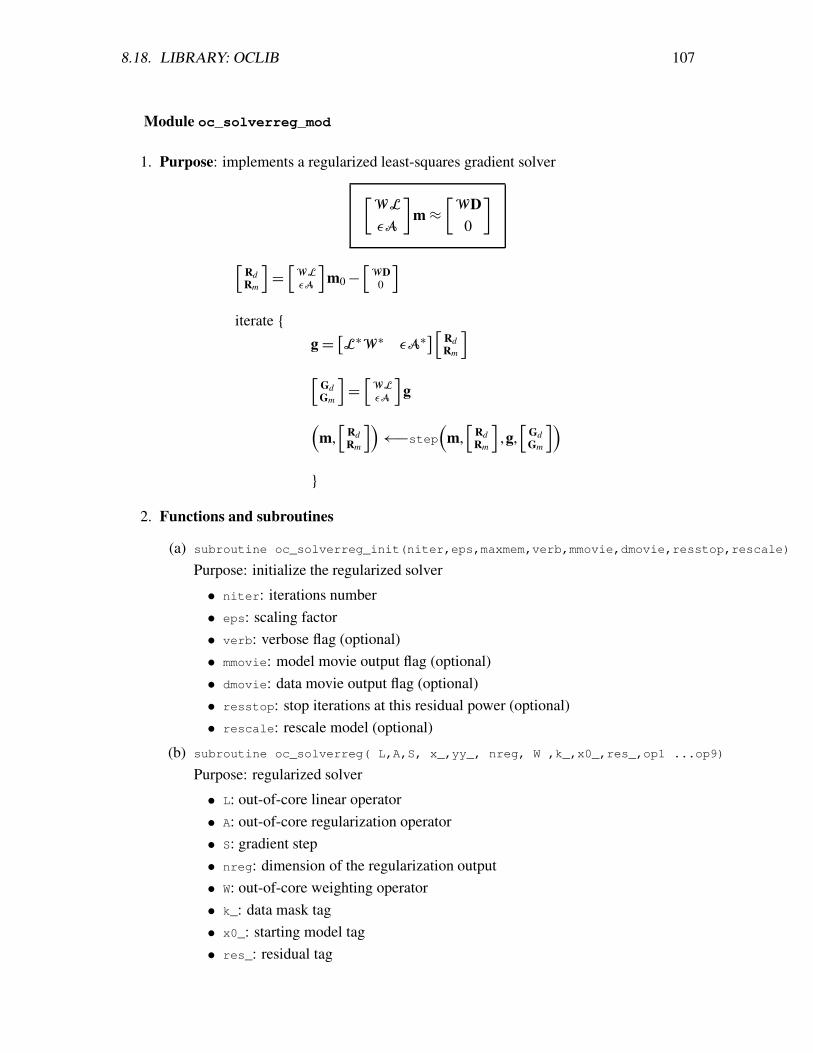
8.18. LIBRARY: OCLIB 107
Module oc_solverreg_mod
1. Purpose: implements a regularized least-squares gradient solver
[
WL
εA
]
m≈[
WD0
]
[
RdRm
]
=[
WL
εA
]
m0−[
WD0
]
iterate {
g=[
L∗W∗ εA∗
]
[
RdRm
]
[
GdGm
]
=[
WL
εA
]
g
(
m,[
RdRm
])
←−step(
m,[
RdRm
]
,g,[
GdGm
])
}
2. Functions and subroutines
(a) subroutine oc_solverreg_init(niter,eps,maxmem,verb,mmovie,dmovie,resstop,rescale)
Purpose: initialize the regularized solver
• niter: iterations number• eps: scaling factor• verb: verbose flag (optional)• mmovie: model movie output flag (optional)• dmovie: data movie output flag (optional)• resstop: stop iterations at this residual power (optional)• rescale: rescale model (optional)
(b) subroutine oc_solverreg( L,A,S, x_,yy_, nreg, W ,k_,x0_,res_,op1 ...op9)
Purpose: regularized solver
• L: out-of-core linear operator• A: out-of-core regularization operator• S: gradient step• nreg: dimension of the regularization output• W: out-of-core weighting operator• k_: data mask tag• x0_: starting model tag• res_: residual tag
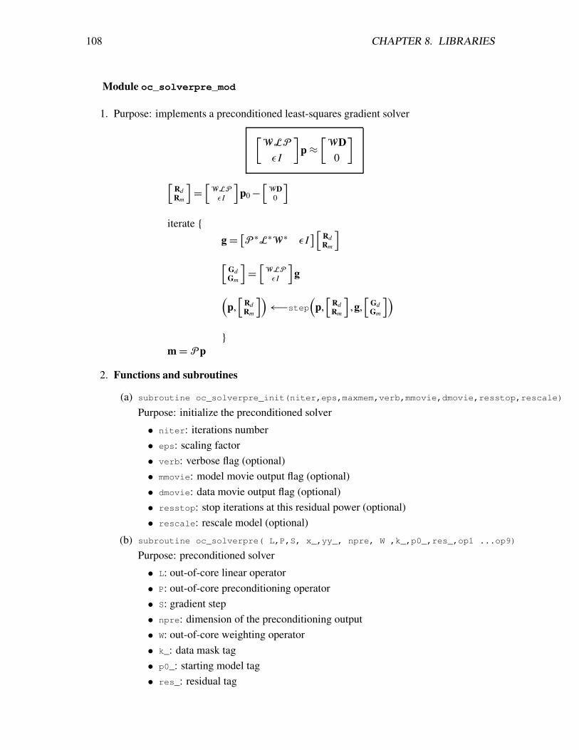
108 CHAPTER 8. LIBRARIES
Module oc_solverpre_mod
1. Purpose: implements a preconditioned least-squares gradient solver
[
WLP
ε I
]
p≈[
WD0
]
[
RdRm
]
=[
WLP
ε I
]
p0−[
WD0
]
iterate {
g=[
P∗L∗W∗ ε I
]
[
RdRm
]
[
GdGm
]
=[
WLP
ε I
]
g
(
p,[
RdRm
])
←−step(
p,[
RdRm
]
,g,[
GdGm
])
}m= Pp
2. Functions and subroutines
(a) subroutine oc_solverpre_init(niter,eps,maxmem,verb,mmovie,dmovie,resstop,rescale)
Purpose: initialize the preconditioned solver
• niter: iterations number• eps: scaling factor• verb: verbose flag (optional)• mmovie: model movie output flag (optional)• dmovie: data movie output flag (optional)• resstop: stop iterations at this residual power (optional)• rescale: rescale model (optional)
(b) subroutine oc_solverpre( L,P,S, x_,yy_, npre, W ,k_,p0_,res_,op1 ...op9)
Purpose: preconditioned solver
• L: out-of-core linear operator• P: out-of-core preconditioning operator• S: gradient step• npre: dimension of the preconditioning output• W: out-of-core weighting operator• k_: data mask tag• p0_: starting model tag• res_: residual tag
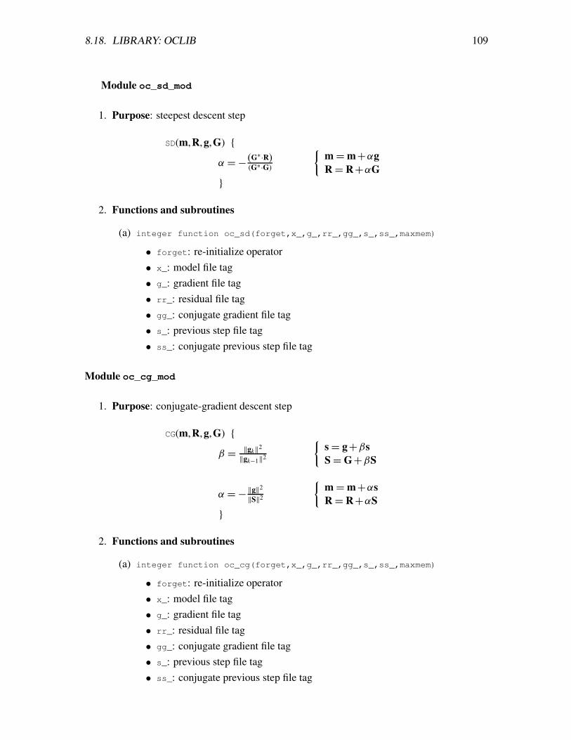
8.18. LIBRARY: OCLIB 109
Module oc_sd_mod
1. Purpose: steepest descent step
SD(m,R,g,G) {
α =− (G∗·R)(G∗·G)
{
m=m+αgR= R+αG
}
2. Functions and subroutines
(a) integer function oc_sd(forget,x_,g_,rr_,gg_,s_,ss_,maxmem)
• forget: re-initialize operator• x_: model file tag• g_: gradient file tag• rr_: residual file tag• gg_: conjugate gradient file tag• s_: previous step file tag• ss_: conjugate previous step file tag
Module oc_cg_mod
1. Purpose: conjugate-gradient descent step
CG(m,R,g,G) {
β = ‖gk‖2‖gk−1‖2
{
s= g+βsS=G+βS
α =− ‖g‖2
‖S‖2
{
m=m+αsR= R+αS
}
2. Functions and subroutines
(a) integer function oc_cg(forget,x_,g_,rr_,gg_,s_,ss_,maxmem)
• forget: re-initialize operator• x_: model file tag• g_: gradient file tag• rr_: residual file tag• gg_: conjugate gradient file tag• s_: previous step file tag• ss_: conjugate previous step file tag
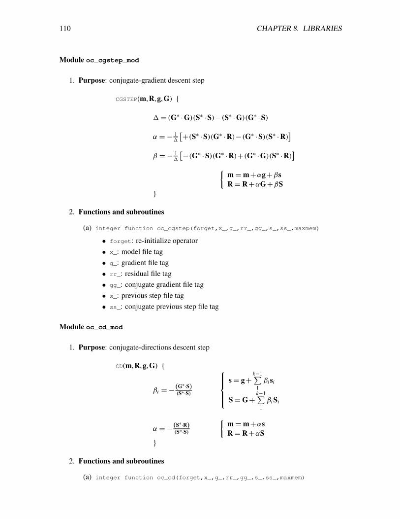
110 CHAPTER 8. LIBRARIES
Module oc_cgstep_mod
1. Purpose: conjugate-gradient descent step
CGSTEP(m,R,g,G) {
1= (G∗ ·G) (S∗ ·S)− (S∗ ·G) (G∗ ·S)
α =− 11
[
+ (S∗ ·S) (G∗ ·R)− (G∗ ·S) (S∗ ·R)]
β =− 11
[
− (G∗ ·S) (G∗ ·R)+ (G∗ ·G) (S∗ ·R)]
{
m=m+αg+βsR= R+αG+βS
}
2. Functions and subroutines
(a) integer function oc_cgstep(forget,x_,g_,rr_,gg_,s_,ss_,maxmem)
• forget: re-initialize operator• x_: model file tag• g_: gradient file tag• rr_: residual file tag• gg_: conjugate gradient file tag• s_: previous step file tag• ss_: conjugate previous step file tag
Module oc_cd_mod
1. Purpose: conjugate-directions descent step
CD(m,R,g,G) {
βi =− (G∗·S)(S∗·S)
s= g+k−1∑
1βi si
S=G+k−1∑
1βi Si
α =− (S∗·R)(S∗·S)
{
m=m+αsR= R+αS
}
2. Functions and subroutines
(a) integer function oc_cd(forget,x_,g_,rr_,gg_,s_,ss_,maxmem)
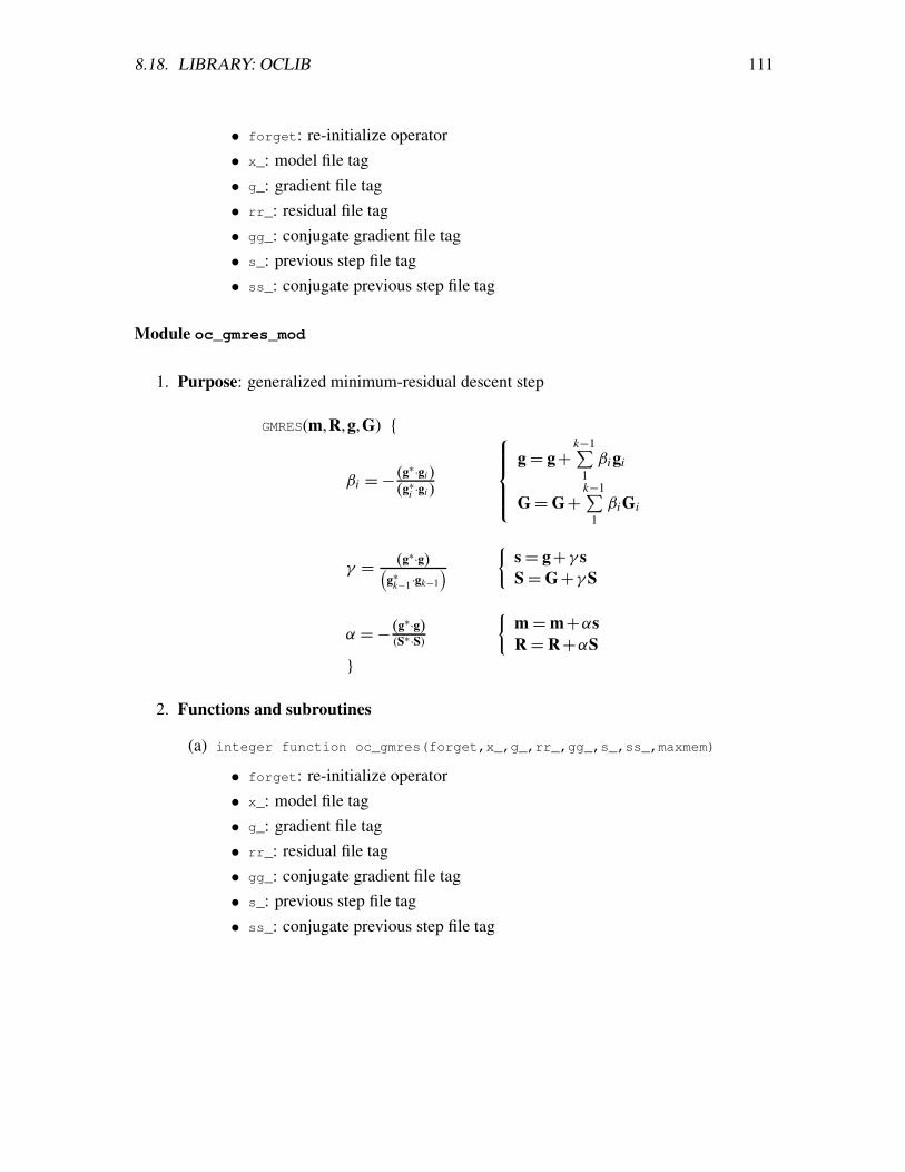
8.18. LIBRARY: OCLIB 111
• forget: re-initialize operator• x_: model file tag• g_: gradient file tag• rr_: residual file tag• gg_: conjugate gradient file tag• s_: previous step file tag• ss_: conjugate previous step file tag
Module oc_gmres_mod
1. Purpose: generalized minimum-residual descent step
GMRES(m,R,g,G) {
βi =− (g∗·gi)(g∗i ·gi)
g= g+k−1∑
1βi gi
G=G+k−1∑
1βi Gi
γ = (g∗·g)(
g∗k−1 ·gk−1
)
{
s= g+γ sS=G+γ S
α =− (g∗·g)(S∗·S)
{
m=m+αsR= R+αS
}
2. Functions and subroutines
(a) integer function oc_gmres(forget,x_,g_,rr_,gg_,s_,ss_,maxmem)
• forget: re-initialize operator• x_: model file tag• g_: gradient file tag• rr_: residual file tag• gg_: conjugate gradient file tag• s_: previous step file tag• ss_: conjugate previous step file tag
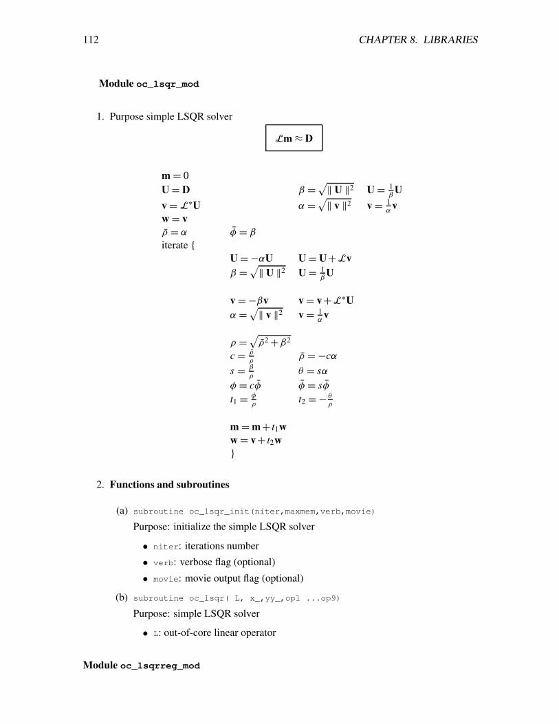
112 CHAPTER 8. LIBRARIES
Module oc_lsqr_mod
1. Purpose simple LSQR solver
Lm≈ D
m= 0U= D β =
√
‖ U ‖2 U= 1β
Uv=L
∗U α =√
‖ v ‖2 v= 1α
vw= vρ̄ = α φ̄ = β
iterate {U=−αU U= U+Lvβ =
√
‖ U ‖2 U= 1β
U
v=−βv v= v+L∗U
α =√
‖ v ‖2 v= 1α
v
ρ =√
ρ̄2+β2
c = ρ̄
ρρ̄ =−cα
s = β
ρθ = sα
φ = cφ̄ φ̄ = sφ̄t1 = φ
ρt2 =− θ
ρ
m=m+ t1ww= v+ t2w}
2. Functions and subroutines
(a) subroutine oc_lsqr_init(niter,maxmem,verb,movie)
Purpose: initialize the simple LSQR solver
• niter: iterations number
• verb: verbose flag (optional)
• movie: movie output flag (optional)
(b) subroutine oc_lsqr( L, x_,yy_,op1 ...op9)
Purpose: simple LSQR solver
• L: out-of-core linear operator
Module oc_lsqrreg_mod
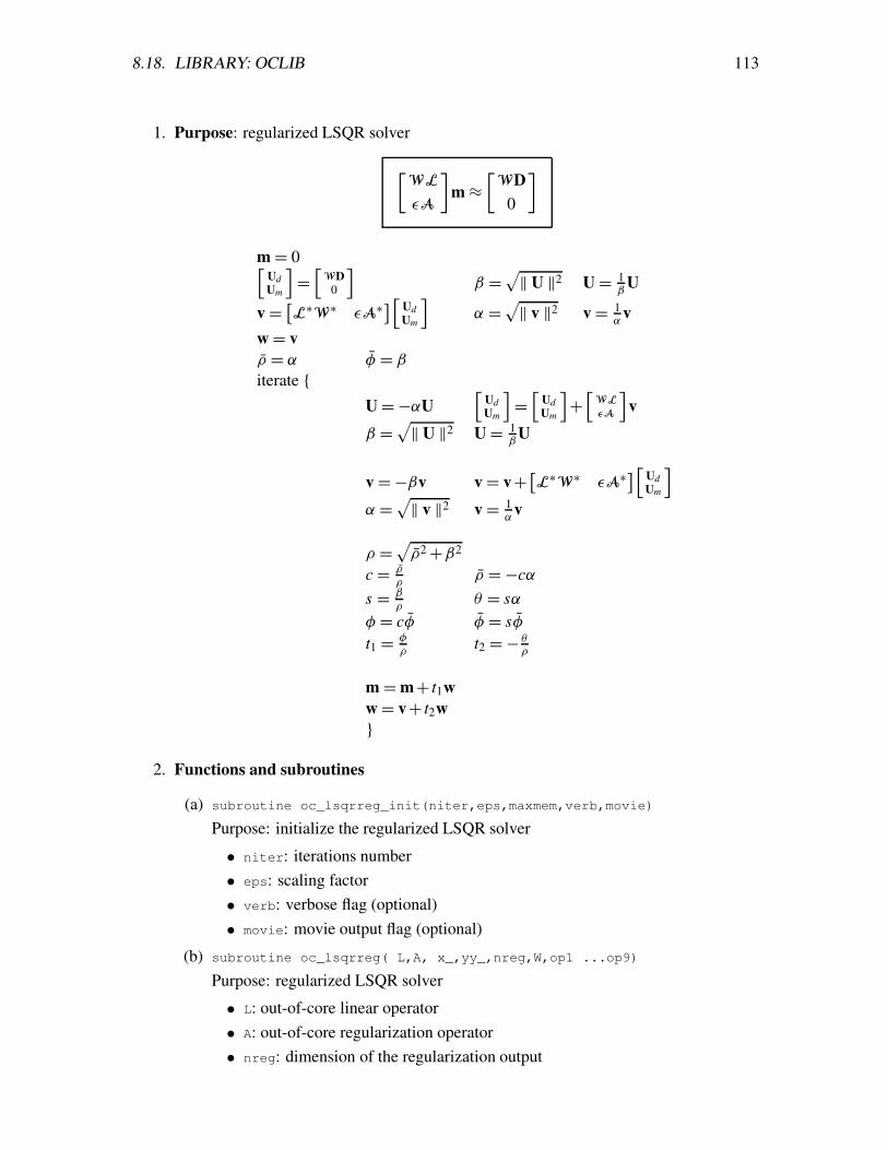
8.18. LIBRARY: OCLIB 113
1. Purpose: regularized LSQR solver
[
WL
εA
]
m≈[
WD0
]
m= 0[
UdUm
]
=[
WD0
]
β =√
‖ U ‖2 U= 1β
U
v=[
L∗W∗ εA∗
]
[
UdUm
]
α =√
‖ v ‖2 v= 1α
vw= vρ̄ = α φ̄ = β
iterate {
U=−αU[
UdUm
]
=[
UdUm
]
+[
WL
εA
]
v
β =√
‖ U ‖2 U= 1β
U
v=−βv v= v+[
L∗W∗ εA∗
]
[
UdUm
]
α =√
‖ v ‖2 v= 1α
v
ρ =√
ρ̄2+β2
c = ρ̄
ρρ̄ =−cα
s = β
ρθ = sα
φ = cφ̄ φ̄ = sφ̄t1 = φ
ρt2 =− θ
ρ
m=m+ t1ww= v+ t2w}
2. Functions and subroutines
(a) subroutine oc_lsqrreg_init(niter,eps,maxmem,verb,movie)
Purpose: initialize the regularized LSQR solver
• niter: iterations number• eps: scaling factor• verb: verbose flag (optional)• movie: movie output flag (optional)
(b) subroutine oc_lsqrreg( L,A, x_,yy_,nreg,W,op1 ...op9)
Purpose: regularized LSQR solver
• L: out-of-core linear operator• A: out-of-core regularization operator• nreg: dimension of the regularization output
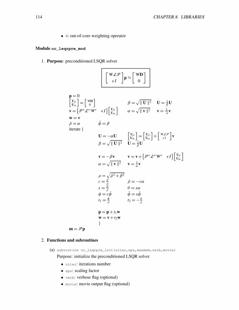
114 CHAPTER 8. LIBRARIES
• W: out-of-core weighting operator
Module oc_lsqrpre_mod
1. Purpose: preconditioned LSQR solver
[
WLP
ε I
]
p≈[
WD0
]
p= 0[
UdUm
]
=[
WD0
]
β =√
‖ U ‖2 U= 1β
U
v=[
P∗L∗W∗ ε I
]
[
UdUm
]
α =√
‖ v ‖2 v= 1a v
w= vρ̄ = α φ̄ = β
iterate {
U=−αU[
UdUm
]
=[
UdUm
]
+[
WLP
ε I
]
v
β =√
‖ U ‖2 U= 1β
U
v=−βv v= v+[
P∗L∗W∗ ε I
]
[
UdUm
]
α =√
‖ v ‖2 v= 1α
v
ρ =√
ρ̄2+β2
c = ρ̄
ρρ̄ =−cα
s = β
ρθ = sα
φ = cφ̄ φ̄ = sφ̄t1 = φ
ρt2 =− θ
ρ
p= p+ t1ww= v+ t2w}
m= Pp
2. Functions and subroutines
(a) subroutine oc_lsqrpre_init(niter,eps,maxmem,verb,movie)
Purpose: initialize the preconditioned LSQR solver
• niter: iterations number• eps: scaling factor• verb: verbose flag (optional)• movie: movie output flag (optional)

8.18. LIBRARY: OCLIB 115
(b) subroutine oc_lsqrpre( L,P, x_,yy_,npre,W,op1 ...op9)
Purpose: preconditioned LSQR solver
• L: out-of-core linear operator• P: out-of-core preconditioning operator• npre: dimension of the preconditioning output• W: out-of-core weighting operator

116 CHAPTER 8. LIBRARIES

Chapter 9
Writing a program
To get the most out of SEPlib, you need to be able to write programs that will read andwrite SEPlib datasets. This chapter contains examples of how to write several different typesof SEPlib programs. Each section represents how to program a simple task in one or morecomputer languages.
9.1 How to write a SEPlib program
This section contains examples of a simple scaling program in several languages. The exam-ples show:
• How to obtain information from the history file and from a parameter file.
• How to read in data.
• Scaling of the data.
• How to write out data.
9.1.1 Language: C
Most of SEPlib is written in C, so this can be considered the classic example.
/*$
Self-doc area
Scale_c.x
Usage
Scale_c.x <input.H scale= >output.H
Input Parameters:
117
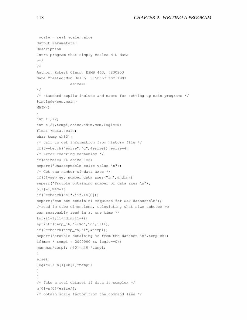
118 CHAPTER 9. WRITING A PROGRAM
scale - real scale value
Output Parameters:
Description
Intro program that simply scales N-D data
>*/
/*
Author: Robert Clapp, ESMB 463, 7230253
Date Created:Mon Jul 5 8:50:57 PDT 1997
esize=1
*/
/* standard seplib include and macro for setting up main programs */
#include<sep.main>
MAIN()
{
int i1,i2;
int n[2],tempi,esize,ndim,mem,logic=0;
float *data,scale;
char temp_ch[3];
/* call to get information from history file */
if(0==hetch("esize","d",&esize)) esize=4;
/* Error checking mechanism */
if(esize!=4 && esize !=8)
seperr("Unacceptable esize value \n");
/* Get the number of data axes */
if(0!=sep_get_number_data_axes("in",&ndim))
seperr("Trouble obtaining number of data axes \n");
n[1]=1;mem=1;
if(0==hetch("n1","i",&n[0]))
seperr("can not obtain n1 required for SEP datasets\n");
/*read in cube dimensions, calculating what size subcube we
can reasonably read in at one time */
for(i1=1;i1<ndim;i1++){
sprintf(temp_ch,"%c%d",’n’,i1+1);
if(0==hetch(temp_ch,"i",&tempi))
seperr("trouble obtaining %s from the dataset \n",temp_ch);
if(mem * tempi < 2000000 && logic==0){
mem=mem*tempi; n[0]=n[0]*tempi;
}
else{
logic=1; n[1]=n[1]*tempi;
}
}
/* fake a real dataset if data is complex */
n[0]=n[0]*esize/4;
/* obtain scale factor from the command line */
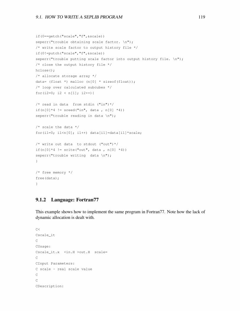
9.1. HOW TO WRITE A SEPLIB PROGRAM 119
if(0==getch("scale","f",&scale))
seperr("trouble obtaining scale factor. \n");
/* write scale factor to output history file */
if(0!=putch("scale","f",&scale))
seperr("trouble putting scale factor into output history file. \n");
/* close the output history file */
hclose();
/* allocate storage array */
data= (float *) malloc (n[0] * sizeof(float));
/* loop over calculated subcubes */
for(i2=0; i2 < n[1]; i2++){
/* read in data from stdin ("in")*/
if(n[0]*4 != sreed("in", data , n[0] *4))
seperr("trouble reading in data \n");
/* scale the data */
for(i1=0; i1<n[0]; i1++) data[i1]=data[i1]*scale;
/* write out data to stdout ("out")*/
if(n[0]*4 != srite("out", data , n[0] *4))
seperr("trouble writing data \n");
}
/* free memory */
free(data);
}
9.1.2 Language: Fortran77
This example shows how to implement the same program in Fortran77. Note how the lack ofdynamic allocation is dealt with.
C<
Cscale_it
C
CUsage:
Cscale_it.x <in.H >out.H scale=
C
CInput Parameters:
C scale - real scale value
C
C
CDescription:
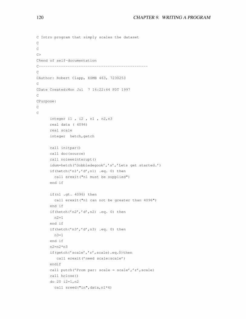
120 CHAPTER 9. WRITING A PROGRAM
C Intro program that simply scales the dataset
C
C
C>
C%end of self-documentation
C-------------------------------------------------
C
CAuthor: Robert Clapp, ESMB 463, 7230253
C
CDate Created:Mon Jul 7 16:22:44 PDT 1997
C
CPurpose:
C
C
integer i1 , i2 , n1 , n2,n3
real data ( 4096)
real scale
integer hetch,getch
call initpar()
call doc(source)
call noieeeinterupt()
idum=hetch(’Gobbledegook’,’s’,’Lets get started.’)
if(hetch(’n1’,’d’,n1) .eq. 0) then
call erexit("n1 must be supplied")
end if
if(n1 .gt. 4096) then
call erexit("n1 can not be greater than 4096")
end if
if(hetch(’n2’,’d’,n2) .eq. 0) then
n2=1
end if
if(hetch(’n3’,’d’,n3) .eq. 0) then
n3=1
end if
n2=n2*n3
if(getch(’scale’,’r’,scale).eq.0)then
call erexit(’need scale:scale’)
endif
call putch(’From par: scale = scale’,’r’,scale)
call hclose()
do 20 i2=1,n2
call sreed("in",data,n1*4)
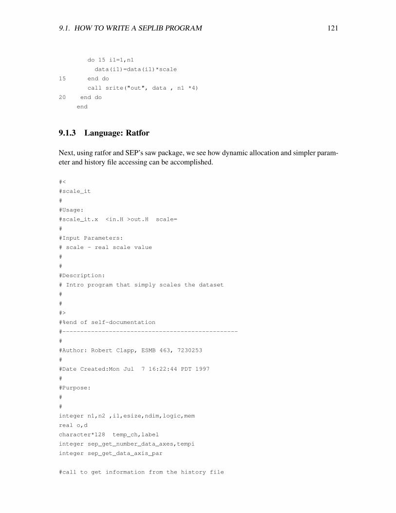
9.1. HOW TO WRITE A SEPLIB PROGRAM 121
do 15 i1=1,n1
data(i1)=data(i1)*scale
15 end do
call srite("out", data , n1 *4)
20 end do
end
9.1.3 Language: Ratfor
Next, using ratfor and SEP’s saw package, we see how dynamic allocation and simpler param-eter and history file accessing can be accomplished.
#<
#scale_it
#
#Usage:
#scale_it.x <in.H >out.H scale=
#
#Input Parameters:
# scale - real scale value
#
#
#Description:
# Intro program that simply scales the dataset
#
#
#>
#%end of self-documentation
#-------------------------------------------------
#
#Author: Robert Clapp, ESMB 463, 7230253
#
#Date Created:Mon Jul 7 16:22:44 PDT 1997
#
#Purpose:
#
#
integer n1,n2 ,i1,esize,ndim,logic,mem
real o,d
character*128 temp_ch,label
integer sep_get_number_data_axes,tempi
integer sep_get_data_axis_par
#call to get information from the history file
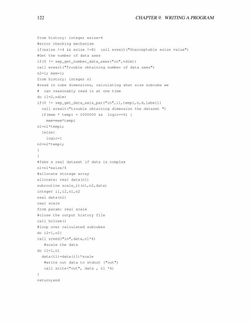
122 CHAPTER 9. WRITING A PROGRAM
from history: integer esize=4
#error checking mechanism
if(esize !=4 && esize !=8) call erexit("Unacceptable esize value")
#Get the number of data axes
if(0 != sep_get_number_data_axes("in",ndim))
call erexit("Trouble obtaining number of data axes")
n2=1; mem=1;
from history: integer n1
#read in cube dimensions, calculating what size subcube we
# can reasonably read in at one time
do i1=2,ndim{
if(0 != sep_get_data_axis_par("in",i1,tempi,o,d,label))
call erexit("trouble obtaining dimension the dataset ")
if(mem * tempi < 2000000 && logic==0) {
mem=mem*tempi
n1=n1*tempi;
}else{
logic=1
n2=n2*tempi;
}
}
#fake a real dataset if data is complex
n1=n1*esize/4
#allocate storage array
allocate: real data(n1)
subroutine scale_it(n1,n2,data)
integer i1,i2,n1,n2
real data(n1)
real scale
from param: real scale
#close the output history file
call hclose()
#loop over calculated subcubes
do i2=1,n2{
call sreed("in",data,n1*4)
#scale the data
do i1=1,n1
data(i1)=data(i1)*scale
#write out data to stdout ("out")
call srite("out", data , n1 *4)
}
return;end
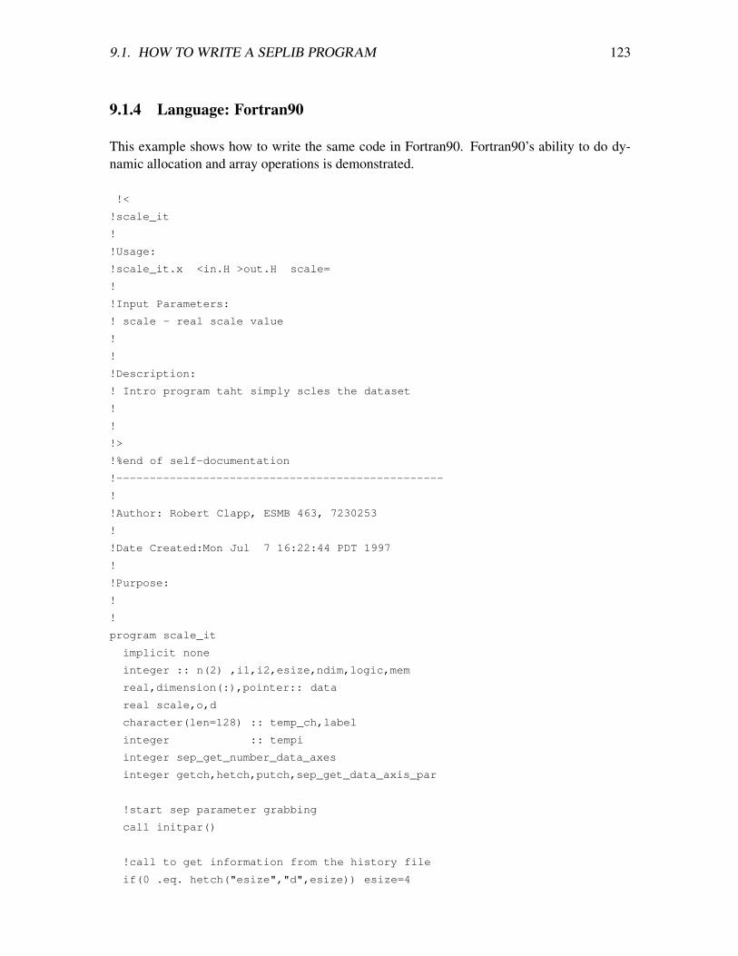
9.1. HOW TO WRITE A SEPLIB PROGRAM 123
9.1.4 Language: Fortran90
This example shows how to write the same code in Fortran90. Fortran90’s ability to do dy-namic allocation and array operations is demonstrated.
!<
!scale_it
!
!Usage:
!scale_it.x <in.H >out.H scale=
!
!Input Parameters:
! scale - real scale value
!
!
!Description:
! Intro program taht simply scles the dataset
!
!
!>
!%end of self-documentation
!-------------------------------------------------
!
!Author: Robert Clapp, ESMB 463, 7230253
!
!Date Created:Mon Jul 7 16:22:44 PDT 1997
!
!Purpose:
!
!
program scale_it
implicit none
integer :: n(2) ,i1,i2,esize,ndim,logic,mem
real,dimension(:),pointer:: data
real scale,o,d
character(len=128) :: temp_ch,label
integer :: tempi
integer sep_get_number_data_axes
integer getch,hetch,putch,sep_get_data_axis_par
!start sep parameter grabbing
call initpar()
!call to get information from the history file
if(0 .eq. hetch("esize","d",esize)) esize=4
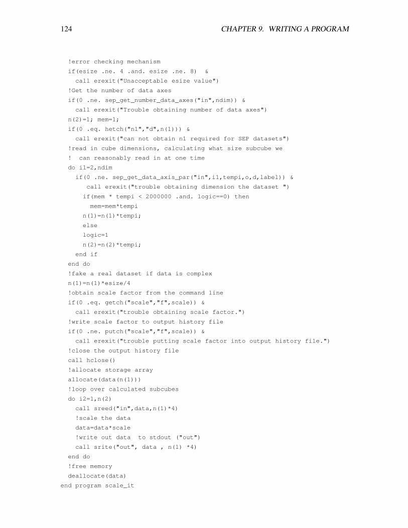
124 CHAPTER 9. WRITING A PROGRAM
!error checking mechanism
if(esize .ne. 4 .and. esize .ne. 8) &
call erexit("Unacceptable esize value")
!Get the number of data axes
if(0 .ne. sep_get_number_data_axes("in",ndim)) &
call erexit("Trouble obtaining number of data axes")
n(2)=1; mem=1;
if(0 .eq. hetch("n1","d",n(1))) &
call erexit("can not obtain n1 required for SEP datasets")
!read in cube dimensions, calculating what size subcube we
! can reasonably read in at one time
do i1=2,ndim
if(0 .ne. sep_get_data_axis_par("in",i1,tempi,o,d,label)) &
call erexit("trouble obtaining dimension the dataset ")
if(mem * tempi < 2000000 .and. logic==0) then
mem=mem*tempi
n(1)=n(1)*tempi;
else
logic=1
n(2)=n(2)*tempi;
end if
end do
!fake a real dataset if data is complex
n(1)=n(1)*esize/4
!obtain scale factor from the command line
if(0 .eq. getch("scale","f",scale)) &
call erexit("trouble obtaining scale factor.")
!write scale factor to output history file
if(0 .ne. putch("scale","f",scale)) &
call erexit("trouble putting scale factor into output history file.")
!close the output history file
call hclose()
!allocate storage array
allocate(data(n(1)))
!loop over calculated subcubes
do i2=1,n(2)
call sreed("in",data,n(1)*4)
!scale the data
data=data*scale
!write out data to stdout ("out")
call srite("out", data , n(1) *4)
end do
!free memory
deallocate(data)
end program scale_it
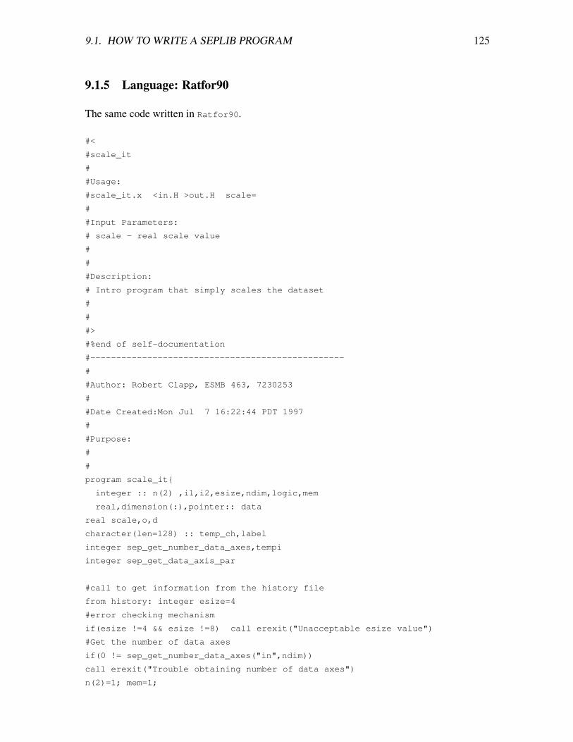
9.1. HOW TO WRITE A SEPLIB PROGRAM 125
9.1.5 Language: Ratfor90
The same code written in Ratfor90.
#<
#scale_it
#
#Usage:
#scale_it.x <in.H >out.H scale=
#
#Input Parameters:
# scale - real scale value
#
#
#Description:
# Intro program that simply scales the dataset
#
#
#>
#%end of self-documentation
#-------------------------------------------------
#
#Author: Robert Clapp, ESMB 463, 7230253
#
#Date Created:Mon Jul 7 16:22:44 PDT 1997
#
#Purpose:
#
#
program scale_it{
integer :: n(2) ,i1,i2,esize,ndim,logic,mem
real,dimension(:),pointer:: data
real scale,o,d
character(len=128) :: temp_ch,label
integer sep_get_number_data_axes,tempi
integer sep_get_data_axis_par
#call to get information from the history file
from history: integer esize=4
#error checking mechanism
if(esize !=4 && esize !=8) call erexit("Unacceptable esize value")
#Get the number of data axes
if(0 != sep_get_number_data_axes("in",ndim))
call erexit("Trouble obtaining number of data axes")
n(2)=1; mem=1;
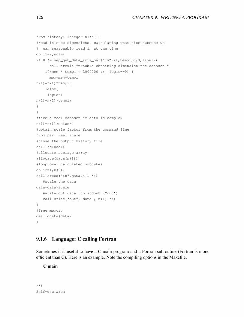
126 CHAPTER 9. WRITING A PROGRAM
from history: integer n1:n(1)
#read in cube dimensions, calculating what size subcube we
# can reasonably read in at one time
do i1=2,ndim{
if(0 != sep_get_data_axis_par("in",i1,tempi,o,d,label))
call erexit("trouble obtaining dimension the dataset ")
if(mem * tempi < 2000000 && logic==0) {
mem=mem*tempi
n(1)=n(1)*tempi;
}else{
logic=1
n(2)=n(2)*tempi;
}
}
#fake a real dataset if data is complex
n(1)=n(1)*esize/4
#obtain scale factor from the command line
from par: real scale
#close the output history file
call hclose()
#allocate storage array
allocate(data(n(1)))
#loop over calculated subcubes
do i2=1,n(2){
call sreed("in",data,n(1)*4)
#scale the data
data=data*scale
#write out data to stdout ("out")
call srite("out", data , n(1) *4)
}
#free memory
deallocate(data)
}
9.1.6 Language: C calling Fortran
Sometimes it is useful to have a C main program and a Fortran subroutine (Fortran is moreefficient than C). Here is an example. Note the compiling options in the Makefile.
C main
/*$
Self-doc area
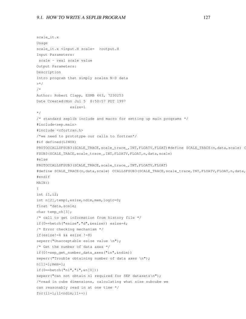
9.1. HOW TO WRITE A SEPLIB PROGRAM 127
scale_it.x
Usage
scale_it.x <input.H scale= >output.H
Input Parameters:
scale - real scale value
Output Parameters:
Description
Intro program that simply scales N-D data
>*/
/*
Author: Robert Clapp, ESMB 463, 7230253
Date Created:Mon Jul 5 8:50:57 PDT 1997
esize=1
*/
/* standard seplib include and macro for setting up main programs */
#include<sep.main>
#include <cfortran.h>
/*we need to prototype our calls to fortran*/
#if defined(LINUX)
PROTOCCALLSFSUB3(SCALE_TRACE,scale_trace_,INT,FLOATV,FLOAT)#define SCALE_TRACE(n,data,scale) CCALLS-
FSUB3(SCALE_TRACE,scale_trace_,INT,FLOATV,FLOAT,n,data,scale)
#else
PROTOCCALLSFSUB3(SCALE_TRACE,scale_trace_,INT,FLOATV,FLOAT)
#define SCALE_TRACE(n,data,scale) CCALLSFSUB3(SCALE_TRACE,scale_trace,INT,FLOATV,FLOAT,n,data,scale)
#endif
MAIN()
{
int i1,i2;
int n[2],tempi,esize,ndim,mem,logic=0;
float *data,scale;
char temp_ch[3];
/* call to get information from history file */
if(0==hetch("esize","d",&esize)) esize=4;
/* Error checking mechanism */
if(esize!=4 && esize !=8)
seperr("Unacceptable esize value \n");
/* Get the number of data axes */
if(0!=sep_get_number_data_axes("in",&ndim))
seperr("Trouble obtaining number of data axes \n");
n[1]=1;mem=1;
if(0==hetch("n1","i",&n[0]))
seperr("can not obtain n1 required for SEP datasets\n");
/*read in cube dimensions, calculating what size subcube we
can reasonably read in at one time */
for(i1=1;i1<ndim;i1++){
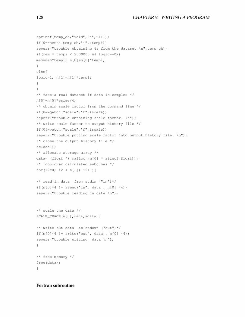
128 CHAPTER 9. WRITING A PROGRAM
sprintf(temp_ch,"%c%d",’n’,i1+1);
if(0==hetch(temp_ch,"i",&tempi))
seperr("trouble obtaining %s from the dataset \n",temp_ch);
if(mem * tempi < 2000000 && logic==0){
mem=mem*tempi; n[0]=n[0]*tempi;
}
else{
logic=1; n[1]=n[1]*tempi;
}
}
/* fake a real dataset if data is complex */
n[0]=n[0]*esize/4;
/* obtain scale factor from the command line */
if(0==getch("scale","f",&scale))
seperr("trouble obtaining scale factor. \n");
/* write scale factor to output history file */
if(0!=putch("scale","f",&scale))
seperr("trouble putting scale factor into output history file. \n");
/* close the output history file */
hclose();
/* allocate storage array */
data= (float *) malloc (n[0] * sizeof(float));
/* loop over calculated subcubes */
for(i2=0; i2 < n[1]; i2++){
/* read in data from stdin ("in")*/
if(n[0]*4 != sreed("in", data , n[0] *4))
seperr("trouble reading in data \n");
/* scale the data */
SCALE_TRACE(n[0],data,scale);
/* write out data to stdout ("out")*/
if(n[0]*4 != srite("out", data , n[0] *4))
seperr("trouble writing data \n");
}
/* free memory */
free(data);
}
Fortran subroutine
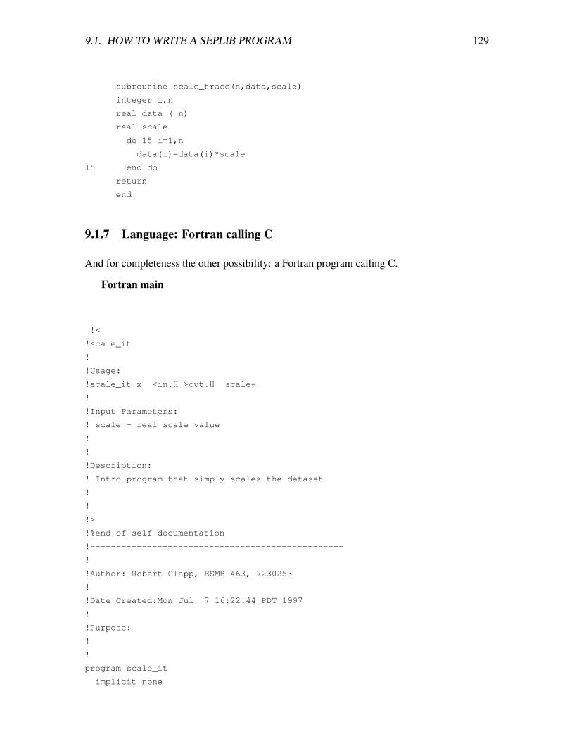
9.1. HOW TO WRITE A SEPLIB PROGRAM 129
subroutine scale_trace(n,data,scale)
integer i,n
real data ( n)
real scale
do 15 i=1,n
data(i)=data(i)*scale
15 end do
return
end
9.1.7 Language: Fortran calling C
And for completeness the other possibility: a Fortran program calling C.
Fortran main
!<
!scale_it
!
!Usage:
!scale_it.x <in.H >out.H scale=
!
!Input Parameters:
! scale - real scale value
!
!
!Description:
! Intro program that simply scales the dataset
!
!
!>
!%end of self-documentation
!-------------------------------------------------
!
!Author: Robert Clapp, ESMB 463, 7230253
!
!Date Created:Mon Jul 7 16:22:44 PDT 1997
!
!Purpose:
!
!
program scale_it
implicit none
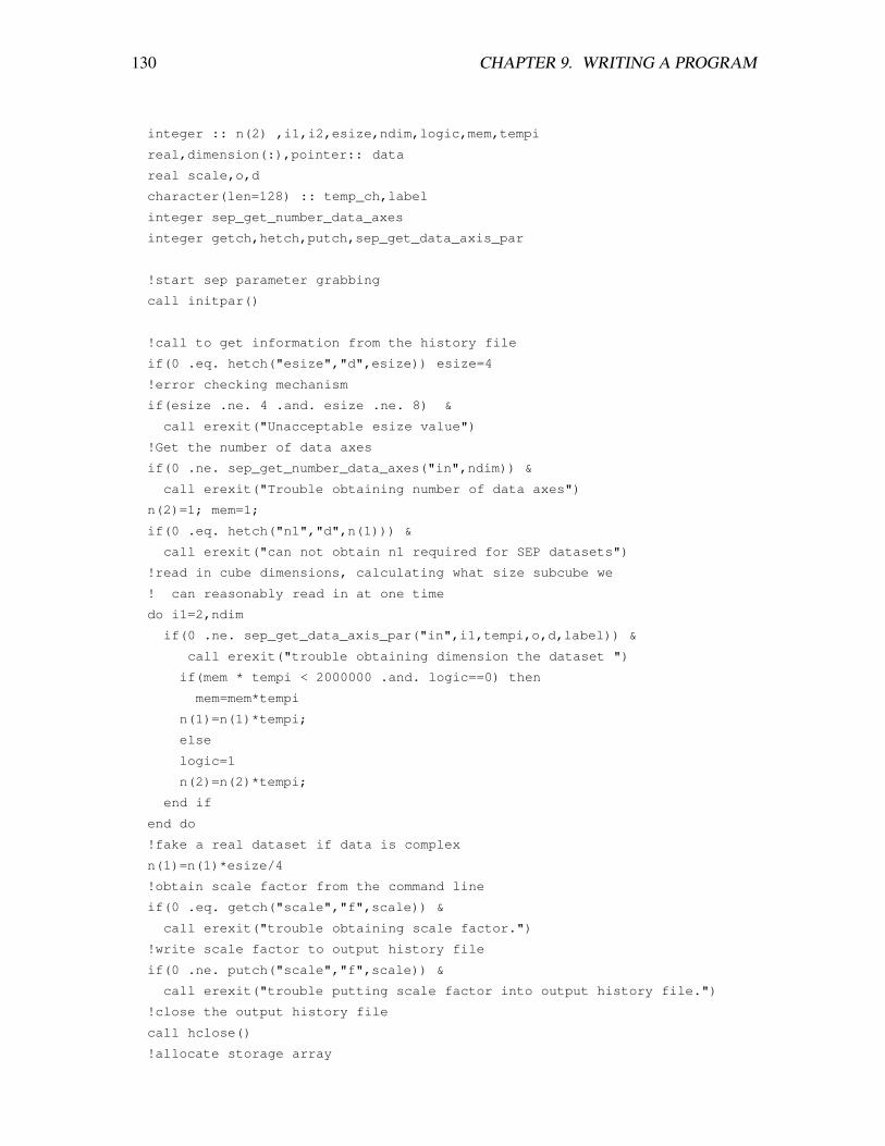
130 CHAPTER 9. WRITING A PROGRAM
integer :: n(2) ,i1,i2,esize,ndim,logic,mem,tempi
real,dimension(:),pointer:: data
real scale,o,d
character(len=128) :: temp_ch,label
integer sep_get_number_data_axes
integer getch,hetch,putch,sep_get_data_axis_par
!start sep parameter grabbing
call initpar()
!call to get information from the history file
if(0 .eq. hetch("esize","d",esize)) esize=4
!error checking mechanism
if(esize .ne. 4 .and. esize .ne. 8) &
call erexit("Unacceptable esize value")
!Get the number of data axes
if(0 .ne. sep_get_number_data_axes("in",ndim)) &
call erexit("Trouble obtaining number of data axes")
n(2)=1; mem=1;
if(0 .eq. hetch("n1","d",n(1))) &
call erexit("can not obtain n1 required for SEP datasets")
!read in cube dimensions, calculating what size subcube we
! can reasonably read in at one time
do i1=2,ndim
if(0 .ne. sep_get_data_axis_par("in",i1,tempi,o,d,label)) &
call erexit("trouble obtaining dimension the dataset ")
if(mem * tempi < 2000000 .and. logic==0) then
mem=mem*tempi
n(1)=n(1)*tempi;
else
logic=1
n(2)=n(2)*tempi;
end if
end do
!fake a real dataset if data is complex
n(1)=n(1)*esize/4
!obtain scale factor from the command line
if(0 .eq. getch("scale","f",scale)) &
call erexit("trouble obtaining scale factor.")
!write scale factor to output history file
if(0 .ne. putch("scale","f",scale)) &
call erexit("trouble putting scale factor into output history file.")
!close the output history file
call hclose()
!allocate storage array
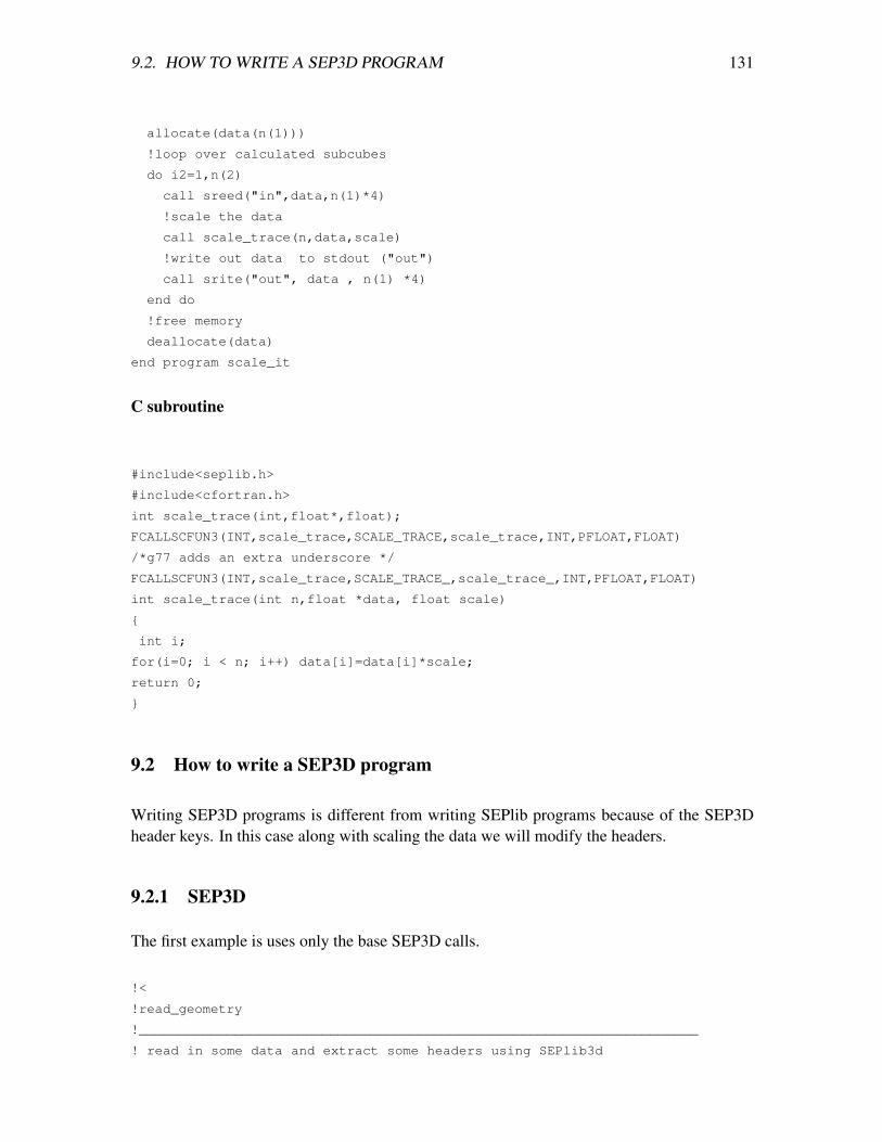
9.2. HOW TO WRITE A SEP3D PROGRAM 131
allocate(data(n(1)))
!loop over calculated subcubes
do i2=1,n(2)
call sreed("in",data,n(1)*4)
!scale the data
call scale_trace(n,data,scale)
!write out data to stdout ("out")
call srite("out", data , n(1) *4)
end do
!free memory
deallocate(data)
end program scale_it
C subroutine
#include<seplib.h>
#include<cfortran.h>
int scale_trace(int,float*,float);
FCALLSCFUN3(INT,scale_trace,SCALE_TRACE,scale_trace,INT,PFLOAT,FLOAT)
/*g77 adds an extra underscore */
FCALLSCFUN3(INT,scale_trace,SCALE_TRACE_,scale_trace_,INT,PFLOAT,FLOAT)
int scale_trace(int n,float *data, float scale)
{
int i;
for(i=0; i < n; i++) data[i]=data[i]*scale;
return 0;
}
9.2 How to write a SEP3D program
Writing SEP3D programs is different from writing SEPlib programs because of the SEP3Dheader keys. In this case along with scaling the data we will modify the headers.
9.2.1 SEP3D
The first example is uses only the base SEP3D calls.
!<
!read_geometry
!______________________________________________________________________
! read in some data and extract some headers using SEPlib3d
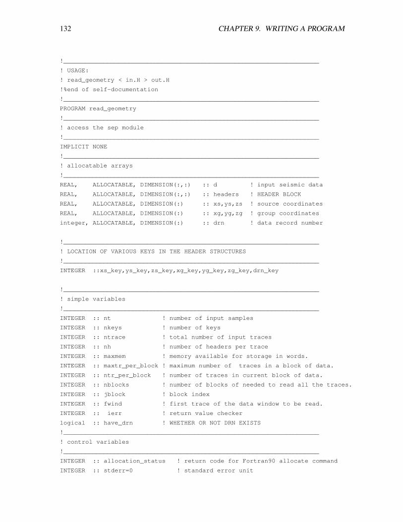
132 CHAPTER 9. WRITING A PROGRAM
!______________________________________________________________________
! USAGE:
! read_geometry < in.H > out.H
!%end of self-documentation
!______________________________________________________________________
PROGRAM read_geometry
!______________________________________________________________________
! access the sep module
!______________________________________________________________________
IMPLICIT NONE
!______________________________________________________________________
! allocatable arrays
!______________________________________________________________________
REAL, ALLOCATABLE, DIMENSION(:,:) :: d ! input seismic data
REAL, ALLOCATABLE, DIMENSION(:,:) :: headers ! HEADER BLOCK
REAL, ALLOCATABLE, DIMENSION(:) :: xs,ys,zs ! source coordinates
REAL, ALLOCATABLE, DIMENSION(:) :: xg,yg,zg ! group coordinates
integer, ALLOCATABLE, DIMENSION(:) :: drn ! data record number
!______________________________________________________________________
! LOCATION OF VARIOUS KEYS IN THE HEADER STRUCTURES
!______________________________________________________________________
INTEGER ::xs_key,ys_key,zs_key,xg_key,yg_key,zg_key,drn_key
!______________________________________________________________________
! simple variables
!______________________________________________________________________
INTEGER :: nt ! number of input samples
INTEGER :: nkeys ! number of keys
INTEGER :: ntrace ! total number of input traces
INTEGER :: nh ! number of headers per trace
INTEGER :: maxmem ! memory available for storage in words.
INTEGER :: maxtr_per_block ! maximum number of traces in a block of data.
INTEGER :: ntr_per_block ! number of traces in current block of data.
INTEGER :: nblocks ! number of blocks of needed to read all the traces.
INTEGER :: jblock ! block index
INTEGER :: fwind ! first trace of the data window to be read.
INTEGER :: ierr ! return value checker
logical :: have_drn ! WHETHER OR NOT DRN EXISTS
!______________________________________________________________________
! control variables
!______________________________________________________________________
INTEGER :: allocation_status ! return code for Fortran90 allocate command
INTEGER :: stderr=0 ! standard error unit
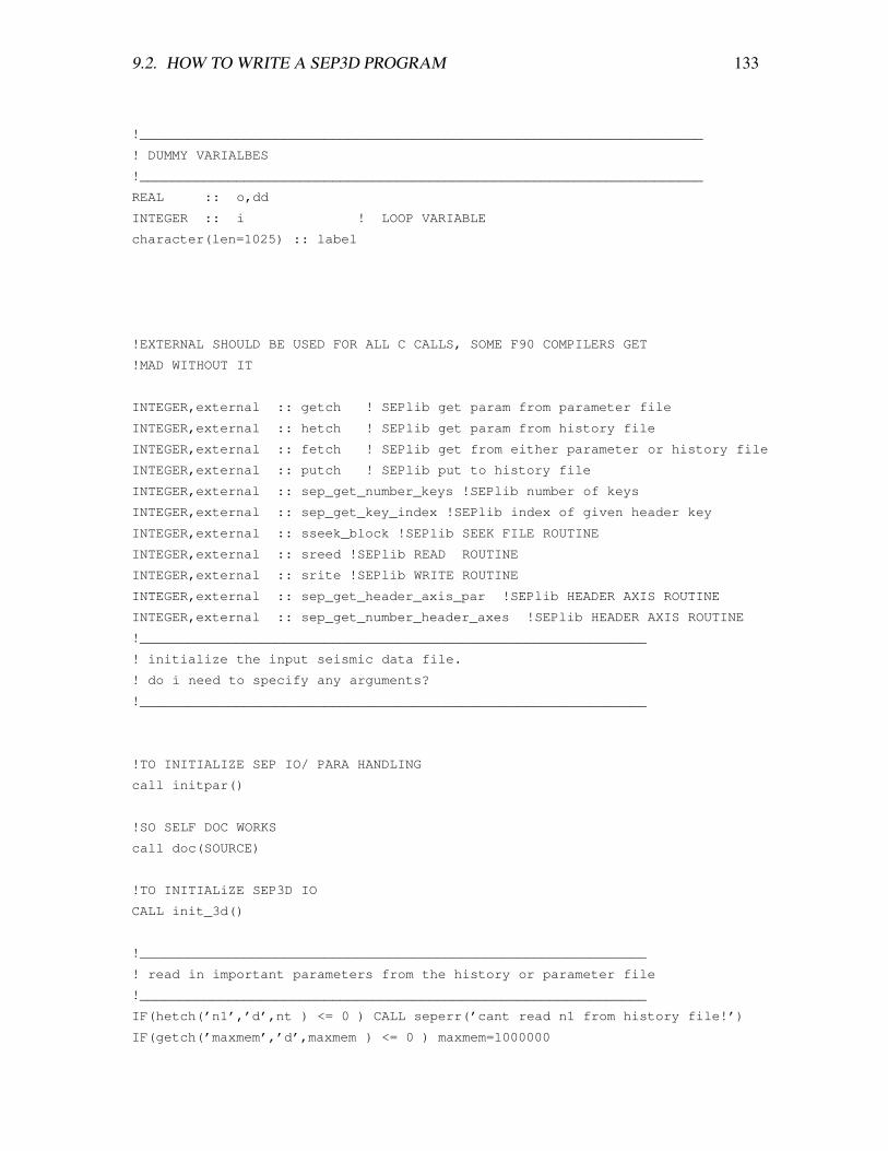
9.2. HOW TO WRITE A SEP3D PROGRAM 133
!______________________________________________________________________
! DUMMY VARIALBES
!______________________________________________________________________
REAL :: o,dd
INTEGER :: i ! LOOP VARIABLE
character(len=1025) :: label
!EXTERNAL SHOULD BE USED FOR ALL C CALLS, SOME F90 COMPILERS GET
!MAD WITHOUT IT
INTEGER,external :: getch ! SEPlib get param from parameter file
INTEGER,external :: hetch ! SEPlib get param from history file
INTEGER,external :: fetch ! SEPlib get from either parameter or history file
INTEGER,external :: putch ! SEPlib put to history file
INTEGER,external :: sep_get_number_keys !SEPlib number of keys
INTEGER,external :: sep_get_key_index !SEPlib index of given header key
INTEGER,external :: sseek_block !SEPlib SEEK FILE ROUTINE
INTEGER,external :: sreed !SEPlib READ ROUTINE
INTEGER,external :: srite !SEPlib WRITE ROUTINE
INTEGER,external :: sep_get_header_axis_par !SEPlib HEADER AXIS ROUTINE
INTEGER,external :: sep_get_number_header_axes !SEPlib HEADER AXIS ROUTINE
!_______________________________________________________________
! initialize the input seismic data file.
! do i need to specify any arguments?
!_______________________________________________________________
!TO INITIALIZE SEP IO/ PARA HANDLING
call initpar()
!SO SELF DOC WORKS
call doc(SOURCE)
!TO INITIALiZE SEP3D IO
CALL init_3d()
!_______________________________________________________________
! read in important parameters from the history or parameter file
!_______________________________________________________________
IF(hetch(’n1’,’d’,nt ) <= 0 ) CALL seperr(’cant read n1 from history file!’)
IF(getch(’maxmem’,’d’,maxmem ) <= 0 ) maxmem=1000000
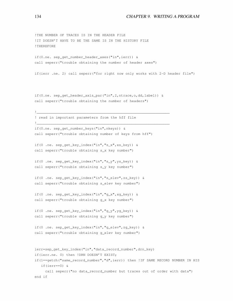
134 CHAPTER 9. WRITING A PROGRAM
!THE NUMBER OF TRACES IS IN THE HEADER FILE
!IT DOESN’T HAVE TO BE THE SAME IS IN THE HISTORY FILE
!THEREFORE
if(0.ne. sep_get_number_header_axes("in",ierr)) &
call seperr("trouble obtaining the number of header axes")
if(ierr .ne. 2) call seperr("for right now only works with 2-D header file")
if(0.ne. sep_get_header_axis_par("in",2,ntrace,o,dd,label)) &
call seperr("trouble obtaining the number of headers")
!_______________________________________________________________
! read in important parameters from the hff file
!_______________________________________________________________
if(0.ne. sep_get_number_keys("in",nkeys)) &
call seperr("trouble obtaining number of keys from hff")
if(0 .ne. sep_get_key_index("in","s_x",xs_key)) &
call seperr("trouble obtaining s_x key number")
if(0 .ne. sep_get_key_index("in","s_y",ys_key)) &
call seperr("trouble obtaining s_y key number")
if(0 .ne. sep_get_key_index("in","s_elev",zs_key)) &
call seperr("trouble obtaining s_elev key number")
if(0 .ne. sep_get_key_index("in","g_x",xg_key)) &
call seperr("trouble obtaining g_x key number")
if(0 .ne. sep_get_key_index("in","g_y",yg_key)) &
call seperr("trouble obtaining g_y key number")
if(0 .ne. sep_get_key_index("in","g_elev",zg_key)) &
call seperr("trouble obtaining g_elev key number")
ierr=sep_get_key_index("in","data_record_number",drn_key)
if(ierr.ne. 0) then !DRN DOESN’T EXIST;
if(1==getch("same_record_number","d",ierr)) then !IF SAME RECORD NUMBER IN HIS
if(ierr==0) &
call seperr("no data_record_number but traces out of order with data")
end if
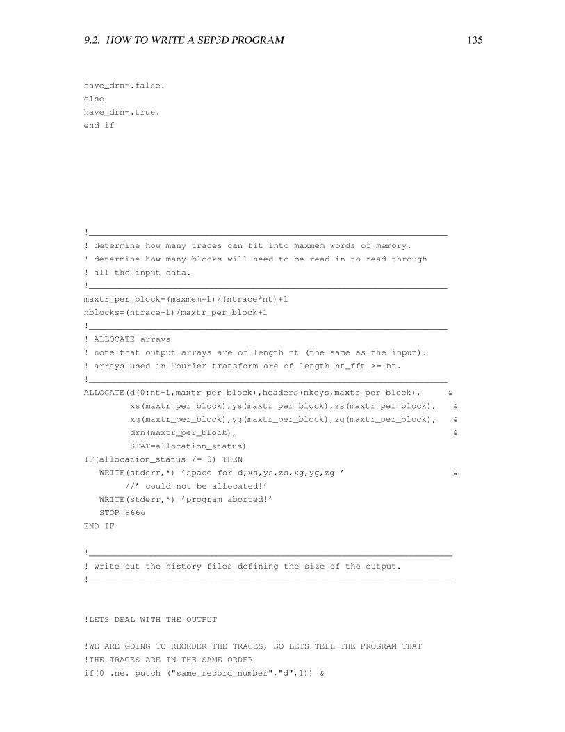
9.2. HOW TO WRITE A SEP3D PROGRAM 135
have_drn=.false.
else
have_drn=.true.
end if
!______________________________________________________________________
! determine how many traces can fit into maxmem words of memory.
! determine how many blocks will need to be read in to read through
! all the input data.
!______________________________________________________________________
maxtr_per_block=(maxmem-1)/(ntrace*nt)+1
nblocks=(ntrace-1)/maxtr_per_block+1
!______________________________________________________________________
! ALLOCATE arrays
! note that output arrays are of length nt (the same as the input).
! arrays used in Fourier transform are of length nt_fft >= nt.
!______________________________________________________________________
ALLOCATE(d(0:nt-1,maxtr_per_block),headers(nkeys,maxtr_per_block), &
xs(maxtr_per_block),ys(maxtr_per_block),zs(maxtr_per_block), &
xg(maxtr_per_block),yg(maxtr_per_block),zg(maxtr_per_block), &
drn(maxtr_per_block), &
STAT=allocation_status)
IF(allocation_status /= 0) THEN
WRITE(stderr,*) ’space for d,xs,ys,zs,xg,yg,zg ’ &
//’ could not be allocated!’
WRITE(stderr,*) ’program aborted!’
STOP 9666
END IF
!_______________________________________________________________________
! write out the history files defining the size of the output.
!_______________________________________________________________________
!LETS DEAL WITH THE OUTPUT
!WE ARE GOING TO REORDER THE TRACES, SO LETS TELL THE PROGRAM THAT
!THE TRACES ARE IN THE SAME ORDER
if(0 .ne. putch ("same_record_number","d",1)) &
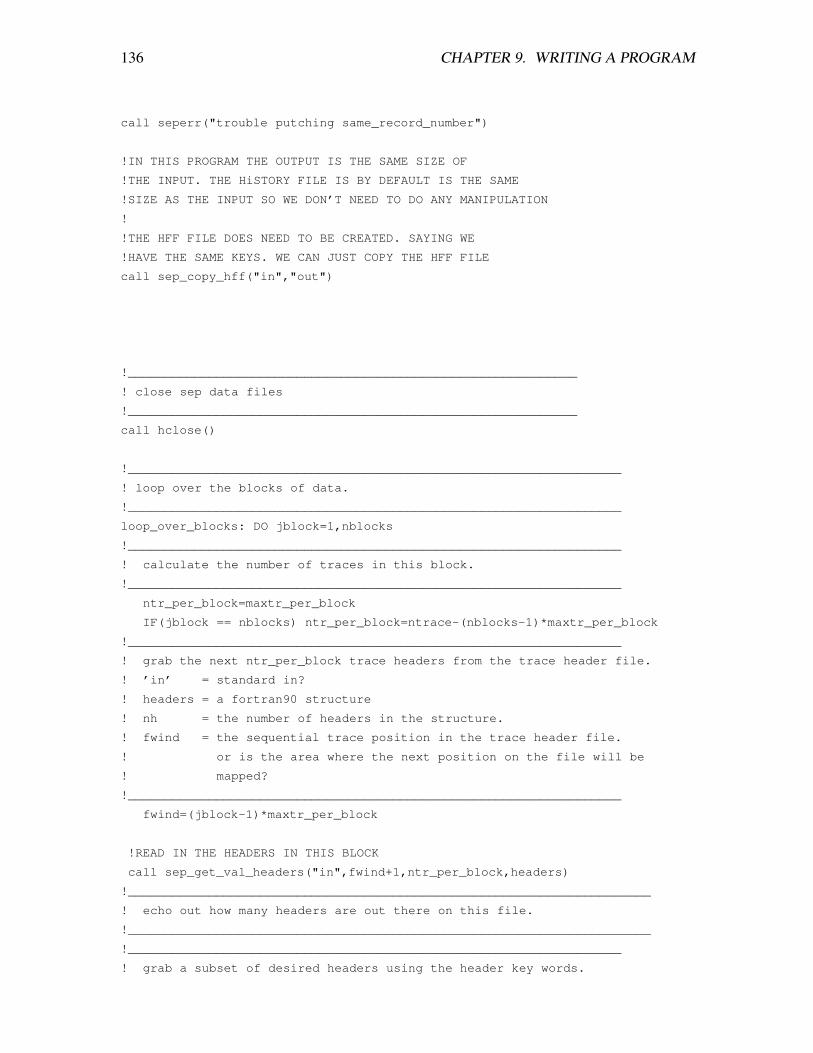
136 CHAPTER 9. WRITING A PROGRAM
call seperr("trouble putching same_record_number")
!IN THIS PROGRAM THE OUTPUT IS THE SAME SIZE OF
!THE INPUT. THE HiSTORY FILE IS BY DEFAULT IS THE SAME
!SIZE AS THE INPUT SO WE DON’T NEED TO DO ANY MANIPULATION
!
!THE HFF FILE DOES NEED TO BE CREATED. SAYING WE
!HAVE THE SAME KEYS. WE CAN JUST COPY THE HFF FILE
call sep_copy_hff("in","out")
!_____________________________________________________________
! close sep data files
!_____________________________________________________________
call hclose()
!___________________________________________________________________
! loop over the blocks of data.
!___________________________________________________________________
loop_over_blocks: DO jblock=1,nblocks
!___________________________________________________________________
! calculate the number of traces in this block.
!___________________________________________________________________
ntr_per_block=maxtr_per_block
IF(jblock == nblocks) ntr_per_block=ntrace-(nblocks-1)*maxtr_per_block
!___________________________________________________________________
! grab the next ntr_per_block trace headers from the trace header file.
! ’in’ = standard in?
! headers = a fortran90 structure
! nh = the number of headers in the structure.
! fwind = the sequential trace position in the trace header file.
! or is the area where the next position on the file will be
! mapped?
!___________________________________________________________________
fwind=(jblock-1)*maxtr_per_block
!READ IN THE HEADERS IN THIS BLOCK
call sep_get_val_headers("in",fwind+1,ntr_per_block,headers)
!_______________________________________________________________________
! echo out how many headers are out there on this file.
!_______________________________________________________________________
!___________________________________________________________________
! grab a subset of desired headers using the header key words.
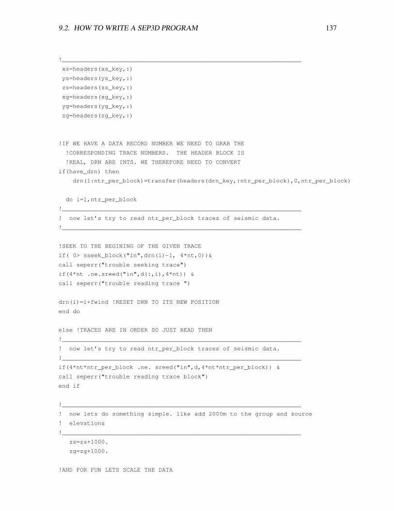
9.2. HOW TO WRITE A SEP3D PROGRAM 137
!___________________________________________________________________
xs=headers(xs_key,:)
ys=headers(ys_key,:)
zs=headers(zs_key,:)
xg=headers(xg_key,:)
yg=headers(yg_key,:)
zg=headers(zg_key,:)
!IF WE HAVE A DATA RECORD NUMBER WE NEED TO GRAB THE
!CORRESPONDING TRACE NUMBERS. THE HEADER BLOCK IS
!REAL, DRN ARE INTS. WE THEREFORE NEED TO CONVERT
if(have_drn) then
drn(1:ntr_per_block)=transfer(headers(drn_key,:ntr_per_block),0,ntr_per_block)
do i=1,ntr_per_block
!___________________________________________________________________
! now let’s try to read ntr_per_block traces of seismic data.
!___________________________________________________________________
!SEEK TO THE BEGINING OF THE GIVEN TRACE
if( 0> sseek_block("in",drn(i)-1, 4*nt,0))&
call seperr("trouble seeking trace")
if(4*nt .ne.sreed("in",d(:,i),4*nt)) &
call seperr("trouble reading trace ")
drn(i)=i+fwind !RESET DRN TO ITS NEW POSITION
end do
else !TRACES ARE IN ORDER SO JUST READ THEN
!___________________________________________________________________
! now let’s try to read ntr_per_block traces of seismic data.
!___________________________________________________________________
if(4*nt*ntr_per_block .ne. sreed("in",d,4*nt*ntr_per_block)) &
call seperr("trouble reading trace block")
end if
!___________________________________________________________________
! now lets do something simple. like add 2000m to the group and source
! elevations
!___________________________________________________________________
zs=zs+1000.
zg=zg+1000.
!AND FOR FUN LETS SCALE THE DATA
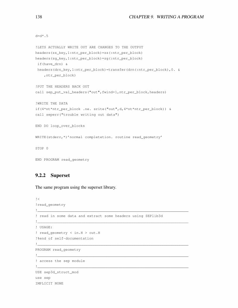
138 CHAPTER 9. WRITING A PROGRAM
d=d*.5
!LETS ACTUALLY WRITE OUT ARE CHANGES TO THE OUTPUT
headers(zs_key,1:ntr_per_block)=zs(:ntr_per_block)
headers(zg_key,1:ntr_per_block)=zg(:ntr_per_block)
if(have_drn) &
headers(drn_key,1:ntr_per_block)=transfer(drn(:ntr_per_block),0. &
,ntr_per_block)
!PUT THE HEADERS BACK OUT
call sep_put_val_headers("out",fwind+1,ntr_per_block,headers)
!WRITE THE DATA
if(4*nt*ntr_per_block .ne. srite("out",d,4*nt*ntr_per_block)) &
call seperr("trouble writing out data")
END DO loop_over_blocks
WRITE(stderr,*)’normal completetion. routine read_geometry’
STOP 0
END PROGRAM read_geometry
9.2.2 Superset
The same program using the superset library.
!<
!read_geometry
!______________________________________________________________________
! read in some data and extract some headers using SEPlib3d
!______________________________________________________________________
! USAGE:
! read_geometry < in.H > out.H
!%end of self-documentation
!______________________________________________________________________
PROGRAM read_geometry
!______________________________________________________________________
! access the sep module
!______________________________________________________________________
USE sep3d_struct_mod
use sep
IMPLICIT NONE
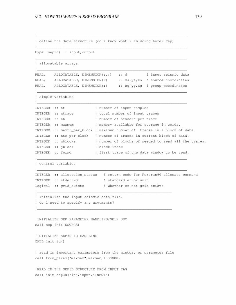
9.2. HOW TO WRITE A SEP3D PROGRAM 139
!______________________________________________________________________
! define the data structure (do i know what i am doing here? Yep)
!______________________________________________________________________
type (sep3d) :: input,output
!______________________________________________________________________
! allocatable arrays
!______________________________________________________________________
REAL, ALLOCATABLE, DIMENSION(:,:) :: d ! input seismic data
REAL, ALLOCATABLE, DIMENSION(:) :: xs,ys,zs ! source coordinates
REAL, ALLOCATABLE, DIMENSION(:) :: xg,yg,zg ! group coordinates
!______________________________________________________________________
! simple variables
!______________________________________________________________________
INTEGER :: nt ! number of input samples
INTEGER :: ntrace ! total number of input traces
INTEGER :: nh ! number of headers per trace
INTEGER :: maxmem ! memory available for storage in words.
INTEGER :: maxtr_per_block ! maximum number of traces in a block of data.
INTEGER :: ntr_per_block ! number of traces in current block of data.
INTEGER :: nblocks ! number of blocks of needed to read all the traces.
INTEGER :: jblock ! block index
INTEGER :: fwind ! first trace of the data window to be read.
!______________________________________________________________________
! control variables
!______________________________________________________________________
INTEGER :: allocation_status ! return code for Fortran90 allocate command
INTEGER :: stderr=0 ! standard error unit
logical :: grid_exists ! Whether or not grid exists
!_______________________________________________________________
! initialize the input seismic data file.
! do i need to specify any arguments?
!_______________________________________________________________
!INITIALIZE SEP PARAMETER HANDLING/SELF DOC
call sep_init(SOURCE)
!INITIALIZE SEP3D IO HANDLING
CALL init_3d()
! read in important parameters from the history or parameter file
call from_param("maxmem",maxmem,1000000)
!READ IN THE SEP3D STRUCTURE FROM INPUT TAG
call init_sep3d("in",input,"INPUT")
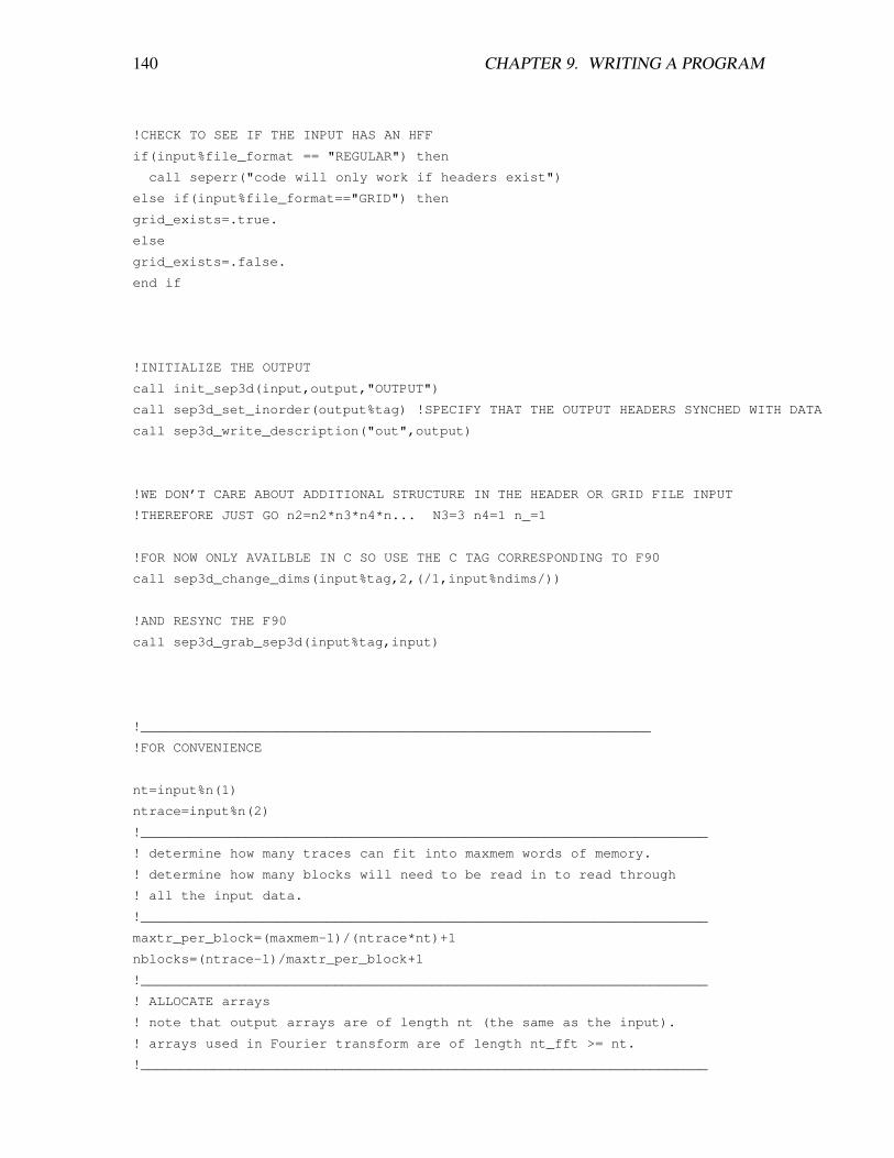
140 CHAPTER 9. WRITING A PROGRAM
!CHECK TO SEE IF THE INPUT HAS AN HFF
if(input%file_format == "REGULAR") then
call seperr("code will only work if headers exist")
else if(input%file_format=="GRID") then
grid_exists=.true.
else
grid_exists=.false.
end if
!INITIALIZE THE OUTPUT
call init_sep3d(input,output,"OUTPUT")
call sep3d_set_inorder(output%tag) !SPECIFY THAT THE OUTPUT HEADERS SYNCHED WITH DATA
call sep3d_write_description("out",output)
!WE DON’T CARE ABOUT ADDITIONAL STRUCTURE IN THE HEADER OR GRID FILE INPUT
!THEREFORE JUST GO n2=n2*n3*n4*n... N3=3 n4=1 n_=1
!FOR NOW ONLY AVAILBLE IN C SO USE THE C TAG CORRESPONDING TO F90
call sep3d_change_dims(input%tag,2,(/1,input%ndims/))
!AND RESYNC THE F90
call sep3d_grab_sep3d(input%tag,input)
!_______________________________________________________________
!FOR CONVENIENCE
nt=input%n(1)
ntrace=input%n(2)
!______________________________________________________________________
! determine how many traces can fit into maxmem words of memory.
! determine how many blocks will need to be read in to read through
! all the input data.
!______________________________________________________________________
maxtr_per_block=(maxmem-1)/(ntrace*nt)+1
nblocks=(ntrace-1)/maxtr_per_block+1
!______________________________________________________________________
! ALLOCATE arrays
! note that output arrays are of length nt (the same as the input).
! arrays used in Fourier transform are of length nt_fft >= nt.
!______________________________________________________________________
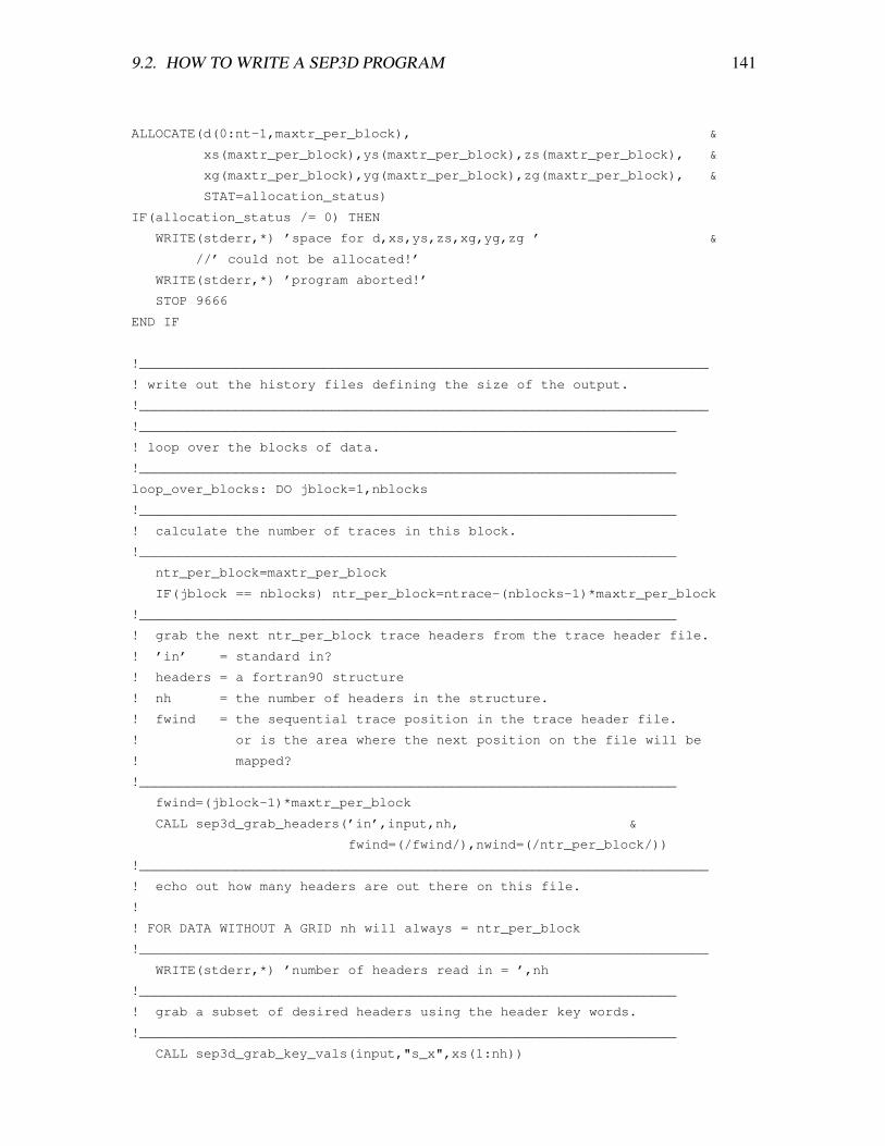
9.2. HOW TO WRITE A SEP3D PROGRAM 141
ALLOCATE(d(0:nt-1,maxtr_per_block), &
xs(maxtr_per_block),ys(maxtr_per_block),zs(maxtr_per_block), &
xg(maxtr_per_block),yg(maxtr_per_block),zg(maxtr_per_block), &
STAT=allocation_status)
IF(allocation_status /= 0) THEN
WRITE(stderr,*) ’space for d,xs,ys,zs,xg,yg,zg ’ &
//’ could not be allocated!’
WRITE(stderr,*) ’program aborted!’
STOP 9666
END IF
!_______________________________________________________________________
! write out the history files defining the size of the output.
!_______________________________________________________________________
!___________________________________________________________________
! loop over the blocks of data.
!___________________________________________________________________
loop_over_blocks: DO jblock=1,nblocks
!___________________________________________________________________
! calculate the number of traces in this block.
!___________________________________________________________________
ntr_per_block=maxtr_per_block
IF(jblock == nblocks) ntr_per_block=ntrace-(nblocks-1)*maxtr_per_block
!___________________________________________________________________
! grab the next ntr_per_block trace headers from the trace header file.
! ’in’ = standard in?
! headers = a fortran90 structure
! nh = the number of headers in the structure.
! fwind = the sequential trace position in the trace header file.
! or is the area where the next position on the file will be
! mapped?
!___________________________________________________________________
fwind=(jblock-1)*maxtr_per_block
CALL sep3d_grab_headers(’in’,input,nh, &
fwind=(/fwind/),nwind=(/ntr_per_block/))
!_______________________________________________________________________
! echo out how many headers are out there on this file.
!
! FOR DATA WITHOUT A GRID nh will always = ntr_per_block
!_______________________________________________________________________
WRITE(stderr,*) ’number of headers read in = ’,nh
!___________________________________________________________________
! grab a subset of desired headers using the header key words.
!___________________________________________________________________
CALL sep3d_grab_key_vals(input,"s_x",xs(1:nh))
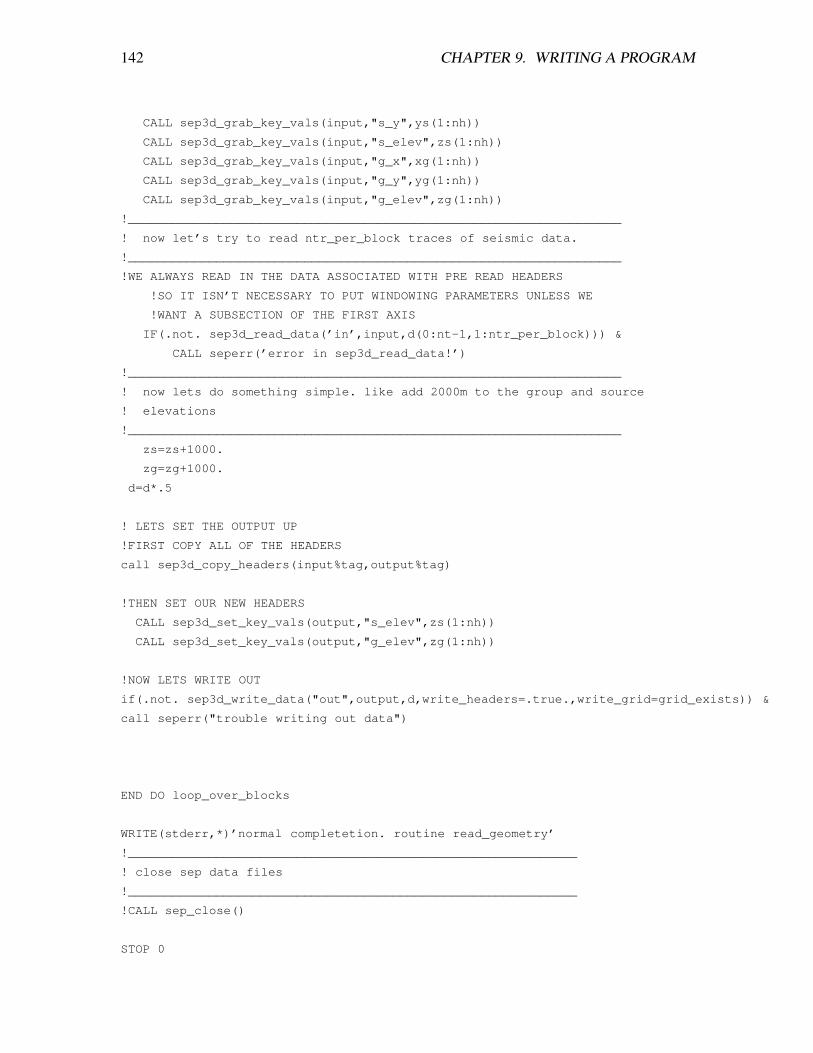
142 CHAPTER 9. WRITING A PROGRAM
CALL sep3d_grab_key_vals(input,"s_y",ys(1:nh))
CALL sep3d_grab_key_vals(input,"s_elev",zs(1:nh))
CALL sep3d_grab_key_vals(input,"g_x",xg(1:nh))
CALL sep3d_grab_key_vals(input,"g_y",yg(1:nh))
CALL sep3d_grab_key_vals(input,"g_elev",zg(1:nh))
!___________________________________________________________________
! now let’s try to read ntr_per_block traces of seismic data.
!___________________________________________________________________
!WE ALWAYS READ IN THE DATA ASSOCIATED WITH PRE READ HEADERS
!SO IT ISN’T NECESSARY TO PUT WINDOWING PARAMETERS UNLESS WE
!WANT A SUBSECTION OF THE FIRST AXIS
IF(.not. sep3d_read_data(’in’,input,d(0:nt-1,1:ntr_per_block))) &
CALL seperr(’error in sep3d_read_data!’)
!___________________________________________________________________
! now lets do something simple. like add 2000m to the group and source
! elevations
!___________________________________________________________________
zs=zs+1000.
zg=zg+1000.
d=d*.5
! LETS SET THE OUTPUT UP
!FIRST COPY ALL OF THE HEADERS
call sep3d_copy_headers(input%tag,output%tag)
!THEN SET OUR NEW HEADERS
CALL sep3d_set_key_vals(output,"s_elev",zs(1:nh))
CALL sep3d_set_key_vals(output,"g_elev",zg(1:nh))
!NOW LETS WRITE OUT
if(.not. sep3d_write_data("out",output,d,write_headers=.true.,write_grid=grid_exists)) &
call seperr("trouble writing out data")
END DO loop_over_blocks
WRITE(stderr,*)’normal completetion. routine read_geometry’
!_____________________________________________________________
! close sep data files
!_____________________________________________________________
!CALL sep_close()
STOP 0
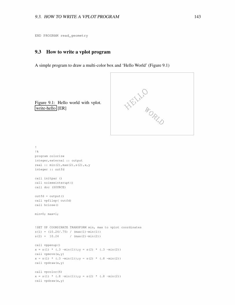
9.3. HOW TO WRITE A VPLOT PROGRAM 143
END PROGRAM read_geometry
9.3 How to write a vplot program
A simple program to draw a multi-color box and ‘Hello World’ (Figure 9.1)
Figure 9.1: Hello world with vplot.write-hello [ER]
!
!%
program colorize
integer,external :: output
real :: min(2),max(2),s(2),x,y
integer :: outfd
call initpar ()
call noieeeinterupt()
call doc (SOURCE)
outfd = output()
call vpfilep( outfd)
call hclose()
min=0; max=1;
!SET UP COORDINATE TRANSFORM min, max to vplot coordinates
s(1) = (10.24/.75) / (max(1)-min(1))
s(2) = 10.24 / (max(2)-min(2))
call vppenup()
x = s(1) * (.3 -min(1));y = s(2) * (.3 -min(2))
call vpmove(x,y)
x = s(1) * (.3 -min(1));y = s(2) * (.8 -min(2))
call vpdraw(x,y)
call vpcolor(6)
x = s(1) * (.8 -min(1));y = s(2) * (.8 -min(2))
call vpdraw(x,y)
144 CHAPTER 9. WRITING A PROGRAM
call vpcolor(5)
x = s(1) * (.8 -min(1));y = s(2) * (.3 -min(2))
call vpdraw(x,y)
call vpcolor(4)
x = s(1) * (.3 -min(1));y = s(2) * (.3 -min(2))
call vpdraw(x,y)
call vpcolor(3)
x = s(1) * (.4 -min(1));y = s(2) * (.5 -min(2))
call vptext(x,y,15,40,"HELLO")
call vpcolor(2)
x = s(1) * (.5 -min(1));y = s(2) * (.5 -min(2))
call vptext(x,y,12,-40,"WORLD")
call vppenup()
end program
9.4 Writing in SEP’s Fortran90 inversion library
9.4.1 Out-of-core
Geophysical processing is often complicated by the large datasets, particularly when dealingwith 3-D data. A solution for the large size problems is to implement inversion in an out-of-core fashion, where only limited chunks of the model and data are kept in memory at anygiven time. This is the purpose of the oclib optimization library introduced in the Librarieschapter and further explained here.
Generally speaking, the types of problems that can be solved using this library are regu-larized inversion in standard form
[
WL
εA
]
m≈[
WD0
]
, (9.1)
or in its preconditioned form[
WLP
ε I
]
p≈[
WD0
]
, (9.2)
where A is a regularization operator, W is a weighting operator, P is a preconditioning oper-ator, and p is the preconditioned form of m.
The operators L, A, W , P are application-dependent and therefore have to be externallyimplemented, likely in an out-of-core manner, by the user of the library. All other operationsneeded to solve the inversion problem are build into oclib.
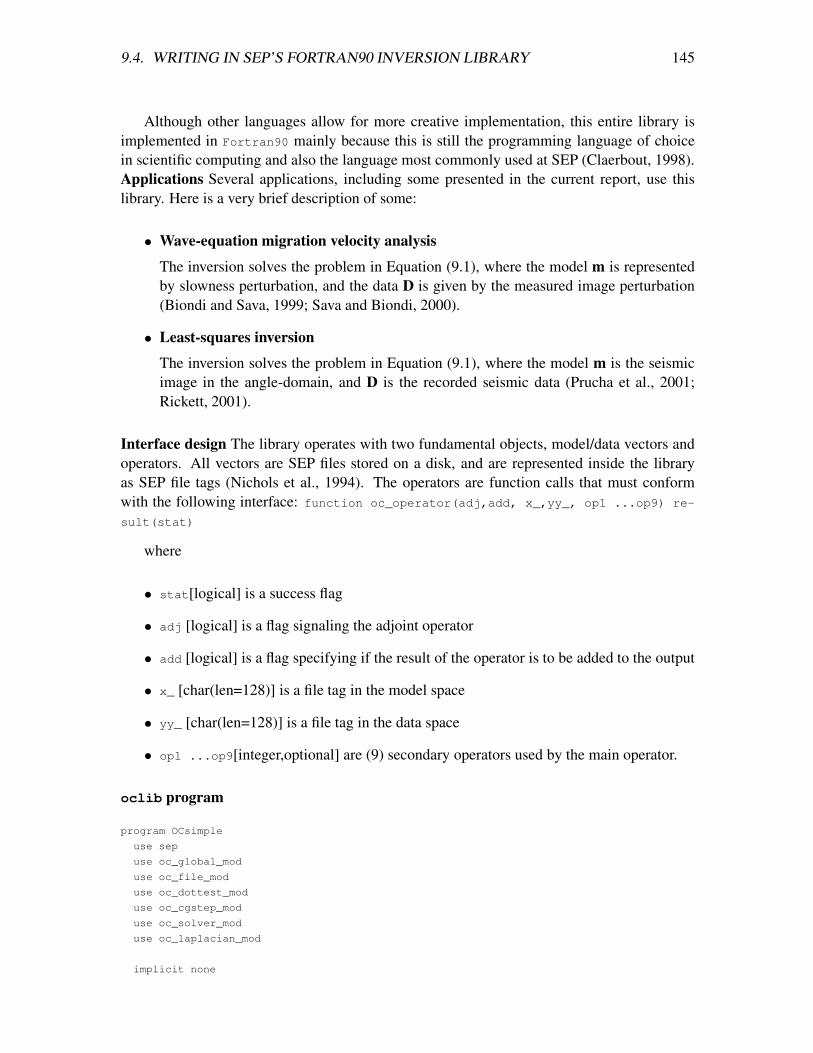
9.4. WRITING IN SEP’S FORTRAN90 INVERSION LIBRARY 145
Although other languages allow for more creative implementation, this entire library isimplemented in Fortran90 mainly because this is still the programming language of choicein scientific computing and also the language most commonly used at SEP (Claerbout, 1998).Applications Several applications, including some presented in the current report, use thislibrary. Here is a very brief description of some:
• Wave-equation migration velocity analysis
The inversion solves the problem in Equation (9.1), where the model m is representedby slowness perturbation, and the data D is given by the measured image perturbation(Biondi and Sava, 1999; Sava and Biondi, 2000).
• Least-squares inversion
The inversion solves the problem in Equation (9.1), where the model m is the seismicimage in the angle-domain, and D is the recorded seismic data (Prucha et al., 2001;Rickett, 2001).
Interface design The library operates with two fundamental objects, model/data vectors andoperators. All vectors are SEP files stored on a disk, and are represented inside the libraryas SEP file tags (Nichols et al., 1994). The operators are function calls that must conformwith the following interface: function oc_operator(adj,add, x_,yy_, op1 ...op9) re-
sult(stat)
where
• stat[logical] is a success flag
• adj [logical] is a flag signaling the adjoint operator
• add [logical] is a flag specifying if the result of the operator is to be added to the output
• x_ [char(len=128)] is a file tag in the model space
• yy_ [char(len=128)] is a file tag in the data space
• op1 ...op9[integer,optional] are (9) secondary operators used by the main operator.
oclib program
program OCsimple
use sep
use oc_global_mod
use oc_file_mod
use oc_dottest_mod
use oc_cgstep_mod
use oc_solver_mod
use oc_laplacian_mod
implicit none
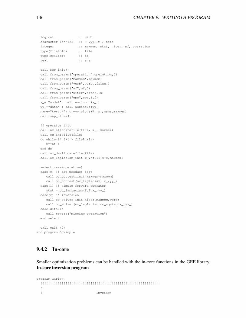
146 CHAPTER 9. WRITING A PROGRAM
logical :: verb
character(len=128) :: x_,yy_,t_, name
integer :: maxmem, stat, niter, nf, operation
type(fileinfo) :: file
type(cfilter) :: aa
real :: eps
call sep_init()
call from_param("operation",operation,0)
call from_param("maxmem",maxmem)
call from_param("verb",verb,.false.)
call from_param("nf",nf,5)
call from_param("niter",niter,10)
call from_param("eps",eps,1.0)
x_= "model"; call auxinout(x_ )
yy_="data" ; call auxinout(yy_)
name="test.H"; t_=oc_clone(F, x_,name,maxmem)
call sep_close()
!! operator init
call oc_allocatefile(file, x_, maxmem)
call oc_infofile(file)
do while(2*nf+1 > file%n(1))
nf=nf-1
end do
call oc_deallocatefile(file)
call oc_laplacian_init(x_,nf,10,0.0,maxmem)
select case(operation)
case(0) !! dot product test
call oc_dottest_init(maxmem=maxmem)
call oc_dottest(oc_laplacian, x_,yy_)
case(1) !! simple forward operator
stat = oc_laplacian(F,F,x_,yy_)
case(2) !! inversion
call oc_solver_init(niter,maxmem,verb)
call oc_solver(oc_laplacian,oc_cgstep,x_,yy_)
case default
call seperr("missing operation")
end select
call exit (0)
end program OCsimple
9.4.2 In-core
Smaller optimization problems can be handled with the in-core functions in the GEE library.In-core inversion program
program Carlos
!!!!!!!!!!!!!!!!!!!!!!!!!!!!!!!!!!!!!!!!!!!!!!!!!!!!!!!!!!!!!!
!
! Invstack
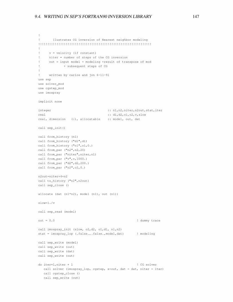
9.4. WRITING IN SEP’S FORTRAN90 INVERSION LIBRARY 147
!
! Ilustrates CG inversion of Nearest neighbor modeling
!!!!!!!!!!!!!!!!!!!!!!!!!!!!!!!!!!!!!!!!!!!!!!!!!!!!!!!!!!!!!!
!
! v = velocity (if constant)
! niter = number of steps of the CG inversion
! out = input model + modeling +result of transpose of mod
! + subsequent steps of CG
!
! written by carlos and jon 6-11-91
use sep
use solver_mod
use cgstep_mod
use imospray
implicit none
integer :: n1,n2,niter,n2out,stat,iter
real :: d1,d2,o1,o2,v,slow
real, dimension (:), allocatable :: model, out, dat
call sep_init()
call from_history (n1)
call from_history ("d1",d1)
call from_history ("o1",o1,0.)
call from_par ("n2",n2,20)
call from_par ("niter",niter,n1)
call from_par ("v",v,1000.)
call from_par ("d2",d2,200.)
call from_par ("o2",o2,0.)
n2out=niter+4+n2
call to_history ("n2",n2out)
call sep_close ()
allocate (dat (n1*n2), model (n1), out (n1))
slow=1./v
call sep_read (model)
out = 0.0 ! dummy trace
call imospray_init (slow, o2,d2, o1,d1, n1,n2)
stat = imospray_lop (.false.,.false.,model,dat) ! modeling
call sep_write (model)
call sep_write (out)
call sep_write (dat)
call sep_write (out)
do iter=1,niter + 1 ! CG solver
call solver (imospray_lop, cgstep, x=out, dat = dat, niter = iter)
call cgstep_close ()
call sep_write (out)
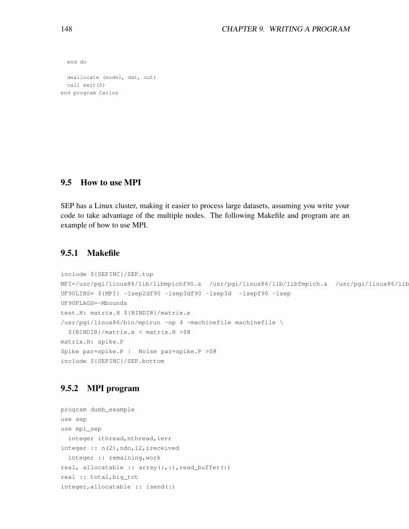
148 CHAPTER 9. WRITING A PROGRAM
end do
deallocate (model, dat, out)
call exit(0)
end program Carlos
9.5 How to use MPI
SEP has a Linux cluster, making it easier to process large datasets, assuming you write yourcode to take advantage of the multiple nodes. The following Makefile and program are anexample of how to use MPI.
9.5.1 Makefile
include ${SEPINC}/SEP.top
MPI=/usr/pgi/linux86/lib/libmpichf90.a /usr/pgi/linux86/lib/libfmpich.a /usr/pgi/linux86/lib/libmpich.a
UF90LIBS= ${MPI} -lsep2df90 -lsep3df90 -lsep3d -lsepf90 -lsep
UF90FLAGS=-Mbounds
test.H: matrix.H ${BINDIR}/matrix.x
/usr/pgi/linux86/bin/mpirun -np 4 -machinefile machinefile \
${BINDIR}/matrix.x < matrix.H >$@
matrix.H: spike.P
Spike par=spike.P | Noise par=spike.P >$@
include ${SEPINC}/SEP.bottom
9.5.2 MPI program
program dumb_example
use sep
use mpi_sep
integer ithread,nthread,ierr
integer :: n(2),ndo,i2,ireceived
integer :: remaining,work
real, allocatable :: array(:,:),read_buffer(:)
real :: total,big_tot
integer,allocatable :: isend(:)
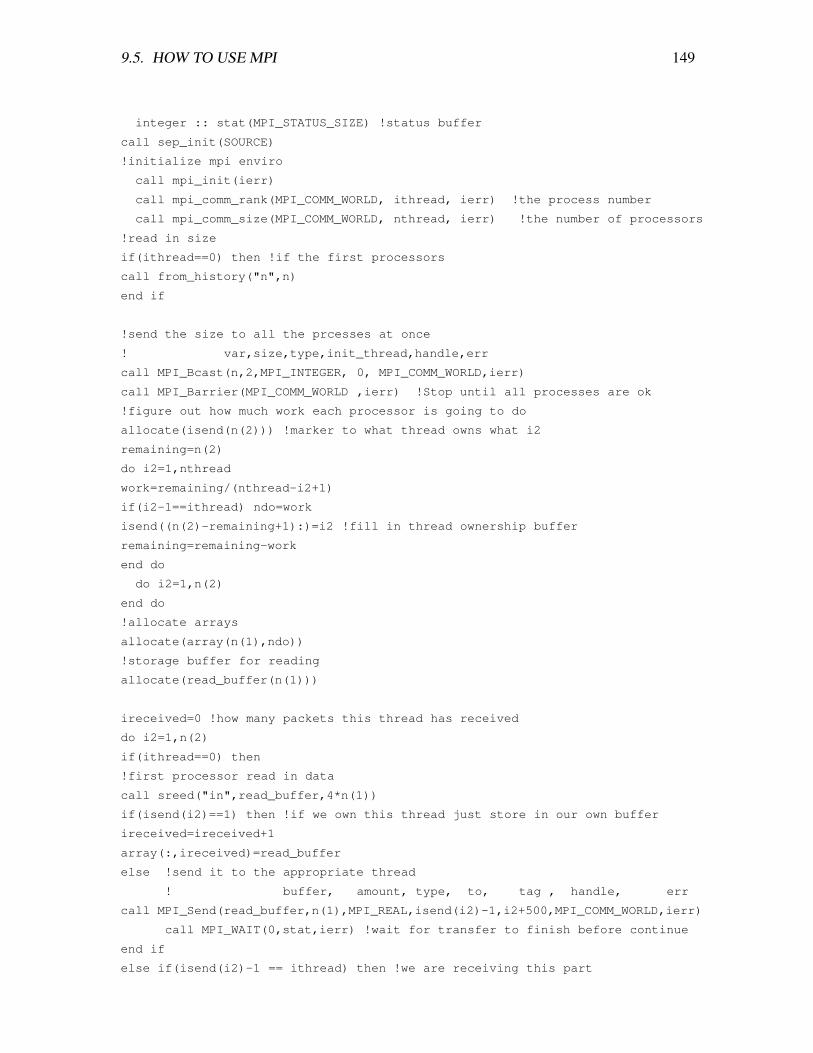
9.5. HOW TO USE MPI 149
integer :: stat(MPI_STATUS_SIZE) !status buffer
call sep_init(SOURCE)
!initialize mpi enviro
call mpi_init(ierr)
call mpi_comm_rank(MPI_COMM_WORLD, ithread, ierr) !the process number
call mpi_comm_size(MPI_COMM_WORLD, nthread, ierr) !the number of processors
!read in size
if(ithread==0) then !if the first processors
call from_history("n",n)
end if
!send the size to all the prcesses at once
! var,size,type,init_thread,handle,err
call MPI_Bcast(n,2,MPI_INTEGER, 0, MPI_COMM_WORLD,ierr)
call MPI_Barrier(MPI_COMM_WORLD ,ierr) !Stop until all processes are ok
!figure out how much work each processor is going to do
allocate(isend(n(2))) !marker to what thread owns what i2
remaining=n(2)
do i2=1,nthread
work=remaining/(nthread-i2+1)
if(i2-1==ithread) ndo=work
isend((n(2)-remaining+1):)=i2 !fill in thread ownership buffer
remaining=remaining-work
end do
do i2=1,n(2)
end do
!allocate arrays
allocate(array(n(1),ndo))
!storage buffer for reading
allocate(read_buffer(n(1)))
ireceived=0 !how many packets this thread has received
do i2=1,n(2)
if(ithread==0) then
!first processor read in data
call sreed("in",read_buffer,4*n(1))
if(isend(i2)==1) then !if we own this thread just store in our own buffer
ireceived=ireceived+1
array(:,ireceived)=read_buffer
else !send it to the appropriate thread
! buffer, amount, type, to, tag , handle, err
call MPI_Send(read_buffer,n(1),MPI_REAL,isend(i2)-1,i2+500,MPI_COMM_WORLD,ierr)
call MPI_WAIT(0,stat,ierr) !wait for transfer to finish before continue
end if
else if(isend(i2)-1 == ithread) then !we are receiving this part
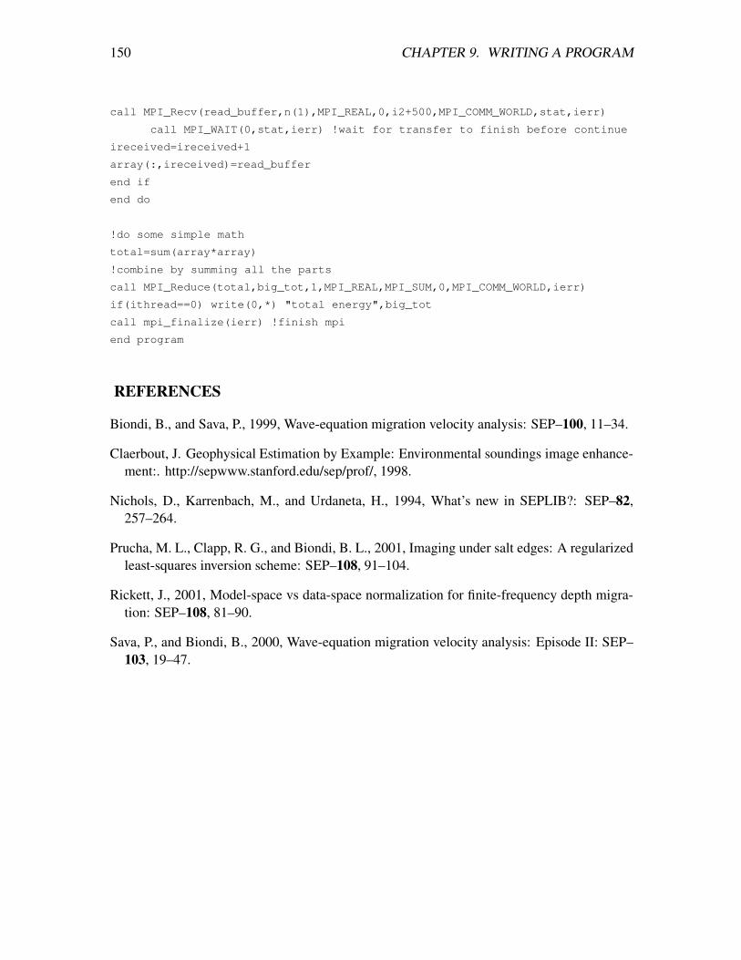
150 CHAPTER 9. WRITING A PROGRAM
call MPI_Recv(read_buffer,n(1),MPI_REAL,0,i2+500,MPI_COMM_WORLD,stat,ierr)
call MPI_WAIT(0,stat,ierr) !wait for transfer to finish before continue
ireceived=ireceived+1
array(:,ireceived)=read_buffer
end if
end do
!do some simple math
total=sum(array*array)
!combine by summing all the parts
call MPI_Reduce(total,big_tot,1,MPI_REAL,MPI_SUM,0,MPI_COMM_WORLD,ierr)
if(ithread==0) write(0,*) "total energy",big_tot
call mpi_finalize(ierr) !finish mpi
end program
REFERENCES
Biondi, B., and Sava, P., 1999, Wave-equation migration velocity analysis: SEP–100, 11–34.
Claerbout, J. Geophysical Estimation by Example: Environmental soundings image enhance-ment:. http://sepwww.stanford.edu/sep/prof/, 1998.
Nichols, D., Karrenbach, M., and Urdaneta, H., 1994, What’s new in SEPLIB?: SEP–82,257–264.
Prucha, M. L., Clapp, R. G., and Biondi, B. L., 2001, Imaging under salt edges: A regularizedleast-squares inversion scheme: SEP–108, 91–104.
Rickett, J., 2001, Model-space vs data-space normalization for finite-frequency depth migra-tion: SEP–108, 81–90.
Sava, P., and Biondi, B., 2000, Wave-equation migration velocity analysis: Episode II: SEP–103, 19–47.
Chapter 10
Preprocessors
10.1 Introduction
Fortran is generally accepted as the most universal computer language for computationalphysics. However, for general programming, it has been surpassed by C. Ratfor is Fortran withC-like syntax. Ratfor was invented by the Kernighan and Plauger(1976), the same people whoinvented C. Ratfor uses C-like syntax, the syntax that is also found in the popular languagesC++, Perl, and Java. Ratfor source is approximately 25-30% smaller than the equivalent For-tran source, so it is equivalently more readable.
Recently SEP has been shifting to the newest version of Fortran, Fortran90 (Clapp andCrawley, 1996; Fomel and Claerbout, 1996). Fortran90 allows for dynamic memory alloca-tion and adds useful programming features such as structures, but still forces a verbose codingstyle. To take advantage of Fortran90’s new features, while maintaining the concise cod-ing style provided by Ratfor, we wrote a new Ratfor preprocessor, Ratfor90, which producesFortran90 rather than Fortran77 code. The newest Ratfor “compiler”, Ratfor90, is a sim-ple word-processing program (written in Perl and freely distributed1) that inputs an attractiveFortran-like dialect and outputs Fortran90.
10.2 Ratfor basics
You should be able to read Ratfor if you already know Fortran, C, or any similar computerlanguage. The Ratfor processor is not a compiler but a simple word-processing program thatconverts the Ratfor dialect to Fortran. To maximize your use of Ratfor, you will need to knowits rules:
1http://sepwww.stanford.edu/src/ratfor90.html
151
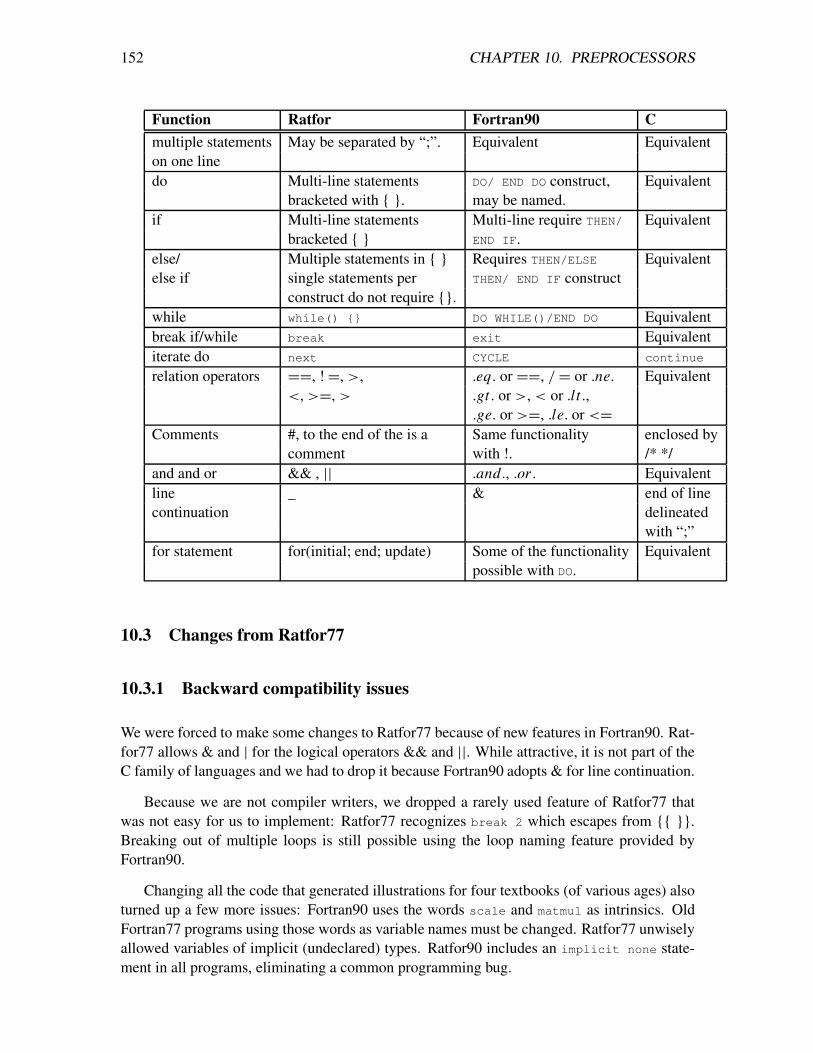
152 CHAPTER 10. PREPROCESSORS
Function Ratfor Fortran90 Cmultiple statements May be separated by “;”. Equivalent Equivalenton one linedo Multi-line statements DO/ END DO construct, Equivalent
bracketed with { }. may be named.if Multi-line statements Multi-line require THEN/ Equivalent
bracketed { } END IF.else/ Multiple statements in { } Requires THEN/ELSE Equivalentelse if single statements per THEN/ END IF construct
construct do not require {}.while while() {} DO WHILE()/END DO Equivalentbreak if/while break exit Equivalentiterate do next CYCLE continue
relation operators ==, !=, >, .eq. or ==, /= or .ne. Equivalent<, >=, > .gt . or >, < or .lt .,
.ge. or >=, .le. or <=Comments #, to the end of the is a Same functionality enclosed by
comment with !. /* */and and or && , || .and., .or . Equivalentline _ & end of linecontinuation delineated
with “;”for statement for(initial; end; update) Some of the functionality Equivalent
possible with DO.
10.3 Changes from Ratfor77
10.3.1 Backward compatibility issues
We were forced to make some changes to Ratfor77 because of new features in Fortran90. Rat-for77 allows & and | for the logical operators && and ||. While attractive, it is not part of theC family of languages and we had to drop it because Fortran90 adopts & for line continuation.
Because we are not compiler writers, we dropped a rarely used feature of Ratfor77 thatwas not easy for us to implement: Ratfor77 recognizes break 2 which escapes from {{ }}.Breaking out of multiple loops is still possible using the loop naming feature provided byFortran90.
Changing all the code that generated illustrations for four textbooks (of various ages) alsoturned up a few more issues: Fortran90 uses the words scale and matmul as intrinsics. OldFortran77 programs using those words as variable names must be changed. Ratfor77 unwiselyallowed variables of implicit (undeclared) types. Ratfor90 includes an implicit none state-ment in all programs, eliminating a common programming bug.
10.4. SEP EXTENSIONS 153
10.3.2 Extensions
New features in Ratfor90 are bracketed type, subroutine, function, where, and module state-ments. In some ways this a further step towards the C, C++, Java model. It makes complicatedmodules, subroutines inside subroutines, and other advanced features of Fortran90 easier tointerpret. Ratfor90 has better error messages than Ratfor77. Besides the use of stderr, a newfile (ratfor_problem) indicates where problems with interpreting programs are encountered.
In many geophysical applications we perform operations of the form:
c(i1,i2) = c(i1,i2) + scale * e(i1,i3,i4)
Because this type type of operation is so common we borrowed from C the += and -= operators,which changes the above line into:
c(i1,i2) += scale * e(i1,i3,i4)
10.4 SEP extensions
The large amount of code written in Ratfor77 and SEP’s saw and sat pre-processors requiredthat Ratfor90 handle the conventions that they introduced. By including the flag -sep onthe command line Ratfor90 simulates the functions of saw and sat (memory allocation andparameter handling.)
10.4.1 Memory allocation
The main method at SEP for dynamic memory allocation under Ratfor77, saw, and sat wasthe allocate statement:
allocate: real x(n1,n2)
When Ratfor90 finds this statement, along with the corresponding main program/subroutinestructure of saw and sat, it translates the allocate: statement into a Fortran allocatable
array, allocates the array, and passes it, along with all other relevant variables to the subroutine.
In subroutines SEP allowed dynamic memory allocation through the use of the temporary
keyword, for example:
temporary real*4 data(n1,n2,n3), convolution(j+k-1)
Automatic arrays are supported in Fortran90 so Ratfor90 simply translates this statement to:
real*4 data(n1,n2,n3), convolution(j+k-1).
154 CHAPTER 10. PREPROCESSORS
10.4.2 Parameter handling
In addition, saw and sat, and now Ratfor90, simplify parameter handling. Ratfor90 calls anessential SEPlib initialization routine initpar(), organizes the self-doc, and allows for vari-ous parameter handling keywords (from history, from par, from either, from aux, to
aux, to history). For example, the line:
from either: integer n1,n2:ns,n3:nv=1
is translated into the much more verbose:
if (0==fetch(’n1’,’d’,n1)) then
call seperr(’Could not obtain n1 from either’)
end if
if (0/=putch(’From either: n1’,’d’,n1)) then
call seperr(’trouble writing n1 to history file’)
end if
if (0==fetch(’n2’,’d’,ns)) then
call seperr(’Could not obtain n2 from either’)
end if
if (0/=putch(’From either: n2’,’d’,ns)) then
call seperr(’trouble writing n2 to history file’)
end if
if (0==fetch(’n3’,’d’,nv)) then
nv=1
end if
if (0/=putch(’From either: n3’,’d’,nv)) then
call seperr(’trouble writing n3 to history file’)
end if
10.4. SEP EXTENSIONS 155
As an illustration, here is a simple program to convert from interval to RMS velocities inRatfor90 and the corresponding Fortran90 code.
10.4.3 Ratfor90 code
#<
#dix
#
#Usage:
#dix <in.H >out.H
#
#Description
# Converts from interval to RMS velocity
#>
#%end of self-documentation
program dix{
integer i1,i2,i3,n1,n2,n3
real,allocatable,dimension(:,:) :: array
real time,val,dt,dx
from history: integer n1,n2,n3 #grab the size of the dataset
#from the history file
from history: real d1:dx #get the sampling interval, store in dx
allocate(array(n1,n2))
do i3=1,n3{
call sreed("in",array,n1*n2*4)
array=1./array #Fortran90 array manipulation
do i2=1,n2{
time=0.;val=0.
do i1=1,n1{
dt=dx/array(i1,i2)
val+=dt*array(i1,i2)**2 #add sum Ratfor90 feature
time+=dt
array(i1,i2)=sqrt(val/time)
}
}
call srite("out",array,n1*n2*4)
}
} #bracketed programs
10.4.4 Translated Fortran90 Code
!<
!dix
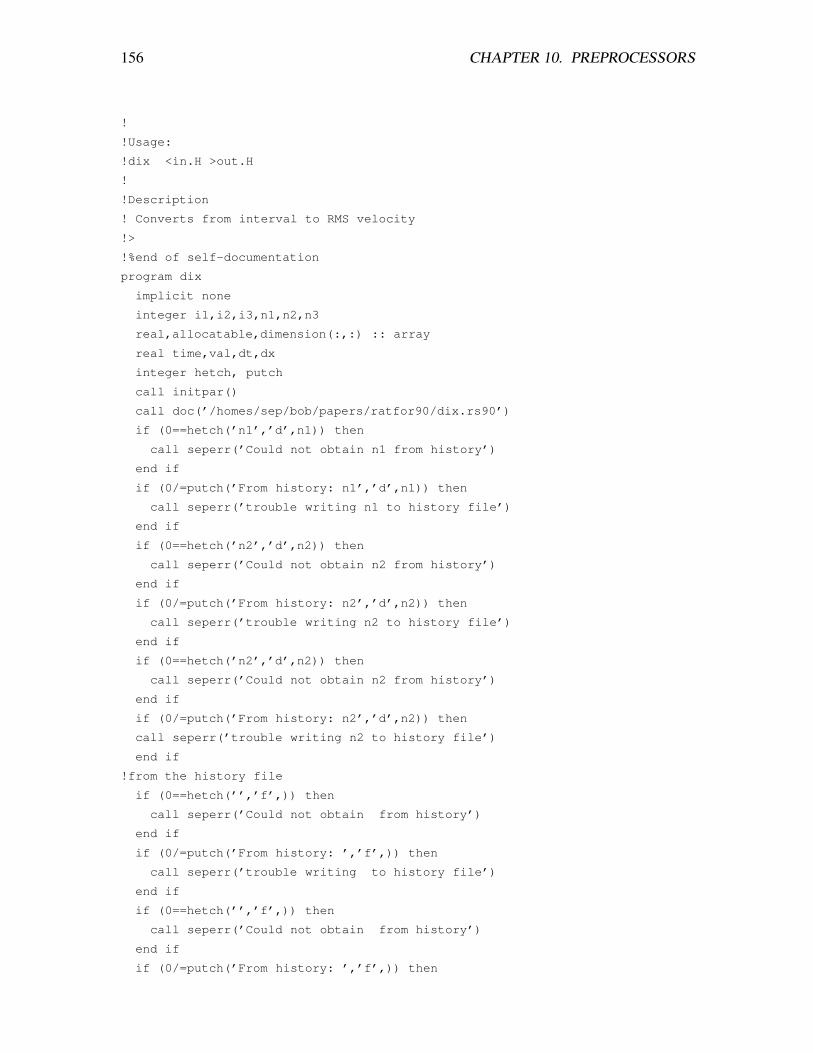
156 CHAPTER 10. PREPROCESSORS
!
!Usage:
!dix <in.H >out.H
!
!Description
! Converts from interval to RMS velocity
!>
!%end of self-documentation
program dix
implicit none
integer i1,i2,i3,n1,n2,n3
real,allocatable,dimension(:,:) :: array
real time,val,dt,dx
integer hetch, putch
call initpar()
call doc(’/homes/sep/bob/papers/ratfor90/dix.rs90’)
if (0==hetch(’n1’,’d’,n1)) then
call seperr(’Could not obtain n1 from history’)
end if
if (0/=putch(’From history: n1’,’d’,n1)) then
call seperr(’trouble writing n1 to history file’)
end if
if (0==hetch(’n2’,’d’,n2)) then
call seperr(’Could not obtain n2 from history’)
end if
if (0/=putch(’From history: n2’,’d’,n2)) then
call seperr(’trouble writing n2 to history file’)
end if
if (0==hetch(’n2’,’d’,n2)) then
call seperr(’Could not obtain n2 from history’)
end if
if (0/=putch(’From history: n2’,’d’,n2)) then
call seperr(’trouble writing n2 to history file’)
end if
!from the history file
if (0==hetch(’’,’f’,)) then
call seperr(’Could not obtain from history’)
end if
if (0/=putch(’From history: ’,’f’,)) then
call seperr(’trouble writing to history file’)
end if
if (0==hetch(’’,’f’,)) then
call seperr(’Could not obtain from history’)
end if
if (0/=putch(’From history: ’,’f’,)) then
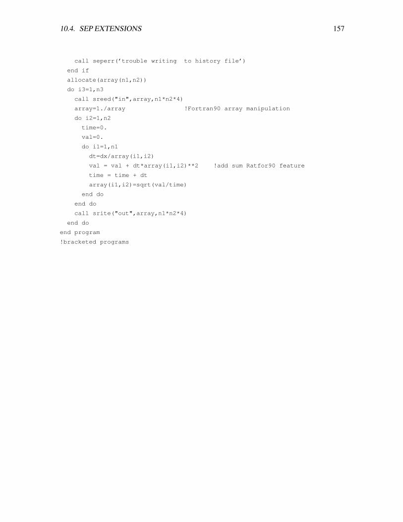
10.4. SEP EXTENSIONS 157
call seperr(’trouble writing to history file’)
end if
allocate(array(n1,n2))
do i3=1,n3
call sreed("in",array,n1*n2*4)
array=1./array !Fortran90 array manipulation
do i2=1,n2
time=0.
val=0.
do i1=1,n1
dt=dx/array(i1,i2)
val = val + dt*array(i1,i2)**2 !add sum Ratfor90 feature
time = time + dt
array(i1,i2)=sqrt(val/time)
end do
end do
call srite("out",array,n1*n2*4)
end do
end program
!bracketed programs
158 CHAPTER 10. PREPROCESSORS
10.5 Downloading/installing
You can download Ratfor90 from http://sepwww.stanford.edu/sep/bob/ratfor90/ratfor90. Youmight need to change the first line of the code indicating where perl is on your system. Youcan convert from Ratfor90 to Fortran90 on the command line by:
ratfor90 < input.r90 > output.f90
If you wish to use expanded SEP command line, history file manipulation, and self-documentationabilities add the -sep -SOURCE /my/source/location flags. An alternate approach is to usethe SEP makefile rules which are explained in Reproducible electronic documents2. If youfollow this approach you will need to:
• install ratfor90 in /usr/local/bin/ratfor90 or edit the Prg.defs.top file.
• set the environmental variable RATF90 to yes ( setenv RATF90 yes). If you are usingthe SEP setup you can add this line to your Setup/cshrc.machinetype [e.g. cshrc.sgi,cshrc.i586, etc.]
• name your Ratfor90 files:
– using Fortran90 syntax .r90.
– using Fortran90 and SEP allocation conventions .rs90.
By setting the environmental variable RATF90, SEP style ratfor77 code, normally indicated bythe .rt, .rs, and .rst suffixes will converted to Fortran90 by Ratfor90 and compiled. Theserules are in the updated version of the SEP makefile rules so if you have a previous versionyou will need to download a new one.
2http://sepwww.stanford.edu/redoc
10.6. ERROR HANDLING 159
10.6 Error handling
Ratfor90 creates a file called ratfor_problem whenever it encounters and error in the sourcecode. The ratfor_problem file contains the processed source code, with the line that causedthe processor problems clearly delineated. For example if you misspelled if in a source file:
iff(a .eq. b){
and ran the Ratfor90 processor you would see:
ERROR:
Problem finding acceptable bracket statement
I was looking for do, module,subroutine, etc before a {
and couldn’t find it (spelling?????)
wrote file as far as I got to ratfor_problem
written to stderr and in the file ratfor_problem
ERROR BEFORE ERROR
iff(a .eq. b){
ERROR AFTER
the location of the error is clearly indicated. The next time ratfor90 is run, the ratfor_problemfile is removed.
REFERENCES
Clapp, R. G., and Crawley, S., 1996, SEPF90: SEP–93, 293–304.
Fomel, S., and Claerbout, J., 1996, Simple linear operators in Fortran 90: SEP–93, 317–328.
Kernighan, B. W., and Plauger, P. J., 1976, Software tools: Addison-Wesley.

160 CHAPTER 10. PREPROCESSORS
Chapter 11
SEPlib outside SEP
11.1 Installing SEPlib
SEPlib now uses a GNU-style configure mechanism for installation. So far this installationmechanism has been tested on:
• Linux (Redhat 5.0,5.2,6.0,6.1,6.2,7.0,7.1,7.2)
• IRIX6.5
• DecAlpha (fortran support doesn’t work)
• Solaris
Follow the following steps to install SEPlib
• Download the software from ftp://sepftp.stanford.edu/pub/sep-distr/seplib-6.0.tar.gz
• gunzip seplib-6.0 -c |tar xf -
• cd seplib-6.0
• ./configure
• gmake install
Following the above procedure should install the core seplib libraries and programs into thedirectory /usr/local/SEP. There are many additional options and variables that can be set toconfigure SEPlib ...
–prefix=/other/directory Specify another directory to install SEPlib in
161
162 CHAPTER 11. SEPLIB OUTSIDE SEP
–bindir,–mandir,–includedir,–libdir Location to put the binaries, manual pages, includefiles, and libraries. If you are going to try to compile SEP reports, old SEPlib code,etc. it is important that you set these rather than doing copy or mv commands. SeeMAKERULES for more details. The directories default to default to [prefix]/bin, [pre-fix]/include, [prefix]/man, [prefix]/lib
–with-local Install the less tested, newer portions of SEPlib
–with-su=/su/directory Compile SU support. You must specfiy the SU directory (e.g. /usr/local/SU)after –with-su.
–with-motif/–without-motif Specify whether or not you have motif. By default your includeand library path is searched for the motif include and library files. If additional includedirectories or library paths are need you can specify them by setting MPI_FLAGS andMPI_LD. Motif is only needed to compile Rickmovie and Ricksep.
–with-vtk, –without-vtk Whether or not compile VTK1 software. If additional include direc-tories or library paths are need you can specify them by setting VTK_FLAGS and VTK_LD.Vtk is only needed to compile Vtkplot.
–with-fftw Compile SEPlib with FFTW rather than the CWP’s pfact. You must set the env-iorenmental variable (FFTW_F90LD) to the appropriate Fortran 90 fftw libraries.
–with-static Will try to compile a static version of the programs. For SOLARIS machinesthis is only an approximation because of system libraries
–with-ppm/–without-ppm Whether or not compile PPM utilites. If additional include direc-tories or library paths are need you can specify them by setting PPM_FLAGS and PPM_LD.PPM is only needed to compile ppmpen and vplot2gif.
–with-omp Whether or not to compile with OMP2. If additional compiler and/or linking flagsare needed to compile and/or link set the environmental variables OMP_F90FLAGS andOMP_F90LD.
–with-mpi Whether or not to compile with MPI3 If additional compiler and/or linking flagsare needed to compile and/or link set the environmental variables MPI_FLAGS and MPI_F90LD.
–with-mansupport some systems don’t include the packages neqn, tbl, etc. If your systemdoes, use this option.
If you run into problems (for example you need to add an additional library path when com-piling programs) you can often solve your problem by setting environmental variables that theconfigure script will then use. For example:
F90 The F90 compiler1http://public.kitware.com/VTK/2http://www.openmp.net3http://www-unix.mcs.anl.gov/mpi/
11.2. HOW TO MODIFY AND COMPILE SEPLIB 163
F77 The F90 compiler
LDFLAGS Directories and libraries to link when compiling C programs
F77LDFLAGS Directories and libraries to link when compiling F77 programs
F90LDFLAGS Directories and libraries to link when compiling F77 programs
CFLAGS Flags to pass to the C compiler
LIBS C Libs to include by default
FLIBS F77 Libs to include by default
F90LIBS F90 Libs to include by default
F77FLAGS Flags to pass to the F77 compiler
F90FLAGS Flags to pass to the F90 compiler
DEFAULT_DOC_PATH Location of SEPlib software, useful if you move source code
CPPFLAGS C Processor flags
etc Look at configure.in in the main directory to find other variables that can be set in theenvironment
11.2 How to modify and compile SEPlib
If you modify the self-doc for a program you don’t need to do any recompiling. If you modifya main program make sure to run gmake install in the program directory. If you modify alibrary that other SEPlib program, cd into the base SEPlib directory and type gmake clean;gmake; gmake install. If you created a subdirectory under the main SEPlib source and thenran ../configure all compile commands must be done under this tree.
11.3 Setting up the SEP environment
Before running SEPlib do the following:
create /.datapath
SEPlib files are composed of ascii/binary pairs. The ascii portion describes the data (the size,the type, and the location of the binary). The binary portion is the actual data. The twoare separated to allow processing to be done in a centralized location (a home directory forexample) while the data is written where ever there is space. The datapath file tells SEPlibwhere to put binary data and should look something like this:
164 CHAPTER 11. SEPLIB OUTSIDE SEP
-------------------------
datapath=/scrka3/bob/;/scrka2/bob/
spur datapath=/scrka2/bob/
oas datapath=/scrsa1/bob/
vesuvio datapath=/SDA/bob/
santorin datapath=/scrsa4/bob/
--------------------------------------
By default SEPlib first checks the command line for datapath= , then the directory where theprogram is run for a .datapath file, and finally the home directory. The above .datapath
files tells SEPlib to put binary data by default in /scrka3/bob and if it runs out of space in/scrka2/bob, but when on the computer "santorin" to put the data in /scrsa4/bob.
setenv VPLOTSPOOLDIR /tmp The next step is to tell SEPlib where to put temporaryvplot files. It is best to put these in a location such as /tmp/ which is periodically cleaned.
setenv VPLOTFONTDIR includedir The location of the vplot fonts. Again set this to thelocation of the SEP include files.
setenv MANPATH “${MANPATH}:mandir” and setenv PATH “${PATH}:pathdir Set yourpath and manual path to include the location of the SEP manual pages and binaries.
setenv SEPINC includedir This final step is only necessary if you want to compile and runprograms from SEP reports, theses, or books. This environmental variable is needed byour Makefile’s to find out its compile and install rules. It should be set to the location ofthe SEP include files.
In Europe you might want to set:
setenv DEFAULT_PAPER_SIZE The default paper size (a3)
setenv DEFAULTS_PAPER_UNITS ’c’ For centimeters rather than inches
11.4 How to compile and run SEP reports remotely
• Step 1: Set the environmental variables
• Step 2: Test your make setup
• Step 3: Test the basic rebuild commands
• Step 4: Download a simple paper with ER Figures and test

11.5. CONVERTING OLD VERSIONS OF SEPLIB 165
11.5 Converting old versions of SEPlib
From Joe Dellinger, to convert an old SEPlib program (before 1992):
• Need to replace "reed(infd, ...)" with "sreed("in", ...)".
• Need to replace "rite(outfd, ...)" with "srite("out", ...)".
• Need to replace "getpar" with "getch".
• vp_filep(outstream);to the start of any program that calls -lvplot.
SEPlib libraries have changed names frequently in the last few years. The library fromClaerbout (1992) and ? are called -lpvi and -lbei. They are not included as part of SEPliband must be downloaded from Jon Claerbout’s professor page. The libraries for Claerbout(1998) are included as part of SEPlib as -lgeef90. The SEPlib fortran fortran wrapper librariesare called -lsepf and -lsepf90. Much of the functionality of -lsepmath and -lsepmathf
has been split into -lsepfft, -lsepfftf90, -lsepaux, -lsepauxf90, -lsepvector, and-lsepvectorf90. In many old make and cake files these are referred to by variables such asGEE, GEEF90, PVI, BEI, SEPF, SEPF77, SEPF90, SEPLIBF, SEPLIBF77, SEPLIBF90, SEP-
MATH, SEPFFT, SEPMATHF90, SEPFFTF90, VPLOT, VPLOTF, etc. The current conventions canbe found in your SEPlib make include directory in the SEP.lib.defs file.
11.6 Basic Troubleshooting
Here is a list of some of the common installation problems.
• You must use GNU make. The system make on unix platforms is not sufficient.
• You must have perl, version 5.0006 or later.
• You must have lex installed and in your path.
• You must set all the environmental variables before running.
• To install Ricksep and Rickmovie you must have motif installed on your system.
• If a whole bunch of programs you wanted to use didn’t install:
– Check to see if you have a working Fortran90 compiler.
– Configure with -with-local option.
• If you are looking for the SU and SEGY converters, you must have SU installed andconfigure with -with-su=/my/su/dir.
• If you get some weird error from “Tube” about a missing pen, make sure your TERM
variable is set to xterm.
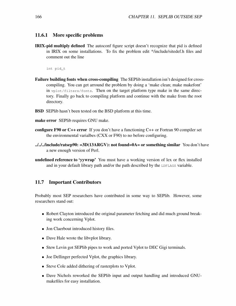
166 CHAPTER 11. SEPLIB OUTSIDE SEP
11.6.1 More specific problems
IRIX-pid multiply defined The autoconf figure script doesn’t recognize that pid is definedin IRIX on some installations. To fix the problem edit */include/sitedef.h files andcomment out the line
int pid_t
Failure building fonts when cross-compiling The SEPlib installation isn’t designed for cross-compiling. You can get arround the problem by doing a ‘make clean; make makefont’in vplot/filters/fonts. Then on the target platform type make in the same direc-tory. Finally go back to compiling platform and continue with the make from the rootdirectory.
BSD SEPlib hasn’t been tested on the BSD platform at this time.
make error SEPlib requires GNU make.
configure F90 or C++ error If you don’t have a functioning C++ or Fortran 90 compiler setthe environmental varialbes (CXX or F90) to no before configuring.
../../../include/ratsep90: =3D(13ARGV): not found=0A= or something similar You don’t havea new enough version of Perl.
undefined reference to ‘yywrap’ You must have a working version of lex or flex installedand in your default library path and/or the path described by the LDFLAGS variable.
11.7 Important Contributors
Probably most SEP researchers have contributed in some way to SEPlib. However, someresearchers stand out:
• Robert Clayton introduced the original parameter fetching and did much ground break-ing work concerning Vplot.
• Jon Claerbout introduced history files.
• Dave Hale wrote the libvplot library.
• Stew Levin got SEPlib pipes to work and ported Vplot to DEC Gigi terminals.
• Joe Dellinger perfected Vplot, the graphics library.
• Steve Cole added dithering of rasterplots to Vplot.
• Dave Nichols reworked the SEPlib input and output handling and introduced GNU-makefiles for easy installation.

11.7. IMPORTANT CONTRIBUTORS 167
• Martin Karrenbach had a first SEPlib extension to handle irregular data.
• Bob Clapp and Biondo Biondi (with the help of current SEP students) truly extendedSEPlib to handle irregular data (SEP3D).
• Sergey Fomel and Paul Sava have made recent additions to the traveltime/ray tracingabilities of SEPlib.
REFERENCES
Claerbout, J. F., 1992, Earth Soundings Analysis: Processing versus Inversion: BlackwellScientific Publications.
Claerbout, J. Geophysical Estimation by Example: Environmental soundings image enhance-ment:. http://sepwww.stanford.edu/sep/prof/, 1998.

168 CHAPTER 11. SEPLIB OUTSIDE SEP
REFERENCES
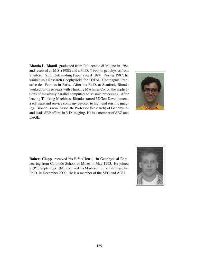
Biondo L. Biondi graduated from Politecnico di Milano in 1984and received an M.S. (1988) and a Ph.D. (1990) in geophysics fromStanford. SEG Outstanding Paper award 1994. During 1987, heworked as a Research Geophysicist for TOTAL, Compagnie Fran-caise des Petroles in Paris. After his Ph.D. at Stanford, Biondoworked for three years with Thinking Machines Co. on the applica-tions of massively parallel computers to seismic processing. Afterleaving Thinking Machines, Biondo started 3DGeo Development,a software and service company devoted to high-end seismic imag-ing. Biondo is now Associate Professor (Research) of Geophysicsand leads SEP efforts in 3-D imaging. He is a member of SEG andEAGE.
Robert Clapp received his B.Sc.(Hons.) in Geophysical Engi-neering from Colorado School of Mines in May 1993. He joinedSEP in September 1993, received his Masters in June 1995, and hisPh.D. in December 2000. He is a member of the SEG and AGU.
169
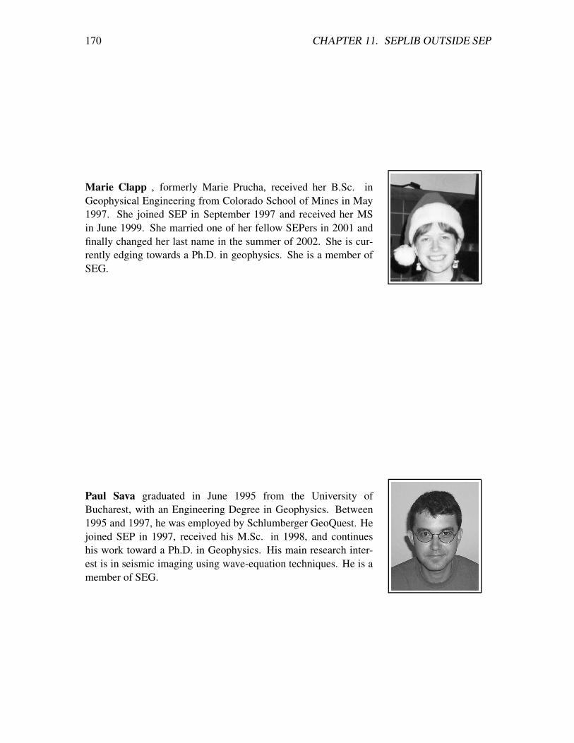
170 CHAPTER 11. SEPLIB OUTSIDE SEP
Marie Clapp , formerly Marie Prucha, received her B.Sc. inGeophysical Engineering from Colorado School of Mines in May1997. She joined SEP in September 1997 and received her MSin June 1999. She married one of her fellow SEPers in 2001 andfinally changed her last name in the summer of 2002. She is cur-rently edging towards a Ph.D. in geophysics. She is a member ofSEG.
Paul Sava graduated in June 1995 from the University ofBucharest, with an Engineering Degree in Geophysics. Between1995 and 1997, he was employed by Schlumberger GeoQuest. Hejoined SEP in 1997, received his M.Sc. in 1998, and continueshis work toward a Ph.D. in Geophysics. His main research inter-est is in seismic imaging using wave-equation techniques. He is amember of SEG.