Separating Signal from Noise in Global Warming

Bert W. Rust

Reprinted from the CD

Rust, B. W. (2003) “Separating Signal from Noise in Global Warming,” ComputingScience and Statistics, 35, 263-277.

– or –

Rust, B. W. (2003) “Separating Signal from Noise in Global Warming,” ComputingScience and Statistics, 35, I2003Proceedings/RustBert/RustBert.paper.pdf

Separating Signal from Noise in Global Warming

Bert W. Rust

Mathematical and Computational Sciences Division

National Institute of Standards and Technology

100 Bureau Drive, Stop 8910

Gaithersburg, MD 20899-8910

bwr@cam.nist.gov

July 23, 2003

Abstract

One argument often used against global warming is that the global tem-perature record is too noisy to allow a clear determination of the signal. Thispaper presents two models for the signal which suggest that: (1) the warmingis accelerating, (2) the warming is related to the growth in fossil fuel emissions,and (3) the warming in the last 146 years has been at least 10 times greaterthan the noise level. One model uses a constant rate for the acceleration andthe other an exponential whose rate constant is exactly one half that of thegrowth in fossil fuel emissions. The two models can be viewed as best case andworst case scenarios for extrapolations into the future, but the data measuredso far cannot reliably distinguish between them.

1 Introduction

Measurements by C. D. Keeling and his colleagues [7] at the Mauna Loa Observatoryin Hawaii show that in the years 1959-2001 the atmospheric CO2 concentration hasrisen from 316 to 371 parts per million by volume, an increase of 17.4%. Themain source of this increase is thought to be fossil fuel emissions. Since CO2 is astrong greenhouse gas, it is generally agreed that these additions to the atmosphereshould produce some global warming, but there is considerable disagreement overthe magnitude of the effect.

Figure 1 is a plot of annual global average tropospheric temperature anomalies(relative to the average for 1961-1990) for the years 1856-2001. These data werecomputed and tabulated by P. D. Jones and his colleagues [5, 6] at the ClimaticResearch Unit of the University of East Anglia. They can be obtained online athttp://www.cru.uea.ac.uk/cru/cru.htm. The horizontal lines indicate the averageanomaly ± one standard deviation, i.e., (−0.145 ± 0.231) ◦C. Before 1980, it waspossible to argue that the apparent increase was too small, relative to the scatterin the data, to indicate a systematic trend, but measurements over the last twodecades have removed much of the doubt about the warming.

263

264 B. W. Rust

Figure 1: Annual global average temperature anomalies (1856-2001). Each anomalyis the average temperature for that year minus the average for the period 1961-1990.

2 Polynomial Models

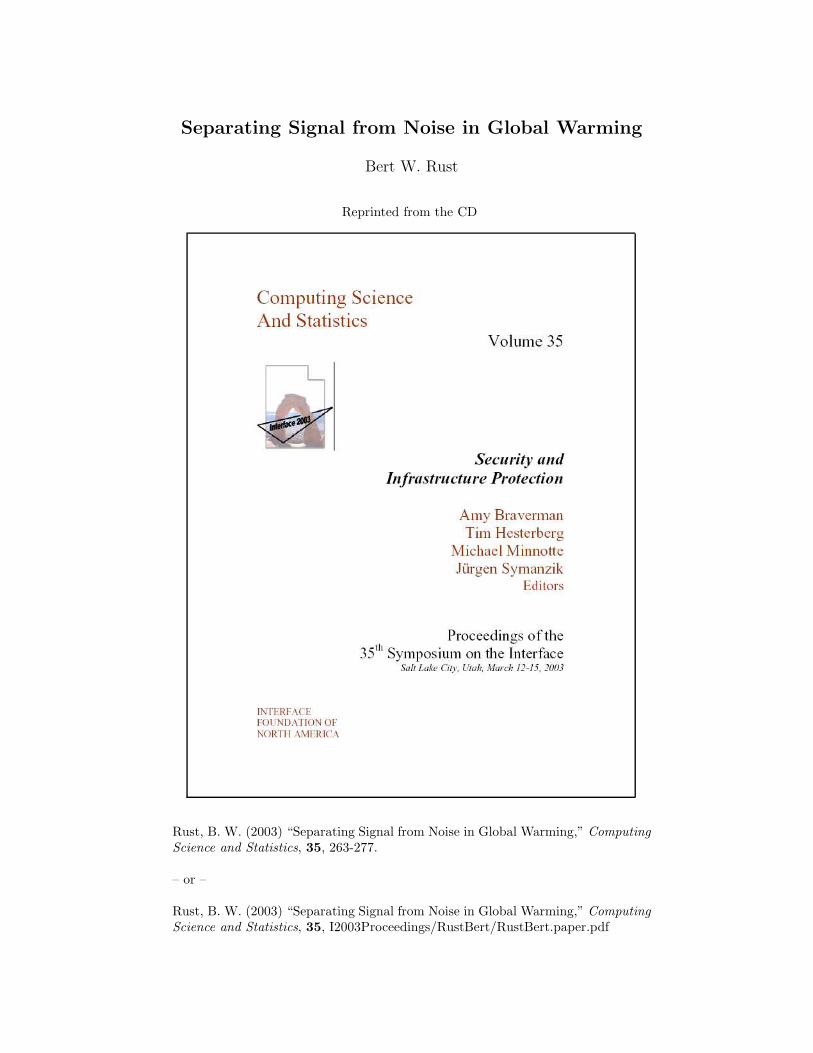
Figure 2 gives a plot of the least squares fit of the straight line model

T (t − t0) = T0 + C1(t − t0) , with t0 ≡ 1856.0 , (1)

where t is time (measured in years A.D.) and T is temperature anomaly (measuredin ◦C). For all of the fits in this paper, the zero point of the time scale was shiftedto epoch 1856.0, which is the beginning of the record, and each yearly average wasassigned to the mid-point of its corresponding year. The parameters estimates were

T0 = (−0.463± .023) [◦C] , C1 = (4.36± .28) × 10−3 [◦C/yr] . (2)

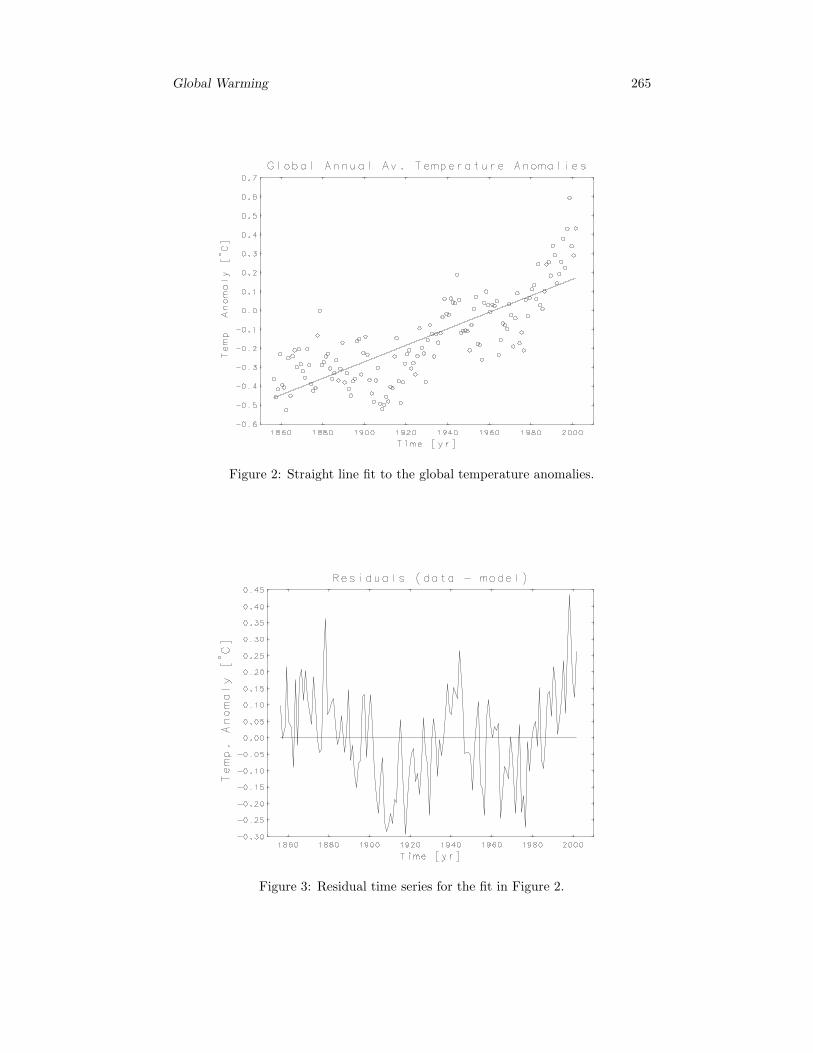
The residual time series, shown in Figure 3, exhibits a quasi-periodic oscillationabout a concave upward base line. The last property is not obvious by inspectionbut is strikingly confirmed by a Fourier power (variance) spectrum. Figure 4 givesthe periodogram of the residuals, truncated at frequency 0.10 yr−1 rather than0.50 yr−1 because there were no high frequeny features comparable to the twolow frequency peaks. The periods corresponding to the centers of those peaks areτ0 ≈ 143 years and τ1 ≈ 62.5 years. Since the total length of the time series wasonly 146 years, the first peak is an obvious indicator that the straight line is aninadequate base line.

If the straight line, which represents warming with a constant rate C1, will notdo, then the next logical candidate for a base line is a quadratic

T (t − t0) = T0 + C1(t − t0) + C2(t − t0)2 , (3)

which represents warming with a constant acceleration C2. The least squares esti-mates for this model were

T0 = −0.311± .031 [◦C] , C1 = (−1.88± .97) × 10−3 [◦C/yr] ,

C2 = (4.27± .64) × 10−5 [◦C/yr2] .(4)

Global Warming 265

Figure 2: Straight line fit to the global temperature anomalies.

Figure 3: Residual time series for the fit in Figure 2.

266 B. W. Rust

Figure 4: Truncated (in frequency) periodogram for the residuals in Figure 3.

The relatively large uncertainty in C1 suggests that a reduced quadratic model

T (t − t0) = T0 + C2(t − t0)2 (5)

might be indicated by the data. The estimates for that fit were

T0 = −0.363± .015 [◦C] , C2 = (3.06± .16) × 10−5 [◦C/yr2] , (6)

and a formal F-test accepts the null hypothesis C1 = 0 at the 95% level of signifi-cance [11]. Thus, the data seem to demand a monotonically increasing, acceleratedwarming. Figure 5 shows both fits, and Figure 6 shows the residual time series forthe reduced quadratic fit.

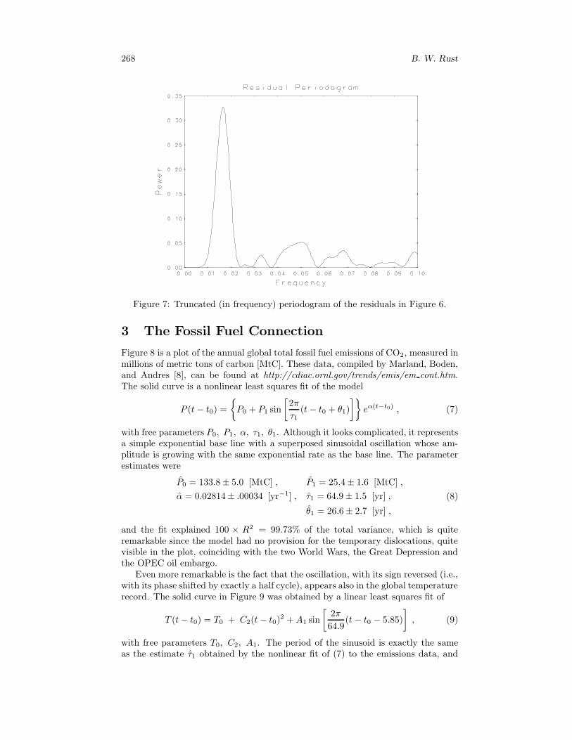
Figure 7 gives the periodogram of the residuals in Figure 6. It is dominatedby a single peak whose central frequency corresponds to a period τ1 ≈ 61.5 years.Since there are ≈2.4 repetitions of this cycle in the record, it almost certainlyrepresents a real oscillation. Attempts [10, 11] to accomodate this variation byfitting higher order polynomials were ineffective for polynomials of order 3 and 4.That is, no statistically significant reduction in the sum of squared residuals wasobtained, and the uncertainties in the parameter estimates were almost as large asthe estimates themselves. That situation changed for a 5th order polynomial (6 freeparameters) which was able to capture the variation, with statistical significance,but high order polynomial behavior is rare in nature whereas cycles are ubiquitous.And this particular cycle has previously been noted by Mitchell [9], who was usingan older, cruder temperture record, and by Schlesinger and Ramankutty [16], whosuggested that “the oscillation arises from predictable internal variability of theocean-atmosphere system.” Even though the cause of the cycle is not known, it isvery important because a cycle with the same period occurs in the record of fossilfuel CO2 emissions which are widely thought to be driving the global warming.

Global Warming 267

Figure 5: Fits of the full quadratic model (3) and the reduced quadratic model (5)to the global temperature anomalies.

Figure 6: Residual time series for the reduced quadratic fit in Figure 5.

268 B. W. Rust

Figure 7: Truncated (in frequency) periodogram of the residuals in Figure 6.

3 The Fossil Fuel Connection

Figure 8 is a plot of the annual global total fossil fuel emissions of CO2, measured inmillions of metric tons of carbon [MtC]. These data, compiled by Marland, Boden,and Andres [8], can be found at http://cdiac.ornl.gov/trends/emis/em cont.htm.The solid curve is a nonlinear least squares fit of the model

P (t − t0) =

{

P0 + P1 sin

[

2π

τ1(t − t0 + θ1)

]}

eα(t−t0) , (7)

with free parameters P0, P1, α, τ1, θ1. Although it looks complicated, it representsa simple exponential base line with a superposed sinusoidal oscillation whose am-plitude is growing with the same exponential rate as the base line. The parameterestimates were

P0 = 133.8± 5.0 [MtC] , P1 = 25.4± 1.6 [MtC] ,

α = 0.02814± .00034 [yr−1] , τ1 = 64.9± 1.5 [yr] ,

θ1 = 26.6± 2.7 [yr] ,

(8)

and the fit explained 100 × R2 = 99.73% of the total variance, which is quiteremarkable since the model had no provision for the temporary dislocations, quitevisible in the plot, coinciding with the two World Wars, the Great Depression andthe OPEC oil embargo.

Even more remarkable is the fact that the oscillation, with its sign reversed (i.e.,with its phase shifted by exactly a half cycle), appears also in the global temperaturerecord. The solid curve in Figure 9 was obtained by a linear least squares fit of

T (t − t0) = T0 + C2(t − t0)2 + A1 sin

[

2π

64.9(t − t0 − 5.85)

]

, (9)

with free parameters T0, C2, A1. The period of the sinusoid is exactly the sameas the estimate τ1 obtained by the nonlinear fit of (7) to the emissions data, and

Global Warming 269

Figure 8: Annual global total fossil fuel CO2 emissions. The curve is the fit of theexponential/sinusoidal model (7).

Figure 9: Fits of the quadratic/sinusoidal model (9) and the exponential/sinusoidalmodel (10) to the global temperature anomalies.

270 B. W. Rust

the phase constant -5.85 has been set to make the oscillation exactly one half cycleahead (or behind) the one obtained for that fit. Thus, maxima in the temperatureoscillation correspond to minima in the emissions oscillation and vice versa. Thisinverse correlation has previously been noted by Rust and Kirk [15] and Rust andCrosby [14] who argued that it might represent a Gaiaen feedback by which in-creasing temperatures would cause reductions in fossil fuel production. That maybe wishful thinking, however, and it must be admitted that the cause of the os-cillation is unknown. But its occurrence in both records is strong evidence for aconnection between the warming and the fossil fuel emissions.

We have seen that the temperature data seem to demand a monotonically in-creasing base line which we modelled with the reduced quadratic (5). But the dataare fit just as well by an exponential base line whose rate constant is exactly onehalf of the α obtained by fitting (7) to the emissions data. The dashed curve inFigure 9 was obtained by a linear least squares fit of

T (t − t0) = T0 + C2 exp [0.01407(t− t0)] + A1 sin

[

2π

64.9(t − t0 − 5.85)

]

, (10)

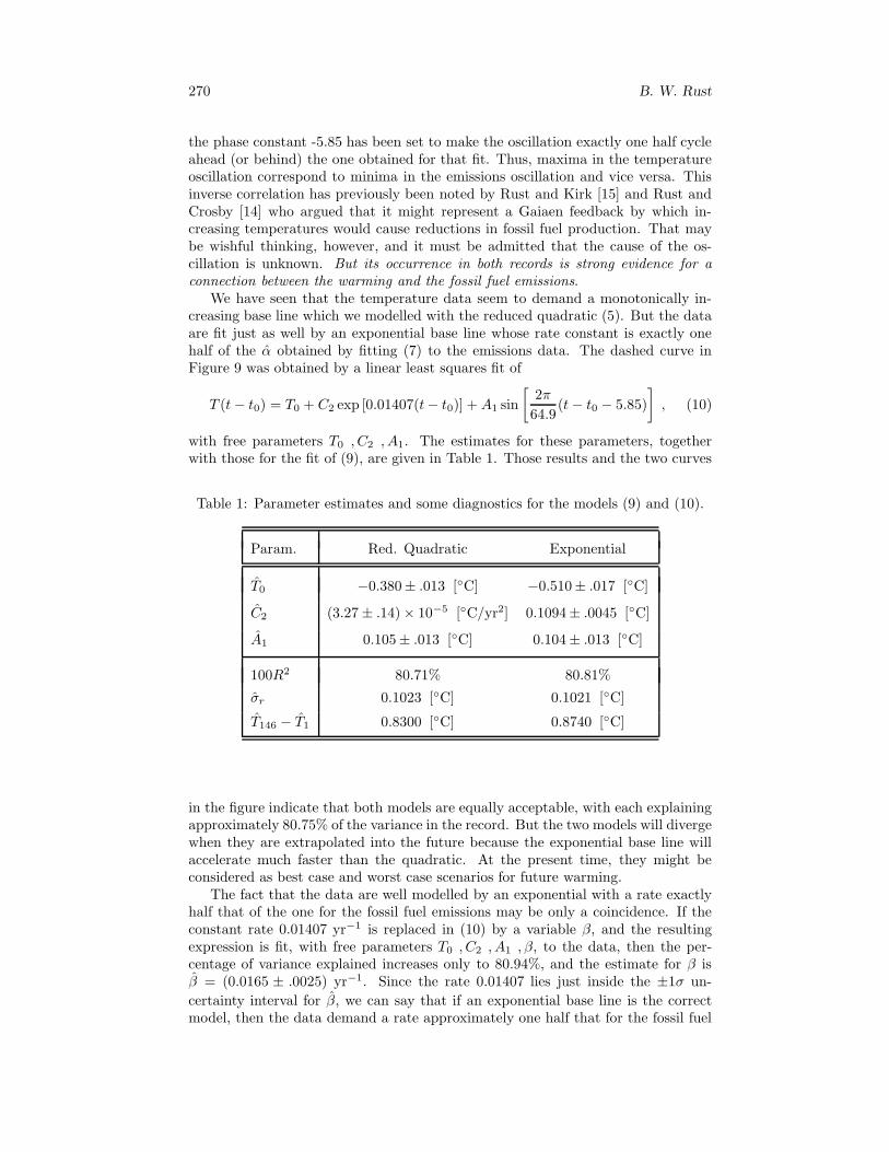
with free parameters T0 , C2 , A1. The estimates for these parameters, togetherwith those for the fit of (9), are given in Table 1. Those results and the two curves

Table 1: Parameter estimates and some diagnostics for the models (9) and (10).

Param. Red. Quadratic Exponential

T0 −0.380± .013 [◦C] −0.510± .017 [◦C]

C2 (3.27 ± .14) × 10−5 [◦C/yr2] 0.1094± .0045 [◦C]

A1 0.105± .013 [◦C] 0.104± .013 [◦C]

100R2 80.71% 80.81%

σr 0.1023 [◦C] 0.1021 [◦C]

T146 − T1 0.8300 [◦C] 0.8740 [◦C]

in the figure indicate that both models are equally acceptable, with each explainingapproximately 80.75% of the variance in the record. But the two models will divergewhen they are extrapolated into the future because the exponential base line willaccelerate much faster than the quadratic. At the present time, they might beconsidered as best case and worst case scenarios for future warming.

The fact that the data are well modelled by an exponential with a rate exactlyhalf that of the one for the fossil fuel emissions may be only a coincidence. If theconstant rate 0.01407 yr−1 is replaced in (10) by a variable β, and the resultingexpression is fit, with free parameters T0 , C2 , A1 , β, to the data, then the per-centage of variance explained increases only to 80.94%, and the estimate for β isβ = (0.0165 ± .0025) yr−1. Since the rate 0.01407 lies just inside the ±1σ un-

certainty interval for β, we can say that if an exponential base line is the correctmodel, then the data demand a rate approximately one half that for the fossil fuel

Global Warming 271

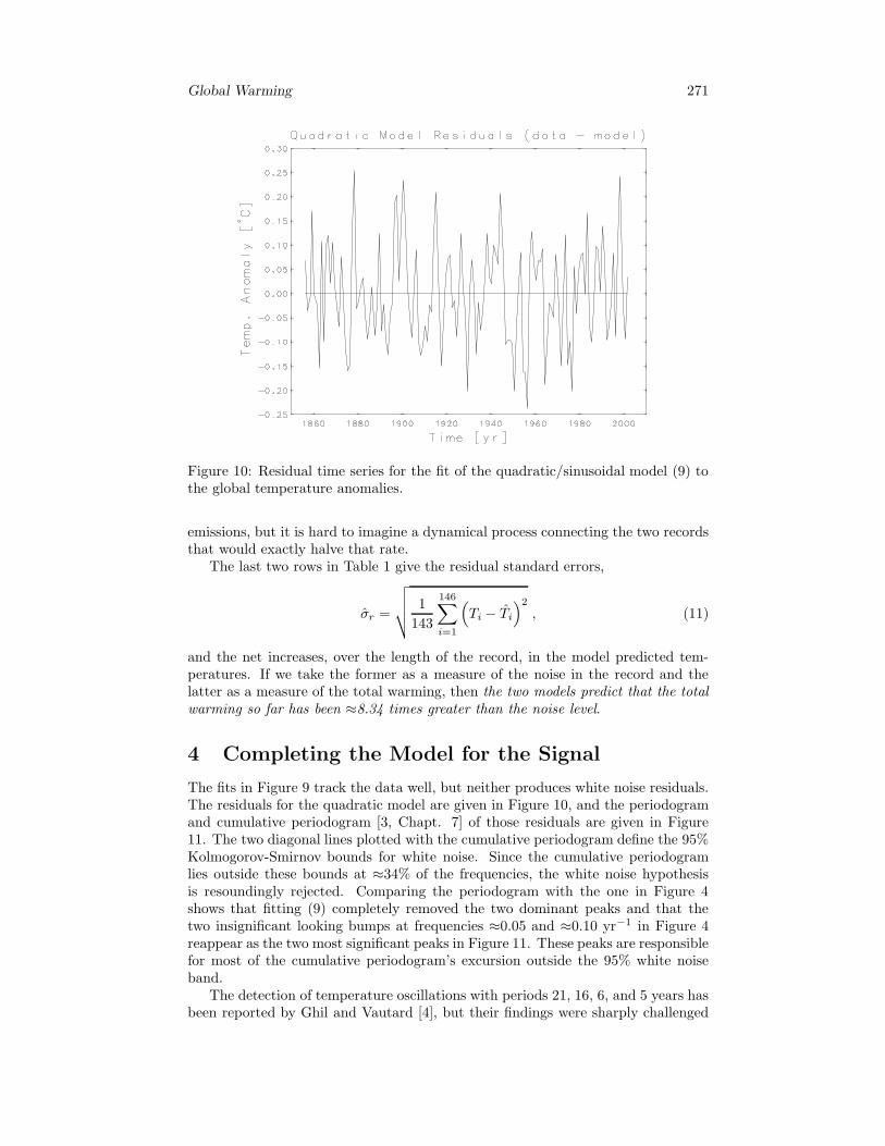
Figure 10: Residual time series for the fit of the quadratic/sinusoidal model (9) tothe global temperature anomalies.

emissions, but it is hard to imagine a dynamical process connecting the two recordsthat would exactly halve that rate.

The last two rows in Table 1 give the residual standard errors,

σr =

√

√

√

√

1

143

146∑

i=1

(

Ti − Ti

)2

, (11)

and the net increases, over the length of the record, in the model predicted tem-peratures. If we take the former as a measure of the noise in the record and thelatter as a measure of the total warming, then the two models predict that the totalwarming so far has been ≈8.34 times greater than the noise level.

4 Completing the Model for the Signal

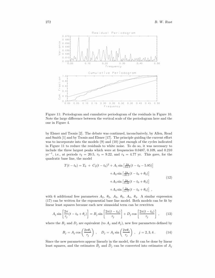
The fits in Figure 9 track the data well, but neither produces white noise residuals.The residuals for the quadratic model are given in Figure 10, and the periodogramand cumulative periodogram [3, Chapt. 7] of those residuals are given in Figure11. The two diagonal lines plotted with the cumulative periodogram define the 95%Kolmogorov-Smirnov bounds for white noise. Since the cumulative periodogramlies outside these bounds at ≈34% of the frequencies, the white noise hypothesisis resoundingly rejected. Comparing the periodogram with the one in Figure 4shows that fitting (9) completely removed the two dominant peaks and that thetwo insignificant looking bumps at frequencies ≈0.05 and ≈0.10 yr−1 in Figure 4reappear as the two most significant peaks in Figure 11. These peaks are responsiblefor most of the cumulative periodogram’s excursion outside the 95% white noiseband.

The detection of temperature oscillations with periods 21, 16, 6, and 5 years hasbeen reported by Ghil and Vautard [4], but their findings were sharply challenged

272 B. W. Rust

Figure 11: Periodogram and cumulative periodogram of the residuals in Figure 10.Note the large difference between the vertical scale of the periodogram here and theone in Figure 4.

by Elsner and Tsonis [2]. The debate was continued, inconclusively, by Allen, Readand Smith [1] and by Tsonis and Elsner [17]. The principle guiding the current effortwas to incorporate into the models (9) and (10) just enough of the cycles indicatedin Figure 11 to reduce the residuals to white noise. To do so, it was necessary toinclude the three largest peaks which were at frequencies 0.0487, 0.109, and 0.210yr−1, i.e., at periods τ2 = 20.5, τ3 = 9.22, and τ4 = 4.77 yr. This gave, for thequadratic base line, the model

T (t − t0) = T0 + C2(t − t0)2 + A1 sin

[

2π64.9 (t − t0 − 5.85)

]

+A2 sin[

2π20.5(t − t0 + θ2)

]

+A3 sin[

2π9.22(t − t0 + θ3)

]

+A4 sin[

2π4.77(t − t0 + θ4)

]

,

(12)

with 6 additional free parameters A2, θ2, A3, θ3, A4, θ4. A similar expression(17) can be written for the exponential base line model. Both models can be fit bylinear least squares because each new sinusoidal term can be rewritten

Aj sin

[

2π

τj

(t − t0 + θj)

]

= Bj sin

[

2π(t − t0)

τj

]

+ Dj cos

[

2π(t − t0)

τj

]

, (13)

where the Bj and Dj are equivalent (to Aj and θj), new free parameters defined by

Bj = Aj cos

(

2πθj

τj

)

, Dj = Aj sin

(

2πθj

τj

)

, j = 2, 3, 4 . (14)

Since the new parameters appear linearly in the model, the fit can be done by linearleast squares, and the estimates Bj and Dj can be converted into estimates of Aj

Global Warming 273

and θj by the inverse relations

Aj = +

√

B2 + D2 , θ =τj

2πtan−1

(

Dj

Bj

)

, j = 2, 3, 4 . (15)

More details on the use of these tranformations and on converting the uncertaintiesin the Bj and Dj to equivalent uncertainties in the Aj and θj can be found in tworecent tutorial papers by Rust [12, 13].

Some of the parameter estimates and statistics for the fit of of the expandedmodel (12) are given in Table 2, together with the estimates for the simpler model

(9) for comparison. The estimated phase shifts θ2, θ3, θ4 were not included because

Table 2: Parameter estimates and some diagnostics for the models (9) and (12).

Param. 3-Param. Model 9-Param. Model

T0 −0.380± .013 [◦C] −0.382± .012 [◦C]

C2 (3.27± .14) × 10−5 [◦C/yr2] (3.28 ± .12)× 10−5 [◦C/yr2]

A1 0.105± .013 [◦C] 0.106± .011 [◦C]

A2 0.041± .011 [◦C]

A3 0.042± .011 [◦C]

A4 0.033± .011 [◦C]

SSR 1.4975 [◦C2] 1.1576 [◦C2]

100R2 80.71% 85.09%

σr 0.1023 [◦C] 0.09192 [◦C]

T146 − T1 0.8300 [◦C] 0.9193 [◦C]

their uncertainties are not reliable indicators of the significance of the cycles. Theestimated amplitudes A2 , A3 , A4 and their uncertainties do indicate the strengthof the cycles, and in all three cases the amplitudes are at least 3 times larger thantheir corresponding uncertainties. This suggests statistical significance, and thestandard F-test confirms that the 6 new free parameters do produce a significantreduction in the sum of squared residuals. Let the null hypothesis be H0 : A2 =A3 = A4 = θ2 = θ3 = θ4 = 0. Then, with m = 146, n = 9, and k = 6 we have

u =(SSR)H − (SSR)F

(SSR)F

×m − n

k= 6.703 > 2.165 = F0.95(k, m − n) , (16)

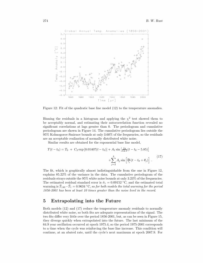
so H0 is rejected.The fit is shown in Figure 12. Although the three new oscillations are not readily

discernable in the data, they are quite obvious in the fit, so they look somewhatcontrived. But a good argument for their reality is the fact that including themreduces the residuals, shown in Figure 13, to normally distributed white noise.

274 B. W. Rust

Figure 12: Fit of the quadratic base line model (12) to the temperature anomalies.

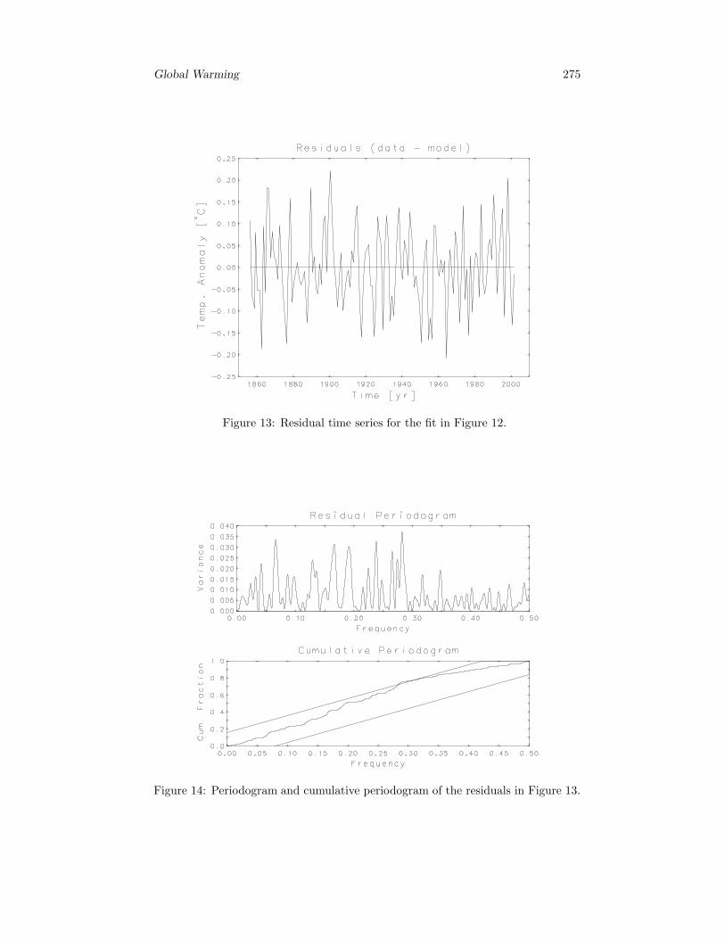
Binning the residuals in a histogram and applying the χ2 test showed them tobe acceptably normal, and estimating their autocorrelation function revealed nosignificant correlations at lags greater than 0. The periodogram and cumulativeperiodogram are shown in Figure 14. The cumulative periodogram lies outside the95% Kolmogorov-Smirnov bounds at only 3.60% of the frequencies, so the residualsare an acceptable realization of normally distributed white noise.

Similar results are obtained for the exponential base line model,

T (t − t0) = T0 + C2 exp [0.01407(t− t0)] + A1 sin[

2π64.9 (t − t0 − 5.85)

]

+

4∑

j=2

Aj sin[

2πτj

(t − t0 + θj)]

.(17)

The fit, which is graphically almost indistinguishable from the one in Figure 12,explains 85.22% of the variance in the data. The cumulative periodogram of theresiduals strays outside the 95% white noise bounds at only 3.23% of the frequencies.The estimated residual standard error is σr = 0.09152 ◦C, and the estimated totalwarming is T146−T1 = 0.9634 ◦C, so for both models the total warming for the period1856-2001 has been at least 10 times greater than the noise level in the record.

5 Extrapolating into the Future

Both models (12) and (17) reduce the temperature anomaly residuals to normallydistributed white noise, so both fits are adequate representations of the signal. Thetwo fits differ very little over the period 1856-2001, but, as can be seen in Figure 15,they diverge quickly when extrapolated into the future. The last minimum of the64.9 year oscillation occurred at epoch 1975.4, so the period 1975-2001 correspondsto a time when the cycle was reinforcing the base line increase. This condition willcontinue, at an abated rate, until the cycle’s next maximum at epoch 2007.9. For

Global Warming 275

Figure 13: Residual time series for the fit in Figure 12.

Figure 14: Periodogram and cumulative periodogram of the residuals in Figure 13.

276 B. W. Rust

Figure 15: One hundred year extrapolations for the two models (12) and (17).

the next 32.5 years after that, the cycle will decline and partially offset the baseline increase, an effect clearly visible in the quadratic extrapolation, but less so inthe exponential extrapolation. After that the exponential increases so rapidly thatthe oscillation is scarcely discernible.

These extrapolations assume that the dynamics causing the signals will continueunchanged into the future. Fossil fuel reserves are probably sufficient to support acontinuation of the exponential growth observed in Figure 8, though doing so mightrequire massive switches from petroleum fuels back to coal and its derivatives. Thecauses of the 64.9 year oscillations are unknown, but their persistence and coherencein both records for 2.25 cycles certainly suggest stability. But there remains thepossibility that warming might trigger other events which would produce positivefeedbacks. For example, an extensive thawing of the permafrost in the Arctic and/orthe ignition of peat in the soil by hot forest fires in the tropical and temperate regionsmight add new transfers of CO2 to the atmosphere which would not be subject tohuman control. Such events might have disasterous consequences, especially if theexponential base line scenario is correct.

6 Acknowledgments

The author would like to thank Drs. Isabel Beichl, R. F. Boisvert and AnastaseNakassis for their helpful reviews and suggestions for improving this paper.

References

[1] Allen, M. R., Read, P. L., and Smith, L. A. (1992) “Temperature time-series?,”Nature, Vol. 355, p. 686.

[2] Elsner, J. B. and Tsonis, A. A. (1991) “Do bidecadal oscillations exist in theglobal temperature record?” Nature, Vol. 353, pp. 551-553.

Global Warming 277

[3] Fuller, W. A. (1976) Introduction to Statistical Time Series, John Wiley &Sons, New York, pp. 275-287.

[4] Ghil, M. and Vautard, R. (1991) “Interdecadal oscillations and the warmingtrend in global temperature time series,” Nature, vol. 350, pp. 324-327.

[5] Jones, P. D., Osborn, T. J., Briffa, K. R., Folland, C. K., Horton, B., Alexander,L. V., Parker, D. E. and Rayner, N. A. (2001) “Adjusting for sampling densityin grid-box land and ocean surface temperature time series,” J. Geophys. Res.,vol. 106, pp. 3371-3380.

[6] Jones, P. D. and Moberg, A. (2003) “Hemispheric and large-scale surface airtemperature variations: An extensive revision and an update to 2001,” J. Cli-mate, vol. 16, pp. 206-223.

[7] Keeling, C. D. and Whorf, T. P. (2003) “Atmospheric carbon dioxide recordfrom Mauna Loa,” in Online Trends: A Compendium of Data on Global Change(http://cdiac.ornl.gov/trends/co2/contents.htm). Carbon Dioxide InformationAnalysis Center, Oak Ridge National Laboratory, Oak Ridge, Tennessee.

[8] Marland, G., Boden, T. A. and Andres, R. J. (2000) “Global, Regional, andNational CO2 Emissions,” Trends: A Compendium of Data on Global Change.CDIAC, ORNL, Oak Ridge, TN.

[9] Mitchell, Jr, J. M. (1963) “On the world-wide pattern of secular temperaturechange,” Changes of Climate, UNESCO, Paris, pp. 161-181.

[10] Rust, B. W. (2001) “Fitting nature’s basic functions Part I: polynomials andlinear least squares,” Computing in Science & Engineering, Vol. 3, no. 5, pp.84-89.

[11] Rust, B. W. (2001) “Fitting nature’s basic functions Part II: estimating uncer-tainties and testing hypotheses,” Computing in Science & Engineering, Vol. 3,no. 6, pp. 60-64.

[12] Rust, B. W. (2002) “Fitting nature’s basic functions Part III: exponentials,sinusoids, and nonlinear least squares,” Computing in Science & Engineering,Vol. 4, no. 4, pp. 72-77.

[13] Rust, B. W. (2003) “Fitting nature’s basic functions Part IV:the variable pro-jection algorithm,” Computing in Science & Engineering, Vol. 5, no. 2, pp.74-79.

[14] Rust B. W. and Crosby, F. J. (1994) “Further studies on the modulation of fossilfuel production by global temperature variations,” Environment International,vol. 20, no. 4, pp. 429-456.

[15] Rust B. W. and Kirk, B. L. (1982) “Modulation of fossil fuel production byglobal temperature variations,” Environment International, vol. 7, pp. 419-422.

[16] Schesinger, M. E. and Ramankutty, N. (1994) “An oscillation in the globalclimate system of period 65-70 years,” Nature, Vol. 367, pp. 723-726.

[17] Tsonis, A. A. and Elsner, J. B. (1992) “Oscillating global temperature,” Nature,Vol.356, p. 751.