Embed Size (px)
Citation preview

September 24, 2001 L5.1
Introduction to Algorithms6.046
Lecture 6Prof. Shafi Goldwasser

How fast can we sort?All the sorting algorithms we have seen so far are comparison sorts: only use comparisons to determine the relative order of elements.•E.g., insertion sort, merge sort, quicksort,
heapsort.
The best worst-case running time that we’ve seen for comparison sorting is O(n lg n) .Q:Is O(n lg n) the best we can do?A: Yes, as long as we use comparison sorts
TODAY: Prove any comparison sort has (n long) worst case running time

The Time Complexity of a Problem The minimum time needed by an algorithm to solve it.
Problem P is solvable in time Tupper(n) if there is an algorithm A which
• outputs the correct answer • in this much time
Eg: Sorting computable in Tupper(n) = O(n2) time.
A, I, A(I)=P(I) and Time(A,I) Tupper(|I|)
Upper Bound:

The Time Complexity of a Problem The minimum time needed by an algorithm to solve it.
Time Tlower(n) is a lower bound for problem
if no algorithm solve the problem faster.
There may be algorithms that give the correct answer or run quickly on some inputs instance.
Lower Bound:

The Time Complexity of a Problem The minimum time needed by an algorithm to solve it.
Lower Bound: Time Tupper(n) is a lower bound for problem P
if no algorithm solve the problem faster.
Eg: No algorithm can sort N values in Tlower = sqrt(N) time.
But for every algorithm, there is at least one instance I for which either the algorithm gives the wrong answer or it runs in too much time. A, I, A(I) P(I) or Time(A,I) Tlower(|I|)

A, I, A(I)=P(I) and Time(A,I) Tupper(|I|)
A, I, A(I) P(I) or Time(A,I) Tlower(|I|)Lower Bound:
Upper Bound:
The Time Complexity of a Problem The minimum time needed by an algorithm to solve it.
“There is” and “there isn’t a faster algorithm”are almost negations of each other.

A, I, A(I)=P(I) and Time(A,I) Tupper(|I|)Upper Bound:
Prover-Adversary Game
I have an algorithm A that I claim works and is fast.
I win if A on input I gives •the correct output •in the allotted time.
Oh yeah, I have an input I for which it does not.
What we have been doing all along.

Lower Bound:
Prover-Adversary Game
I win if A on input I gives •the wrong output or •runs slow.
A, I, [ A(I) P(I) or Time(A,I) Tlower(|I|)]
Proof by contradiction.
I have an algorithm A that I claim works and is fast.
Oh yeah, I have an input I for which it does not .

Lower Bound:
Prover-Adversary Game
A, I, [ A(I) P(I) or Time(A,I) Tlower(|I|)]
I have an algorithm A that I claim works and is fast.
Lower bounds are very hard to prove, because I must consider every algorithm no matter how strange.

Today:
Prove a Lower Bound for any comparison based algorithm for the Sorting Problem
How?Decision trees help us.

Decision-tree example
1:2
2:3
123 1:3
132 312
1:3
213 2:3
231 321
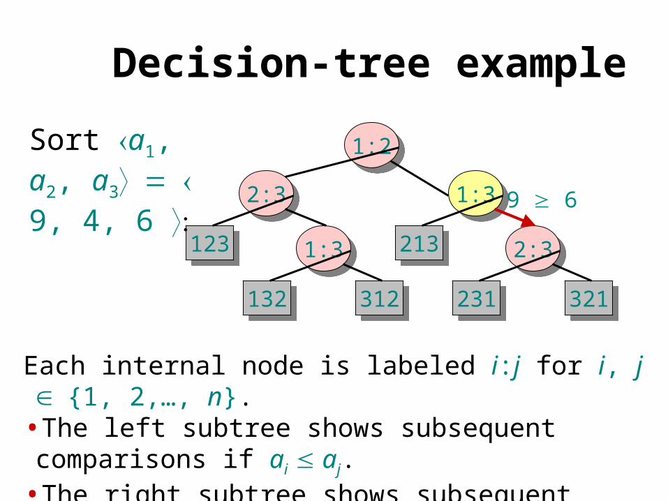
Each internal node is labeled i:j for i, j {1, 2,…, n}.•The left subtree shows subsequent comparisons if ai aj.
•The right subtree shows subsequent comparisons if ai aj.
Sort a1, a2, …, an

Decision-tree example
1:2
2:3
123 1:3
132 312
1:3
213 2:3
231 321
Each internal node is labeled i:j for i, j {1, 2,…, n}.•The left subtree shows subsequent comparisons if ai aj.
•The right subtree shows subsequent comparisons if ai aj.
9 4Sort a1, a2, a3 9, 4, 6
Decision-tree example
1:2
2:3
123 1:3
132 312
1:3
213 2:3
231 321
Each internal node is labeled i:j for i, j {1, 2,…, n}.•The left subtree shows subsequent comparisons if ai aj.
•The right subtree shows subsequent comparisons if ai aj.
9 6
Sort a1, a2, a3 9, 4, 6

Decision-tree example
1:2
2:3
123 1:3
132 312
1:3
213 2:3
231 321
Each internal node is labeled i:j for i, j {1, 2,…, n}.•The left subtree shows subsequent comparisons if ai aj.
•The right subtree shows subsequent comparisons if ai aj.
4 6
Sort a1, a2, a3 9, 4, 6

Decision-tree example
1:2
2:3
123 1:3
132 312
1:3
213 2:3
231 321
Each leaf contains a permutation , ,…, (n) to indicate that the ordering a(1) a(2) a(n) has been established.
4 6 9
Sort a1, a2, a3 9, 4, 6

Decision-tree model
A decision tree can model the execution of any comparison sort:•One tree for each input size n. •View the algorithm as splitting whenever
it compares two elements.•The tree contains the comparisons along
all possible instruction traces.•The running time of the algorithm = the
length of the path taken.•Worst-case running time = height of tree.

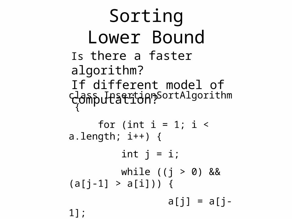
class InsertionSortAlgorithm {
for (int i = 1; i < a.length; i++) {
int j = i;
while ((j > 0) && (a[j-1] > a[i])) {
a[j] = a[j-1];
j--; }
a[j] = B; }}
Any comparison sortCan be turned into a Decision tree
1:2
2:3
123 1:3
132 312
1:3
213 2:3
231 321

Lower bound for decision-tree sorting
Theorem. Any decision tree that can sort n elements must have height (n lg n) .
Proof. The tree must contain n! leaves, since there are n! possible permutations. A height-h binary tree has 2h leaves. Thus, n! 2h . h lg(n!) (lg is mono. increasing)
lg ((n/e)n) (Stirling’s formula)= n lg n – n lg e= (n lg n) .

Lower bound for comparison sorting
Corollary. Heapsort and merge sort are asymptotically optimal comparison sorting algorithms.
class InsertionSortAlgorithm {
for (int i = 1; i < a.length; i++) {
int j = i;
while ((j > 0) && (a[j-1] > a[i])) {
a[j] = a[j-1];
j--; }
a[j] = B; }}
Is there a faster algorithm?If different model of computation?
SortingLower Bound

Sorting in linear time
Counting sort: No comparisons between elements.
•Input: A[1 . . n], where A[ j]{1, 2, …, k} .•Output: B[1 . . n], sorted.•Auxiliary storage: C[1 . . k] .

Counting sort
for i 1 to kdo C[i] 0
for j 1 to ndo C[A[ j]] C[A[ j]] + 1 ⊳ C[i] = |{key = i}|
for i 2 to kdo C[i] C[i] + C[i–1] ⊳ C[i] = |{key i}|
for j n downto 1do B[C[A[ j]]] A[ j]
C[A[ j]] C[A[ j]] – 1

Counting-sort example
A: 4 1 3 4 3
B:
1 2 3 4 5
C:
1 2 3 4

Loop 1
A: 4 1 3 4 3
B:
1 2 3 4 5
C: 0 0 0 0
1 2 3 4
for i 1 to kdo C[i] 0

Loop 2
A: 4 1 3 4 3
B:
1 2 3 4 5
C: 0 0 0 1
1 2 3 4
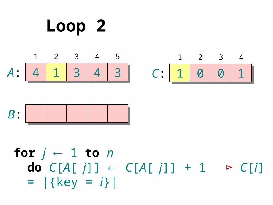
for j 1 to ndo C[A[ j]] C[A[ j]] + 1 ⊳ C[i] = |{key = i}|
Loop 2
A: 4 1 3 4 3
B:
1 2 3 4 5
C: 1 0 0 1
1 2 3 4
for j 1 to ndo C[A[ j]] C[A[ j]] + 1 ⊳ C[i] = |{key = i}|

Loop 2
A: 4 1 3 4 3
B:
1 2 3 4 5
C: 1 0 1 1
1 2 3 4
for j 1 to ndo C[A[ j]] C[A[ j]] + 1 ⊳ C[i] = |{key = i}|

Loop 2
A: 4 1 3 4 3
B:
1 2 3 4 5
C: 1 0 1 2
1 2 3 4
for j 1 to ndo C[A[ j]] C[A[ j]] + 1 ⊳ C[i] = |{key = i}|

Loop 2
A: 4 1 3 4 3
B:
1 2 3 4 5
C: 1 0 2 2
1 2 3 4
for j 1 to ndo C[A[ j]] C[A[ j]] + 1 ⊳ C[i] = |{key = i}|

Loop 3
A: 4 1 3 4 3
B:
1 2 3 4 5
C: 1 0 2 2
1 2 3 4
C': 1 1 2 2
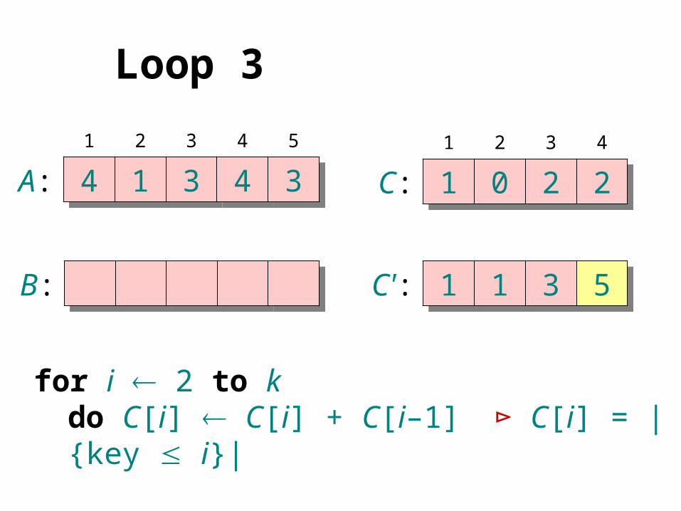
for i 2 to kdo C[i] C[i] + C[i–1] ⊳ C[i] = |{key i}|

Loop 3
A: 4 1 3 4 3
B:
1 2 3 4 5
C: 1 0 2 2
1 2 3 4
C': 1 1 3 2
for i 2 to kdo C[i] C[i] + C[i–1] ⊳ C[i] = |{key i}|
Loop 3
A: 4 1 3 4 3
B:
1 2 3 4 5
C: 1 0 2 2
1 2 3 4
C': 1 1 3 5
for i 2 to kdo C[i] C[i] + C[i–1] ⊳ C[i] = |{key i}|

Loop 4
A: 4 1 3 4 3
B: 3
1 2 3 4 5
C: 1 1 3 5
1 2 3 4
C': 1 1 2 5
for j n downto 1do B[C[A[ j]]] A[ j]
C[A[ j]] C[A[ j]] – 1

Loop 4
A: 4 1 3 4 3
B: 3 4
1 2 3 4 5
C: 1 1 2 5
1 2 3 4
C': 1 1 2 4
for j n downto 1do B[C[A[ j]]] A[ j]
C[A[ j]] C[A[ j]] – 1

Loop 4
A: 4 1 3 4 3
B: 3 3 4
1 2 3 4 5
C: 1 1 2 4
1 2 3 4
C': 1 1 1 4
for j n downto 1do B[C[A[ j]]] A[ j]
C[A[ j]] C[A[ j]] – 1

Loop 4
A: 4 1 3 4 3
B: 1 3 3 4
1 2 3 4 5
C: 1 1 1 4
1 2 3 4
C': 0 1 1 4
for j n downto 1do B[C[A[ j]]] A[ j]
C[A[ j]] C[A[ j]] – 1

Loop 4
A: 4 1 3 4 3
B: 1 3 3 4 4
1 2 3 4 5
C: 0 1 1 4
1 2 3 4
C': 0 1 1 3
for j n downto 1do B[C[A[ j]]] A[ j]
C[A[ j]] C[A[ j]] – 1

Analysisfor i 1 to k
do C[i] 0
(n)
(k)
(n)
(k)
for j 1 to ndo C[A[ j]] C[A[ j]] + 1
for i 2 to kdo C[i] C[i] + C[i–1]
for j n downto 1do B[C[A[ j]]] A[ j]
C[A[ j]] C[A[ j]] – 1(n + k)
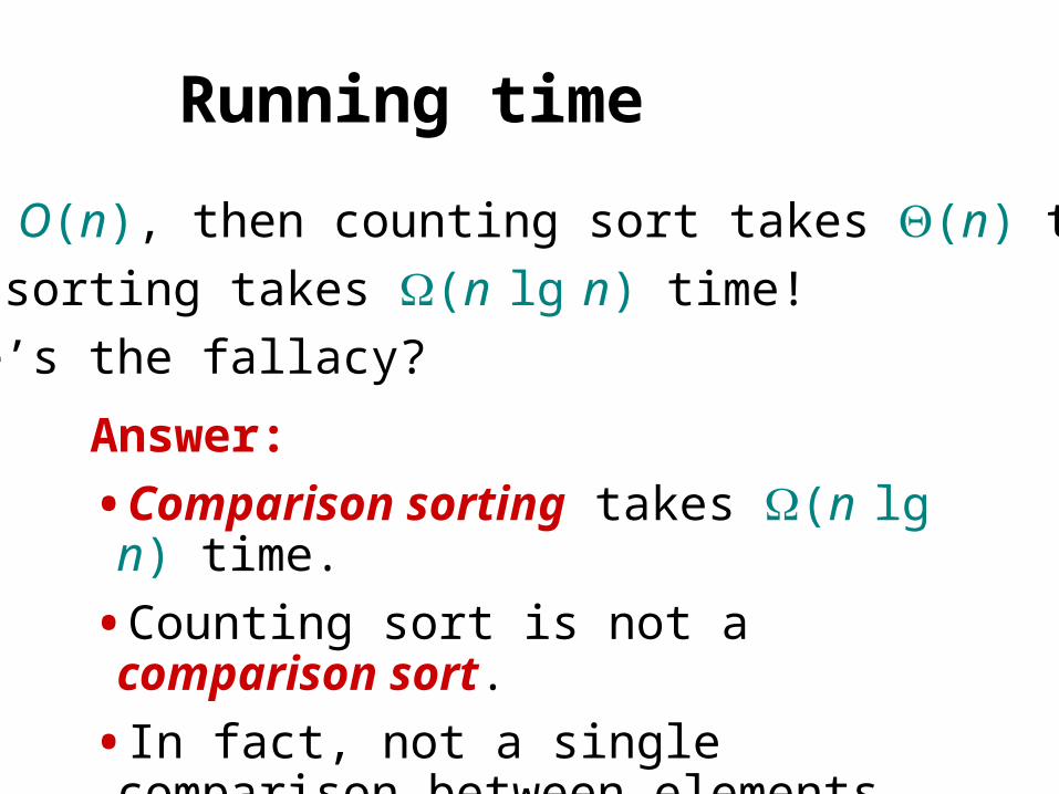
Running time
If k = O(n), then counting sort takes (n) time.
•But, sorting takes (n lg n) time!
•Where’s the fallacy?
Answer:
•Comparison sorting takes (n lg n) time.
•Counting sort is not a comparison sort.
• In fact, not a single comparison between elements occurs!

Stable sorting
Counting sort is a stable sort: it preserves the input order among equal elements.
A: 4 1 3 4 3
B: 1 3 3 4 4
Exercise: What other sorts have this property?

Radix sort
•Origin: Herman Hollerith’s card-sorting machine for the 1890 U.S. Census. (See Appendix .)
•Digit-by-digit sort.
•Hollerith’s original (bad) idea: sort on most-significant digit first.
•Good idea: Sort on least-significant digit first with auxiliary stable sort.

“Modern” IBM card
So, that’s why text windows have 80 columns!
Produced by the WWW Virtual Punch-Card Server.
•One character per column.

Operation of radix sort
3 2 94 5 76 5 78 3 94 3 67 2 03 5 5
7 2 03 5 54 3 64 5 76 5 73 2 98 3 9
7 2 03 2 94 3 68 3 93 5 54 5 76 5 7
3 2 93 5 54 3 64 5 76 5 77 2 08 3 9
•Sort on digit t
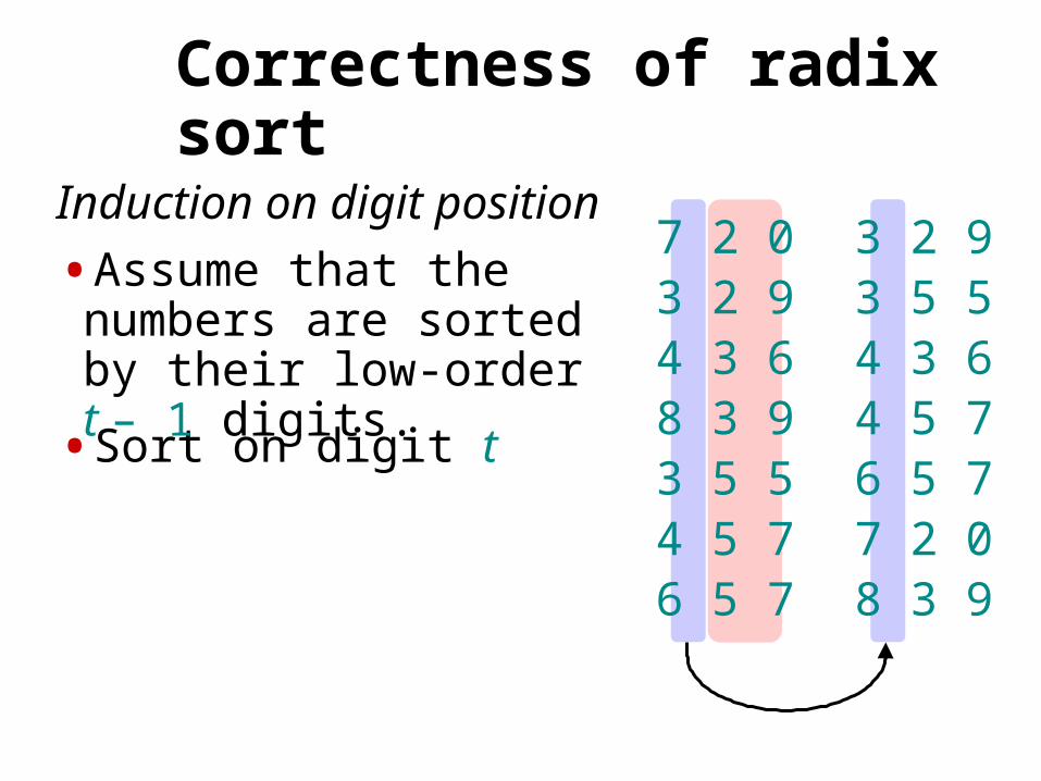
Correctness of radix sort
Induction on digit position
•Assume that the numbers are sorted by their low-order t – 1 digits.
7 2 03 2 94 3 68 3 93 5 54 5 76 5 7
3 2 93 5 54 3 64 5 76 5 77 2 08 3 9

•Sort on digit t
Correctness of radix sort
Induction on digit position
•Assume that the numbers are sorted by their low-order t – 1 digits.
7 2 03 2 94 3 68 3 93 5 54 5 76 5 7
3 2 93 5 54 3 64 5 76 5 77 2 08 3 9
Two numbers that differ in digit t are correctly sorted.

•Sort on digit t
Correctness of radix sort
Induction on digit position
•Assume that the numbers are sorted by their low-order t – 1 digits.
7 2 03 2 94 3 68 3 93 5 54 5 76 5 7
3 2 93 5 54 3 64 5 76 5 77 2 08 3 9
Two numbers that differ in digit t are correctly sorted.
Two numbers equal in digit t are put in the same order as the input correct order.

Analysis of radix sort
•Assume counting sort is the auxiliary stable sort.
•Sort n computer words of b bits each.
•Each word can be viewed as having b/r base-2r digits.Example: 32-bit word
8 8 8 8
r = 8 b/r = 4 passes of counting sort on base-28 digits; or r = 16 b/r = 2 passes of counting sort on base-216 digits.
How many passes should we make?

Analysis (continued)
Recall: Counting sort takes (n + k) time to sort n numbers in the range from 0 to k – 1.If each b-bit word is broken into r-bit pieces, each pass of counting sort takes (n + 2r) time. Since there are b/r passes, we have
.
Choose r to minimize T(n, b):• Increasing r means fewer passes, but as
r > lg n, the time grows exponentially.>

Choosing r??=Minimize T(n, b) by differentiating and setting to 0.
Or, just observe that we don’t want 2r > n, and there’s no harm asymptotically in choosing r as large as possible subject to this constraint.
>
Choosing r = lg n implies T(n, b) = (b n/lg n) .
•For numbers in the range from 0 to n d – 1, we
have b = d lg n radix sort runs in (d n) time.

Conclusions
Example (32-bit numbers):•At most 3 passes when sorting 2000
numbers.•Merge sort and quicksort do at least lg 2000 =
11 passes.
In practice, radix sort is fast for large inputs, as well as simple to code and maintain.
Downside: Can’t sort in place using counting sort. Also, Unlike quicksort, radix sort displays little locality of reference, and thus a well-tuned quicksort fares better sometimes on modern processors, with steep memory hierarchies.

Appendix: Punched-card technology
•Herman Hollerith (1860-1929)
•Punched cards
•Hollerith’s tabulating system
•Operation of the sorter
•Origin of radix sort
•“Modern” IBM card
•Web resources on punched-card technology
Return to last slide viewed.

Herman Hollerith(1860-1929)
•The 1880 U.S. Census took almost10 years to process.
•While a lecturer at MIT, Hollerith prototyped punched-card technology.
•His machines, including a “card sorter,” allowed the 1890 census total to be reported in 6 weeks.
•He founded the Tabulating Machine Company in 1911, which merged with other companies in 1924 to form International Business Machines.

Punched cards
•Punched card = data record.•Hole = value. •Algorithm = machine + human operator.
Replica of punch card from the 1900 U.S. census. [Howells 2000]

Hollerith’s tabulating system•Pantograph card punch
•Hand-press reader
•Dial counters
•Sorting box
Figure from [Howells 2000].

Origin of radix sort
Hollerith’s original 1889 patent alludes to a most-significant-digit-first radix sort:
“The most complicated combinations can readily be counted with comparatively few counters or relays by first assorting the cards according to the first items entering into the combinations, then reassorting each group according to the second item entering into the combination, and so on, and finally counting on a few counters the last item of the combination for each group of cards.”
Least-significant-digit-first radix sort seems to be a folk invention originated by machine operators.

Web resources on punched-card technology
•Doug Jones’s punched card index•Biography of Herman Hollerith•The 1890 U.S. Census•Early history of IBM•Pictures of Hollerith’s inventions•Hollerith’s patent application (borrowed
from Gordon Bell’s CyberMuseum)•Impact of punched cards on U.S. history

Operation of the sorter
• An operator inserts a card into the press.
• Pins on the press reach through the punched holes to make electrical contact with mercury-filled cups beneath the card.
• Whenever a particular digit value is punched, the lid of the corresponding sorting bin lifts.
• The operator deposits the card into the bin and closes the lid.
• When all cards have been processed, the front panel is opened, and the cards are collected in order, yielding one pass of a stable sort.
Hollerith Tabulator, Pantograph, Press, and Sorter


![CS 370: OPERATING SYSTEMS [INTER ROCESS ...SLIDES CREATED BY: SHRIDEEP PALLICKARA L5.1 CS370: Operating Systems [Fall 2018]Dept. Of Computer Science, Colorado State University CS370:](https://img.pdfslide.net/doc/110x75/5fe74a725b8bb82502298942/cs-370-operating-systems-inter-rocess-slides-created-by-shrideep-pallickara.jpg)