Embed Size (px)
Citation preview
Journal of Scheduling 8: 387–426, 2005.© 2005 Springer Science + Business Media, Inc. Manufactured in The Netherlands.
SEQUENCING AND SCHEDULING IN ROBOTIC CELLS:RECENT DEVELOPMENTS
MILIND DAWANDE1, H. NEIL GEISMAR2, SURESH P. SETHI1, ANDCHELLIAH SRISKANDARAJAH1
1University of Texas at Dallas, School of Management, P.O. Box 830688 SM 30, Richardson, TX 75083-0688, USA2College of Business, Prairie View A & M University, P.O. Box 519, Prairie View, TX 77446-0519
ABSTRACT
A great deal of work has been done to analyze the problem of robot move sequencing and part schedulingin robotic flowshop cells. We examine the recent developments in this literature. A robotic flowshop cellconsists of a number of processing stages served by one or more robots. Each stage has one or more machinesthat perform that stage’s processing. Types of robotic cells are differentiated from one another by certaincharacteristics, including robot type, robot travel-time, number of robots, types of parts processed, and useof parallel machines within stages. We focus on cyclic production of parts. A cycle is specified by a repeatablesequence of robot moves designed to transfer a set of parts between the machines for their processing.
We start by providing a classification scheme for robotic cell scheduling problems that is based on threecharacteristics: machine environment, processing restrictions, and objective function, and discuss the influenceof these characteristics on the methods of analysis employed. In addition to reporting recent results onclassical robotic cell scheduling problems, we include results on robotic cells with advanced features such asdual gripper robots, parallel machines, and multiple robots. Next, we examine implementation issues thathave been addressed in the practice-oriented literature and detail the optimal policies to use under variouscombinations of conditions. We conclude by describing some important open problems in the field.
KEY WORDS: manufacturing, robotic cell, cyclic solutions, flexible manufacturing
1. INTRODUCTION
Modern manufacturing processes have incorporated automation and repetitive processing. Em-ploying their efficiency is necessary to compete in the marketplace. Many industries use computer-controlled material handling systems to convey raw materials through the multiple processingstages required to produce a finished product or part. In order to use such systems in a mannerthat provides maximum return on investment, efficient sequences of actions and schedules of partsmust be found.
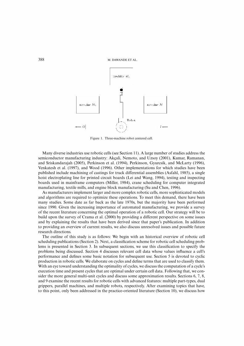
This study focuses on sequencing and scheduling for a particular type of automated materialhandling system in cellular manufacturing: robotic cells. Robotic cells consist of an input device,a series of processing stages, each of which performs a different process on each part in a fixedsequence, an output device, and robots that transport the parts within the cell. (Unless otherwisenoted, all cells considered herein have one robot.) Each stage has one or more machines thatperform that stage’s processing. In essence, a robotic cell is a flowshop with blocking (Pinedo, 1995)that has common servers which perform all transfers of materials between processing stations. SeeFigure 1.
Correspondence to: M. Dawande, E-mail: [email protected]
388 M. DAWANDE ET AL.
Figure 1. Three-machine robot centered cell.
Many diverse industries use robotic cells (see Section 11). A large number of studies address thesemiconductor manufacturing industry: Akcali, Nemoto, and Uzsoy (2001), Kumar, Ramanan,and Sriskandarajah (2005), Perkinson et al. (1994), Perkinson, Gyurcsik, and McLarty (1996),Venkatesh et al. (1997), and Wood (1996). Other implementations for which studies have beenpublished include machining of castings for truck differential assemblies (Asfahl, 1985), a singlehoist electroplating line for printed circuit boards (Lei and Wang, 1994), testing and inspectingboards used in mainframe computers (Miller, 1984), crane scheduling for computer integratedmanufacturing, textile mills, and engine block manufacturing (Su and Chen, 1996).
As manufacturers implement larger and more complex robotic cells, more sophisticated modelsand algorithms are required to optimize these operations. To meet this demand, there have beenmany studies. Some date as far back as the late 1970s, but the majority have been performedsince 1990. Given the increasing importance of automated manufacturing, we provide a surveyof the recent literature concerning the optimal operation of a robotic cell. Our strategy will be tobuild upon the survey of Crama et al. (2000) by providing a different perspective on some issuesand by explaining the results that have been derived since that paper’s publication. In additionto providing an overview of current results, we also discuss unresolved issues and possible futureresearch directions.
The outline of this study is as follows: We begin with an historical overview of robotic cellscheduling publications (Section 2). Next, a classification scheme for robotic cell scheduling prob-lems is presented in Section 3. In subsequent sections, we use this classification to specify theproblems being discussed. Section 4 discusses relevant cell data whose values influence a cell’sperformance and defines some basic notation for subsequent use. Section 5 is devoted to cyclicproduction in robotic cells. We elaborate on cycles and define terms that are used to classify them.With an eye toward understanding the optimality of cycles, we discuss the computation of a cycle’sexecution time and present cycles that are optimal under certain cell data. Following that, we con-sider the more general multi-unit cycles and discuss some approximation results. Sections 6, 7, 8,and 9 examine the recent results for robotic cells with advanced features: multiple part-types, dualgrippers, parallel machines, and multiple robots, respectively. After examining topics that have,to this point, only been addressed in the practice-oriented literature (Section 10), we discuss how
SEQUENCING AND SCHEDULING IN ROBOTIC CELLS: RECENT DEVELOPMENTS 389
robotic cells are used in practice (Section 11). Section 12 outlines some of the fundamental openproblems for future study. We conclude in Section 13.
2. HISTORICAL OVERVIEW
In one of the early papers in the field for robotic cell sequencing, Bedini, Lisini, and Sterpos (1979)develop heuristic procedures for optimizing the working cycle of an industrial robot equippedwith two independent arms. Baumann et al. (1981) derive models to determine robot and machineutilization. Maimon and Nof (1985) and Nof and Hannah (1989) study cells with multiple robots.Devedzic (1990) proposes a knowledge-based system to control the robot.
Wilhelm (1987) classifies the computational complexity of various scheduling problems inassembly cells. In a later study, Hall and Sriskandarajah (1996) survey scheduling problems withblocking and no-wait conditions and classify their computational complexities.
Early studies use simulation to compute cycle times. Kondoleon (1979) uses computer modelingto simulate robot motions in order to analyze the effects of configurations on the cycle time.Claybourne (1983) performs a simulation to study the effects that sequencing robot activitieshas on throughput. Asfahl (1985) simulates the actions of a robotic cell with three machines todemonstrate the transition from cold start to steady state cyclic operations. B�lazewicz, Sethi, andSriskandarajah (1989) develop an analytical method to derive cycle time formulas for robotic cells.Dixon and Hill (1990) compute cycle times by using a database language to simulate robotic cells.
Sethi et al. (1992) set the agenda for most subsequent studies on cells. They provide analyticalsolutions to the robot sequencing problem for two-machine and three-machine cells that produceidentical parts, and for two-machine cells that produce different parts. Logendran and Sriskan-darajah (1996) generalize this work to cells with different types of robots and with more generalrobot travel-times. Brauner and Finke (1997, 1999, 2001a, 2001b) perform several studies thatcompare 1-unit cycles with multi-unit cycles. Crama and van de Klundert (1997a) develop a poly-nomial algorithm for finding an optimal 1-unit cycle in an additive travel-time cell (travel-timesare defined in Section 3.2.2). Dawande, Sriskandarajah, and Sethi (2002) do the same for constanttravel-time cells. Brauner, Finke, and Kubiak (2003) prove that finding the optimal robot movesequence in a robotic cell with general travel-times, called a Euclidean robotic cell, is NP-hard.Hall, Kamoun, and Sriskandarajah (1997, 1998) and Sriskandarajah, Hall, and Kamoun (1998)study part scheduling problems and their complexities for cells that process parts of different types.
Research on cells with no-wait or interval pickup has been performed in parallel with the above-mentioned studies on free-pickup cells (see Section 3.2.1 for information on pickup characteristics).Levner, Kats, and Levit (1997) develop an algorithm that finds an optimal 1-unit cycle in a no-waitcell that produces identical parts. Agnetis (2000) finds optimal part schedules for no-wait cells withtwo or three machines. Agnetis and Pacciarelli (2000) study the complexity of the part schedulingproblem for three-machine cells. Che, Chu, and Levner (2003) present a polynomial algorithm tofind an optimal two-unit cycle in no-wait cells that produce identical parts or two part-types. Katsand Levner (2002) address no-wait cells with multiple robots.
An early work on interval robotic cells is by Lei and Wang (1994), who use a branch andbound search process. Chen, Chu, and Proth (1998) use branch and bound, linear programming,and bi-valued graphs to find optimal 1-unit cycles, and Che, Chu, and Chu (2002) employ thesetechniques to find optimal multi-unit cycles. Kats, Levner, and Meyzin (1999) solve this problemusing a method similar to that used by Levner, Kats, and Levit (1997) for no-wait cells. Complexity
390 M. DAWANDE ET AL.
results for such a system are presented in Crama (1997), Crama and van de Klundert (1997b), andvan de Klundert (1996).
3. A CLASSIFICATION SCHEME
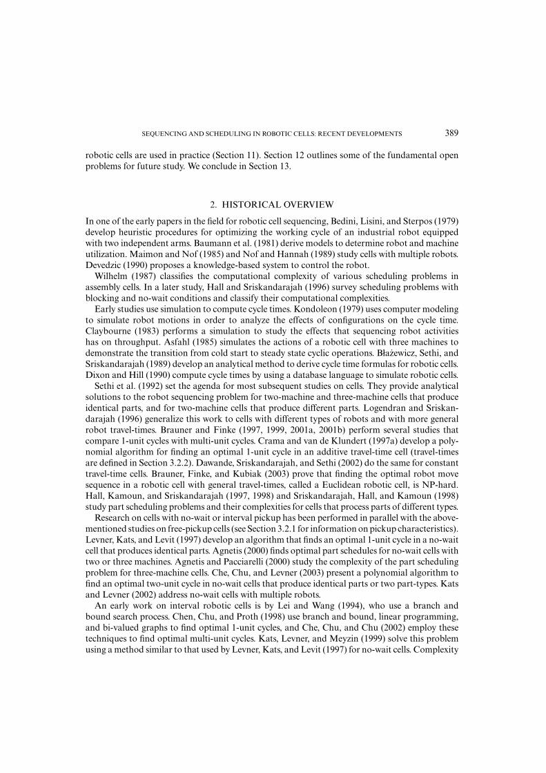
We now present a classification scheme for robotic cell scheduling problems. As in the classificationscheme for classical scheduling problems (Graham et al., 1979), we distinguish problems basedon three characteristics: machine environment (α), processing characteristics (β), and objectivefunction (γ ). A problem is then represented by the form α|β|γ . Following the discussion of thesecharacteristics, we detail our classification in Section 3.4 and also provide a pictorial representationin Figure 2.
Figure 2. A classification for robotic flowshops.

SEQUENCING AND SCHEDULING IN ROBOTIC CELLS: RECENT DEVELOPMENTS 391
3.1. Machine environment
We now describe characteristics that are represented in the first field of our classification scheme.
3.1.1. Number of machines per stageIf each processing stage has only one machine, the robotic cell is called a simple robotic cell or
a robotic flowshop. Such cells contrast with robotic cells with parallel machines, in which at leastone processing stage has more than one machine. Cells with parallel machines are discussed inSection 8.
A typical simple robotic cell contains m processing machines: M1, M2, . . . , Mm. Let M ={1, 2, . . . , m} be the set of indices of these machines. The robot obtains a part from the inputdevice (I, often denoted M0), carries the part to the first machine (M1), and loads the part. AfterM1 completes its processing on the part, the robot unloads the part from M1 and transports it toM2, upon which it loads the part. This pattern continues for machines M3, M4, . . . , Mm, where mrepresents the number of machines in the cell. After Mm has completed its processing on the part,the robot unloads the part and carries it to the output device (O, often denoted Mm+1). In someimplementations, the input device and the output device are at the same location, and this unit iscalled a load lock. A three-machine simple robotic cell is depicted in Figure 1.
This description should not be misconstrued as implying that the robot remains with each partthroughout its processing by each machine. Often, after loading a part onto a machine, the robotmoves to another machine or to the input device in order to collect another part to transport it toits next destination. Determining which sequence of such moves is the optimal has been the focusof the majority of research on robotic cell sequencing and scheduling.
3.1.2. Number of robotsManufacturers employ additional robots in a cell in order to increase throughput by increasing
the material handling capacity. Cells with one (resp. more than one) robot are called single (resp.multiple) robot cells. Most studies in the literature analyze single robot cells. Multiple robot cellsare discussed in Section 9.
3.1.3. Type of robotA single gripper robot can hold only one part at a time. In contrast, dual gripper robots can
hold two parts simultaneously. In a typical usage of this capability, the robot holds one part whilethe other gripper is empty; the empty gripper unloads a machine, the robot repositions the secondgripper, and it loads that machine. Dual gripper robots are discussed in Section 7.
3.2. Processing characteristics
Four different processing characteristics are specified in the second field. We describe three inthis section. The fourth, production strategy, is detailed in Section 3.4.
3.2.1. Pickup criterionA significant feature of the robotic cells that we study is that they have no buffers for intermediate
storage. All parts must be either in the input device, on one of the machines, in the output device,or on the robot.
Robotic cells can be partitioned into three types—free-pickup, no-wait, interval—based on thepickup criterion. Crama et al. (2000) refer to these three types as unbounded processing windows,
392 M. DAWANDE ET AL.
zero-width processing windows, processing windows, respectively. For all three types, a part that hascompleted processing on Mi cannot be loaded onto Mi+1 for its next processing unless Mi+1 isunoccupied, i = 0, . . . , m. In free-pickup cells, this is the only pickup restriction: a completed partmay remain on Mi indefinitely.
For the more restrictive no-wait cells, a part must be removed from machine Mi , i ∈ M, andtransferred to machine Mi+1 as soon as Mi completes processing that part. Such conditions arecommonly seen in steel manufacturing or plastic molding, where the raw material must maintaina certain temperature, or in food canning to ensure freshness (Hall and Sriskandarajah, 1996).Results for no-wait cells can be found in Agnetis (2000), Agnetis and Pacciarelli (2000), Che, Chu,and Levner (2003), Hall and Sriskandarajah (1996), Kats and Levner (2002), and Levner, Kats,and Levit (1997).
In interval robotic cells, each stage has a specific interval of time—a processing time window—for which a part can be processed on that stage. This is applicable, for example, for the HoistScheduling Problem on an electroplating line (Che, Chu, and Chu, 2002; Chen, Chu, and Proth,1998; Lei and Wang, 1994). Printed circuit boards are placed in a series of tanks with differentsolvents. Each tank has a specific interval of time—a processing window—for which a card canremain immersed.
Unless otherwise specified, all cells discussed herein have the free-pickup criterion.
3.2.2. Travel-time metricThe robot’s travel-time between machines greatly influences a cell’s performance. One common
model often applies when the machines are arranged in numeric order in a line or semicircle.The robot’s travel-time between adjacent machines Mi−1 and Mi , denoted d(Mi−1, Mi ), equals δ,for i = 1, . . . , m + 1, and is additive. Additive means that, for the travel-time between any twomachines Mi , Mj , 0 ≤ i, j ≤ m + 1, d(Mi , Mj ) = |i − j |δ (this restriction is also known as thetriangle equality: if i < k < j , then d(Mi , Mj ) = d(Mi , Mk) + d(Mk, Mj ) (Crama et al., 2000)).This scheme is easily generalized to the case of non-equal travel-times between adjacent machines(Brauner and Finke, 1999): d(Mi−1, Mi ) = δi , i = 1, . . . , m + 1, and d(Mi , Mj ) = ∑ j
k=i+1 δk, fori < j . If d(Mi−1, Mi ) = δ, i = 1, . . . , m + 1, then we call the travel-time metric regular additive. Ifd(Mi−1, Mi ) = δi , i = 1, . . . , m + 1, then the cell has general additive travel-times.
There are also additive travel-time cells in which the machines are arranged in a circle so that Iand O are adjacent or in the same location (Drobouchevitch, Sethi, and Sriskandarajah, to appear;Geismar et al., 2004c; Sriskandarajah et al., 2004; Sethi, Sidney, and Sriskandarajah, 2001). Inthese cells, the robot may travel in either direction to move from one machine to another, e.g., tomove from M1 to Mm−1, it may be faster to go via I, O, and Mm, than to go via M2, M3, . . . , Mm−2.For circular cells with regular additive travel-time, d(Mi , Mj ) = min{|i − j |δ, (m+2−|i − j |)δ}. Forgeneral additive travel-time cells, d(Mi , Mj ) = min{∑ j
k=i+1 δk,∑i
k=1 δk + δ0,m+1 + ∑m+1k= j+1 δk}, for
i < j . Throughout the rest of this paper, the additive travel-time metric used will correspond to thatused in the study being cited. Most studies assume that travel-times are symmetric d(Mi , Mj ) =d(Mj , Mi ), 0 ≤ i, j ≤ m + 1, and that the travel-time between two machines does not depend onwhether or not the robot is carrying a part.
To make this model better represent reality, Logendran and Sriskandarajah (1996) enhance it toaccount for the robot’s acceleration and deceleration. The travel-times between adjacent machinesdo not change. However, the travel-time between non-adjacent machines is reduced. For eachintervening machine, the robot is assumed to save η units of time. Therefore, for 0 ≤ i, j ≤ m + 1,
SEQUENCING AND SCHEDULING IN ROBOTIC CELLS: RECENT DEVELOPMENTS 393
if d(Mi−1, Mi ) = δi , then
d(Mi , Mj ) =max(i, j )∑
k=min(i, j )+1
δk − (|i − j | − 1)η.
In Sections 6.2 and 10.1, we present formulas with η because this scheme is used by the studiescited.
For certain cells, additive travel-times are not appropriate. Dawande, Sriskandarajah, and Sethi(2002) discuss a type of cell for which the robot travel-time between any pair of machines is aconstant δ, i.e., d(Mi , Mj ) = δ, 0 ≤ i, j ≤ m +1, i �= j . This arises because these cells are compactand their robots move with varying acceleration and deceleration.
The most general model, one that can most accurately represent any robotic cell, assigns a valueδi j for the robot travel-times between any two machines Mi and Mj , 0 ≤ i, j ≤ m+1. These travel-times are, in general, neither additive nor constant. Brauner, Finke, and Kubiak (2003) address thisproblem by making three rudimentary assumptions that conform to basic properties of Euclideanspace:
1. The travel-time from a machine to itself is zero, i.e., δi i = 0, ∀i .2. The travel-times satisfy the triangle inequality, i.e., δi j + δ jk ≥ δik, ∀i, j, k.3. The travel-times are symmetric, i.e., δi j = δ j i , ∀i, j .
A robotic cell that satisfies Assumptions 1 and 2 is called a Euclidean robotic cell; one that satisfiesAssumptions 1, 2, and 3 is called a Euclidean symmetric robotic cell. The robot move sequencingproblem for either case is NP-hard in the strong sense (Brauner, Finke, and Kubiak, 2003) (seeGarey and Johnson (1979) for a description of computational complexity). This result parallelsone for the Euclidean traveling salesman problem (Lawler et al., 1985). This is also why moststudies approximate reality with additive or constant travel-time models, depending on which ofthe two fits better.
To summarize, three different robot travel-time metrics have been addressed in the literature:additive, constant, and Euclidean. Each study assumes one of these before deriving its results.Therefore, many results in the field have been proven only for one travel-time metric, rather thanfor all three.
3.2.3. Number of part-typesIf the robotic cell produces identical parts, we refer to it as a single part-type cell. In contrast,
multiple part-type cells process lots that contain different types of parts. Generally, these differenttypes have different processing times for a given machine. Multiple part-type cells are discussed inSection 6. Throughout the rest of the paper, unless otherwise specified, the cell under considerationprocesses identical parts.
3.3. Objective function
From an optimization point of view, the only objective addressed in the literature is that ofmaximizing the throughput—the long-term average number of completed parts placed into theoutput buffer per unit time. A precise definition of the throughput is provided in Section 5.
394 M. DAWANDE ET AL.
3.4. An α|β|γ classification for robotic cells
Figure 2 is a pictorial representation of the classification discussed above. A problem is repre-sented using the form α|β|γ , where
(a) α = RF gm,r (m1, . . . , mm). Here, RF stands for “Robotic Flowshop,” m is the number of pro-
cessing stages, and the vector (m1, m2, . . . , mm) indicates the number of machines at eachstage. When this vector is not specified, mi = 1, i = 1, . . . , m, and the cell is a simple cell.The second subscript r denotes the number of robots; when not specified, r = 1. The super-script g denotes the type of robot used. For example, g = 1 (resp. g = 2) denotes a singlegripper (resp. dual gripper) cell. If g is not specified, then g = 1.
(b) β = (pickup, travel-metric, part-type, prod-strategy) where• pickup ∈ {free, no-wait, interval} specifies the pickup criterion.• travel-metric ∈ {A, C, E} specifies the travel-time metric. “A” (resp. “C” and “E”) denotes
the additive (resp. constant and Euclidean) travel-time metric.• If part-type is not specified, the cell produces a single part-type; otherwise part-type = MP
denotes a cell producing multiple part-types.• prod-strategy ∈ {cyclic-k, all, CRM} denotes the specific production strategy employed.
The detailed descriptions of these strategies appear in later sections so we limit our de-scription here and refer the reader to the corresponding section.(i) In a cell producing either a single part-type or multiple part-types, cyclic-k refers to a
cyclic production strategy wherein exactly k units are produced per cycle (Section 5).(ii) In a cell producing either a single part-type or multiple part-types, all refers to a
production environment where all production strategies (i.e., cyclic as well as noncyclic)are considered (Sections 5 and 12).
(iii) In robotic cells producing multiple part-types (Section 6), CRM refers to the concate-nated robot-move sequence strategy (Section 6.1).
(c) γ = µ denotes that the objective function to be addressed is that of maximizing the through-put.
We now illustrate our classification with a few examples.
1. RF4|( free, A, cyclic-1)|µ represents a 4-machine simple robotic cell with one single grip-per robot, a free-pickup criterion, and additive travel-time metric. It produces a singlepart-type and operates a cyclic production strategy wherein one unit is produced per cy-cle. The objective function addressed is maximizing the throughput.
2. RF5(1, 4, 2, 3, 2)|(no-wait, E, cyclic-2)|µ addresses the problem of maximizing throughputfor a 5-stage robotic cell with parallel machines that has 1, 4, 2, 3, and 2 machines, respectively,in stages 1, 2, 3, 4 and 5. The cell produces a single part-type, has one single gripper robot,employs a no-wait pickup criterion and a Euclidean travel-time metric, and produces twounits per cycle.
3. RF2m,3|(interval, C, MP, CRM)|µ considers throughput maximization in an m-machine sim-
ple robotic cell with three dual gripper robots, an interval pickup criterion, constant travel-time metric, and multiple part-type production using a CRM production strategy.
In the following sections, we use this classification to specify the problem being discussed.
SEQUENCING AND SCHEDULING IN ROBOTIC CELLS: RECENT DEVELOPMENTS 395
4. CELL DATA
In addition to the robot’s travel-time metric, each stage’s processing time and the times requiredfor loading and unloading a machine influence the cell’s throughput. We now discuss these char-acteristics and the notation for representing the cell’s actions and states. First, we list the basicassumptions throughout most studies:
� All data and events are deterministic.� All processing is nonpreemptive.� Parts to be processed are always available at the cell’s input device.� There is always space for completed parts at the output device.� All data are rational.
4.1. Processing times
Since each of the m stages performs a different function, each, in general, has a different pro-cessing time for a given part. For cells with free-pickup or no-wait pickup, the processing timeof a machine in stage i is denoted by pi , i ∈ M. If a cell processes k different types of parts, theprocessing time of part j on stage i is denoted by pi j , i ∈ M; j = 1, . . . , k. In interval robotic cells,the processing time of machine Mi is specified by a lower bound ai and an upper bound bi , e.g.,the time that a printed circuit board spends in tank i must be in the interval [ai , bi ]. If multiplepart-types are processed in an interval robotic cell, the processing interval for part-type j is denotedby [ai j , bi j ].
4.2. Loading and unloading times
Another factor that influences the processing duration for a part is the time required for loadingand unloading at each machine. For uniformity, picking a part from I is referred to as unloadingI = M0, and dropping a part at O is referred to as loading O = Mm+1. A common and simplemodel assumes that the loading and unloading times are equal to ε for all machines (Ioachim andSoumis, 1995). More sophisticated models (Brauner and Finke, 2001a) have different values forloads and unloads for each machine: unloading time for Mi is εu
i , i = 0, . . . , m, and loading timefor Mi is εl
i , i = 1, . . . , m + 1.
4.3. Notations for cell states and robot actions
The concept of an activity is widely used in the study of robotic cells. In a simple robotic cell,activity Ai , i = 0, . . . , m, consists of the following sequence:
1. The robot unloads a part from Mi
2. The robot travels from Mi to Mi+1
3. The robot loads this part onto Mi+1.
Since a part must be processed on all m machines and then placed into the output buffer, oneinstance of each of the m + 1 activities A0, A1, . . . , Am is required to produce a part.
A notation that represents the state of the cell is also very useful. Information that it mustconvey includes the status of each machine (occupied or not occupied by a part) and the stateof the robot (location and occupancy). This can be presented as an (m + 1)-dimensional state
396 M. DAWANDE ET AL.
space (e1, . . . , em+1), as shown in Sethi et al. (1992). The first m dimensions each correspond to amachine: ei = φ if Mi is unoccupied; ei = � if Mi is occupied, i ∈ M. The last dimension representsthe robot. em+1 = Ai indicates that the robot has just completed activity Ai , i = 0, . . . , m.
For m = 4, an example state is (�, φ, φ, �, A3) : M2 and M3 are unoccupied, M1 and M4 areoccupied, and the robot has just completed loading M4. From this point, let us now consider whathappens if the robot executes activity sequence A1 A2 A4: the robot moves to M1, waits for M1 tofinish processing (if required), unloads a part from M1, travels to M2, and loads the part onto M2.At this instant, the state of the cell is (φ, �, φ, �, A1). The robot waits at M2 for the entirety ofthe part’s processing. The robot then unloads the part from M2, carries it to M3, and loads thepart onto M3. The cell’s state is now (φ, φ, �, �, A2). The robot next travels to M4, waits for M4
to finish processing (if required), unloads a part from M4, travels to the output buffer, and loadsthe part onto the output buffer, so the cell’s state is (φ, φ, �, φ, A4).
It is important to note that this state description is not a complete definition of the state, as itomits information representing the extent of the processing completed on the parts on the variousmachines. However, as we are mainly concerned about cyclic solutions (defined in Section 5),we see later in Section 5.1.2 that a condition that defines cyclic solutions completes the missinginformation in the state description. Thus, for our purposes, this state description is sufficient.
5. CYCLIC PRODUCTION
Cyclic production in a robotic cell refers to the production of finished parts by repeating a fixedsequence of robot moves. The main motivation for studying cyclic production comes from practice:cyclic schedules are easy to implement and control and are the primary way of specifying theoperation of a robotic cell in industry. In a recent result, Dawande, Geismar, and Sethi (to appear)show that it is sufficient to consider cyclic schedules in order to maximize throughput. That is,there is at least one cyclic schedule in the set of all schedules that optimizes the throughput ofthe cell. The main idea behind this result is easy to explain: a robotic cell can be modeled as afinite state dynamic system. Any potential throughput-maximizing way of operating the cell canbe represented by a policy (function) defined on the finite state space. The finiteness of the statespace then implies that any particular policy repeats a minimal sequence of robot moves and, thus,gives rise to a cyclic schedule.
Using the notation defined in the previous section, cyclic production can be represented as arepeatable sequence of activities. For example, (A0, A2, A4, A3, A1) is a sequence of activities thatproduces a part in a four-machine cell. Such a sequence can be repeated in a cyclic fashion, witheach iteration producing a single part. To formalize, we define the following terms:
Definition. A k-unit activity sequence is a sequence of robot moves which loads and unloadseach machine exactly k times.
To be feasible, an activity sequence must satisfy two criteria:
� The robot cannot be instructed to load an occupied machine� The robot cannot be instructed to unload an unoccupied machine.
These concepts are operationalized as follows: During cyclic operations, for i = 1, . . . , m − 1,between any two occurrences of Ai there must be exactly one Ai−1 and exactly one Ai+1. Thiscondition implies that between any two instances of A0 there is exactly one A1, and betweenany two instances of Am there is exactly one Am−1. For instance, in a cell with m = 3, the 2-unit
SEQUENCING AND SCHEDULING IN ROBOTIC CELLS: RECENT DEVELOPMENTS 397
activity sequence (A0, A1, A3, A1, A2, A0, A3, A2) is infeasible because the second occurrence ofA1 attempts to unload machine M1 when it is empty. Note that all 1-unit activity sequences arefeasible.
Definition. A k-unit cycle is the performance of a feasible k-unit activity sequence in a waywhich leaves the cell in exactly the same state as its state at the beginning of those moves.
For every feasible k-unit activity sequence, k ≥ 1, there is at least one initial state for which it is ak-unit cycle, i.e., if the k-unit activity sequence begins with this state, it leaves the cell in exactly thesame state after its execution (Sriskandarajah et al., 2004). Since a k-unit cycle preserves the stateof the cell, repeating it indefinitely yields a k-unit cyclic solution. A cyclic solution is also knownas a steady state solution. We provide a more rigorous definition of steady state below.
A k-unit activity sequence has k(m + 1) activities, i.e., each of the m + 1 activities is performedexactly k times and in an order that satisfies the feasibility constraints. A k-unit cycle constructedfrom a k-unit activity sequence (A0, Ai1 , Ai2 , . . . , Aik(m+1)−1 ) will be referred to as the k-unit cycle(A0, Ai1 , Ai2 , . . . , Aik(m+1)−1 ) or, simply, cycle (A0, Ai1 , Ai2 , . . . , Aik(m+1)−1 ) . Since a k-unit cyclic solu-tion is completely characterized by a k-unit cycle, we will use the two terms interchangeably whenno confusion arises by doing so.
Define the function S(Ai , t) to represent the time of completion of the tth execution of activityAi (Crama and van de Klundert, 1997a). Given a feasible infinite sequence of activities and acompatible initial state, we can define the long-run average throughput or, simply, throughput to be
µ = limt→∞
tS(Am,t)
.
Intuitively, this quantity represents the long-term average number of completed parts placed intothe output buffer per unit time.
Obtaining a feasible infinite sequence of activities that maximizes throughput is a fundamentalproblem of robotic cell scheduling. Such a sequence of robotic moves is called optimal. Moststudies focus on infinite sequences of activities in which a fixed sequence of m+1, or some integralmultiple of m + 1, activities is repeated cyclically.
Definition (Crama and van de Klundert, 1997a). A robotic cell repeatedly executing a k-unitcycle π of robot moves is operating in steady state if there exists a constant T(π ) and a constant Nsuch that for every Ai , i = 0, . . . , m, and for every t ∈ Z
+ such that t > N, S(Ai , t + k)−S(Ai , t) =T(π ). T(π ) is called the cycle time of π .
For additive travel-time cells, we denote the cycle time by Ta(π ). For constant travel-time cells, wedenote the cycle time by Tc(π ). For Euclidean travel-time cells, we denote the cycle time by Te(π ).
The per unit cycle time of a k-unit cycle π is T(π )k . This is the reciprocal of the throughput
and is easier to calculate directly. Therefore, minimizing the per unit cycle time is equivalent tomaximizing the throughput.
An assumption in most studies is that the sequence of robot moves is active.
Definition. A sequence is called active if the robot always executes the next operation, whateverthat may be, as soon as possible.
For active sequences, all execution times for the robot’s actions are uniquely determined once thesequence of activities is given. The robot’s only possible waiting period can occur at a machine atwhich the robot has arrived to unload, but the machine has not completed processing its current
398 M. DAWANDE ET AL.
part. It is known that there always exists an active sequence that is optimal within the class of1-unit cycles (van de Klundert, 1996).
Brauner and Finke (2001b) show that repeating a k-unit activity sequence will enable the roboticcell to reach a steady state (or cyclic solution) in finite time. Therefore, since we are maximizingthe long-run average throughput, i.e., assuming that the cell operates in steady state for an infinitetime, there is no impact from the initial transient phase (Hall, Kamoun, and Sriskandarajah, 1998;Dawande, Geismar, and Sethi, to appear). Hence, there is no loss of generality by studying only thesteady state behavior. Nevertheless, there may be some practical reason to find the time requiredto reach steady state. This is discussed in Section 10.1.
5.1. Cycle times
In this section we discuss the robot’s waiting time at a particular machine and a method offinding the cycle time of a 1-unit cycle in a simple robotic cell. We also establish lower bounds forthe cycle time.
5.1.1. Waiting timesThe robot waits at a machine Mi if its next sequenced action is to unload Mi , but Mi has not
yet completed processing its current part. The length of the robot’s waiting time, denoted wi , atmachine Mi , i ∈ M, is Mi ’s processing time pi minus the time that elapses between when Mi wasloaded and when the robot returns to unload it. If this difference is negative, then the waiting timeis zero.
The time that elapses between Mi ’s loading and the robot’s return is determined by the inter-vening activities that are executed between the loading and the unloading of Mi . If there are nointervening activities, the robot loads Mi , waits at Mi for time pi , then unloads Mi . Such a sequenceis represented by Ai−1 Ai . In this case, Mi is said to have full waiting (Dawande, Sriskandarajah,and Sethi, 2002).
If there are intervening activities between the loading and the unloading of Mi , then Mi haspartial waiting (Dawande, Sriskandarajah, and Sethi, 2002). Consider the sequence Ai−1 Aj Ai .The robot loads Mi , travels to Mj (δi, j ), waits for Mj to complete processing (w j ), unloads Mj (εu
j ),carries that part to Mj+1 (δ j, j+1), loads Mj+1 (εl
j+1), then travels to Mi (δ j+1,i ). The robot’s waitingtime at Mi is
wi = max{
0, pi − δi, j − w j − εuj − δ j, j+1 − εl
j+1 − δ j+1,i}.
For a constant travel-time cell, this expression simplifies to wi = max{0, pi − 3δ − 2ε − w j }.The expression for the robot’s waiting time is often dependent on the waiting time at another
machine. This recursion makes calculating the cycle time more difficult. However, the conditionthat a cycle begins and ends in the same state allows us to uniquely compute the cycle times, asdemonstrated in the next section.
5.1.2. Computing cycle timesThe cycle time is calculated by summing the robot’s movement times, the loading and unloading
times, and the robot’s waiting times (full and partial). Unlike the linear programming approachused in Crama et al. (2000), we need not directly deduce the exact time at which each machine isloaded and unloaded.
SEQUENCING AND SCHEDULING IN ROBOTIC CELLS: RECENT DEVELOPMENTS 399
For each activity Ai , i = 0, . . . , m, the robot unloads Mi , carries the part to Mi+1, and loadsMi+1. The total time for Ai is εu
i + δi,i+1 + εli+1.
We must also account for the time between activities. If Mi has full waiting (Ai−1 immediatelyprecedes Ai ), the robot spends exactly pi time units between activities Ai−1 and Ai waiting at Mi .If Mi has partial waiting (Aj immediately precedes Ai , j �= i −1), then the robot moves from Mj+1
to Mi (δ j+1,i ) and waits for Mi to complete processing (wi ) before starting activity Ai .For clarity, we now assume a constant travel-time cell with constant loading and unloading
times. Let V1 be the set of machines with full waiting, and V2 be the set of those with partialwaiting. The cycle time for a 1-unit cycle is
Tc(π ) = (m + 1)(δ + 2ε) +∑
i∈V1
pi +∑
i∈V2
(wi + δ) + δ. (1)
The extra δ accounts for the last movement of the cycle, which takes the robot to I to collect a newpart.
For example, consider the cycle S3 = (A0, A1, A3, A2). V1 = {1}, V2 = {2, 3}, m = 3.
Tc(S3) = 4(δ + 2ε) + p1 + w2 + w3 + 3δ
= 7δ + 8ε + p1 + w2 + w3
w2 = max{0, p2 − 3δ − 2ε − w3}w3 = max{0, p3 − 4δ − 4ε − p1}
w2 + w3 = max{0, p2 − 3δ − 2ε, p3 − 4δ − 4ε − p1}Tc(S3) = max{7δ + 8ε + p1, 4δ + 6ε + p1 + p2, 3δ + 4ε + p3}
Similarly, the cycle time for the cycle S6 = (A0, A3, A2, A1) is Tc(S6) = max{8δ + 8ε, p1 + 3δ +4ε, p2 + 3δ + 4ε, p3 + 3δ + 4ε}. Writing the equations for the waiting times requires that thecycle begins and ends in the same state. In general, this method can be implemented as a linearprogram with km variables and km constraints, where k is the number of units produced in onecycle (Geismar, Dawande, and Sriskandarajah, 2004b; Kumar, Ramanan, and Sriskandarajah,2005). Hence, it has complexity O((km)3L), where L is the size of the problem’s binary encoding.
Crama and van de Klundert (1997a) develop an O(m) time algorithm to find the cycle time inan additive travel-time cell of any member of a dominant subset of cycles called pyramidal cycles.Pyramidal cycles are discussed in greater detail in Section 5.2.
There are alternative graphical methods that find cycle times without considering robot waitingtimes. We refer the reader to Crama et al. (2000) for an extensive description of these.
5.1.3. Lower bounds on cycle timesFrom equation (1) we can deduce a lower bound for the cycle time for a 1-unit cycle in a
constant travel-time cell (problem RFm|( free, C, cyclic-1)|µ). Obviously, for any cycle, Tc(π ) ≥2(m + 1)ε + (m + 2)δ. If all machines with partial waiting have wi = 0, then the minimum valuefor Tc(π ) is achieved by minimizing
∑i∈V1
pi + ∑i∈V2
δ, which is done by placing those machinesfor which pi ≤ δ in V1. Thus, in a constant travel-time robotic cell, for any 1-unit cycle π, Tc(π ) ≥(m + 2)δ + ∑m
i=1 min{pi , δ} + 2(m + 1)ε (Dawande, Sriskandarajah, and Sethi, 2002). In a regular

400 M. DAWANDE ET AL.
additive travel-time robotic cell (problem RFm|( free, A, cyclic-1)|µ), for any 1-unit cycle π, Ta(π ) ≥2(m + 1)(δ + ε) + ∑m
i=1 min{pi , δ} (Crama and van de Klundert, 1997a).Suppose that p j = max1≤i≤m pi is large relative to δ and ε. Since the cycle time can be measured
as the time between successive loadings of Mj , we can derive another lower bound for the cycletime of a 1-unit cycle. This includes, at minimum, the times for the following: Mj ’s processing,unload Mj , move to Mj+1, load Mj+1, move to Mj−1, unload Mj−1, move to Mj , load Mj . Forconstant travel-time, this value is p j + 3δ + 4ε; for regular additive travel-time, p j + 4(δ + ε).We combine these bounds, originally derived by Dawande, Sriskandarajah, and Sethi (2002) andCrama and van de Klundert (1997a), respectively, in the following theorem.
Theorem 1. For 1-unit cycles, the following are lower bounds for constant travel-time roboticcells (problem RFm|( free, C, cyclic-1)|µ) and regular additive travel-time robotic cells (problemRFm|( free, A, cyclic-1)|µ), respectively:
Tc(π ) ≥ max
{
(m + 2)δ +m∑
i=1
min{pi , δ} + 2(m + 1)ε, max1≤i≤m
pi + 3δ + 4ε
}
Ta(π ) ≥ max
{
2(m + 1)(δ + ε) +m∑
i=1
min{pi , δ}, max1≤i≤m
pi + 4(δ + ε)
}
.
5.2. Optimal 1-unit cycles
We first examine two elementary cycles on simple robotic cells with free-pickup and then examinespecific conditions under which they are optimal. We then discuss two classes of cycles in whichan optimal cycle can be found under more general conditions for cells with free-pickup, andsummarize an approach to finding optimal cycles for no-wait cells.
5.2.1. Special casesIn the forward cycle πU = (A0, A1, A2, . . . , Am−1, Am), often called S1, the robot unloads a part
from I, carries it to M1, loads M1, waits for M1 to process the part, unloads M1, then carries thepart to M2. The robot continues in this fashion, waiting at each machine for its entire processingof the part. Only one machine is processing a part at any given time. The processing times for πU
in constant and regular additive travel-time robotic cells, respectively, are
Tc(πU) = 2(m + 1)ε +m∑
i=1
pi + (m + 2)δ
Ta(πU) = 2(m + 1)ε +m∑
i=1
pi + 2(m + 1)δ.
For constant and additive travel-time simple robotic cells, Theorems 2–4 below provide an optimal1-unit cycle under specific conditions. In terms of the classification provided in Section 3.4, theseresults are for problems RFm|( free, C, cyclic-1)|µ and RFm|( free, A, cyclic-1)|µ.
Theorem 2. For both constant and regular additive travel-time robotic cells, if pi ≤ δ, ∀i, then πU
achieves the optimal 1-unit cycle time.
SEQUENCING AND SCHEDULING IN ROBOTIC CELLS: RECENT DEVELOPMENTS 401
This result follows immediately from Theorem 1 (Dawande, Sriskandarajah, and Sethi, 2002).The reverse cycle for a simple robotic cell, often called Sm!, is πD = (A0, Am, Am−1, . . . , A2, A1).
To perform πD, the robot unloads a part from the input buffer (M0), carries it to M1, and loadsM1. It then travels to Mm, unloads Mm, and carries that part to the output buffer (Mm+1). It repeatsthis sequence for i = m − 1, m − 2, . . . , 1: travel to Mi , unload Mi , carry the part to Mi+1, loadMi+1. After loading M2 (which completes activity A1), the robot completes the cycle by travelingto the input buffer (M0). At each machine, before unloading a part from it, the robot may have towait for that machine to complete processing.
The cycle times for πD in constant (Dawande, Sriskandarajah, and Sethi, 2002) and regularadditive (Crama and van de Klundert, 1997a) travel-time robotic cells, respectively, are
Tc(πD) = max{
2(m + 1)(δ + ε), max1≤i≤m
pi + 3δ + 4ε}
Ta(πD) = max{
4mδ + 2(m + 1)ε, max1≤i≤m
pi + 4(δ + ε)}
.
Note that in each formula, the first argument represents the cycle time if the robot never waits fora machine to complete its processing.
For each of the following two theorems, if its premises are met, then πD achieves the lower boundstated in Theorem 1. This yields the following theorem from Dawande, Sriskandarajah, and Sethi(2002) and Crama and van de Klundert (1997a):
Theorem 3. In a constant travel-time robotic cell (problem RFm|( free, C, cyclic-1)|µ), ifmax1≤i≤m pi + 3δ + 4ε ≥ 2(m + 1)(δ + ε), then πD is an optimal 1-unit cycle. In a regular ad-ditive travel-time robotic cell (problem RFm|( free, A, cyclic-1)|µ), if max1≤i≤m pi + 4(δ + ε) ≥4mδ + 2(m + 1)ε, then πD is an optimal 1-unit cycle.
Theorem 3 can be generalized to the Euclidean travel-time case (problem RFm|( free,E, cyclic-1)|µ). If
max1≤i≤m
{pi + δi,i+1 + δi+1,i−1 + δi−1,i + 4ε} ≥ 2(m + 1)ε +m∑
i=0
δi,i+1 +m+1∑
i=2
δi,i−2 + δ1,m, (2)
then πD is optimal. If condition (2) holds, then Te(πD) = max1≤i≤m{pi + δi,i+1 +δi+1,i−1 + δi−1,i + 4ε}, which, by following the logic of Section 5.1.3 and using the triangle in-equality, we see is a lower bound on the cycle time.
The following theorem is proven by Dawande, Sriskandarajah, and Sethi (2002).
Theorem 4. For constant travel-time robotic cells (problem RFm|( free, C, cyclic-1)|µ), if pi ≥δ, ∀i , then πD achieves the optimal 1-unit cycle time.
This theorem is not true for additive travel-time robotic cells. Consider the following example:π1 = (A0, A1, Am, Am−1, . . . , A2), with pi ≥ δ, ∀i .
Ta(π1) = max{(4m − 2)δ + 2(m + 1)ε + p1, p2 + p1 + 6(δ + ε), max3≤i≤m
{pi + 4(δ + ε)}} (3)
402 M. DAWANDE ET AL.
If
p2 + p1 + 6(δ + ε) ≤ (4m − 2)δ + 2(m + 1)ε + p1, and
max3≤i≤m
{pi + 4(δ + ε)} ≤ (4m − 2)δ + 2(m + 1)ε + p1,
then Ta(π1) = (4m − 2)δ + 2(m + 1)ε + p1. If p1 < 2δ, then Ta(πD) = 4mδ + 2(m + 1)ε, andTa(π1) < Ta(πD). However, we do have the following results for regular additive travel-time cells.
Theorem 5. For problem RFm|( free, A, cyclic-1)|µ, if
pi + pi+1 ≥ (4m − 6)δ + 2(m − 2)ε, i = 1, . . . , m − 1,
then πD is optimal.
Proof. See the Appendix. �
Corollary 1. For problem RFm|( free, A, cyclic-1)|µ, if
pi ≥ (2m − 3)δ + (m − 2)ε, i = 1, . . . , m,
then πD is optimal.
5.2.2. General casesTo find an optimal 1-unit cycle in additive travel-time cells (problem RFm|( free, A, cyclic-1)|µ),
Crama and van de Klundert (1997a) employ a concept that has been used to analyze travelingsalesman problems: the set of 1-unit pyramidal cycles (Lawler et al., 1985).
Definition. The 1-unit cycle π = (A0, Ai1 , Ai2 , . . . , Aim ) is pyramidal if there exists a k ∈ Msuch that 1 ≤ i1 < i2 < · · · < ik = m, and m > ik+1 > ik+2 > · · · > im ≥ 1. In such a cycle, U ={i1, i2, . . . , ik} is the set of uphill activities and D = {ik+1, ik+2, . . . , im} is the set of downhillactivities.
πU and πD are pyramidal, as is (A0, A2, A5, A7, A6, A4, A3, A1). In an m-machine cell, there are2m−1 pyramidal cycles. Crama and van de Klundert (1997a) show that the set of pyramidal cyclesis dominant over all 1-unit cycles in additive travel-time cells.
Definition. A set of cycles is dominant if, for every choice of the processing times, there existsπ ∈ such that T(π )/kπ ≤ T(π ′)/kπ ′ , ∀π ′ �∈ , where π is a kπ -unit cycle, and π ′ is a kπ ′ -unitcycle.
They also devise a dynamic programming algorithm that finds the optimal pyramidal permutationin O(m 3) time (Crama and van de Klundert, 1997a).
Pyramidal cycles do not dominate the class of 1-unit cycles in constant travel-time cells form ≥ 3 (problem RFm|( free, C, cyclic-1)|µ), but the set of basic cycles does. To create a basic cyclefor a cell, one first must decide which machines Mi have full waiting (i ∈ V1), and which havepartial waiting (i ∈ V2). Each element of the set {Ai : i ∈ V2 ∪ {0}} is the first element of a stringτi = {Ai , Ai+1, . . . , Ai+li }. All other elements of a string correspond to machines with full waiting:both i + k ∈ V1, k = 1, . . . , li , and i + li + 1 ∈ V2 ∪ {m + 1}, for i ∈ V2 ∪ {0}. The basic cycle isformed by concatenating the strings in reverse order (Dawande, Sriskandarajah, and Sethi, 2002).Consider the following example:
SEQUENCING AND SCHEDULING IN ROBOTIC CELLS: RECENT DEVELOPMENTS 403
Example. m = 8, V1 = {1, 2, 4, 8}, and V2 = {3, 5, 6, 7}. There are five strings: τ0 ={A0, A1, A2}, τ3 = {A3, A4}, τ5 = {A5}, τ6 = {A6}, and τ7 = {A7, A8}. The basic 1-unit cycle cor-responding to V1 is (τ0, τ7, τ6, τ5, τ3) = (A0, A1, A2, A7, A8, A6, A5, A3, A4).
In a cell with m machines, there are 2m −m basic cycles. To find the optimal basic cycle, Dawande,Sriskandarajah, and Sethi (2002) devise an O(m 2 log(mδ)) algorithm based on repeatedly solvinga shortest path problem in a directed acyclic network.
For no-wait cells (Levner, Kats, and Levit, 1997), develop a polynomial algorithm for finding theminimum cycle time for Euclidean travel-time cells (problem RFm|(no-wait, E, cyclic-1)|µ). It usesthe machine’s processing times and the robot’s travel-times to derive infeasible intervals for the cycletime. The optimal cycle time is the smallest positive number not in these intervals. Obviously, thisalgorithm can be applied to the less general cases of additive (problem RFm|(no-wait, A, cyclic-1)|µ)and constant (problem RFm|(no-wait, C, cyclic-1)|µ) travel-times, too.
5.3. Quality of 1-unit cycles and approximation results
Having found optimal cycles for problems RFm|( free, A, cyclic-1)|µ and RFm|( free, C,
cyclic-1)|µ, the question naturally arises, “Is the optimal 1-unit cycle superior to every nontrivialk-unit cycle, k ≥ 2?” Sethi et al. (1992) prove this to be true for RF2|( free, A, cyclic-1)|µ and con-jectured it to be so for m ≥ 3. The attraction of this possibility is obvious: 1-unit cycles are theeasiest to understand, analyze, and control. If they also have the highest throughput, there is noreason to consider the more complex and more numerous multiunit cycles.
For RF3|( free, A, cyclic-1)|µ, Crama and van de Klundert (1999) and Brauner and Finke(1999a) each prove that the Sethi et al. conjecture is true. The conjecture does not holdfor RF4|( free, A, cyclic-1)|µ, however. Brauner and Finke (1997, 2001b) provide a counterex-ample. For RF4|( free, C, cyclic-1)|µ, consider the cell with the following data (Dawande,Geismar, and Sethi, to appear): p1 = 22, p2 = 1, p3 = 1, p4 = 22, δ = 4, ε = 0. The best 1-unitcycle is (A0, A4, A3, A1, A2), whose cycle time is 39. The best 2-unit cycle time is achieved by(A0, A4, A3, A1, A0, A4, A2, A3, A1, A2), whose per unit cycle time is 38. Note that althoughthis 2-unit cycle dominates all 1-unit cycles and all 2-unit cycles in this cell, we cannot as-sert its optimality for all k-unit cycles, k ≥ 1. By Theorem 1, the lower bound on the opti-mal value is 34, so there may be a k-unit cycle, k ≥ 3, that has per unit cycle time less than38.
Similar results for RFm|(no-wait, A, cyclic-1)|µand RFm|(interval, A, cyclic-1)|µare summarizedin Crama et al. (2000).
Even though 1-unit cycles do not dominate, their simplicity still makes them attractive in practice.We have seen that the reverse cycle πD is optimal under certain conditions. Crama and van deKlundert (1997a) show that for RFm|( free, A, cyclic-1)|µ, πD is a 2-approximation. Brauner andFinke (2001a) show that if the optimum per unit cycle time over all k-unit cycles is Topt, then onecan guarantee that
Ta(πD) ≤(
2 − δ1 + δm+1
δ1 + δm+1 + ∑mi=2 δi
)
Topt ≤ 2Topt.
404 M. DAWANDE ET AL.
For RFm|( free, C, cyclic-1|µ, we have
Tc(πD) ≤(
2(m + 1)(δ + ε)(m + 2)δ + 2(m + 1)ε
)
Topt ≤(
2(m + 1)δ(m + 2)δ
)
Topt ≤ 2Topt.
The most recent approximation algorithms for 1-unit cycles in additive, constant, and Eu-clidean travel-time cells are by Geismar, Dawande, and Sriskandarajah (2005). For both problemRFm|( free, A, cyclic-1)|µ and problem RFm|( free, C, cyclic-1)|µ, they develop algorithms thatproduce 1-unit cycles whose cycle times are within a factor of 1.5 of the optimum per unit cy-cle time. For Euclidean travel-time cells, where the optimum 1-unit cycle problem (i.e. problemRFm|( free, E, cyclic-1)|µ) is NP-complete (Brauner, Finke, and Kubiak, 2003), they develop analgorithm that produces a 1-unit cycle whose cycle time is within a factor of 1.5q of the optimumper unit cycle time, where
q = max0≤i, j≤m+1{δi j }min0≤i, j≤m+1{δi j } , i �= j.
Should this ratio be large (q ≥ 2.67), it is also shown that πD is a 4-approximation. All threealgorithms run in O(m) time.
An approximation result for dual gripper robot cells (problem RF2m|( free, A, MP, CRM)|µ)
can be found in Section 7. Heuristics for RFm|( free, A, MP, cyclic-k)|µ are described inSection 6.3.
6. MULTIPLE PART-TYPES
We now examine robotic cells that process lots that contain different types of parts. Generally,parts of different types have different processing times for a given machine. Such implementationsare more common in smaller manufacturers. They process multiple parts in a single lot in order tohave enough volume to use the cell efficiently (Ramanan, 2002).
In accordance with just-in-time manufacturing, the relative proportions of the part-types in eachlot should be the same as the relative proportions of the demand. Consequently, researchers focuson cycles which contain the minimal part set (MPS) that has these same proportions. For example,if the demand for a company’s three products is divided so that product A has 40%, product Bhas 35%, and product C has 25%, the MPS has 20 parts: 8 of product A, 7 of product B, and 5 ofproduct C. In practice, the size of an MPS can be larger than 50 parts (Wittrock, 1985).
In general, the cell processes k different part-types. In one MPS, ri parts of type i are produced,i = 1, . . . , k. The total number of finished parts in a cycle is n = r1+· · ·+rk. The schedule accordingto which the parts are produced is specified by a permutation σ . Pσ (i ) is the part scheduled in thei th position of σ, i = 1, . . . , n.
6.1. MPS cycles and CRM sequences
Given an MPS of n parts, an MPS cycle is a sequence of robot moves in which exactly n partsof an MPS enter the cell at I, exactly n parts of an MPS exit the cell at O, and the cell returns to itsinitial state. The order in which the parts enter the cell is called the MPS part schedule (or simplypart schedule). An MPS cycle is determined by the MPS part schedule and the MPS robot movesequence (or simply robot move sequence) that specifies all robot operations during the MPS cycle.Observe that single part-type production is a special case in which n = 1.
SEQUENCING AND SCHEDULING IN ROBOTIC CELLS: RECENT DEVELOPMENTS 405
Concatenated Robot Move Sequences (CRM sequences) form a class of MPS cycles in which therobot move sequence is the same 1-unit cycle of robot actions repeated n times (Sriskandarajahet al., 2004). For example, for m = 3, the CRM sequence based on S4 = (A0, A3, A1, A2) for n = 3is (S4, S4, S4) = (A0, A3, A1, A2, A0, A3, A1, A2, A0, A3, A1, A2).
6.2. Elementary results (m = 2)
Optimizing a cell that produces multiple part-types requires that two intertwined problems besolved: find the optimal MPS part schedule, and find the optimal MPS robot move sequence. Moststudies fix the robot move sequence to be a specific CRM sequence and then find the MPS partschedule that minimizes the total cycle time (problem RFm|( free, A, MP, CRM)|µ). The best partschedules for each CRM sequence are then compared, where µ = n/cycle time.
For m = 2, in the CRM sequence corresponding to forward cycle πU = S1 = (A0, A1, A2), thecycle time is independent of the part schedule (Sethi et al., 1992). Logendran and Sriskandarajah(1996) show that the cycle time for a robotic cell with general additive travel-time is
Ta(πU) = n
(2∑
i=0
εui +
3∑
i=1
εli + 2
3∑
i=1
δi − 2η
)
+n∑
j=1
(p1 j + p2 j ).
For constant travel-time robotic cells, we have
Tc(πU) = n(4δ + 6ε) +n∑
j=1
(p1 j + p2 j ).
For the CRM sequence corresponding to reverse cycle πD = S2 = (A0, A2, A1) in a two-machinecell, the optimal part schedule can be found by formulating the problem as a special case ofa traveling salesman problem which can be solved by using the Gilmore and Gomory (1964)algorithm for no-wait flowshops (Logendran and Sriskandarajah, 1996):
Ta(πD) = n(2δ2 + εu
1 + εl2
) + max{
eσ (2), fσ (1)} + max
{eσ (3), fσ (2)
} + · · · + max{
eσ (1), fσ (n)},
where
e j = p1 j + 2δ1 + εu0 + εl
1 − η, and
f j = max
{
2
(3∑
i=1
δi − η
)
+ εu0 + εl
1 + εu2 + εl
3, p2 j + 2δ3 + εu2 + εl
3 − η
}
.
For constant travel-time robotic cells, we have
Tc(πD) = 4n(δ + ε) + max{
eσ (2), fσ (1)} + max
{eσ (3), fσ (2)
} + · · · + max{
eσ (1), fσ (n)},
where e j = p1 j and f j = max{4δ + 2ε, p2 j }.For additive travel-time cells (problem RF2|( free, A, MP, cyclic-k)|µ), (Hall, Kamoun, and
Sriskandarajah, 1997) attack the two problems—part scheduling and robot move sequencing—simultaneously. They first show that, in general, CRM sequences are not optimal MPS robot movesequences. Rather, it is often better to selectively switch between S1 and S2.
In both cycles S1 and S2, a pair of parts Pσ (i ) and Pσ (i+1) is involved. The state (φ, �, A1), inwhich the robot has just finished loading a part onto M2, is the only state common to both S1 and
406 M. DAWANDE ET AL.
S2. Hence, this is the only state in which switching between S1 and S2 can be achieved withoutwasteful robot moves. The robot has two choices for its next action from this state:
(i) wait and unload M2 (as in cycle S1), or(ii) move to I (as in cycle S2).
Because of the possibility of switching between cycles at state (φ, �, A1), the robot may beperforming one cycle while part Pσ (i ) is being processed on M1 and the other cycle while Pσ (i ) isbeing processed on M2. If the robot uses S1 (resp. S2) while Pσ (i ) is processed on M1, and S2 (resp.S1) while Pσ (i ) is processed on M2, then we say that Pσ (i ) is processed using cycle S1,2 (resp. S2,1).The cycle that is used while Pσ (i ) is on M2 must also be used while Pσ (i+1) is on M1. Hence, if Pσ (i ) isprocessed using S1 or S2,1 (resp. S2 or S1,2), then Pσ (i+1) must be processed using S1 or S1,2 (resp. S2
or S2,1). For example, an MPS of five parts could be produced by the following cycle of robot movecycles: S1,2, S2, S2, S2,1, S1. Hall, Kamoun, and Sriskandarajah (1997) find this optimal cycle usingan O(n4) algorithm. Aneja and Kamoun (1999) improve upon this by providing an O(n log n)algorithm.
6.3. Complexity results (m ≥ 3)
The complexity results of this section concern CRM sequences. All were developed for additivetravel-time cells (problem RFm|( free, A, MP, CRM)|µ), but these results are also valid for constanttravel-time and for Euclidean travel-time cells.
Hall, Kamoun, and Sriskandarajah (1997) show that for three-machine cells (problemRF3|(free, A, MP, CRM)|µ), the Gilmore and Gomory (1964) algorithm can be used to find theoptimal part schedule for the three CRM sequences based on the cycles S3 = (A0, A1, A3, A2), S4 =(A0, A3, A1, A2), and S5 = (A0, A2, A3, A1). The problem is trivial for S1 because the cycle timedoes not depend on the part schedule.
Finding the optimal part schedule for the CRM sequences based on the two remaining cycles,S2 = (A0, A2, A1, A3) and S6 = (A0, A3, A2, A1), is NP-hard, unless special conditions on the dataare met (Hall, Kamoun, and Sriskandarajah, 1997). Despite the intractability of the general partscheduling problem for S2 and S6, Hall, Kamoun, and Sriskandarajah (1998) develop a polynomialalgorithm to find the robot waiting times at the different machines and the cycle time for a given partschedule for each of these sequences. Kamoun, Hall, and Sriskandarajah (1999) present heuristicsthat convert these three-machine problems into a series of two-machine problems, which, as shownin Section 6.2, are easily solvable.
Similar results have been obtained in no-wait robotic cells. For m = 2 (problemRF2|(no-wait, E, MP, CRM)|µ), the part scheduling problem for the CRM cycle based on se-quence S2 can be solved using the Gilmore–Gomory algorithm (Agnetis, 2000). For m = 3, thepart scheduling problem for the CRM cycle based on sequence S1 is trivial. The part schedulingproblems for the CRM cycles based on sequences S3, S4, and S5 can be solved by the Gilmore–Gomory algorithm, and those based on S2 and S6 are NP-hard (Agnetis and Pacciarelli, 2000).
Because of the interdependence of the robot’s waiting times at the different machines, the ex-pression for the cycle time is often recursive. Therefore, the complexity of the part schedulingproblem RFm|(free, A, MP, CRM)|µ increases with the number of nonzero partial waiting timesin the cycle. Following this principle, Sriskandarajah, Hall, and Kamoun (1998) develop criteriato assess the complexity of the part scheduling problem in larger (m ≥ 4) cells. Each cycle is placedinto one of four classes based on these criteria, which are, in turn, based on the amount and the
SEQUENCING AND SCHEDULING IN ROBOTIC CELLS: RECENT DEVELOPMENTS 407
locations of the robot’s partial waiting in the 1-unit cycle on which the CRM cycle is based, andwhether the cell reaches a state E0
i , for some i ∈ {2, . . . , m}. E0i is the state in which all machines
except Mi are free, the robot has just completed loading a part onto Mi , and the robot is about tomove to the input hopper, I, to perform activity A0.
Because we are only considering CRM cycles, if a cycle reaches state E0i for some i, then this will
be the state of the cell each time a new part enters the cell. Therefore, there are never more than twoparts in the cell at any given time. This implies that the time elapsed during the interval between anytwo consecutive occurrences of E0
i can be expressed in terms of the machines’ processing times onthe two parts in the cell during this interval and a constant that represents the time for the robot’sactions (movement, load/unload). Hence, the problem can be analyzed as a traveling salesmanproblem (TSP): each part is a city, and the distance between two cities is the time of an intervalbetween consecutive occurrences of E0
i . Specifically, the distance between cities j and k is the timeof the interval between the loading of part j onto Mi and the loading of part k onto Mi . Thus, inthis case, finding an optimal MPS cycle is equivalent to finding an optimal TSP tour.
Let N denote the total number of partial waiting times in a 1-unit cycle. Note that there are no1-unit cycles in which N = 1. The four classes are as follows:
Class U: Cycles in which Si has no partial waiting (N = 0).Class V: Cycles with N ≥ 2 that reach state E0
i at a machine Mi , where i ∈ {2, . . . , m}.Class W: Cycles with N ≥ 2 that do not reach state E0
i at any machine Mi , where i ∈ {2, . . . , m}.
Note that state E01 never occurs in a cycle, and a cycle can belong only to one class. Class V can
be further divided into two subclasses:
Class V1: Cycles having N = 2, and at least one partial waiting time occurs at machine M1 or Mm.Class V2: All cycles in V other than those in V1, i.e., V2 = V − V1.
The detailed structure of each problem class is given in Sriskandarajah, Hall, and Kamoun(1998):
Class U: Part schedule independent problems. πU is the only cycle in this category.Class V1: Problems that can be solved via the Gilmore and Gomory (1964) algorithm in O(n log n)
time. There are 2m − 3 such cycles.Class V2: NP-hard problems that can be formulated as traveling salesman problems (TSP), which
allows the use of certain heuristics for TSP. There are m
2 �∑
t=1
(m
2t
)
− 2m + 3.
such cycles.Class W: The remaining problems, which are NP-hard (no TSP structure for these has been found
yet). However, those in Class W can be approximated by a heuristic that reduces them to a three-machine problem that uses either S2 or S6 (Kamoun, 1994; Kamoun, Hall, and Sriskandarajah,1999).
7. DUAL GRIPPER ROBOTS
We begin our review of research into dual gripper robots by first considering identical parts. Wethen look at studies with multiple part-types. Dual gripper robots have been recently studied as

408 M. DAWANDE ET AL.
a means to improve throughput in cells that are constrained by the robot’s speed. These robotscan hold two parts simultaneously. In a typical usage of this capability, the robot holds one partwhile the other gripper is empty; the empty gripper unloads a machine, the robot repositions thesecond gripper, and it loads that machine. It is generally assumed that the repositioning requiresmuch less time (θ ) than does the robot’s movement between two adjacent machines (δ) or anymachine’s processing (pi ). A study that assumes that θ = δ can be found in Venkatesh et al.(1997).
When using 1-unit cycles with θ = 0, the throughput of a dual gripper robot cell is equivalent tothat of a single gripper robot cell whose machines each have a unitary buffer (Brauner and Finke,1997; Finke, Gueguen, and Brauner, 1996). Drobouchevitch, Sethi, and Sriskandarajah (2005)demonstrate that, in general, a dual gripper cell can be more productive than a single gripper cellin which each machine has a unitary output buffer. However, they also show that under certainconditions that reflect most real-life cases, the maximum throughput of the dual gripper robot cellcan also be achieved by the single gripper robot cell whose machines each have a unitary outputbuffer.
Having a dual gripper greatly increases the number of feasible cycles. Drobouchevitch, Sethi, andSriskandarajah (2005) develop a formula to find the number of active cycles in a general cell withm machines. For m = 2, there are 52 feasible 1-unit cycles. Among these feasible cycles are 13 thatform a dominant subset for problem RF2
m|(free, A, cyclic-1)|µ (Sethi, Sidney, and Sriskandarajah,2001). In this case, one cycle in particular is optimal under the aforementioned assumption thatθ ≤ min{pi , δ} : S2
m exploits the presence of a dual gripper by loading a machine (by switching thegrippers) immediately after it finishes unloading a finished part from that machine. The cycle S2
mis easy to specify: it starts with the state in which all machines are occupied with parts, and therobot is empty at I. The sequence of activities for the robot in this cycle is given as follows:
Cycle S2M
Beginε : robot unloads a part from IFor i = 1 to m doBegin
δ : robot moves to Mi
wi : robot waits for the part on Mi to be completedε : robot unloads Mi
θ : robot switches to the other gripperε : robot loads Mi
End (Next i)δ : robot moves to Oε : robot unloads finished part at Oδ : robot moves to I
End
Note: In Drobouchevitch, Sethi, and Sriskandarajah (to appear) and Sethi, Sidney, and Sriskan-darajah (2001) it is assumed that the input buffer and the output buffer are in the same location.To achieve consistency with the other models in this paper while maintaining the flavor of theseresults for cells with dual gripper robots, we have modified this assumption so that these buffers are
SEQUENCING AND SCHEDULING IN ROBOTIC CELLS: RECENT DEVELOPMENTS 409
in separate locations but adjacent, i.e., the machines are arranged in a circle. The cycle time for S2m,
if identical parts are processed, can easily be calculated (Geismar, Dawande, and Sriskandarajah,2004b) as
Ta(
S2m
) = max{
(m + 2)δ + 2(m + 1)ε + mθ, max1≤ j≤m
{p j } + 2ε + θ}
.
The best possible improvement achieved by implementing a dual gripper robot is to reducethe cycle time by half (Sethi, Sidney, and Sriskandarajah, 2001). A more common result inan additive travel-time cell producing a single part-type is a reduction by 25–33% (Su andChen, 1996). Conditions that indicate a possible benefit from the use of a dual gripper robotinclude
1. m is not large and max pi(δ+2ε) is large.
2. m is large and max pi(δ+2ε) is not large.
3. εδ
≤ 1.
For the problem of multiple part-types in a dual gripper robotic cell, we again consider CRMsequences based on 1-unit cycles. For m = 2 (problem RF2
2 |( free, A, MP, CRM)|µ), there are 52CRM sequences, 13 of which form a dominant subset. Sriskandarajah et al. (2004) demonstratethat the part scheduling problem is NP-hard for 6 of the 13 undominated CRM sequences andis polynomially solvable for the other 7. They also provide computational results that suggestthat the productivity gains from adding a dual gripper robot to a cell producing multiple part-types can be as large as 36%. Drobouchevitch et al. (2004) develop a heuristic based on Gilmoreand Gomory (1964) that provides a 3
2 -approximation of the optimum for the six NP-hard CRMsequences.
A detailed structural analysis of constant travel-time dual gripper robotic cells with identi-cal parts (problem RF2
m|( free, C, cyclic-1|µ) has been recently done by Geismar, Dawande, andSriskandarajah (2004b). For simple robotic cells, they prove that S2
m has the same cycle time in aconstant travel-time cell as it does in a circular additive travel-time cell, and that it is an optimalsolution for the constant travel-time 1-unit cycle problem under a condition that is common inpractice:
Theorem 6. Assume θ ≤ min{δ, p1, . . . , pm}. A lower bound for cycle times for problemRF2
m|( free, C, cyclic-1)|µ is given by
LB = max{
(m + 2)δ + 2(m + 1)ε + mθ, max1≤i≤m
{pi } + 2ε + θ}
.
If θ ≤ δ ≤ min{p1, . . . , pm}, then this lower bound applies to problem RF2m|(free, C, cyclic-k)|µ.
Corollary 2. For problem RF2m|( free, C, cyclic-1)|µ, cycle S2
m is optimal among all one-unit cyclicschedules under the assumption that θ ≤ min{δ, p1, . . . , pm}. For problem RF2
m|(free, C, cyclic-k)|µ,
cycle S2m is optimal among all cyclic schedules under the assumption that θ ≤ δ ≤ min{p1, . . . , pm}.
Additionally, computational results indicate that the productivity gains from adding a dualgripper robot to a constant travel-time cell that produces a single part-type are similar to those ofa corresponding additive travel-time cell.
410 M. DAWANDE ET AL.
Theorem 6 remains valid for additive travel-time dual gripper cells if all the machines Mi , i =0, 1, . . . , m, m+1, are placed equidistant around a circle, and the travel time between two adjacentmachines Mi and Mi+1, i = 0, 1, . . . , m, m + 1, is a constant δ, where we assume m + 2 ≡ 0. Theresults for constant travel-time dual-gripper cells with parallel machines are provided in the nextsection.
8. PARALLEL MACHINES
In the classical parallel machine part-scheduling problem, jobs are processed by identical machinesin parallel, but the system is not a flowshop. Each job requires only a single operation, and it maybe processed on any of those machines (Pinedo, 1995). Hall, Potts, and Sriskandarajah (2000)analyze such systems in which all jobs must be loaded (setup) by a common server. They provideeither polynomial or pseudo-polynomial algorithms, or a proof of NP-completeness for variousconditions on setup times, processing times, and objectives. B�lazewicz et al. (1991) analyze theVehicle Routing with Time Windows problem, in addition to the part-scheduling problem, for asimilar system of parallel machines, each of which can perform various tasks. These machines areserved by several automated guided vehicles that travel the same circuit.
8.1. Single gripper robots
We now examine the use of parallel machines in robotic flowshop cells for cells producingidentical parts (problem RFm(m1, m2, . . . , mm)|(free, C, cyclic-k)|µ). In certain cells, throughputcan be improved by adding an identical machine to a particular processing stage. Such a machinewould be used in parallel with the other machine of that stage. This method is especially costeffective if there are a small number of machines whose processing times are significantly largerthan those of the other machines. In fact, using m j parallel machines at stage j reduces that stage’simpact on the per unit cycle time’s lower bound by a factor of m j : Tc(π )/k ≥ (p j + 3δ + 4ε)/m j ,where cycle π produces k parts (Geismar, Dawande, and Sriskandarajah, 2004a). Herrmann et al.(2000) devise a network model that can be used to perform sensitivity analysis to determine byhow much the addition of a parallel machine to a specific stage reduces the cycle time (see Section10.2.1).
8.1.1. DefinitionsJust as a simple robotic cell is analogous to a flowshop with blocking, a robotic cell with parallel
machines is analogous to a flexible flowshop with blocking. In a robotic cell with parallel machines,there are m stages, and for each processing stage i there are mi ≥ 1 identical machines. As withsimple cells, each part is processed at each stage according to the same fixed sequence. A part canbe processed at stage i by any one of the mi machines at that stage.
The mi distinct machines at stage i are denoted Mia, Mib, Mic, etc. Each machine at stage i hasprocessing time pi . For a constant travel-time robotic cell, d(Miγ , Mjη) = δ, if i �= j or γ �= η,whether the robot is carrying a part or not.
For clarity and flexibility, we define the concept of activity for a system of parallel machines.When transferring a part from one machine to another, the activity is denoted with three subscripts,e.g., Aiγ η. This indicates that a part is being transfered from stage i to stage i + 1, is being unloaded
SEQUENCING AND SCHEDULING IN ROBOTIC CELLS: RECENT DEVELOPMENTS 411
from machine Miγ , and is being loaded onto machine Mi+1,η. If there is only a single machine atthe source or destination stage, instead of a letter, use the asterisk symbol (∗). For example, activityA1ba means that the robot takes the part from M1b, travels to M2a , and loads the part onto M2a .To signify taking a part from I, moving to M1a , and loading M1a , we write A0∗a .
8.1.2. LCM cyclesIn order to use parallel machines effectively, the robot must execute a multiunit cycle. Otherwise,
its throughput would be no better than that of a simple cell. As we have previously seen (Section 5),when dealing with multiunit cycles, one must address feasibility. To avoid infeasible cycles, Kumar,Ramanan and Sriskandarajah (2005) use LCM cycles in their genetic algorithm-based analysis ofa specific company’s robotic cell. They also show that LCM cycles greatly increase throughput.
LCM cycles are so named because one cycle produces a number of units equal to the leastcommon multiple, denoted λ, of the numbers of machines (mi , i ∈ M) in each stage. This allowseach machine of a specified stage to be used an equal number of times during a cycle.
LCM cycles are a special class of multiunit cycles called blocked cycles. A k-unit blocked cyclecontains k blocks, each with m + 1 activities—one for each stage. In each block, the order of theactivities by number, called the base permutation, is the same for a specific cycle. The letters thatspecify the machines to be unloaded and loaded for specific stages change from block to block.Here is a blocked cycle based on the permutation (0, 1, 2) with k = 6:
Example.
π = A0∗a A1bc A2a∗ A0∗b A1ab A2c∗ A0∗a A1bc A2b∗ A0∗b A1aa A2c∗ A0∗a A1bb A2a∗ A0∗b A1aa A2b∗
Definition. LCM Cycles are blocked cycles that have the following characteristics:
� Each machine is loaded as soon as possible after it is unloaded, as allowed by the basepermutation.
� For each stage, each of its machines has the same number of activities between its loading andits unloading each time it is used.
� The cycle produces λ = LCM[m1, m2, . . . , mm] parts.� For each stage, the loading of its machines is ordered alphabetically, beginning with machine
a in the first block.
As a result of the first two conditions, for each stage i ∈ M, each of its machines is used λ/mi timesper cycle. These two conditions also imply that the cycle is feasible. The last requirement ensuresthat a cell has a unique LCM cycle for a given base permutation.
Geismar, Dawande, and Sriskandarajah (2004a) prove that LCM cycles form a dominant subsetof blocked cycles. Furthermore, for the very common practical case in which pi ≥ δ, ∀i ∈ M, πLD,which is the LCM cycle based on the reverse cycle πD, is optimal over all cycles. For the two-machinecycle with m1 = 2 and m2 = 3, the reverse LCM cycle is
πLD(2, 3) = A0∗a A2a∗ A1ba A0∗b A2b∗ A1ab A0∗a A2c∗ A1bc A0∗b A2a∗ A1aa A0∗a A2b∗ A1bb A0∗b A2c∗ A1ac
The cycle time is T(πLD(2, 3)) = max{36δ + 36ε, 3(p1 + 3δ + 4ε), 2(p2 + 3δ + 4ε)}. The cycle timefor the general reverse LCM cycle is
T(πLD) = max{
2λ(m + 1)(δ + ε), max1≤i≤m
{λ
mi(pi + 3δ + 4ε)
}}
. (4)
412 M. DAWANDE ET AL.
In much the same way that πD provides a 2-approximation for simple cells (Section 5.3),πLD is a 2-approximation for robotic cells with parallel machines (problem RFm(m1, . . . , mm)| (free, C, cyclic-k)|µ), regardless of the machines’ processing times’ relationships to δ (Geismar,Dawande, and Sriskandarajah, 2004a). We know of no studies that produce better approximationsfor the per unit cycle time for robotic cells with parallel machines.
If the robot’s moves are sequenced by using πLD, equation (4) can be used to determine howmany parallel machines are required for each stage in order to meet a specified throughput require-ment (Geismar, Dawande, and Sriskandarajah, 2004a). Suppose that the average per unit cycletime must be less than T∗. Thus, (pi + 3δ + 4ε)/mi ≤ T∗, ∀i (if 2(m + 1)(δ + ε) > T∗, this timerequirement cannot be satisfied), so (pi + 3δ + 4ε)/T∗ ≤ mi . Therefore, as in Geismar, Dawande,and Sriskandarajah (2004a), we have
mi =⌈
pi + 3δ + 4ε
T∗
⌉
, i = 1, . . . , m.
It is interesting to note that although T(πLD)/λ is the average time to produce one unit, finishedparts are not necessarily completed at a constant rate. Rather, the times between the output ofsuccessive parts can be periodic, based on processing times of the parallel machines and theshorter processing times of the single machines. Perkinson, Gyurcsik, and McLarty (1996) providean example of a three-stage cell running cycle πLD in which p1 = p2 are short, and p3 is very longwith m1 = m2 = 1 and m3 = 3. In this case, the differences in the loading times between M3a andM3b and between M3b and M3c are each the relatively small quantity p2 + δ + 2ε. However, M3a
is loaded almost p3 time units after M3c. Thus, the unloading of parts is periodic: all three areunloaded within an interval of size 2(p2 + δ + 2ε), but there is a gap of almost p3 time units untilM3a is unloaded again.
8.2. Dual gripper robots
For dual gripper robotic cells with parallel machines, the only analysis available is that forconstant travel-time cells (problem RF2
m(m1, . . . , mm)|(free, C, cyclic-k)|µ) by Geismar, Dawande,and Sriskandarajah (2004b). They consider an m-stage cell with mi ≥ 1 machines for stage i, i =1, . . . , m. Under conditions that are common in practice, they provide an optimal solution to thek-unit cycle problem. The main idea of this analysis is the construction of a specific cycle, S2
m,L,which combines the structures of LCM cycles (Section 8.1.2) and the cycle S2
m for dual grippersimple cells (Section 7). We avoid providing the exact description of the cycle S2
m,L; instead, weoffer its characteristics to help develop intuition:
� The cycle begins with all machines occupied and the robot at the input buffer while holdingno part.
� The number of parts produced in one cycle is λ = LCM[m1, m2, . . . , mm], the least commonmultiple of the number of machines in each stage.
� For each stage i, the unloading of its machines is ordered alphabetically, beginning withmachine Mia in the first block.
� The dual gripper is used effectively: each machine is loaded immediately after it is unloaded.� After loading a machine in stage i, the robot travels to stage i + 1, i = 1, . . . , m. If 1 ≤ i ≤
m−1, then the robot unloads and then loads some particular machine in stage i +1. If i = m,
SEQUENCING AND SCHEDULING IN ROBOTIC CELLS: RECENT DEVELOPMENTS 413
the robot places the part into the output buffer (O), travels to the input buffer (I), and collectsa new part that it carries to a machine in stage 1.
� For each stage i, each of its machines is used λmi
times.
Under the practically common condition θ ≤ δ ≤ min{p1, . . . , pm} (see Section 7), the followingresult underlines the importance of the cycle S2
m,L.
Theorem 7. In a robotic cell with parallel machines and a dual gripper robot (problemRF2
m(m1, . . . , mm)|(free, C, cyclic-k)|µ), S2m,L is optimal among all k-unit cyclic schedules (k ≥ 1)
under the assumption that θ ≤ δ and pi ≥ δ, i = 1, . . . , m.
In practice, the main motivation for using either a dual gripper robot or a parallel machineis to increase productivity of the robotic cell. Therefore, the quantification of the productivitygains from using a dual gripper (instead of a single gripper) robot and parallel machines hasimportant practical implications. Geismar, Dawande, and Sriskandarajah (2004b) consider threeways in which production managers can hope to increase productivity (keeping other process-related parameters the same): (i) use of a dual gripper robot, (ii) use of parallel machines, and (iii)use of both a dual gripper robot and parallel machines. They obtain analytical expressions forthese gains and demonstrate significant improvements on real-world cells used at a semiconductorequipment manufacturer, e.g., given a robotic cell with parallel machines, adding a dual gripperrobot can improve throughput by 40%.
9. MULTIPLE ROBOTS
Manufacturers employ additional robots in a cell in order to increase throughput by increasingthe material-handling capacity. The intent is for the robots to work concurrently and withouthindering each other. Additional robots may also provide flexibility when designing the layout of acell, especially for manufacturing processes that require a large number of stages and, hence, morespace.
Two early studies of systems with multiple robots focused on cells that are not flowshops. Therobots move to different workstations to perform a variety of assembly functions for different partsby using different tools. Maimon and Nof (1985) discuss enumerative algorithms that determinehow high-level decisions such as work allocation, cooperation, and the robots’ routes of travel aremade by the control computer during operations. Nof and Hannah (1989) analyze how productivityis effected by different types of cooperation among the robots and by the level of resource sharingby the robots.
Geismar, Sriskandarajah, and Ramanan (2004d) studied a multiple robot flowshop cell withparallel machines that was designed and developed by a semiconductor equipment manufac-turer. The study proposes a simple plan of operation that allows the robots to operate concur-rently and with no risk of colliding. They propose sequences of robots’ moves that are a gen-eralization of πLD (see Section 8). This scheme is optimal in constant travel-time cells (problemRFm,r (m1, m2, . . . , mm)|(free, E, cyclic-k)|µ) if pi ≥ δ, ∀i . Additionally, circumstances under whichit is optimal for Euclidean travel-time cells (problem RFm,r (m1, m2, . . . , mm)|(free, E, cyclic-k)|µ)are provided. A computational study demonstrates this scheme’s superiority to the one currentlyused by the manufacturer.
414 M. DAWANDE ET AL.
Results for multiple robot no-wait cells (problem RFm,r |(no-wait, E, cyclic-k)|µ) have been de-rived in Kats (1982) and Kats and Levner (1997, 1998). These are summarized in Crama et al.(2000).
10. IMPLEMENTATION ISSUES
We now examine issues that have been addressed in the practice-oriented literature: time requiredto reach steady state, computing a lot’s makespan, local material handling devices, and revisitingmachines. Less theoretical work has been done on these topics, so there are fewer general results.
10.1. Reaching steady state
Since most results are derived for systems in steady state (defined in Section 5), it is natural toinvestigate how much processing is required in order to reach steady state from an empty cell. Form = 3, a steady state for cells that process multiple parts (problem RF3|( free, A, MP, CRM)|µ)can be obtained from an empty cell by CRM sequences based on cycles S1, S3, S4, and S5 duringthe production of the first MPS (CRM and MPS are defined in Section 6). For cycle S1, this istrivial. For CRM sequences based on cycles S3, S4, and S5, this occurs because while executingthese sequences, the cell reaches state E0
2 or E03 (E0
1 is defined in Section 6.3). Because machine Mi
begins its processing and all other machines are empty at state E0i , this state effectively decomposes
production into a single MPS. This can be generalized to larger cells: for any m-machine cell, anycycle that places the cell into a state E0
i for some i ∈ {2, . . . , m} reaches steady state while processingthe first MPS (Hall, Kamoun, and Sriskandarajah, 1997).
Hall, Kamoun, and Sriskandarajah (1997) also show that it may take longer for the two otherthree-machine cycles to reach steady state. For S2 and S6, the cell converges to a steady state in anumber of cycles which is bounded by a function of the cell data. Specifically, the CRM sequencebased on cycle S2 goes through at most max{1, min{si }} cycles before reaching steady state, where
si = p3,σ (i ) − max{β2, p1,σ (i+1) − max
{0, p2,σ (i+1) − β2
}}, i = 1, 2, 3,
β2 =3∑
i=0
εui +
4∑
i=1
εli + 2
4∑
i=1
δi − 3η,
and σ is the order in which the part-types are processed. The result is the same for the CRMsequence based on cycle S6, except
si = p1,σ (i ) − max{β6, p2,σ (i−1)
}, i = 1, 2, 3,
β6 =3∑
i=0
εui +
4∑
i=1
εli + 2δ1 + 4δ2 + 4δ3 + 2δ4 − 4η.
10.2. Calculating the makespan of a lot
We now present three methods for calculating the makespan of a lot. One is graphical, the othertwo are algebraic.
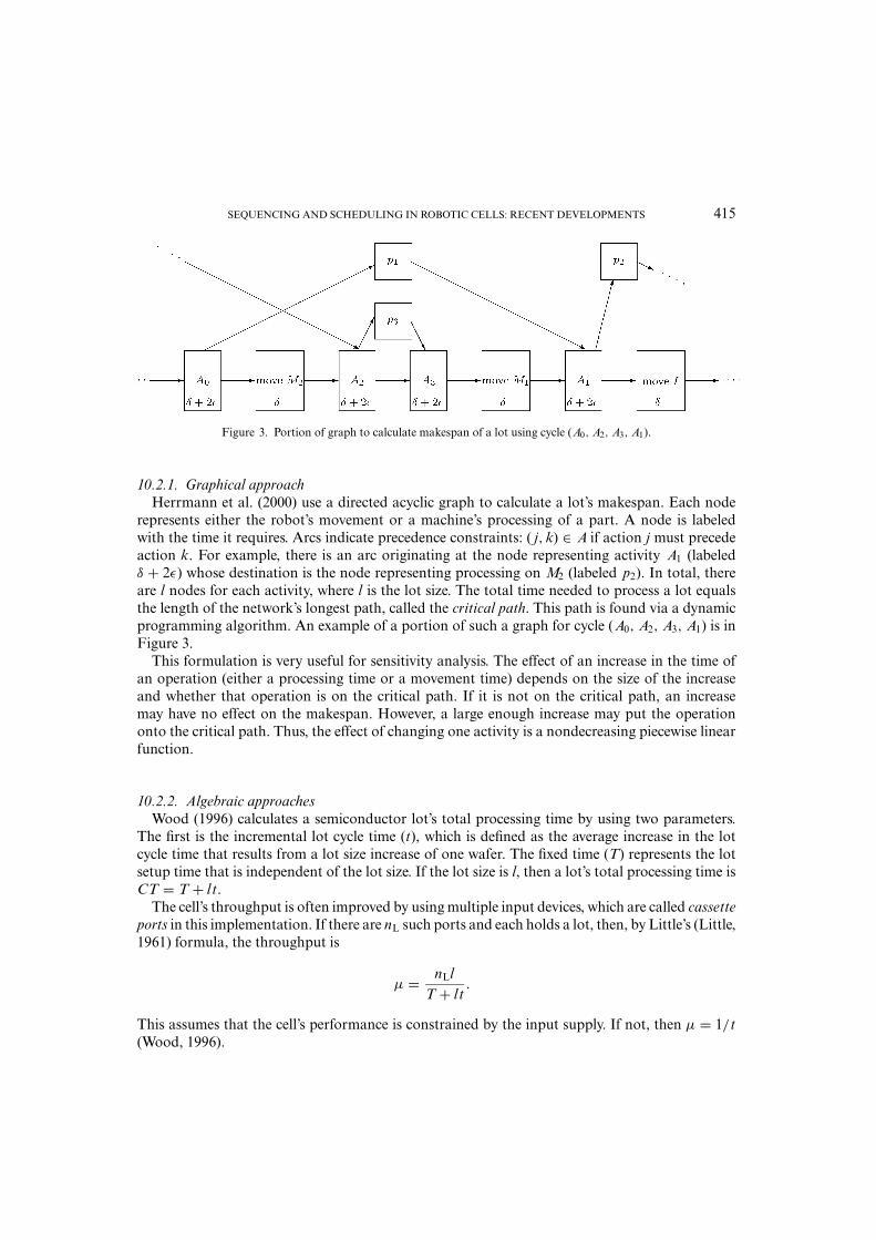
SEQUENCING AND SCHEDULING IN ROBOTIC CELLS: RECENT DEVELOPMENTS 415
Figure 3. Portion of graph to calculate makespan of a lot using cycle (A0, A2, A3, A1).
10.2.1. Graphical approachHerrmann et al. (2000) use a directed acyclic graph to calculate a lot’s makespan. Each node
represents either the robot’s movement or a machine’s processing of a part. A node is labeledwith the time it requires. Arcs indicate precedence constraints: ( j, k) ∈ A if action j must precedeaction k. For example, there is an arc originating at the node representing activity A1 (labeledδ + 2ε) whose destination is the node representing processing on M2 (labeled p2). In total, thereare l nodes for each activity, where l is the lot size. The total time needed to process a lot equalsthe length of the network’s longest path, called the critical path. This path is found via a dynamicprogramming algorithm. An example of a portion of such a graph for cycle (A0, A2, A3, A1) is inFigure 3.
This formulation is very useful for sensitivity analysis. The effect of an increase in the time ofan operation (either a processing time or a movement time) depends on the size of the increaseand whether that operation is on the critical path. If it is not on the critical path, an increasemay have no effect on the makespan. However, a large enough increase may put the operationonto the critical path. Thus, the effect of changing one activity is a nondecreasing piecewise linearfunction.
10.2.2. Algebraic approachesWood (1996) calculates a semiconductor lot’s total processing time by using two parameters.
The first is the incremental lot cycle time (t), which is defined as the average increase in the lotcycle time that results from a lot size increase of one wafer. The fixed time (T) represents the lotsetup time that is independent of the lot size. If the lot size is l, then a lot’s total processing time isCT = T + lt.
The cell’s throughput is often improved by using multiple input devices, which are called cassetteports in this implementation. If there are nL such ports and each holds a lot, then, by Little’s (Little,1961) formula, the throughput is
µ = nLlT + lt
.
This assumes that the cell’s performance is constrained by the input supply. If not, then µ = 1/t(Wood, 1996).
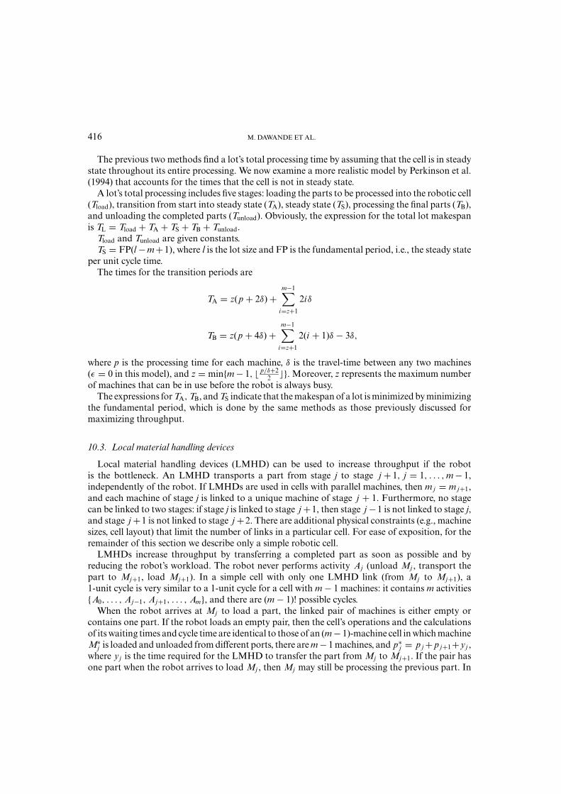
416 M. DAWANDE ET AL.
The previous two methods find a lot’s total processing time by assuming that the cell is in steadystate throughout its entire processing. We now examine a more realistic model by Perkinson et al.(1994) that accounts for the times that the cell is not in steady state.
A lot’s total processing includes five stages: loading the parts to be processed into the robotic cell(Tload), transition from start into steady state (TA), steady state (TS), processing the final parts (TB),and unloading the completed parts (Tunload). Obviously, the expression for the total lot makespanis TL = Tload + TA + TS + TB + Tunload.
Tload and Tunload are given constants.TS = FP(l −m +1), where l is the lot size and FP is the fundamental period, i.e., the steady state
per unit cycle time.The times for the transition periods are
TA = z(p + 2δ) +m−1∑
i=z+1
2iδ
TB = z(p + 4δ) +m−1∑
i=z+1
2(i + 1)δ − 3δ,
where p is the processing time for each machine, δ is the travel-time between any two machines(ε = 0 in this model), and z = min{m − 1, p/δ+2
2 �}. Moreover, z represents the maximum numberof machines that can be in use before the robot is always busy.
The expressions for TA, TB, and TS indicate that the makespan of a lot is minimized by minimizingthe fundamental period, which is done by the same methods as those previously discussed formaximizing throughput.
10.3. Local material handling devices
Local material handling devices (LMHD) can be used to increase throughput if the robotis the bottleneck. An LMHD transports a part from stage j to stage j + 1, j = 1, . . . , m − 1,independently of the robot. If LMHDs are used in cells with parallel machines, then m j = m j+1,and each machine of stage j is linked to a unique machine of stage j + 1. Furthermore, no stagecan be linked to two stages: if stage j is linked to stage j +1, then stage j −1 is not linked to stage j,and stage j +1 is not linked to stage j +2. There are additional physical constraints (e.g., machinesizes, cell layout) that limit the number of links in a particular cell. For ease of exposition, for theremainder of this section we describe only a simple robotic cell.
LMHDs increase throughput by transferring a completed part as soon as possible and byreducing the robot’s workload. The robot never performs activity Aj (unload Mj , transport thepart to Mj+1, load Mj+1). In a simple cell with only one LMHD link (from Mj to Mj+1), a1-unit cycle is very similar to a 1-unit cycle for a cell with m − 1 machines: it contains m activities{A0, . . . , Aj−1, Aj+1, . . . , Am}, and there are (m − 1)! possible cycles.
When the robot arrives at Mj to load a part, the linked pair of machines is either empty orcontains one part. If the robot loads an empty pair, then the cell’s operations and the calculationsof its waiting times and cycle time are identical to those of an (m − 1)-machine cell in which machineM∗
j is loaded and unloaded from different ports, there are m − 1 machines, and p∗j = p j + p j+1+yj ,
where yj is the time required for the LMHD to transfer the part from Mj to Mj+1. If the pair hasone part when the robot arrives to load Mj , then Mj may still be processing the previous part. In
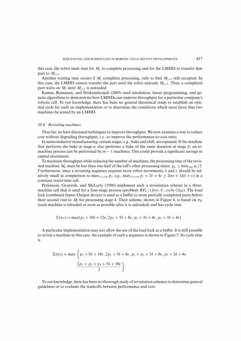
SEQUENCING AND SCHEDULING IN ROBOTIC CELLS: RECENT DEVELOPMENTS 417
this case, the robot must wait for Mj to complete processing and for the LMHD to transfer thatpart to Mj+1.
Another waiting time occurs if Mj completes processing, only to find Mj+1 still occupied. Inthis case, the LMHD cannot transfer the part until the robot unloads Mj+1. Thus, a completedpart waits on Mj until Mj+1 is unloaded.
Kumar, Ramanan, and Sriskandarajah (2005) used simulation, linear programming, and ge-netic algorithms to demonstrate how LMHDs can improve throughput for a particular company’srobotic cell. To our knowledge, there has been no general theoretical study to establish an opti-mal cycle for such an implementation or to determine the conditions which most favor that twomachines be joined by an LMHD.
10.4. Revisiting machines
Thus far, we have discussed techniques to improve throughput. We now examine a way to reducecost without degrading throughput, i.e., to improve the performance-to-cost ratio.
In semiconductor manufacturing, certain stages, e.g., bake and chill, are repeated. If the machinethat performs the bake at stage α also performs a bake of the same duration at stage β, an m-machine process can be performed by m − 1 machines. This could provide a significant savings incapital investment.
To maintain throughput while reducing the number of machines, the processing time of the revis-ited machine Mα must be less than one-half of the cell’s other processing times: pα ≤ mini �=α pi/2.Furthermore, since a revisiting sequence requires more robot movements, δ and ε should be rel-atively small in comparison to max1≤i≤m pi , e.g., max1≤i≤m pi + 3δ + 4ε ≥ 2(m + 1)(δ + ε) in aconstant travel-time cell.
Perkinson, Gyurcsik, and McLarty (1996) implement such a revisitation scheme in a three-machine cell that is used for a four-stage process (problem RF4 | ( free, C, cyclic-1)|µ). The loadlock (combined Input/Output device) is used as a buffer to store partially completed parts beforetheir second visit to M1 for processing stage 4. Their scheme, shown in Figure 4, is based on πD
(each machine is reloaded as soon as possible after it is unloaded) and has cycle time
Tc(π1) = max{p1 + 10δ + 12ε, 2p1 + 5δ + 8ε, p2 + 3δ + 4ε, p3 + 3δ + 4ε}.
A particular implementation may not allow the use of the load lock as a buffer. It is still possibleto revisit a machine in this case. An example of such a sequence is shown in Figure 5. Its cycle timeis
Tc(π2) = max{
p1 + 8δ + 10ε, 2p1 + 5δ + 8ε, p1 + p2 + 5δ + 8ε, p3 + 3δ + 4ε,
2p1 + p2 + p3 + 5δ + 10ε
2
}
.
To our knowledge, there has been no thorough study of revisitation schemes to determine generalguidelines or to evaluate the tradeoffs between performance and cost.
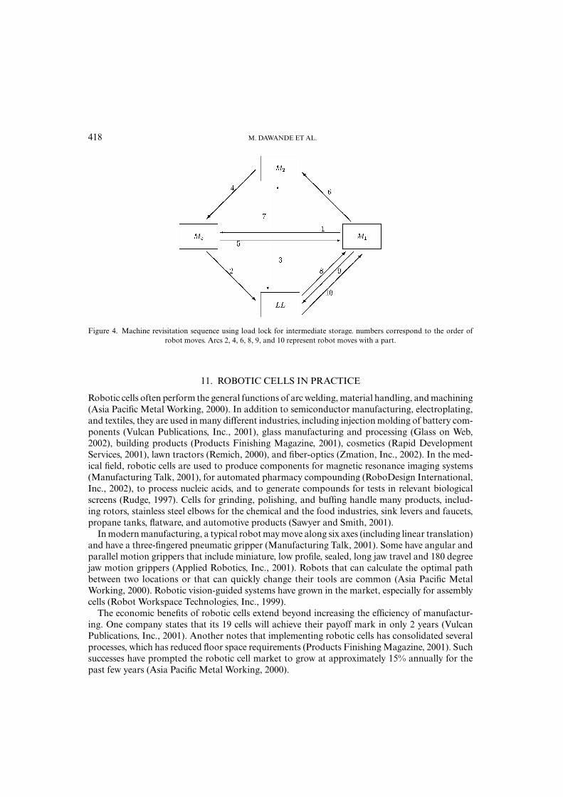
418 M. DAWANDE ET AL.
Figure 4. Machine revisitation sequence using load lock for intermediate storage. numbers correspond to the order ofrobot moves. Arcs 2, 4, 6, 8, 9, and 10 represent robot moves with a part.
11. ROBOTIC CELLS IN PRACTICE
Robotic cells often perform the general functions of arc welding, material handling, and machining(Asia Pacific Metal Working, 2000). In addition to semiconductor manufacturing, electroplating,and textiles, they are used in many different industries, including injection molding of battery com-ponents (Vulcan Publications, Inc., 2001), glass manufacturing and processing (Glass on Web,2002), building products (Products Finishing Magazine, 2001), cosmetics (Rapid DevelopmentServices, 2001), lawn tractors (Remich, 2000), and fiber-optics (Zmation, Inc., 2002). In the med-ical field, robotic cells are used to produce components for magnetic resonance imaging systems(Manufacturing Talk, 2001), for automated pharmacy compounding (RoboDesign International,Inc., 2002), to process nucleic acids, and to generate compounds for tests in relevant biologicalscreens (Rudge, 1997). Cells for grinding, polishing, and buffing handle many products, includ-ing rotors, stainless steel elbows for the chemical and the food industries, sink levers and faucets,propane tanks, flatware, and automotive products (Sawyer and Smith, 2001).
In modern manufacturing, a typical robot may move along six axes (including linear translation)and have a three-fingered pneumatic gripper (Manufacturing Talk, 2001). Some have angular andparallel motion grippers that include miniature, low profile, sealed, long jaw travel and 180 degreejaw motion grippers (Applied Robotics, Inc., 2001). Robots that can calculate the optimal pathbetween two locations or that can quickly change their tools are common (Asia Pacific MetalWorking, 2000). Robotic vision-guided systems have grown in the market, especially for assemblycells (Robot Workspace Technologies, Inc., 1999).
The economic benefits of robotic cells extend beyond increasing the efficiency of manufactur-ing. One company states that its 19 cells will achieve their payoff mark in only 2 years (VulcanPublications, Inc., 2001). Another notes that implementing robotic cells has consolidated severalprocesses, which has reduced floor space requirements (Products Finishing Magazine, 2001). Suchsuccesses have prompted the robotic cell market to grow at approximately 15% annually for thepast few years (Asia Pacific Metal Working, 2000).
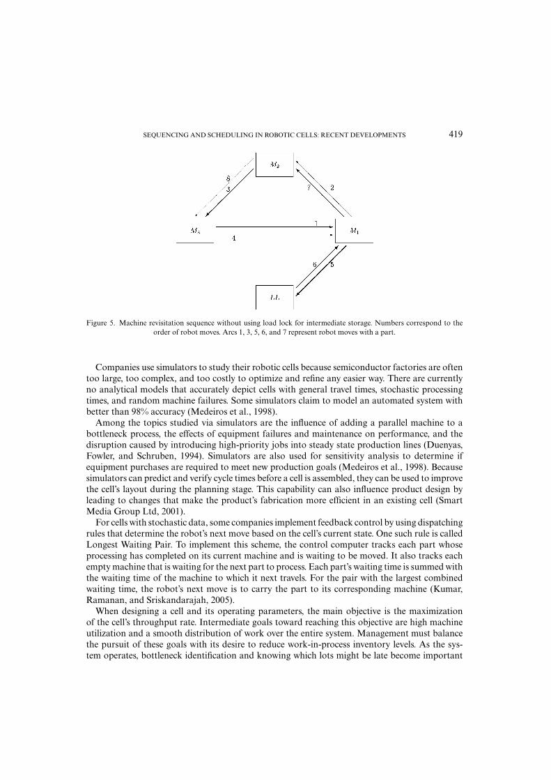
SEQUENCING AND SCHEDULING IN ROBOTIC CELLS: RECENT DEVELOPMENTS 419
Figure 5. Machine revisitation sequence without using load lock for intermediate storage. Numbers correspond to theorder of robot moves. Arcs 1, 3, 5, 6, and 7 represent robot moves with a part.
Companies use simulators to study their robotic cells because semiconductor factories are oftentoo large, too complex, and too costly to optimize and refine any easier way. There are currentlyno analytical models that accurately depict cells with general travel times, stochastic processingtimes, and random machine failures. Some simulators claim to model an automated system withbetter than 98% accuracy (Medeiros et al., 1998).
Among the topics studied via simulators are the influence of adding a parallel machine to abottleneck process, the effects of equipment failures and maintenance on performance, and thedisruption caused by introducing high-priority jobs into steady state production lines (Duenyas,Fowler, and Schruben, 1994). Simulators are also used for sensitivity analysis to determine ifequipment purchases are required to meet new production goals (Medeiros et al., 1998). Becausesimulators can predict and verify cycle times before a cell is assembled, they can be used to improvethe cell’s layout during the planning stage. This capability can also influence product design byleading to changes that make the product’s fabrication more efficient in an existing cell (SmartMedia Group Ltd, 2001).
For cells with stochastic data, some companies implement feedback control by using dispatchingrules that determine the robot’s next move based on the cell’s current state. One such rule is calledLongest Waiting Pair. To implement this scheme, the control computer tracks each part whoseprocessing has completed on its current machine and is waiting to be moved. It also tracks eachempty machine that is waiting for the next part to process. Each part’s waiting time is summed withthe waiting time of the machine to which it next travels. For the pair with the largest combinedwaiting time, the robot’s next move is to carry the part to its corresponding machine (Kumar,Ramanan, and Sriskandarajah, 2005).
When designing a cell and its operating parameters, the main objective is the maximizationof the cell’s throughput rate. Intermediate goals toward reaching this objective are high machineutilization and a smooth distribution of work over the entire system. Management must balancethe pursuit of these goals with its desire to reduce work-in-process inventory levels. As the sys-tem operates, bottleneck identification and knowing which lots might be late become important
420 M. DAWANDE ET AL.
objectives (Duenyas, Fowler, and Schruben, 1994). General guidelines for applying operations re-search techniques to planning, designing, and operating robotic cells can be found in Hall et al.(1999).
12. OPEN PROBLEMS: RECOMMENDATIONS FOR FUTURE STUDY
We now summarize some open problems in the field of robotic cell sequencing and scheduling.
� Simple robotic cells: As mentioned in Section 3, at least nine different types of simplerobotic cells with single gripper robots have been studied in the literature, depending onthe pickup criterion (no-wait, interval, or free-pickup) and the travel-time metric (additive,constant, or Euclidean). For additive and constant travel-time cells with free-pickup, thereexist polynomial-time algorithms for finding an optimal 1-unit cycle (Crama and van de Klun-dert, 1997a; Dawande, Sriskandarajah and Sethi, 2002) (problems RFm|(free, A, cyclic-1)|µand RFm|( free, C, cyclic-1|µ). For such cells, two fundamental problems remain open: (1) Fora given k, k ≥ 2, finding an algorithm that produces an optimal k-unit cycle and (2) Findingan algorithm that produces an optimal cycle among the class of all cyclic solutions (prob-lems RFm|( free, A, cyclic-k)|µ and RFm|( free, C, cyclic-k)|µ). The complexity status of theseproblems is unknown. It is conceivable that mathematical programming formulations may beof help in solving these problems. To the best of our knowledge, there is no known linear orinteger programming formulation for the optimal k-unit cycle problem, k ≥ 1, for any cellswith free-pickup.For interval robotic cells with additive travel-times (problem RFm|(interval, A, cyclic-1)|µ),the robot move sequencing problem is NP-hard (Crama and van de Klundert, 1997b). Thisimplies that the problem is NP-hard for interval cells with Euclidean travel-times, too (prob-lem RFm|(interval, E, cyclic-1)|µ). Consequently, approximation algorithms that guarantee anear-optimal solution in polynomial time are of interest for such cells. No results have beenpublished for interval cells with constant travel-time.
For Euclidean no-wait cells, polynomial algorithms to find an optimal 1-unit cycle (Levner,Kats, and Levit, 1997) (problem RFm|(no-wait, E, cyclic-1)|µ) and an optimal 2-unit cycle(Che, Chu, and Levner, 2003) (problem RFm|(no-wait, E, cyclic-2)|µ) have been developed.Finding an optimal k-unit cycle over all k, k ≥ 1, (problem RFm|(no-wait, E, cyclic-k)|µ) isan open problem, although Agnetis (Agnetis, 2000) has conjectured that k < m for such anoptimal cycle. Mangione, Brauner, and Penz (2003) prove this conjecture for certain balanced(pi = p, ∀i ) and regular additive no-wait cells.
� Simple robotic cells with multiple part-types: We saw in Section 6 that for multiple part-typecells, two subproblems arise: part scheduling and robot move sequencing. Given a robotmove sequence, finding the optimal part schedule is NP-hard for m ≥ 3 (Hall, Kamoun,and Sriskandarajah, 1997). The complementary problem of finding an optimal robot movesequence given a part schedule has not been studied for m ≥ 3.
For cells that process multiple part-types with m ≥ 3, all results in Section 6.3 con-cern CRM sequences (problem RFm|(free, A, MP, CRM)|µ). There has been no researchon finding the optimal part schedule for a non-CRM MPS robot move sequence (problemRFm|(free, A, MP, cyclic-k)|µ). Such a result would provide insight into how close the bestCRM sequence is to the optimal MPS cyclic solution. This problem, however, is a generaliza-tion of the optimal k-unit cycle problem, which is also open.
SEQUENCING AND SCHEDULING IN ROBOTIC CELLS: RECENT DEVELOPMENTS 421
� Robotic cells with parallel machines: The optimal cyclic solution has been foundonly for a special case (pi ≥ δ, ∀i ) in free-pickup constant travel-time cells (seeSection 8 or Geismar, Dawande, and Sriskandarajah (2004a)). No studies have beenpublished that address more general free-pickup constant travel-time cells (problemRFm(m1, m2, . . . , mm)|(free, C, cyclic-k)|µ) or any free-pickup cells with additive travel-times(problem RFm(m1, m2, . . . , mm)|( free, A, cyclic-k)|µ).For cases in which finding the optimal move sequence in a simple robotic cell isknown to be NP-hard (Euclidean free-pickup: RFm(m1, m2, . . . , mm)|(free, E, cyclic-k)|µ,Euclidean interval: RFm(m1, m2, . . . , mm)|(interval, E, cyclic-k)|µ, and additive interval:RFm(m1, m2, . . . , mm)|(interval, E, cyclic-k)|µ), the problems for cells with parallel machinesare NP-hard, too. Finding efficient approximation algorithms remains an open question forthese cases.
There exists a polynomial algorithm to optimize throughput for 1-unit cycles in no-waitsimple robotic cells (Levner, Kats, and Levit, 1997). We know of no work that addresses no-waitrobotic cells with parallel machines (problem RFm(m1, m2, . . . , mm)|(no-wait,∗ , cyclic-k)|µ).
Finding the optimal schedule for processing multiple part-types in roboticcells with parallel machines (for any travel-time or pickup scheme (problemRFm(m1, m2, . . . , mm)|(∗,∗ , MP, cyclic-k)|µ)) is also a generalization of the optimal k-unit cycle problem. Hence, it is currently an open question.
� Stochastic data: In general, one cannot expect deterministic solutions to be optimal forstochastic problems. It is important to find conditions under which deterministic solutionsprovide near-optimal solutions. Finding the best dispatching rule is also an open problem.Another issue concerns random failures of processing machines. Some manufacturers use par-allel machines to provide redundancy. Given each machine’s rate of failure, the distributionof each machine’s repair time, each machine’s cost, and the distribution of each machine’sprocessing time, what is the economically optimal number of machines to have at each stage?Such a calculation should also formulate the economic impact of improved throughput, i.e.,cycle time comparison is a subproblem to the problem of finding the optimal number ofredundant machines. Suri (1985) provides some guidelines for addressing such questions.
� Dual gripper robots: These have not been studied for Euclidean travel-time(problem RF2
m|(∗, E, cyclic-k)|µ) or for interval or no-wait pickup (problemsRF2
m|(interval,∗ , cyclic-k)|µ and RF2m|(no-wait,∗ , cyclic-k)|µ). It would also be interest-
ing to examine the use of dual gripper robots in cells with multiple robots and parallelmachines. Such a study could be based on the results in Geismar, Sriskandarajah, andRamanan (2004d).
� Flexible robotic cells: Recent work has studied robotic cells that are open shops, rather thanflowshops. In these cells the operations can be performed in any order, and each machine canbe configured to perform any of the operations. Geismar et al. (2004c) show that for m = 3and m = 4, the largest productivity gain that can be realized by changing the assignmentof operations to machines is 14 2
7 %. It is unknown whether this upper bound holds form ≥ 5.
� Implementation issues: The implementation issues discussed in Section 10 have open problems,including the following:
- The optimal use of local material handling devices remains an open question.- The economic and performance trade-offs concerning schedules that revisit machines bear
further study.

422 M. DAWANDE ET AL.
13. CONCLUDING REMARKS
We have presented a survey of recent work in robotic cell scheduling problems. We have discussedbasic properties of robotic cells and detailed the tools most often used to analyze them. In so doingwe have provided guidelines for determining the optimal policies for a variety of implementations.Furthermore, we have furnished a framework that future studies may employ to analyze new cellswith different characteristics. This should also serve as a useful introduction to researchers andpractitioners of the field. The material presented in this survey is the subject of a forthcoming bookby Dawande et al. (to appear).
The field of robotic cell scheduling has grown rapidly over the past decade. As manufacturershave employed them in greater numbers and greater varieties, analysts have developed new modelsand new techniques to maximize these cells’ economic utility. Competitive pressures will result inthe development of more advanced cells and, hence, more sophisticated studies. Therefore, roboticcell scheduling should continue to attract the attention of a growing number of researchers.
ACKNOWLEDGMENT
The authors wish to thank the two anonymous referees and the associate editor, whose commentshave significantly improved the content and the presentation of this paper.
APPENDIX: PROOF OF THEOREM 5
Ta(πD) = max{4mδ + 2(m + 1)ε, max pi + 4(δ + ε)}. If Ta(πD) = max pi + 4(δ + ε), then it is opti-mal by Theorem 3. Assume Ta(πD) = 4mδ + 2(m + 1)ε. The set of pyramidal cycles contains anoptimal cycle (Crama and van de Klundert, 1997a). Note that activity Am is always considered tobe an uphill activity, so πD is the pyramidal cycle that corresponds to U = {m}.
Consider a general pyramidal cycle πp �= πD, and let i, 1 ≤ i ≤ m − 1, be the smallest index ofan uphill activity for cycle πp. This implies that the form of cycle πp is either
A0 Ai Ai+1 . . . Am . . . Ai−1 Ai−2 . . . A1 or
A0 Ai . . . Am . . . Ai+1 Ai−1 Ai−2 . . . A1.
In either case, we can easily calculate lower bounds on the durations of the following nonoverlap-ping segments of the cycle:
1. from the start of activity Ai until the start of activity Ai+1 : δ + 2ε + pi+1
2. from the start of activity Ai+1 until the start of activity Ai−1 : 4δ + 2ε
3. from the start of activity Ai−1 until the start of activity Ai : δ + 2ε + pi
Thus, we have the following lower bound for the cycle time:
T(πp) ≥ pi + pi+1 + 6δ + 6ε ≥ 4mδ + 2(m + 1)ε = T(πD)
REFERENCES
Agnetis, A., “Scheduling no-wait robotic cells with two and three machines,” European Journal of Operational Research,123, 303–314 (2000).
Agnetis, A. and D. Pacciarelli, “Part sequencing in three-machine no-wait robotic cells,” Operations Research Letters, 27,185–192 (2000).
SEQUENCING AND SCHEDULING IN ROBOTIC CELLS: RECENT DEVELOPMENTS 423
Akcalı, E., K. Nemoto, and R. Uzsoy, “Cycle-time improvements for photolithography process in semiconductor manu-facturing,” IEEE Transactions on Semiconductor Manufacturing, 14, 48–56 (2001).
Aneja, Y. P. and H. Kamoun, “Scheduling of parts and robot activities in a two-machine robotic cell,” Computers andOperations Research, 26, 297–312 (1999).
Asfahl, C. R., Robots and Manufacturing Automation, John Wiley & Sons, New York, NY, 1985.Baumann, W., R. Birner, J. Haensler, R. P. Hartmann, and A. B. Stevens, “Operating and idle times for cyclic multi-machine
servicing,” The Industrial Robot, 44–49 (1981).Bedini, R., G. G. Lisini, and P. Sterpos, “Optimal programming of working cycles for industrial robots,” Journal of
Mechanical Design. Transactions of the ASME, 101, 250–257 (1979).B�lazewicz, J., H. Eiselt, G. Finke, G. LaPorte, and J. Weglarz. “Scheduling tasks and vehicles in a flexible manufacturing
system,” International Journal of Flexible Manufacturing Systems, 4, 5–16 (1991).B�lazewicz, J., S. P. Sethi, and C. Sriskandarajah, “Scheduling of robot moves and parts in a robotic cell,” in K. E. Stecke
and R. Suri (eds.), Proceedings of the Third ORSA/TIMS Conference on Flexible Manufacturing Systems: OperationsResearch Models and Applications (Ann Arbor, MI), Elsevier Science Publishers, B.V., Amsterdam, The Netherlands,1989, pp. 281–286.
Brauner, N. and G. Finke, “Final results on the one-cycle conjecture in robotic cells,” Internal note, Laboratoire LEIBNIZ,Institut IMAG, Grenoble, France, 1997.
Brauner, N. and G. Finke, “Cyclic scheduling in a robotic flowshop,” in Proceedings IEPM’97, International Conferenceon Industrial Engineering and Production Management, Lyon, France, 1997, vol.1, pp. 439–449.
Brauner, N. and G. Finke, “On a conjecture in robotic cells: new simplified proof for the three-machine case,” INFOR,37(1), 20–36 (1999).
Brauner, N. and G. Finke, “Optimal moves of the material handling system in a robotic cell,” International Journal ofProduction Economics, 74, 269–277 (2001a).
Brauner, N. and G. Finke, “Cycles and permutations in robotic cells,” Mathematical and Computer Modeling, 34, 565–591(2001b).
Brauner, N., G. Finke, and W. Kubiak, “Complexity of one-cycle robotic flow-shops,” Journal of Scheduling, 6, 355–371(2003).
Che, A., C. Chu, and F. Chu, “Multicyclic hoist scheduling with constant processing times,” IEEE Transactions on Roboticsand Automation, 18(1), 69–80 (2002).
Che, A., C. Chu, and E. Levner, “A polynomial algorithm for 2-degree cyclic robot scheduling,” European Journal ofOperational Research, 145(1), 31–44 (2003).
Chen, H., C. Chu, and J. Proth, “Cyclic scheduling with time window constraints,” IEEE Transactions on Robotics andAutomation, 14(1), 144–152 (1998).
Claybourne, B. H., “Scheduling robots in flexible manufacturing cells,” CME Automation, 30(5), 36–40 (1983).Crama, Y., “Combinatorial optimization models for production scheduling in automated manufacturing systems,” Euro-
pean Journal of Operational Research, 99, 136–153 (1997).Crama, Y., V. Kats, J. van de Klundert, and E. Levner, “Cyclic scheduling in robotic flowshops,” Annals of Operations
Research: Mathematics of Industrial Systems, 96, 97–124 (2000).Crama, Y. and J. van de Klundert, “Cyclic scheduling of identical parts in a robotic cell,” Operations Research, 6, 952–965
(1997a).Crama, Y. and J. van de Klundert, “Robotic flowshop scheduling is strongly NP-complete,” in W. K. Klein Haneveld et al.
(eds.), Ten Years LNMB, CWI Tract, Amsterdam, 1997b, pp. 277–286.Crama, Y. and J. van de Klundert, “Cyclic scheduling in 3-machine robotic flowshops,” Journal of Scheduling, 2, 35–54
(1999).Dawande, M., N. Geismar, and S. Sethi, “Dominance of cyclic solutions and some open problems in scheduling bufferless
robotic cells,” to appear in SIAM Review, 2006a.Dawande, M., N. Geismar, S. Sethi, and C. Sriskandarajah, Throughput Optimization in Robotic Cells, Springer, to
appear.Dawande, M., C. Sriskandarajah, and S. Sethi, “On throughput maximization in constant travel-time robotic cells,”
Manufacturing and Service Operations Management, 4(4), 296–312 (2002).Devedzic, V., “A knowledge-based system for the strategic control level of robots in flexible manufacturing cell,” Interna-
tional Journal of Flexible Manufacturing Systems, 2(4), 263–287 (1990).Dixon, C. and S. D. Hill, “Work-cell cycle-time analysis in a flexible manufacturing system,” in Proceedings of the Pacific
Conference in Manufacturing, Sydney and Melbourne, Australia, 1990, vol. 1, pp.182–189.
424 M. DAWANDE ET AL.
Drobouchevitch, I. G., S. Sethi, and C. Sriskandarajah, “Scheduling dual gripper robotic cell: 1-unit cycles,” to appear inEuropean Journal of Operational Research, 2005.
Drobouchevitch, I. G., S. Sethi, J. Sidney, and C. Sriskandarajah, “A note on scheduling multiple parts in two-machinedual gripper robotic cell: Heuristic algorithm and performance guarantee,” International Journal of Operations andQuantitative Management, 10(4), 297–314 (2004).
Duenyas, I., J. W. Fowler, and L. W. Schruben, “Planning and scheduling in Japanese semiconductor manufacturing,”Journal of Manufacturing Systems, 1994, pp. 323–333.
Finke, G., C. Gueguen, and N. Brauner, “Robotic cells with buffer space,” in R. O’Connor and P. Magee (eds.), ECCO IXConference Proceedings, Dublin City University, 1996.
Garey, M. R. and D. S. Johnson, Computers and Intractability: A Guide to the Theory of NP-Completeness, W. H. Freemanand Company, San Francisco, 1979.
Geismar, H. N., M. Dawande, and C. Sriskandarajah, “Robotic cells with parallel machines: Throughput maximization inconstant travel-time cells,” Journal of Scheduling, 7, 375–395 (2004a).
Geismar, H. N., M. Dawande, and C. Sriskandarajah, “Approximation algorithms for k-unit cyclic solutions in roboticcells,” European Journal of Operational Research, 162, 291–309 (2005).
Geismar, H. N., M. Dawande, and C. Sriskandarajah, “Scheduling constant travel-time dual gripper robotic cells withparallel machines,” Working Paper, School of Management, University of Texas at Dallas, 2004b.
Geismar, H. N., S. P. Sethi, J. B. Sidney, and C. Sriskandarajah, “A note on productivity gains in flexible robotic cells,”Working Paper, School of Management, University of Texas at Dallas, 2004c.
Geismar, H. N., C. Sriskandarajah, and N. Ramanan, “Increasing throughput for robotic cells with parallel machines andmultiple robots,” IEEE Transactions on Automation Science and Engineering, 1(1), 84–89 (2004d).
Gilmore, P. and R. Gomory, “Sequencing a one-state variable machine: A solvable case of the traveling salesman problem,”Operations Research, 12, 675–679 (1964).
Graham, R. L., E. L. Lawler, J. K. Lenstra, and A. H. G. Rinnoy Kan, “Optimization and approximation in deterministicsequencing and scheduling: A survey,” Annals of Discrete Mathematics, 5, 287–326 (1979).
Hall, N., “Operations research techniques for robotic systems,” in S. Y. Nof (ed.), Handbook of Industrial Robotics, 2nded., John Wiley and Sons, 1999.
Hall, N. G., H. Kamoun, and C. Sriskandarajah, “Scheduling in robotic cells: Classification, two- and three-machine cells,”Operations Research, 45, 421–439 (1997).
Hall, N. G., H. Kamoun, and C. Sriskandarajah, “Scheduling in robotic cells: Complexity and steady state analysis,”European Journal of Operational Research, 109, 43–63 (1998).
Hall, N. G. and C. Sriskandarajah, “A survey of machine scheduling problems with blocking and no-wait in process,”Operations Research, 44(3), 510–525 (1996).
Hall, N. G., C. Potts, and C. Sriskandarajah, “Parallel machine scheduling with a common server,” Discrete AppliedMathematics, 102, 223–243 (2000).
Herrmann, J., N. Chandrasekaran, B. Conaghan, M. Nguyen, G. Rubloff, and R. Shi, “Evaluating the impact of processchanges on cluster tool performance,” IEEE Transactions on Semiconductor Manufacturing, 13, 181–192 (2000).
Ioachim, I. and F. Soumis, “Schedule efficiency in a robotic production cell,” The International Journal of Flexible Manu-facturing Systems, 7, 5–26 (1995).
Kamoun, H., “Scheduling in repetitive manufacturing systems: Complexity, heuristic algorithms and system design,” Ph.D.Thesis, Graduate Department of Industrial Engineering, University of Toronto, 1994.
Kamoun, H., N. G. Hall, and C. Sriskandarajah, “Scheduling in robotic cells: Heuristics and cell design,” OperationsResearch, 47, 821–835 (1999).
Kats, V., “An exact optimal cyclic scheduling algorithm for multioperator service of a production line, part 2,” Automationand Remote Control, 42(4), 538–543 (1982).
Kats, V. and E. Levner, “Minimizing the number of robots to meet a given schedule,” Annals of Operations Research, 69,209–226 (1997).
Kats, V. and E. Levner, “Polynomial algorithms for cyclic scheduling of tasks on parallel processors,” in Proceedings of the16th IASTED International Conference on Applied Informatics, Garmisch, Germany, 1998, pp. 302–304.
Kats, V. and E. Levner, “Cycle scheduling in a robotic production line,” Journal of Scheduling, 5, 23–41 (2002).Kats, V., E. Levner, and L. Meyzin, “Multiple-part cyclic hoist scheduling using a sieve method,” IEEE Transactions on
Robotics and Automation, 15(4), 704–713 (1999).Kondoleon, A. S., “Cycle time analysis of robot assembly systems,” in Proceedings of the Ninth Symposium on Industrial
Robots, 1979, pp. 575–587.
SEQUENCING AND SCHEDULING IN ROBOTIC CELLS: RECENT DEVELOPMENTS 425
Kumar, S., N. Ramanan, and C. Sriskandarajah, “Minimizing cycle time in large robotic cells,” IIE Transactions, 37(2),123–136 (2005).
Lawler, E. L., J. K. Lenstra, A. H. G. Rinnooy Kan, and D. B. Shmoys (eds.), The Traveling Salesman Problem: A GuidedTour of Combinatorial Optimization, John Wiley & Sons, Chichester, 1985.
Lei, L. and T. J. Wang, “Determining optimal cyclic hoist schedules in a single-hoist electroplating line,” IIE Transactions,26(2), 25–33 (1994).
Levner, E., V. Kats, and V. Levit, “An improved algorithm for cyclic flowshop scheduling in a robotic cell,” EuropeanJournal of Operational Research, 97, 500–508 (1997).
Little, J. D. C., “A proof for the queuing formula: L = λW,” Operations Research, 9(3), 383–387 (1961).Logendran, R. and C. Sriskandarajah, “Sequencing of robot activities and parts in two-machine robotic cells,” International
Journal of Production Research, 34(12), 3447–3463 (1996).Maimon, O. Z. and S. Y. Nof, “Coordination of robots sharing assembly tasks,” Journal of Dynamic Systems Measurement
and Control. Transactions of the ASME, 107(4), 299–307 (1985).Mangione, F., N. Brauner, and B. Penz, “Optimal cycles for the robotic balanced no-wait flowshop,” in Proceedings
IEPM’03, International Conference of Industrial Engineering and Production Management, Porto, Portugal, May 2003.Medeiros, D. J., E. F. Watson, J. S. Carson, and M. S. Manivannan (eds.), “Operational modeling & simulation in semi-
conductor manufacturing,” in Proceedings of the 1998 Winter Simulation Conference.Miller, R. K., Robots in Industry: Applications for the Electronics Industry, SEAI Institute, New York, 1984.Nof, S. Y. and D. Hannah, “Operational characteristics of multi-robot systems with cooperation,” International Journal of
Production Research, 27(3), 477–492 (1989).Perkinson, T., P. McLarty, R. Gyurcsik, and R. Cavin, “Single-wafer cluster tool performance: An analysis of throughput,”
IEEE Transactions on Semiconductor Manufacturing, 7, 369–373 (1994).Perkinson, T., R. Gyurcsik, and P. McLarty, “Single-wafer cluster tool performance: An analysis of the effects of redundant
chambers and revisitation sequences on throughput,” IEEE Transactions on Semiconductor Manufacturing, 9, 384–400(1996).
Pinedo, M., Scheduling: Theory, Algorithms, and Systems, Prentice Hall, Englewood Cliffs, New Jersey, 1995.Ramanan, N., personal communication, 2002.Rudge, D. A., “The automation of solution phase synthetic chemistry using XP zymate laboratory robotic systems,”
Laboratory Automation and Information Management, 33, 81–86 (1997).Sethi, S. P., C. Sriskandarajah, G. Sorger, J. B�lazewicz, and W. Kubiak, “Sequencing of parts and robot moves in a robotic
cell,” Int. J. Flexible Manufacturing Systems, 4, 331–358 (1992).Sethi, S. P., J. Sidney, and C. Sriskandarajah, “Scheduling in dual gripper robotic cells for productivity gains,” IEEE
Transactions on Robotics and Automation, 17, 324–341 (2001).Sriskandarajah, C., I. G. Drobouchevitch, S. Sethi, and R. Chandrasekaran, “Scheduling multiple parts in a robotic cell
served by a dual gripper robot,” Operations Research, 52, 65–82 (2004).Sriskandarajah, C., N. G. Hall, and H. Kamoun, “Scheduling large robotic cells without buffers,” Annals of Operations
Research, 76, 287–321 (1998).Su, Q. and F. Chen, “Optimal sequencing of double-gripper gantry robot moves in tightly-coupled serial production
systems,” IEEE Transactions on Robotics and Automation, 12, 22–30 (1996).Suri, R., “Quantitative techniques for robotic systems analysis,” in S. Y. Nof (ed.), Handbook of Industrial Robotics, John
Wiley and Sons, 1985, , Vol. I.Van de Klundert, J., Scheduling Problems in Automated Manufacturing, Faculty of Economics and Business Administration,
University of Limburg, Maastricht, The Netherlands, Dissertation no. 96-35, 1996.Venkatesh, S., R. Davenport, P. Foxhoven, and J. Nulman, “A steady-state throughput analysis of cluster tools: Dual-blade
versus single-blade robots,” IEEE Transactions on Semiconductor Manufacturing, 10, 418–424 (1997).Wilhelm, W. E., “Complexity of sequencing tasks in assembly cells attended by one or two robots,” Naval Research Logistics,
34, 721–738 (1987).Wittrock, R. J., “Scheduling algorithms for flexible flow lines,” IBM Journal of Research and Development, 29, 401–412
(1985).Wood, S., “Simple performance models for integrated processing tools,” IEEE Transactions on Semiconductor Manufac-
turing, 9, 320–328 (1996).
426 M. DAWANDE ET AL.
WEB SITES REFERENCES
Applied Robotics, Inc., http://www.arobotics.com/product.html, 2001.Asia Pacific Metal Working, http://www.equipment-news.com/magazines/2000/sep2000/art05.htm, 2000.Glass on Web, http://www.glassonweb.com/articles/article/13/, 2002.Manufacturing Talk, http://www.manufacturingtalk.com/news/bab/bab101.txt, 2001.Manufacturing Talk, http://www.manufacturingtalk.com/news/guy/guy123.txt, 2001.Products Finishing Magazine, http://www.pfonline.com/articles/080103.html, 2001.Rapid Development Services, Inc., http://roboticintegrator.com/, 2001.N. Remich, “The Robotic Ballet,” Appliance Manufacturer, http://www.ammagazine.com, 2000.RoboDesign International, Inc., http://www.robodesign.com/roboarrayer options.htm, 2002.Robot Workspace Technologies, Inc., http://www.rwt.com/RWT Content Files/articles/RWT ASept99ME.html, 1999.Sawyer and Smith Corporation, http://www.buffingandpolishing.com/automaticproducts.htm, 2001.Smart Media Group Ltd, http://www.robotics-technology.com/articlearchive/2001/112001.shtml, 2001.Vulcan Publications, Inc., http://www.ndx.com/article.asp?article id=270 & channel id=6, 2001.Zmation, Inc., http://www.zmation.com/products.htm, 2002.


![A Deep-Sequencing Workflow for the Fast and Efficient … · P72 Genotype WGS Publication Method Coverage 1 NC_001659.2 BA71V Spain 1995 1967 Vero cells I [32] Sanger sequencing N/A](https://img.pdfslide.net/doc/110x75/60d200b53ac94e78843b4602/a-deep-sequencing-workflow-for-the-fast-and-efficient-p72-genotype-wgs-publication.jpg)