Embed Size (px)
Citation preview

Series solutions of ordinary
differential equations
1

Second-order linear ordinary differentialequations
Any homogeneous second-order linear ODE can be
written in the form
y′′ + p(x)y′ + q(x)y = 0, (1)
where y′ = dy/dx and p(x) and q(x) are given
functions of x. The most general solution to Eq. (1)
is
y(x) = c1y1(x) + c2y2(x), (2)
where y1(x) and y2(x) are linearly independent
solutions of Eq. (1), and c1 and c2 are constants.
Their linear independence may be verified by the
evaluation of the Wronskian
W (x) =
∣∣∣∣∣∣y1 y2
y′1 y′2
∣∣∣∣∣∣= y1y
′2 − y2y
′1. (3)
If W (x) 6= 0 in a given interval, then y1 and y2 are
linearly independent in that interval.
2

By differentiating Eq. (3) with respect to x, we
obtain
W ′ = y1y′′2 + y′1y
′2 − y2y
′′1 − y′2y
′1 = y1y
′′2 − y′′1 y2.
Since both y1 and y2 satisfy Eq. (1), we may
substitute for y′′1 and y′′2 , which yields
W ′ = −y1(py′2 + qy2) + (py′1 + qy1)y2
= −p(y1y′2 − y′1y2) = −pW.
Integrating, we find
W (x) = C exp{−
∫ x
p(u) du
}, (4)
where C is a constant. If p(x) ≡ 0, we obtain W =constant.
3

Ordinary and singular points of an ODE
Consider the second-order linear homogeneous ODE
y′′ + p(z)y′ + q(z) = 0, (5)
where the functions are complex functions of a
complex variable z. If at some point z = z0 the
functions p(z) and q(z) are finite, and can be
expressed as complex power series
p(z) =∞∑
n=0
pn(z − z0)n, q(z) =∞∑
n=0
qn(z − z0)n,
then p(z) and q(z) are said to be analytic at z = z0,
and this point is called an ordinary point of the
ODE. If, however, p(z) or q(z), or both, diverge at
z = z0, then it is called a singular point of the ODE.
4

Even if an ODE is singular at a given point z = z0,
it may still possess a non-singular (finite) solution at
that point. The necessary and sufficient condition
for such a solution to exist is that (z − z0)p(z) and
(z − z0)2q(z) are both analytic at z = z0. Singular
points that have this property are regular singular
points, whereas any singular point not satisfying
both these criteria is termed an irregular or essential
singularity.
5

Example
Legendre’s equation has the form
(1− z2)y′′ − 2zy′ + l(l + 1)y = 0. (6)
where l is a constant. Show that z = 0 is an
ordinary point and z = ±1 are regular singular
points of this equation.
Answer
We first divide through by 1− z2 to put the
equation into our standard form, Eq. (5):
y′′ − 2z
1− z2y′ +
l(l + 1)1− z2
y = 0.
Comparing with Eq. (5), we identify
p(z) =−2z
1− z2=
−2z
(1 + z)(1− z)
q(z) =l(l + 1)1− z2
=l(l + 1)
(1 + z)(1− z).
6

By inspection, p(z) and q(z) are analytic at z = 0,
which is therefore an ordinary point, but both
diverge for z = ±1, which are thus singular points.
However, at z = 1, we see that both (z − 1)p(z)and (z − 1)2q(z) are analytic, and hence z = 1 is a
regular singular point. Similarly, z = −1 is a regular
singular point.
7

Example
Show that the Legendre’s equation has a regular
singularity at |z| → ∞.
Answer
Letting w = 1/z, the derivatives with respect to z
become
dy
dz=
dy
dw
dw
dz= − 1
z2
dy
dw= −w2 dy
dw,
d2y
dz2=
dw
dz
d
dw
(dy
dz
)
= −w2
(−2w
dy
dw− w2 d2y
dw2
)
= w3
(2
dy
dw+ w
d2y
dw2
).
If we substitute these derivatives into Legendre’s
equation Eq. (6) we obtain(
1− 1w2
)w3
(2
dy
dw+ w
d2y
dw2
)
+21w
w2 dy
dw+ l(l + 1)y = 0,
8

which simplifies to give
w2(w2 − 1)dy
dw2+ 2w3 dy
dw+ l(l + 1)y = 0.
Dividing through by w2(w2 − 1), and comparing
with Eq. (5), we identify
p(w) =2w
w2 − 1,
q(w) =l(l + 1)
w2(w2 − 1).
At w = 0, p(w) is analytic but q(w) diverges, and
so the point |z| → ∞ is a singular point of
Legendre’s equation. However, since wp and w2q
are both analytic at w = 0, |z| → ∞ is a regular
singular point.
9

Equation Regular Essential
singularities singularities
Legendre
(1− z2)y′′
−2zy′ + l(l + 1)y = 0 −1, 1,∞Chebyshev
(1− z2)y′′
−zy′ + n2y = 0 −1, 1,∞Bessel
z2y′′ + zy′
+(z2 − ν2)y = 0 0 ∞Laguerre
zy′′ + (1− z)y′
+αy = 0 0 ∞Simple harmonic
oscillator
y′′ + ω2y = 0 ∞
10

Series solutions about an ordinary point
If z = z0 is an ordinary point of Eq. (5), then every
solution y(z) of the equation is also analytic at
z = z0. We shall take z0 as the origin. If this is not
the case, then a substitution Z = z− z0 will make it
so. Then y(z) can be written as
y(z) =∞∑
n=0
anzn. (7)
Such a power series converges for |z| < R, where R
is the radius of convergence.
Since every solution of Eq. (5) is analytic at an
ordinary point, it is always possible to obtain two
independent solutions of the form, Eq. (7).
11

The derivatives of y with respect to z are given by
y′ =∞∑
n=0
nanzn−1 =∞∑
n=0
(n + 1)an+1zn, (8)
y′′ =∞∑
n=0
n(n− 1)anzn−2
=∞∑
n=0
(n + 2)(n + 1)an+2zn. (9)
By substituting Eqs. (7)–(9) into the ODE, Eq. (5),
and requiring that the coefficients of each power of
z sum to zero, we obtain a recurrence relation
expressing an as a function of the previous ar
(0 ≤ r ≤ n− 1).
12
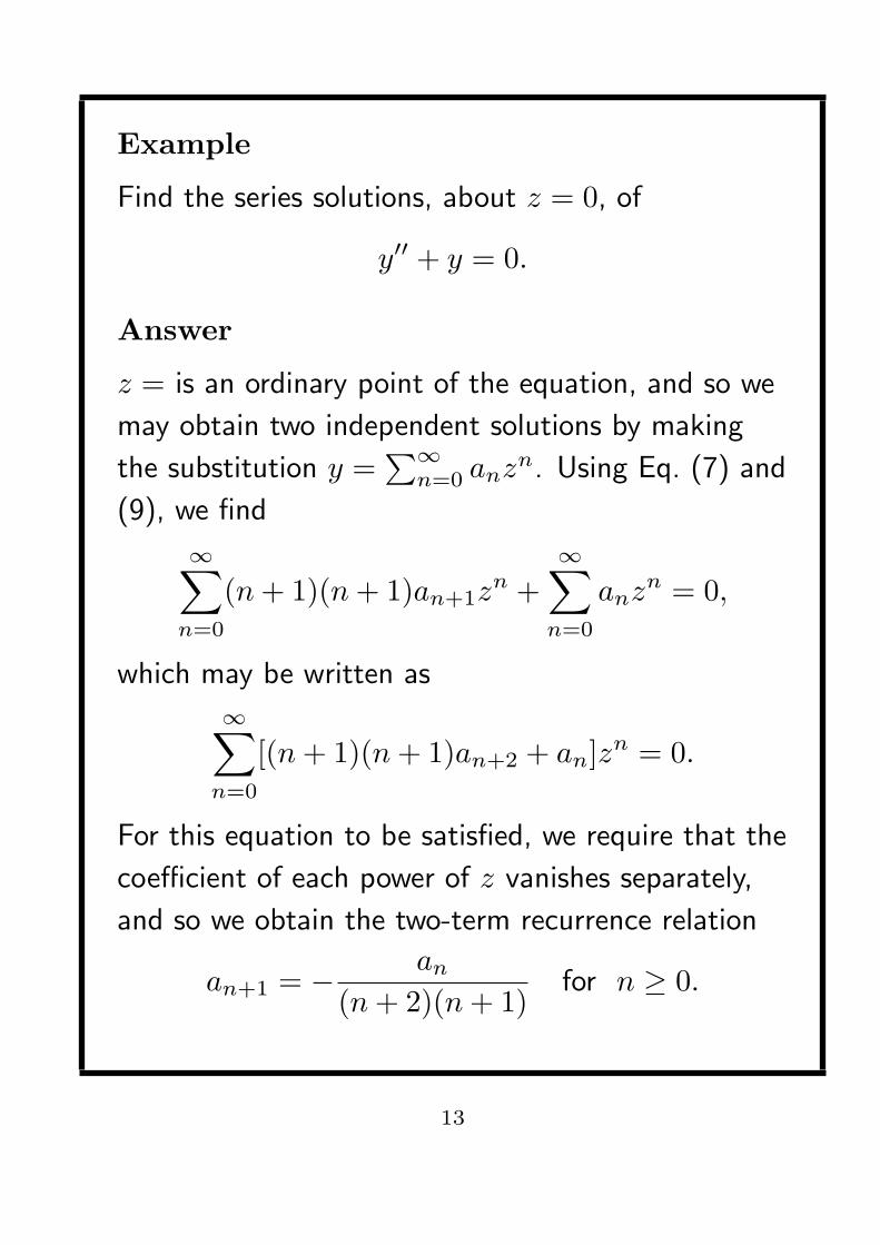
Example
Find the series solutions, about z = 0, of
y′′ + y = 0.
Answer
z = is an ordinary point of the equation, and so we
may obtain two independent solutions by making
the substitution y =∑∞
n=0 anzn. Using Eq. (7) and
(9), we find
∞∑n=0
(n + 1)(n + 1)an+1zn +
∞∑n=0
anzn = 0,
which may be written as
∞∑n=0
[(n + 1)(n + 1)an+2 + an]zn = 0.
For this equation to be satisfied, we require that the
coefficient of each power of z vanishes separately,
and so we obtain the two-term recurrence relation
an+1 = − an
(n + 2)(n + 1)for n ≥ 0.
13

Two independent solutions of the ODE may be
obtained by setting either a0 = 0 or a1 = 0. If we
first set a1 = 0 and choose a0 = 1, then we obtain
the solution
y1(z) = 1− z2
2!+
z4
4!− · · · =
∞∑n=0
(−1)n
(2n)!z2n.
However, if we set a0 = 0 and choose a1 = 1, we
obtain a second independent solution
y2(z) = z − z3
3!+
z5
5!− · · · =
∞∑n=0
(−1)n
(2n + 1)!z2n+1.
Recognizing these two series as cos z and sin z, we
can write the general solution as
y(z) = c1 cos z + c2 sin z,
where c1 and c2 are arbitrary constants.
14

Example
Find the series solutions, about z = 0, of
y′′ − 2(1− z)2
y = 0.
Answer
z = 0 is an ordinary point, and we may therefore
find two independent solutions by substituting
y =∑∞
n=0 anzn. Using Eq. (8) and (9), and
multiplying through by (1− z)2, we find
(1− 2z + z2)∞∑
n=0
n(n− 1)anzn−2 − 2∞∑
n=0
anzn = 0,
which leads to
∞∑n=0
n(n− 1)anzn−2 − 2∞∑
n=0
n(n− 1)anzn−1
+∞∑
n=0
n(n− 1)anzn − 2∞∑
n=0
anzn = 0.
15

In order to write all these series in terms of the
coefficients of zn, we must shift the summation
index in the first two sums to obtain
∞∑n=0
(n + 2)(n + 1)an+2zn − 2
∞∑n=0
(n + 1)nan+1zn
+∞∑
n=0
(n2 − n− 2)anzn = 0,
which can be written as
∞∑n=0
(n+1)[(n+2)an+2−2nan+1+(n−2)an]zn = 0.
By demanding that the coefficients of each power of
z vanish separately, we obtain the recurrence relation
(n + 2)an+2 − 2nan+1 + (n− 2)an = 0 for n ≥ 0,
which determines an for n ≥ 2 in terms of a0 and
a1.
16

One solution has an = a0 for all n, in which case
(choosing a0 = 1), we find
y1(z) = 1 + z + z2 + z3 + · · · = 11− z
.
The other solution to the recurrence relation is
a1 = −2a0, a2 = a0 and an = 0 for n > 2, so that
we obtain a polynomial solution to the ODE:
y2(z) = 1− 2z + z2 = (1− z)2.
The linear independence of y1 and y2 can be
checked:
W = y1y′2 − y′1y2
=1
1− z[−2(1− z)]− 1
(1− z)2(1− z)2 = −3.
The general solution of the ODE is therefore
y(z) =c1
1− z+ c2(1− z)2.
17

Series solutions about a regular singularpoint
If z = 0 is a regular singular point of the equation
y′′ + p(z)y′ + q(z)y = 0,
then p(z) and q(z) are not analytic at z = 0. But
there exists at least one solution to the above
equation, of the form
y = zσ∞∑
n=0
anzn, (10)
where the exponent σ may be real or complex
number, and where a0 6= 0. Such a series is called a
generalized power series or Frobenius series.
18

Since z = 0 is a regular singularity of the ODE,
zp(z) and z2q(z) are analytic at z = 0, so that we
may write
zp(z) = s(z) =∞∑
n=0
snzn
z2q(z) = t(z) =∞∑
n=0
tnzn.
The original ODE therefore becomes
y′′ +s(z)z
y′ +t(z)z2
y = 0.
Let us substitute the Frobenius series Eq. (10) into
this equation. The derivatives of Eq. (10) with
respect to x are given by
y′ =∞∑
n=0
(n + σ)anzn+σ−1 (11)
y′′ =∞∑
n=0
(n + σ)(n + σ − 1)anzn+σ−2, (12)
19

and we obtain
∞∑n=0
(n + σ)(n + σ − 1)anzn+σ−2
+s(z)∞∑
n=0
(n + σ)anzn+σ−2 + t(z)∞∑
n=0
anzn+σ−2 = 0.
Dividing this equation through by zσ−2 we find
∞∑n=0
[(n+σ)(n+σ−1)+s(z)(n+σ)+t(z)]anzn = 0.
(13)Setting z = 0, all terms in the sum with n > 0vanish, so that
[σ(σ − 1) + s(0)σ + t(0)]a0 = 0,
which, since we require a0 6= 0, yields the indicial
equation
σ(σ − 1) + s(0)σ + t(0) = 0. (14)
20

This equation is a quadratic in σ and in general has
two roots. The two roots of the indicial equation σ1
and σ2 are called the indices of the regular singular
point. By substituting each of these roots into
Eq. (13) in turn, and requiring that the coefficients
of each power of z vanish separately, we obtain a
recurrence relation (for each root) expressing each
an as a function of the previous ar (0 ≤ r ≤ n− 1).Depending on the roots of the indicial equation σ1
and σ2, there are three possible general cases.
21
Distinct roots not differing by an integer
If the roots of the indicial equation σ1 and σ2 differ
by an amount that is not an integer, then the
recurrence relations corresponding to each root lead
to two linearly independent solutions of the ODE,
y1(z) = zσ1
∞∑n=0
anzn, y2(z) = zσ2
∞∑n=0
bnzn.
The linear independence of these two solutions
follows from the fact that y2/y1 is not a constant
since σ1 − σ2 is not an integer. Since y1 and y2 are
linearly independent we may use them to construct
the general solution y = c1y1 + c2y2.
We also note that this case includes complex
conjugate roots where σ2 = σ∗1 , since
σ1 − σ2 = σ1 − σ∗1 = 2i Im σ1 cannot be equal to a
real integer.
22
Example
Find the power series solutions about z = 0 of
4zy′′ + 2y′ + y = 0.
Answer
Dividing through by 4z, we obtain
y′′ +12z
y′ +14z
y = 0, (15)
and on comparing with Eq. (5) we identify
p(z) = 1/(2z) and q(z) = 1/(4z). Clearly z = 0 is a
singular point of Eq. (15), but since zp(z) = 1/2and z2q(z) = z/4 are finite there, it is a regular
singular point. We therefore substitute the
Frobenius series y = zσ∑∞
n=0 anzn into Eq. (15).
Using Eq. (11) and (12), we obtain
∞∑n=0
(n + σ)(n + σ − 1)anzn+σ−2
+12z
∞∑n=0
(n + σ)anzn+σ−1 +14z
∞∑n=0
anzn+σ = 0,
23

which on dividing through by zσ−2 gives
∞∑n=0
[(n + σ)(n + σ − 1) +12(n + σ) +
14z]anzn = 0.
(16)If we set z = 0 then all terms in the sum with n > 0vanish, and we obtain the indicial equation
σ(σ − 1) +12σ = 0,
which has roots σ = 1/2 and σ = 0. Since these
roots do not differ by an integer, we expect to find
two independent solutions to Eq. (15), in the form
of Frobenius series.
Demanding that the coefficients of zn vanish
separately in Eq. (16), we obtain the recurrence
relation
(n+σ)(n+σ−1)an+12(n+σ)an+
14an−1 = 0. (17)
24

If we choose the larger root of the indicial equation,
σ = 1/2, this becomes
(4n2 + 2n)an + an−1 = 0 ⇒ an =−an−1
2n(2n + 1).
Setting a0 = 1 we find an = (−1)n/(2n + 1)! and
so the solution to Eq. (15) is
y1(z) =√
z∞∑
n=0
(−1)n
(2n + 1)!zn
=√
z − (√
z)3
3!+
(√
z)5
5!− · · · = sin
√z.
To obtain the second solution, we set σ = 0 in
Eq. (17), which gives
(4n2 − 2n)an + an−1 = 0 ⇒ an = − an−1
2n(2n− 1).
Setting a0 = 1 now gives an = (−1)n/(2n)!, and so
the second solution to Eq. (15) is
y2(z) =∞∑
n=0
(−1)n
(2n)!zn
= 1− (√
z)2
2!+
(√
z)4
4!− · · · = cos
√z.
25

We may check that y1(z) and y2(z) are linearly
independent by computing the Wronskian
W = y1y′2 − y2y
′1
= sin√
z
(− 1
2√
zsin√
z
)
− cos√
z
(1
2√
zcos
√z
)
= − 12√
z(sin2√z + cos2
√z)
= − 12√
z6= 0.
Since W 6= 0 the solutions y − 1(z) and y2(z) are
linearly independent. Hence the general solution to
Eq. (15) is given by
y(z) = c1 sin√
z + c2 cos√
z.
26

Repeated root of the indicial equation
If the indicial equation has a repeated root, so that
σ1 = σ2 = σ, then only one solution in the form of
a Frobenius series Eq. (10) may be found
y1(z) = zσ∞∑
n=0
anzn.
27

Distinct roots differing by an integer
If the roots of the indicial equation differ by an
integer, then the recurrence relation corresponding
to the larger of the two roots leads to a solution of
the ODE. For complex roots, the ‘larger’ root is
taken to be the one with the larger real part.
28

Example
Find the power series solutions about z = 0 of
z(z − 1)y′′ + 3zy′ + y = 0. (18)
Answer
Dividing through by z(z − 1), we put
y′′ +3
(z − 1)y′ +
1z(z − 1)
y = 0, (19)
and on comparing with Eq. (5), we identify
p(z) = 3/(z − 1) and q(z) = 1/[z(z − 1)]. We see
that z = 0 is a singular point of Eq. (19), but since
zp(z) = 3z/(z − 1) and z2q(z) = z/(z − 1) are
finite there, it is a regular singular point. We
substitute y = zσ∑∞
n=0 anzn into Eq. (19), and
using Eq. (11) and (12), we obtain
29

∞∑n=0
(n + σ)(n + σ − 1)anzn+σ−2
+3
z − 1
∞∑n=0
(n + σ)anzn+σ−1
+1
z(z − 1)
∞∑n=0
anzn+σ = 0,
which on dividing through by zσ−2 gives
∞∑n=0
[(n + σ)(n + σ − 1) +
3z
z − 1(n + σ)
+z
z − 1
]anzn = 0.
Multiplying through by z − 1, we obtain
∞∑n=0
[(z−1)(n+σ)(n+σ−1)+3z(n+σ)+z]anzn = 0.
(20)
30

If we set z = 0, then all terms in the sum with
n > 0 vanish, and we obtain the indicial eqaution
σ(σ − 1) = 0,
which has the roots σ = 1 and σ = 0.
Since the roots differ by an integer, it may not be
possible to find two linearly independent solutions of
Eq. (19) in the form of Frobenius series. We are
guaranteed to find one such solution corresponding
to the larger root, σ = 1.
Demanding that the coefficients of zn vanish
separately in Eq. (20), we obtain the recurrence
relation
(n− 1 + σ)(n− 2 + σ)an−1 − (n + σ)(n + σ − 1)an
+3(n− 1 + σ)an−1 + an−1 = 0,
which may be simplified to give
(n + σ − 1)an = (n + σ)an−1. (21)
31

Substituting σ = 1 into this expression, we obtain
an =(
n + 1n
)an−1,
and setting a0 = 1 we find an = n + 1, so one
solution to Eq. (19) is
y1(z) = z∞∑
n=0
(n + 1)zn = z(1 + 2z + 3z2 + · · ·)
=z
(1− z)2. (22)
If we attempt to find a second solution
(corresponding to the smaller root of the indicial
equation) by setting σ = 0 in Eq. (21), we find
an =(
n
n− 1
)an−1,
but we require a0 6= 0, so a1 is formally infinite and
the method fails.
32

Obtaining a second solution
The Wronskian method
If y1 and y2 are linearly independent solutions of the
standard equation
y′′ + p(z)y′ + q(z)y = 0,
then the Wronskian of these two solutions is given
by W (x) = y1y′2 − y2y
′1. Dividing the Wronskian by
y21 we obtain
W
y21
=y′2y1− y′1
y21
y2
=y′2y1
+[
d
dz
(1y1
)]y2 =
d
dz
(y2
y1
),
which integrates to give
y2(x) = y1(x)∫ x W (u)
y21(u)
du.
33

Using the alternative expression for W (z) given in
Eq. (4) with C = 1, we find
y2(z) = y1(z)∫ z 1
y21(u)
exp{−
∫ u
p(v) dv
}du.
(23)Hence, given y1, we can calculate y2.
34

Example
Find a second solution to Eq. (19) using the
Wronskian method.
Answer
For the ODE Eq. (19) we have p(z) = 3/(z − 1),and from Eq. (22) we see that one solution to
Eq. (19) is y1 = z/(1− z)2. Substituting for p and
y1 in Eq. (23) we have
y2(z) = z(1−z)2
∫ z (1−u)4
u2 exp(− ∫ u 3
v−1dv)
du
= z(1−z)2
∫ z (1−u)4
u2 exp[−3 ln(u− 1)] du
= z(1−z)2
∫ z u−1u2 du
= z(1−z)2
(ln z + 1
z
).
35

The derivative method
The method begins with the derivation of a
recurrence relation for the coefficients an in the
Frobenius series solution. However, rather than
putting σ = σ1 in this recurrence relation to
evaluate the first series solution, we instead keep σ
as a variable parameter. This means that the
computed an are functions of σ and the computed
solution is now a function of z and σ
y(z, σ) = zσ∞∑
n=0
an(σ)zn. (24)
Let
L =d2
dx2+ p(z)
d
dx+ q(z),
The series Ly(z, σ) will contain only a term in zσ,
since the recurrence relation defining the an(σ) is
such that these coefficients vanish for higher powers
of z. But the coefficients of zσ is simply the LHS of
the indicial equation.
36

Therefore, if the roots of the indicial equation are
σ = σ1 and σ = σ2, it follows that
Ly(z, σ) = a0(σ − σ1)(σ − σ2)zσ. (25)
Thus, for y(z, σ) to be a solution of the ODE
Ly = 0, σ must equal σ1 or σ2. For simplicity, we
shall set a0 = 1 in the following discussion.
Let us first consider the case in which the two roots
of the indicial equation are equal, σ1 = σ2. From
Eq. (25) we then have
Ly(z, σ) = (σ − σ1)2zn.
Differentiating this equation with respect to σ, we
obtain
∂
∂σ[Ly(z, σ)] = (σ − σ1)2zσ ln z + 2(σ − σ1)zσ,
which equal zero if σ = σ1. But since ∂/∂σ and Lare operators that differentiate with respect to
different variables, we can reverse their order, so that
L[
∂
∂σy(z, σ)
]= 0 at σ = σ1.
37
Hence the function in square brackets, evaluated at
σ = σ1, and denoted by[
∂
∂σy(z, σ)
]
σ=σ1
, (26)
is also a solution of the original ODE Ly = 0, and is
the second linearly independent solution.
The case by which the roots of the indicial equation
differ by an integer is now treated. In Eq. (25),
since L differentiates with respect to z we may
multiply Eq. (25) by any function of σ, say σ − σ2,
and take this function inside L on the LHS to obtain
L[(σ − σ2)y(z, σ)] = (σ − σ1)(σ − σ2)2zσ. (27)
Therefore the function
[(σ − σ2)y(z, σ)]σ=σ2
is also a solution of the ODE Ly = 0.
38

Since this function is not linearly independent with
y(z, σ1), we must find another solution.
Differentiating Eq. (27) with respect to σ, we find
∂
∂σ{L[(σ − σ2)y(z, σ)]} = (σ − σ2)2zσ
+2(σ − σ1)(σ − σ2)zσ + (σ − σ1)(σ − σ2)2zσ ln z,
which is equal to zero if σ = σ2. Therefore,
L{
∂
∂σ[(σ − σ2)y(z, σ)]
}= 0 at σ = σ2,
and so the function{
∂
∂σ[(σ − σ2)y(z, σ)]
}
σ=σ2
(28)
is also a solution of the original ODE Ly = 0, and is
the second linearly independent solution.
39

Example
Find a second solution to Eq. (19) using the
derivative method.
Answer
From Eq. (21) the recurrence relation (with σ as a
parameter) id given by
(n + σ − 1)an = (n + σ)an−1.
Setting a0 = 1 we find that the coefficients have the
particularly simple form an(σ) = (σ + n)/σ. We
therefore consider the function
y(z, σ) = zσ∞∑
n=0
an(σ)zn = zσ∞∑
n=0
σ + n
σzn.
The smaller toot of the indicial equation for
Eq. (19) is σ2 = 0, and so from Eq. (28) a second
linearly independent solution to the ODE is
{∂
∂σ[σy(z, σ)]
}
σ=0
=
{∂
∂σ
[zσ
∞∑n−0
(σ + n)zn
]}
σ=0
.
40
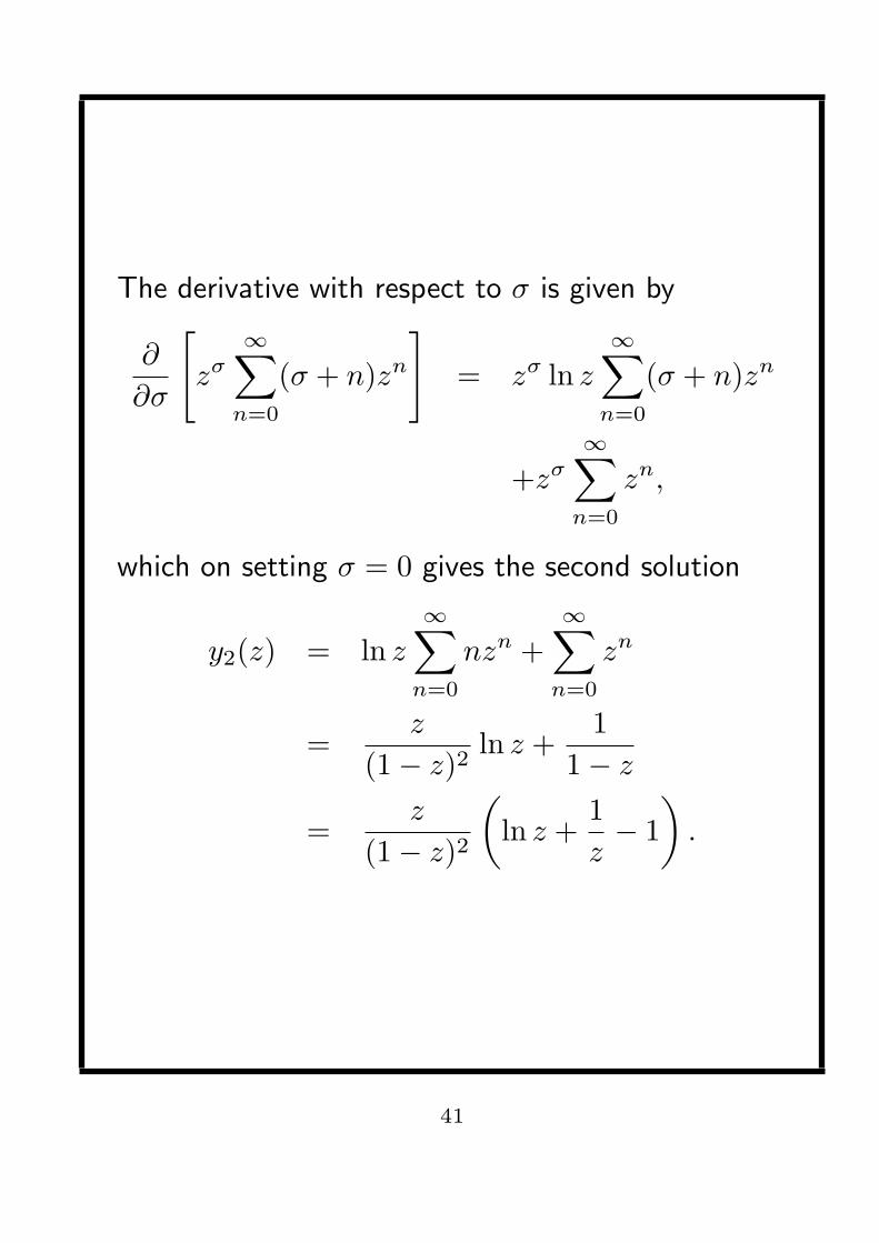
The derivative with respect to σ is given by
∂
∂σ
[zσ
∞∑n=0
(σ + n)zn
]= zσ ln z
∞∑n=0
(σ + n)zn
+zσ∞∑
n=0
zn,
which on setting σ = 0 gives the second solution
y2(z) = ln z∞∑
n=0
nzn +∞∑
n=0
zn
=z
(1− z)2ln z +
11− z
=z
(1− z)2
(ln z +
1z− 1
).
41

Series form of the second solution
Let us consider the case when the two solutions of
the indicial equation are equal. In this case, a
second solution is given by Eq. (26),
y2(z) =[∂y(z, σ)
∂σ
]
σ=σ1
= (ln z)zσ1
∞∑n=0
an(σ1)zn
+zσ1
∞∑n=0
[dan(σ)
dσ
]
σ=σ1
zn
= y1(z) ln z + zσ1
∞∑n=1
bnzn,
where bn = [dan(σ)/dσ]σ=σ1 .
42

In the case where the roots of the indicial equation
differ by an integer, then from Eq. (28) a second
solution is given by
y2(z) ={
∂
∂σ[(σ − σ2)y(z, σ)]
}
σ=σ2
= ln z
[(σ − σ2)zσ
∞∑n=0
an(σ)zn
]
σ=σ2
+zσ2∑n=0
[d
dσ(σ − σ2)an(σ)
]
σ=σ2
zn.
But (σ − σ2)y(z, σ)] at σ = σ2 is just a multiple of
the first solution y(z, σ1). Therefore the second
solution is of the form
y2(z) = cy1(z) ln z + zσ2
∞∑n=0
bnzn,
where c is a constant.
43

Polynomial solutions
Example
Find the power series solutions about z = 0 of
y′′ − 2zy′ + λy = 0. (29)
For what values of λ does the equation possess a
polynomial solution? Find such a solution for λ = 4.
Answer
z = 0 is an ordinary point of Eq. (29) and so we
look for solutions of the form y =∑∞
n=0 znzn.
Substituting this into the ODE and multiplying
through by z2, we find
∞∑n=0
[n(n− 1)− 2z2n + λz2]anzn = 0.
44

By demanding that the coefficients of each power of
z vanish separately we derive the recurrence relation
n(n− 1)an − 2(n− 2)an−2 + λan−2 = 0,
which may be rearranged to give
an =2(n− 2)− λ
n(n− 1)an−2 for n ≥ 2. (30)
The odd and even coefficients are therefore
independent of one another, and two solutions to
Eq. (29) may be derived. We sither set a1 = 0 and
a0 = 1 to obtain
y1(z) = 1−λz2
2!−λ(4−λ)
z4
4!−λ(4−λ)(8−λ)
z6
6!−· · · ,(31)
or set a0 = 0 and a1 = 1 to obtain
y2(z) = z − (2− λ)z3
3!− (2− λ)(6− λ)
z5
5!
−(2− λ)(6− λ)(10− λ)z7
7!− · · · .
45

Now from the recurrence relation Eq. (30) we see
that for the ODE to possess a polynomial solution
we require λ = 2(n− 2) for n ≥ 2, or more simply
λ = 2n for n ≥ 0, i.e. λ must be an even positive
integer. If λ = 4 then from Eq. (31) the ODE has
the polynomial solution
y1(z) = 1− 4z2
2!= 1− 2z2.
ALTERNATIVE SOLUTION:
We assume a polynomial solution to Eq. (29) of the
form y =∑N
n=0 anzn. Substituting this form into
Eq. (29) we find
∞∑n=0
[n(n− 1)anzn−2 − 2znanzn−1 + λnanzn] = 0.
Starting with the highest power of z, we demand
that the coefficient of zN vanishes. We require
−2N + λ = 0 or λ = 2N .
46

Legendre’s equation
Legendre’s equation is
(1− z2)y′′ − 2zy′ + l(l + 1)y = 0. (32)
In normal usage, the variable z is the cosine of the
polar angle in spherical polars, and thus −1 ≤ z ≤ 1.
The parameter l is a given real number, and any
solution of Eq. (32) is called a Legendre function.
z = 0 is an ordinary point of Eq. (32), and so there
are two linearly independent solutions of the form
y =∑∞
n=0 anzn. Substituting we find
∞∑n=0
[n(n− 1)anzn−2 − n(n− 1)anzn
−2nanzn + l(l + 1)anzn] = 0,
which on collecting terms gives
∞∑n=0
{(n + 2)(n + 1)an+2
−[n(n + 1)− l(l + 1)]an}zn = 0.
47

The recurrence relation is therefore
an+2 =[n(n + 1)− l(l + 1)]
(n + 1)(n + 2)an, (33)
for n = 0, 1, 2, . . .. If we choose a0 = 1 and a1 = 0then we obtain the solution
y1(z) = 1− l(l + 1)z2
2!
+(l − 2)l(l + 1)(l + 3)z4
4!− · · · ,(34)
whereas choosing a0 = 0 and a1 = 1, we find a
second solution
y2(z) = z − (l − 1)(l + 2)z3
3!
+(l − 3)(l − 1)(l + 2)(l + 4)z5
5!− · · · .
(35)
Both series converge for |z| < 1, so their radius of
convergence is unity. Since Eq. (34) contains only
even powers of z and (35) only odd powers, we can
write the general solution to Eq. (32) as
y = c1y1 + c2y2 for |z| < 1.
48

General solution for integer l
Now, if l is an integer in Eq. (32), i.e. l = 0, 1, 2, . . .
then the recurrence relation Eq. (33) gives
al+2 =[l(l + 1)− l(l + 1)]
(l + 1)(l + 2)al = 0,
so that the series terminates and we obtain a
polynomial solution of order l. These solutions are
called Legendre polynomial of order l; they are
written Pl(z) and are valid for all finite z. It is
convenient to normalize Pl(z) in such a way that
Pl(1) = 1, and as a consequence Pl(−1) = (−1)l.
The first few Legendre polynomials are given by
P0(z) = 1 P1(z) = z
P2(z) =12(3z2 − 1) P3(z) =
12(5z3 − 3z)
P4(z) =18(35z4 − 30z2 + 3)
P5(z) =18(63z5 − 70z3
+15z).
49

According to whether l is an even or odd integer
respectively, either y1(z) in Eq. (34) or y2(z) in
Eq. (35) terminates to give a multiple of the
corresponding Legendre polynomial Pl(z). In either
case, however, the other series does not terminate
and therefore converges only for |z| < 1. According
to whether l is even or odd we define Legendre
function of the second kind as Ql(z) = αly2(z) or
Ql(z) = βly1(z) respectively, where the constants αl
and βl are conventionally taken to have the values
αl =(−1)l/22l[(l/2)!]2
l!for l even, (36)
βl =(−1)(l+1)/22l−1{[(l − 1)/2]!}2
l!for l odd.
(37)
50

These normalization factors are chosen so that the
Ql(z) obey the same recurrence relations as the
Pl(z). The general solution of Legendre’s equation
for integer l is therefore
y(z) = c1Pl(z) + c2Ql(z), (38)
where Pl(z) is a polynomial of order l and so
converges for all z, and Ql(z) is an infinite series
that converges only for |z| < 1.
51

Example
Use the Wronskian method to find a closed-form
expression for Q0(z).
Answer
From Eq. (23) a second solution to Legendre’s
equation Eq. (32), with l = 0, is
y2(z) = P0(z)∫ z 1
[P0(u)]2exp
(∫ u 2v
1− v2dv
)du
=∫ z
exp[− ln(1− u2)
]du
=∫ z du
(1− u2)=
12
ln(
1 + z
1− z
). (39)
Expanding the logarithm in Eq. (39) as a Maclaurin
series we obtain
y2(z) = z +z3
3+
z5
5+ · · · .
52

Comparing this with the expression for Q0(z), using
Eq. (35) with l = 0 and the normalization Eq. (36),
we find that y2(z) is already correctly normalized,
and so
Q0(z) =12
ln(
1 + z
1− z
).
53

Properties of Legendre polynomials
Rodrigues’ formula
Rodrigues’ formula for the Pl(z) is
Pl(z) =1
2ll!dl
dzl(z2 − 1)l. (40)
To prove that this is a representation, we let
u = (z2 − 1)l, so that u′ = 2lz(z2 − 1)l−1 and
(z2 − 1)u′ − 2lzu = 0.
If we differentiate this expression l + 1 times using
Leibnitz’ theorem, we obtain[(z2 − 1)u(l+2) + 2z(l + 1)u(l+1) + l(l + 1)u(l)
]
−2l[zu(l+1) + (l + 1)u(l)
]= 0,
which reduces to
(z2 − 1)u(l+2) + 2zu(l+1) − l(l + 1)u(l) = 0.
54

Changing the sign all through, and comparing the
resulting expression with Legendre’s equation
Eq. (32), we see that u(l) satisfies the same
equation as Pl(z), so that
u(l)(z) = clPl(z), (41)
for some constant cl that depends on l. To establish
the value of cl, we note that the only term in the
expression for the lth derivative of (z2 − 1)l that
does not contain a factor z2 − 1, and therefore does
not vanish at z = 1, is (2z)ll!(z2 − 1)0. Putting
z = 1 in Eq. (41) therefore shows that cl = 2ll!,thus completing the proof of Eq. (40).
55

Example
Use Rodrigues’ formula to show that
Il =∫ 1
−1
Pl(z)Pl(z) dz =2
2l + 1. (42)
Answer
This is obvious for l = 0, and so we assume l ≥ 1.
Then, by Rodrigues’ formula
Il =1
22l(l!)2
∫ 1
−1
[dl(z2 − 1)l
dzl
] [dl(z2 − 1)l
dzl
]dz.
Repeated integration by parts, with all boundary
terms vanishing, reduces this to
Il =(−1)l
22l(l!)2
∫ 1
−1
(z2 − 1)l d2l
dz2l(z2 − 1)l dz
=(2l)!
22l(l!)2
∫ 1
−1
(1− z2)l dz.
56

If we write
Kl =∫ 1
−1
(1− z2)l dz,
then integration by parts (taking a factor 1 as the
second part) gives
Kl =∫ 1
−1
2lz2(1− z2)l−1dz.
Writing 2lz2 as 2l − 2l(1− z2) we obtain
Kl = 2l
∫ 1
−1
(1− z2)l−1dz − 2l
∫ 1
−1
(1− z2)l dz,
= 2lKl−1 − 2lKl
and hence the recurrence relation
(2l + 1)Kl = 2lKl−1. We therefore find
Kl =2l
2l + 12l − 22l − 1
· · · 23K0
= 2ll!2ll!
(2l + 1)!2 =
22l+1(l!)2
(2l + 1)!.
57

Another property of the Pl(z) is their mutual
orthogonality
∫ 1
−1
Pl(z)Pk(z) dz = 0 if l 6= k. (43)
58

Generating function for Legendrepolynomials
The generating function for, say, a series of
functions fn(z) for n = 0, 1, 2, . . . is a function
G(z, h), containing as well as z a dummy variable h,
such that
G(z, h) =∞∑
n=0
fn(z)hn,
i.e. fn(z) is the coefficient of hn in the expansion of
G in powers of h.
Let us consider the functions Pn(z) defined by the
equation
G(z, h) = (1−2zh+h2)−1/2 =∞∑
n=0
Pn(z)hn. (44)
The functions so defined are identical to the
Legendre polynomials and the function
(1− 2zh + h2)−1/2 is the generating function for
them.
59

In the following, dPn(z)/dz will be denoted by P ′n.
First, we differentiate the defining equation Eq. (44)
with respect to z to get
h(1− 2zh + h2)−3/2 =∑
P ′nhn. (45)
Also. we differentiate Eq. (44) with respect to h to
yield
(z − h)(1− 2zh + h2)−3/2 =∑
nPnhn−1. (46)
Eq. (45) can be written suing Eq. (44) as
h∑
Pnhn = (1− 2zh + h2)∑
P ′nhn,
and thus equating coefficients of hn+1 we obtain
the recurrence relation
Pn = P ′n+1 − 2zP ′n + P ′n−1. (47)
Eqs. (45) and (46) can be combined as
(z − h)∑
P ′nhn = h∑
nPnhn−1,
from which the coefficient of hn yields a second
recurrence relation
zP ′n − P ′n−1 = nPn. (48)
60

Eliminating P ′n−1 between Eqs. (47) and (48) gives
the further result
(n + 1)Pn = P ′n+1 − zP ′n. (49)
If we now take the result Eq. (49) with n replaced
by n− 1 and add z times Eq. (48) to it, we obtain
(1− z2)P ′n = n(Pn−1 − zPn).
Finally, differentiating both sides with respect to z
and using Eq. (48) again, we find
(1− z2)P ′′n − 2zP ′n = n[(P ′n−1 − zP ′n)− Pn]
= n(−nPn − Pn)
= −n(n + 1)Pn,
and so the Pn defined by Eq. (44) satisfies
Legendre’s equation. It only remains to verify the
normalization. This is easily done at z = 1 when G
becomes
G(1, h) = [(1− h)2]−1/2 = 1 + h + h2 + · · · ,and thus all the Pn so defined have Pn(1) = 1.
61

Bessel’s equation
Bessel’s equation has the form
z2y′′ + zy′ + (z2 − ν2)y = 0, (50)
where the parameter ν is a given number, which we
may take as ≥ 0 with no loss of generality. In
Bessel’s equation, z is usually a multiple of a radial
distance and therefore ranges from 0 to ∞.
Rewriting Eq. (50) we have
y′′ +1zy′ +
(1− ν2
z2
)y = 0. (51)
By inspection z = 0 is a regular singular point;
hence we try a solution of the form
y = zσ∑∞
n=0 anzn. Substituting this into Eq. (51)
and multiplying the resulting equation by z2−σ, we
obtain∞∑
n=0
[(σ + n)(σ + n− 1) + (σ + n)− ν2
]anzn
+∞∑
n=0
anzn+2 = 0,
62

which simplifies to
∞∑n=0
[(σ + n)2 − ν2]anzn +∞∑
n=0
anzn+2 = 0.
Considering coefficients of z0 we obtain the indicial
equation
σ2 − ν2 = 0,
so that σ = ±ν. For coefficients of higher powers of
z we find
[(σ + 1)2 − ν2
]a1 = 0, (52)
[(σ + n)2 − ν2
]an + an−2 = 0 for n ≥ 2.
(53)
Substituting σ = ±ν into Eqs. (52) and (53) we
obtain the recurrence relations
(1± 2ν)a1 = 0, (54)
n(n± 2ν)an + an−2 = 0 for n ≥ 2. (55)
63

General solution for non-integer ν
If ν is a non-integer, then in general the two roots
of the indicial equation, σ1 = ν and σ2 = −ν, will
not differ by an integer, and we may obtain two
linearly independent solutions. Special cases od
arise, however, when ν = m/2 for m = 1, 3, 5, . . .,
and σ1 − σ2 = 2ν = m is an (odd positive) integer.
For such cases, we may always obtain a solution in
the form of Frobenius series corresponding to the
larger root σ1 = ν = m/2. For the smaller root
σ2 = −ν = −m/2, however, we must determine
whether a second Frobenius series solution is
possible by examining the recurrence relation
Eq. (55), which reads
n(n−m)an + an−2 = 0 for n ≥ 2.
Since m is an odd positive integer in this case, we
can use this recurrence relation (starting with
a0 6= 0) to calculate a2, a4, a6, . . .. It is therefore
possible to find a second solution in the form of a
Frobenius series corresponding to the smaller root
σ2.
64
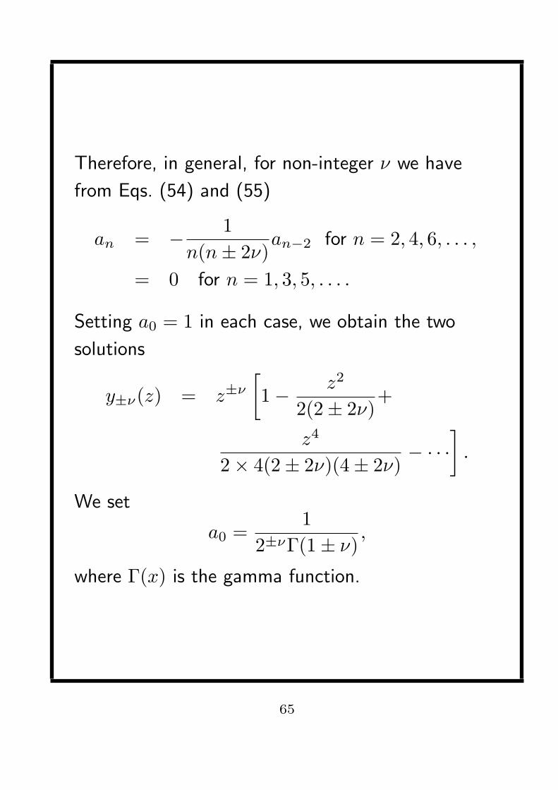
Therefore, in general, for non-integer ν we have
from Eqs. (54) and (55)
an = − 1n(n± 2ν)
an−2 for n = 2, 4, 6, . . . ,
= 0 for n = 1, 3, 5, . . . .
Setting a0 = 1 in each case, we obtain the two
solutions
y±ν(z) = z±ν
[1− z2
2(2± 2ν)+
z4
2× 4(2± 2ν)(4± 2ν)− · · ·
].
We set
a0 =1
2±νΓ(1± ν),
where Γ(x) is the gamma function.
65

The two solutions of Eq. (50) are then written as
Jν(z) and J−ν(z), where
Jν(z) =1
Γ(ν + 1)
(z
2
)ν[1− 1
ν + 1
(z
2
)2
+1
(ν + 1)(ν + 2)12!
(z
2
)4
− · · ·]
=∞∑
n=0
(−1)n
n!Γ(ν + n + 1)
(z
2
)ν+2n
; (56)
and replacing ν by −ν gives J−ν(z). The functions
Jν(z) and J−ν(z) are called Bessel functions of the
first kind, of order ν. Since the first term of each
series is a finite non-zero multiple of zν and z−ν
respectively, if ν is not an integer, Jν(z) and J−ν(z)are linearly independent. Therefore, for non-integer
ν the general solution of Bessel’s equation Eq. (50)
is
y(z) = c1Jν(z) + c2J−ν(z). (57)
66

General solution for integer ν
Let us consider the case when ν = 0, so that the
two solutions to the indicial equation are equal, and
we obtain one solution in the form of a Frobenius
series. From Eq. (56), this is given by
J0(z) =∞∑
n=0
(−1)n22n
22nn!Γ(1 + n)
= 1− z2
22+
z4
2242− z6
224262+ · · · .
In general, however, if ν is a positive integer then
the solutions to the indicial equation differ by an
integer. For the larger root, σ1 = ν, we may find a
solution Jν(z) for ν = 1, 2, 3, . . . , in the form of a
Frobenius series given by Eq. (56).
For the smaller root σ2 = −ν, however, the
recurrence relation Eq. (55) becomes
n(n−m)an + an−2 = 0 for n ≥ 2,
where m = 2ν is now an even positive integer, i.e.
m = 2, 4, 6, . . ..
67

Starting with a0 6= 0, we may calculate
a2, a4, a6, . . ., but we see that when n = m the
coefficient an is infinite, and the method fails to
produce a second solution.
By replacing ν by −ν in the definition of Jν(z),Eq. (56), we have, for integer ν,
J−ν(z) = (−1)νJν(z)
and hence that Jν(z) and J−ν(z) are linearly
dependent. One then defines the function
Yν(z) =Jν(z) cos νπ − J−ν(z)
sin νπ, (58)
which is called a Bessel’s function of the second
kind or order ν. For non-integer ν, Yν(z) is linearly
independent of Jν(z). It may also be shown that
the Wronskian of Jν(z) and Yν(z) is non-zero for all
values of ν. Hence Jν(z) and Yν(z) always
constitute a pair of independent solutions. The
expression Eq. (58) does, however, become an
indeterminate form 0/0 when ν is an integer.
68

This is so because for integer ν we have
cos νπ = (−1)ν and J−ν(z) = (−1)νJν(z). For
integer ν, we set
Yν(z) = limµ→ν
[Jµ(z) cos µπ − J−µ(z)
sin µπ
], (59)
which gives a linearly independent second solution
for integer ν. Therefore, we may write the general
solution of Bessel’s equation, valid for all ν, as
y(z) = c1Jν(z) + c2Yν(z). (60)
69

Properties of Bessel functions
Example
Prove the recurrence relation
d
dz[zνJν(z)] = zνJν−1(z). (61)
Answer
From the power series definition Eq. (56) of Jν(z),we obtain
d
dz[zνJν(z)] =
d
dz
∞∑n=0
(−1)nz2ν+2n
2ν+2nn!Γ(ν + n + 1)
=∞∑
n=0
(−1)nz2ν+2n−1
2ν+2n−1n!Γ(ν + n)
= zν∞∑
n=0
(−1)nz(ν−1)+2n
2(ν−1)+2nn!Γ(ν − 1 + n + 1)
= zνJν−1(z).
70

Similarly, we have
d
dz[z−νJν(z)] = −z−νJν+1(z). (62)
From Eqs. (61) and (62) the remaining recurrence
relations may be derived. Expanding out the
derivative on the LHS of Eq. (61) and dividing
through by zν−1, we obtain the relation
zJ ′ν(z) + νJν(z) = zJν−1(z). (63)
Similarly, by expanding out the derivative on the
LHS of Eq. (62), and multiplying through by zν+1,
we find
zJ ′ν(z)− νJν(z) = −zJν+1(z). (64)
Adding Eq. (63) and Eq. (64) and dividing through
by z gives
Jν−1(z)− Jν+1(z) = 2J ′ν(z). (65)
Finally, subtracting Eq. (64) from Eq. (63) and
dividing through by z gives
Jν−1(z) + Jν+1(z) =2ν
zJν(z). (66)
71

Mutually orthogonality of Bessel functions
By definition, the function Jν(z) satisfies Bessel’s
equation Eq. (50),
z2y′′ + zy′ + (z2 − ν2)y = 0.
Let us instead consider the functions f(z) = Jν(λz)and g(z) = Jν(µz), which respectively satisfy the
equations
z2f ′′ + zf ′ + (λ2z2 − ν2)f = 0, (67)
z2g′′ + zg′ + (µ2z2 − ν2)g = 0. (68)
72

Example
Show that f(z) = Jν(λz) satisfies Eq. (67).
Answer
If f(z) = Jν(λz) and we write w = λz, then
df
dz= λ
dJν(w)dw
andd2f
dz2= λ2 d2Jν(w)
dw2.
When these expressions are substituted, the LHS of
Eq. (67) becomes
z2λ2 d2Jν(w)dw2
+ zλdJν(w)
dw+ (λ2z2 − ν2)Jν(w)
= w2 d2Jν(w)dw2
+ wdJν(w)
dw+ (w2 − ν2)Jν(w).
But, from Bessel’s equation itself, this final
expression is equal to zero, thus verifying that f(z)does satisfy Eq. (67).
73

Now multiplying Eq. (68) by f(z) and Eq. (67) by
g(z) and subtracting gives
d
dz[z(fg′ − gf ′)] = (λ2 − µ2)zfg, (69)
where we have used the fact that
d
dz[z(fg′ − gf ′)] = z(fg′′ − gf ′′) + (fg′ − gf ′).
By integrating Eq. (69) over any given range z = a
to z = b, we obtain
∫ b
a
zf(z)g(z) dz =1
λ2 − µ2[zf(z)g′(z)
−zg(z)f ′(z)]ba ,
which, on setting f(z) = Jν(λz) and
g(z) = Jν(µz), becomes
∫ b
a
zJν(λz)Jν(µz) dz =1
λ2 − µ2[µzJν(λz)J ′ν(µz)
−λzJν(µz)J ′ν(λz)]ba . (70)
74

If λ 6= µ and the interval [a, b] is such that the
expression on the RHS of Eq. (70) equals zero we
obtain the orthogonality condition
∫ b
a
zJν(λz)Jν(µz) dz = 0. (71)
75

Generating function for Bessel functions
The Bessel functions Jν(z), where ν is an integer,
cab be described by a generating function, which is
given by
G(z, h) = exp[z
2
(h− 1
h
)]=
∞∑n=−∞
Jn(z)hn.
(72)By expanding the exponential as a power series, it
can be verified that the functions Jn(z) defined by
Eq. (72) are Bessel functions of the first kind.
76

Example
Use the generating function Eq. (72) to prove, for
integer ν, the recurrence relation Eq. (66), i.e.
Jν−1(z) + Jν+1(z) =2ν
zJν(z).
Answer
Differentiating G(z, h) with respect to h, we obtain
∂G(z, h)∂h
=z
2
(1 +
1h2
)G(z, h) =
∞∑−∞
nJn(z)hn−1,
which can be written using Eq. (72) again as
z
2
(1 +
1h2
) ∞∑−∞
Jn(z)hn =∞∑−∞
nJn(z)hn−1.
Equating coefficients of hn we obtain
z
2[Jn(z) + Jn+2(z)] = (n + 1)Jn+1(z),
which on replacing n by ν − 1 gives the required
recurrence relation.
77


![Discrete difierential geometry. Integrability as consistencypage.math.tu-berlin.de/~bobenko/papers/2004_Bob_p.pdf · difierential geometry see in particular [2], [1]. 2 Origin and](https://img.pdfslide.net/doc/110x75/5f705523e68d005b6865e162/discrete-diierential-geometry-integrability-as-bobenkopapers2004bobppdf.jpg)
![CartanforBeginners: DifierentialGeometryviaMovingFrames ...jml/EDSpublic.pdfx Preface for more advanced texts on exterior difierential systems, such as [20], and papersonrecentadvancesinthetheory,suchas[58,117]](https://img.pdfslide.net/doc/110x75/5e8204c4d8769436eb76e21d/cartanforbeginners-diierentialgeometryviamovingframes-jml-x-preface-for.jpg)