Service Limit State Design for Bridges Background Information on the Proposed Geotechnical Revisions to AASHTO LRFD Naresh C. Samtani, PhD, PE NCS GeoResources, LLC John M. Kulicki, PhD, PE Modjeski and Masters, Inc. October 28, 2015

2

SHRP2 Implementation

51 States + DC

350+ projects

• SHRP2 Solutions – 63 products bundled into 40 implementation efforts

• Solution Development – processes, software, testing procedures, and specifications

• Field Testing – refined in the field

• Implementation – 350+ transportation projects; goal to adopt as standard practice

• SHRP2 Education Connection – connecting next-generation professionals with next-generation innovations

3

Initial SHRP2-TRB Research Team for R19B

• Modjeski and Masters (M&M) – John M. Kulicki (Principal Investigator) – Wagdy G. Wassef (formerly M&M)

• University of Delaware (UD) – Dennis R. Mertz

• University of Nebraska – Lincoln (UNL) – Andrzej S. Nowak (now at Auburn)

• NCS Consultants, LLC (NCS) – Naresh C. Samtani

Report S2-R19B-RW-1

4

Work Under TRB-SHRP2

• General calibration process was developed for SLS and was revised to fit specific requirements for different limit states.

• The following limit states were calibrated: o Fatigue I and Fatigue II limit states for steel components o Fatigue I for compression in concrete and tension in the

reinforcement o Tension in prestressed concrete components o Crack control in decks o Service II limit state for yielding of steel and for bolt slip o Foundation deformation(s)

5

Implementation Tools

• Several examples • White paper • Flow Chart • Proposed LRFD

specification revisions and commentaries

• SHRP2 Round 7 Implementation Assistance Program (IAP)

6

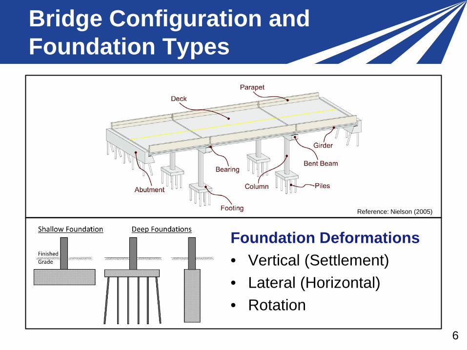
Bridge Configuration and Foundation Types

Foundation Deformations • Vertical (Settlement) • Lateral (Horizontal) • Rotation

Reference: Nielson (2005)

7

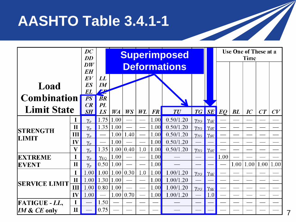
Superimposed Deformations

AASHTO Table 3.4.1-1

8

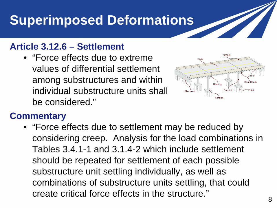
Superimposed Deformations

Article 3.12.6 – Settlement • “Force effects due to extreme

values of differential settlement among substructures and within individual substructure units shall be considered.”

Commentary • “Force effects due to settlement may be reduced by

considering creep. Analysis for the load combinations in Tables 3.4.1-1 and 3.1.4-2 which include settlement should be repeated for settlement of each possible substructure unit settling individually, as well as combinations of substructure units settling, that could create critical force effects in the structure.”

9

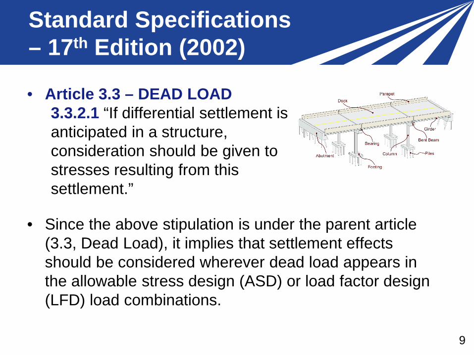
Standard Specifications – 17th Edition (2002)

• Article 3.3 – DEAD LOAD 3.3.2.1 “If differential settlement is anticipated in a structure, consideration should be given to stresses resulting from this settlement.”

• Since the above stipulation is under the parent article (3.3, Dead Load), it implies that settlement effects should be considered wherever dead load appears in the allowable stress design (ASD) or load factor design (LFD) load combinations.

10

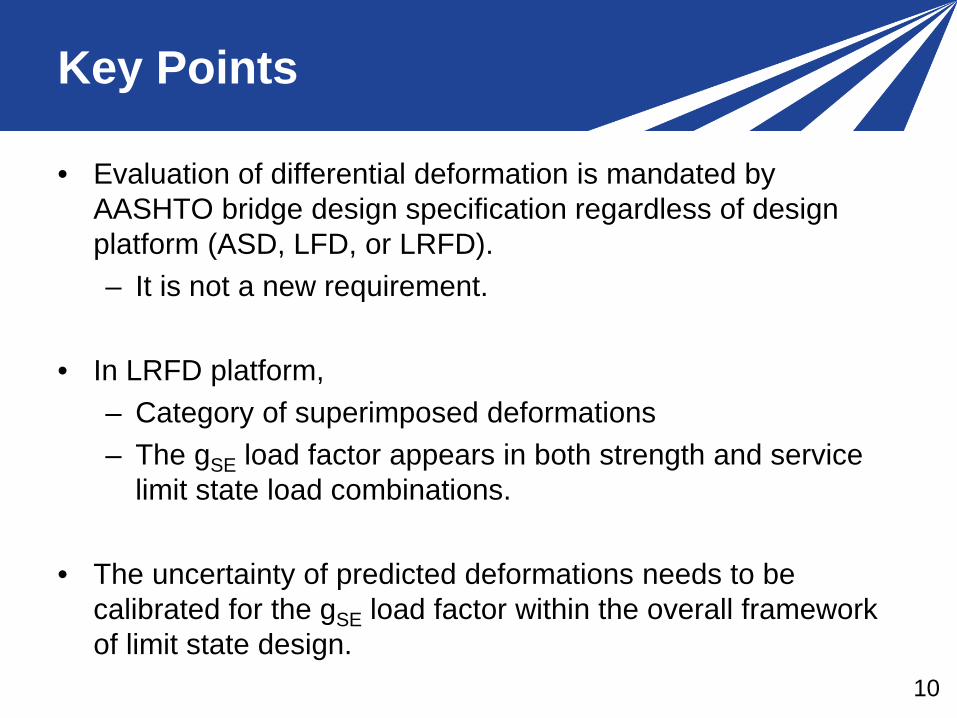
Key Points

• Evaluation of differential deformation is mandated by AASHTO bridge design specification regardless of design platform (ASD, LFD, or LRFD). – It is not a new requirement.

• In LRFD platform,

– Category of superimposed deformations – The gSE load factor appears in both strength and service

limit state load combinations.

• The uncertainty of predicted deformations needs to be calibrated for the gSE load factor within the overall framework of limit state design.

11

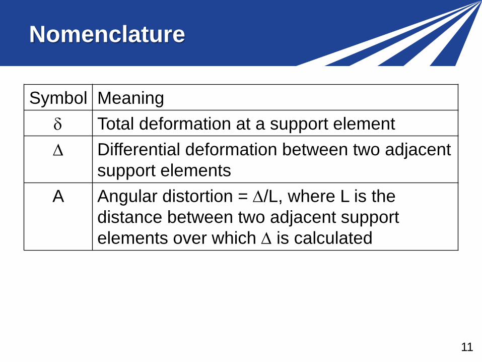
Nomenclature

Symbol Meaning δ Total deformation at a support element ∆ Differential deformation between two adjacent

support elements A Angular distortion = ∆/L, where L is the

distance between two adjacent support elements over which ∆ is calculated

12

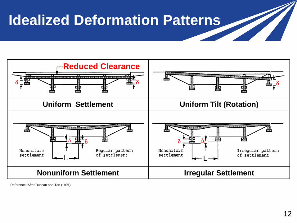
Idealized Deformation Patterns

L Reference: After Duncan and Tan (1991)

Uniform Settlement Uniform Tilt (Rotation)

Nonuniform Settlement Irregular Settlement

L L

∆ ∆ δ δ

δ δ δ

Reduced Clearance

Reference: After Duncan and Tan (1991)

13

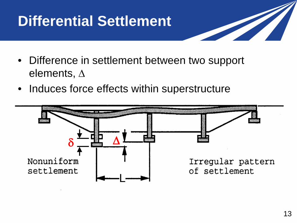
Differential Settlement

• Difference in settlement between two support elements, ∆

• Induces force effects within superstructure

L

∆ δ

14

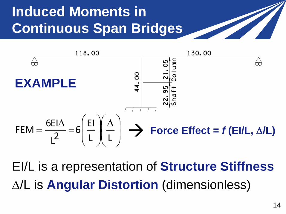
Induced Moments in Continuous Span Bridges

EI/L is a representation of Structure Stiffness ∆/L is Angular Distortion (dimensionless)

∆

=

∆=

LLEI62L

EI6FEM

EXAMPLE

Force Effect = f (EI/L, ∆/L)

15

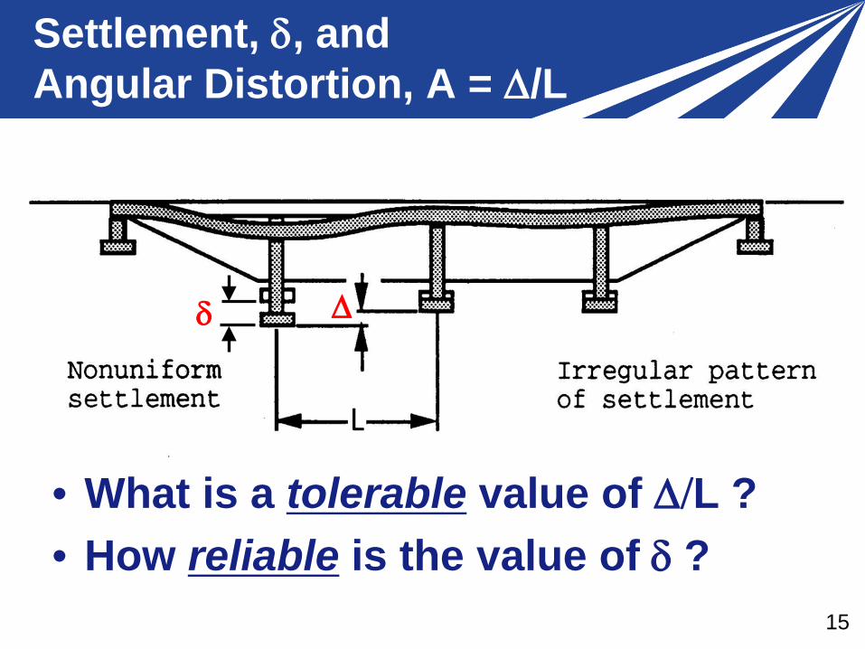
Settlement, δ, and Angular Distortion, A = ∆/L

• What is a tolerable value of ∆/L ? • How reliable is the value of δ ?

∆ δ

16

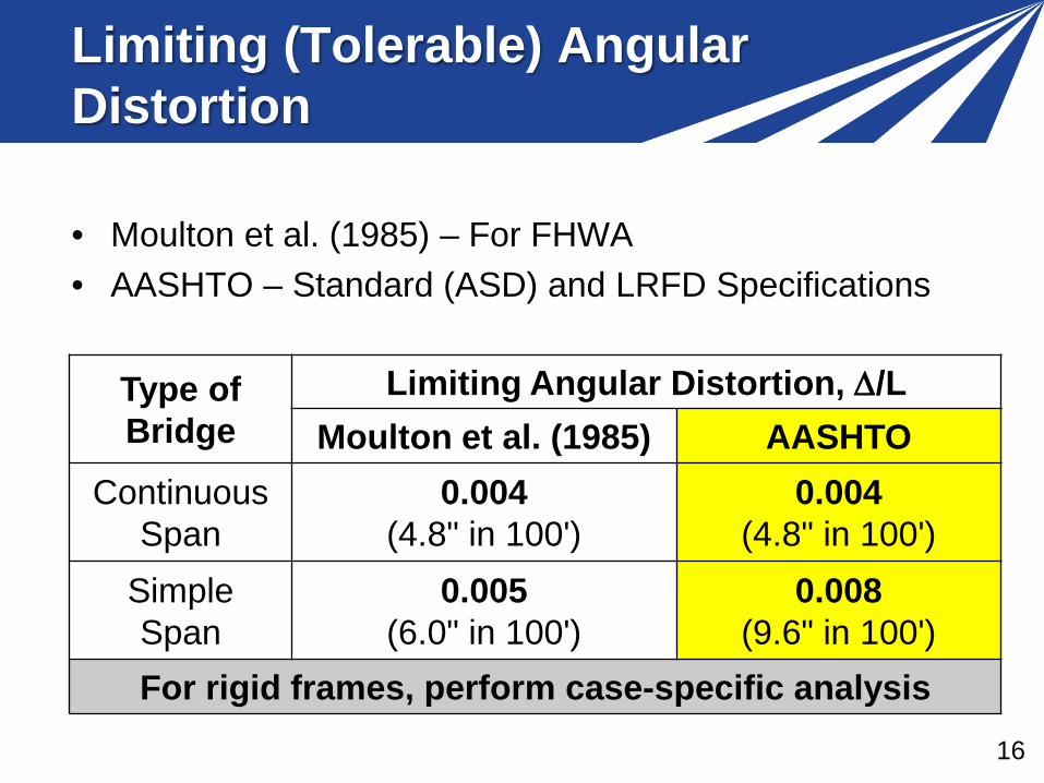
Limiting (Tolerable) Angular Distortion

Type of Bridge

Limiting Angular Distortion, ∆/L Moulton et al. (1985) AASHTO

Continuous Span

0.004 (4.8" in 100')

0.004 (4.8" in 100')

Simple Span

0.005 (6.0" in 100')

0.008 (9.6" in 100')

For rigid frames, perform case-specific analysis

• Moulton et al. (1985) – For FHWA • AASHTO – Standard (ASD) and LRFD Specifications

17

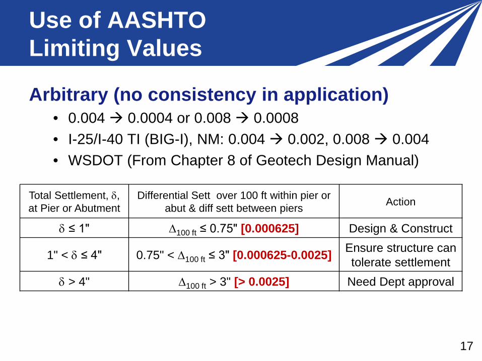
Use of AASHTO Limiting Values

Arbitrary (no consistency in application) • 0.004 0.0004 or 0.008 0.0008 • I-25/I-40 TI (BIG-I), NM: 0.004 0.002, 0.008 0.004 • WSDOT (From Chapter 8 of Geotech Design Manual)

Total Settlement, δ, at Pier or Abutment

Differential Sett over 100 ft within pier or abut & diff sett between piers Action

δ ≤ 1" ∆100 ft ≤ 0.75" [0.000625] Design & Construct

1" < δ ≤ 4" 0.75" < ∆100 ft ≤ 3" [0.000625-0.0025] Ensure structure can tolerate settlement

δ > 4" ∆100 ft > 3" [> 0.0025] Need Dept approval

18

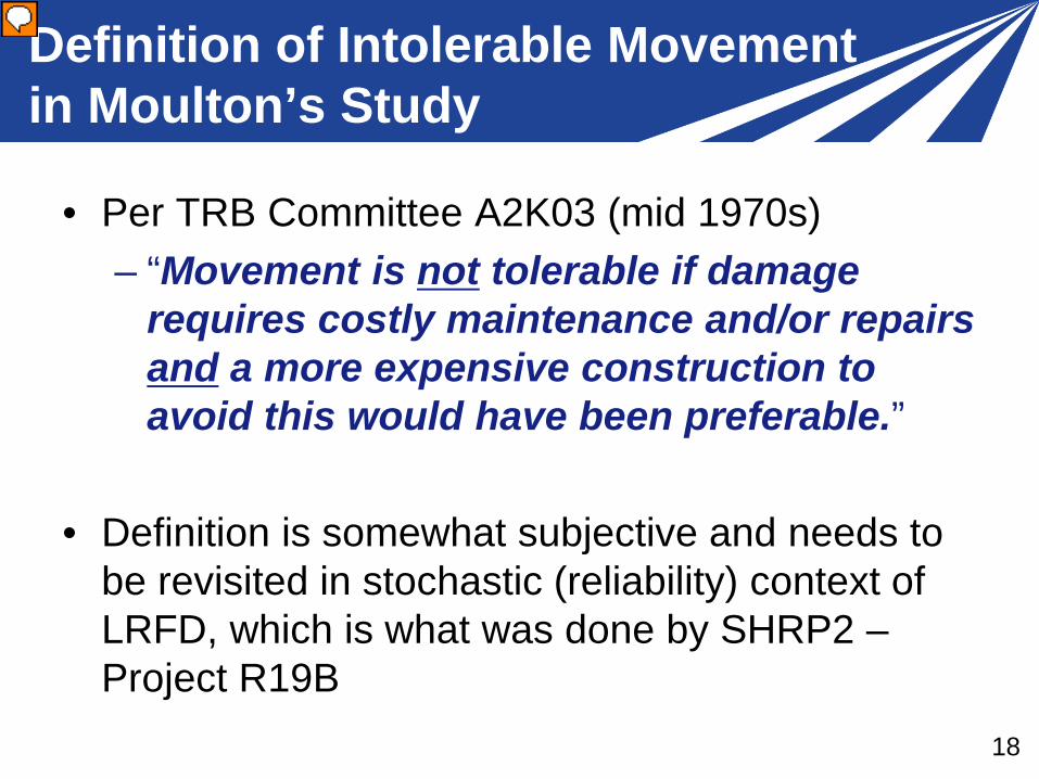
Definition of Intolerable Movement in Moulton’s Study

• Per TRB Committee A2K03 (mid 1970s) – “Movement is not tolerable if damage

requires costly maintenance and/or repairs and a more expensive construction to avoid this would have been preferable.”

• Definition is somewhat subjective and needs to

be revisited in stochastic (reliability) context of LRFD, which is what was done by SHRP2 – Project R19B

19

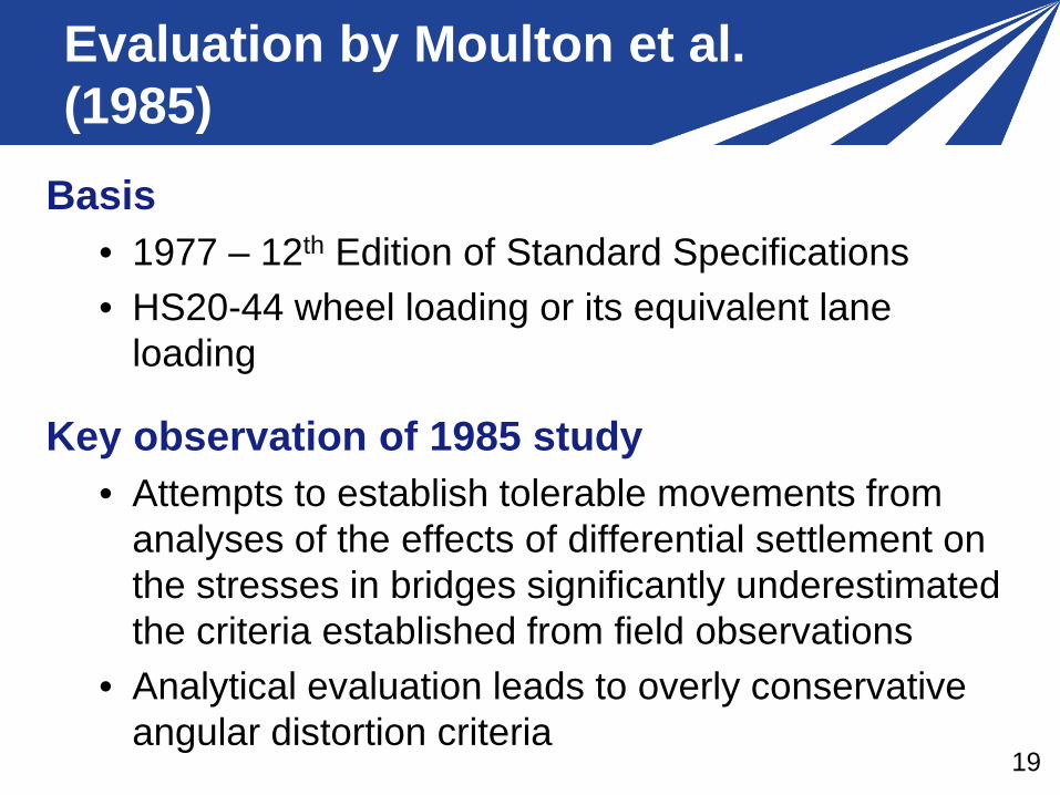
Evaluation by Moulton et al. (1985)

Basis • 1977 – 12th Edition of Standard Specifications • HS20-44 wheel loading or its equivalent lane

loading

Key observation of 1985 study • Attempts to establish tolerable movements from

analyses of the effects of differential settlement on the stresses in bridges significantly underestimated the criteria established from field observations

• Analytical evaluation leads to overly conservative angular distortion criteria

20

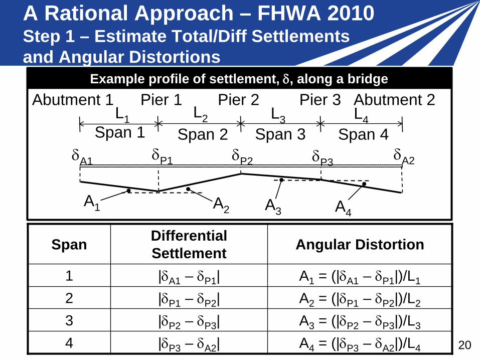
A Rational Approach – FHWA 2010 Step 1 – Estimate Total/Diff Settlements and Angular Distortions

Span Differential Settlement Angular Distortion

1 |δA1 – δP1| A1 = (|δA1 – δP1|)/L1

2 |δP1 – δP2| A2 = (|δP1 – δP2|)/L2

3 |δP2 – δP3| A3 = (|δP2 – δP3|)/L3

4 |δP3 – δA2| A4 = (|δP3 – δA2|)/L4

δA1 δP1 δP2 δP3 δA2

A1 A2 A3 A4

L1 Span 1

L2 Span 2

L3 Span 3

L4 Span 4

Abutment 1 Pier 1 Pier 2 Pier 3 Abutment 2 Example profile of settlement, δ, along a bridge

21

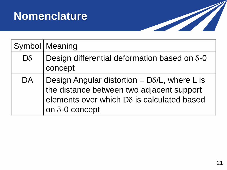
Nomenclature

Symbol Meaning Dδ Design differential deformation based on δ-0

concept DA Design Angular distortion = Dδ/L, where L is

the distance between two adjacent support elements over which Dδ is calculated based on δ-0 concept

22

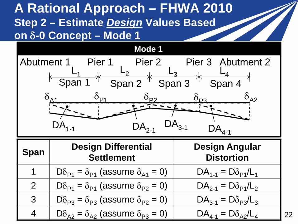
A Rational Approach – FHWA 2010 Step 2 – Estimate Design Values Based on δ-0 Concept – Mode 1

Span Design Differential Settlement

Design Angular Distortion

1 DδP1 = δP1 (assume δA1 = 0) DA1-1 = DδP1/L1

2 DδP1 = δP1 (assume δP2 = 0) DA2-1 = DδP1/L2

3 DδP3 = δP3 (assume δP2 = 0) DA3-1 = DδP3/L3

4 DδA2 = δA2 (assume δP3 = 0) DA4-1 = DδA2/L4

δA1 δP1 δP2 δP3 δA2

DA1-1 DA2-1 DA3-1 DA4-1

L1 Span 1

L2 Span 2

L3 Span 3

L4 Span 4

Abutment 1 Pier 1 Pier 2 Pier 3 Abutment 2 Mode 1

23

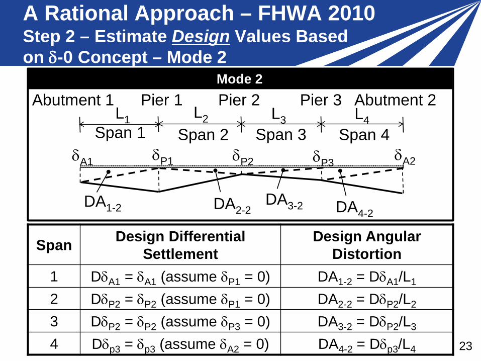
A Rational Approach – FHWA 2010 Step 2 – Estimate Design Values Based on δ-0 Concept – Mode 2

Span Design Differential Settlement

Design Angular Distortion

1 DδA1 = δA1 (assume δP1 = 0) DA1-2 = DδA1/L1

2 DδP2 = δP2 (assume δP1 = 0) DA2-2 = DδP2/L2

3 DδP2 = δP2 (assume δP3 = 0) DA3-2 = DδP2/L3

4 Dδp3 = δp3 (assume δA2 = 0) DA4-2 = Dδp3/L4

δA1 δP1 δP2 δP3 δA2

DA1-2 DA2-2 DA3-2 DA4-2

L1 Span 1

L2 Span 2

L3 Span 3

L4 Span 4

Abutment 1 Pier 1 Pier 2 Pier 3 Abutment 2 Mode 2

24

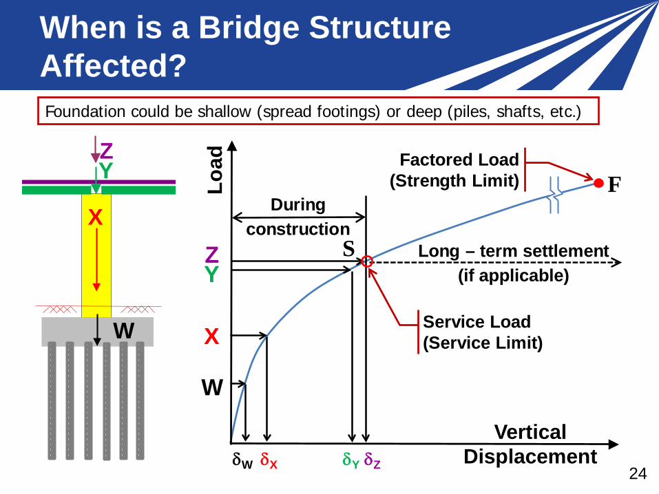
When is a Bridge Structure Affected?

X

Z

Load

Vertical Displacement

Y

W

Long – term settlement (if applicable)

δW δX δY δZ

S

Factored Load (Strength Limit) F

During construction

Service Load (Service Limit)

X

ZY

W

Foundation could be shallow (spread footings) or deep (piles, shafts, etc.)

25

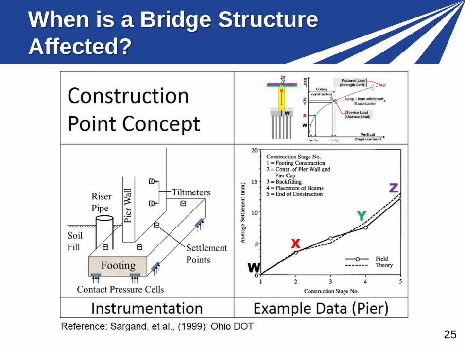
When is a Bridge Structure Affected?

26

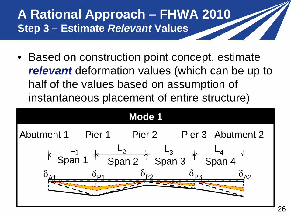
A Rational Approach – FHWA 2010 Step 3 – Estimate Relevant Values

δA1 δP1 δP2 δP3 δA2

L1 Span 1

L2 Span 2

L3 Span 3

L4 Span 4

Abutment 1 Pier 1 Pier 2 Pier 3 Abutment 2

• Based on construction point concept, estimate relevant deformation values (which can be up to half of the values based on assumption of instantaneous placement of entire structure)

Mode 1

27

A Rational Approach – FHWA 2010 Step 3 – Estimate Relevant Values

δA1 δP1 δP2 δP3 δA2

L1 Span 1

L2 Span 2

L3 Span 3

L4 Span 4

Abutment 1 Pier 1 Pier 2 Pier 3 Abutment 2

• Based on construction point concept, estimate relevant deformation values (which can be up to half of the values based on assumption of instantaneous placement of entire structure)

Mode 2

28

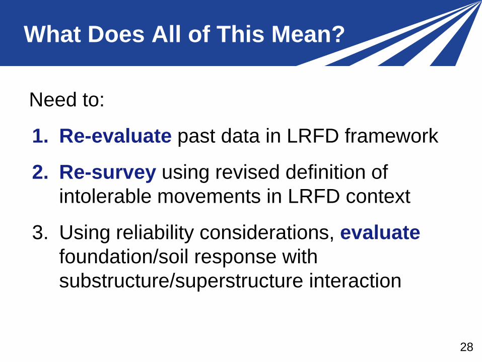
What Does All of This Mean?

Need to:

1. Re-evaluate past data in LRFD framework

2. Re-survey using revised definition of intolerable movements in LRFD context

3. Using reliability considerations, evaluate foundation/soil response with substructure/superstructure interaction

29

Calibration Approach Incorporating reliability into

evaluation of foundation deformations

30

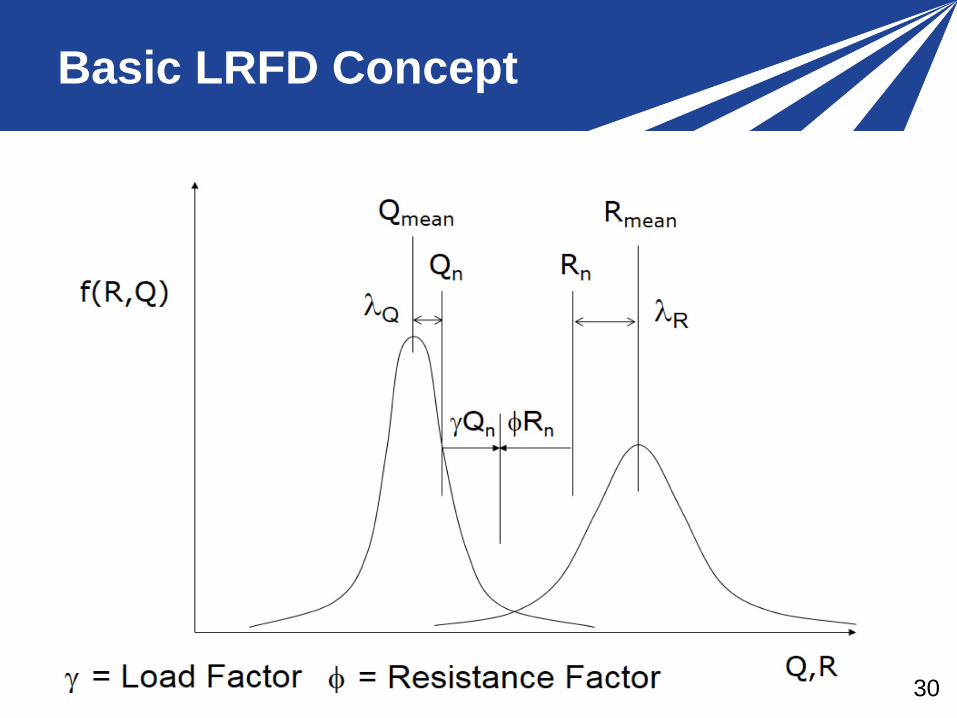
Basic LRFD Concept

31

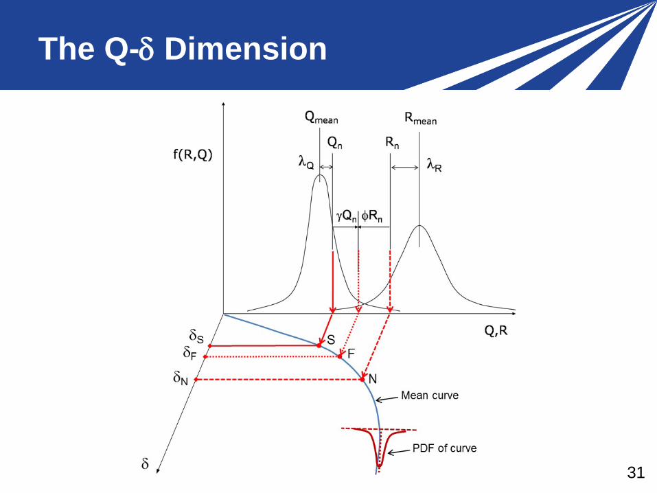
The Q-δ Dimension

32

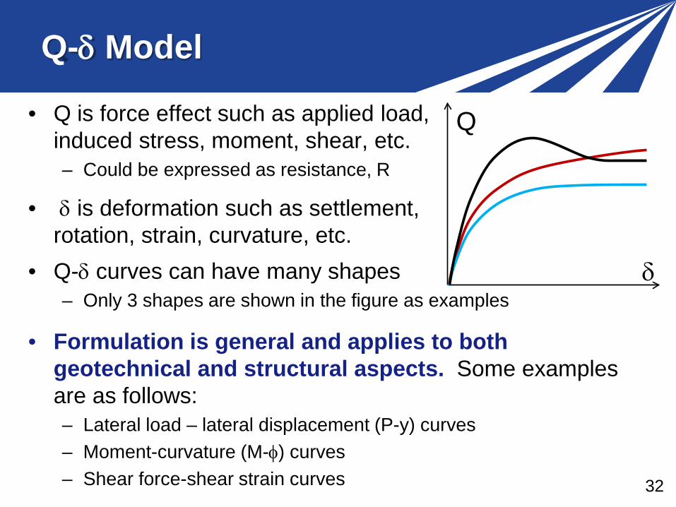
Q-δ Model

• Q is force effect such as applied load, induced stress, moment, shear, etc. – Could be expressed as resistance, R

• δ is deformation such as settlement, rotation, strain, curvature, etc.

Q

δ • Q-δ curves can have many shapes – Only 3 shapes are shown in the figure as examples

• Formulation is general and applies to both geotechnical and structural aspects. Some examples are as follows: – Lateral load – lateral displacement (P-y) curves – Moment-curvature (M-φ) curves – Shear force-shear strain curves

33

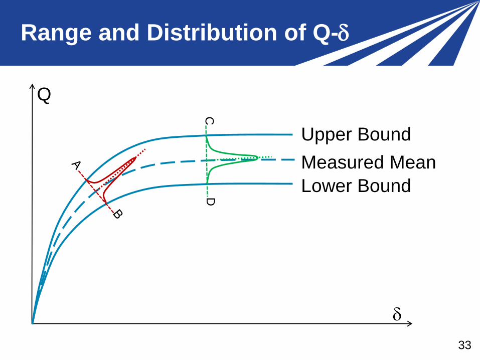
Range and Distribution of Q-δ

Q

δ

Upper Bound

Lower Bound Measured Mean

C

D

34

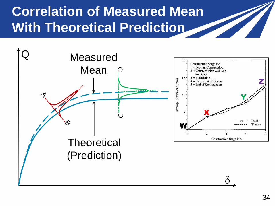
Correlation of Measured Mean With Theoretical Prediction

Q

δ

Theoretical (Prediction)

Measured Mean C

D

35

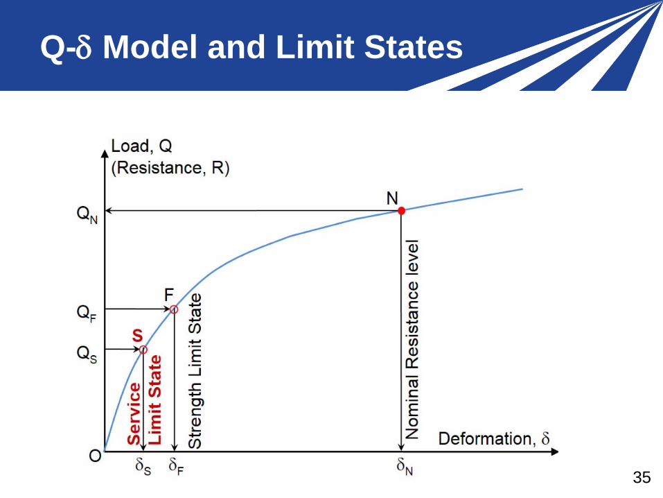
Q-δ Model and Limit States

36

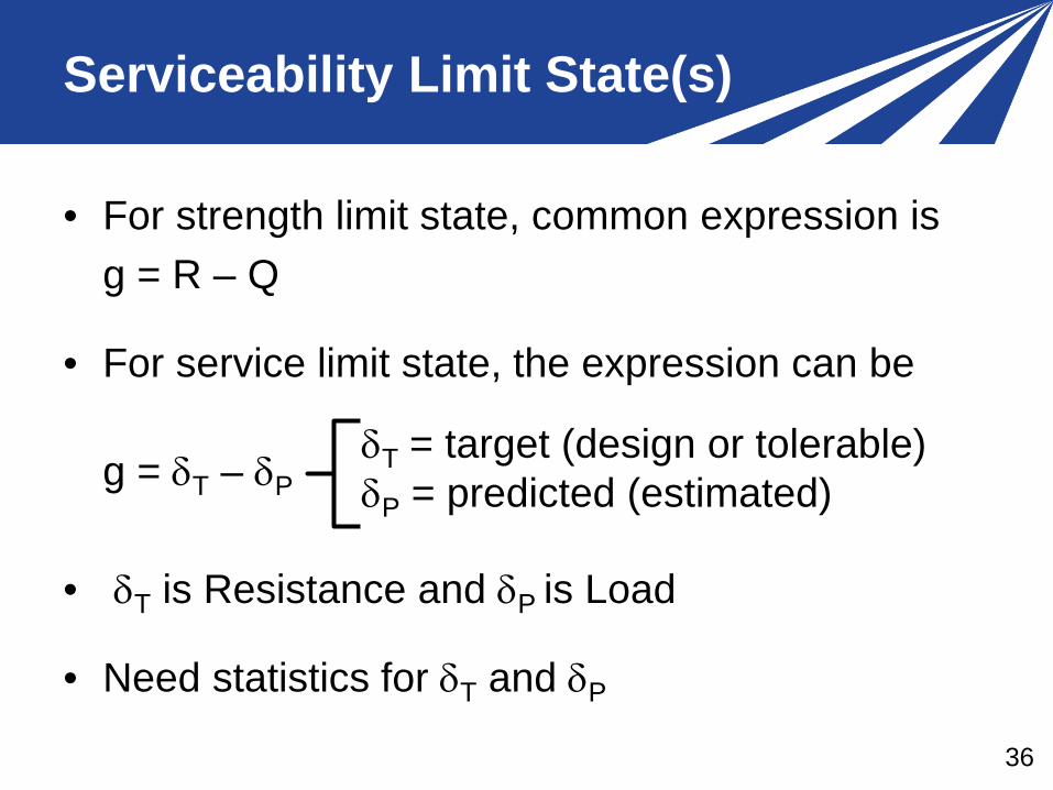
Serviceability Limit State(s)

• For strength limit state, common expression is g = R – Q

• For service limit state, the expression can be g = δT – δP

• δT is Resistance and δP is Load

• Need statistics for δT and δP

δT = target (design or tolerable) δP = predicted (estimated)

37

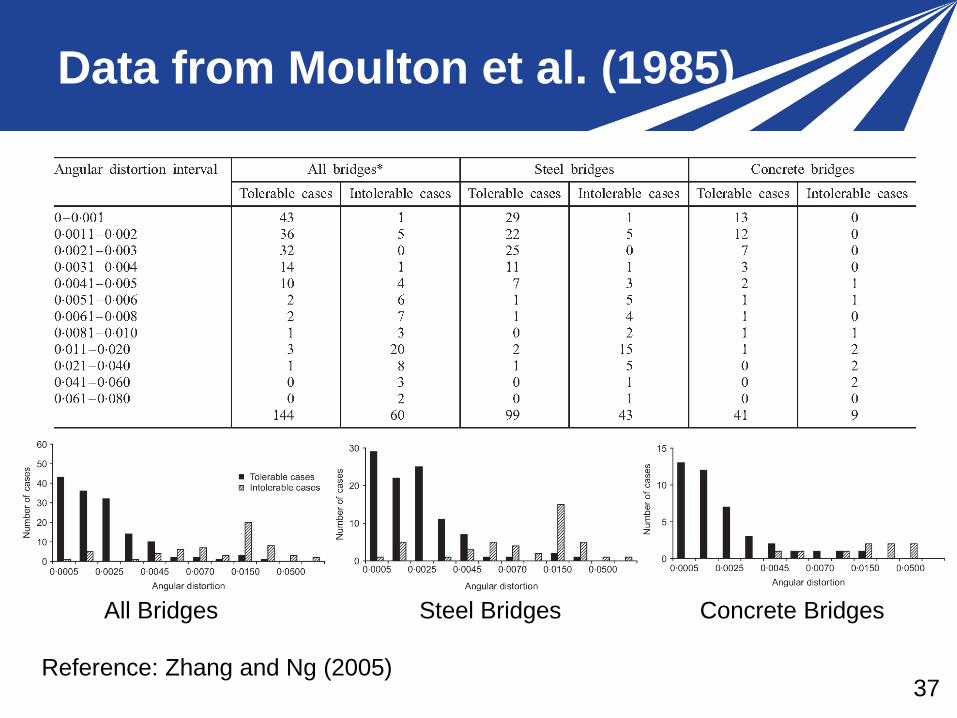
Data from Moulton et al. (1985)

All Bridges Steel Bridges Concrete Bridges

Reference: Zhang and Ng (2005)

38

Statistics for δT (Resistance)

• No consensus on δT

• No standard deviation (σ), Bias (or Accuracy) data available at this time using LRFD specifications – Long Term Bridge Performance Program (LTBPP)

may offer future data

• Use of deterministic value of δT by bridge designer – Varies based on type of bridge structure, joints,

design of specific component, ride quality, deck drainage, aesthetics, public perception, etc.

39

δP

f(R,Q

)

Q,R

δT

Probability of Exceedance, Pe

Adaptations

40

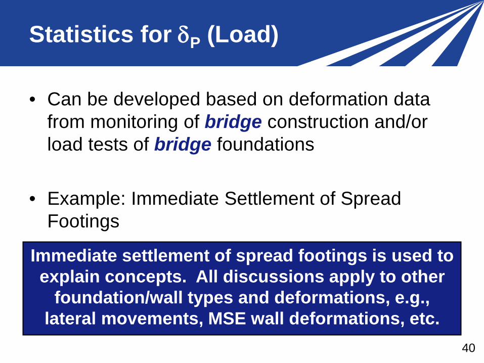
Statistics for δP (Load)

• Can be developed based on deformation data from monitoring of bridge construction and/or load tests of bridge foundations

• Example: Immediate Settlement of Spread Footings

Immediate settlement of spread footings is used to explain concepts. All discussions apply to other

foundation/wall types and deformations, e.g., lateral movements, MSE wall deformations, etc.

41

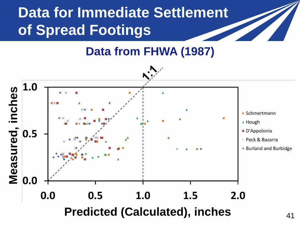
Data for Immediate Settlement of Spread Footings

Predicted (Calculated), inches

Mea

sure

d, in

ches

Data from FHWA (1987)

42

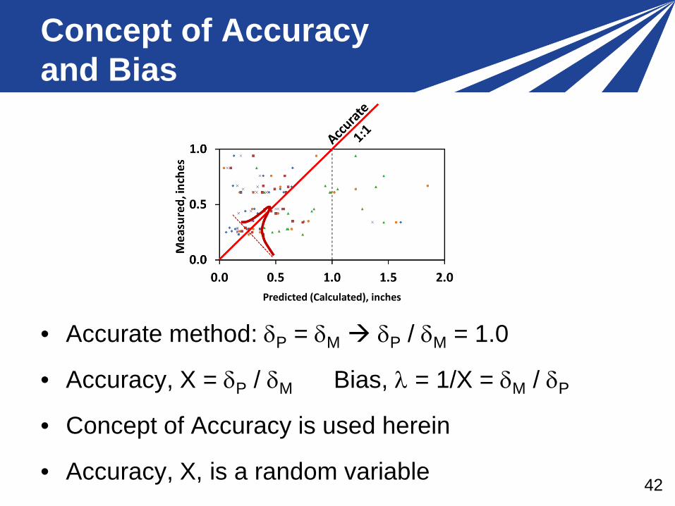
Concept of Accuracy and Bias

• Accurate method: δP = δM δP / δM = 1.0

• Accuracy, X = δP / δM Bias, λ = 1/X = δM / δP

• Concept of Accuracy is used herein

• Accuracy, X, is a random variable

Predicted (Calculated), inches

43

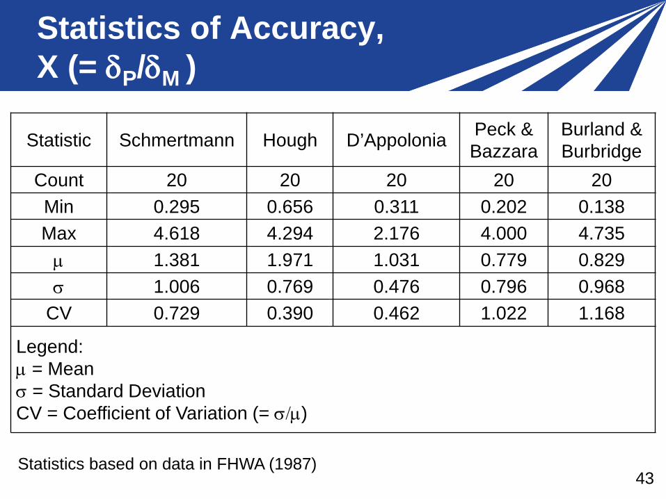
Statistics of Accuracy, X (= δP/δM )

Statistic Schmertmann Hough D’Appolonia Peck & Bazzara

Burland & Burbridge

Count 20 20 20 20 20 Min 0.295 0.656 0.311 0.202 0.138 Max 4.618 4.294 2.176 4.000 4.735

µ 1.381 1.971 1.031 0.779 0.829 σ 1.006 0.769 0.476 0.796 0.968

CV 0.729 0.390 0.462 1.022 1.168

Legend: µ = Mean σ = Standard Deviation CV = Coefficient of Variation (= σ/µ)

Statistics based on data in FHWA (1987)

44

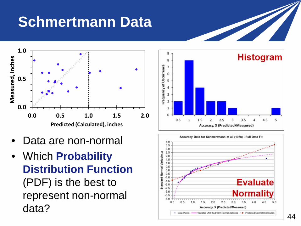
Schmertmann Data

• Data are non-normal • Which Probability

Distribution Function (PDF) is the best to represent non-normal data?

Predicted (Calculated), inches

45

Low

er B

ound

(min

)

Upp

er B

ound

(max

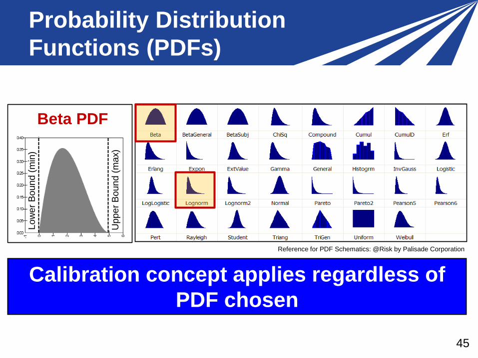
) Beta PDF

Reference for PDF Schematics: @Risk by Palisade Corporation

Probability Distribution Functions (PDFs)

Calibration concept applies regardless of PDF chosen

46

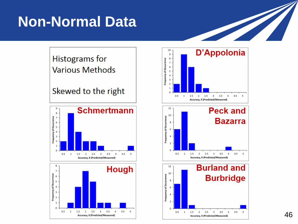
Non-Normal Data

47

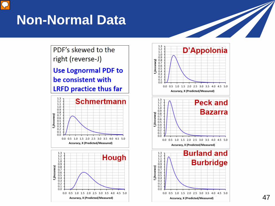
Non-Normal Data

Accuracy, X (Predicted/Measured) Accuracy, X (Predicted/Measured)

Accuracy, X (Predicted/Measured)

Accuracy, X (Predicted/Measured)

Accuracy, X (Predicted/Measured)

48

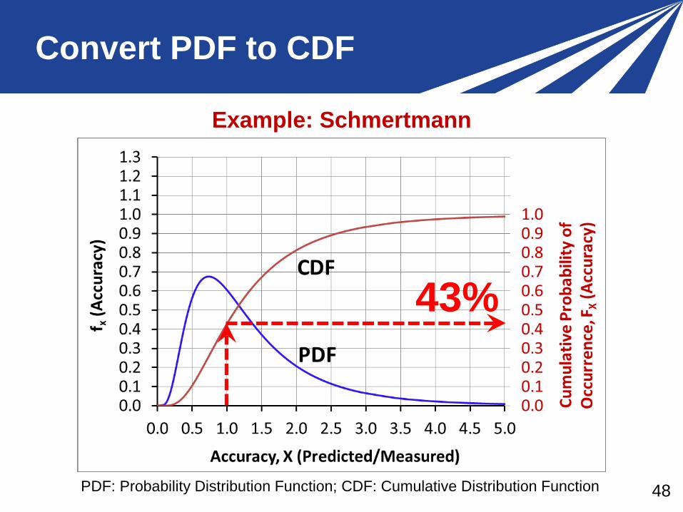
Convert PDF to CDF

Example: Schmertmann

43%

PDF: Probability Distribution Function; CDF: Cumulative Distribution Function

49

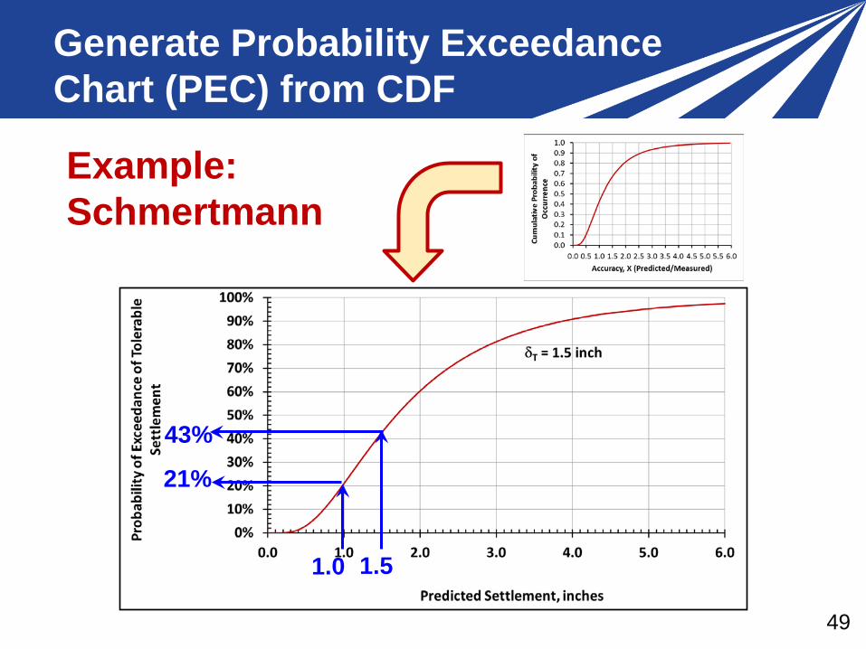
Generate Probability Exceedance Chart (PEC) from CDF

Example: Schmertmann

21%

1.0

43%

1.5

50

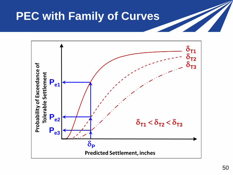
PEC with Family of Curves

δT1 δT2 δT3

δP

Pe3

Pe2

Pe1

δT1 < δT2 < δT3

51

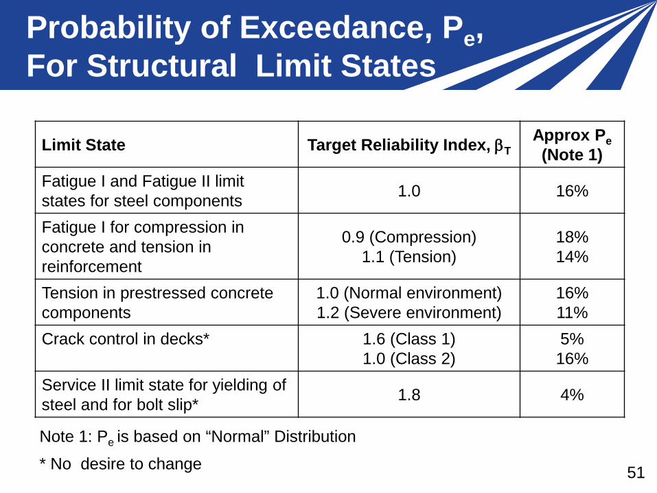
Probability of Exceedance, Pe, For Structural Limit States

Limit State Target Reliability Index, βT Approx Pe (Note 1)

Fatigue I and Fatigue II limit states for steel components 1.0 16%

Fatigue I for compression in concrete and tension in reinforcement

0.9 (Compression) 1.1 (Tension)

18% 14%

Tension in prestressed concrete components

1.0 (Normal environment) 1.2 (Severe environment)

16% 11%

Crack control in decks* 1.6 (Class 1) 1.0 (Class 2)

5% 16%

Service II limit state for yielding of steel and for bolt slip* 1.8 4%

Note 1: Pe is based on “Normal” Distribution

* No desire to change

52

Load Factor γSE

δT1 δT2 δT3

δP

PeT δT Deformation Load Factor γSE = δT/δP

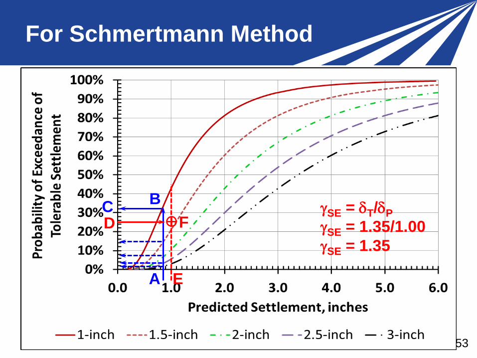
53

For Schmertmann Method

C

E

γSE = δT/δP γSE = 1.35/1.00 γSE = 1.35

A

B

D F

54

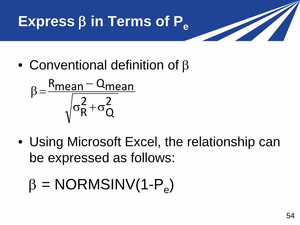
Express β in Terms of Pe

• Conventional definition of β

• Using Microsoft Excel, the relationship can be expressed as follows:

β = NORMSINV(1-Pe)

2Q

2R

meanQmeanR

σ+σ

−=β

55

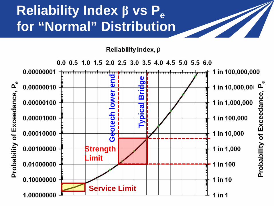
Reliability Index β vs Pe for “Normal” Distribution

Service Limit

Strength Limit

Geo

tech

low

er e

nd

Typi

cal B

ridge

Prob

abili

ty o

f Exc

eeda

nce,

Pe

Prob

abili

ty o

f Exc

eeda

nce,

Pe

56

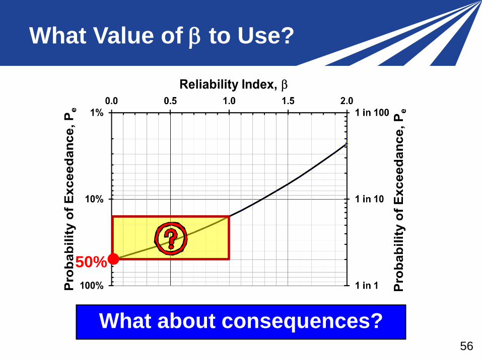
50%

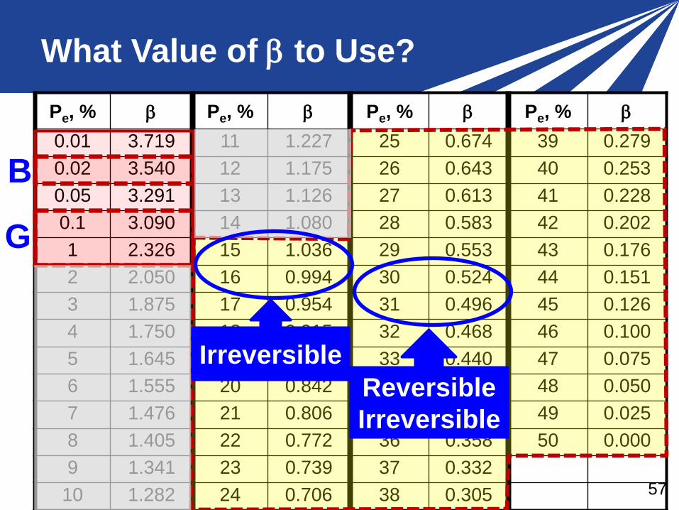
What Value of β to Use?

What about consequences?

57

Pe, % β Pe, % β Pe, % β Pe, % β 0.01 3.719 11 1.227 25 0.674 39 0.279 0.02 3.540 12 1.175 26 0.643 40 0.253 0.05 3.291 13 1.126 27 0.613 41 0.228 0.1 3.090 14 1.080 28 0.583 42 0.202 1 2.326 15 1.036 29 0.553 43 0.176 2 2.050 16 0.994 30 0.524 44 0.151 3 1.875 17 0.954 31 0.496 45 0.126 4 1.750 18 0.915 32 0.468 46 0.100 5 1.645 19 0.878 33 0.440 47 0.075 6 1.555 20 0.842 34 0.412 48 0.050 7 1.476 21 0.806 35 0.385 49 0.025 8 1.405 22 0.772 36 0.358 50 0.000 9 1.341 23 0.739 37 0.332

10 1.282 24 0.706 38 0.305

B

G

Reversible Irreversible

What Value of β to Use?

Irreversible

58

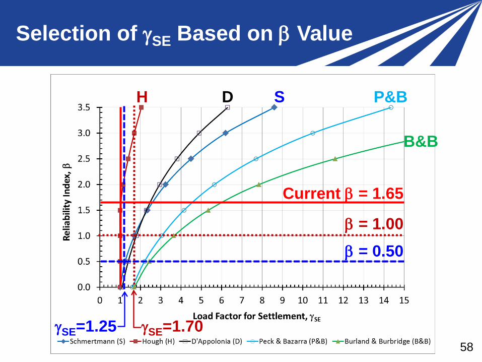
β = 1.00

H D S P&B

B&B

Current β = 1.65

β = 0.50

γSE=1.70 γSE=1.25

Selection of γSE Based on β Value

59

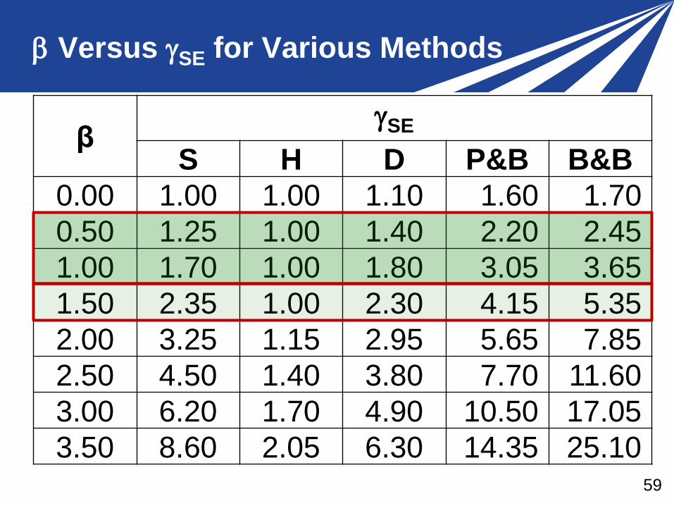
β Versus γSE for Various Methods

β γSE

S H D P&B B&B 0.00 1.00 1.00 1.10 1.60 1.70 0.50 1.25 1.00 1.40 2.20 2.45 1.00 1.70 1.00 1.80 3.05 3.65 1.50 2.35 1.00 2.30 4.15 5.35 2.00 3.25 1.15 2.95 5.65 7.85 2.50 4.50 1.40 3.80 7.70 11.60 3.00 6.20 1.70 4.90 10.50 17.05 3.50 8.60 2.05 6.30 14.35 25.10

60

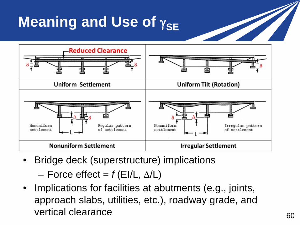
Meaning and Use of γSE

• Bridge deck (superstructure) implications – Force effect = f (EI/L, ∆/L)

• Implications for facilities at abutments (e.g., joints, approach slabs, utilities, etc.), roadway grade, and vertical clearance

61

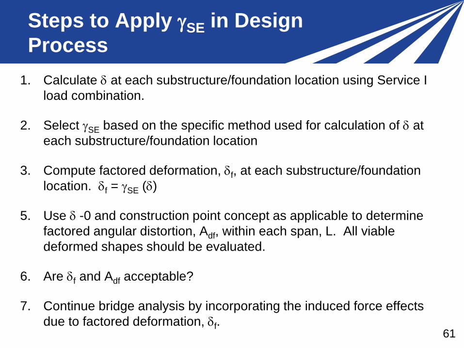
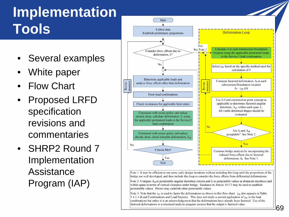
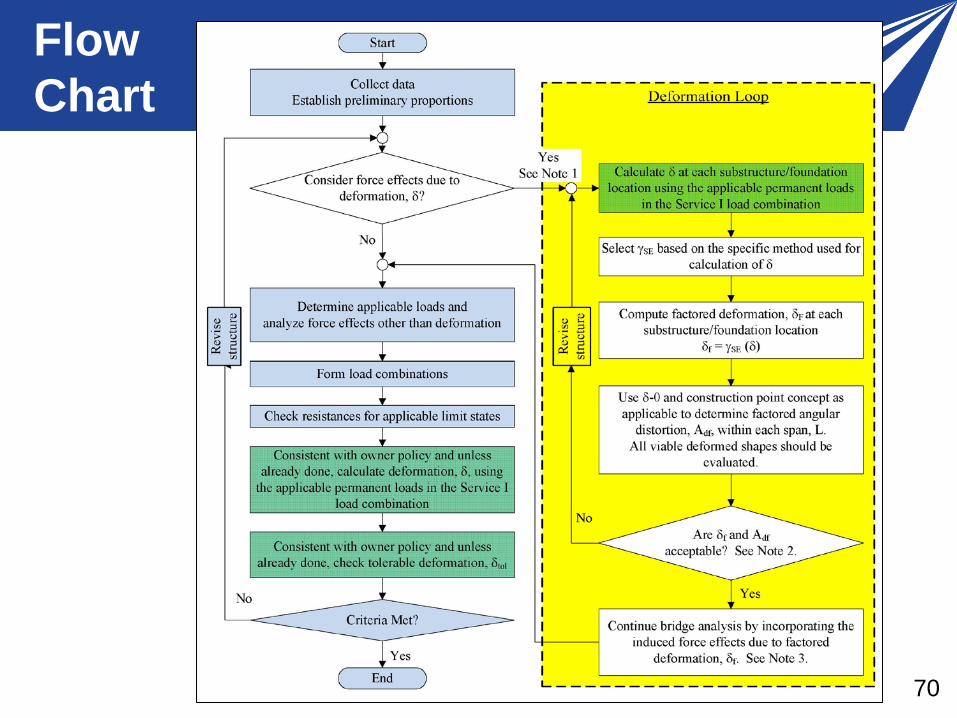
Steps to Apply γSE in Design Process

1. Calculate δ at each substructure/foundation location using Service I load combination.

2. Select γSE based on the specific method used for calculation of δ at each substructure/foundation location

3. Compute factored deformation, δf, at each substructure/foundation location. δf = γSE (δ)

5. Use δ -0 and construction point concept as applicable to determine factored angular distortion, Adf, within each span, L. All viable deformed shapes should be evaluated.

6. Are δf and Adf acceptable?

7. Continue bridge analysis by incorporating the induced force effects due to factored deformation, δf.

62

Induced Force Effects Due to γSE

• Deformations generate additional force effects (moments) – Load factor of SE is similar to PS, CR, SH, TU, and TG

• The value of γSE must not be taken literally – γSE = 1.25 does not mean that the total force effects

will increase by 25% – γSE is only one component in a load combination

• The additional moments due to effect of deformations are very dependent on the stiffness of the bridge (EI/L) as well as the angular distortion (∆/L)

63

Results of Limited Parametric Study

• Several 2- and 3-span steel and pre-stressed concrete continuous bridges from NCHRP Project 12-78. – Considered full angular distortion (Moulton’s criteria)

• Finding: An increase in factored Strength I moments on the order of as little as 10% for the more flexible units to more than double the moment from only factored dead and live load moments for the stiffer units. – Finding is based on elastic analysis and without

consideration of creep, which could significantly reduce the moments, especially for relatively stiff concrete bridges.

– Additional examples will be developed.

64

Effect of Foundation Deformations On Superstructures

• For all bridges, stiffness should be appropriate to considered limit state.

• The effect of continuity with the substructure should be considered.

• Consider all viable deformation shapes.

• For concrete bridges, the determination of the stiffness of the bridge components should consider the effect of cracking, creep, and other inelastic responses.

65

Proposed Modifications To AASHTO

• Article 10.5.2 – “Service Limit States”

• Article 10.5.2 is cross-referenced in articles for various foundations types such as spread footings, driven piles, drilled shafts, micropiles, retaining walls, joints, etc.

• Making change in Article 10.5.2 will permeate through all the relevant sections of AASHTO.

66

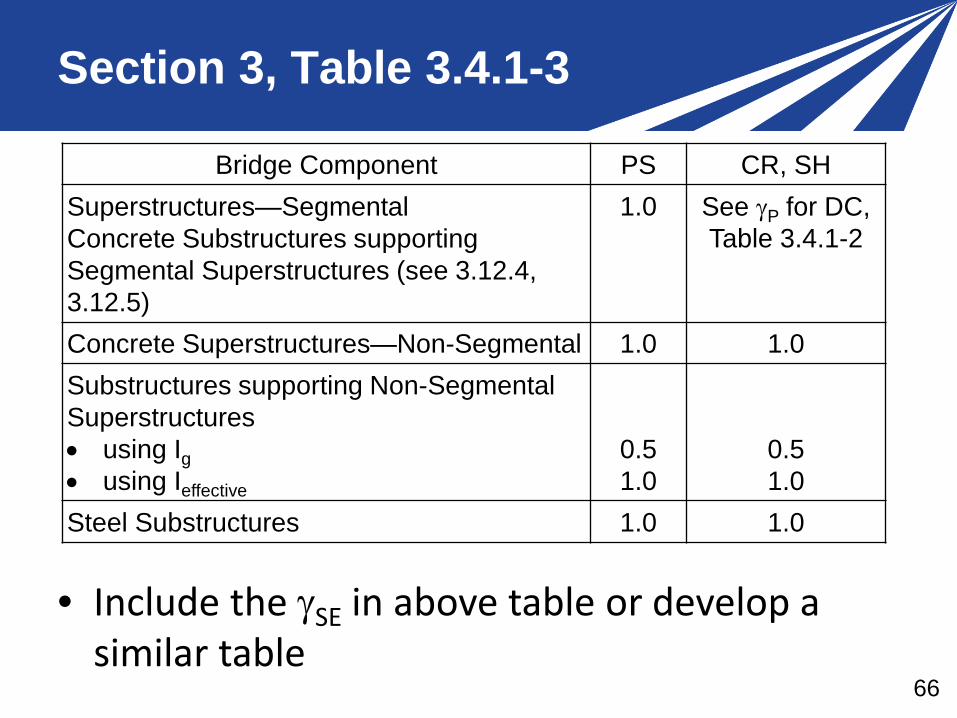
Section 3, Table 3.4.1-3

Bridge Component PS CR, SH Superstructures—Segmental Concrete Substructures supporting Segmental Superstructures (see 3.12.4, 3.12.5)

1.0 See γP for DC, Table 3.4.1-2

Concrete Superstructures—Non-Segmental 1.0 1.0 Substructures supporting Non-Segmental Superstructures • using Ig • using Ieffective

0.5 1.0

0.5 1.0

Steel Substructures 1.0 1.0

• Include the γSE in above table or develop a similar table

67

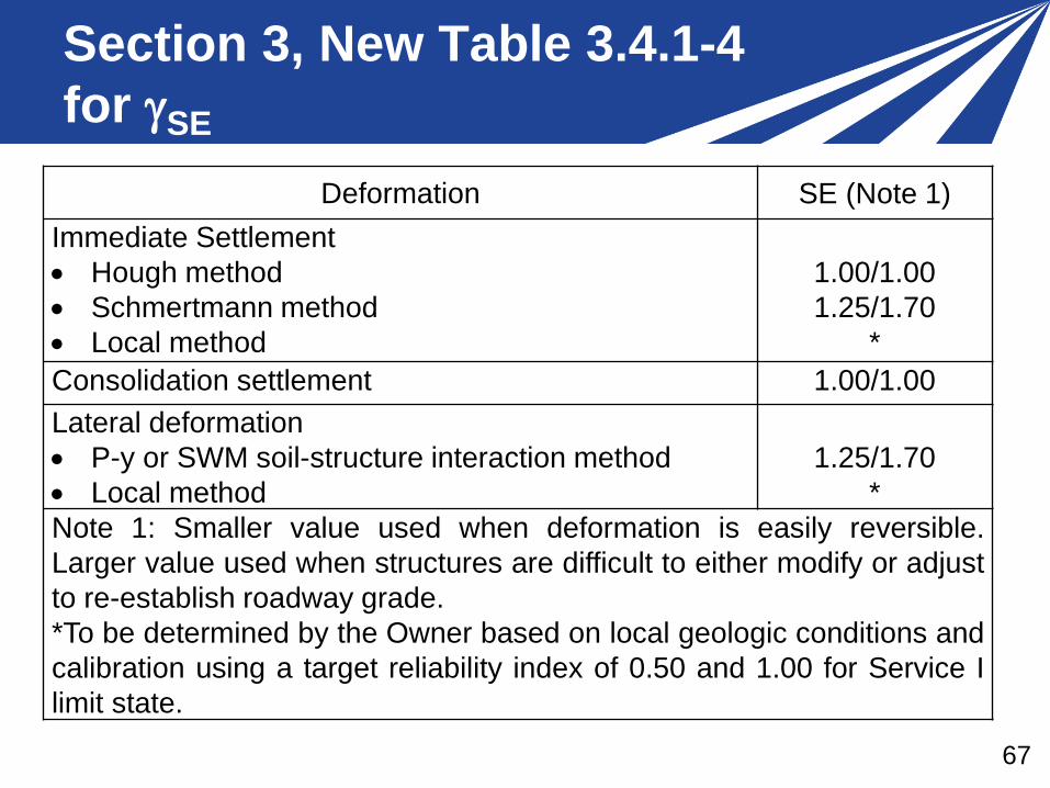
Section 3, New Table 3.4.1-4 for γSE

Deformation SE (Note 1) Immediate Settlement • Hough method • Schmertmann method • Local method

1.00/1.00 1.25/1.70

* Consolidation settlement 1.00/1.00 Lateral deformation • P-y or SWM soil-structure interaction method • Local method

1.25/1.70

* Note 1: Smaller value used when deformation is easily reversible. Larger value used when structures are difficult to either modify or adjust to re-establish roadway grade. *To be determined by the Owner based on local geologic conditions and calibration using a target reliability index of 0.50 and 1.00 for Service I limit state.

68

For Consideration by T-5/T-15

• Modification to Sections 3 and 10 to implement recommendations ready for: – Deformation Load factors, γSE

– δ – 0 concept with construction point and estimation of relevant deformation values

– Schmertmann method – Commentaries – Updated references

69

Implementation Tools

• Several examples • White paper • Flow Chart • Proposed LRFD

specification revisions and commentaries

• SHRP2 Round 7 Implementation Assistance Program (IAP)

70

Flow Chart

71

Closing Comments

• Consideration of foundation deformations in bridge design is not new.

• The uncertainty in predicted deformations can now be quantified through the mechanism of SE load factor, γSE.

• The calibration process is general and can be applied to any foundation or wall type and any type of deformation.

• Microsoft Excel®-based calibration processes have been developed.

• Framework for inclusion of future calibrations is provided through proposed Table 3.4.1-4 for γSE.

72

Closing Comments

• Tools for implementation are available.

– SHRP2 Round 7 Implementation Assistance Program (IAP)

• Application period, April 1 – 29, 2016

• Informational webinars, February – March 2016

– Training seminars, TBD

73

Questions and Contacts

• FHWA: Matthew DeMarco, SHRP2 Renewal Program Engineer – Structures, matthew.demarco@dot.gov

• AASHTO: Patricia Bush, Program Manager for Engineering, pbush@aashto.org

Pam Hutton, AASHTO SHRP2 Implementation Manager, phutton@aashto.org

• NCS GeoResources, LLC: Naresh C. Samtani, PhD, PE, naresh@ncsgeoresources.com

• Modjeski and Masters, Inc.: John M. Kulicki, PhD, PE, JMKulicki@modjeski.com

http://SHRP2.transportation.org or https://www.fhwa.dot.gov/goshrp2