Embed Size (px)
Citation preview

Service Management – Capacity Planning and Queuing Models Univ.-Prof. Dr.-Ing. Wolfgang Maass Chair in Economics – Information and Service Systems (ISS) Saarland University, Saarbrücken, Germany WS 2011/2012 Thursdays, 8:00 – 10:00 a.m. Room HS 024, B4 1
Univ.-Prof. Dr.-Ing. Wolfgang Maass
19.01.12 Slide 2
General Agenda
1. Introduction 2. Service Strategy 3. New Service Development (NSD) 4. Service Quality 5. Supporting Facility 6. Forecasting Demand for Services 7. Managing Demand 8. Managing Capacity 9. Managing Queues 10. Capacity Planning and Queuing Models 11. Services and Information Systems 12. ITIL Service Design 13. IT Service Infrastructures 14. Summary and Outlook
Univ.-Prof. Dr.-Ing. Wolfgang Maass
19.01.12 Slide 3
Agenda Lecture 10
• Different Views of Managing Queues • 3) Economic View
• Capacity Planning • Queuing Models
• Classification of Queuing Models • Overview of Queuing Models • Standard M/M/1 Model (1) • Features of Queuing Systems (Repetition) • Standard M/M/1 Model (2)
Univ.-Prof. Dr.-Ing. Wolfgang Maass
19.01.12 Slide 4
Different Views of Managing Queues
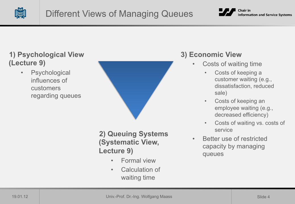
3) Economic View • Costs of waiting time
• Costs of keeping a customer waiting (e.g., dissatisfaction, reduced sale)
• Costs of keeping an employee waiting (e.g., decreased efficiency)
• Costs of waiting vs. costs of service
• Better use of restricted capacity by managing queues
1) Psychological View (Lecture 9)
• Psychological influences of customers regarding queues
2) Queuing Systems (Systematic View, Lecture 9)
• Formal view • Calculation of
waiting time
Univ.-Prof. Dr.-Ing. Wolfgang Maass
19.01.12 Slide 5
3) Economic View: Capacity Planning
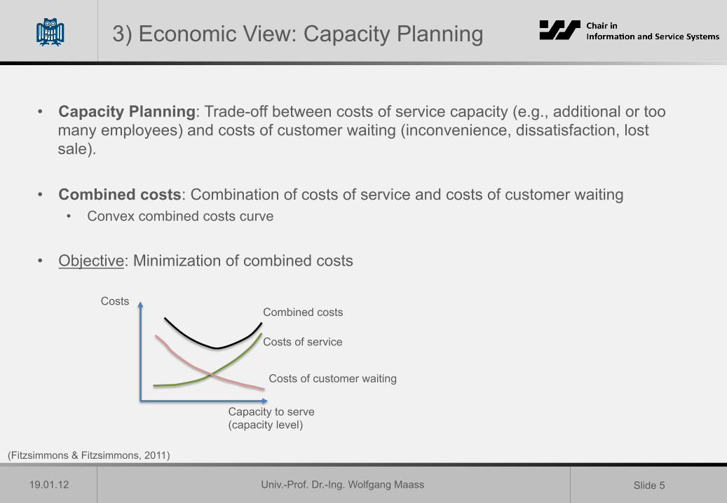
• Capacity Planning: Trade-off between costs of service capacity (e.g., additional or too many employees) and costs of customer waiting (inconvenience, dissatisfaction, lost sale).
• Combined costs: Combination of costs of service and costs of customer waiting • Convex combined costs curve
• Objective: Minimization of combined costs
Costs
Capacity to serve (capacity level)
Combined costs
Costs of service
Costs of customer waiting
(Fitzsimmons & Fitzsimmons, 2011)
Univ.-Prof. Dr.-Ing. Wolfgang Maass
19.01.12 Slide 6
Agenda Lecture 10
• Different Views of Managing Queues • 3) Economic View
• Capacity Planning • Queuing Models
• Classification of Queuing Models • Overview of Queuing Models • Standard M/M/1 Model (1) • Features of Queuing Systems (Repetition) • Standard M/M/1 Model (2)

Univ.-Prof. Dr.-Ing. Wolfgang Maass
19.01.12 Slide 7
3) Economic View: Capacity Planning
Minimizing the sum of costs of service and customer waiting costs (combined costs) • If customers and employees belong to the same organization (e.g., secretarial pool):
Waiting and service costs are equally important • Cost of waiting time is average salary of employees (employees are internal customers) • Relationship between costs:
• Service capacity is increased by employing further staff • This rises the service costs • However: Costs of waiting are decreased
• Adding costs of service and waiting: Combined costs
• Objective: Minimization of combined costs: • Identification of service capacity level with lowest combined costs (= optimum)
(Fitzsimmons & Fitzsimmons, 2011)
Univ.-Prof. Dr.-Ing. Wolfgang Maass
19.01.12 Slide 8
3) Economic View: Capacity Planning
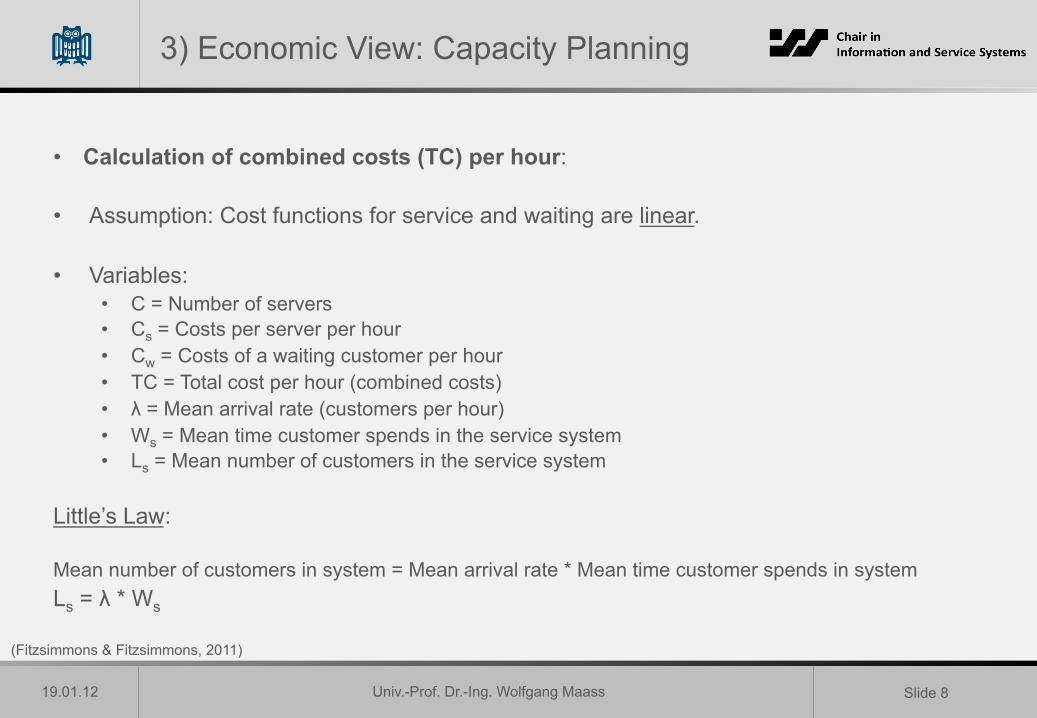
• Calculation of combined costs (TC) per hour:
• Assumption: Cost functions for service and waiting are linear.
• Variables: • C = Number of servers • Cs = Costs per server per hour • Cw = Costs of a waiting customer per hour • TC = Total cost per hour (combined costs) • λ = Mean arrival rate (customers per hour) • Ws = Mean time customer spends in the service system • Ls = Mean number of customers in the service system
Little’s Law: Mean number of customers in system = Mean arrival rate * Mean time customer spends in system Ls = λ * Ws
(Fitzsimmons & Fitzsimmons, 2011)

Univ.-Prof. Dr.-Ing. Wolfgang Maass
19.01.12 Slide 9
3) Economic View: Capacity Planning
• Total costs per hour = Total costs of service per hour + Total waiting costs per hour • Total costs per hour = Costs per server per hour * Number of servers + Costs of a waiting
customer per hour * Mean arrival rate * Mean time customer spends in the service system
• TC = Cs * C + Cw * λ * Ws
• <=> TC = Cs * C + Cw * Ls According to Little’s Law Ls and Ws: Calculated in the next section (queuing models). Assumption of linear cost functions:
Not realistic if customers and employees belong to different organizations (e.g., costs of customer waiting increase strongly if there are long queues: Dissatisfaction, telling friends about bad service (negative word-of-mouth)). However: Linear cost functions are easier to calculate.
(Fitzsimmons & Fitzsimmons, 2011)
Univ.-Prof. Dr.-Ing. Wolfgang Maass
19.01.12 Slide 10
3) Economic View: Capacity Planning
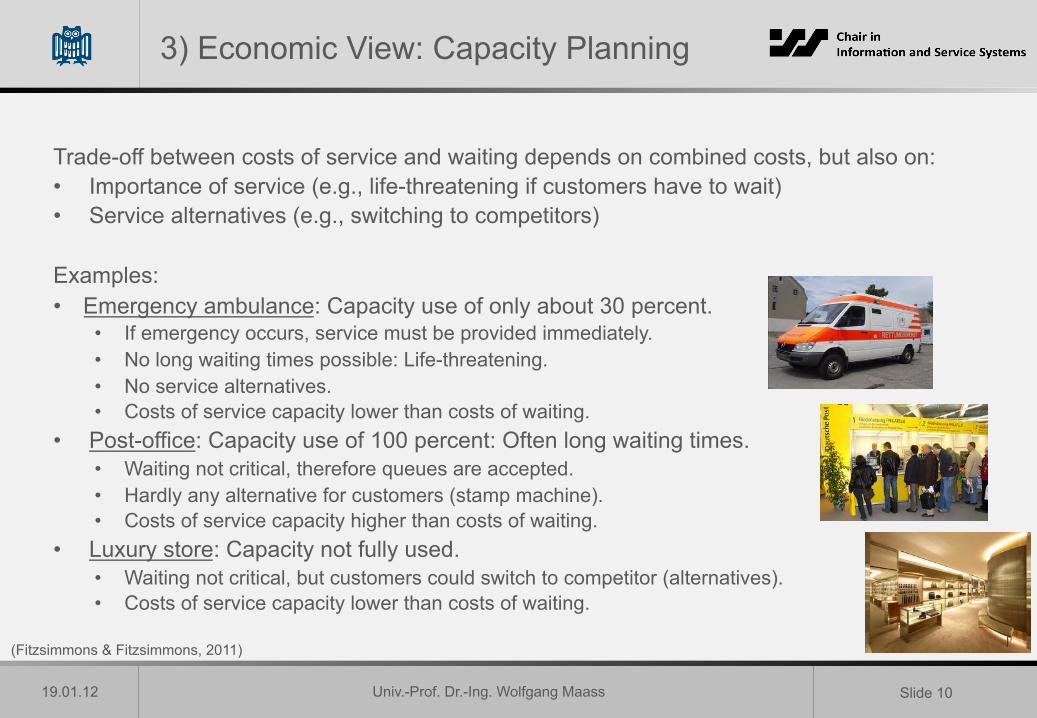
Trade-off between costs of service and waiting depends on combined costs, but also on: • Importance of service (e.g., life-threatening if customers have to wait) • Service alternatives (e.g., switching to competitors)
Examples: • Emergency ambulance: Capacity use of only about 30 percent.
• If emergency occurs, service must be provided immediately. • No long waiting times possible: Life-threatening. • No service alternatives. • Costs of service capacity lower than costs of waiting.
• Post-office: Capacity use of 100 percent: Often long waiting times. • Waiting not critical, therefore queues are accepted. • Hardly any alternative for customers (stamp machine). • Costs of service capacity higher than costs of waiting.
• Luxury store: Capacity not fully used. • Waiting not critical, but customers could switch to competitor (alternatives). • Costs of service capacity lower than costs of waiting.
(Fitzsimmons & Fitzsimmons, 2011)

Univ.-Prof. Dr.-Ing. Wolfgang Maass
19.01.12 Slide 11
Brainteaser
• Regarding capacity planning, a trade-off has to be made between two factors. Describe which factors are meant and why there is a trade-off.
• Please choose two influencing variables of the trade-off decision and give an example where these could occur in practice.
10 Minutes
Univ.-Prof. Dr.-Ing. Wolfgang Maass
19.01.12 Slide 12
Agenda Lecture 10
• Different Views of Managing Queues • 3) Economic View
• Capacity Planning • Queuing Models
• Classification of Queuing Models • Overview of Queuing Models • Standard M/M/1 Model (1) • Features of Queuing Systems (Repetition) • Standard M/M/1 Model (2)

Univ.-Prof. Dr.-Ing. Wolfgang Maass
19.01.12 Slide 13
3) Economic View: Queuing Models: Classification of Queuing Models
• Queuing Models: Analytical models for analyzing queues of waiting customers.
• Mean time customer spends in the service system (Ws) and mean number of customers in the service system (Ls) necessary for capacity planning:
• Can be calculated using queuing models
• Classification of queuing models:
• Classification of queuing models with single or parallel servers (several employees serving several customers at the same time, e.g., 3 cashiers in a supermarket).
• Notation: A/B/C (defines to which class a model belongs). • A = Distribution of time between arrivals of customers • B = Distribution of service times • C = Number of parallel servers (e.g., several cashiers)
Examples of notation: • A: M = Poisson distributed arrivals • B: M = Exponential service times distribution, G = General service times distribution • C: 1 = One single server, c = Several servers, ∞ = Self-service
(Fitzsimmons & Fitzsimmons, 2011)

Univ.-Prof. Dr.-Ing. Wolfgang Maass
19.01.12 Slide 14
3) Economic View: Queuing Models: Classification of Queuing Models
State of queuing models: • Transient: Values of model depend on time (e.g., weeks before Christmas versus standard
days in shops) • Steady: Values are independent of time
• Values vary at beginning of operations (e.g., opening days of a new shop with long queues) • After some time: Steady state is reached (statistical equilibrium): Long-term capacity planning
• Distribution of arrival: • Poisson
• Length of queue: • Standard (infinite): No restrictions for length • Finite: Length is limited (e.g., due to little space on a parking lot)
• Service time distribution: • Exponential • General: Any standard distribution of service times with mean and variance
• Number of servers: • Single (one server) • Multiple (several servers) • Self-service (no servers)
(Fitzsimmons & Fitzsimmons, 2011)
Univ.-Prof. Dr.-Ing. Wolfgang Maass
19.01.12 Slide 15
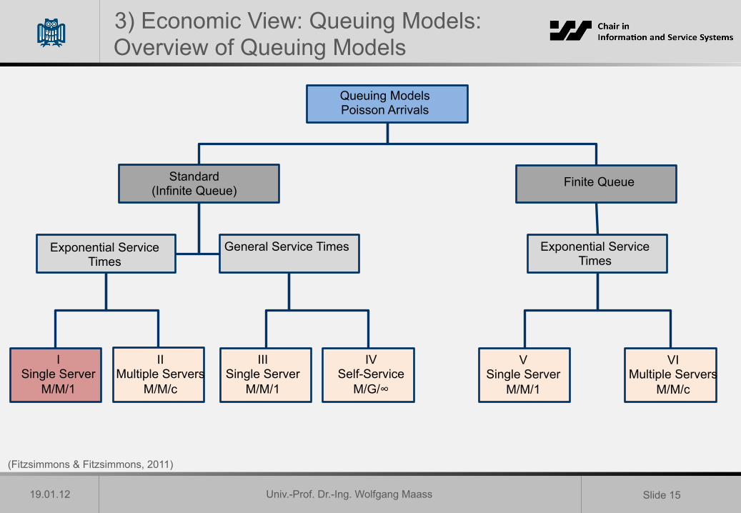
3) Economic View: Queuing Models: Overview of Queuing Models
Queuing Models Poisson Arrivals
Standard (Infinite Queue)
Finite Queue
V Single Server
M/M/1
Exponential Service Times
General Service Times Exponential Service Times
(Fitzsimmons & Fitzsimmons, 2011)
VI Multiple Servers
M/M/c
IV Self-Service
M/G/∞
III Single Server
M/M/1
II Multiple Servers
M/M/c
I Single Server
M/M/1
Univ.-Prof. Dr.-Ing. Wolfgang Maass
19.01.12 Slide 16
Agenda Lecture 10
• Different Views of Managing Queues • 3) Economic View
• Capacity Planning • Queuing Models
• Classification of Queuing Models • Overview of Queuing Models • Standard M/M/1 Model (1) • Features of Queuing Systems (Repetition) • Standard M/M/1 Model (2)

Univ.-Prof. Dr.-Ing. Wolfgang Maass
19.01.12 Slide 17
3) Economic View: Queuing Models: Standard M/M/1 Model (1)
Standard M/M/1 Model: • M = Poisson distribution of arrival rate • M = Exponential service time distribution • 1 = One server providing a service to the customers (single server)
M/M/1 = Single-server model with Poisson distributed arrival rate and exponential service time distribution Schematic for the model:
Customers queuing in the service system
One server serving one customer after the other
Customer being served
(Fitzsimmons & Fitzsimmons, 2011)
Single server
Univ.-Prof. Dr.-Ing. Wolfgang Maass
19.01.12 Slide 18
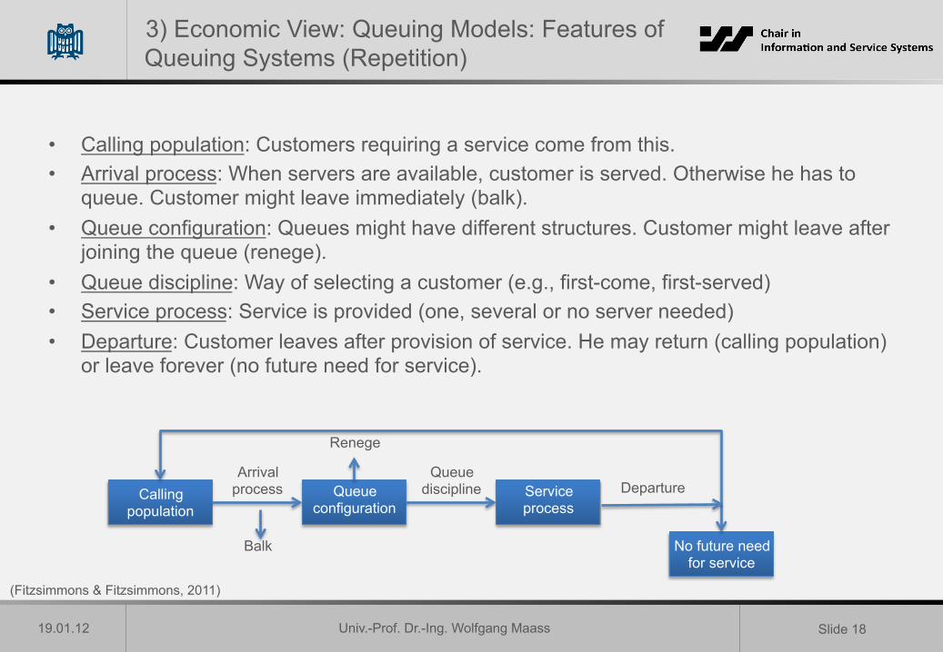
3) Economic View: Queuing Models: Features of Queuing Systems (Repetition)
• Calling population: Customers requiring a service come from this. • Arrival process: When servers are available, customer is served. Otherwise he has to
queue. Customer might leave immediately (balk). • Queue configuration: Queues might have different structures. Customer might leave after
joining the queue (renege). • Queue discipline: Way of selecting a customer (e.g., first-come, first-served) • Service process: Service is provided (one, several or no server needed) • Departure: Customer leaves after provision of service. He may return (calling population)
or leave forever (no future need for service).
Calling population
Queue configuration
Service process
No future need for service
Balk
Renege
Queue discipline Departure
Arrival process
(Fitzsimmons & Fitzsimmons, 2011)

Univ.-Prof. Dr.-Ing. Wolfgang Maass
19.01.12 Slide 19
Agenda Lecture 10
• Different Views of Managing Queues • 3) Economic View
• Capacity Planning • Queuing Models
• Classification of Queuing Models • Overview of Queuing Models • Standard M/M/1 Model (1) • Features of Queuing Systems (Repetition) • Standard M/M/1 Model (2)
Univ.-Prof. Dr.-Ing. Wolfgang Maass
19.01.12 Slide 20
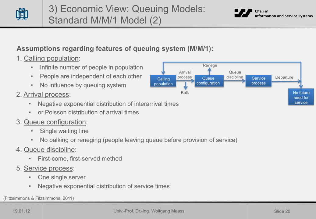
3) Economic View: Queuing Models: Standard M/M/1 Model (2)
Assumptions regarding features of queuing system (M/M/1): 1. Calling population:
• Infinite number of people in population • People are independent of each other • No influence by queuing system
2. Arrival process: • Negative exponential distribution of interarrival times • or Poisson distribution of arrival times
3. Queue configuration: • Single waiting line • No balking or reneging (people leaving queue before provision of service)
4. Queue discipline: • First-come, first-served method
5. Service process: • One single server • Negative exponential distribution of service times
Calling population
Queue configuration
Service process
No future need for service
Balk
Renege
Queue discipline Departure
Arrival process
(Fitzsimmons & Fitzsimmons, 2011)
Univ.-Prof. Dr.-Ing. Wolfgang Maass
19.01.12 Slide 21
3) Economic View: Queuing Models: Standard M/M/1 Model (2)
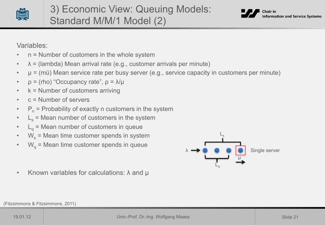
Variables: • n = Number of customers in the whole system • λ = (lambda) Mean arrival rate (e.g., customer arrivals per minute) • µ = (mü) Mean service rate per busy server (e.g., service capacity in customers per minute) • ρ = (rho) “Occupancy rate”, ρ = λ/µ • k = Number of customers arriving • c = Number of servers • Pn = Probability of exactly n customers in the system • Ls = Mean number of customers in the system • Lq = Mean number of customers in queue • Ws = Mean time customer spends in system • Wq = Mean time customer spends in queue
• Known variables for calculations: λ and µ
Lq
Ls
λ µ
Single server
(Fitzsimmons & Fitzsimmons, 2011)
Univ.-Prof. Dr.-Ing. Wolfgang Maass
19.01.12 Slide 22
3) Economic View: Queuing Models: Standard M/M/1 Model (2)
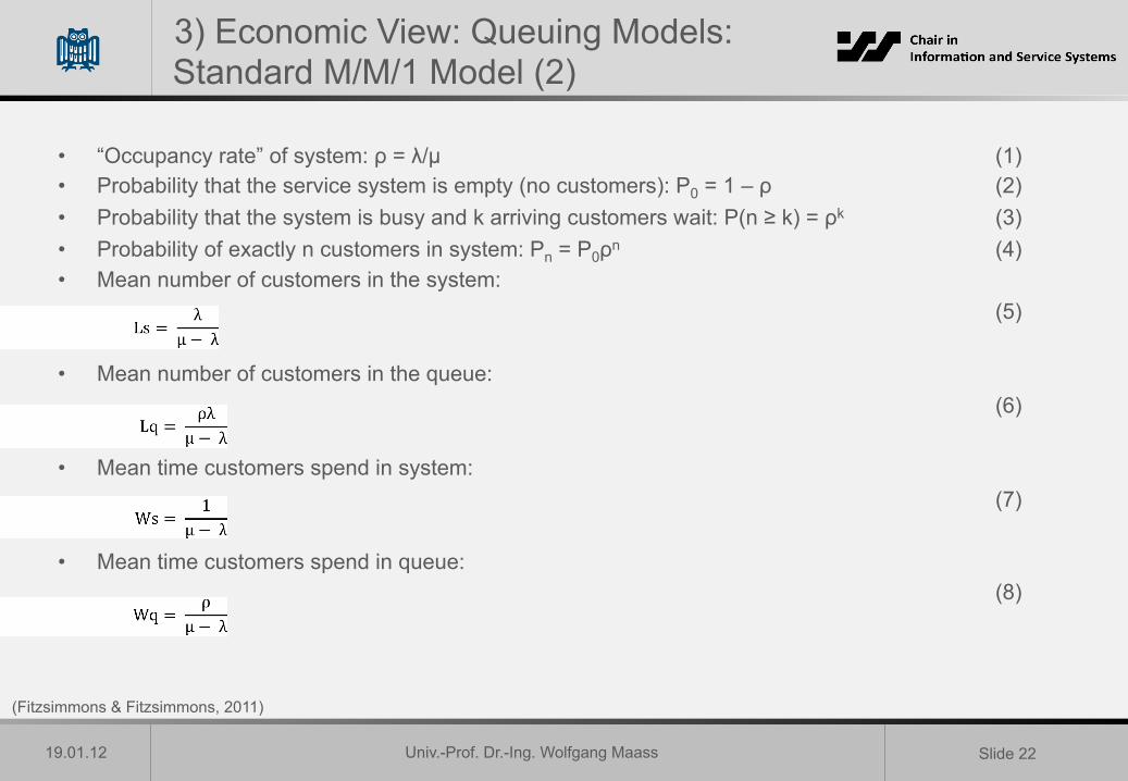
• “Occupancy rate” of system: ρ = λ/µ (1) • Probability that the service system is empty (no customers): P0 = 1 – ρ (2) • Probability that the system is busy and k arriving customers wait: P(n ≥ k) = ρk (3) • Probability of exactly n customers in system: Pn = P0ρn (4) • Mean number of customers in the system:
(5) • Mean number of customers in the queue:
(6) • Mean time customers spend in system:
(7) • Mean time customers spend in queue:
(8)
(Fitzsimmons & Fitzsimmons, 2011)
Univ.-Prof. Dr.-Ing. Wolfgang Maass
19.01.12 Slide 23
3) Economic View: Queuing Models: Standard M/M/1 Model (2)
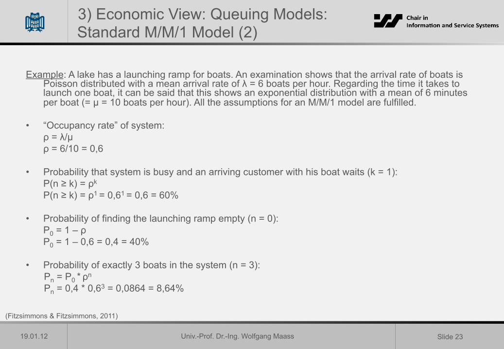
Example: A lake has a launching ramp for boats. An examination shows that the arrival rate of boats is Poisson distributed with a mean arrival rate of λ = 6 boats per hour. Regarding the time it takes to launch one boat, it can be said that this shows an exponential distribution with a mean of 6 minutes per boat (= µ = 10 boats per hour). All the assumptions for an M/M/1 model are fulfilled.
• “Occupancy rate” of system:
ρ = λ/µ ρ = 6/10 = 0,6 • Probability that system is busy and an arriving customer with his boat waits (k = 1):
P(n ≥ k) = ρk
P(n ≥ k) = ρ1 = 0,61 = 0,6 = 60% • Probability of finding the launching ramp empty (n = 0):
P0 = 1 – ρ P0 = 1 – 0,6 = 0,4 = 40%
• Probability of exactly 3 boats in the system (n = 3):
Pn = P0 * ρn
Pn = 0,4 * 0,63 = 0,0864 = 8,64%
(Fitzsimmons & Fitzsimmons, 2011)
Univ.-Prof. Dr.-Ing. Wolfgang Maass
19.01.12 Slide 24
3) Economic View: Queuing Models: Standard M/M/1 Model (2)
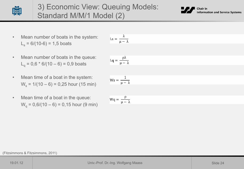
• Mean number of boats in the system: Ls = 6/(10-6) = 1,5 boats
• Mean number of boats in the queue:
Lq = 0,6 * 6/(10 – 6) = 0,9 boats • Mean time of a boat in the system:
Ws = 1/(10 – 6) = 0,25 hour (15 min) • Mean time of a boat in the queue:
Wq = 0,6/(10 – 6) = 0,15 hour (9 min)
(Fitzsimmons & Fitzsimmons, 2011)
Univ.-Prof. Dr.-Ing. Wolfgang Maass
19.01.12 Slide 25
3) Economic View: Queuing Models: Standard M/M/1 Model (2)
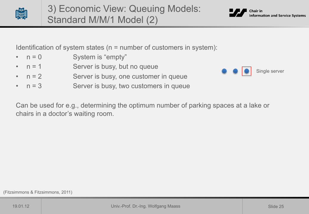
Identification of system states (n = number of customers in system): • n = 0 System is “empty” • n = 1 Server is busy, but no queue • n = 2 Server is busy, one customer in queue • n = 3 Server is busy, two customers in queue
Can be used for e.g., determining the optimum number of parking spaces at a lake or chairs in a doctor’s waiting room.
Single server
(Fitzsimmons & Fitzsimmons, 2011)
Univ.-Prof. Dr.-Ing. Wolfgang Maass
19.01.12 Slide 26
Outlook
1. Introduction 2. Service Strategy 3. New Service Development (NSD) 4. Service Quality 5. Supporting Facility 6. Forecasting Demand for Services 7. Managing Demand 8. Managing Capacity 9. Managing Queues 10. Capacity Planning and Queuing Models 11. Services and Information Systems 12. ITIL Service Design 13. IT Service Infrastructures 14. Summary and Outlook
Univ.-Prof. Dr.-Ing. Wolfgang Maass
19.01.12 Slide 27
Literature
Books: • Fitzsimmons, J. A. & Fitzsimmons, M. J. (2011), Service Management - Operations, Strategy, Information Technology,
McGraw – Hill.

Univ.-Prof. Dr.-Ing. Wolfgang Maass
Univ.-Prof. Dr.-Ing. Wolfgang Maass Chair in Information and Service Systems Saarland University, Germany