Session 1b Applications, genome sequencing, RNA …cassavabase.wikispaces.com/file/view/Session1bSeqApplications_LQ...2003 Drosophila genome 250k Sanger ESTs 700 175 2005 ... With

Session 1b Applications, genome sequencing, RNA Seq, GBS

Applications: RNASeq and GBS (Simon)Making RNA-Seq libraries

Making GBS librariesQuality filtering Next-gen sequence data

Applications for RNA-Seq data: finding differentially-expressed genes.Applications for GBS: genetic map making, Genomic Selection (basic intrduction)

1Sunday, April 14, 13

Introduction to gene expression studies

• Why it is so useful

• What you can learn with it.


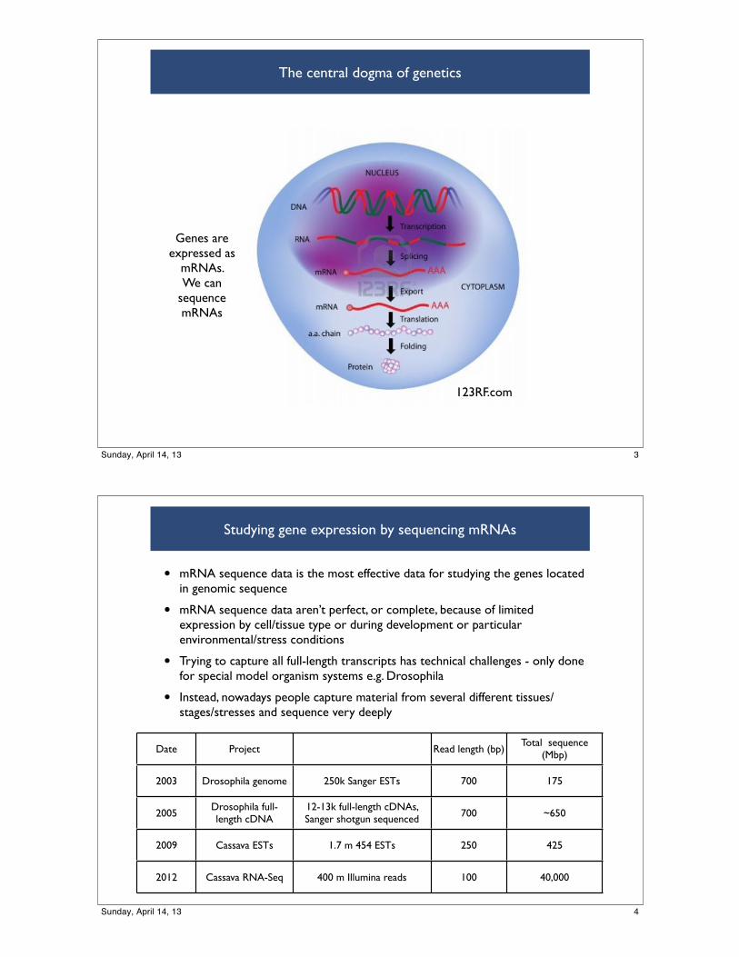
The central dogma of genetics

123RF.com

Genes are expressed as

mRNAs. We can

sequence mRNAs


Studying gene expression by sequencing mRNAs

• mRNA sequence data is the most effective data for studying the genes located in genomic sequence

• mRNA sequence data aren’t perfect, or complete, because of limited expression by cell/tissue type or during development or particular environmental/stress conditions

• Trying to capture all full-length transcripts has technical challenges - only done for special model organism systems e.g. Drosophila

• Instead, nowadays people capture material from several different tissues/stages/stresses and sequence very deeply

Date Project Read length (bp)Total sequence

(Mbp)

2003 Drosophila genome 250k Sanger ESTs 700 175

2005Drosophila full-length cDNA

12-13k full-length cDNAs, Sanger shotgun sequenced 700 ~650

2009 Cassava ESTs 1.7 m 454 ESTs 250 425

2012 Cassava RNA-Seq 400 m Illumina reads 100 40,000


DNA and genome sequencing


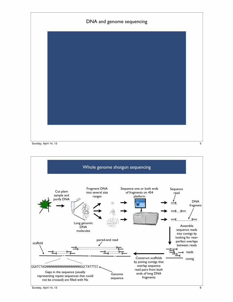
Cut plant sample and purify DNA

Fragment DNA into several size

ranges

Assemble sequence reads into contigs by

looking for near-perfect overlaps between reads

contig

reads

Long genomic DNA

molecules

Sequence one or both ends of fragments on 454

platform

Construct scaffolds by joining contigs that

overlap sequence read pairs from both ends of long DNA

fragments

GGATCTAGNNNNNNNNNNNNNNNNNNNGGCTATTTCCGaps in the sequence (usually

representing repeat sequences that could not be crossed) are filled with Ns

Genome sequence

Sequence read

DNA fragment

paired-end readscaffold

Whole genome shotgun sequencing


The genome of cassava has been sequenced

• JGI CSP pilot 1x coverage from over 700,000 Sanger shotgun reads using plasmid and fosmid libraries

• Main sequencing effort: partnership with 454 Life Sciences (Roche), Steve Rounsley, Dan Rokhsar, Chinnappa Kodira, and Tim Harkins

• 454 GS FLX Titanium platform. Nearly 61 million 454 reads (single and paired-end) were generated and combined with the Sanger data from the pilot project as input for genome assembly

• $1.3 million grant by the Bill & Melinda Gates Foundation


Cassava assembly v1

• 11,243 scaffolds

• 416Mb (26% N = gaps)

• scaffold N50/L50 514/180kb

• cucumber assemblies N50/L50 ~60 / ~900kb (Therese’s presentation)

• Cassava has an estimated genome size of ~760Mb

• Remaining 300Mb estimated to be non-genic, repetitive

• 1) A large fraction of reads (both Sanger and 454) were not used by the assembly software, and were primarily repetitive in nature.

• 2) 95% of publicly-available cassava ESTs map to the assembly.


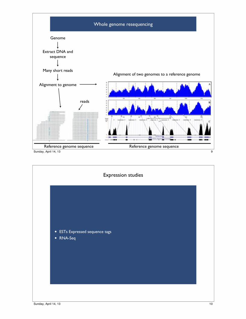
Whole genome resequencing

Genome

Many short reads

Alignment to genome

Alignment of two genomes to a reference genome

Extract DNA and sequence

Reference genome sequenceReference genome sequence

reads


Expression studies

• ESTs Expressed sequence tags

• RNA-Seq


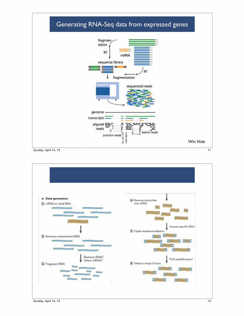
Generating RNA-Seq data from expressed genes

RNA-seq

49

Generate Library(Martin, Wang, 2011)

50

Win Hide


RNA-seq

49

Generate Library(Martin, Wang, 2011)

50

Ligate and size select

51

Data analysisLow quality reads X

Sequence errors X

52


Ligate and size select

51

Data analysisLow quality reads X

Sequence errors X

52

Assemblycorrect assembly errors

53

Estimate expression

54


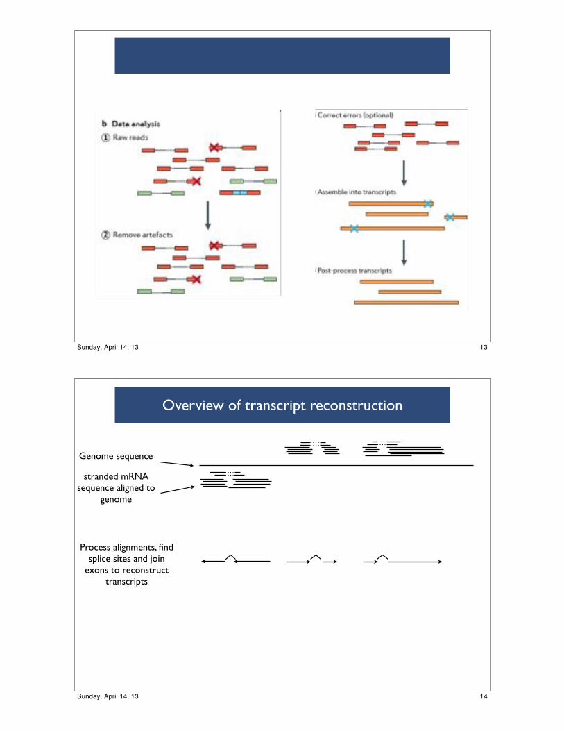
Overview of transcript reconstruction

Genome sequence

stranded mRNA sequence aligned to

genome

Process alignments, find splice sites and join

exons to reconstruct transcripts


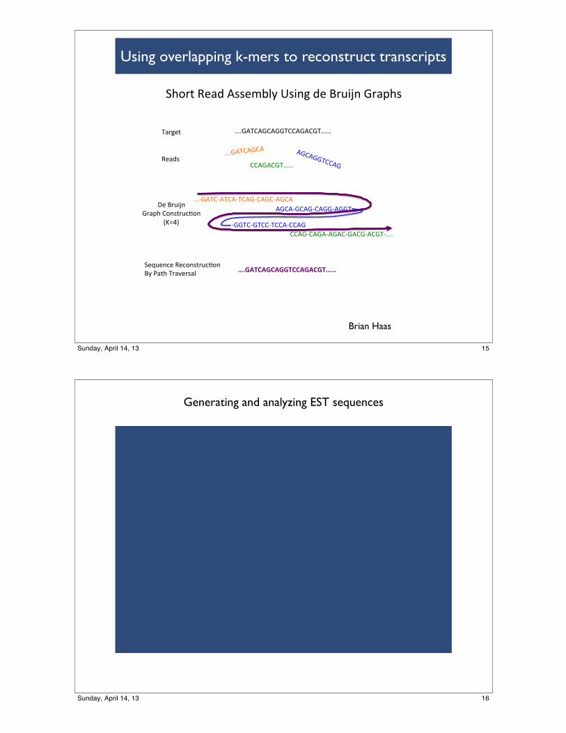
Using overlapping k-mers to reconstruct transcripts

!"#$%&'()*&+,,(-./0&1,234&*(&5$6273&8$)9",&

:;8+<=+8=+88<==+8+=8<::&

:;8+<=+8=+& +8=+88<==+8&==+8+=8<::&

:>8+<=>+<=+><=+8>=+8=>+8=+&+8=+>8=+8>=+88>+88<&

==+8>=+8+>+8+=>8+=8>+=8<>:;&>88<=>8<==><==+>==+8&

?(&5$6273&&8$)9"&=#3,%$6@A#3&

BCDEF&

!(G6(3@(&'(@#3,%$6@A#3&50&H)%"&<$)I($,)/& !"#$%&$#&$##%&&$#$&#%!!'

<)$4(%&

'()*,&

Brian Haas


Generating and analyzing EST sequences


Sequences obtained for the cassava genome

represented in an assembly of publicly available cassava ESTsequences (http://cassava.igs.umaryland.edu/blast/db/EST_asmbl_and_single.fasta), 96% can be mapped to thegenome assembly. It can be estimated that the remainingportion of the genome is largely repetitive and non-gene-coding. Consistent with this, the fractions of the estimatedgenome size (~31%) and WGS reads (~36%) that do notappear in the assembly are approximately equal, despite lowread error rates. The scaffolds obtained have yet to be assignedto chromosomes, as this requires genetic markers with knownsequence. However, an 88% complete genetic map comprising

23-linkage groups includes the genetic locations of 284 scaf-folds (Sraphet et al. 2011).

With the gene-rich portion of the genome in hand, thenext step is to identify the protein-coding genes and theexons that comprise them. This is achieved computationallyby aligning sequences from mRNA fragments (ESTs) to thegenome, as well as looking for regions with homology toknown proteins from other plant species. The 80,459 SangerESTs from Genbank were augmented by a new set of 2.7million reads from leaf and root libraries, generated by 454Life Sciences using the FLX Titanium platform. While half

b

aFig. 1 a Overview of wholegenome shotgun sequencingand assembly. Starting withplant material, many genomes’worth of DNA is extracted,purified, fragmented, pooledby length and sequenced to ahigh level of redundancy withthe aim of sequencing everyregion of the genome so that thechromosomal sequence canbe generated (assembled) byoverlapping fragments thathave (near-)identical sequences.Longer range, paired-end se-quence information is used tobridge sections of the genomethat are not unique (repeats) andimpossible to resolve by thisapproach b The phytozomegenome browser (http://www.phytozome.net/cassava)provides a portal for accessing,browsing, searching anddownloading all available cas-sava sequence and annotationdata and for comparative plantgenomic analysis

Table 1 Cassava genomic and mRNA sequence data

Sequence type Source Technology Sequencesgenerated

Notes

Genome shotgun Roche 454 Titanium 39,259,112

454 FLX Plus (experimental) 10,785,244

JGI 454 Titanium 21,581,680

Sanger 723,958

U. Maryland & UC Davis Sanger 75,748 BAC-end seq.

Expressed sequence tags (ESTs) Roche 454 Titanium 1.51 M reads (leaf) 0.30 M after removingchloroplast and rDNAsequences

454 Titanium 1.19 M reads (root)

various Sanger 80,459

Tropical Plant Biol. (2012) 5:88–94 91


ESTs in cassava

• 80,459 ESTs from Manihot esculenta from GenBank database

• Roche 454 sequenced leaf EST library highly redundant

• 1,512,780 reads -> filtered -> 299,509

• Take 10,000 random sequences and group with blastclust 50% length 95% ID

• Four commonest clusters include 30% of reads

• BLASTN &/or TBLASTN a few sequences from each cluster against nr

• Remove 30-50% of ESTS with homology to 18S, 26S rDNA

• seqclean removes short, low-complexity sequences, vector etc

• 1,187,328 root ESTs from 454

gene % EST reads

26S rDNA 48%

18S rDNA 18%

chloroplast 8.5%

Highly redundant leaf EST lib


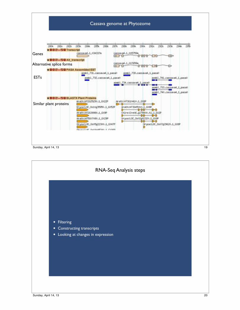
Cassava genome at Phytozome

ESTs

Genes

Alternative splice forms

Similar plant proteins


RNA-Seq Analysis steps

• Filtering

• Constructing transcripts

• Looking at changes in expression


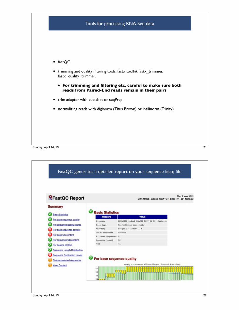
Tools for processing RNA-Seq data

• fastQC

• trimming and quality filtering tools: fastx toolkit fastx_trimmer, fastx_quality_trimmer.

• For trimming and filtering etc, careful to make sure both reads from Paired-End reads remain in their pairs

• trim adapter with cutadapt or seqPrep

• normalizing reads with diginorm (Titus Brown) or insilinorm (Trinity)


FastQC generates a detailed report on your sequence fastq file


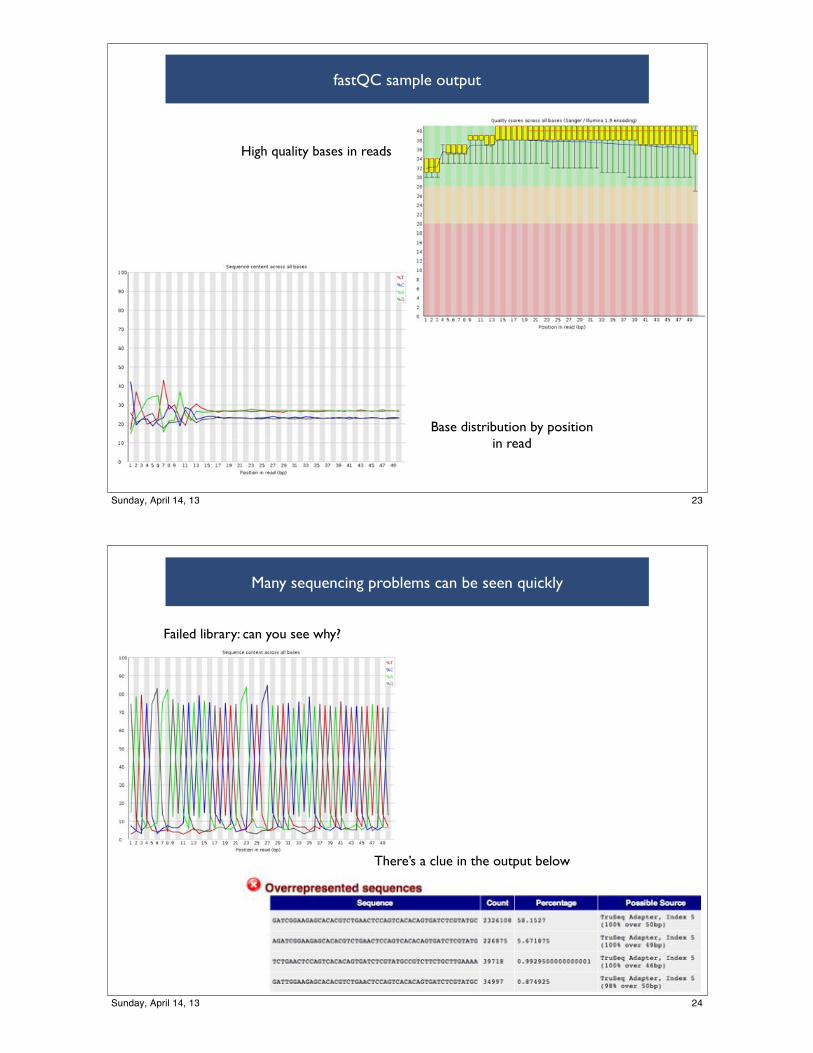
fastQC sample output

Base distribution by position in read

High quality bases in reads


Many sequencing problems can be seen quickly

Failed library: can you see why?

There’s a clue in the output below


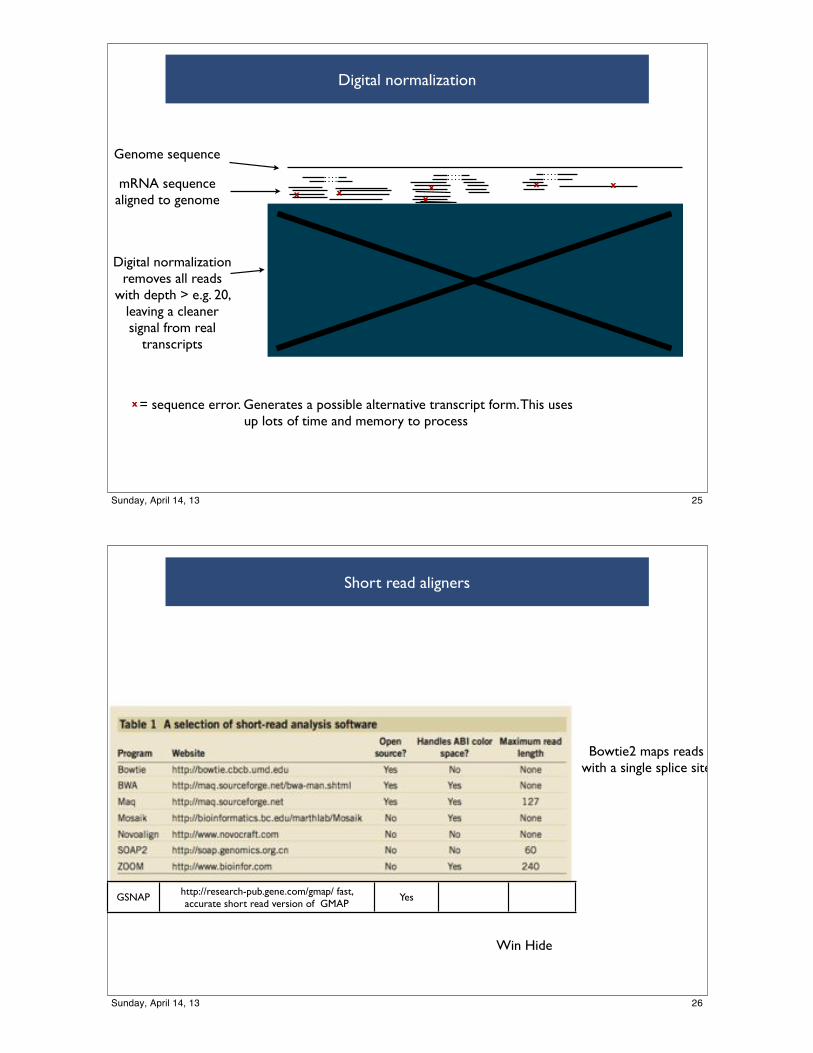
Digital normalization

Genome sequence

mRNA sequence aligned to genome x

x

x

x

x

x

x

xx

xx x

xx x x

= sequence error. Generates a possible alternative transcript form. This uses up lots of time and memory to process

x

Digital normalization removes all reads

with depth > e.g. 20, leaving a cleaner signal from real

transcripts


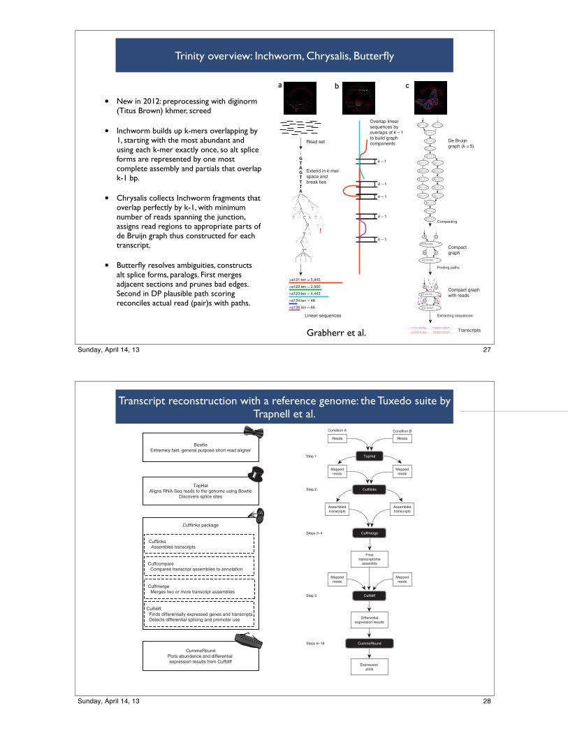
Short read aligners

Win Hide

Bowtie2 maps reads with a single splice site

GSNAP http://research-pub.gene.com/gmap/ fast, accurate short read version of GMAP

Yes


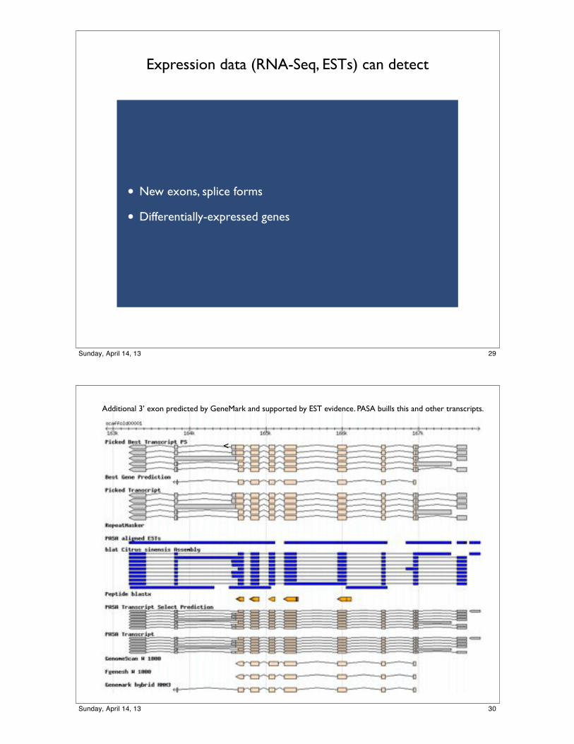
Trinity overview: Inchworm, Chrysalis, Butterfly

• New in 2012: preprocessing with diginorm (Titus Brown) khmer, screed

• Inchworm builds up k-mers overlapping by 1, starting with the most abundant and using each k-mer exactly once, so alt splice forms are represented by one most complete assembly and partials that overlap k-1 bp.

• Chrysalis collects Inchworm fragments that overlap perfectly by k-1, with minimum number of reads spanning the junction, assigns read regions to appropriate parts of de Bruijn graph thus constructed for each transcript.

• Butterfly resolves ambiguities, constructs alt splice forms, paralogs. First merges adjacent sections and prunes bad edges. Second in DP plausible path scoring reconciles actual read (pair)s with paths.

2 ADVANCE ONLINE PUBLICATION NATURE BIOTECHNOLOGY

complexity of overlaps between variants. Finally, Butterfly (Fig. 1c) analyzes the paths taken by reads and read pairings in the context of the corresponding de Bruijn graph and reports all plausible transcript sequences, resolving alternatively spliced isoforms and transcripts derived from paralogous genes. Below, we describe each of Trinity’s modules.

Inchworm assembles contigs greedily and efficientlyInchworm efficiently reconstructs linear transcript contigs in six steps (Fig. 1a). Inchworm (i) constructs a k-mer dictionary from all sequence reads (in practice, k = 25); (ii) removes likely error-containing k-mers from the k-mer dictionary; (iii) selects the most frequent k-mer in the dictionary to seed a contig assembly, excluding both low-complexity

For transcriptome assembly, each path in the graph represents a possible transcript. A scoring scheme applied to the graph structure can rely on the original read sequences and mate-pair information to discard non-sensical solutions (transcripts) and compute all plausible ones.

Applying the scheme of de Bruijn graphs to de novo assembly of RNA-Seq data represents three critical challenges: (i) efficiently construct-ing this graph from large amounts (billions of base pairs) of raw data; (ii) defining a suitable scoring and enumeration algorithm to recover all plausible splice forms and paralogous transcripts; and (iii) providing robustness to the noise stemming from sequencing errors and other artifacts in the data. In particular, sequencing errors would introduce a large number of false nodes, resulting in a massive graph with millions of possible (albeit mostly implausible) paths.

Here, we present Trinity, a method for the efficient and robust de novo reconstruction of transcriptomes, consisting of three software modules: Inchworm, Chrysalis and Butterfly, applied sequentially to process large volumes of RNA-Seq reads. We evaluated Trinity on data from two well-annotated species—one microorganism (fission yeast) and one mam-mal (mouse)—as well as an insect (the whitefly Bemisia tabaci), whose genome has not yet been sequenced. In each case, Trinity recovers most of the reference (annotated) expressed tran-scripts as full-length sequences, and resolves alternative isoforms and duplicated genes, per-forming better than other available transcrip-tome de novo assembly tools, and similarly to methods relying on genome alignments.

RESULTSTrinity: a method for de novo transcriptome assemblyIn contrast to de novo assembly of a genome, where few large connected sequence graphs can represent connectivities among reads across entire chromosomes, in assembling transcriptome data we expect to encounter numerous individual disconnected graphs, each representing the transcriptional com-plexity at nonoverlapping loci. Accordingly, Trinity partitions the sequence data into these many individual graphs, and then processes each graph independently to extract full-length isoforms and tease apart transcripts derived from paralogous genes.

In the first step in Trinity, Inchworm assembles reads into the unique sequences of transcripts. Inchworm (Fig. 1a) uses a greedy k-mer–based approach for fast and efficient transcript assembly, recovering only a single (best) representative for a set of alternative variants that share k-mers (owing to alterna-tive splicing, gene duplication or allelic varia-tion). Next, Chrysalis (Fig. 1b) clusters related contigs that correspond to portions of alterna-tively spliced transcripts or otherwise unique portions of paralogous genes. Chrysalis then constructs a de Bruijn graph for each cluster of related contigs, each graph reflecting the

cba

>a121:len = 5,845

>a122:len = 2,560

>a123:len = 4,443

>a124:len = 48

>a126:len = 66

k – 1

Read set

Extend in k-merspace andbreak ties

Linear sequences

...

!

A

A

A A

A

CGT

CTC

G

TCGT

T C

T G

T C

T* C

... ... ......

Overlap linearsequences byoverlaps of k – 1to build graphcomponents

De Bruijngraph (k = 5)

Compactgraph

Compact graphwith reads

Transcripts

Compacting

Finding paths

Extracting sequences

ATTCG CTTCG

TTCGC

TCGCA

CGCAA

GCAAT

CAATG CAATC

AATGA AATCA

ATGAT ATCAT

TGATC TCATC

GATCG CATCG

ATCGG

TCGGA

CGGAT

... ...

A C

TTCGCAA...T

ATCGGAT...

CG

... ...

A C

CG

... ...

...CTTCGCAA...TGATCGGAT...

...ATTCGCAA...TCATCGGAT...

k – 1

k – 1

k – 1

k – 1

TTCGCAA...T

ATCGGAT...

Figure 1 Overview of Trinity. (a) Inchworm assembles the read data set (short black lines, top) by greedily searching for paths in a k-mer graph (middle), resulting in a collection of linear contigs (color lines, bottom), with each k-mer present only once in the contigs. (b) Chrysalis pools contigs (colored lines) if they share at least one k – 1-mer and if reads span the junction between contigs, and then it builds individual de Bruijn graphs from each pool. (c) Butterfly takes each de Bruijn graph from Chrysalis (top), and trims spurious edges and compacts linear paths (middle). It then reconciles the graph with reads (dashed colored arrows, bottom) and pairs (not shown), and outputs one linear sequence for each splice form and/or paralogous transcript represented in the graph (bottom, colored sequences).

ART ICL ES

Grabherr et al.


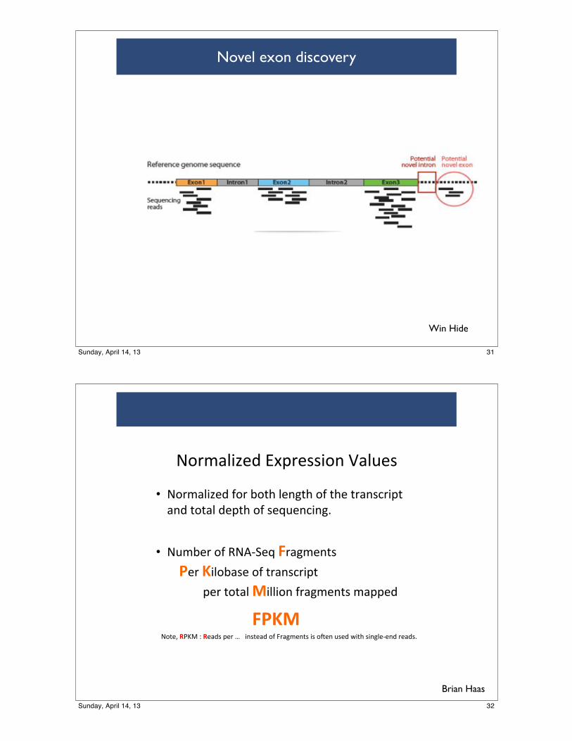
Transcript reconstruction with a reference genome: the Tuxedo suite by Trapnell et al.

©20

12 N

atur

e A

mer

ica,

Inc.

All

righ

ts r

eser

ved.

PROTOCOL

564 | VOL.7 NO.3 | 2012 | NATURE PROTOCOLS

feel comfortable creating directories, moving files between them and editing text files in a UNIX environment. Installation of the tools may require additional expertise and permission from one’s computing system administrators.

Read alignment with TopHatAlignment of sequencing reads to a reference genome is a core step in the analysis workflows for many high-throughput sequencing assays, including ChIP-Seq31, RNA-seq, ribosome profiling32 and others. Sequence alignment itself is a classic problem in computer science and appears frequently in bioinformatics. Hence, it is per-haps not surprising that many read alignment programs have been developed within the last few years. One of the most popular and to date most efficient is Bowtie33 (http://bowtie-bio.sourceforge.net/index.shtml), which uses an extremely economical data structure called the FM index34 to store the reference genome sequence and allows it to be searched rapidly. Bowtie uses the FM index to align reads at a rate of tens of millions per CPU hour. However, Bowtie is not suitable for all sequence alignment tasks. It does not allow alignments between a read and the genome to contain large gaps; hence, it cannot align reads that span introns. TopHat was created to address this limitation.

TopHat uses Bowtie as an alignment ‘engine’ and breaks up reads that Bowtie cannot align on its own into smaller pieces called seg-ments. Often, these pieces, when processed independently, will align to the genome. When several of a read’s segments align to the genome far apart (e.g., between 100 bp and several hundred kilobases) from one another, TopHat infers that the read spans a splice junction and estimates where that junction’s splice sites are. By processing each ‘initially unmappable’ read, TopHat can build up an index of splice sites in the transcriptome on the fly without a priori gene or splice site annotations. This capability is crucial, because, as numerous RNA-seq studies have now shown, our cata-logs of alternative splicing events remain woefully incomplete. Even in the transcriptomes of often-studied model organisms, new splic-ing events are discovered with each additional RNA-seq study.

Aligned reads say much about the sample being sequenced. Mismatches, insertions and deletions in the alignments can iden-tify polymorphisms between the sequenced sample and the ref-erence genome, or even pinpoint gene fusion events in tumor samples. Reads that align outside annotated genes are often strong evidence of new protein-coding genes and noncoding RNAs. As mentioned above, RNA-seq read alignments can reveal new alter-native splicing events and isoforms. Alignments can also be used to accurately quantify gene and transcript expression, because the number of reads produced by a transcript is proportional to its abundance (Box 2). Discussion of polymorphism and fusion

detection is out of the scope of this protocol, and we address transcript assembly and gene discovery only as they relate to dif-ferential expression analysis. For a further review of these topics, see Garber et al.12.

Transcript assembly with CufflinksAccurately quantifying the expression level of a gene from RNA-seq reads requires accurately identifying which isoform of a given gene produced each read. This, of course, depends on knowing all of the splice variants (isoforms) of that gene. Attempting to quantify gene and transcript expression by using an incomplete or incorrect transcriptome annotation leads to inaccurate expression values8. Cufflinks assembles individual transcripts from RNA-seq reads that have been aligned to the genome. Because a sample may contain reads from multiple splice variants for a given gene, Cufflinks must be able to infer the splicing structure of each gene. However, genes sometimes have multiple alternative splicing events, and there may be many possible reconstructions of the gene model that explain the sequencing data. In fact, it is often not obvious how many splice variants of the gene may be present. Thus, Cufflinks reports a parsi-monious transcriptome assembly of the data. The algorithm reports as few full-length transcript fragments or ‘transfrags’ as are needed to ‘explain’ all the splicing event outcomes in the input data.

TopHat

Cufflinks

Cuffmerge

Finaltranscriptome

assembly

Condition A

Reads

Mappedreads

Assembledtranscripts

Mappedreads

Condition B

Differentialexpression results

Cuffdiff

Expression plots

CummeRbund

Reads

Mappedreads

Assembledtranscripts

Mappedreads

Step 1

Step 2

Steps 3–4

Step 5

Steps 6–18

Figure 2 | An overview of the Tuxedo protocol. In an experiment involving two conditions, reads are first mapped to the genome with TopHat. The reads for each biological replicate are mapped independently. These mapped reads are provided as input to Cufflinks, which produces one file of assembled transfrags for each replicate. The assembly files are merged with the reference transcriptome annotation into a unified annotation for further analysis. This merged annotation is quantified in each condition by Cuffdiff, which produces expression data in a set of tabular files. These files are indexed and visualized with CummeRbund to facilitate exploration of genes identified by Cuffdiff as differentially expressed, spliced, or transcriptionally regulated genes. FPKM, fragments per kilobase of transcript per million fragments mapped.

©20

12 N

atur

e A

mer

ica,

Inc.

All

righ

ts r

eser

ved.

PROTOCOL

NATURE PROTOCOLS | VOL.7 NO.3 | 2012 | 563

TopHat and Cufflinks are both operated through the UNIX shell. No graphical user interface is included. However, there are now commercial products and open-source interfaces to these and other RNA-seq analysis tools. For example, the Galaxy Project18 uses a web interface to cloud computing resources to bring command-line–driven tools such as TopHat and Cufflinks to users without UNIX skills through the web and the computing cloud.

Alternative analysis packagesTopHat and Cufflinks provide a complete RNA-seq workflow, but there are other RNA-seq analysis packages that may be used instead of or in combination with the tools in this protocol. Many alterna-tive read-alignment programs19–21 now exist, and there are several alternative tools for transcriptome reconstruction22,23, quantifica-tion10,24,25 and differential expression26–28 analysis. Because many of these tools operate on similarly formatted data files, they could be used instead of or in addition to the tools used here. For example, with straightforward postprocessing scripts, one could provide GSNAP19 read alignments to Cufflinks, or use a Scripture22 tran-scriptome reconstruction instead of a Cufflinks one before differ-ential expression analysis. However, such customization is beyond the scope of this protocol, and we discourage novice RNA-seq users from making changes to the protocol outlined here.

This protocol is appropriate for RNA-seq experiments on organ-isms with sequenced reference genomes. Users working without a sequenced genome but who are interested in gene discovery should consider performing de novo transcriptome assembly using one of several tools such as Trinity29, Trans-Abyss30 or Oases (http://www.ebi.ac.uk/~zerbino/oases/). Users performing expression ana-lysis with a de novo transcriptome assembly may wish to consider RSEM10 or IsoEM25. For a survey of these tools (including TopHat and Cufflinks) readers may wish to see the study by Garber et al.12, which describes their comparative advantages and disadvantages and the theoretical considerations that inform their design.

Overview of the protocolAlthough RNA-seq experiments can serve many purposes, we describe a workflow that aims to compare the transcriptome pro-files of two or more biological conditions, such as a wild-type versus mutant or control versus knockdown experiments. For simplicity, we assume that the experiment compares only two biological con-ditions, although the software is designed to support many more, including time-course experiments.

This protocol begins with raw RNA-seq reads and concludes with publication-ready visualization of the analysis. Figure 2 highlights the main steps of the protocol. First, reads for each condition are mapped to the reference genome with TopHat. Many RNA-seq users are also interested in gene or splice variant discovery, and the failure to look for new transcripts can bias expression estimates and reduce accuracy8. Thus, we include transcript assembly with

Cufflinks as a step in the workflow (see Box 1 for a workflow that skips gene and transcript discovery). After running TopHat, the resulting alignment files are provided to Cufflinks to generate a transcriptome assembly for each condition. These assemblies are then merged together using the Cuffmerge utility, which is included with the Cufflinks package. This merged assembly provides a uni-form basis for calculating gene and transcript expression in each condition. The reads and the merged assembly are fed to Cuffdiff, which calculates expression levels and tests the statistical signifi-cance of observed changes. Cuffdiff also performs an additional layer of differential analysis. By grouping transcripts into biologi-cally meaningful groups (such as transcripts that share the same transcription start site (TSS)), Cuffdiff identifies genes that are dif-ferentially regulated at the transcriptional or post-transcriptional level. These results are reported as a set of text files and can be displayed in the plotting environment of your choice.

We have recently developed a powerful plotting tool called CummeRbund (http://compbio.mit.edu/cummeRbund/), which provides functions for creating commonly used expression plots such as volcano, scatter and box plots. CummeRbund also han-dles the details of parsing Cufflinks output file formats to con-nect Cufflinks and the R statistical computing environment. CummeRbund transforms Cufflinks output files into R objects suitable for analysis with a wide variety of other packages available within the R environment and can also now be accessed through the Bioconductor website (http://www.bioconductor.org/).

This protocol does not require extensive bioinformatics exper-tise (e.g., the ability to write complex scripts), but it does assume familiarity with the UNIX command-line interface. Users should

Cufflinks package

Cuffcompare Compares transcript assemblies to annotation

Cuffmerge Merges two or more transcript assemblies

Cuffdiff Finds differentially expressed genes and transcripts Detects differential splicing and promoter use

TopHatAligns RNA-Seq reads to the genome using Bowtie

Discovers splice sites

CummeRbundPlots abundance and differential expression results from Cuffdiff

BowtieExtremely fast, general purpose short read aligner

Cufflinks Assembles transcripts

Figure 1 | Software components used in this protocol. Bowtie33 forms the algorithmic core of TopHat, which aligns millions of RNA-seq reads to the genome per CPU hour. TopHat’s read alignments are assembled by Cufflinks and its associated utility program to produce a transcriptome annotation of the genome. Cuffdiff quantifies this transcriptome across multiple conditions using the TopHat read alignments. CummeRbund helps users rapidly explore and visualize the gene expression data produced by Cuffdiff, including differentially expressed genes and transcripts.


Expression data (RNA-Seq, ESTs) can detect

• New exons, splice forms

• Differentially-expressed genes


<

Additional 3’ exon predicted by GeneMark and supported by EST evidence. PASA buills this and other transcripts.


Novel exon discovery

some slides from Win

Win Hide


!"#$%&'()*+,-.#)//'"0+1%&2)/++•  !"#$%&'()*+3"#+4"56+&)0756+"3+56)+5#%0/8#'.5+%0*+5"5%&+*).56+"3+/)92)08'07:+

•  !2$4)#+"3+;!<=>)9+!#%7$)05/++++++")#+#'&"4%/)+"3+5#%0/8#'.5+++++++++++++.)#+5"5%&+$'&&'"0+3#%7$)05/+$%..)*+

!"#$%!"5)?+&@AB+C+&)%*/+.)#+D+++'0/5)%*+"3+E#%7$)05/+'/+"F)0+2/)*+G'56+/'07&)=)0*+#)%*/:+

Brian Haas


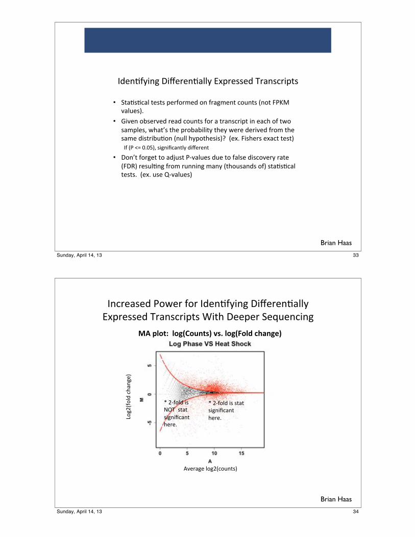
!"#$%&'($)*+(,#-#$%.//'*012-#33#"*4-.$35-(263*

•  76.%3%5./*6#363*2#-&8-9#"*8$*&-.)9#$6*58:$63*;$86*<=>?*@./:#3AB*

•  C(@#$*8D3#-@#"*-#."*58:$63*&8-*.*6-.$35-(26*($*#.5E*8&*6F8*3.92/#3G*FE.6H3*6E#*2-8D.D(/(6'*6E#'*F#-#*"#-(@#"*&-89*6E#*3.9#*"(36-(D:%8$*;$://*E'286E#3(3AI**;#1B*<(3E#-3*#1.56*6#36A*!&*;=*JK*LBLMAG*3()$(N5.$6/'*"(,#-#$6*

•  +8$H6*&8-)#6*68*."O:36*=P@./:#3*":#*68*&./3#*"(358@#-'*-.6#*;<+QA*-#3:/%$)*&-89*-:$$($)*9.$'*;6E8:3.$"3*8&A*36.%3%5./*6#363B**;#1B*:3#*RP@./:#3A*

Brian Haas


!"#$%&'%()*+,%$)-+$)!(%".-/0"1)203%$%".&44/)

567$%''%()8$&"'#$079'):09;)2%%7%$)<%=>%"#0"1)

?+1@A-+4()#;&"1%B)

CD%$&1%)4+1@A#+>"9'B)

!"#$%&'(##%&)*+&,-'./#0.1#%&)*2&%3#456-)7/#

E)@F-+4()0')'9&9)'01"0G#&"9)

;%$%H)

E)@F-+4()0')IJ8))'9&9)

'01"0G#&"9);%$%H)

Brian Haas


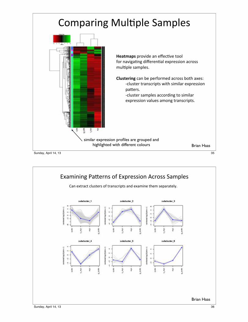
!"#$%&'()*+,-.$-/*0%#$-/1*

!"#$%#&'*$&"2'3/*%(*/4/5.2/*6""-*7"&*(%2')%.()*3'4/&/(.%-*/8$&/11'"(*%5&"11*#,-.$-/*1%#$-/19**()*'$"+,-.*5%(*:/*$/&7"&#/3*%5&"11*:"6;*%8/1<*

*=5-,16/&*6&%(15&'$61*>'6;*1'#'-%&*/8$&/11'"(**$%?/&19**=5-,16/&*1%#$-/1*%55"&3'()*6"*1'#'-%&**/8$&/11'"(*2%-,/1*%#"()*6&%(15&'$619***

Brian Haassimilar expression profiles are grouped and

highlighted with different colours


!"#$%&%&'()#*+,&-(./(!"0,+--%.&(12,.--(3#$04+-(5#&(+"6,#26(247-6+,-(./(6,#&-2,%06-(#&8(+"#$%&+(69+$(-+0#,#6+4:;(

Brian Haas


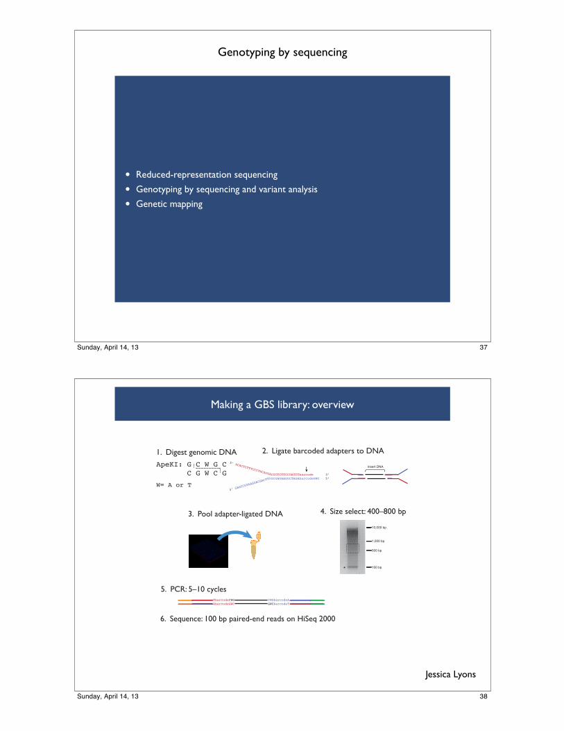
Genotyping by sequencing

• Reduced-representation sequencing

• Genotyping by sequencing and variant analysis

• Genetic mapping


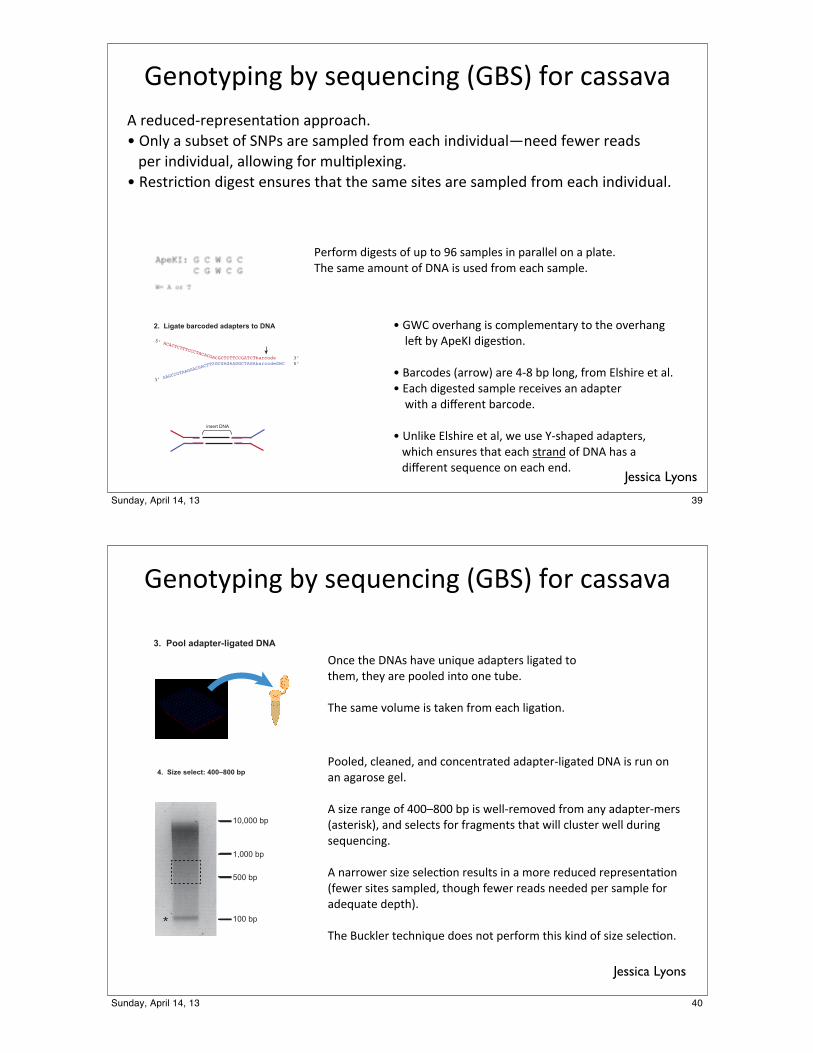
Making a GBS library: overview

ApeKI: G C W G C C G W C G

W= A or T

1. Digest genomic DNA

3. Pool adapter-ligated DNA 4. Size select: 400–800 bp

5. PCR: 5–10 cyclesTbarcodeCWG CWGbarcodeAAbarcodeGWC GWCbarcodeT

6. Sequence: 100 bp paired-end reads on HiSeq 2000

5’ ACACTCTTTCCCTACACGA

3’ GAGCC

GTAAGGAC

GACTTG

!"#$%&'()*

CGCTCTTCCGATCTbarcode 3’GCGAGAAGGCTAGAbarcodeGWC 5’

+,-,,,'./

0,,'./

+,,'./

+-,,,'./

1

2. Ligate barcoded adapters to DNA

Jessica Lyons


!"#$%&'(#)*+&*,"-."#/(#)*0!123*4$5*/6,,6768*5"9./"9:5"'5","#%6;$#*6''5$6/<=>*?#@&*6*,.+,"%*$4*2AB,*65"*,6C'@"9*45$C*"6/<*(#9(7(9.6@D#""9*4"E"5*5"69,****'"5*(#9(7(9.6@F*6@@$E(#)*4$5*C.@;'@"G(#)=>*H",%5(/;$#*9()",%*"#,.5",*%<6%*%<"*,6C"*,(%",*65"*,6C'@"9*45$C*"6/<*(#9(7(9.6@=

B"54$5C*9()",%,*$4*.'*%$*IJ*,6C'@",*(#*'656@@"@*$#*6*'@6%"=K<"*,6C"*6C$.#%*$4*LA8*(,*.,"9*45$C*"6/<*,6C'@"=

>*!MN*$7"5<6#)*(,*/$C'@"C"#%65&*%$*%<"*$7"5<6#)*****@"O*+&*8'"PQ*9()",;$#=

>*165/$9",*0655$E3*65"*R:S*+'*@$#)F*45$C*T@,<(5"*"%*6@=>*T6/<*9()",%"9*,6C'@"*5"/"(7",*6#*696'%"5*****E(%<*6*9(U"5"#%*+65/$9"=

>*V#@(W"*T@,<(5"*"%*6@F*E"*.,"*X:,<6'"9*696'%"5,F****E<(/<*"#,.5",*%<6%*"6/<*,%56#9*$4*LA8*<6,*6****9(U"5"#%*,"-."#/"*$#*"6/<*"#9=

!"##$%&'()#*'+,-.).#'.'/()+0#(-#123

5’ ACACTCTTTCCCTACACGA

3’ GAGCC

GTAAGGAC

GACTTG

CGCTCTTCCGATCTbarcode 3’GCGAGAAGGCTAGAbarcodeGWC 5’

!"#$%&'()*

Jessica Lyons


!"#$%&'(#)*+&*,"-."#/(#)*0!123*4$5*/6,,676

?#/"*%<"*LA8,*<67"*.#(-."*696'%"5,*@()6%"9*%$*%<"CF*%<"&*65"*'$$@"9*(#%$*$#"*%.+"=

K<"*,6C"*[email protected]"*(,*%6W"#*45$C*"6/<*@()6;$#=

B$$@"9F*/@"6#"9F*6#9*/$#/"#%56%"9*696'%"5:@()6%"9*LA8*(,*5.#*$#*6#*6)65$,"*)"@=

8*,(Y"*56#)"*$4*RZZ[SZZ*+'*(,*E"@@:5"C$7"9*45$C*6#&*696'%"5:C"5,*06,%"5(,W3F*6#9*,"@"/%,*4$5*456)C"#%,*%<6%*E(@@*/@.,%"5*E"@@*9.5(#)*,"-."#/(#)=

8*#655$E"5*,(Y"*,"@"/;$#*5",.@%,*(#*6*C$5"*5"9./"9*5"'5","#%6;$#*04"E"5*,(%",*,6C'@"9F*%<$.)<*4"E"5*5"69,*#""9"9*'"5*,6C'@"*4$5*69"-.6%"*9"'%<3=

K<"*1./W@"5*%"/<#(-."*9$",*#$%*'"54$5C*%<(,*W(#9*$4*,(Y"*,"@"/;$#=

!"##$%%&#'(')*+,-&./'*+(#012

!"##$%&'#(')'*+,#!--./--#01

!"#"""$%&

'""$%&

!""$%&

!#"""$%&

(

Jessica Lyons


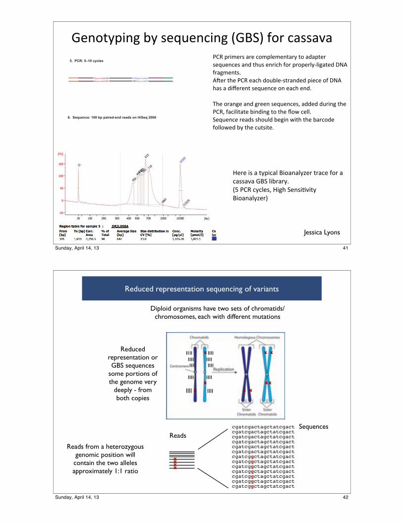
!"#$%&'(#)*+&*,"-."#/(#)*0!123*4$5*/6,,676BNH*'5(C"5,*65"*/$C'@"C"#%65&*%$*696'%"5*,"-."#/",*6#9*%<.,*"#5(/<*4$5*'5$'"5@&:@()6%"9*LA8*456)C"#%,=8O"5*%<"*BNH*"6/<*9$.+@":,%56#9"9*'("/"*$4*LA8*<6,*6*9(U"5"#%*,"-."#/"*$#*"6/<*"#9=**

K<"*$56#)"*6#9*)5""#*,"-."#/",F*699"9*9.5(#)*%<"*BNHF*46/(@(%6%"*+(#9(#)*%$*%<"*\$E*/"@@=2"-."#/"*5"69,*,<$.@9*+")(#*E(%<*%<"*+65/$9"*4$@@$E"9*+&*%<"*/.%,(%"=

]"5"*(,*6*%&'(/6@*1($6#6@&Y"5*%56/"*4$5*6*/6,,676*!12*@(+565&=0^*BNH*/&/@",F*]()<*2"#,(;7(%&*1($6#6@&Y"53

!"##$%&'#!()*#+,+-./

TbarcodeCWG CWGbarcodeAAbarcodeGWC GWCbarcodeT

!"##$%&'%()%*#+,,#-.#./01%23%(2#1%/24#5(#60$%&#7,,,

Jessica Lyons


Reduced representation sequencing of variants

Diploid organisms have two sets of chromatids/chromosomes, each with different mutations

xx

x

x

x

x

x

x x

Reduced representation or GBS sequences

some portions of the genome very

deeply - from both copies

xxxx

Reads from a heterozygous genomic position will contain the two alleles approximately 1:1 ratio

cgatcgactagctatcgactcgatcgactagctatcgactcgatcgactagctatcgactcgatcgactagctatcgactcgatcgactagctatcgactcgatcgactagctatcgactcgatcggctagctatcgactcgatcggctagctatcgactcgatcggctagctatcgactcgatcggctagctatcgactcgatcggctagctatcgactcgatcggctagctatcgactcgatcggctagctatcgact

ReadsSequences


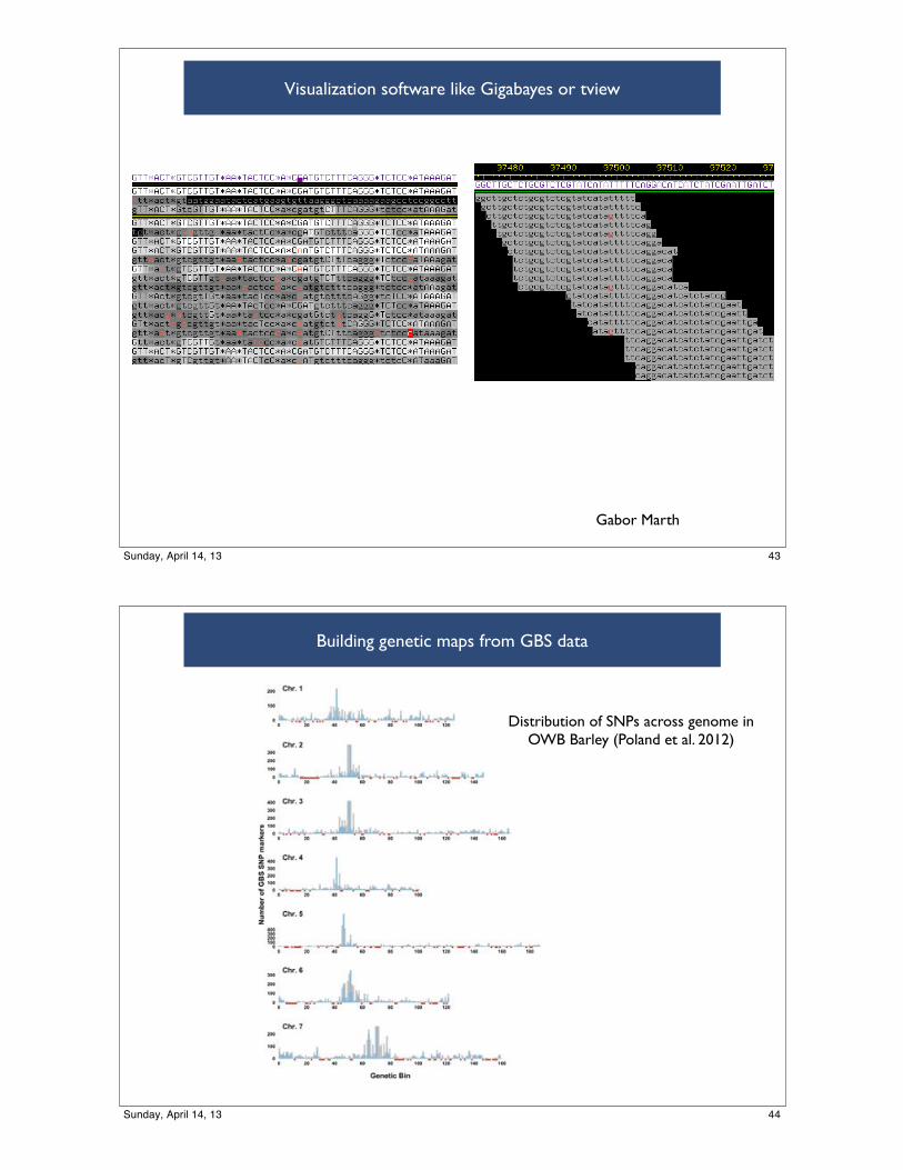
Visualization software like Gigabayes or tview

!"""#$%&'$()*$+,-./$0&123$4(55")6$

Gabor Marth


Building genetic maps from GBS data

Distribution of SNPs across genome in OWB Barley (Poland et al. 2012)


Building genetic maps from GBS data with JoinMap

JoinMap encoding of parental genotypes

lm x ll nn x np

Expected Genotype Frequencies in progeny

ll: 0.5

lm: 0.5

mm: 0.0

nn: 0.5

np: 0.5

pp: 0.0

chromosome position SNP type

chr1 354 lm

chr1 4983 lm

chr1 4985 lm

chr1 10876 ll

chr2 765 ll

chr2 1034526 lm

chr2 1034700 ll

chr3 45673 lm

etc

Example SNPs

A/G x A/A C/C x C/A

Data table encoding characters or markers for making the map


Genomic selection from GBS data

Phenotypic evaluation of cassava is a lengthy process

Make crosses: 10000’s of seedlings

5 to 10 best

500 to 3000 clones

20 to 25 clones

50 to 100 clones

Year 1

Year 2

Year 3

Year 4

Year 5

Year 6 5 best

Martha Hamblin

Evaluation at the Seedling Stageby Genomic Selection

Meuwissen et al. 2001:

Use genome-wide markers to capture effects at many (20-30k) loci

Develop a statistical model to predict breeding value

“Selection on genetic values predicted from markers could substantially increase the rate of genetic gain in animals and plants.”


Documents

Session 1b Applications, genome sequencing, RNA …cassavabase.wikispaces.com/file/view/Session1bSeqApplications_LQ...2003 Drosophila genome 250k Sanger ESTs 700 175 2005 ... With