Session 2, Tuesday, April 9th (10:30-11:45)

v2.0 © 2014 Association for Financial Professionals. All rights reserved. Session 12 - 1

Session 2, Tuesday, April 9th (10:30-11:45)Cost Accounting Topics: Variance Analysis


• Analyzing Information and Giving Feedback: Part II, Domain A, Chapter 7

Chapter Covered


Essential Aspects of Variance Analysis

• Key issue: How is the financial plan/model/business performing?

• Variance: Actual results minus projections

• Favorable or unfavorable? Depends on context


A company’s fiscal year is the calendar year. Total direct costs forecasted for a fiscal year are $150,000 and year-to-date direct costs at the end of March are $31,000. Calculate the direct cost variance if the spend rate remains unchanged throughout the year. Drop down choices are “favorable” and “unfavorable”

From the Candidate Guide: FP&A Sample Question on Variance Analysis


Answer

Answer: $26,000 Favorable

• Rationale: In order to arrive at the solution calculate the annualized amount of direct expenses based on the stated spend rate over the period given. Total direct expenses in 3 months are $31,000.

• Annualized direct expenses will be 12 / 3 x 31,000 = $124,000.

• $150,000-$124,000 = $26,000 Favorable.


Key Types of Variances

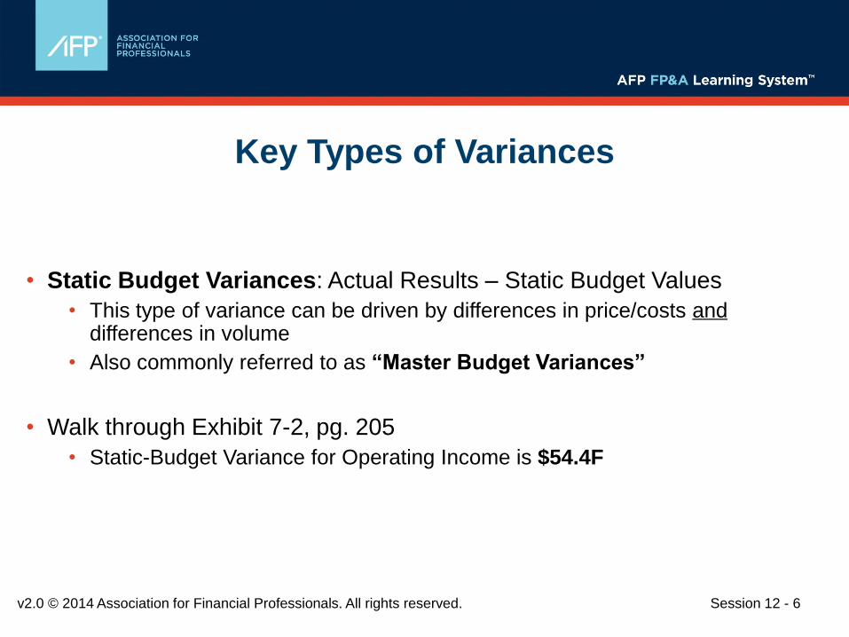
• Static Budget Variances: Actual Results – Static Budget Values

• This type of variance can be driven by differences in price/costs anddifferences in volume

• Also commonly referred to as “Master Budget Variances”

• Walk through Exhibit 7-2, pg. 205

• Static-Budget Variance for Operating Income is $54.4F


Key Types of Variances

• Flexible Budget Variances: Actual Results – Flexible Budget Values

• This type of variance is driven by differences in price/costs, not differences in volume

• Also commonly referred to as “Variable Budget Variances”

• Comment on the “relevant range”

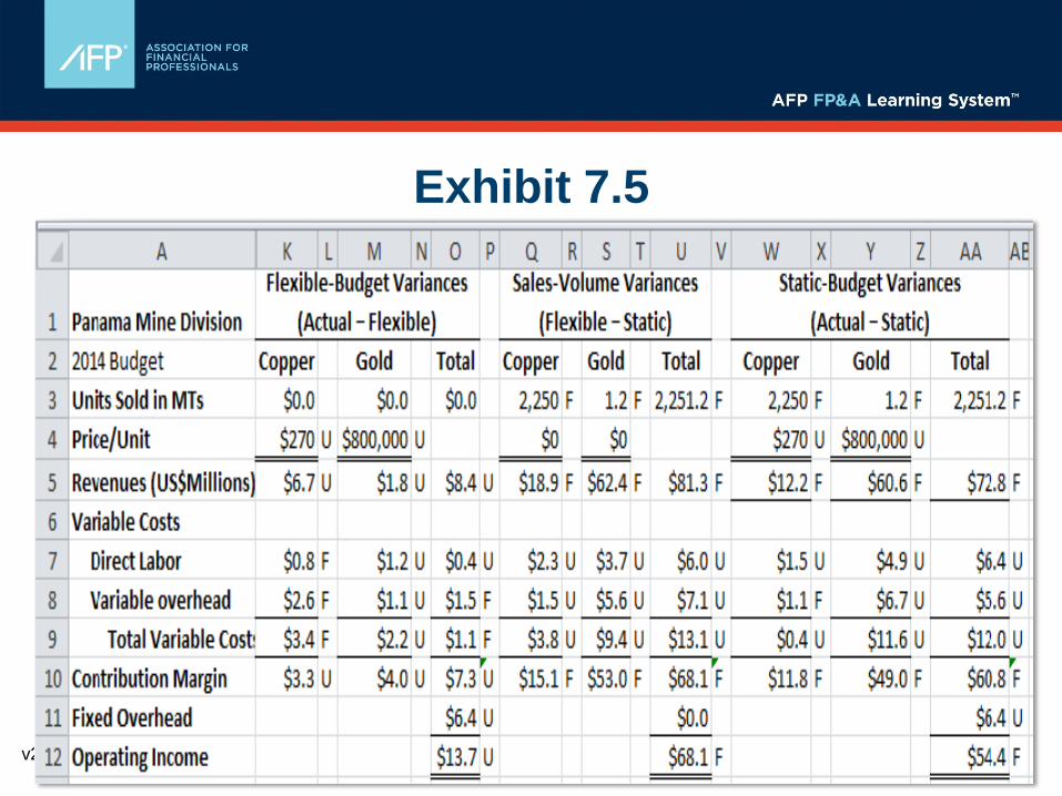
• Walk through Exhibit 7-5, pg. 208

• Flexible Budget Variance is $13.7U


Putting the Variances Together

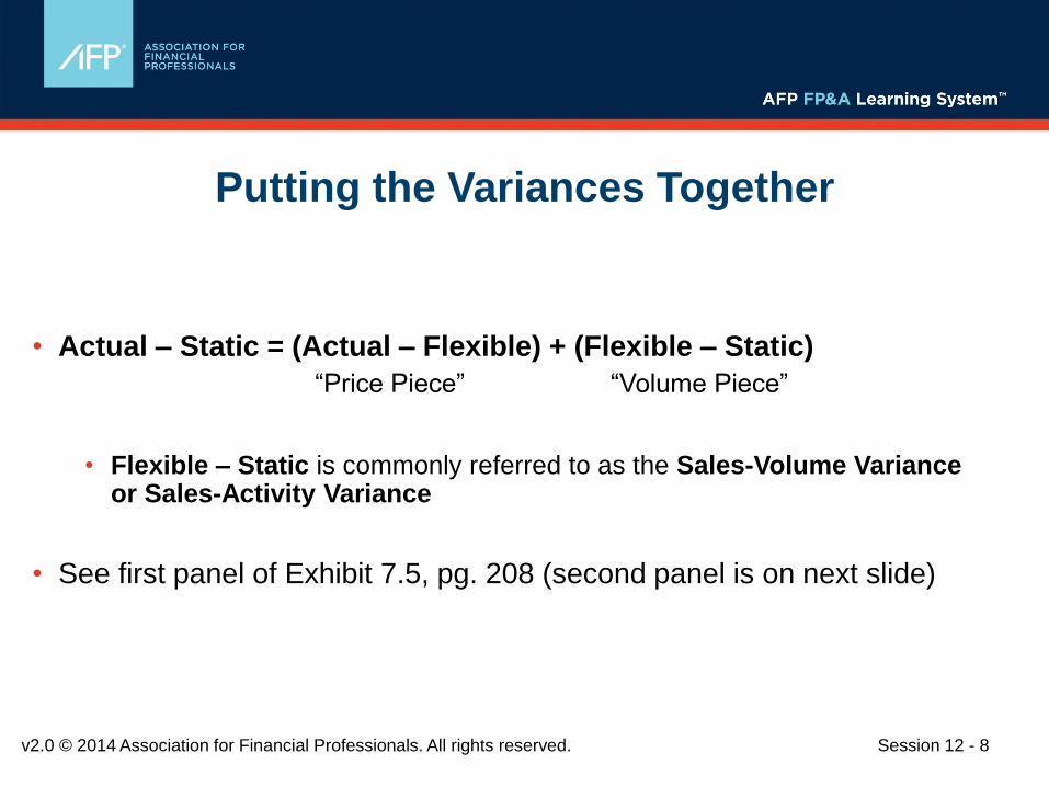
• Actual – Static = (Actual – Flexible) + (Flexible – Static)

“Price Piece” “Volume Piece”

• Flexible – Static is commonly referred to as the Sales-Volume Variance or Sales-Activity Variance

• See first panel of Exhibit 7.5, pg. 208 (second panel is on next slide)


Exhibit 7.5


Potential Root Causes: Sales Volume Variances


Integrated Problem

Assume the following values are used to develop a Static Budget:

• Units Sold 9,000

• Revenues of $279,000

• Variable Expenses of $196,200

• Fixed Expenses of $70,000


Integrated Problem

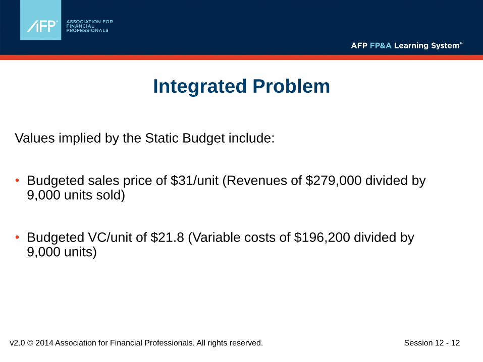
Values implied by the Static Budget include:

• Budgeted sales price of $31/unit (Revenues of $279,000 divided by 9,000 units sold)

• Budgeted VC/unit of $21.8 (Variable costs of $196,200 divided by 9,000 units)


Integrated Problem

Assume the following Actual Values:

• Units Sold 7,000

• Revenues of $217,000

• Sales price of $31/unit was earned

• Variable Expenses of $158,270

• VC per unit was $22.61 ($158,270/7,000)

• Fixed Expenses of $70,300


Static Budget Variances

Actuals Actuals Static Budget Variance

Revenues $217,000 $279,000 $62,000U

Variable Costs $158,270 $196,200 37,930F

Contribution Margin $58,730 $82,800 $24,070U

Fixed Costs $70,300 $70,000 $300U

Operating Income $(11,570) $12,800 $24,370U


Flexible Budget Variances

Actuals Actuals Flexible Budget Variance

Revenues $217,000 $217,000 $0

Variable Costs $158,270 $152,600 $5,670U

Contribution Margin $58,730 $64,400 $5,670U

Fixed Costs $70,300 $70,000 $300U

Operating Income $(11,570) $(5,600) $5,970U


Sales-Volume Variance

Actuals Flexible Budget Static Budget Variance

Revenues $217,000 $279,000 $62,000U

Variable Costs $152,600 $196,200 43,600F

Contribution Margin $64,400 $82,800 18,400U

Fixed Costs $70,000 $70,000 $0

Operating Income $(5,600) $12,800 $18,400U


Sales Volume Variance

Sales Volume Variance = Budgeted CM per Unit *(Static Budget Unit Sales – Actual Unit Sales)

= $9.2*(9,000 – 7,000) = $18,400U


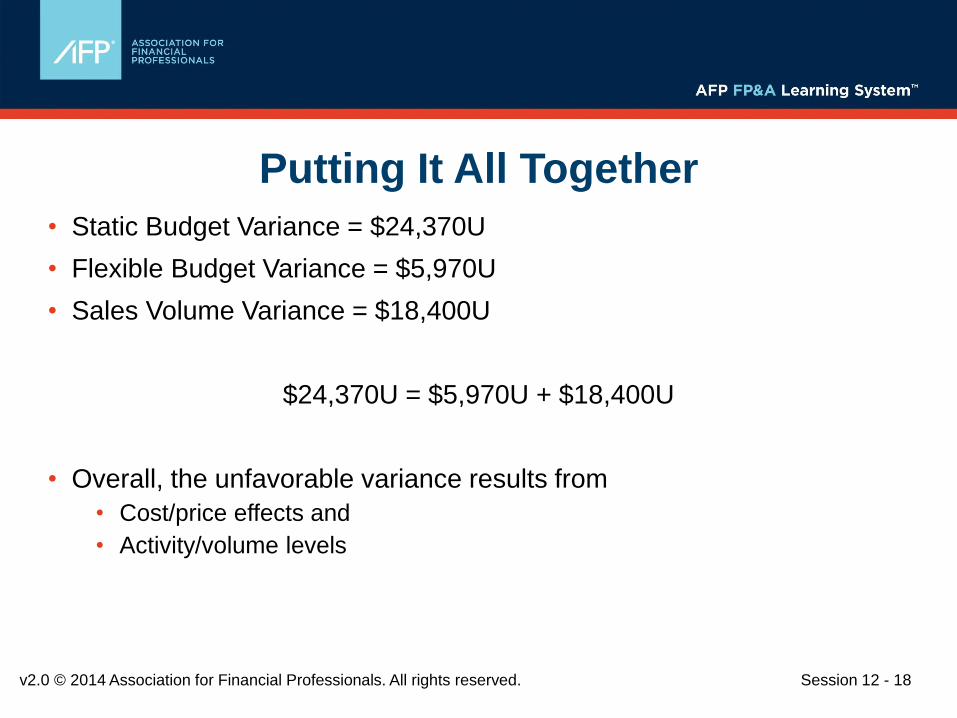
Putting It All Together

• Static Budget Variance = $24,370U

• Flexible Budget Variance = $5,970U

• Sales Volume Variance = $18,400U

$24,370U = $5,970U + $18,400U

• Overall, the unfavorable variance results from

• Cost/price effects and

• Activity/volume levels


More on Variances

Selling Price Variance:

(Actual Selling Price – Budgeted Selling Price)*Actual Units Sold

Price (of materials/labor) Variance:

(Actual Price of Input – Budgeted Price of Input)*Actual Quantity of Input

Efficiency Variance:

(Actual Quantity of Input – Budgeted Quantity of Input)*Budgeted Price of Input

• See pgs. 214, 217, and 218


Integrated Example

• To produce 7,000 units, suppose that 36,800 pounds of materials were purchased and used at an actual unit price of $1.90 for a total actual cost of $69,920

• Let’s develop the price and efficiency variances

Standard Inputs for each Unit of Output

Standard Price Expected for each Unit of Input

Direct Material 5 pounds $2 per pound


More on Variances

Price Variance:


= ($1.90 - $2) *36,800 = $3,680F



= (36,800 – 35,000)*$2 = $3,600U

Total Direct-Materials Flexible-Budget Variance = $80F


Integrated Example

• To produce 7,000 units, suppose that 3,750 hours were used at an actual hourly price of $16.40, for a total actual cost of $61,500

• Let’s develop the price and efficiency variances

Standard Inputs for

each Unit of Output

Standard Price Expected for

each Unit of Input

Direct Material 0.5 hours $16 per hour


More on Variances

Price Variance:


= ($16.40 - $16) *3,750 = $1,500U



= (3,750 – 3,500)*$16 = $4,000U

Total Direct-Labor Flexible-Budget Variance = $5,500U


Communicating the Materiality of Variances

• Waterfall chart

Documents

Session 2, Tuesday, April 9th (10:30-11:45)