Set characterizations and convex extensions for geometric

Mathematical Programminghttps://doi.org/10.1007/s10107-021-01705-3

FULL LENGTH PAPER

Series A

Set characterizations and convex extensions for geometricconvex-hull proofs

Andreas Bärmann1 ·Oskar Schneider2

Received: 20 January 2021 / Accepted: 13 August 2021© The Author(s) 2021

AbstractIn the present work, we consider Zuckerberg’s method for geometric convex-hullproofs introduced in Zuckerberg (Oper Res Lett 44(5):625–629, 2016). It has onlybeen scarcely adopted in the literature so far, despite the great flexibility in designingalgorithmic proofs for the completeness of polyhedral descriptions that it offers. Wesuspect that this is partly due to the rather heavy algebraic framework its original state-ment entails. This is whywe present a muchmore lightweight and accessible approachto Zuckerberg’s proof technique, building on ideas from Gupte et al. (Discrete Optim36:100569, 2020).We introduce the concept of set characterizations to replace the set-theoretic expressions needed in the original version and to facilitate the constructionof algorithmic proof schemes. Along with this, we develop several different strategiesto conduct Zuckerberg-type convex-hull proofs. Very importantly, we also show thatour concept allows for a significant extension of Zuckerberg’s proof technique. Whilethe original method was only applicable to 0/1-polytopes, our extended frameworkallows to treat arbitrary polyhedra and even general convex sets. We demonstrate thisincrease in expressive power by characterizing the convex hull of Boolean and bilinearfunctions over polytopal domains. All results are illustrated with indicative examplesto underline the practical usefulness and wide applicability of our framework.

Research reported in this paper was supported by the Bavarian Ministry of Economic Affairs, RegionalDevelopment and Energy through the Center for Analytics – Data – Applications (ADA-Center) withinthe framework of “BAYERN DIGITAL II”.

B Oskar [email protected]

Andreas Bä[email protected]

1 Department Mathematik, Friedrich-Alexander-Universität Erlangen-Nürnberg, Erlangen,Germany

2 Fraunhofer-Arbeitsgruppe für Supply-Chain Services SCS, Fraunhofer-Institut für IntegrierteSchaltungen IIS, Nuremberg, Germany

123

http://crossmark.crossref.org/dialog/?doi=10.1007/s10107-021-01705-3&domain=pdf

A. Bärmann, O. Schneider

Keywords Convex-hull proofs · Zuckerberg’s method · Proof-by-picture method ·Set characterizations · Integer polytopes

Mathematics Subject Classification 90C57 · 52B05 · 90C10 · 90C27 · 90C25

1 Introduction

Studying polyhedral structures lies at the heart of mixed-integer programming. It iswell-known to anyone in the field that a good understanding of the facial structure ofa given integer linear optimization problem both informs theory and practical algo-rithm development in a very beneficial way. This includes tight problem relaxations,extended formulations, cutting plane algorithms, only to name a few. A more or lesscomplete understanding of a polyhedron can be claimed if one accomplishes a so-called convex-hull proof, i.e. a proof that a given inequality description is sufficient todescribe its feasible set. The book [19] includes a popular list of possible approachesto obtain such a proof. They include total unimodularity, TDI-ness, projection or adirect proof that all vertices are integral, among a couple of others. For all of theseapproaches, there are numerous examples where they have been used successfully,and typically each of these methods works especially well for particular types of prob-lems (such as total unimodularity for network-type problems or TDI-ness for balancedmatrices)

A relatively new technique for convex-hull proofs has been given in [22] by Zucker-berg, with precursors in [1,16,21]. It is a geometric approach based on subset algebra.The core of Zuckerberg’s method is a novel type of criterion for showing that any givenpoint within a given polytope H (in H-description) lies within a second polytope P(in V-description), with the aim to show P = H . It works by giving an implicit (ratherthan an explicit), set-theoretic representation of this point as a convex combinationof the vertices of the latter. The actual proof takes the form of an algorithm whichcomputes such a set-theoretic representation. In contrast to other popular approaches,like TU or TDI, Zuckerberg’s method is constructive, in the sense that it is evenpossible to obtain an algorithm to compute the convex combination in explicit form.Zuckerberg himself refers to his method either as geometric convex-hull proofs or asthe proof-by-picture method, because this algorithm and its result can be visualized ina diagram incorporating all necessary information. For the sake of simplicity, we willuse the name Zuckerberg’s method throughout to refer to this technique as well as ourextensions of it.

Although the examples outlined in [22] already convey the impression of a verypowerful proof technique, it has only been scarcely adopted in the literature so far.We assume that this is due to the rather heavy algebraic framework that has been usedto derive and state the method. Zuckerberg has stated his method in terms of abstractmeasure spaces over which set-theoretic expressions have to be derived. In the recentwork [11], the authors give a significantly simplified version of his approach by passingover to a concrete measure space: a real interval equipped with the Lebesgue measure.Their actual aim in this article are proofs on the facial structure of the graphs ofbilinear functions. However, they also give a short introduction to his proof technique

123

Set characterizations and convex extensions for geometric…

and find a way to state it mostly without using set-algebraic terms. Afterwards, theyshow that their simplification of Zuckerberg’smethod allows for elegant proofs of theirstatements. In [12], the authors continue the work of [11] and give further convex-hull results on special graph classes. The authors of [6] have adopted their simplifiedapproach of Zuckerberg’s method in order to give convex-hull proofs for special casesof the Boolean quadric polytope (see [18]) with multiple-choice constraints.

In [1,21], the authors introduced the Bienstock–Zuckerberg hierarchy, which hassince then been simplified in [2,9]. As stated in [22], Zuckerberg’s method arose as aby-product of the analysis of this hierarchy in [21]. While the Bienstock–Zuckerberghierarchy itself entails a procedure to obtain increasingly tighter convex relaxationsfor integer sets, Zuckerberg’s method is an approach for proving the completeness ofconvex-hull descriptions. Our work builds upon the latter.

Contribution In the present article, we aim to show the power and flexibility ofZuckerberg’s approach to conduct convex-hull proofs. To this end, we give a conciseand accessible derivation of the technique and relate it to themethod in its original form.Our novel way to introduce the method is based on so-called set characterizations,which provide a structured way of devising the algorithmic parts of the convex-hullproofs. It directly relates the set-theoretic representations to be found to the constraintsdetermining the integer points within the polyhedron to be analysed. Most notably, weuse this concept to significantly increase the scope of Zuckerberg’s method. While theoriginalmethod is only applicable to 0/1-polytopes, we extend it frombinary polytopesto arbitrary, especially integer polyhedra and even much more general convex sets.

We demonstrate the wide applicability of our set characterization framework byreproving several known convex-hull results for both binary and integral polyhedra.To facilitate the design of Zuckerberg convex-hull proofs, we connect these exam-ples with the introduction of three basic proof strategies, namely greedy placement,feasibility subproblems and transformation. Altogether, this allows us to give simpleconstructions to represent a fractional point in a given polyhedron as a convex com-bination of its vertices where this was not straightforward before. Moreover, we givefurther extensions of the method to enable convex-hull proofs for function graphs overpolytopes. On the one hand, these extensions allow to prove convex-hull descriptionsfor graphs of Boolean functions over 0/1-polytopes. On the other hand, they can beapplied to bilinear functions over arbitrary polytopes, generalizing the result from [11]for bilinear functions over unit-boxes. In summary, we show that Zuckerberg’s methodis a valuable tool for conducting convex-hull proofs. At the same time, our extensionsof the framework even allow to use it in much more general cases.

Structure This article is structured as follows.We start by giving a detailed introduc-tion to Zuckerberg’s proof technique for 0/1-polytopes in Sect. 2.We also establish ourframeworkof set characterizations for geometric convex-hull proofs. Section3 featuresthree indicative examples of its application. Each example highlights a novel algorith-mic strategy to conduct Zuckerberg-type convex-hull proofs. In Sect. 4, we generalizeZuckerberg’s method to arbitrary convex sets by passing from one-dimensional set-

123


theoretic representations to two-dimensional ones. In particular, we will derive newtechniques for convex-hull proofs for the case of integer polyhedra. Analogously tothe binary case, Sect. 5 gives examples for the use of our extended technique in thecontext of mixed-binary optimization problems. Among others, we show how to usethe scheme to construct the representation of any point inside an integer polyhedron asa convex combination of its vertices (or, alternatively, other interior integral points). InSect. 6, we derive further extensions of our approach which allow to give convex-hullproofs for the graphs of Boolean and bilinear functions over polytopal domains andintroduce a generalized framework of set characterizations for this purpose. Our con-clusions can be found in Sect. 7. Finally, in the online supplement [7] to this article, weprovide several further examples for the application of our framework in the contextof stable-set problems, mixed-integer models for piecewise linear functions as well asinterval matrices and give some proofs omitted in Sect. 6.

Notation To facilitate notation, we denote the power set of a set A byP(A). Further,we write [n] for the set {1, . . . , n} for any n ∈ N. Especially, [0] := ∅.

2 Geometric convex-hull proofs for 0/1-polytopes

In this section, we revisit Zuckerberg’s method for convex-hull proofs for combinato-rial decision or optimization problems (see [1,22]). We start by briefly summarizingit, based on the condensed version of the method that was derived in [11]. Then weintroduce the concept of set characterizations to significantly simplify the derivationof the set construction algorithmswhich form the core of Zuckerberg-type convex-hullproofs. Furthermore, we give set characterizations for many types of constraints whichtypically occur in combinatorial optimization and give some first indicative examplesfor their practical use. Finally, we put our new approach into context with the originalframework by Zuckerberg to highlight how much simpler convex-hull proofs can nowbe conducted.

Consider a 0/1-polytope P := conv(F) with vertex set F ⊆ {0, 1}n together witha second polytope H ⊆ Rn which is given via an inequality description. If we wantto prove P = H , we can proceed by verifying both F ⊆ H and H ⊆ P . The firstinclusion is typically easy to show; for the latter we can use Zuckerberg’s method, asoutlined in the following.

Define U := [0, 1), let L be the set of all unions of finitely many half-open disjointsubintervals of U , and let μ be the Lebesgue measure restricted to L, that is

L :={

k⋃i=1

[ai , bi )

∣∣∣∣ k ∈ N ∧ 0 ≤ a1 < b1 < a2 < b2 < · · · < ak < bk ≤ 1

},

μ(S) :=k∑

i=1

(bi − ai ) for any S = [a1, b1) ∪ · · · ∪ [ak, bk) ∈ L.

123


Consider now the indicator function φ : U × L → {0, 1},

φ(t, S) :={1 if t ∈ S,

0 otherwise,

and let ϕ : U × Ln → {0, 1}n, ϕ(t, S1, . . . , Sn) = v, where vi := φ(t, Si ) for i ∈[n]. In other words, ϕ maps the sets which are active at a certain t ∈ U onto thecorresponding incidence vector in {0, 1}n .

The following result uses the above formalism to give a concise criterion for Hbeing a complete polyhedral description of conv(F).

Theorem 1 ([11, Theorem 4], Zuckerberg’s convex-hull characterization) Let F ⊆{0, 1}n and h ∈ [0, 1]n. Then we have h ∈ conv(F) iff there are sets S1, . . . , Sn ∈ Lsuch that both μ(Si ) = hi for all i ∈ [n] and ϕ(t, S1, . . . , Sn) ∈ F for all t ∈ U.

Theorem 1 provides a certificate for a point h ∈ H to be in conv(F). Thus, if wecan find sets S1, . . . , Sn as required by Theorem 1 for each point h ∈ H , we haveshown H ⊆ P as well. Using the above framework even allows us to write a pointh ∈ H as a convex combination of points in F , as the following corollary tells us.This yields an algorithm which produces integer feasible solutions to the problem. Tothis end, we define

Lξ (S1, . . . , Sn) :={

t ∈ U

∣∣∣∣ ϕ(t, S1, . . . , Sn) = ξ

}.

to denote the support of a each vertex ξ ∈ F in U with respect to S1, . . . , Sn .

Corollary 1 (Convex combinations) Under the same assumptions as in Theorem 1, letλξ := μ(Lξ (S1, . . . , Sn)) for each ξ ∈ F . Then we have h = ∑

ξ∈F λξ ξ ,∑

ξ∈F λξ =1 and λξ ≥ 0 for all ξ ∈ F .

The above corollary was not stated explicitly in [11], but it is one direction ofthe proof of Theorem 4 therein. We already remark here that both Theorem 1 andCorollary 1 are special cases of the results we will prove in Sect. 4 for general convexsets (and integer polyhedra in particular).

In combinatorial optimization, the vertex set F is typically implicitly defined viaan inequality description that separates the feasible binary points from the infeasibleones (and not more). We will now show that based on such a description, we can makethe expression ϕ(t, S1, . . . , Sn) ∈ F in Theorem 1 more concrete. For this purpose,we translate each constraint defining F into a logic statement of the following form.

Definition 1 (Set characterization of a constraint) Let f : {0, 1}n → R, let b ∈ R,and let S1, . . . , Sn ∈ L. The set characterization of some constraint f (x) ≤ b is thefollowing logic statement:

f (φ(t, S1), . . . , φ(t, Sn)) ≤ b holds for all t ∈ U .

123


Note that this definition allows for arbitrary constraints on the incidence vectors,not only linear ones. We now observe that if F is given by such an implicit outerdescription,we need to satisfy all set characterizations of the corresponding constraintsto fulfil the requirements of Theorem 1 and Corollary 1.

Lemma 1 Let F := {x ∈ {0, 1}n | f j (x) ≤ b j ∀ j ∈ [m]} for some m ∈ N. Further,let P := conv(F), and let H ⊆ [0, 1]n be some polytope. We have H = P iff bothF ⊆ H holds and for each h ∈ H there are sets S1, . . . , Sn ∈ L with μ(Si ) = hi

for all i ∈ [n] which satisfy the set characterization for each constraint f j (x) ≤ b j ,j ∈ [m].Note that in principle it would suffice to find the sets Si in the above lemma for

those points h which are vertices of H . However, this usually does not simplify theresulting convex-hull proofs – at least these sets are not easier to place for vertices thanfor arbitrary points in H in the examples we present in this article. More generally,if one wants to use the assumption that h is a vertex of H , then it is necessary tocharacterize the vertices of H . If this is easily possible, one could probably directlyprove that H ⊆ P .

If some concrete function f is given, along with some b ∈ R, then the set charac-terization for the constraint f (x) ≤ b given in Definition 1 can be simplified in manycases. To give a first example, take the constraint x1 ≤ x2 for some binary variablesx1, x2 ∈ {0, 1}. Its set characterization reads

φ(t, S1) ≤ φ(t, S2) ∀t ∈ U .

Recalling the definition of φ, this says that if for some t ∈ U the condition t ∈ S1holds, then t ∈ S2 follows. So we can equivalently state the set characterization asS1 ⊆ S2.

For many common combinatorial constraints, we have derived corresponding sim-plified set characterizations, which are displayed in Table 1. The set characterizationsof the constraints defining P as in Lemma 1 provide hints on how to effectively designthe sets S1, . . . , Sn as we will see in the following indicative examples.

2.1 Connection between set characterization and algorithmic set construction

We consider the McCormick-linearization of a bilinear term as a first example toillustrate the use of set characterizations within convex-hull proofs. The example alsoillustrates that the set characterizations typically depend on the inequality descriptionof F . Let

H := {(x, y, z) ∈ [0, 1]3 | z ≥ 0, z ≤ x, z ≤ y, x + y − z ≤ 1}.

We will compare the following two possible representations of the integral pointsin H :

F1 := {(x, y, z) ∈ {0, 1}3 | z ≤ x, z ≤ y, x + y − z ≤ 1}, (1)

123


Table 1 Simplified set characterizations for combinatorial constraints with coefficients from {−1, 0, 1}Constraint Set characterization

xi ≤ x j Si ⊆ S j

xi ≥ x j Si ⊇ S j

xi = x j Si = S j∑i∈I xi ≤ 1 Si ∩ S j = ∅ ∀i, j ∈ I , i = j∑i∈I xi ≥ 1 ∪i∈I Si = U∑i∈I xi = 1 ∪i∈I Si = U , Si ∩ S j = ∅ ∀i, j ∈ I , i = j∑i∈I xi ≤ k |{i ∈ I | t ∈ Si }| ≤ k ∀t ∈ U∑i∈I xi ≥ k |{i ∈ I | t ∈ Si }| ≥ k ∀t ∈ U∑i∈I xi = k |{i ∈ I | t ∈ Si }| = k ∀t ∈ U∑i∈I xi ≤ ∑

j∈J x j |{i ∈ I | t ∈ Si }| ≤ |{ j ∈ J | t ∈ S j }| ∀t ∈ U∑i∈I xi ≥ ∑

j∈J x j |{i ∈ I | t ∈ Si }| ≥ |{ j ∈ J | t ∈ S j }| ∀t ∈ U∑i∈I xi = ∑

j∈J x j |{i ∈ I | t ∈ Si }| = |{ j ∈ J | t ∈ S j }| ∀t ∈ U

xi x j = xk Si ∩ S j = Sk

xi + x j − xk ≤ 1 Si ∩ S j ⊆ Sk

F2 := {(x, y, z) ∈ {0, 1}3 | xy = z}. (2)

In (2), one single non-linear constraint replaces the three linear constraints in (1).For each constraint in the two representations, we need to derive a set characterization.We can directly take them from Table 1:

Sz ⊆ Sx , Sz ⊆ Sy, Sx ∩ Sy ⊆ Sz

for F1 and

Sx ∩ Sy = Sz (3)

for F2. One directly sees that both set characterizations are equivalent. However, thesecond one is more compact. In both cases, the sets need to have Lebesgue measuresequalling the coordinates of the arbitrary point h ∈ H to represent and need to satisfythe set characterizations of the constraints defining the vertex set. Throughout thisarticle, wewill give the convex-hull proofs via Zuckerberg’smethodmainly in the formof algorithmic schemes to define sets fulfilling these two conditions of Lemma1.Aswewill see, all these algorithms can be illustrated via diagrams depicting the constructedsets in a coordinate system.

The construction rule for the sets in theMcCormick-example is given via the routineDefine-McCormick-Subsets in Fig. 1. Based on representation (3), it places Sz

such that it exhausts the total overlap of Sx and Sy . By construction, μ(Sx ) = hx ,μ(Sy) = hy and μ(Sz) = hz hold for all h ∈ H . The inequalities in the definitionof H further ensure that the so-defined sets are all subsets ofU . This finishes the proofof H = conv{(x, y, z) ∈ {0, 1}3 | xy = z}.

123


Fig. 1 Routine Define-McCormick-Subsets (top), exemplary construction for the point h with(hx , hy , hz) = (0.5, 0.7, 0.2). The solution can be written as a convex combination of h = 0.3(1, 0, 0) +0.2(1, 1, 1)+0.5(0, 1, 0). Those parts of the sets that belong to the same vertices are marked with the samecolour (colour figure online)

Once the sets for the given point h are constructed, Corollary 1 tells us how to derivethe coefficients to express h as a convex combination of the vertices of H . The latterare given by ξ1 := (0, 0, 0), ξ2 := (1, 0, 0), ξ3 := (0, 1, 0) and ξ4 := (1, 1, 1) in ourexample. Each point t ∈ U is now mapped to some vertex ξt of H via the mapping ϕ.By measuring the union of all points that map to a certain vertex, we can derive thecoefficient for this vertex. For the routine Define-McCormick-Subsets, we obtain

μ(Lξ1(S1, . . . , Sn)) = μ([hx − hz + hy, 1)) = 1 − hy − hx + hz,

μ(Lξ2(S1, . . . , Sn)) = μ([0, hx − hz)) = hx − hz,

μ(Lξ3(S1, . . . , Sn)) = μ([hx , hx − hz + hy)) = hy − hz,

μ(Lξ4(S1, . . . , Sn)) = μ([hx − hz, hx )) = hz .

Thus, we know h = (1 − hx − hy + hz)ξ1 + (hx − hz)ξ2 + (hy − hz)ξ3 + hzξ4,cf. the example given in Fig. 1.

2.2 Non-uniqueness of set representations

In a second example, we illustrate that the choice of the set construction used forLemma 1 determines which vertices are used to write a point h ∈ H as a convexcombination of vertices in F . In particular, this choice is not unique.

Consider the two-dimensional unit-box H := [0, 1]2 and take F := {0, 1}2. Asthere are no constraints on the binary points in F , no set characterization needs tohold. We thus only have to fulfil the measure criteria. In Fig. 2, we give two differentconstruction rules for the sets Sx and Sy via the routines Define-Box-Subsets-Aand Define-Box-Subsets-B. Note that the definition of H ensures that the sets Sx

and Sy are always subsets of U . Both routines define valid choices for the two sets foreach point h ∈ H . However, the resulting convex combinations of h via vertices in Fobtained via Corollary 1 are different from each other.

2.3 Connection to the original method

Zuckerberg’s method for proving convex-hull characterizations was first published inconcise form in [22], although an antecedent had already appeared in his PhD thesis(see [21]). The main result is stated there in a very general form: instead of choosing

123


Fig. 2 The two routines Define-Box-Subsets-A (left top) and Define-Box-Subsets-B (left bottom)together with exemplary constructions for the point h with (hx , hy) = (0.5, 0.5) forDefine-Box-Subsets-A (right top) and Define-Box-Subsets-B (right bottom). Routine Define-Box-Subsets-A results in therepresentation h = 0.5(1, 1) + 0.5(0, 0), while Define-Box-Subsets-B yields h = 0.5(1, 0) + 0.5(0, 1).Those parts of each set which belong to the same vertices in the convex combination representing h aremarked with the same colour (colour figure online)

subsets of a real line segment as described above, the sets could be chosen from anarbitrary measure space. This requires more complex definitions and notation.Wewillshortly review Zuckerberg’s original theorem here to put our approaches into contextbefore we continue with and build upon the condensed version.

Using the same notation as above, we are given a 0/1-polytope P = conv(F) withvertex set F ⊆ {0, 1}n together with a second polytope H , and the task is to proveH ⊆ P . According to Zuckerberg’s original approach, we first need to represent F asa finite set-theoretic expression consisting of unions, intersections and complementsof the sets

Ai :={

a ∈ {0, 1}n∣∣∣∣ ai = 1

}, i = 1, . . . , n.

Let F({Ai }) be such a representation ofF . Note that this is possible for anyF as wecan always chooseF = F1(A1, . . . , An) := ∪v∈F ((∩i∈[n]: vi =1Ai )∩(∩i∈[n]: vi =0 Ai )),where Ai denotes the complement of Ai (in {0, 1}n). Zuckerberg’s original result cannow be stated as follows.

Theorem 2 ([22, Theorem 7]) Let F ⊆ {0, 1}n, and let F({Ai }) be a set-theoreticexpression of finitely many unions, intersections and complementations of sets from{A1, . . . , An} such that F(A1, . . . , An) = F . Further, let Q = (U , L) be any algebrawith a basic set U and a family L of subsets of U , and let Ξ be any probability measureon Q. Then x ∈ [0, 1]n belongs to conv(F) if there are sets Si ∈ L, i = 1, . . . , n withxi = Ξ(Si ) for all i and Ξ(F({Si })) = 1.

In order to use Theorem 2, we first need to find a set-theoretic expression to repre-sent F . While the representation F1 is always possible, it is not helpful, since it doesnot allow to easily derive criteria for how to find suitable sets Si . For instance, for theMcCormick-example in Sect. 2.1, the vertex set can bewritten asF = Ax ∩ Ay ⇔ Az .One can easily verify that if the sets Sx , Sy and Sz satisfy condition (3), namely

123


Sx ∩ Sy = Sz , then Ξ(F({Si })) = 1 holds. Conversely though, there is no straightfor-ward way to the derive set characterizations from the set-theoretic expression F . Thepossibility to directly derive set characterizations from the constraints defining F ,however, significantly reduces the effort to conduct Zuckerberg convex-hull proofsand is only given in the simplified version. To introduce this concept is therefore oneof the main contributions of this article.

The simplified version of Zuckerberg’s results we build on was introduced in [11]by choosing U = U , L = L and Ξ = μ. The condition Ξ(F({Si })) = 1 can thenbe replaced by F({Si }) = U . The authors also show that this allows to drop theset-theoretic expression F entirely and further allows to replace F({Si }) = U withϕ(t, S1, . . . , Sn) ∈ F for all t ∈ U . Their main result is then Theorem 1 from above.

The real line is probably the simplest possible choice for the measure space inTheorem 2, and via Theorem 1 it has the same expressive power as any other measurespace. Thus, on the one hand, the choice of more complex measure spaces mightallow for easier-to-state convex-hull proofs in certain cases (which Zuckerberg himselfstates as an avenue for future research). On the other hand, however, the real line issufficient to prove a vast variety of results, as the examples in the following section aswell as those provided in [6,11,12,22] show. Furthermore, it allows for a much morelightweight notation and enables us to use the concept of set characterizations we haveintroduced above. Finally, this concise formwill enable us to derive several significantextensions of Zuckerberg’s approach, in particular a proof technique applicable togeneral convex sets and criteria for convex-hull proofs for graphs of certain functionsover polytopal domains.

3 Set characterizations and proof strategies for binary problems

In the following, we will show how to use our concept of set characterizations togive Zuckerberg convex-hull proofs for more complex 0/1-polytopes. We do this byreproving several known, popular results to demonstrate how set characterizationshelp define the sets Si for Lemma 1. The order in which to define these sets is highlyproblem specific. We will see that very often a certain “natural” ordering can be usedto successfully conduct convex-hull proofs. In an example involving the shortest-pathproblem, we will use a topological ordering of the nodes of the underlying graph. Thesecond example for a certain set-packing problem shows how to exploit a depth-first-search on a tree. It will also turn out here that we can use Zuckerberg’s method tocompute the vertices spanning a point inside the polytope, which was not straight-forward to do beforehand. And in the last example, where we consider the odd-holeinequality for the stable-set problem, we follow neighbourly nodes along the underly-ing cycle. These examples are representative for three promising general strategies todefine the sets Si . The first one is a greedy strategy which places the sets according tolocal criteria. The second strategy extracts the placement of a group of sets from thesolution of an auxiliary optimization problem. Finally, the third strategy transformsthe point h ∈ H to an auxiliary point h ∈ H for which the placement of the sets iseasier, and afterwards retransforms the sets in order to the express the original point.

123


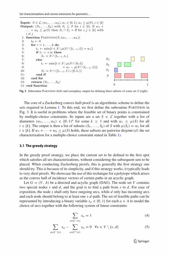
Fig. 3 Subroutine Partition (left) and exemplary output for defining three subsets of some set S (right)

The core of a Zuckerberg convex-hull proof is an algorithmic scheme to define thesets required in Lemma 1. To this end, we first define the subroutine Partition inFig. 3. It is useful in problems where the feasible set of binary points is constrainedby multiple-choice constraints. Its inputs are a set S ∈ L together with a list ofdiameters (w1, . . . , wk) ∈ [0, 1)n for some k ≥ 1 and with wi ≤ μ(S) for alli ∈ [k]. The output is then a list of subsets (S1, . . . , Sk) of S with μ(Si ) = wi for alli ∈ [k]. If w1 + · · · + wk ≤ μ(S) holds, these subsets are pairwise disjoint (cf. the setcharacterization for a multiple-choice constraint stated in Table 1).

3.1 The greedy strategy

In the greedy proof strategy, we place the current set to be defined to the first spotwhich satisfies all set characterizations, without considering the subsequent sets to beplaced. When conducting Zuckerberg proofs, this is generally the first strategy oneshould try. This is because of its simplicity, and if this strategy works, it typically leadsto very short proofs.We showcase the use of this technique for a polytope which arisesas the convex hull of incidence vectors of certain paths in an acyclic graph.

Let G = (V , A) be a directed and acyclic graph (DAG). The node set V containstwo special nodes s and d, and the goal is to find a path from s to d. For ease ofexposition, the node s shall only have outgoing arcs, while d only has incoming arcsand each node should belong to at least one s-d-path. The set of feasible paths can berepresented by introducing a binary variable xa ∈ {0, 1} for each a ∈ A to model thechoice of arcs together with the following system of linear constraints:

∑a∈δ−(s)

xa = 1 (4)

∑a∈δ−(v)

xa −∑

a∈δ+(v)

xa = 0 ∀v ∈ V \ {s, d} (5)

123


∑a∈δ+(d)

xa = 1 (6)

0 ≤ xa ≤ 1. (7)

We now give a Zuckerberg-type proof for the well-known result stating the inte-grality of the above system.

Theorem 3 Let P := conv{x ∈ {0, 1}|A| | (4) to (7)} be the s-d-path-polytope andH := {x ∈ [0, 1]|A| | (4) to (7)} its linear relaxation. Then we have P = H.

Proof It is obvious that P ⊆ H . In order to prove H ⊆ P , we need to transform theconstraints (4) to (6) into set characterizations. Referring to Table 1, we can directlystate them as follows:

|{i ∈ δ−(s) | t ∈ Si }| = 1 ∀t ∈ U , (8)

|{i ∈ δ−(v) | t ∈ Si }| = |{ j ∈ δ+(v) | t ∈ S j }| ∀v ∈ V \ {s, d},∀t ∈ U , (9)

|{i ∈ δ+(d) | t ∈ Si }| = 1 ∀t ∈ U . (10)

Note that inequalities (7) do not have a set characterization of their own above asthey are already implied by the fact that all sets need to be subsets of U = [0, 1).Further, inequality (6) is redundant and only stated for better readability. Therefore,set characterization (10) is already implied by (8) and (9).

For each point h ∈ H , we now need to find sets Sa for all a ∈ A such thatμ(Sa) = ha as well as set characterizations (8) to (10) hold. The sets Sa are defined viathe routine Define-s-d-Path-Subsets presented in Fig. 4. The algorithm processesthe nodes in the graph in topological order, where TopologicalSort is any routineproducing such an order. In each iteration, it places the sets for all outgoing arcs ofthe current node via a call to the routine Partition. This ensures that conditions (8)to (10) are satisfied. By starting at node s and processing the nodes in topologicalorder, we are sure that once a node is reached all sets for the incoming arcs have beendefined. Finally, the make-up of subroutine Partition guarantees μ(Sa) = ha for alla ∈ A. Thus, we have proved H ⊆ P . ��

The greedy proof technique is most promising if the problem at hand only featureslocal constraints (like flow conservation or variable bounds) as they allow to placethe sets in consecutive fashion. Constraints inducing global couplings between thevariables make it harder to use. In the online supplement [7], we give further examplesfor the use of this technique in the context of clique and stable-set problems. A naturalfurther question is whether the proof can be extended to general graphs instead ofacyclic ones. The vertices are then not only paths, but rather combinations of pathsand cycles. For the placement of the sets Si , we need to assign cycles to paths, forwhich there are many different options, and there is no clear order in which to processthe sets to obtain a feasible solution.

123


Fig. 4 RoutineDefine-s-d-Subsets (top), exemplary graph with 6 nodes (bottom left) and possible outputof the routine for the point h = (0.8, 0.1, 0.1, 0.6, 0.3, 0.4, 0.3, 0.2) (bottom right). There are four paths inthe graph, namely (a1, a2, a3), (a8, a4), (a1, a7, a5) and (a1, a6, a4). Those parts of the sets correspondingto a certain path are marked in the same colour (colour figure online)

3.2 Zuckerberg proofs via feasibility subproblems

A further strategy for Zuckerberg proofs is to place groups of related sets simultane-ously. If the correct placement of these sets is too difficult to be stated explicitly, itcan be worthwhile to define an auxiliary optimization problem from whose solution afeasible placement of the sets can be extracted. It is then necessary to prove that thissubproblem is feasible for each point h ∈ H to be tested. In case the optimizationproblem is a linear program, one can try to use the Farkas lemma for the feasibilityproof. We highlight this technique at the hand of a polynomial-time solvable specialcase of the clique problem with multiple-choice constraints.

Let G = (V , E) be an m-partite graph for some m ≥ 1, and let V = {V1, . . . , Vm}be the corresponding partition of the node set V . The clique problem with multiple-choice constraints (CMPC) asks to find a clique of cardinality m in G. While it isNP-complete in general to decide if such a clique exists (see [5]), there are severalrelevant special cases where this is possible in polynomial time. These include CPMCunder staircase compatibility [3,4] and CPMC under a cycle-free dependency graph[5]. The referenced works give complete convex-hull descriptions for these two cases.

123


The CPMC polytope is the convex hull of all incidence vectors of m-cliques in G.In the online supplement [7], we will reprove the result from [3] that staircase compat-ibility allows for totally unimodular formulations of polynomial size for the CPMCpolytope. Here we consider the case where there are no cyclic dependencies betweenthe subsets Vi . The authors of [5] give a complete convex-hull description for thiscase whose correctness they prove via the alternating colouration theorem (see [13]).Alternatively, they hint a proof via the strong perfect-graph theorem (see [8]). Bothapproaches lead to the result that the graphG is perfect.As theCPMCpolytope is a faceof the ordinary clique polytope on G, this readily yields a complete description of itsconvex hull. In the following, we will give a much more elementary convex-hull proofbased on Zuckerberg’s method which does neither use alternating colourations norperfectness. In addition, we will be able to state the vertices spanning any given pointin the CPMC polytope, for which there is no obvious derivation using the approachespresented in [5].

Let G := (V, E) with

E := {{Vi , Vj } ⊆ V | (∃u ∈ Vi )(∃v ∈ Vj ) {u, v} /∈ E}

denote the dependency graph of G. Let Gi j = (Vi j , Ei j ) be the subgraph inducedby Vi ∪ Vj . Note that {Vi , Vj } ∈ E is equivalent to the subgraph Gi j not being acomplete bipartite graph. For ease of notation, we further define the neighbourhoodN j (U ) ⊆ Vj of a subset U ⊆ V in Vj as

N j (U ) := {v ∈ Vj | (∃u ∈ U ) {u, v} ∈ E}.

It represents those nodes in Vj for which there is a compatible node in U .We will now show that the CPMC polytope is completely described via the stable-

set constraints and the trivial constraints if the dependency graph is a forest.

Theorem 4 [5, Theorem 3.1] Let

P(G,V) := conv

⎧⎪⎨⎪⎩ x ∈ {0, 1}|E |

∣∣∣∣∑v∈Vi

xv = 1 ∀Vi ∈ V

xi + x j ≤ 1 ∀{i, j} /∈ E

⎫⎪⎬⎪⎭

be the CPMC polytope and

H(G,V) := conv

⎧⎪⎪⎪⎨⎪⎪⎪⎩

x ∈ [0, 1]|E |∣∣∣∣

∑v∈Vi

xv = 1 ∀Vi ∈ V∑v∈C

xv ≤ 1 ∀ stable sets C ⊆ V

⎫⎪⎪⎪⎬⎪⎪⎪⎭

its stable-set relaxation. If G has no cycles, we have P(G,V) = H(G,V).

123


Fig. 5 Routine Define-CMPCF-Sets

Proof The inclusion P(G,V) ⊆ H(G,V) holds trivially. We now show the reverseinclusion. The procedure to define the sets Si for i ∈ V is given via the two routinesDefine-CMPCF-Subsets and Traverse-Tree in Fig. 5.

The former routine iterates over all connected components in the dependencygraph G, which are trees in our case. In Line 3, it selects an arbitrary node (sub-set in the partition) Vi as the root node of the current tree. Then it fixes an arbitraryordering of the elements v ∈ Vi and places the corresponding sets next to each othervia a call to subroutine Partition in Line 5. Finally, it traverses the tree recursivelyin Lines 6–8 by calling the routine Traverse-Tree, whose input is a subset Vi forwhich all sets have already been defined, together with a set Vj , which is a neighbourof Vi . The routine then places all sets for Vj . To do so, it solves a linear feasibilityproblem in Line 12 which is defined as follows: the variables xi j ∈ R+ encode themeasure of the overlap between the sets Si and S j . These overlaps need to fulfil theset characterizations

|{v ∈ Vi | t ∈ Sv}| = 1 ∀Vi ∈ V,∀t ∈ U , (11)

|{v ∈ C | t ∈ Sv}| ≤ 1 ∀ stable sets C ⊆ V ,∀t ∈ U , (12)

123


which leads to the following linear programming system:

∑j∈N (i)

xi j = hi ∀i ∈ Vi , (13a)

∑i∈N ( j)

xi j = h j ∀ j ∈ Vj , (13b)

xi j ≥ 0 ∀(i, j) ∈ Ei j . (13c)

In Lines 13–22, the routine chooses the sets for all elements in Vj accordingly. Itthen proceeds recursively in Lines 23–25.

It remains to show that problem Eq. (13) is feasible for all h ∈ H . To prove this,we analyse its dual Farkas system, which is given by

∑i∈Vi

hi yi +∑j∈Vj

h j y j < 0, (14a)

yi + y j ≥ 0 ∀(i, j) ∈ Ei j . (14b)

We will prove by contradiction that Eq. (14) has no solution in order to show thefeasibility of Eq. (13). To this end, consider some point h ∈ H and let y be a corre-sponding solution of Eq. (14). We first argue that we can assume y ∈ {−1, 0, 1}|Vi j |w.l.o.g. Via rescaling, we can assume that the lowest entry of y is −1. Now letW := {k ∈ Vi j | yk < 0}.We can assume yk = 0 for all elements in Vi j \(W ∪N (W )),since this is always feasible if yk > 0 was feasible. Further, let P := (p1, . . . , pq) be asorted list of the elements in {yk ∈ R | k ∈ W } in decreasing order with q := |P|. Forp ∈ P , let Q p := {k ∈ W | yk = p}, and let R := N (Q p1)\ N (Q p2)∪· · ·∪ N (Q pq ).Then check if

∑v∈R hv yv + ∑

v∈Q p1hv yv ≥ 0 holds. If yes, set yk = 0 for

k ∈ Q p1 ∪ R. If no, set yk = p2 for k ∈ Q p1 and yk = −p2 for k ∈ R. Nowupdate W and let P := (p1, . . . , pq−1) again be a sorted list of the elements in{yk ∈ R | k ∈ W } in decreasing order. This procedure lets P now contain preciselyone element less than before. Repeat this until there is only one element in P left,which has to be −1, so we can set yk = 1 for all k ∈ N (W ). This way, we have foundan integral solution to Eq. (14). We then have

∑k∈N (W )

hk yk +∑k∈W

hk yk < 0,

∑k∈N (W )

hk −∑k∈W

hk < 0,

1 −∑

k∈Vi j \N (W )

hk −∑k∈W

hk < 0,

∑k∈Vi j \N (W )

hk +∑k∈W

hk > 1.

123


However, this is impossible, since the nodes (Vi j \ N (W )) ∪ W form a stable set,which leads to a contradiction. ��

Via Corollary 1, this directly allows us to represent a point h ∈ H as a convexcombination of the vertices of the CMPC polytope, which extends the results from[5].

This technique could be generalized by passing from linear to more complex auxil-iary problems to determine the placement of the sets. The core of this proof techniqueconsists in analysing the auxiliary problem to verify its feasibility for any inputs arisingwithin the algorithmic scheme.

3.3 The transformation strategy

The third proof strategy we present makes use of the fact that it can be easier to placethe sets for some points within a given polytope than for others. Thus, it is sometimeshelpful to transform the arbitrary point to be tested for membership in Lemma 1 toanother, auxiliary point first. Then, after placing the sets for this auxiliary point, theyare retransformed to represent the original point. Such a transformation must respectthe set characterizations of the vertex set. We present this technique exemplarily forthe convex hull of all incidence vectors of stable sets in a single odd cycle.

The stable-set polytope of a graph G = (V , E) is defined as the convex hull of allvectors x ∈ {0, 1}|V | that satisfy the edge constraints

xi + x j ≤ 1 ∀(i, j) ∈ E . (15)

If G is a cycle, the odd-cycle inequality

∑i∈V

xi ≤ |V | − 1

2(16)

is valid for the corresponding stable-set polytope. For an odd-cycle, it is sufficientto describe the complete convex hull, together with inequalities (15) and the trivialinequalities.

Theorem 5 Let G = (V , E) be an odd hole, let P(G) := {x ∈ {0, 1}|V | |(15) and (16)} be the stable-set polytope on G, and let H(G) := {x ∈ [0, 1]|V | |(15) and (16)} be its linear relaxation. Then we have P = H.

Proof It is obvious that P(G) ⊆ H(G). For the converse, consider the set characteri-zations of (15) and (16), which are given by:

Si ∩ S j = ∅ ∀(i, j) ∈ E, (17)

|{i ∈ B | t ∈ Si }| ≤ |V | − 1

2∀t ∈ U (18)

(cf. Table 1). For a given point h ∈ H(G), we then need to find sets Sv for each v ∈ Vsuch that μ(Sv) = hv and the above conditions hold. We define these sets in routine

123


Fig. 6 Routine Define-odd-cycle-Stable-Set-Subsets (top), exemplary graph with five nodes (bottomleft) and possible output of the routine for the point given by h = (0.5, 0.2, 0.3, 0.1, 0.1). It is blown upto h = (0.8, 0.2, 0.8, 0.1, 0.1). The point h can be written as a convex combination of incidence vectorsbelonging to five stable sets, namely {u1, u3}, {u1}, ∅, {u2, u4} and {u2, u5}, each non-empty one markedwith same colour (bottom right) (colour figure online)

Define-Odd-Cycle-Stable-Sets-Subsets, given in Fig. 6. First, in Line 2/3, we fixan ordering of the nodes which respects the order of the cycle. In Lines 4–8, the point his then shifted to a point h on the boundary of H(G) by increasing h componentwiseuntil in each iteration at least one of the inequalities (15) and (16) becomes active.By induction, for the resulting point h the inequality h ≥ h holds component-wiseand we have

∑|V |i=1 hi = (|V | − 1)/2. Now, auxiliary sets Sv , v ∈ V , are placed

in consecutive order along the cycle in Line 9, based on the diameters stored in h.Observe that, in particular, the first set is defined as Sv1 = [0, hv1) and the last one asSv|V | = [1 − hv|V | , 1), thus they satisfy set characterizations (17) and (18). Finally, inLines 10–12, the diameters of the auxiliary sets are reduced such that they correspondto the components of h to obtain the final sets Sv , v ∈ V . It is obvious that these setssatisfy μ(Sv) = hv for all v ∈ V , and the reduction does not invalidate any of the setcharacterizations (17) or (18). Therefore, we have proved H(G) ⊆ P(G). ��

In the above proof, an auxiliary point h ∈ H is constructed by greedily increasingthe coordinates of the point h to be tested. The sets for h are then placed next toeach other, modulo 1 (the diameter of U ). The backward transformation then simplyshrinks the sets to fit the size of the original coordinates of h while maintaining thevalidity of all set characterizations. As shown in Fig. 6, the final sets after backward

123


transformation are not always placed next to each other due to the gaps arising fromthe shrinking step. A direct placement of these sets for the original point seems tomore involved, since it is not obvious how to calculate the gaps between adjacent setsa priori.

It is a natural consideration to extend the proofs of Theorems 4 and 5 to moregeneral graphs. For example, it might be possible to use Zuckerberg’s method to showthat the convex hull of the clique polytope on a perfect graph is given by the stable-setconstraints and the non-negativity constraints. This would directly imply Theorems 4after showing that the graph G is perfect under the stated assumption. Similarly,using Zuckerberg’s method to show that the stable-set polytope on a series-parallelgraph is given by the edge constraints, the odd-hole constraints and the non-negativityconstraints would reprove the according result from [17] and easily imply Theorem 5.However, both seem not straightforward to do, as one would first need to find a naturalorder along which to process each variable for placing the corresponding sets Si . Asuitable decomposition approach based on graph structure is usually beneficial here.For example, in the case of series-parallel graphs, an ear-decomposition of the graphseems to be a good starting point. This could be an interesting topic for future research.

4 Extensions of Zuckerberg’s method for general convex sets

Both the original proof technique by Zuckerberg from [22] and its simplification in[11] are applicable to 0/1-polytopes only. In the following, we will derive extensionsof Zuckerberg’s method which enable us to conduct geometric convex-hull proofsfor arbitrary convex sets. This includes, in particular, general integer polyhedra. Theunderlying idea is to pass from intervals in U = [0, 1) to rectangles in R2 whenconstructing the sets to represent a given point h in some convex set H . Recall thatthe original method interprets each of these dimension-many sets as either a 0- ora 1-coordinate of a vertex in a 0/1-polytope; a coordinate of the vertex which belongsto some t ∈ U is 1 if the corresponding set includes t , and 0 otherwise. The verticesassociated with the sets representing a point h in the polytope define a convex combi-nation spanning h. Our extension of Zuckerberg’s method gives the intervals makingup these sets a height to encode the coordinates of arbitrary points in H instead of only0/1-points. This idea will lead to generalized versions of the theorems in Sect. 2 whichcan be used to prove the completeness of convex-hull representations for general con-vex sets. Furthermore, they also allow to compute convex combinations spanning acertain h ∈ H using any points in H , not necessarily extreme points.

To formalize the new approach, we first define the set

RQ :={

([a, b), c) ∈ P(Q) × R

∣∣∣∣ a < b, c = 0

},

where Q is chosen as either U = [0, 1) or as R+. The set Q specifies therange of coefficients which are allowed in a linear combination representing someh ∈ H . We use Q = U to construct convex combinations and Q = R+ for coniccombinations. We interpret RQ as the set of all non-degenerate, axis-parallel rectan-

123


gles R = ([a, b), c) ∈ R2, which are uniquely defined by stating the two diagonallyopposite vertices (a, 0) and (b, c). The sign of c indicates if a rectangle points into theupper half-space (c > 0) or the lower half-space (c < 0). Let q(R) := (b − a)c andz(R) := c denote the signed area and the signed height of the rectangle R respectively.Further, let y : Q×RQ → {0, 1} be an indicator function defined as follows. For somet ∈ Q and R = ([a, b), c) ∈ RQ it is y(t, R) = 1 if a ≤ t ≤ b, and y(t, R) = 0otherwise. In other words, y indicates whether t belongs to the support of R, in whichcase we call R active at t . We call two rectangles R1 and R2 non-overlapping if thereexists no t ∈ Q such that both y(t, R1) = 1 and y(t, R2) = 1 hold.

In a similar fashion as in Sect. 2, we then define LQ as the set of all unions of finitelymany non-degenerate, non-overlapping rectangles fromRQ and μQ as the Lebesguemeasure restricted to LQ , that is

LQ :={

{R1, . . . , Rk}∣∣∣∣ k ∈ N ∧ R1, . . . , Rk ∈ RQ∧

Ri and R j are non-overlapping ∀i, j ∈ [k], i = j

}

μQ(S) :=k∑

i=1

q(Ri ) for any S = {R1, . . . , Rk} ∈ LQ .

Moreover, we define the indicator function φQ : Q × LQ → R,

φQ(t, S) :={

z(R) if y(t, R) = 1 for any R ∈ {R1, . . . , Rk},0 otherwise,

where S is uniquely represented as S = {R1, . . . , Rk} for some k ∈ N in Ri ∈ RQ ,i ∈ [k]. It returns the height of the rectangle which is active at t ∈ Q if there isone. Note that the active rectangle is unique in this case as the Ri forming S arenon-overlapping. Finally, let ϕQ : Q × (LQ)n → Rn, ϕQ(t, S1, . . . , Sn) = v, wherevi := φQ(t, Si ) for i ∈ [n]. Here we interpret the heights of the rectangles which areactive at t as the coordinates of a vector inRn .

With the above definitions, we are equipped to state our extensions of Zuckerberg’smethod. As a useful shorthand notation used in the proofs, we define the union S1∪ S2of two sets S1, S2 ∈ LQ as the unique S ∈ LQ such that for all t ∈ Q we haveφQ(t, S) = φQ(t, S1)+φQ(t, S2). Informally speaking, thismeanswe add the heightsof the rectangles which are active at a certain t to form the union S.

We start with an extension which enables us to conduct geometric convex-hullproofs for general convex sets.

Theorem 6 (Zuckerberg’s method for general convex sets) Let F ⊆ Rn and h ∈ Rn.Then we have h ∈ conv(F) iff there are sets S1, . . . , Sn ∈ LU such that μU (Si ) = hi

for all i ∈ [n] and ϕU (t, S1, . . . , Sn) ∈ conv(F) for every t ∈ U.

Proof If h ∈ conv(F), then there exist ξ1, . . . , ξ r ∈ conv(F), for some r ∈ N+, suchthat h can be written as h = λ1ξ

1 +· · ·+λrξr with λ1 +· · ·+λr = 1 and λk ≥ 0 for

all k ∈ [r ]. We can then define a partition U = I1 ∪ · · · ∪ Ir by setting I1 := [0, λ1)

123


and Ik := [λ1 + · · · + λk−1, λ1 + · · · + λk) for k ∈ {2, . . . , r}. This allows us to set

Si :=⋃

k∈[r ]: ξ ki =0

(Ik, ξki ) ∈ LU , i ∈ [n],

with rectangles (Ik, ξki ) ∈ RU . For all i ∈ [n], we can conclude

μU (Si ) =∑

k∈[r ]: ξ ki =0

μU ((Ik, ξki )) =

∑k∈[r ]: ξ k

i =0

λkξki =

∑k∈[r ]

λkξki = hi .

Furthermore, for every t ∈ U there is a unique index k with t ∈ Ik , and thus wehave

ϕU (t, S1, . . . , Sn) = ξ k ∈ conv(F).

Conversely, if the Si are sets with the described properties, let ξ1, . . . , ξ r be anordering of the elements in

{ξ ∈ conv(F)

∣∣∣∣ ϕU (t, S1, . . . , Sn) = ξ for some t ∈ U

}.

The above set is finite, since each Si is a finite union of rectangles. We can set, byslight abuse of notation,

λk := μU({

(t, 1) ∈ U × {1}∣∣∣∣ ϕU (t, S1, . . . , Sn) = ξ k

})

for k ∈ [r ] to obtain the required convex representation h = λ1ξ1 + · · · + λrξ

r . Tosee this, we can easily verify

Si =⋃

k∈[r ]: ξ ki =0

{(t, ξ k

i ) ∈ U × R

∣∣∣∣ ϕU (t, S1, . . . , Sn) = ξ k}

for all i ∈ [n]. We then conclude for all i ∈ [n]:∑k∈[r ]

λkξki =

∑k∈[r ]

μU({

(t, 1) ∈ U × {1}∣∣∣∣ ϕU (t, S1, . . . , Sn) = ξ k

})ξ k

i

=∑

k∈[r ]: ξ ki =0

μU({

(t, ξ ki ) ∈ U × R

∣∣∣∣ ϕU (t, S1, . . . , Sn) = ξ k})

= μU

⎛⎜⎝ ⋃

k∈[r ]: ξ ki =0

{(t, ξ k

i ) ∈ U × R

∣∣∣∣ ϕU (t, S1, . . . , Sn) = ξ k}⎞⎟⎠

123


= μU (Si ) = hi .

��Note that in the first line of the proof, h does not necessarily have to be a convex

combination of points in F , but we can also make use of points in conv(F). This isby intention in order to allow for more freedom in conducting convex-hull proofs.In Sect. 4.1 we will give a corresponding example in which we express h as integerpoints (not vertices) inside F .

Theorem 6 generalizes Theorem 1 in twoways. Themethod nowworks for arbitraryconvex sets, instead of only 0/1-polytopes. Note that Zuckerberg’s original methodcan be recovered by discarding the height of the rectangles and only checking whethera given set is active at some t ∈ U . We also remark that in Theorem 6 we can nowwrite the point h as a linear combination of points in conv(F), not only points in F .This allows an additional degree of freedom for convex-hull proofs which Theorem 1does not offer.

Using our extended framework, we can also determine a representation of any givenpoint h ∈ H as a convex combination of points in F if we find corresponding setsS1, . . . , Sn fulfilling the requirements of Theorem 6. To state this result, we define thetwo sets

F(S1, . . . , Sn) :={

ξ ∈ conv(F)


}

and, for each ξ ∈ Rn ,

LUξ (S1, . . . , Sn) :=

{t ∈ U

∣∣∣∣ ϕU (t, S1, . . . , Sn) = ξ

}.

The following corollary then directly follows from the proof of Theorem 6.

Corollary 2 (Convex combinations for general convex sets) Under the same assump-tions as in Theorem 6, let λξ := μU (LU

ξ (S1, . . . , Sn)) for each ξ ∈ F(S1, . . . , Sn).Then we have h = ∑

ξ∈F(S1,...,Sn) λξ ξ ,∑

ξ∈F λξ = 1 and λξ ≥ 0 for all

ξ ∈ F(S1, . . . , Sn).

The definition of a set characterization (Definition 1) can now be restated in a moregeneral form as well.

Definition 2 (Set characterization of a constraint) Let f : F → R, let b ∈ R, andlet S1, . . . Sn ∈ LU . The set characterization of some constraint f (x) ≤ b is thefollowing logic statement:

f (φU (t, S1), . . . , φU (t, Sn)) ≤ b holds for all t ∈ U .

Similar to before, we can use this concept to facilitate finding sets Si which char-acterize a point h ∈ H according to Theorem 6.

123


Lemma 2 Let F := {x ∈ Zn | f j (x) ≤ b j ∀ j ∈ [m]} for some m ∈ N. Further, letP := conv(F), and let H ⊆ Rn be some convex set. We have H = P iff both F ⊆ Hholds and for each h ∈ H there are sets S1, . . . , Sn ∈ LU with μU (Si ) = hi for alli ∈ [n] which satisfy the set characterization for each constraint f j (x) ≤ b j , j ∈ [m]and φU (t, Si ) ∈ Z for all i ∈ [n], t ∈ U.

Polyhedra, which are special convex sets, can be written as a convex combinationof a finite sets of points plus a conic combination of a finite set of rays In the following,we give an alternative version of Theorem 6 for polyhedra making use of this fact.

Theorem 7 (Zuckerberg’s method for polyhedra) LetF ⊆ Rn and E ⊆ Rn be a finite,non-empty set of points, h ∈ Rn. Then we have h ∈ conv(F) + cone(E) iff there aresets S1, . . . , Sn ∈ LU and sets S′

1, . . . , S′n ∈ LR+ such that μU (Si ) + μR+(S′

i ) = hi

for all i ∈ [n], ϕU (t, S1, . . . , Sn) ∈ conv(F) for all t ∈ U and ϕR+(t ′, S′1, . . . , S′

n) ∈cone(E) for all t ′ ∈ R+.

Proof If h ∈ conv(F) + cone(E), then there exist ξ1, . . . , ξ r ∈ conv(F) for somer ∈ N+ and ζ 1, . . . , ζ q ∈ cone(E) for some q ∈ N+ such that h can be written ash = λ1ξ

1 + · · · + λrξr + η1ζ

1 + · · · + ηqζ q with λ1 + · · · + λr = 1, λk ≥ 0 for allk ∈ [r ] and ηk ≥ 0 for all k ∈ [q]. Define now the partition U = I1 ∪ · · · ∪ Ir bysetting I1 := [0, λ1) and Ik := [

λ1 + · · · + λk−1, λ1 + · · · + λk) for k ∈ {2, . . . , r}.In addition, we define I1 := [0, η1) and Ik := [

η1 + · · · + ηk−1, η1 + · · · + ηk) fork ∈ {2, . . . , q}. With

Si :=⋃

k∈[r ]: ξ ki =0

(Ik, ξki ), S′

i :=⋃

k∈[q]: ζ ki =0

( Ik, ζki )

for i ∈ [n], we find

μU (Si ) + μR+(S′i ) =

∑k∈[r ]: ξ k

i =0

μU ((Ik, ξki )) +

∑k∈[q]: ξ k

i =0

μR+(( Ik, ζki ))

=∑

k∈[r ]: ξ ki =0

λkξki +

∑k∈[q]: ζ k

i =0

ηkζki =

∑k∈[r ]

λkξki +

∑k∈[q]

ηkζki

= hi .

Moreover, for each t ∈ U , there is a unique index k with t ∈ Ik , and thus

ϕU (t, S1, . . . , Sn) = ξ k ∈ conv(F).

Similarly, for each t ∈ R+, there is either a unique index k with t ∈ Ik , or there isno such index. Thus, we conclude

ϕR+(t, S′1, . . . , S′

n) = ζ ∈ cone(E).

Especially, if there is no index k as outline above, we have ζ = 0.

123


Conversely, if Si and S′i are sets with the stated properties, let ξ1, . . . ξ r be an

ordering of the elements in

{ξ ∈ conv(F)


},

and let ζ1, . . . ζq be an ordering of the elements in

{ζ ∈ cone(E)

∣∣∣∣ ϕR+(t, S′1, . . . , S′

n) = ζ for some t ∈ R+}

.

Both sets are finite, since all Si and S′i are finite unions of rectangles. For k ∈ [r ]

and p ∈ [q], we can set

λk := μU({

(t, 1) ∈ U × {1}∣∣∣∣ ϕU (t, S1, . . . , Sn) = ξ k

}),

ηp := μR+({

(t, 1) ∈ R+ × {1}∣∣∣∣ ϕR+(t, S′

1, . . . , S′n) = ζ p

})

to obtain the required convex representation h = λ1ξ1+· · ·+λrξ

r +η1ζ1+· · ·+ηqζ q .

To this end, observe that for all i ∈ [n] we have

Si =⋃

k∈[r ]: ξ ki =0

{(t, ξ k

i ) ∈ U × R

∣∣∣∣ ϕU (t, S1, . . . , Sn) = ξ k}

,

S′i =

⋃k∈[q]: ζ k

i =0

{(t, ξ k

i ) ∈ R+ × R

∣∣∣∣ ϕR+(t, S′1, . . . , S′

n) = ζ k}

.

For all i ∈ [n], this leads to∑k∈[r ]

λkξki =

∑k∈[r ]

μU({

(t, 1) ∈ U × {1}∣∣∣∣ ϕU (t, S1, . . . , Sn) = ξ k

})ξ k

i

=∑

k∈[r ]: ξ ki =0

μU({

(t, ξ ki ) ∈ U × R

∣∣∣∣ ϕU (t, S1, . . . , Sn) = ξ k})

= μU

⎛⎜⎝ ⋃

k∈[r ]: ξ ki =0

{(t, ξ k

i ) ∈ U × R

∣∣∣∣ ϕU (t, S1, . . . , Sn) = ξ k}⎞⎟⎠

= μU (Si )

and

123


∑k∈[q]

ηkζki =

∑k∈[q]

μR+({

(t, 1) ∈ R+ × {1}∣∣∣∣ ϕR+(t, S′

1, . . . , S′n) = ζ k

})ζ k

i

=∑

k∈[q]: ζ ki =0

μR+({

(t, ζ ki ) ∈ R+ × R

∣∣∣∣ ϕR+(t, S′1, . . . , S′

n) = ζ k})

= μR+

⎛⎜⎝ ⋃

k∈[p]: ζ ki =0

{(t, ζ k

i ) ∈ R+ × R

∣∣∣∣ ϕR+(t, S′1, . . . , S′

n) = ζ k}⎞⎟⎠

= μR+(S′i ).

This yields

r∑k=1

λkξki +

q∑k=1

ηkζki = μU (Si ) + μR+(S′

i ) = hi .

��When we conduct a convex-hull proof via Theorem 6, we implicitly write the given

point h as a convex combination of other points in H (most often extreme points). Incontrast, Theorem 7 allows us to express h as both a convex and conic combinationof points spanning H . This is especially interesting for polyhedra, which can be splitinto a convex and a conic part. Both versions are valuable tools and allow for differentproof strategies as the example in Sect. 4.2 shows.

If we succeed in giving a convex-hull via Theorem 7, we can again deduce convexand conic combinations afterwards.

Corollary 3 (Convex combinations for polyhedra) Under the same assumptions asin Theorem 7, let λξ := μU (LU

ξ (S1, . . . , Sn)) for all ξ ∈ F and ηζ :=μR+(LR+

ζ (S′1, . . . , S′

n)) for all ζ ∈ E . Then we have h = ∑ξ∈F λξ ξ + ∑

ζ∈E ηζ ζ ,∑ξ∈F λξ = 1 with λξ ≥ 0 for all ξ ∈ F and ηζ ≥ 0 for all ζ ∈ E .

It is straightforward to adjust the definition of set characterizations fromDefinition 2to include the conic part as well. We will, however, skip this for reasons of space.

To define the sets in a convex-hull proof according to Theorems 6 or 7, it will behelpful to introduce the auxiliary function o : Q × U → L × U ,

o(t, a) :={

([t, t + a), t + a) if t + a ≤ 1,

([t, 1) ∪ [0, t + a − 1), t + a − 1) otherwise.

This function determines an interval starting at t ∈ Q and of diameter a ∈ U ,modulo 1. It returns an ordered pair consisting of the interval and its end point, whichwill be useful when placing rectangles adjacent to each other.

Wewill now give some indicative first examples to illustrate how the results derivedin this section can be used to give convex-hull proofs.

123


Fig. 7 Routines Define-Simplex-Subsets-A (top left) and Define-Simplex-Subsets-B (bottom left),exemplary constructions for the 3-dimensional simplex H with right-hand side b = 4 for the point hwith (h1, h2, h3) = (1, 1.5, 0.8) for Define-Box-Subsets-A (top right) and Define-Box-Subsets-B(bottom right). Via Define-Box-Subsets-A, we obtain h = 0.25(4, 0, 0)+0.375(0, 4, 0)+0.2(0, 0, 4)+0.175(0, 0, 0) while Define-Box-Subsets-B yields h = 0.3(1, 2, 1) + 0.2(1, 2, 0) + 0.5(1, 1, 1). Thoseparts of the sets which belong to the same vertex are marked with the same colour; the numbers representthe height of each rectangle, i.e. the coordinates of the vertices (colour figure online)

4.1 Convex-hull proofs using interior points

We start with the example of a simplex to show that the point h ∈ H does notnecessarily have to be written as a convex combination of vertices, but that it is alsopossible to characterize it via sets corresponding to other points in the interior. LetF := {x ∈ Zn | ∑n

i=1 xi ≤ b, x ≥ 0} and H := {x ∈ Rn | ∑ni=1 xi ≤ b, x ≥ 0}

with some b ∈ N. The set characterizations for the simplex constraint and the non-negativity constraint can be stated as

n∑i=1

φU (t, Si ) ≤ b ∀t ∈ U , (19)

φU (t, Si ) ≥ 0 ∀i ∈ [n], ∀t ∈ U (20)

respectively. A possible construction of the sets Si for Theorem 7 is given in routineDefine-Simplex-Subsets-A, and a different variant is given in routine Define-Simplex-Subsets-B, both stated in Fig. 7. Via the first variant, the point h ∈ His always written as a convex combination of vertices of H , while in the second onethe point may also be represented using integral points inside the polytope. By con-struction, both routines return sets Si with μU (Si ) = hi for all i ∈ [n]. The inequalitiesdefining H ensure that the combined width of the rectangles fits into U , and thus therequirements of Theorem 7 are fulfilled in both cases. This yields two different proofsfor H = conv(F) and shows the additional flexibility Theorem 7 offers.

123


Fig. 8 Routine Define-Simplex+Cone-Subsets (top), exemplary construction for the 3-dimensionalpolyhedron H with right-hand side b = 1 for the point h with (h1, h2, h3) = (1, 1.5, 0.8) for Define-Conv-Cone-Subsets (bottom). The latter decomposes h into h = g + v, where g ≈ 0.3(1, 0, 0) +0.45(0, 1, 0) + 0.24(0, 0, 1) and v ≈ 0.7(1, 0, 0) + 1.05(0, 1, 0) + 0.56(0, 0, 1). The vector g is repre-sented by a convex combination of the vertices of the polytopal part of H , and v as a conic combination ofits rays. Those parts of the sets which belong to the same vertex or ray are marked with the same colour;the numbers represent their coordinates (colour figure online)

4.2 Convex-hull proofs for unbounded polyhedra

We continue with a modification of the previous simplex example, where we demon-strate the difference it makes to apply either Theorems 6 or 7 when showing integralityof an unbounded polyhedron. Let F := {x ∈ Zn | ∑n

i=1 xi ≥ b, x ≥ 0} andH := {x ∈ Rn | ∑n

i=1 xi ≥ b, x ≥ 0} with some b ∈ N. The set characterizationsfor the two constraints defining F and H can be stated as

n∑i=1

φU (t, Si ) ≥ b ∀t ∈ U , (21)

φU (t, Si ) ≥ 0 ∀i ∈ [n], ∀t ∈ U . (22)

We can reuse routine Define-Simplex-Subsets-B from Fig. 7 to construct ade-quate sets Si for Theorem 6, which proves the equivalence of conv(F) and H . Analternative representation ofF is given byF = b conv(e1, . . . , en)+cone(e1, . . . , en).Using the construction provided by routine Define-Conv-Cone-Subsets in Fig. 8,we can invoke Theorem 7 and thus prove H = conv(F) in an alternative fashion.We can use both methods in order to prove the same statement. However, we obtaindifferent linear combinations representing a given point h. Theorem 6 gives us a con-vex combination of arbitrary points in H . In contrast, Theorem 7 returns two sets ofpoints, vertices and rays, such that a convex combination of the vertices plus a coniccombination of the rays yields h. Depending on the problem at hand, both strategiesmight be the one which is best suited for a convex-hull proof.

123


Fig. 9 Routine Define-Ball-Subsets (left), exemplary construction for the point h with (h1, h2) =(1.1, 1.9) (right). The routine returns the representation h ≈ 0.39(0.56, 1.9) + 0.61(1.44, 1.9). The figureinside a rectangle indicates its height

4.3 Convex-hull proofs for non-linear convex sets

Finally, we show that our new criteria for convex-hull proofs can also be used withnon-polyhedral convex sets. To do so, we use the example of the unit-ball in R2. LetF := {x ∈ R2 | (x1−1)2+(x2−1)2 = 1} and H := {x ∈ R2 | (x1−1)2+(x2−1)2 ≤1}. The set characterization for the quadratic constraint defining F is given by

(φU (t, S1) − 1)2 + (φU (t, S2) − 1)2 = 1 ∀t ∈ U . (23)

Note that, unlike what Zuckerberg’s original method allows, the set F is not onlyinfinite, as in the previous example, but even uncountable.

A set construction fulfilling the prerequisites of Theorem 6 is given by routineDefine-Ball-Subsets in Fig. 9.

It computes two points on the boundary of the unit-ball which have the same y-coordinate and then calculates the corresponding coefficients to represent h as a convexcombination of the two.

5 Set characterizations for integer problems

In this section, we give two indicative convex-hull proofs to illustrate the potential ofour extended Zuckerberg framework. We show that it can be applied to mixed-integerproblems, which the original method does not allow. Furthermore, we show that it iswell-suited to be used with a non-fixed right-hand side. At the same time, we demon-strate that out extension yields a constructive way of computing the representation ofa point inside a integer polyhedron as a convex combination of its vertices (or otherinterior integral points)

5.1 Convex-hull proofs for mixed-integer problems

To give a prominent example for the use of our extended Zuckerberg framework in themixed-integer case, we give a convex-hull proof for the (single-item) uncapacitated

123


lot-sizing problem (LS-U for short). This problem asks for a cost-optimal productionplan for a given product over n time periods to fulfil the customer demand d j ∈ R+in each period j ∈ [n] (see [19] for an extensive introduction.)

The authors of [15] introduce the following extended formulation for the feasibleset of LS-U (extended with respect to a straightforward formulation with linearly-many variables, cf. [19]): let the variable wu j ∈ R+ denote how much of the productis produced in period u ∈ [n] for sale in the same or later period j ∈ [n] \ [u − 1].Furthermore, variable yu ∈ {0, 1} models the decision to perform any production inperiod u ∈ [n] or not. Then we can represent the set of feasible production plans as

j∑u=1

wu j = d j ∀ j ∈ [n], (24)

wu j ≤ d j yu ∀u ∈ [n], ∀ j ∈ [n] \ [u − 1], (25)

wu j ∈ R+ ∀u ∈ [n], ∀ j ∈ [n] \ [u − 1], (26)

yu ∈ {0, 1} ∀u ∈ [n]. (27)

Indeed, it is shown in [15] that the above model is integral, i.e. the set of solutionsdoes not change when relaxing y ∈ {0, 1}n to y ∈ [0, 1]n . We will give an alternativeproof based on Theorem 6.

Theorem 8 [15] Let P := conv{(y, w) ∈ {0, 1}n × Rn2−n+ | (24) and (25)} and

H := {(y, w) ∈ [0, 1]n ×Rn2−n+ | (24) and (25)} its linear relaxation. Then we haveH = P.

Proof The relation H ⊆ P can easily be seen. In order to prove the reverse, wetransform the constraints defining P into set characterizations:

j∑u=1

φU (Swu j , t) = d j ∀ j ∈ [n], ∀t ∈ U , (28)

φU (Swu j , t) ≤ dt φU (Syu , t) ∀ 1 ≤ u ≤ j ≤ n, ∀t ∈ U , (29)

φU (Swu j , t) ∈ R+ ∀ 1 ≤ u ≤ j ≤ n, ∀t ∈ U , (30)

φU (Syu , t) ∈ {0, 1} ∀u ∈ [n], ∀t ∈ U . (31)

For a given point h = (hw, hy) ∈ H , a corresponding set construction is givenin routine Define-Lot-Sizing-Sets in Fig. 10. In Lines 2–8, the routine places thesets for the y-variables such that (31) is satisfied. Then the w-variables are placed inLines 9–17. The variableswu j get a non-empty set only if hyu = 0. The correspondingsets Swu j are defined such that they have the same support as Syu . The constructionsatisfies (28) and (30). Additionally, the defined sets fulfil μU (Swu j ) = hwu j for all1 ≤ u ≤ j ≤ n and μU (Syu ) = hyu for all 1 ≤ u ≤ n, which finishes the proof. ��

Our Zuckerberg proof for the lot-sizing problem is an example of the greedy proofstrategy fromSect. 3.1, nowapplied to themixed-integer case. In the online supplement

123


Fig. 10 RoutineDefine-Lot-Sizing-Sets

[7],we give further such examples in the context ofmixed-integermodels for piecewiselinear functions.

5.2 Computing convex combinations

Via our extension of Zuckerberg’s method, it is also possible to represent points in aninteger polyhedron via combinations of its vertices – a property which many commonapproaches for convex-hull proofs, such as total unimodularity, do not possess. Wewill demonstrate the principle at the hand of the well-known result that the incidencematrix of a bipartite graph is totally unimodular.

Let G = (V , E) be an undirected, bipartite graph, and let b ∈ Z|E | be an arbitraryintegral vector. Further, let P be the polytope defined as the convex hull of all vectorsx ∈ N|V | that satisfy

xi + x j ≤ bi j ∀{i, j} ∈ E . (32)

The constraint matrix A corresponding to system (32) is the transpose of a node-edge incidence matrix of a bipartite graph and thus totally unimodular. Thus, theintegrality of system (32) is implied by the following famous characterization ofinteger polyhedra.

Theorem 9 (Hoffmann and Kruskal, [14]) Let A ∈ {0, 1,−1}m×n. Then A is totallyunimodular iff {x ∈ R | Ax ≤ b, x ≥ 0} has only integral vertices for all b ∈ Zn.

Wewill now give an alternative, very simple integrality proof for system (32) basedon Theorem 6.

Theorem 10 Let P := conv{x ∈ N|V | | (32)} and H := {x ∈ R|V |+ | (32)} its linear

relaxation. Then we have P = H.

123


Fig. 11 Routine Define-Incidence-Matrix-Subsets (left), exemplary construction for the graph withtwo connected nodes, with b12 = 3 and the point h with (h1, h2) = (1.4, 1.6) (right)

Fig. 12 Routine Get-convex-combination–incidence-matrix computes the integral points and thecorresponding multipliers which express h as a convex combination of other integral points inside thepolyhedron

Proof The relation P ⊆ H is obvious. In order to prove H ⊆ P , we transformconstraint (32) into the set characterization

φU (Si , t) + φU (S j , t) ≤ bi j ∀{i, j} ∈ E, ∀t ∈ U . (33)

W.l.o.g., we can assume bi j ≥ 0 for all {i, j} ∈ E , since otherwise the polytope His empty. For each point h ∈ H , we then need to find sets Sa for all a ∈ A such thatthey fulfil μU (Sa) = ha and the above conditions hold. Let W , Y ⊆ V be a bipartitionof G. The sets Sa are defined in routine Define-Incidence-Matrix-Subsets givenin Fig. 11.

It places the sets differently depending on if they belong to W or Y . From the aboveconstruction it is apparent that for each h ∈ H the corresponding sets satisfy (33).Thus, we have proved H ⊆ P . ��

Our proof via Zuckerberg’s method, as opposed to using total unimodularity hasthe advantage that we can now use Corollary 2 to explicitly construct a convex com-bination of vertices or other interior integral points to represent any given point inthe polyhedron. In Fig. 12, we give the resulting algorithm to explicitly calculate theintegral points spanning a given point h ∈ H . from a valid proof certificate S1, . . . , Sn .The algorithm scans the real line from t = 0 to t = 1 in an increasing fashion. When-ever a new rectangle becomes active, a new integral point arises. The set L in Step 2collects all points t ∈ [0, 1), at which this happens.

The above example also shows that the Zuckerberg approach can be used to considerarbitrary right-hand sides. A further example for this concept is given in the onlinesupplement [7]. Note that the precise makeup of the proof determines whether we

123


obtain a representation of h as a convex combination of vertices or, alternatively, as aconvex combination of other integral points.

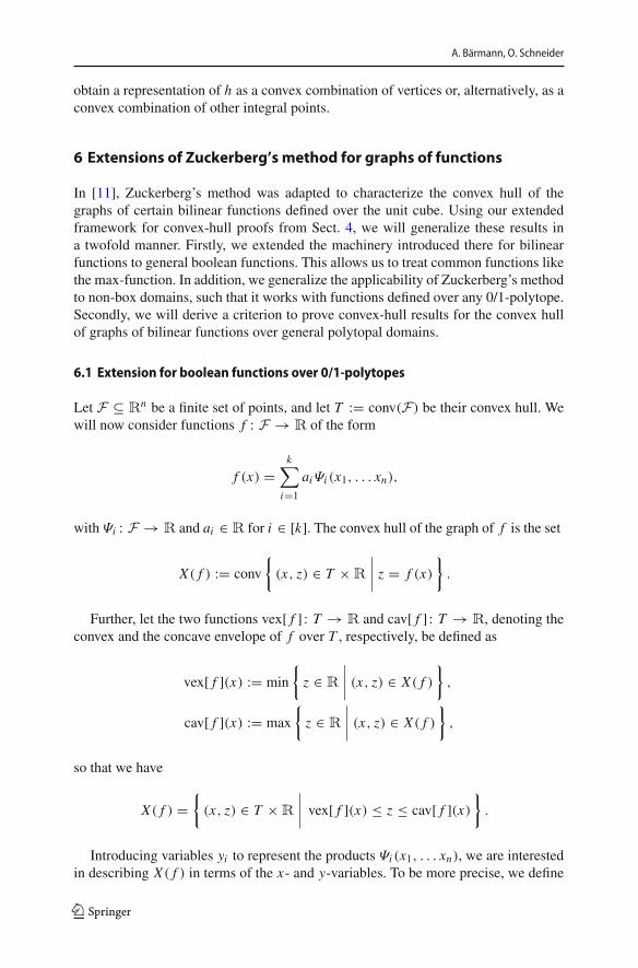
6 Extensions of Zuckerberg’s method for graphs of functions

In [11], Zuckerberg’s method was adapted to characterize the convex hull of thegraphs of certain bilinear functions defined over the unit cube. Using our extendedframework for convex-hull proofs from Sect. 4, we will generalize these results ina twofold manner. Firstly, we extended the machinery introduced there for bilinearfunctions to general boolean functions. This allows us to treat common functions likethe max-function. In addition, we generalize the applicability of Zuckerberg’s methodto non-box domains, such that it works with functions defined over any 0/1-polytope.Secondly, we will derive a criterion to prove convex-hull results for the convex hullof graphs of bilinear functions over general polytopal domains.

6.1 Extension for boolean functions over 0/1-polytopes

Let F ⊆ Rn be a finite set of points, and let T := conv(F) be their convex hull. Wewill now consider functions f : F → R of the form

f (x) =k∑

i=1

aiΨi (x1, . . . xn),

with Ψi : F → R and ai ∈ R for i ∈ [k]. The convex hull of the graph of f is the set

X( f ) := conv

{(x, z) ∈ T × R

∣∣∣∣ z = f (x)

}.

Further, let the two functions vex[ f ] : T → R and cav[ f ] : T → R, denoting theconvex and the concave envelope of f over T , respectively, be defined as

vex[ f ](x) := min

{z ∈ R

∣∣∣∣ (x, z) ∈ X( f )

},

cav[ f ](x) := max

{z ∈ R

∣∣∣∣ (x, z) ∈ X( f )

},

so that we have

X( f ) ={

(x, z) ∈ T × R

∣∣∣∣ vex[ f ](x) ≤ z ≤ cav[ f ](x)

}.

Introducing variables yi to represent the products Ψi (x1, . . . xn), we are interestedin describing X( f ) in terms of the x- and y-variables. To be more precise, we define

123


a function π [ f ] : Rn × Rk → Rn+1 via

π [ f ](x, y) =(

x,

k∑i=1

ai yi

)

and extend it to the power set of Rn × Rk in a canonical fashion:

π [ f ](P) ={

π [ f ](x, y)

∣∣∣∣ (x, y) ∈ P

}

for every P ⊆ Rn × Rk . For a polytope P , let the functions LBP [ f ] : T → R andUBP [ f ] : T → R be defined as

LBP [ f ](x) = min

{k∑

i=1

ai yi

∣∣∣∣ (x, y) ∈ P

}=min

{z ∈ R

∣∣∣∣ (x, z) ∈ π [ f ](P)

},

UBP [ f ](x) = max

{k∑

i=1

ai yi

∣∣∣∣ (x, y) ∈ P

}=max

{z ∈ R

∣∣∣∣ (x, z) ∈ π [ f ](P)

},

respectively, so that

π [ f ](P) ={

(x, z) ∈ T × R

∣∣∣∣ LBP [ f ](x) ≤ z ≤ UBP [ f ](x)

}.

The goal is to give a criterion which allows to prove X( f ) = π [ f ](P) for somegiven function f and polytope P , which is equivalent to vex[ f ](x) = LBP [ f ](x) andcav[ f ](x) = UBP [ f ](x) for all x ∈ T . To this end, we define the set

Z(x) :={

(S1, . . . , Sn) ∈ Ln∣∣∣∣ μ(Si ) = xi ∀i ∈ [n],

ϕ(t, S1, . . . , Sn) ∈ F ∀t ∈ U

}.

It contains all tuples of admissible sets S1, . . . , Sn which express some point x ∈[0, 1]n via the vertices of F using Zuckerberg’s certificate. Finally, let the function� : Ln × RF → U ,

�(S1, . . . , Sn, Ψ ) := μ

({t ∈ U

∣∣∣∣ Ψ (ϕ(t, S1, . . . , Sn)) = 1

})

measure the size of the support of Ψ ◦ ϕ for some Φ : F → R and some fixed(S1, . . . Sn) ∈ Ln . The proof of π [ f ](P) = X( f ) can be split up into π [ f ](P) ⊆X( f ) and X( f ) ⊆ π [ f ](P). The first inclusion is often comparably easy to prove,and for the validity of the second inclusion we give the following criterion.

123


Table 2 Simplifications of �(S1, . . . , Sn , Ψ ) for specific boolean Ψ functions

Ψ Corresp. Boolean operator Simplified �

min(xi , x j ) AND μ(Si ∩ S j )

max(xi , x j ) OR μ(Si ∪ S j )

xi XOR x j XOR μ((Si ∩ S j ) ∪ (Si ∩ S j ))

min(x1, . . . , xn) AND μ(S1 ∩ · · · ∩ Sn)

max(x1, . . . , xn) OR μ(S1 ∪ · · · ∪ Sn)

Theorem 11 If F ⊆ {0, 1}n and f = ∑ki=1 aiΨi , with Ψi : {0, 1}n → {0, 1} and

ai ∈ R for i ∈ [k], we have

vex[ f ](x) = min

⎧⎨⎩

∑i∈[k]

ai�(S1, . . . , Sn, Ψi )

∣∣∣∣ (S1, . . . , Sn) ∈ Z(x)

⎫⎬⎭ ,

cav[ f ](x) = max

⎧⎨⎩

∑i∈[k]

ai�(S1, . . . , Sn, Ψi )

∣∣∣∣ (S1, . . . , Sn) ∈ Z(x)

⎫⎬⎭

for all x ∈ T . In particular, for a polytope P ⊆ Rn+k with π [ f ](P) ⊆ X( f ) wehave π [ f ](P) = X( f ) iff for every x ∈ T there are sets (S1, . . . , Sn) ∈ Z(x) and(S′

1, . . . , S′n) ∈ Z(x) with

∑i∈[k]

ai�(S1, . . . , Sn, Ψi ) = LBP [ f ](x),

∑i∈[k]

ai�(S′1, . . . , S′

n, Ψi ) = UBP [ f ](x).

Theorem 11 gives us a Zuckerberg-type characterization of vex[ f ] and cav[ f ]. Toapply it, we need to design for a general point x ∈ T the sets S1, . . . , Sn ∈ Z(x)

such that∑

i∈[k] ai�(S1, . . . , Sn, Ψi ) is minimized and S′1, . . . , S′

n ∈ Z(x) such that∑i∈[k] ai�(S′

1, . . . , S′n, Ψi ) is maximized. The proof of Theorem 11 is given in the

online supplement [7].The expression �(S1, . . . , Sn, Ψ ) can be made more tractable when some specific

functionsΨ is given. Consider, for instance,Ψ (x1, x2) = x1x2. Thenwe can simplify:

�(S1, S2, Ψ ) = μ(

{t ∈ U

∣∣∣∣ φ(t, S1)φ(t, S2) = 1

}) = μ(S1 ∩ S2).

We exemplarily give similar representations for�(S1, . . . , Sn, Ψ ) for some furtherBoolean functions in Table 2.

A specialization of Theorem 11 for the case F = {0, 1}n and f (x) =∑1≤i< j≤n ai j xi x j was proved in [11] using the above simplification. In the follow-

123


ing, we will demonstrate how to use Theorem 11 to give convex-hull proofs for moregeneral domains and functions.

6.1.1 Convex-hull proofs for polytopal domain

Generalizing an example given in [11] for unit-box domains, we show here how tocharacterize the McCormick-relaxation of the product of two binary variables overa non-box binary polytope. Let F := {x ∈ {0, 1}2 | x1 + x2 ≥ 1} and f : F →{0, 1}, f (x1, x2) = x1x2, and let

P :={

(x1, x2, z) ∈ [0, 1]3∣∣∣∣ z ≤ x1, z ≤ x2, z ≥ x1 + x2 − 1, x1 + x2 ≥ 1

}.

The direction π [ f ](P) ⊆ X( f ) can easily be verified by checking if the extremepoints of X( f ), namely (0, 1, 0), (1, 0, 0) and (1, 1, 1), are feasible for P . For thereverse direction, we plug in the simplification of � for f given in Table 2 intoTheorem 11. We deduce that we need to find two sets S1 and S2 which fulfil

μ(S1 ∩ S2) ≤ min{x1, x2}.

It follows cav[ f ](x) ≤ min{x1, x2}, and with S1 := [0, x1) and S2 := [0, x2) wesee that this bound is attained for all x ∈ conv(F). Therefore, the concave envelopeof f is given by the inequalities z ≤ x1 and z ≤ x2. Similarly,

μ(S1 ∩ S2) ≥ x1 + x2 − 1

leads to the bound vex[ f ](x) ≥ x1 + x2 − 1, and with S1 := [0, x1) and S2 :=[1− x2, 1) it is attained for all x ∈ conv(F). Thus, the convex envelope of f is givenby z ≥ x1 + x2 − 1. Finally, the constraint x1 + x2 ≥ 1 is needed for the initialrestriction of the domain.

6.1.2 Convex-hull proofs for general functions

Now we present an example for the max-function, which shows that our frameworkis applicable to more general functions than the bilinear functions studied in [11]. Weconsider the case f : {0, 1}n → {0, 1}, f (x) = max(x1, . . . , xn) and

P :={

(x1, . . . , xn, z) ∈ [0, 1]n+1∣∣∣∣ z ≤ x1 + · · · + xn, z ≤ 1, z ≥ xi ∀i ∈ [n]

}.

As in the previous example, it is straightforward to verify π [ f ](P) ⊆ X( f ). Forthe converse, we use the simplification for f given in Table 2 to see that the setsS1, . . . , Sn need to fulfil

μ(S1 ∪ · · · ∪ Sn) ≤ min {x1 + · · · + xn, 1}

123


in order to satisfy Theorem 11. Consequently, we have cav[ f ](x) ≤ min{x1 + · · · +xn, 1}. With S1 := [0, x1) and Si := [xi−1, xi−1 + xi ) mod 1 for i ∈ {2, . . . , n}, thisbound is attained for all x ∈ [0, 1]n . Therefore, the concave envelope of f is given byz ≤ x1 + · · · + xn and z ≤ 1. Furthermore, from

μ(S1 ∪ · · · ∪ Sn) ≥ max{x1, . . . , xn}

we obtain the bound vex[ f ](x) ≥ max{x1, . . . , xn}, and setting Si := [0, xi ) fori ∈ {1, . . . , n} makes it tight for all x ∈ [0, 1]n . Thus, the convex envelope of f isgiven by z ≥ xi for i ∈ {1, . . . , n}.

6.2 Extension for bilinear functions over general polytopes

Finally, we derive a generalization of the results from [11] which allows us to computethe convex hull of the graph of a bilinear function over a general polytopal domain T .We start by defining the set

Z(x) :={

(S1, . . . , Sn) ∈ (LU )n∣∣∣∣ μU (Si ) = xi for all i ∈ [n],

ϕU (t, S1, . . . , Sn) ∈ F ∀t ∈ U

},

which contains all admissible sets S1, . . . , Sn for Theorem 11. Furthermore, let thetwo functions ψ−, ψ+ : P → R with

ψ−(x) = min

⎧⎨⎩

∑ξ∈F

μU (LUξ (S1, . . . , Sn)) f (ξ)

∣∣∣∣ (S1, . . . , Sn) ∈ Z(x)

⎫⎬⎭ ,

ψ+(x) = max

⎧⎨⎩

∑ξ∈F

μU (LUξ (S1, . . . , Sn)) f (ξ)

∣∣∣∣ (S1, . . . , Sn) ∈ Z(x)

⎫⎬⎭

encode the convex and concave envelope, respectively, in a Zuckerberg fashion. Wenow derive an auxiliary representation of X( f ) in terms of these two functions.

Lemma 3 For every function f : F → R, we have

X( f ) ={

(x, z) ∈ T × R

∣∣∣∣ ψ−(x) ≤ z ≤ ψ+(x)

}.

Proof First, assume (x, z) ∈ X( f ). This means

(x, z) =|F |∑k=1

λk(ξk, f (ξ k))

for some λk ≥ 0 for k = 1, . . . , |F | with∑|F |

k=1 λk = 1 and a fixed orderingξ1, . . . , ξ |F | of F . The sets Si ∈ LU with μU (Si ) = xi are defined exactly as in

123


the proof of Theorem 6: for the partition U = I1 ∪ · · · ∪ I|F | with I1 = [0, λ1) andIk = [λ1 + · · · + λk−1, λ1 + · · · + λk) for k ∈ {2, . . . , |F |}, we set

Si =⋃

k: ξ ki =0

(Ik, ξki ).

For every k = 1, . . . , |F |, we have LUξ k (S1, . . . , Sn) = Ik , and consequently

μU (LUξ k (S1, . . . , Sn)) = λk . With

z =|F |∑k=1

λk f (ξ k) =|F |∑k=1

μU (LUξ k (S1, . . . , Sn)) f (ξ k),

it follows that ψ−(x) ≤ z ≤ ψ+(x).For the converse, assume ψ−(x) ≤ z ≤ ψ+(x) and let (S1, . . . , Sn) and

(S′1, . . . , S′

n) be optimizers for the minima and maxima defining ψ−(x) and ψ+(x)

respectively. We write z = tψ−(x) + (1 − t)ψ+(x) for some t ∈ [0, 1] and set

λ(ξ) := tμU (LUξ (S1, . . . , Sn)) + (1 − t)μU (LU

ξ (S′1, . . . , S′

n))

for all ξ ∈ F . This yields a representation of (x, z) as the convex combination

(x, z) =∑ξ∈F

λ(ξ)(ξ, ψ(ξ)).

��With Lemma 3, we can express the convex hull of the graph of a function via

functions defined over Zuckerberg sets. We will now make these abstract expressionsmore concrete for the case of bilinear functions. For this purpose, we consider anarbitrary bilinear function

f : F → R, f (x) =k∑

i j∈E

ai j xi x j (34)

with coefficients ai j ∈ R and a subset E ⊆ {(i, j) ∈ N2 | 1 ≤ i < j ≤ n}.Furthermore, we define the function M : (LU )2 → R in Fig. 13, which measures akind of generalized overlap between two sets S1, S2 ∈ LU .

For the particular case of a bilinear function f , Lemma 3 yields the followingcharacterizations of cav[ f ](x) and vex[ f ](x).

Theorem 12 For the bilinear function f of the form (34), we have

vex[ f ](x) = min

⎧⎨⎩

∑i j∈E

ai j M(Si , S j )

∣∣∣∣ (S1, . . . , Sn) ∈ Z(x)

⎫⎬⎭ ,

123


Fig. 13 The function M : (LU )2 → R

cav[ f ](x) = max

⎧⎨⎩

∑i j∈E

ai j M(Si , S j )

∣∣∣∣ (S1, . . . , Sn) ∈ Z(x)

⎫⎬⎭

for all x ∈ T . In particular, for a polytope P ⊆ Rn(n+1)/2 with π [ f ](P) ⊆ X( f ), wehave π [ f ](P) = X( f ) if and only if for every x ∈ T there are sets (S1, . . . , Sn) ∈Z(x) and (S′

1, . . . , S′n) ∈ Z(x) with

∑i j∈E

ai j M(Si , S j ) = LBP [ f ](x),

∑i j∈E

ai j M(S′i , S′

j ) = UBP [ f ](x).

Proof We observe that

∑ξ∈F

μU (LUξ (S1, . . . , Sn)) f (ξ) =

∑ξ∈F

μU (LUξ (S1, . . . , Sn))

∑i j∈E

ai jξiξ j

=∑i j∈E

ai j

∑ξ∈F

μU (LUξ (S1, . . . , Sn))ξiξ j

=∑i j∈E

ai j M(Si , S j ).

��

Theorem 12 allows us to give compact representations for vex[ f ] and cav[ f ] overpolytopal domains. To do so, we need to design suitable sets S1, . . . , Sn ∈ Z such that∑

i j∈E ai j M(Si , S j ) is minimized and S′1, . . . , S′

n ∈ Z such that∑

i j∈E ai j M(S′i , S′

j )

is maximized, both for an arbitrary point x ∈ Rn .

123


6.2.1 Convex-hull proofs for non-0/1 domain

We can use Theorem 12 to prove again that X( f ) for f (x1, x2) = x1x2 is given by theMcCormick-inequalities. However, we will now do this over the bounds 0 ≤ x1 ≤ u1and 0 ≤ x2 ≤ u2 for u1, u2 ≥ 0 instead of the unit bounds as in Sect. 2.1. Let

P :={

(x1, x2, z) ∈ R3∣∣∣∣ z ≤ u2x1, z ≤ u1x2, z ≥ 0, z ≥ u2x1 + u1x2 − u1u2

}.

The direction π [ f ](P) ⊆ X( f ) can easily be verified.For the reverse direction, we conclude from

M(S1, S2) ≤ u1u2 min

{1

u1x1,

1

u2x2

}(35)

that cav[ f ](x) ≤ {(1/u1)x1, (1/u2)x2}, and with S1 = ([0, x1/u1), u1), S2 =([0, x2/u2), u2) this bound is attained for all x1 ∈ [0, u1], x2 ∈ [0, u2]. Therefore, theconcave envelope is given by z ≤ u2x1 and z ≤ u1x2. In a similar fashion, it followsfrom

M(S1, S2) ≥ u1u2 max

{0,

1

u1x1 + 1

u2x2 − 1

}(36)

that vex[ f ](x) ≥ max{0, (1/u1)x1 + (1/u2)x2 − 1}. By choosing the sets S1 =([0, x1/u1), u1), S2 = ([1 − x2/u2, 1), u2) we can show that this bound is attainedfor all x1 ∈ [0, u1], x2 ∈ [0, u2]. Thus, the convex envelope is given by z ≥ 0 andz ≥ u2x1 + u1x2 − u1u2.

7 Conclusion

We have presented a vastly simplified framework for Zuckerberg’s geometric prooftechnique for convex-hull results. By restating the method in terms of our notion of setcharacterizations, we were able to accomplish several benefits. Firstly, we have iden-tified three major strategies one can pursue in Zuckerberg-type convex-hull proofs.This underlines the high flexibility in devising algorithmic schemes the method offers.Secondly, we have significantly extended the expressive power of Zuckerberg’s tech-nique by basing it on a different underlying subset algebra. It can now be used tocharacterize the convex hulls of general convex sets, including, but not limited to inte-ger polyhedra. Using this extension, we give characterizations of the convex hull ofBoolean and bilinear functions over polytopal domains. Finally, we have given a vari-ety of indicative examples for the use of our framework with the intention to conveythe ideas as hands-on as possible.

Wefind it a very interesting avenue for future research to develop further algorithmicstrategies for Zuckerberg proofs and to extend the scope of those we have introduced.For example, one could not only consider linear programs but pass to (mixed-)integer

123


oneswhen following the technique using feasibility subproblems. Thismight entail theconsideration of minimally infeasible subsystems to verify the set characterizations.

Altogether, we make a strong case for the canonization of Zuckerberg’s proof tech-nique in standard text books on integer programming and polyhedral combinatorics.We are certain it will enable many more interesting convex-hull results in the future.

Supplementary Information The online version contains supplementary material available at https://doi.org/10.1007/s10107-021-01705-3.

Acknowledgements We thank Alexander Martin and Thomas Kalinowski for our fruitful discussions onthe topic.

Funding Open Access funding enabled and organized by Projekt DEAL.

OpenAccess This article is licensedunder aCreativeCommonsAttribution 4.0 InternationalLicense,whichpermits use, sharing, adaptation, distribution and reproduction in any medium or format, as long as you giveappropriate credit to the original author(s) and the source, provide a link to the Creative Commons licence,and indicate if changes were made. The images or other third party material in this article are includedin the article’s Creative Commons licence, unless indicated otherwise in a credit line to the material. Ifmaterial is not included in the article’s Creative Commons licence and your intended use is not permittedby statutory regulation or exceeds the permitted use, you will need to obtain permission directly from thecopyright holder. To view a copy of this licence, visit http://creativecommons.org/licenses/by/4.0/.

References

1. Bienstock, D., Zuckerberg, M.: Subset algebra lift operators for 0–1 integer programming. SIAM J.Optim. 15(1), 63–95 (2004)

2. Bienstock, D., Zuckerberg, M.: Simpler derivation of bounded pitch inequalities for set covering, andminimum knapsack sets. arXiv preprint arXiv:1806.07435 (2018)

3. Bärmann, A., Gellermann, T., Merkert, M., Schneider, O.: Staircase compatibility and its applicationsin scheduling and piecewise linearization. Discrete Optim. 29, 111–132 (2018)

4. Bärmann, A., Gemander, P., Martin, A., Merkert, M.: On recognizing staircase compatibility. http://www.optimization-online.org/DB_FILE/2020/12/8138.pdf (2020)

5. Bärmann, A., Gemander, P., Merkert, M.: The clique problem with multiple-choice constraints undera cycle-free dependency graph. Discrete Appl. Math. 283, 59–77 (2020)

6. Bärmann, A., Martin, A., Schneider, O.: The bipartite Boolean quadric polytope with multiple-choiceconstraints. http://www.optimization-online.org/DB_FILE/2020/09/8033.pdf (2020)

7. Bärmann, A., Schneider, O.: Supplementary materials: set characterizations and convex extensions forgeometric convex-hull proofs (2020)

8. Chudnovsky, M., Robertson, N., Seymour, P., Thomas, R.: The strong perfect graph theorem. Ann.Math. 164(1), 51–229 (2006)

9. Fiorini, S., Huynh, T.,Weltge, S.: Strengthening convex relaxations of 0/1-sets using boolean formulas.Math. Program. 1–16 (2020)

10. Fulkerson, D., Gross, O.: Incidence matrices and interval graphs. Pac. J. Math. 15(3), 835–855 (1965)11. Gupte, A., Kalinowski, T., Rigterink, F., Waterer, H.: Extended formulations for convex hulls of some

bilinear functions. Discrete Optim. 36, 100569 (2020)12. Harris, M., Kalinowski, T.: Convex hulls for graphs of quadratic functions with unit coefficients: even

wheels and complete split graphs. arXiv preprint arXiv:2007.05656 (2020)13. Hoàng, C.T.: Alternating orientation and alternating colouration of perfect graphs. J. Comb. Theory

Ser. B 42(3), 264–273 (1987)14. Hoffman, A.J., Kruskal, J.B.: Linear Inequalities and Related Systems, Chap. Integral Boundary Points

of Convex Polyhedra, pp. 223–246. Princeton University Press, Princeton (1956)

123

https://doi.org/10.1007/s10107-021-01705-3

https://doi.org/10.1007/s10107-021-01705-3

http://creativecommons.org/licenses/by/4.0/

http://arxiv.org/abs/1806.07435

http://www.optimization-online.org/DB_FILE/2020/12/8138.pdf



http://arxiv.org/abs/2007.05656


15. Krarup, J., Bilde, O.: Numerische Methoden bei Optimierungsaufgaben: Optimierung bei graphenthe-oretischen und ganzzahligen Problemen, Vol. 3, Chap. Plant Location, Set Covering and EconomicLot Size: An O(mn)-Algorithm for Structured Problems, pp. 155–180. Birkhäuser, Basel (1977)

16. Lovász, L., Schrijver, A.: Cones of matrices and set-functions and 0–1 optimization. SIAM J. Optim.1(2), 166–190 (1991)

17. Mahjoub, A.R.: On the stable set polytope of a series–parallel graph. Math. Program. 8, 53–57 (1988)18. Padberg, M.: The Boolean quadric polytope: some characteristics, facets and relatives. Math. Program.

45(1–3), 139–172 (1989)19. Pochet, Y.,Wolsey, L.A.: Production Planning byMixed Integer Programming. Springer, Berlin (2006)20. Sridhar, S., Linderoth, J., Luedtke, J.: Locally ideal formulations for piecewise linear functions with

indicator variables. Oper. Res. Lett. 41(6), 627–632 (2013)21. Zuckerberg, M.: A Set Theoretic Approach to Lifting Procedures for 0, 1 Integer Programming.

Columbia University, New York (2004). (Ph.D. thesis)22. Zuckerberg, M.: Geometric proofs for convex hull defining formulations. Oper. Res. Lett. 44(5), 625–

629 (2016)

Publisher’s Note Springer Nature remains neutral with regard to jurisdictional claims in published mapsand institutional affiliations.

123

Documents

Set characterizations and convex extensions for geometric