SET IDENTIFIED DYNAMIC ECONOMIES AND ROBUSTNESSTO MISSPECIFICATION

ANDREAS TRYPHONIDESHUMBOLDT UNIVERSITY

Abstract. We propose a new inferential methodology for dynamic economies thatis robust to misspecification of the mechanism generating frictions. Economies withfrictions are treated as perturbations of a frictionless economy that are consistentwith a variety of mechanisms. We derive a representation for the law of motion forsuch economies and we characterize parameter set identification. We derive a linkfrom model aggregate predictions to distributional information contained in quali-tative survey data and specify conditions under which the identified set is refined.The latter is used to semi-parametrically estimate distortions due to frictions inmacroeconomic variables. Based on these estimates, we propose a novel test forcomplete models. Using survey data collected by the European Commission, weapply our method to estimate distortions due to financial frictions in the Span-ish economy. We investigate the implications of these estimates for the adequacyof the standard model of financial frictions SW-BGG (Smets and Wouters (2007),Bernanke, Gertler, and Gilchrist (1999)).

Keywords: Frictions, Heterogeneity, Set Identification, Surveys, Testing

JEL Classification: C13, C51, C52, E10, E60

Date: 5/01/2018.This paper is based on chapter 2 of my PhD thesis (European University Institute). I thank Fabio Canova for hisadvice and help with earlier versions of this paper, and the rest of the thesis committee: Peter Reinhard Hansen,Frank Schorfheide and Giuseppe Ragusa for comments and suggestions. This paper benefited also from discussionswith George Marios Angeletos, Eric Leeper, Ellen McGrattan, Juan J. Dolado, Thierry Magnac, Manuel Arellano,Eleni Aristodemou, Raffaella Giacomini, and comments from participants at the 2nd IAAE conference, the 30th EEACongress, T2M -BdF workshop, the ES Winter Meetings, the seminars at the University of Cyprus, Royal Holloway,Humboldt University, Universidad Carlos III, University of Glasgow, University of Southampton, the Econometricsand Applied Macro working groups at the EUI. Any errors are my own.

1

1. Introduction

Incorporating frictions in dynamic macroeconomic models is undoubtedly essential,

both in terms of their theoretical and empirical implications. They are being rou-

tinely used to explain both the observed persistence of macroeconomic time series

and several stylized facts obtained from firm and household level data. However, at

the macroeconomic level, the selection between different types of frictions and the

specification of their corresponding mechanism is a complicated process featuring ar-

bitrary aspects. This arbitrariness implies that different studies may find support for

alternative types of frictions, depending on other assumptions made. For example,

the choice of nominal rigidities might depend on which real rigidities are included

in the model or whether there is variable capital utilization or not1. More impor-

tantly, unless frictions are micro-founded, policy conclusions may become whimsical

as different mechanisms imply different relationships between policy parameters and

economic outcomes.

In this paper we propose a new inferential methodology that is robust to misspecifi-

cation of the mechanism generating frictions in a dynamic stochastic economy. The

approach treats economies with frictions as perturbations of a frictionless economy,

which are not uniquely pinned down, and are consistent with different structural

specifications.

The paper makes several contributions. First, we derive a characterization for the

law of motion of an economy with frictions that imposes identifying restrictions on

the solution of the model. Chari, Kehoe, and McGrattan (2007), CKM hereafter,

identify wedges in the optimality conditions of a frictionless model that produce the

same equilibrium allocations in economies with specific parametric choices for the

1See the analysis of Christiano, Eichenbaum, and Evans (2005) and their comparison to the resultsof Chari, Kehoe, and McGrattan (2000).

2

frictions. We also take a frictionless model as a benchmark but contrary to CKM we

construct a general representation for the wedge in the decision rules. We illustrate

through examples that the sign of the conditional mean of the decision rule wedge is

typically known, even when the exact mechanism generating the friction is unknown.

We utilize knowledge of the sign of the conditional mean to set-identify the parameters

of the benchmark model.

Moment inequality restrictions have been used to characterize frictions in specific

markets, see for example Luttmer (1996) and Chetty (2012). To our knowledge, we are

the first to characterize such restrictions in dynamic stochastic macroeconomic models

and to show their relationship with the literature on wedges in equilibrium models.

We are also the first to characterize set identification in this class of models. The

econometric theory we develop can accommodate inequality restrictions of general

form.

Due to set identification, many models with frictions are likely to be consistent with

the robust identifying restrictions. Thus, additional data other than macroeconomic

time series can be potentially useful in order to further constrain the set of admissible

models. As a second contribution, our methodology permits the introduction of

additional restrictions. We show how qualitative survey data can be useful for this

purpose, since they provide distributional information which is highly relevant in

models featuring frictions and heterogeneity. More specifically, qualitative survey data

are linked to current and future beliefs of agents in the model. If survey data reflect

subjective conditional expectations, they contain important indications about agents’

actions through the behavioral equations. In the literature2, survey data are typically

linked to model based random variables using additional observation equations with

2We mainly refer to the treatment of survey data in the most recent "modern" DSGE literature. Thetreatment of survey data in Rational Expectations models date back to the work of Pesaran (1987)and others.

3

additive measurement error (see e.g. Del Negro and Schorfheide (2013)). However,

this paper follows a different approach as the model is incomplete and there is no

well defined model quantity that can be linked to the data. This is where the law

of motion representation we derive proves useful, as we can link the macroeconomic

distortions to aggregated qualitative surveys through additional moment inequality

restrictions.

Regarding possible applications of the methodology, we show how it contributes to

model selection, where the object of interest is not the set-identified parameter vector

itself, but the implied semi-parametric estimates of frictions. To that end we propose

a novel Wald test that compares the estimates of distortions implied by a candidate

model to the robust set obtained using our method. We also derive large sample

theory for this type of test. Beyond restricting the set of observationally equivalent

distortions, the use of additional data i.e. surveys, prevents the test statistic from

degenerating when the data generating process is such that the incomplete model

nests the candidate model.

We apply the methodology to estimate the distortions present in the Spanish economy

due to financial frictions. We estimate a small open economy version of the Smets

and Wouters (2007) model using qualitative survey data collected by the Commission

on the financial constraints of firms. We contrast the implied estimates of distortions

to macroeconomic aggregates due to these frictions to those identified using a com-

plete model that incorporates the Bernanke, Gertler, and Gilchrist (1999) financial

accelerator.

We have already referred to how our paper relates to some strands of literature,

namely the literature on wedges and frictions (i.e. Chari, Kehoe, and McGrattan

(2007), Christiano, Eichenbaum, and Evans (2005), Chari, Kehoe, and McGrattan

(2000)) and the literature on including survey data in DSGE models (i.e. Del Negro4

and Schorfheide (2013)). We contribute to the literature that deals with partial iden-

tification in structural macroeconomic models (e.g. Lubik and Schorfheide (2004);

Coroneo, Corradi, and Santos Monteiro (2011)) and the literature on applications

of moment inequality models, see Pakes, Porter, Ho, and Ishii (2015) and references

therein. We postpone illustrating more detailed connections to the vast partial iden-

tification literature for later sections, when we deal with estimation and inference

using our methodology.

The rest of the paper is organized as follows. Section 2 provides a motivating ex-

ample of the methodology in a partial equilibrium context, while section 3 presents

the prototype economy which will be used as an experimental lab to illustrate our

methodology. Section 4 examines the distortions present in the decision rules and

their observable aggregate implications. Section 5 provides the formal treatment of

identification without additional information while Section 6 analyzes the case with

additional information, including qualitative survey data. Section 7 discusses infer-

ence issues and provides the test. Section 8 contains the application to Spanish data

and Section 9 concludes and provides avenues for future work. Appendix A contains

proofs and the empirical results. Appendix B (online) contains more examples of

moment inequality restrictions, details on the relation to the model uncertainty liter-

ature and the algorithm to compute frictions, an example on identification using our

method, an illustration of the validity of bootstrap for the proposed test and a plot

of the survey data used in the application.

Throughout the paper we refer to three different conditional probability measures.

The objective probability measure, Pt, the probability measure determined by the

frictionless model Mf , PMf

t p.|, .q, and the subjective probability measure Pt,i where i

identifies agent i and t the timing of the conditioning set. All three are absolutely5

continuous with respect to Lebesgue measure. The corresponding conditional expec-

tation operators are Etp.q, EMf

t p.|.q and Ei,tp.q. We distinguish between the first and

the second conditional expectation as the model will be correctly specified only if

the econometrician employs the right DGP. Moreover, T denotes the length of both

the aggregate and average survey data, and L the number of agents. We denote by

θ P Θ the parameters of interest with ΘCSα the corresponding 1 ´ α level confidence

set, and by qjp; θq a measurable function. Bold capital letters e.g. Yt denote a vector

of length τ containing tYjujďτ . The operator Ñp signifies convergence in probability

and the operator Ñd convergence in distribution; N p., .q is the Normal distribution

whose cumulative is Φp., .q; ||.|| is the Euclidean norm unless otherwise stated; K

signifies the orthogonal complement and H the empty set. We denote by pΩ,Sy,Pq

the probability triple for the observables to the econometrician, where Sy “ σpY q, is

the sigma-field generated by Y and pΩ,F , tFutě0,Pq the corresponding filtered prob-

ability space. Finally we denote by d and m the Hadamard product and division

respectively.

2. Robustness in Partial Equilibrium

We first motivate our approach by illustrating the special case of observing a single

household receiving a random exogenous endowment yi,t and making consumption-

savings decisions pci,t, si,tq in a partial equilibrium context. As in Zeldes (1989), wealth

wi,t earns a riskless return R and there is a borrowing limit at zero:

maxtci,tu

8t“1

E0

8ÿ

t“1βtc1´ωi,t ´ 11´ ω

s.t. yi,t “ si,t ` ci,t

wi,t`1 “ Rwi,t ` si,t

wi,t`1 ě 06

The corresponding consumption Euler equation is distorted by the non-negative

Lagrange multiplier on the occasionally binding liquidity constraint, denoted by

λi,t:

U 1pci,t; θq “ βEtp1` rt`1qU1pci,t`1; θq ` λi,t(1)

Whether the borrowing constraint is binding depends on the household’s expectations

about future income, and therefore on its information set. Consequently, condition (1)

is a conditional moment inequality, and for any conformable variable zi,t that belongs

to the household’s information set, the following unconditional moment inequality

holds:

E rpU 1pci,t; θq ´ βp1` rt`1qU1pcit`1; θqq b zi,ts ě 0(2)

Given the inequality, there is no unique vector pθ, βq that satisfies it, and we therefore

no longer have point identification. In order to derive explicit identification regions,

we adopt the approximation of Hall (1978), which for CRRA utility and constant

interest rate implies the following law of motion for consumption:

ci,t`1 “ µci,t ` εi,t`1 ` λi,t(3)

where λi,t ” ´pU2pci,t`1qq´1λi,t. Since µ may be exceed one if βR ą 1 and vice verca3,

we re-express 3 in terms of consumption growth, ∆ci,t`1 “ µci,t ` εt`1 ` λi,t.

Since the sign of Etλt is still positive, the identified set for µ0 is :

µID,1 :“ˆ

0, 1` Ezi,t∆ci,t`1

Ezi,tci,t

“ p0, 1` µs(4)

As we can readily see from (4), the inherent unobservability of λi,t is the root of

the loss of point identification of µ0. An interesting question is whether additional

3In fact, µ is equal to pβp1` rqq´u1pcq

cu2pcq ą 0, and it will be constant for CRRA utility.7

data can be informative about, or even point identify, µ0. The answer in this case is

affirmative.

Suppose that we observe the dichotomous response of the household over time to

a survey question that asks whether the household is (or expects to be) financially

constrained. An honest household will answer positively whenever λi,t ą 0. What

this implies is that the time series of responses tχi,tutďN for χi,t ” 1p1λi,t ą 01q can

be used to estimate Ptpλi,t ą 0q. The conditional probability distribution of ∆ci,t`1,

Ptp∆ci,t`1 ă uq for any u P R is equal to

Ptpεi,t`1 ă u´ µci,tqPtpλi,t “ 0q ` Ptpεi,t`1 ă u´ µci,t ´ λi,tqPtpλi,t ą 0q(5)

For εt`1 „ Np0, σ2ε q, (5) simplifies further to,

Φ0,σ2εpu´ µci,tqPtpλi,t “ 0q ` Φ0,σ2

εpu´ µci,t ´ λi,tqPtpλi,t ą 0q(6)

A key observation is that the distortion λi,t is positive only when the state variables

pwi,t, yi,tq lie in a particular area of their domain A which is determined by an unknown

endogenous threshold pw˚i , y˚i q. A complete model would pin down, analytically or

numerically this domain. Observing χi,t dispenses us with the need to characterize

A. Once the threshold condition is satisfied, λi,t will be a linear(ized) function of

pwi,t, yi,tq.

Moreover, it is also reasonable to assume that λi,t is a function of the unobserved

exogenous shocks εt`1. We can therefore substitute λi,t for λ1ci,t ` λ2εi,t`1, in (6),

which yields the following quantile restriction:

Ptp∆ci,t`1 ă uq “ Φ0,σ2εpu´ µci,tqPtpλi,t “ 0q ` Φ0,σ2

ε p1`λ2q2pu´ µcolsci,tqPtpλi,t ą 0q

ě Φ0,σ2εpu´ µci,tqPtpλi,t “ 0q ` Φ0,σ2

olspu´ µolsci,tqPtpλi,t ą 0q(7)

8

where µcols is equivalent to the least squares estimate in the case of borrowing con-

straints with probability one. The inequality is derived for a class of functions

Ptpλi,t ą 0q.

How does this additional inequality refine the identified set in (4)? Denote by µID,2

the set of µ consistent with the unconditional moment inequality constructed using

zt and (7). The simplest way to show the refinement of (4) is to show that there

exists a µ P µID,1 that does not belong to µID,2. For simplicity, let µ0 “ 0, which

implies that ∆ci,t`1 “ χi,tpλ1ci,t ` λ2εi,t`1q ` p1 ´ χi,tqεi,t`1. This is equivalent to

considering an economy in which βp1 ` rq ă 1 and the consumer has very high risk

aversion (ω Ñ 8). In Appendix A we show that using µols as the test point, (7)

is not satisfied for pt “ 1pci,t ă 0q, and therefore µols R µID,2. The upper bound in

µID should thus be lower than µols. In words, as long as the agent has some positive

unconditional probability of not being constrained (here 12), observing her responses

provides additional information.

The identified set for the reduced form, µID “ µID,1XµID,2, is informative in different

ways. First, as already mentioned, given µID, we can recover the implied identified set

for the risk aversion parameter, ωID. As is typical in the empirical macro literature,

pr, βq are not identified from the dynamic properties of the model but rather from

other information, i.e steady states. In the case when βp1 ` rq “ 1, risk aversion

is unidentified, ωID “ R`, as consumption follows a random walk. For βp1 ` rq ‰

1,

ωID :“"

ω P R` X„

logpβp1` rqqlog p1` µuIDq

,logpβp1` rqqlog

`

1` µlID˘

*

This interval has a very intuitive interpretation, and actually reflects restrictions on

preferences implied by the presence of non-diversifiable income risk and observed

behavior. For the sake of illustration let us focus on the identified set implied9

by (4). If βp1 ` rq ă 1, the household is impatient and does not accumulate

wealth indefinitely. Using zi,t “ yi,t, since income and consumption growth are neg-

atively correlated, which is usually the case when liquidity constraints are present4,

ωID,1 “!

ω P R` : ω ă logpβp1`rqqlogEyi,tci,t´logpEyi,tci,t´Eyi,t∆ci,t`1q

)

. The stronger the negative

correlation, the lower the upper bound on risk aversion, indicating the fact that the

less risk averse household is not accumulating enough wealth to fully insure against

income risk. On the contrary, weak negative correlation permits higher estimates

of risk aversion. Similar to Arellano, Hansen, and Sentana (2012), the degree of

under-identification therefore depends on this correlation, which is itself a function of

pω, β, rq.

Second, the upper and lower bounds for µID can be used to do inference on other

interesting quantities, including the model itself. For example, we can construct set

estimates of distortions in consumption implied by liquidity constraints by plugging-

in the identified set and averaging over the observations. In population, this produces

an identified set for distortions:

Eλi,t P“

Eci,t`1 ´ µuIDci,t,Eci,t`1 ´ µ

lIDci,t

‰

(8)

Another key observation is that although we have motivated the sign of Etλi,t by

looking at the exogenous constraint of no borrowing, the sign is robust to different

mechanisms, as long as they prevent the household from smoothing consumption. For

example, a non zero constraint on next period wealth, i.e. wi,t`1 ě b or a constraint

that is endogenous, i.e. wi,t`1 ě bpyi,tq where yi,t is the relevant state variable, lead to

an Euler equation which is distorted in the same direction. Therefore, the identified

set of distortions will be a priori consistent with different mechanisms generating

liquidity constraints.

4Deaton (1991)10

A mechanism will not be rejected as long as it generates distortions that will statisti-

cally belong to the identifed set for Eλt. Moreover, we will see that in general equilib-

rium, survey data will generate additional moment restrictions which can potentially

add information. The identified set is expected to be refined, and this refinement can

potentially provide power to reject alternative models that cannot be rejected using

bound (4).

In the rest of the paper we will gradually characterize the case for general equilib-

rium models and what information aggregated surveys can provide, based on similar

assumptions to those made in the simple example. To do so, we will provide below

the benchmark general equilibrium model.

3. Towards General Equilibrium

In the last section we considered liquidity constraints for a single household in a

partial equilibrium context. In this section, we consider additional types of frictions

by including capital and a representative firm in the economy and set up the general

equilibrium framework. Building up from the previous section, consider a simple Real

Business Cycle (RBC) model, in which dynastic households with Constant Relative

Risk Aversion (CRRA) preferences form expectations about key state variables and

make consumption - savings decisions. We denote by Λtpiq the distribution of agents

at time t, and the corresponding aggregate variables by capital letters i.e. Xt ”´xi,tdΛtpiq. Households rent capital pki,tq to a representative firm, which is used for

production, and receive a share pηi,tq of profits made by the firm. Profits are simply

the production of output using capital intensive technology with random productivity

pZtKαt q minus the rents paid to all households pRtKtq, that is, pri,t “ ηi,tpZtK

αt ´

RtKtq. Household income is therefore yi,t “ Rtki,t ` pri,t. Individual investment

decisions pιi,tq increase the availability of capital for next period, up to a certain level11

of depreciation. The household’s optimization problem is therefore as follows:

maxtci,t,ki,t`1,wi,t`1,ιi,tu81

Ei,08ÿ

t“1βtc1´ωi,t ´ 11´ ω

s.t. wi,t`1 “ Rtwi,t ` yi,t ´ ci,t ´ ιi,t

ki,t`1 “ p1´ δqki,t ` ιi,t

Note that individual expectations Ei,0 are not necessarily formed with respect to the

objective probability measure, nor with respect to the same information set. Denote

by ξt the aggregation residual, and by X the percentage deviations of any aggregate

variable Xt from aggregate steady state xss. Then the system of aggregate linearized5

equilibrium and market clearing conditions are as follows:

´ωCt ´ ξC,t ´ βrssEtRt`1 ` ωEtCt`1 “ 0

yssYt ´ cssCt ´ issIt “ 0

Kt`1 ´ p1´ δqKt ´ δIt “ 0

Yt ´ Zt ´ αKt ´ ξY,t “ 0

Rt ´ Zt ` p1´ αqKt ´ ξR,t “ 0

Under approximate linearity, that is, when ξt is negligible 6, we can obtain the ag-

gregate decision rules for Xt, which will depend on predetermined capital ki,t and

on aggregate conditional expectations on productivity for some j periods ahead,

EtZt`j.

5Note that here we follow the linear approximation to the first order conditions as widely used inthe DSGE literature, while in the last section we followed Hall (1978), where the variables are notin percentage deviation from steady state. The analysis is nevertheless largely unaffected.6Absence of frictions is one of the reasons for which approximate linearity holds.

12

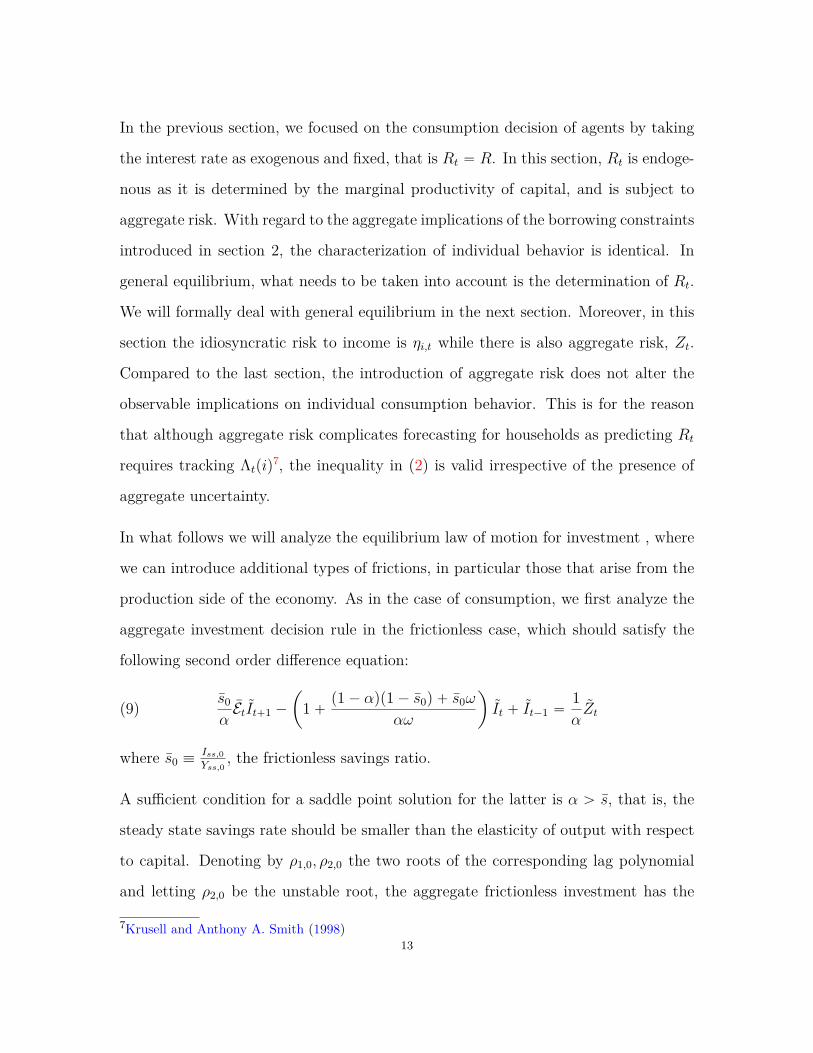
In the previous section, we focused on the consumption decision of agents by taking

the interest rate as exogenous and fixed, that is Rt “ R. In this section, Rt is endoge-

nous as it is determined by the marginal productivity of capital, and is subject to

aggregate risk. With regard to the aggregate implications of the borrowing constraints

introduced in section 2, the characterization of individual behavior is identical. In

general equilibrium, what needs to be taken into account is the determination of Rt.

We will formally deal with general equilibrium in the next section. Moreover, in this

section the idiosyncratic risk to income is ηi,t while there is also aggregate risk, Zt.

Compared to the last section, the introduction of aggregate risk does not alter the

observable implications on individual consumption behavior. This is for the reason

that although aggregate risk complicates forecasting for households as predicting Rt

requires tracking Λtpiq7, the inequality in (2) is valid irrespective of the presence of

aggregate uncertainty.

In what follows we will analyze the equilibrium law of motion for investment , where

we can introduce additional types of frictions, in particular those that arise from the

production side of the economy. As in the case of consumption, we first analyze the

aggregate investment decision rule in the frictionless case, which should satisfy the

following second order difference equation:

(9) s0

αEtIt`1 ´

ˆ

1` p1´ αqp1´ s0q ` s0ω

αω

˙

It ` It´1 “1αZt

where s0 ”Iss,0Yss,0

, the frictionless savings ratio.

A sufficient condition for a saddle point solution for the latter is α ą s, that is, the

steady state savings rate should be smaller than the elasticity of output with respect

to capital. Denoting by ρ1,0, ρ2,0 the two roots of the corresponding lag polynomial

and letting ρ2,0 be the unstable root, the aggregate frictionless investment has the

7Krusell and Anthony A. Smith (1998)13

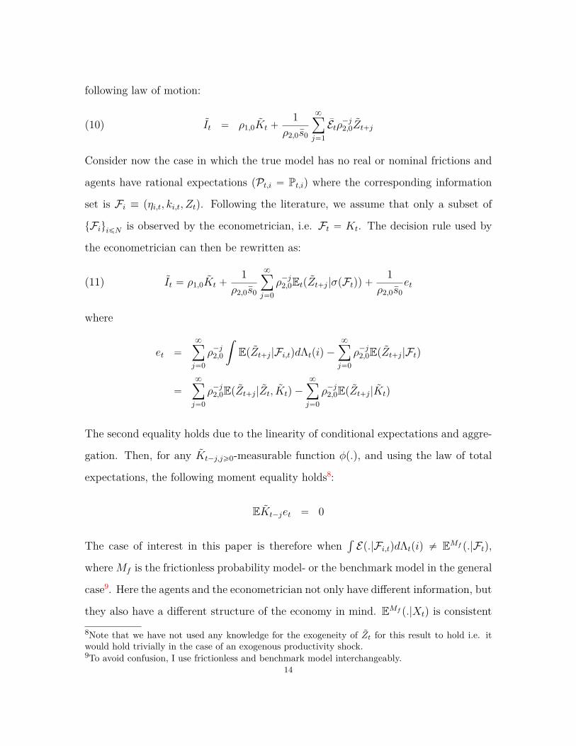
following law of motion:

It “ ρ1,0Kt `1

ρ2,0s0

8ÿ

j“1Etρ´j2,0Zt`j(10)

Consider now the case in which the true model has no real or nominal frictions and

agents have rational expectations (Pt,i “ Pt,i) where the corresponding information

set is Fi ” pηi,t, ki,t, Ztq. Following the literature, we assume that only a subset of

tFiuiďN is observed by the econometrician, i.e. Ft “ Kt. The decision rule used by

the econometrician can then be rewritten as:

(11) It “ ρ1,0Kt `1

ρ2,0s0

8ÿ

j“0ρ´j2,0EtpZt`j|σpFtqq `

1ρ2,0s0

et

where

et “

8ÿ

j“0ρ´j2,0

ˆEpZt`j|Fi,tqdΛtpiq ´

8ÿ

j“0ρ´j2,0EpZt`j|Ftq

“

8ÿ

j“0ρ´j2,0EpZt`j|Zt, Ktq ´

8ÿ

j“0ρ´j2,0EpZt`j|Ktq

The second equality holds due to the linearity of conditional expectations and aggre-

gation. Then, for any Kt´j,jě0-measurable function φp.q, and using the law of total

expectations, the following moment equality holds8:

EKt´jet “ 0

The case of interest in this paper is therefore when´

Ep.|Fi,tqdΛtpiq ‰ EMf p.|Ftq,

whereMf is the frictionless probability model- or the benchmark model in the general

case9. Here the agents and the econometrician not only have different information, but

they also have a different structure of the economy in mind. EMf p.|Xtq is consistent

8Note that we have not used any knowledge for the exogeneity of Zt for this result to hold i.e. itwould hold trivially in the case of an exogenous productivity shock.9To avoid confusion, I use frictionless and benchmark model interchangeably.

14

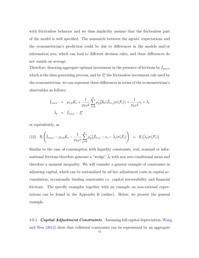
with frictionless behavior and we thus implicitly assume that the frictionless part

of the model is well specified. The mismatch between the agents’ expectations and

the econometrician’s prediction could be due to differences in the models and/or

information sets, which can lead to different decision rules, and these differences do

not vanish on average.Therefore, denoting aggregate optimal investment in the presence of frictions by Icon,t,

which is the data generating process, and by I˚t the frictionless investment rule used by

the econometrician, we can represent these differences in terms of the econometrician’s

observables as follows:

Icon,t “ ρ1,0Kt `1

ρ2,0s

8ÿ

j“0ρ´j2,0EtpZt`j|σpFtqq `

1ρ2,0s

et ` λt

λt “ Icon,t ´ I˚t

or equivalently, as

E

˜

Icon,t ´ ρ1,0Kt ´1

ρ2,0s

8ÿ

j“0ρ´j2,0Zt`j ´ et ´ λt|σpFtq

¸

“ E`

λt|σpFtq˘

(12)

Similar to the case of consumption with liquidity constraints, real, nominal or infor-

mational frictions therefore generate a “wedge” λt with non zero conditional mean and

therefore a moment inequality. We will consider a general example of constraints in

adjusting capital, which can be rationalized by ad hoc adjustment costs in capital ac-

cumulation, occasionally binding constraints i.e. capital irreversibility and financial

frictions. The specific examples together with an example on non-rational expec-

tations can be found in the Appendix B (online). Below, we present the general

example.

3.0.1. Capital Adjustment Constraints. Assuming full capital depreciation, Wang

and Wen (2012) show that collateral constraints can be represented by an aggregate15

function ψpιtq of the investment rate, ιt ” ItKt. Note that this representation can

be rationalized with different setups, including those in which there is a distribution

of investment efficiency shocks across firms. Moreover, such setups can be further

microfounded by different mechanisms i.e. financial frictions à la Bernanke, Gertler,

and Gilchrist (1999). Focusing on exogenous collateral constraints, i.e. the borrowing

limit does not depend on the asset value of the collateral10, they imply the following

subsystem of linearized aggregate equilibrium conditions:

Kt`1 “ ψ1ssIt ` p1´ ψ1ssqKt(13)

Qt “ ´ψ1´1ss ψ

2sspIt ´ Ktq(14)

Qt “ ωCt ´ ωEt ˜Ct`1 `Ψss,1EtRt`1 ` EtQt`1 ` pψ1ss ´ 1qEtpIt`1 ´ Kt`1q(15)

where Ψss,1 ” 1` βpψ1ss ´ 1q.

Denoting by Ψss,2 ” ωpψ1ssspα´ sq` sq´ sp1´ sqψ1´1ss ψ

2ss, γ1 ” Ψ´1

ss,2pωs´ψ1´1ss ψ

2sssp1´

sqq, γ2 ” Ψ´1ss,2ω and γ3 ” Ψ´1

ss,2Ψss,1p1´ sq the first order condition (9) becomes

γ1EtIt`1 ´ p1` γ1 ` p1´ αqγ3qIt ` It´1 “ γ2Zt(16)

whose solution generalizes to:

Icon,t “ ρ1pγqKt `1

ρ2pγqspγqZt `

1ρ2et ` λt

For ρipγ0q ” ρi,0, spγ0q ” s0, the corresponding distortion due to capital adjustment

constraints is equivalent to

λt “ pρ1pγq ´ ρ1pγ0qq Kt `

ˆ

1ρ2pγqspγq

´1

ρ2pγ0qspγ0q

˙

Zt `

ˆ

1ρ2pγq

´1

ρ2pγ0q

˙

et

10Endogenous collateral constraints have a different representation than exogenous constraints. Nev-ertheless, as Wang and Wen (2012) note, endogenous collateral constraints imply a form of aggregateinvestment externality which implies insufficient level of investment relative to the case of exogenousconstraints. This simply reinforces the distortions we derive based on exogenous constraints.

16

In order to determine the sign of E`

λt|σpFtq˘

, it is sufficient to look at the sign of the

coefficient of Kt. Using a mean value expansion around zero, the conditional mean is

E`

λt|σpFtq˘

“ ρ11pγqKt where ρ1pγq1 ” ρ1pγq

1

p´q

pγ1 ´ γ1,0qp`q

` ρ11p`q

pγqpγ3 ´ γ3,0qp´q

ď 0.

Frictions in capital accumulation therefore generate negative endogenous distortions,

which implies that EλtKt ď 011.

The preceding example dealt with distortions in the decision rules, which directly

affect- and are therefore informative for- the transmission of shocks and welfare.

Moreover, they can be easily linked to additional data. Nevertheless, frictions are

always justified using the first order necessary conditions for agents’ optimal deci-

sions. In the next section, we present the general case together with a representation

result, which proves useful in translating distortions to the first order conditions into

observationally equivalent general equilibrium distortions to decision rules. One can

therefore directly use the latter. Because we work with linearized models, second or

higher order effects will be ignored. However, moment inequalities, would also ap-

pear in nonlinear models. The way we treat frictions does not depend on assumptions

regarding the approximation error.

4. Perturbing the Frictionless Model

The general framework involves a system of expectational equations . Denote by xi,t

the endogenous individual state, by zi,t the exogenous individual state, and by Xt “´xi,tdΛpiq and Zt “

´zi,tdΛpiq the corresponding aggregate states. The optimality

11The signs hold uniformly over γ, for any twice differentiable function ψ. This is straightforwardfor the derivatives, while for γi´ γi,0, this gives rise to a quadratic inequality in ψ1ss which holds forall plausible ψ1ss P p0, 1s.

17

conditions characterizing the individual decisions are as follows:

Gpθqxi,t “ F pθqEi,t

¨

˝

¨

˝

xi,t`1

Xt`1

˛

‚|xi,t, zi,t, Xt, Zt

˛

‚` Lpθqzi,t(17)

zi,t “ Rpθqzi,t´1 ` εi,t

where Epεi,tq “ 0. We assume that the coefficients of the behavioural equations

are common across agents. Relaxing this assumption would make the notation more

complicated, but would not change the essence of our argument. We could also specify

equilibrium conditions that involve past endogenous variables but this is unnecessary

as we can always define dummy variables of the form xi,t ” xi,t´1 and enlarge the

vector of endogenous variables to include xi,t. Aggregating across individuals, the

economy can be characterized by the following system:

GpθqXt “ F pθq

ˆEi,t

¨

˝

¨

˝

xi,t`1

Xt`1

˛

‚|xi,t, zi,t, Xt, Zt

˛

‚dΛtpiq ` LpθqZt(18)

Zt “ RpθqZt´1 ` εt(19)

We will refer to the economy with frictions as the triple pHpθq,Λ, Eiq where

Hpθq ” pvecpGpθqT q, vecpF pθqqT , vecpLpθqqT , vecpRpθqqT , vechpΣεqTq.

We partition the vector θ into two subsets, pθ1, θ2q where θ2 collects the parameters

characterizing the presence and intensity of frictions. Thus, setting θ2 “ 0, reduces the

model to the frictionless economy and this is without loss of generality. Furthermore,

in an economy with no frictions, prices efficiently aggregate all the information. Thus18

there is no need to distinguish between individual and aggregate information when

predicting aggregate state variables.

For wi,t ” pxi,t, Xi,t, zi,t, Zi,tq, when agents are rational, and the model is linear ( or

linearized) aggregate expectations for pxTi,t`1, XTt`1q

T become as follows:

Exi,t`1 “

¨xi,t`1pipxi,t`1, Xt`1|wi,tqdpxi,t`1, Xt`1qdΛtpiq

“

¨xi,t`1ppxi,t`1|wi,tqdpxi,t`1qdΛtpiq

“

ˆPi,1xi,tdΛpiq ` P2Xt `

ˆPi,3zi,tdΛtpiq ` P4Zt

EXt`1 “

¨Xt`1pipxi,t`1, Xt`1|wi,tqdpxi,t`1, Xt`1qdΛtpiq

“

ˆXt`1ppXt`1|Xt, ZtqdpXt`1q

“ P5Xt ` P6Zt ” EpXt`1|Xt, Ztq

where Pj,j“1..6 are the coefficients of the linear projection. By Rational expectations

and since the coefficients pG,F, Lq are common across i, equilibrium consistency re-

quires Pi,1 “ P1, Pi,2 “ P2 and therefore P1 ` P2 “ P5 and P3 ` P4 “ P6. Thus,

as expected, aggregate conditional expectations collapse to EpXt`1|Xt, Ztq, and the

frictionless economy, pHpθ1, 0q,Λ,Eq, can be summarized by the equilibrium condi-

tions:

Gpθ1, 0qXt “ F pθ1, 0qEtpXt`1|Xt, Ztq ` Lpθ1, 0qZt(20)

Zt “ RpθqZt´1 ` εt(21)19

Using the decision rule in the expectational system (20) and solving for the undeter-

mined coefficients 12, a Rational Expectations equilibrium for pHpθ1, 0q,Λ,Eq holds

under the following conditions:

. ASSUMPTION-EQ

There exist unique matrices P ˚pθ1, 0qnxˆnx

, Q˚pθ1, 0qnxˆnz

satisfying:

pF pθ1, 0qP ˚pθ1, 0q ´G˚pθ1, 0qqP ˚pθ1, 0q “ 0

pRpθqT b F pθ1, 0q ` Iz b p´F pθ1, 0qP ˚pθ1, 0q `G˚pθ1, 0qqqvecpQpθ1, 0qq “ ´vecpLpθ1, 0qq

such that Xt “ P ˚pθ1, 0qXt´1 `Q˚pθ1, 0qZt is a competitive equilibrium.

Since we know the model up to θ2 “ 0, we rearrange the equations of the economy

with frictions into the known and the unknown part of the specification. Adding and

subtracting the first order conditions of the frictionless economy we get that:

Gpθ1, 0qXt “ F pθ1, 0qEtpXt`1|Xtq ` Lpθ1, 0qZt ` µt(22)

µt ” ´pGpθq ´Gpθ1, 0qqXt ` pLpθq ´ Lpθ1, 0qqZt

`pF pθq ´ F pθ1, 0qqˆ

Eit

¨

˝

¨

˝

xi,t`1

Xt`1

˛

‚|xi,t, Xt

˛

‚dΛtpiq

`F pθ1, 0qpˆ

Eit

¨

˝

¨

˝

xi,t`1

Xt`1

˛

‚|xi,t, Xt

˛

‚dΛtpiq ´ EtpXt`1|Xtqq

This system of equations cannot be solved without knowing µt. Nevertheless, we

characterize the relationship between µt and a set of candidate decision rules that

depend on the endogenous states and some unobserved process, λt. Proposition 1

states sufficient conditions such that decision rules are consistent with µt.

12See for example Marimon and Scott (1998).20

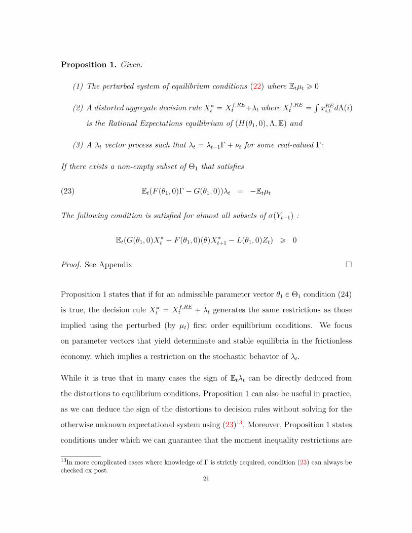
Proposition 1. Given:

(1) The perturbed system of equilibrium conditions (22) where Etµt ě 0

(2) A distorted aggregate decision rule X˚t “ Xf,RE

t `λt where Xf,REt “

´xREi,t dΛpiq

is the Rational Expectations equilibrium of pHpθ1, 0q,Λ,Eq and

(3) A λt vector process such that λt “ λt´1Γ` νt for some real-valued Γ:

If there exists a non-empty subset of Θ1 that satisfies

EtpF pθ1, 0qΓ´Gpθ1, 0qqλt “ ´Etµt(23)

The following condition is satisfied for almost all subsets of σpYt´1q :

EtpGpθ1, 0qX˚t ´ F pθ1, 0qpθqX˚

t`1 ´ Lpθ1, 0qZtq ě 0

Proof. See Appendix

Proposition 1 states that if for an admissible parameter vector θ1 P Θ1 condition (24)

is true, the decision rule X˚t “ Xf,RE

t ` λt generates the same restrictions as those

implied using the perturbed (by µt) first order equilibrium conditions. We focus

on parameter vectors that yield determinate and stable equilibria in the frictionless

economy, which implies a restriction on the stochastic behavior of λt.

While it is true that in many cases the sign of Etλt can be directly deduced from

the distortions to equilibrium conditions, Proposition 1 can also be useful in practice,

as we can deduce the sign of the distortions to decision rules without solving for the

otherwise unknown expectational system using (23)13. Moreover, Proposition 1 states

conditions under which we can guarantee that the moment inequality restrictions are

13In more complicated cases where knowledge of Γ is strictly required, condition (23) can always bechecked ex post.

21

going to be consistent with the rest of the model, and therefore the implied reduced

form.

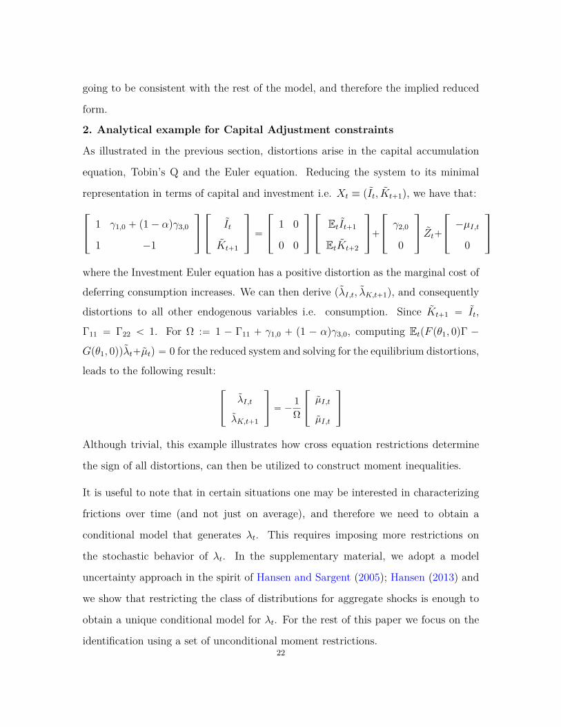
2. Analytical example for Capital Adjustment constraints

As illustrated in the previous section, distortions arise in the capital accumulation

equation, Tobin’s Q and the Euler equation. Reducing the system to its minimal

representation in terms of capital and investment i.e. Xt ” pIt, Kt`1), we have that:»

–

1 γ1,0 ` p1´ αqγ3,0

1 ´1

fi

fl

»

–

It

Kt`1

fi

fl “

»

–

1 0

0 0

fi

fl

»

–

EtIt`1

EtKt`2

fi

fl`

»

–

γ2,0

0

fi

fl Zt`

»

–

´µI,t

0

fi

fl

where the Investment Euler equation has a positive distortion as the marginal cost of

deferring consumption increases. We can then derive pλI,t, λK,t`1q, and consequently

distortions to all other endogenous variables i.e. consumption. Since Kt`1 “ It,

Γ11 “ Γ22 ă 1. For Ω :“ 1 ´ Γ11 ` γ1,0 ` p1 ´ αqγ3,0, computing EtpF pθ1, 0qΓ ´

Gpθ1, 0qqλt`µtq “ 0 for the reduced system and solving for the equilibrium distortions,

leads to the following result:»

–

λI,t

λK,t`1

fi

fl “ ´1Ω

»

–

µI,t

µI,t

fi

fl

Although trivial, this example illustrates how cross equation restrictions determine

the sign of all distortions, can then be utilized to construct moment inequalities.

It is useful to note that in certain situations one may be interested in characterizing

frictions over time (and not just on average), and therefore we need to obtain a

conditional model that generates λt. This requires imposing more restrictions on

the stochastic behavior of λt. In the supplementary material, we adopt a model

uncertainty approach in the spirit of Hansen and Sargent (2005); Hansen (2013) and

we show that restricting the class of distributions for aggregate shocks is enough to

obtain a unique conditional model for λt. For the rest of this paper we focus on the

identification using a set of unconditional moment restrictions.22

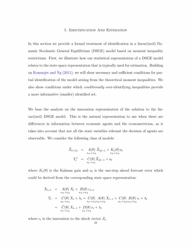
5. Identification And Estimation

In this section we provide a formal treatment of identification in a linear(ized) Dy-

namic Stochastic General Equilibrium (DSGE) model based on moment inequality

restrictions. First, we illustrate how our statistical representation of a DSGE model

relates to the state space representation that is typically used for estimation. Building

on Komunjer and Ng (2011), we will show necessary and sufficient conditions for par-

tial identification of the model arising from the theoretical moment inequalities. We

also show conditions under which conditionally over-identifying inequalities provide

a more informative (smaller) identified set.

We base the analysis on the innovation representation of the solution to the lin-

ear(ized) DSGE model. This is the natural representation to use when there are

differences in information between economic agents and the econometrician, as it

takes into account that not all the state variables relevant the decision of agents are

observable. We consider the following class of models:

Xt`1|t “ ApθqnXˆnX

Xt|t´1 ` KtpθqnXˆnX

at

Y ot “ Cpθq

nY ˆnx

Xt|t´1 ` at

where Ktpθq is the Kalman gain and at is the one-step ahead forecast error which

could be derived from the corresponding state space representation:

Xt`1 “ ApθqnXˆnX

Xt ` BpθqnXˆnX

εt`1

Yt “ CpθqnY ˆnX

Xt ` λt “ CpθqnY ˆnX

ApθqnXˆnX

Xt´1 ` CpθqnY ˆnX

BpθqnXˆnX

εt ` λt

“ CpθqnY ˆnX

Xt´1 ` DpθqnY ˆnX

εt ` λt

where εt is the innovation to the shock vector Zt.23

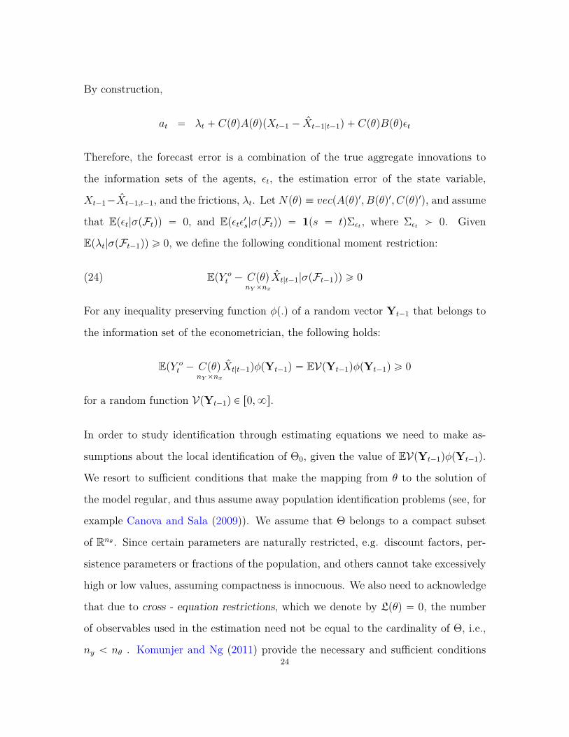
By construction,

at “ λt ` CpθqApθqpXt´1 ´ Xt´1|t´1q ` CpθqBpθqεt

Therefore, the forecast error is a combination of the true aggregate innovations to

the information sets of the agents, εt, the estimation error of the state variable,

Xt´1´Xt´1,t´1, and the frictions, λt. Let Npθq ” vecpApθq1, Bpθq1, Cpθq1q, and assume

that Epεt|σpFtqq “ 0, and Epεtε1s|σpFtqq “ 1ps “ tqΣεt , where Σεt ą 0. Given

Epλt|σpFt´1qq ě 0, we define the following conditional moment restriction:

(24) EpY ot ´ Cpθq

nY ˆnx

Xt|t´1|σpFt´1qq ě 0

For any inequality preserving function φp.q of a random vector Yt´1 that belongs to

the information set of the econometrician, the following holds:

EpY ot ´ Cpθq

nY ˆnx

Xt|t´1qφpYt´1q “ EVpYt´1qφpYt´1q ě 0

for a random function VpYt´1q P r0,8s.

In order to study identification through estimating equations we need to make as-

sumptions about the local identification of Θ0, given the value of EV(Yt´1)φ(Yt´1).

We resort to sufficient conditions that make the mapping from θ to the solution of

the model regular, and thus assume away population identification problems (see, for

example Canova and Sala (2009)). We assume that Θ belongs to a compact subset

of Rnθ . Since certain parameters are naturally restricted, e.g. discount factors, per-

sistence parameters or fractions of the population, and others cannot take excessively

high or low values, assuming compactness is innocuous. We also need to acknowledge

that due to cross - equation restrictions, which we denote by Lpθq “ 0, the number

of observables used in the estimation need not be equal to the cardinality of Θ, i.e.,

ny ă nθ . Komunjer and Ng (2011) provide the necessary and sufficient conditions24

for local identification of the DSGE model from the auto-covariances of the data. We

reproduce them below, with the minor modification that Assumption LCI-6 holds

for any element of the identified set Θ0.

. ASSUMPTION -LCI (Local Conditional Identification)

(1) Θ is compact and connected

(2) (Stability) For any θ P Θ and for any z P C, detpzInX ´ Apθqq “ 0, implies

|z| ă 1

(3) For any θ P Θ, DpθqΣeDpθq1 is non-singular

(4) For any θ P Θ, (i) The matrix pKpθqApθqKpθq .., ApθqnX´1Kpθqq has full row

rank and pCpθq1Apθq1Cpθq1 .., Apθq1nX´1Cpθq1q1 has full column rank.

(5) For any θ P Θ, the mapping N : θ ÞÑ Npθq is continuously differentiable

(6) Rank of ∆NSpθq 14 is constant in a neighborhood of θ0 P ΘI and is equal to

nθ ` n2x

Lemma 3. Given Vip.q P rVp.q, Vp.qs, and Assumption LCI, θ is locally conditionally

identified at any θ0 in ΘI from the auto-covariances of Yt.

Proof. See Appendix

Given the maintained assumptions, we next characterize the identified set implied by

the restrictions using macroeconomic data.

14 For δNSpθ, T q “ pvecpTApθqT´1qT , vecpTKpθqqT , vecpCpθqT´1qT , vechpΣαpθqqT qT ,

∆NSpθ0q “ pBδNSpθ,Inx q

Bθ , BδNSpθ,Inx qBvecT q|θ“θ0

25

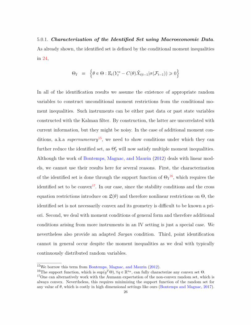
5.0.1. Characterization of the Identified Set using Macroeconomic Data.

As already shown, the identified set is defined by the conditional moment inequalities

in 24,

ΘI ”

!

θ P Θ : EtpY ot ´ CpθqXt|t´1|σpFt´1qq ě 0

)

In all of the identification results we assume the existence of appropriate random

variables to construct unconditional moment restrictions from the conditional mo-

ment inequalities. Such instruments can be either past data or past state variables

constructed with the Kalman filter. By construction, the latter are uncorrelated with

current information, but they might be noisy. In the case of additional moment con-

ditions, a.k.a supernumerary15, we need to show conditions under which they can

further reduce the identified set, as Θ1I will now satisfy multiple moment inequalities.

Although the work of Bontemps, Magnac, and Maurin (2012) deals with linear mod-

els, we cannot use their results here for several reasons. First, the characterization

of the identified set is done through the support function of ΘI16, which requires the

identified set to be convex17. In our case, since the stability conditions and the cross

equation restrictions introduce on Lpθq and therefore nonlinear restrictions on Θ, the

identified set is not necessarily convex and its geometry is difficult to be known a pri-

ori. Second, we deal with moment conditions of general form and therefore additional

conditions arising from more instruments in an IV setting is just a special case. We

nevertheless also provide an adapted Sargan condition. Third, point identification

cannot in general occur despite the moment inequalities as we deal with typically

continuously distributed random variables.

15We borrow this term from Bontemps, Magnac, and Maurin (2012).16The support function, which is suppqT Θq,@q P Rnθ , can fully characterize any convex set Θ.17One can alternatively work with the Aumann expectation of the non-convex random set, which isalways convex. Nevertheless, this requires minimizing the support function of the random set forany value of θ, which is costly in high dimensional settings like ours (Bontemps and Magnac, 2017).

26

Recall that the number of moment conditions we use for estimation depend on the

number of observables. Assumption LCI-6 requires that there has to be enough (or

the right kind) of observables such that a rank condition is satisfied. In our case, the

number of observables used determines the number of first order conditions used for

estimation. The minimum number (r) of observables required such that conditional

identification is achieved ( Lemma 4 is satisfied) maps to the necessary first order

conditions. For example, if we have Y1 and Y2 to estimate the model, and we only

need Y1 to conditionally identify θ, then the nθ ˆ 1 first order conditions arising from

Y1 will be the necessary conditions. The rest of the conditions, i.e. those arising from

Y2 are then supernumerary.

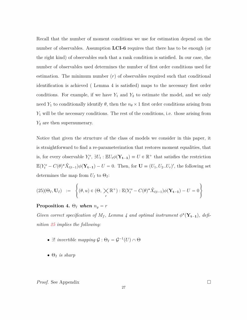
Notice that given the structure of the class of models we consider in this paper, it

is straightforward to find a re-parameterization that restores moment equalities, that

is, for every observable Y ot , DUt : EUtφpYt´1q ” U P R` that satisfies the restriction

EpY ot ´ Cpθq˚Xt|t´1qφpYt´1q ´ U “ 0. Then, for U ” pU1, U2..Urq

1, the following set

determines the map from UI to ΘI :

pΘI ,UIq :“#

pθ, uq P pΘ,ą

r

R`q : EpY ot ´ Cpθq

˚Xt|t´1qφpYt´1q ´ U “ 0+

(25)

Proposition 4. ΘI when ny “ r

Given correct specification of Mf , Lemma 4 and optimal instrument φ˚pYt´1q, defi-

nition 25 implies the following:

‚ D! invertible mapping G : ΘI “ G´1pUq XΘ

‚ ΘI is sharp

Proof. See Appendix 27

Note that the proposition applies to the infeasible case of using optimal instruments.

If the case of non-optimal but valid instruments, the set is again as sharp as possible,

up to the information loss implied by the non-optimality of the instrument18. It is also

important to note that our characterization is based on the fact that the unobserved

endogenous variables are integrated out using the Kalman filter. This implies that the

only unobservables we need to deal with in the characterization of ΘI is the aggregate

shocks in the economy. Moreover, the set is robust to individual heterogeneity as long

as it vanishes on aggregate. More importantly, given correct specification, U is non

zero if and only if there is a positive mass of agents that indeed face frictions.

Having established the determination of ΘI using the minimum number of observ-

ables, we turn to the case of using a larger number of observables, including non-

macroeconomic variables. Let mα,tpθq and mβ,tpθq denote the necessary and super-

numerary moment functions for identifying Θ, where Epmα,tpθq|Yt´1q “ VαpYt´1q P

rVαpYt´1q, VαpYt´1qq and Epmβ,tpθq|Yt´1q “ VβpYt´1q P rVβpYt´1q, VβpYt´1qq. For

notational brevity, we drop the dependence on Yt´1 hereafter.

Comparing these general bounds to the ones implied by the model equilibrium re-

strictions, Vα “ Vβ “ 0 and Vα “ Vβ “ 8. Due to the boundedness of Θ and

the cross-equation and stability restrictions, the effective lower and upper bounds are

likely to lie strictly within r0,8q for every moment condition. Let φp.q be any Yt´1´

measurable function for which mα,tpθq :“ mα,tpθqφt and mβ,tpθq :“ mβ,tpθqφt, mαpθq

and mβpθq the corresponding vectors, and mαpθq and mβpθq the vector means.

Let W be a real valued, possibly random weighting matrix, diagonal in pWα,Wβq.

Furthermore, denote by Qα the conditional expectation operator when conditioning

on W12Tα mαpθq and by QKα the residual.

18Recent work in the literature proposes constructing instrument functions to avoid this informationloss, see for example Andrews and Shi (2013). We nevertheless do not pursue this in this paper.

28

The following proposition specifies the additional restrictions that need to be satisfied

by the additional moment conditions such that the size of the identified set becomes

smaller. This is a general result, and it applies both to conventional cases where

nY ą r or when data on non-macroeconomic variables is used.

Proposition 5. The Identified Set with Multiple Conditions Given

(1) ΘI ‰ H

(2) Ut P rU, U s, with U ” pW12Tα Vα `W

12Tβ Vβqφt, U ” pW

12Tα Vαt `W

12Tβ Vβqφt

Then Θ1I Ă ΘI iff

(26) EQKα´

W12Tβ mβ,tpθq ´ Ut

¯

“ 0

Proof. See the Appendix

The main argument behind Proposition 5 is the following. Suppose that the necessary

moment conditions have no common information with the supernumerary conditions

and that W “ Inα`nβ . From the minimization of E12pm ´ Utq

T pmpθq ´ Utq where

mpθq ” pmαpθq, mβpθqqT , the first order condition is

Epmαpθq ` mβpθq ´ Utq “ 0

which for Uα ” QKαUt can be rewritten as Eppmαpθq ´ Uαq ` pmβpθq ´ UKα qq “ 0. By

construction the two parts of the left hand side of the expression are independent,

and therefore both have to be zero.

Epmαpθq ´ Uαq “ 0(27)

Epmβpθq ´ UKα q “ 0(28)

29

Notice that, by construction, the set of necessary moment conditions in 5.3. must

have full rank, and this establishes a one-to-one mapping from Θ to the domain of

variation of Ut, rUpYt´1q, UpYt´1qs. Thus, there exists an inverse operator Gα such

that θ “ GαpUt,Pq. Plugging this expression for θ in 5.4, we get that

EmβpGαpUt,Pqq “ EUKα

This is a restriction on the values that Ut can take in addition to the ones implied by

the necessary conditions. A restriction on Ut implies a restriction on the admissible

ΘI given the one-to-one relationship in 5.3. Notice that when the supernumerary con-

ditions do not add any additional information, i.e. mα,tpθq ” mβ,tpθq, the restriction

collapses to Qα “ QKα “12 . Given these identification results, we can analyze identi-

fication arising from any inequality restriction, and therefore any additional type of

information can be potentially analyzed. Below, we discuss and formally show how

qualitative survey data can provide additional restrictions that are informative about

aggregative models of economies with frictions. Such information constrains further

the stochastic properties of λt, and therefore the size of ΘI .

6. The use of additional information

Additional data can be potentially linked to dynamic equilibrium models by augment-

ing the observation equation with moment restrictions. The latter can be motivated

by the fact that not all data are explicitly modeled using structural equations, but

they can nevertheless be used to sharpen economic and econometric inference, espe-

cially for unobserved processes. An example of such a process is the distortion λt. We

focus on qualitative survey data because, as we illustrate, they contain distributional

information that can be linked to the aggregate model and are informative about λt.

This is especially true for economies with frictions, as the proportion of agents whose30

behavior is distorted is an important statistic. An example of a distributional statistic

that has been routinely used to judge the validity of complete models is the propor-

tion of firms which cannot change prices in New Keynesian models featuring a Calvo

adjustment mechanism. Our focus is on more general information that is contained in

qualitative surveys, and given that we deal with incomplete models, this information

is able to discard a set of economic mechanisms, and not just one. We thus view our

method as a significant generalization of the treatment of microeconomic information

in dynamic equilibrium models.

Qualitative survey data are usually available in the form of aggregate statistics, where

aggregation is performed over categories of answers to particular questions. As in

micro-econometric studies, the categorical variable is a function of a continuous latent

variable. In a structural context, there is a measurable mapping from the categories

of answers to the random variables relevant to the decision of each agent. For ex-

ample, if the question is of the type "How do you expect your financial situation to

change over the next quarter" and the answer is trichotomous, i.e "Better", "Same"

and "Worse", then the answers map to a set of partitions of the end of period as-

sets at`2: at`2 P rat`1 ´ ε,8q, at`2 P pat`1 ´ ε, at`1 ` εq and at`2 P p´8, at`1 ´ εs.

For this interpretation to hold, we need to assume that agents report their states

or beliefs truthfully. Furthermore, denote by tSi,k,tuiďN the survey sample over a

period of length T, for the ith respondent. Let Ckl be the lth categorical answer to

question k and ξi,t,k the respondent’s choice. Given some weights on each category

wl, the available statistics are of the form: Bkt “

ř

lďLwlř

iďN 1pξi,t P Ckq. Given

truth telling, we can map the answer to agent beliefs i.e. there exists a mapping

h : ξi,t Ñ ξi,t ” Ei,tpxi,t`1|xi,t, Xtq. Moreover, since the conditional expectation is a

function of the information set, let Bl ” tpxi,t, Xtq P R2nx : hpxi,t, Xtq P Ckl u, that

is, Bl belongs to the partition of the support of individual xi,t (or aggregate Xtq31

that corresponds to category Ckl . Consequently, the survey statistic has the following

theoretical form, which can be linked to the model:

Bkt “

ÿ

lďL

wlÿ

iďN

wi1pEi,tpxt`1,i|xi,t, Xtq P Blq(29)

For every Y ot with a corresponding model based conditional expectation Y m

t ” EpY ot |M,Ftq,

Proposition 6 illustrates the additional restrictions implied by Bkt . For these to hold,

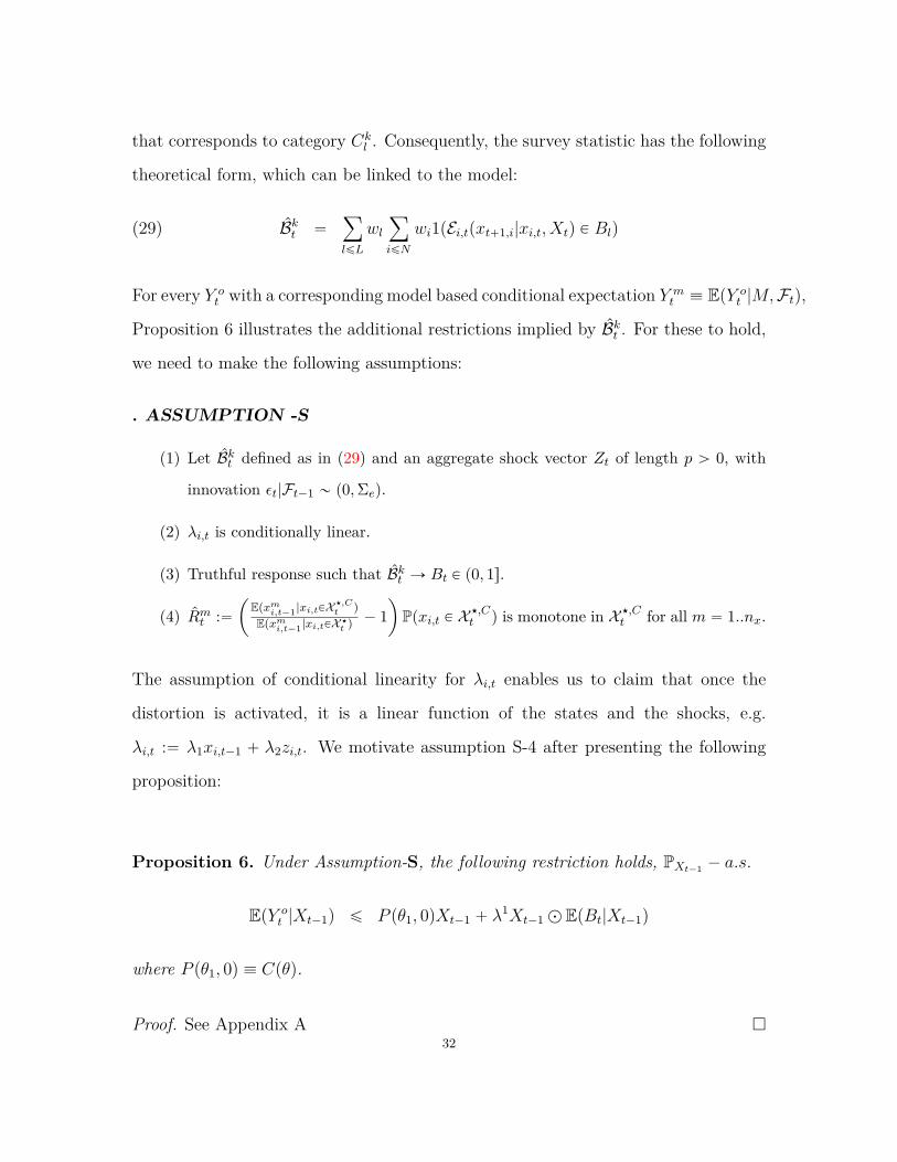
we need to make the following assumptions:

. ASSUMPTION -S

(1) Let Bkt defined as in (29) and an aggregate shock vector Zt of length p ą 0, with

innovation εt|Ft´1 „ p0,Σeq.

(2) λi,t is conditionally linear.

(3) Truthful response such that Bkt Ñ Bt P p0, 1s.

(4) Rmt :“ˆ

Epxmi,t´1|xi,tPX ‹,Ct q

Epxmi,t´1|xi,tPX ‹t q´ 1

˙

Ppxi,t P X ‹,Ct q is monotone in X ‹,C

t for all m “ 1..nx.

The assumption of conditional linearity for λi,t enables us to claim that once the

distortion is activated, it is a linear function of the states and the shocks, e.g.

λi,t :“ λ1xi,t´1 ` λ2zi,t. We motivate assumption S-4 after presenting the following

proposition:

Proposition 6. Under Assumption-S, the following restriction holds, PXt´1 ´ a.s.

EpY ot |Xt´1q ď P pθ1, 0qXt´1 ` λ

1Xt´1 d EpBt|Xt´1q

where P pθ1, 0q ” Cpθq.

Proof. See Appendix A 32

Notice that in the proof, we define pX ‹t ,Z‹

t q as the time dependent subset of the

support such that λi,t ‰ 0. In models of heterogeneous agents these boundaries

usually depend on aggregate states and shocks. Therefore, this inequality will in

general be strict unless Bt “ 0.

Moreover, in the proof we establish two facts. First, since the equilibrium conditions

of the model with frictions depend on subjective conditional expectations, and the

model with frictions is a smooth perturbation of the frictionless model, any probability

statement on the subjective expectations translates to a probability statement on

µi,t. Second, any probability statement on µi,t is a probability statement on the

solution of the model, and therefore on λi,t. Given representation (29), qualitative

survey data have information on the quantiles of subjective conditional expectations

of the agents. Therefore, survey data relate directly to the conditional probability

of observing a friction, Ptpλi,t ě 0q, which implies the above restrictions. The latter

cannot in general deliver point identification, as the vector Rt “ pR1t , R

2t ...R

nxt q is

hard to pin down unless specific assumptions are made. Monotonicity, which is a

mild assumption, provides a bound.

Given Proposition 6, we can also establish the following corollary result regarding

identification using survey data.

Corollary 7. Identification with Survey Data

(1) If Bkt Ñ Bt P p0, 1q, Θ1

I Ă ΘI .

(2) Impossibility of point identification: When Bt ‰ 0, ΘI is not a singleton

Proof. See Appendix

Corollary 7 has several implications. First, the set of admissible structures becomes

smaller, and we can therefore make more precise statements regarding parameters and33

conditional predictions. Second, using identified set and the definition of λpYt, θq, a

plug-in set estimate of the average distortion (wedge) in a macroeconomic variable Yt

is EλpYt, θIpY qq. These estimates of distortions can be used in several ways, which

we explore in the next section.

7. Inference based on λpΘIq

We first discuss briefly how ΘI and λpΘIq can be obtained in practice. Given the

quasi-structural framework, performing inference for ΘI rather than θ0 seems a natu-

ral thing to do. Many of the parameters in dynamic macroeconomic models are semi-

structural, and therefore θ0 itself does not have a very specific economic interpretation.

We therefore use methods appropriate for constructing consistent estimators for the

identified set (IdS) and confidence sets (CS) for the IdS. In the frequentist literature,

several methods have been proposed for a general criterion function like subsampling

Chernozhukov, Hong, and Tamer (2007); Romano and Shaikh (2010) or the bootstrap

for moment inequality models Bugni (2010). Nevertheless, in macroeconomic models

parameter dimensions are high and pointwise testing is a vastly inefficient way to con-

struct confidence sets, so we focus on computationally tractable methods to perform

statistical inference using Markov Chain Monte Carlo algorithms (MCMC).

When θ0 is point identified and root-n estimable, Chernozhukov and Hong (2003) have

proposed to use simulation methods to do inference on θ using the quasi-posterior

distribution, which is constructed using the relevant loss function Lnpθq that defines

θ0. Generalized Method of Moment (GMM) class of estimators can be easily embed-

ded in this case. Denoting by πpθq the prior distribution, simulation draws tθjujďLare obtained from

Πnpθ|Yq ”exppTLnpθqq´

Θ exp pTLnpθqqdπpθq34

and upper and lower 100p1 ´ αq2 quantiles are used to conduct inference that has

valid frequentist properties. Nevertheless, once point identification fails, one has to

consider adjusting the method to accommodate for this.

More particularly, let Lnpθq “ n12 qnpθq

1`Wnn

12 qnpθq` be the criterion function to

be minimized, where qnpθq are the moment functions to be used and qnpθq` ”

maxpqnpθq, 0q “ minp´qnpθq, 0q. If Lnpθq is stochastically equicontinuous, that is,

there exists a ∆npθ0q and Jnpθ0q such that Lnpθq admits a quadratic expansion 19

then this allows us to assume a Central Limit Theorem (CLT) on ∆npθ0q. Redefining

Qnpθq ” qnpθq ´ b where b is the bias term and Lnpθ, bq “ n12Qnpθq

1Wnn12Qnpθq, we

assume that the following CLT holds

V pθ0, b0q´ 1

2 ∆npθ0, b0qdÑ Np0, Iq(30)

Estimating equations arising in DSGE models involve smooth functions. This isparticularly true if we focus on determinate equilibria, so that model specification

is uniform across the parameter space. Combining them with smooth instrument

functions is enough to guarantee stochastic equicontinuity.

Given 30, Liao and Jiang (2010) show that when using a cutoff rate νn such that 1 ă

νn ă n, and defining An :“ tmaxϑ lnpΠnpϑ|Yqq ´ lnpΠnpθ|Yqq ď νnu then dHpAn,ΘIq Ñp

0 where dHp., .q is the Hausdorff distance between two sets 20. Moreover, the rate of

convergence of the pseudo-posterior density outside the identified region is exponen-

tial. As is evident, in finite samples the identified will depend on νn, so some ro-

bustness checks are required. In addition, since our criterion function vanishes when

19

Lnpθq “ Lnpθ0q` pθ ´ θ0q1∆npθ0q ´

12 pθ ´ θ0q

1nJnpθ0qpθ ´ θ0q `Rnpθq

20dHp., .q “ max rsupaPA infbPB ||b´ a||, supbPB infaPA ||a´ b||s35

θ P ΘI , we do not need to adjust νn as suggested in Chernozhukov, Hong, and Tamer

(2007).

With regards to constructing confidence sets for the identified set, which is what

we do in the empirical application, recent work by Chen, Christensen, O’Hara, and

Tamer (2016) provides a computationally attractive procedure to construct ΘCSα for

the IdS and functions of it that have correct coverage from a frequentist perspective.

Compared to Chernozhukov and Hong (2003); Liao and Jiang (2010), cutoff values

are based on quantiles of draws of the loss function Lnpθq rather than draws from the

quasi-posterior of the parameter vector and there is no maximization involved. Also,

results extend to models with singularities, that is models in which a local quadratic

approximation involves a non vanishing singular component, and parameters are not

root-n estimable. This is useful in case one wants to derive bounds based on extensions

to non-parametric treatments of the survey based bounds. Although we find the

method suggested very appealing, we apply it only in the case of estimating frictions.

Proving validity for the testing procedure we will propose in this section is not trivial

as it involves combining two independent MCMC chains, and we leave this interesting

research for the immediate future.

We next motivate the proposed test that utilizes λY pΘIq. When a complete model

is estimated, the pseudo true vector θ0 is point identified. Given its value, we can

estimate the predicted level of friction in each of the macroeconomic variable, EλY pθ0q.

Misspecification of this model may imply that the predicted friction does not lie in

the identified set of distortions. Therefore, the distance from EλY pΘIq becomes a

sufficient statistic to judge whether the suggested model is properly specified. We

propose a Wald statistic that tests whether the expected distance from the point

estimate for the wedge from the parametric model to the identified set of wedges is

different than zero for all (or some of) the observables. Since survey data provide36

more information on the wedge, this increases power to reject non-local alternatives.

In addition, survey data regularizes the test, as in the absence of additional data the

distribution degenerates and requires non-standard inference.

7.0.1. A Test for Parametric Models of Frictions. Letting H0 : θp P Θs and

H1 : θp R Θs, the proposed statistic is as follows:

Wt “

˜

?T infλsPλpΘsq

||V´12 pλs ´ λ

‹pq||

¸2

where λ is the estimated friction obtained using either the identified point in the

parametric model case, λp, or the identified set in the robust case, λs. Individual

frictions are weighted by their respective estimate of standard deviation. The statistic

measures the Euclidean distance between the wedge that arises in the parametric

model, and the set of admissible wedges, adjusted for estimation uncertainty. Under

the following conditions, the test is consistent and has asymptotic power equal to one

against fixed alternatives.

. ASSUMPTION -R (Regularity conditions) Let D and q be Y´ measurable

functions, continuous in θ w.p.1 and qp.; θq ” qp.; θq ´ qp.; θq such that:

(1) For any Y, and any θ P Θ,?T qpY; θq Ñd N p0,Ωq

(2) supθPΘDnpθq Ñp D where D is positive definite

Proposition 8. Consistency and Power. Under assumption R:

(1) TWpθp,ΘsqdÑ ||

ř

j“1..p ωjN p0, Ipq||2

(2) Given critical value cα with α P p0, 1q,

(a) Under H0: limTÑ8

PpTWpθp,Θsq ď cαq “ 1´ α

(b) Under H1: limTÑ8

PpTWpθp,Θsq ď cαq “ 0

Proof. See Appendix 37

In the supplemental material we show that using the non-parametric block bootstrap

to compute cα is valid, and we illustrate through a measurement error example that

the bootstrap distribution coincides with the asymptotic distribution. Thorough ex-

amination of the performance of this test in small samples is a very interesting avenue

of research, which deserves separate treatment. Another equally interesting topic for

future research is to investigate which criterion function would deliver robustness of

the testing procedure to possible misspecification of the benchmark model, which we

have assumed away. See Ponomareva and Tamer (2011) for the issue of misspecifica-

tion in moment inequality models.

Finally, we briefly discuss the refutability of the candidate model, in the sense of

Breusch (1986). The Null hypothesis, tests whether the point identifying restrictions

on λY implied by the candidate model are satisfied on λY,s, where the latter is only set

identified. Since pλY,s, λY,pq is constructed using θ1 as identified using the frictionless

and complete model respectively (See Proposition 1 for the definition of θ1), λY,p is

a function of the additional parameters indexing the CM, θ2. In the absence of cross

parameter (equation) restrictions on Θ1 ˆ Θ2, λY,p would necessarily lie within λY,s

as the latter would be consistent with any θ2 P Θ2. However, in the presence of cross

equation restrictions, pθ1, θ2q lie in a strict subset of Θ1ˆΘ2. Thus, the completion λY,p

may not necessarily lie within the family of completions, λY,s. Equivalently, Dλ P λs

that is not observationally equivalent to λp. In this sense, the candidate model is

refutable only when it imposes restrictions on λy :“ Uypθ1, θ2q for any observable Y ,

which implies restrictions on the reduced form. This is indeed true in the context

of incomplete general equilibrium models; taking the unconditional expectation in

condition (23) of Proposition 1, implies that (Θ1,Θ2) is not variation free and therefore

Uypθ1, θ2q is restricted.38

8. Application: Estimating Frictions in the Spanish Economy

We apply the methodology to the case of Spain, where financial frictions have arguably

played a significant role during the last decade. The benchmark economy we use

features some frictions and since it is standard, we will directly introduce the log-

linearized conditions. We consider a small open economy with capital accumulation,

along the lines of Smets and Wouters (2007) and Gali and Monacelli (2005). There

are households, intermediate good firms, final good firms, government expenditure,

and a foreign sector which is composed by infinitesimal symmetric economies.

The type of frictions we allow in the baseline model are those we do not have suffi-

ciently informative survey data to implement our methodology. Thus, we keep the

parametric Calvo type of friction in the wage setting by labor unions and in the price

setting behavior of firms. All other frictions are going to be semi-parametrically char-

acterized. We thus remove capital adjustment costs, and therefore Tobin’s q becomes

constant. This implies that the arbitrage condition between capital and bonds has

no dynamics in the benchmark model.

Let Xo1 denote the vector of variables that enter the moment equalities, Xo

2 the vec-

tor of variables used in the moment inequalities and Z the vector of instruments.

Model predictions are denoted with superscript ’m’. The conditions we use are there-

fore:

EppXo1,t ´X

m1,tq b Ztq “ 0

EppXo2,t ´X

m2,tq b Ztq ď 0

The variables employed in estimation are Non Government Consumption expenditure

(C), Hours (H), Inflation (π), Investment (I), Gross Domestic Product (Y), Wages

(W), and the EONIA rate (R). Real variables are in per capita terms.We use lagged39

values of output, consumption and investment as instruments, as all positively depend

on the capital stock which is unobserved. We estimate the model using business

survey data from Spain, collected by the European Commission. Our sample period

covers 1999Q1 to 2013Q4. Detailed information on this survey data can be found

at: http://ec.europa.eu/economy_finance/db_indicators/surveys/index_en.

htm. We include responses to questions 8F4 and 8F6, relating to capital adjustment

costs and financial constraints to production capacity. To isolate the effects of using

just the firm survey data, we do not use the consumer survey.

For the case of capital adjustment costs, we have restrictions on Y and I similar

to those of the general example in Section 3. Financial constraints to productive

capacity imply similar restrictions and lead to lower aggregate investment and output.

Although we do not use the consumer survey, we also allow for consumer credit

constraints. The later imply negative distortions to household consumption, and

given that hours worked are complementary to consumption, they also imply negative

distortions to labor supply and output.

We therefore choose Xo1,t ” pW,π,Rq and Xo

2,t ” pY, I,H,Cq. We estimate the model

using the 2-block RW-MCMC with uniform priors for all parameters21. Since the

survey based moment restrictions require estimating the nuisance parameters λ1 (see

Proposition 6), for a given draw of Θ1, we obtain λ1 by ordinary least squares. This

approximation can, in theory, weaken the informativeness of the additional restric-

tions but we do not observe this in our results.

8.1. Details of the exercise. We obtain the 95% confidence sets of wedges, that

is, a range for the standardized wedge in each observable that is consistent with

both macroeconomic and survey data, λy ” pEVy|xEVxq´1EXt,t´1pYt´CpΘIqq, which

21We keep the last 200000-300000 draws for inference.40

under linearity is equivalent to pEVy|xq´1λy

22. These estimates are the empirically

relevant wedges that any model featuring financial frictions and adjustment costs

should produce over the whole sample. We plot them (in red) in the left panel of

Figures 1-4, in Appendix A.

We employ a complete model (CM) featuring Bernanke, Gertler, and Gilchrist (1999)

(BGG) type of frictions (similar to Graeve (2008)) and estimate it using the same

macroeconomic aggregates as the IM using full information MCMC, where we also

rely on Chen, Christensen, O’Hara, and Tamer (2016) to obtain ΘCSα,CM .

Despite that the model features financial frictions on the firm side (the "entrepreneurial

sector"), and not borrowing constrained consumers, its implications can still be tested

against the incomplete model (IM), which is robust to both types of frictions.

We plot (in blue) the corresponding confidence sets for the wedges that are consistent

with the complete model. To facilitate the comparison, we also produce an alternative

comparison based on QQ plots, which gives information on the support of each of these

estimates. Note that in some of the cases the support is completely different.

In Table 1 (Appendix A), we display the corresponding confidence sets for Θ using

survey data. Confidence sets for ΘIM without using survey data and the correspond-

ing wedges can be found in Appendix B.

A key observation is the fact that the sign of the wedge confidence sets that correspond

to the restrictions imposed to identify the IM are in accordance with the sign of the

distortions identified with the CM. While both the CM and IM identify negative

distortions to output, the former identifies a significantly lower level of distortions.

As is typical, empirical versions of accelerator type of models ignore the output costs

22We actually compute λt using quadratic programming as in the second section of the online Ap-pendix (page 70 of this script) and then take the average. The result is equivalent to a standardizedwedge.

41

(bankruptcy costs) as they are deemed to be numerically unimportant. Some of

the neglected variation is indeed captured by the high estimates of φp,CM relative to

φp,IM .

Regarding inflation, using the CM we cannot reject zero frictions to πt, while the

IM identifies significantly negative distortions. Moreover, the CM identifies a much

higher slope of the Phillips curve23, which is consistent with its "inability" to generate

negative distortions to inflation.

With regard to the nominal interest rate, both the CM and the IM identify negative

distortions (with no evidence of different magnitudes). Mechanically, this is due to

the Taylor rule that pins down rt. Nevertheless, there is also a deeper insight which

comes from steady state reasoning. In an economy with uninsured idiosyncratic risk

on both firms and consumers, the steady state interest rate is lower than in the case

of complete markets, and as shown by Angeletos (2007), this does not contradict neg-

ative distortions to capital accumulation due to the presence of a risk premium.

Furthermore, we cannot reject the hypothesis that the CM is consistent with zero

distortions to ct, while the IM identifies negative distortions. Moreover, the estimates

of risk aversion are much lower in the IM compared to the CM. One of the reasons is

the fact that the CM ignores credit constraints to consumers, and therefore requires

much higher estimates in risk aversion to match the corresponding negative distortions

to consumption.

With regard to hours worked, both the IM and the CM identify negative distortions

which are statistically different. Since σc,IM is much smaller than σc,CM , negative

distortions to consumption are consistent with less distortions to hours in the IM.

Moreover, the CM identifies a slightly higher (inverse) Frisch elasticity (σl,CM) and

23κ :“ p1´ιpξpqp1´ξpqp1`βιpqpξpp1`pφc´1qεpqq where εp (Kimball aggregator) is calibrated to 10.

42

does not reject zero distortions to wt, while the IM identifies positive distortions.

The latter observation is not robust to excluding the survey data as shown in Table

2.

Finally, the IM and CM identify the same negative distortions to investment. Since no

marginal Θcs has an extremely narrow support, this result can be possibly explained

by the mapping from parameters to investment that is nearly not injective. This is

not a problem per se, as the MCMC method we have used to obtain confidence sets

in both the IM and the CM is robust to lack of identification.

The non overlapping standardized output, inflation and labour wedges provide enough

evidence to reject the hypothesis that the SW-BGG model implies similar distortions

to those identified by the IM. This finding also corroborates existing evidence of the

lack of uniform fit for such a model over the entire business cycle (i.e. Del Negro,

B. Hasegawa, and Schorfheide (2016) for the case of the US).

9. Conclusion

In this paper we propose a new inferential methodology which is robust to misspeci-

fication of the mechanism generating frictions in dynamic stochastic economies. We

characterize wedges in equilibrium decision rules in a way which is consistent with a

variety of generating mechanisms. We use the implied restrictions to partially identify

the parameters of the benchmark model, and to obtain a set of admissible economic

relationships. Moreover, we formally characterize set identification given the num-

ber of observables. Regarding the latter, beyond macroeconomic data, we show how

qualitative survey data can provide additional distributional information, which is

crucial in economies with ex post heterogeneous and frictions. Survey data provide a

sufficient statistic for this information that would otherwise have to be generated by

a model. We show how to exploit this additional information to test parametrically43

specified models of frictions. We apply our methodology to estimate the distortions

in the Spanish economy due to financial frictions and adjustment costs using an small

open economy version of Smets and Wouters (2007) model and qualitative survey data

collected by the European Commission. We investigate the adequacy of Bernanke,

Gertler, and Gilchrist (1999) type of financial frictions.

In general, our work shows that adopting a robust approach to inference and using

the information present in surveys is a fruitful way of dealing with lack of knowledge

about the exact mechanisms generating frictions.

Our work is limited to dynamic linear economies and has focused on deviations of the

representative agent approximation from the underlying heterogeneous agent econ-

omy. Possible extensions could study deviations based on a benchmark heterogeneous

model. Buera and Moll (2015) have recently shown that the distortions generated in

an aggregate equilibrium condition can depend on the type of heterogeneity present

in the economy. Our approach is robust to this criticism. The methodology does not

rest on observing residuals from representative agent frictionless economies - we just

impose moment inequality restrictions theoretically motivated by deviations from the

frictionless economy. In addition, if heterogeneity has additional implications for the

form of these restrictions, they can be taken on board. In addition, we impose weak

moment inequalities. This is important when heterogeneous distortions in decision

rules cancel out. Furthermore, we impose restrictions implied by µt on all of the

variables and thus take general equilibrium effects into account. Nevertheless, future

work could focus on investigating the robustness of our methodology in environments

where some heterogeneity is ignored when imposing the identifying restrictions.

Finally, we have assumed that aggregated survey data are not systematically biased

and strategy proof. Analysing the consequence for inference would be another fruitful

avenue of research.44

10. Appendix A

Proof. of Proposition 1.

Recall the representation for the model with frictions, that is,

Gpθ1, 0qXt “ F pθ1, 0qEtpXt`1|Xtq ` Lpθ1, 0qZt ` µt

Plugging in the candidate distorted decision rule: X˚t “ Xf,RE

t ` λt and using that

F pθ1, 0qnxˆnx

P ˚pθ1, 0qnxˆnx

`G˚pθ1, 0qnxˆnx

“ 0 and pRpθ1, 0qTnzˆnz

bF pθ1, 0q ` Iz b pF pθ1, 0qP ˚pθ1, 0q `

G˚pθ1, 0qqqvecpQpθ1, 0qq “ ´vecpLpθ1, 0qq we have the following condition:

EtpF pθ1, 0qλt`1 ´Gpθ1, 0qλt ` µtq “ 0

Note that in this proposition we let the econometician’s model variables (observables

Yt and unobservables Zt coincide with a proper subset of Xt and Zt. That is, setting

θ2 “ 0 essentially eliminates some of the elements of pXt, Ztq. Furthermore, in the

proposition we state that λt “ λt´1Γ ` νt for some real-valued Γ ‰ 0. Substituting

for λt we get the condition stated in Proposition 1, that is:

EtpF pθ1, 0qΓ´Gpθ1, 0qqλt ` µtq “ 0(31)

To motivate the assumption on the random variable λt notice that, the condition

above essentially links the conditional mean of λt with that of µt. Since µt is by con-

struction a linear function of Xt, then µt is correlated with subsets of the information

set of the agent, σpFtq. Then, there exists a projection operator P such that for any

element H t P Ft, µt “ PHt `PKHt “ PHt ` vt. Projecting µt`1 on µt:

Ppµt`1|µtq “ PpPHt`1 ` vt`1|PHt ` vtq

“ PpPHt`1 ` vt`1|PHtq `PpPHt`1 ` vt`1|vtq

“ PpHt`1|Htq

45

This implies that, there exists a real valued matrix Γ such that µt`1 “ Γµt ` ut`1.

Substituting in the condition 9.1 and collecting all the errors in wt`1 (we can do this

as they are not uniquely defined) we have that:

pF pθ1, 0qΓ´Gpθ1, 0qqλt`1 “ ΓpF pθ1, 0qΓ´Gpθ1, 0qqλt ` wt`1

Denoting by C the generalized inverse of C :“ F pθ1, 0qΓ ´ Gpθ1, 0q we have that

λt`1 “ Γλt ` CCwt`1. Comparing with the proposed representation for λt we have

that Γ “ Γ and a non uniquely defined νt that nevertheless satisfies Epνtq “ 0

Note: The assumption that the system can be casted in the expectational form to

which we apply the method of undetermined coefficients is with no loss of generality.

More elaborate methods like a canonical or Schur decomposition, can be used to

obtain forward and backward solutions, and the existence of an incomplete rule would

require arguments similar to the non zero determinant stability conditions for Γpθq

and µt.

Proof. of Lemma 3

Given VipYt´1q, the condition in 5.1 can be rewritten as EpY ot ´CpθqXt|t´1qφpYt´1q “

0 where Y ot ” Y o

t ´ VpYt´1q. Given LCI, the Proposition 2-NS in Komunjer and Ng

(2011) can be applied. Moreover, local identification holds for generic i, and therefore

holds for any θ0 in ΘI as LCI guarantees a unique map from Vi to θ0.

Proof. of Proposition 4 (ny “ r)

(1) For every observable Yt we can construct nθ moment conditions. Then, r is

the minimum number of observables such that Jpθq ” B

BθΛpθq, is of full column

rank. Thus, for H ” JrˆnθpθqT , Zt P Yt´1 and mpZt, θq ” HbφpZtq, the first

order condition becomes EpmpZt, θq ´ V pZtqφpZtqq “ 0 or more compactly46

EmpZt, θq ” Gpθq “ Urˆ1

P p´8, U s. Given Lemma 4, Gpθq is well behaved,

and since ny “ r, it is invertible in U , which guarantees a unique solution

θ˚pUq for all admissible U . Thus, ΘI “ ΘX θ˚pUq.

(2) Given that ΘI “ Θ X G´1pUq, sharpness of ΘI is determined by the set of

admissible structures S such that @s P S, F spYt,Yt´1,Ztq

: U ”´Us,tdF

s P

p´8, 0s.

(a) Existence of joint distribution for some s : With no frictions, that is,

for λs “ 0,PYt´1a.s., a joint distribution for pYt, Yt´1, Ztq exists by con-

struction (parametric benchmark model) and thus FpYt,Yt´1,Ztq is equal to

FpYt|Yt´1,ZtqFYt´1FZt . Given additive separability of λspYt´1, Ztq, F spYt,Yt´1,Ztq

also exists as F spYt,Yt´1,Ztq

“ FpYt|Yt´1,Ztqpv ´ λspYt´1, ZtqqFYt´1FZt .

(b) The set of admissible joint distributions: Since a joint distribution ex-

ists, the set of admissible structures are then determined by: Us,t “

λspYt´1, Ztq ` CZt for any constant matrix C. Under Correct specifi-

cation, U ‰ 0 iff there are frictions in the economy. This is true for

the set of admissible densities Fs,C ”!

F spYt,Yt´1,Ztq

pvq :´Us,tdF

s ă 0)

Ą

Fs,λ ”!

F spYt,Yt´1,Ztq

:´λspYt´1, ZtqdF

s ă 0)

. But,U “ 0, @F spYt,Yt´1,Ztq

P

Fs,CzFs,λ. The set of admissible U is the smallest set compatible with

λs ‰ 0 and thus ΘI is sharp.

Proof. of Proposition 5

This is a generalization of the proof in Proposition 5. We denote the moment condi-

tions using ny macroeconomic variables by q1pθ,Yt´1q and moment conditions using47

m´ ny survey variables by q2pθ,Yt´1q:

q1pθ,Yt´1qnyˆ1

“ V1pYt´1q P rVpYtq1, VpYtq1s

q2pθ,Yt´1qpny´kqˆ1

“ V2pYt´1q P rVpYtq2, VpYtq2s

which again imply the following unconditional moment restrictions:

EpφpZtqpq1pθ,Yt´1q ´ V1pYt´1qq “ 0

EpφpZtqpq2pθ,Yt´1q ´ V2pYt´1qq “ 0

Recall that r is the minimum number of observables such that Jpθq ” B

BθΛpθq, is of

full column rank. Rewrite the moment conditions such that the first nθ rows satisfy

the rank condition. Given the total number of moment conditions used, m, the rest

of the system has m ´ nθ equations. We partition Jpθq ” pJrpθq, Jny´rpθqq and let

H be an m ˆ nθmatrix where H ” pJrˆnθpθqT , Jpny´rqˆnθpθq

T ,∆dim q2ˆnθpθqT qT . Let

m ” HbφpZtq and partition m ” pmTα ,m

Tβ q

T where mα contains the first r elements.

. Since m ą nθ, and given a general weighting matrix W , we have the following first

order condition:

EpW12Tα mα `W

12Tβ mβ ´ V pZtqφpZtqq “ 0

EpW12Tα mα `W

12Tβ mβ ´ U

nθˆ1q “ 0

This is a projection of m on a lower dimensional subspace. Since W is an arbitrary

matrix, and pmα,mβq are possibly correlated, we reproject the sum onto the space

spanned by W12Tα mα. Define Qα :“ W

12Tα mαpmT

αWTα mαq

´1mTαW

12α , the projection,

and QKα the orthogonal projection. Since the original sum satisfies the moment con-

dition, then the two orthogonal complements will also satisfy it: Therefore,

48

Qα

´

W12Tα mα `W

12Tβ mβ ´ U

¯

“ W12Tα mα `Qα

´

W12Tβ mβ ´ U

¯

“ 0

QKα

´

W12Tα mα `W

12Tβ mβ ´ U

¯

“ QKα

´

W12Tβ mβ ´ U

¯

“ 0

where U P rW12Tα VpYtqα `W

12Tβ VpYtqβ, W

12Tα VpYtqα `W

12Tβ VpYtqβs b φpYtq.

As in Proposition 4, the first set of restrictions identifies a one to one mapping from

U to ΘI , and therefore θ˚pUq ” G´1pUq. Plugging this in the second set of restric-

tions eliminates dependence on mα and imposes further restrictions on the domain of

variation of U . Thus

QKα

´

W12Tβ mβpUq ´ U

¯

“ 0

The admissible set for U is now!

U P p´ inf, Uq : QKα´

W12Tβ mβpUq ´ U

¯

“ 0)

. There-

fore, Dθ P θpUq : θ R ΘIpU1q and consequently Θ1

I Ă ΘI .

The case of non-linear moment conditions: The above proof carries through if we

replace the linear projection with conditional expectations. In this case, Qα is the

conditional expectation operator, which also implies that any integrable moment func-

tion m can be decomposed as m “ Qαm`QKαm such that Qαpm´Qαmq “ 0. This is

important for the corollary regarding survey based conditions as conditional expec-

tations are no longer linear.

Proof. of Proposition 6: Recall that agent i has the following behavioral equation

Gpθ1, θ2qxi,t “ F pθ1, θ2qEt,ipxi,t`1|Ft´1,iq ` Lpθ1, θ2qzi,t, which can be rewritten as :

Gpθ1, 0qxi,t “ F pθ1, 0qEtpxi,t`1|Ft´1q ` Lpθ1, 0qzi,t ` µi,t(32)

Before formally deriving the bounds, we need to establish some facts which will be

used in the derivations:49

(1) µt is a continuous function of the state variables

The model with frictions reduces to the frictionless model by either by setting

θ2 “ 0 or by eliminating differences in subjective expectations from rational

expectations, Ei,tpXt|Fi,tq,EpXt|Ft,i@iq. We show that the latter is equivalent

to a change in a component of the model. Since, Pp.|Ft,iq is absolutely contin-

uous to the Rational Expectations measure Pp.|Ft,i@iq, there exists a Radon

Nikodym derivative Mt,i :“ dPi,tdPt such that Pi,tpχq “

´χMt,iPt for χ Ă X. For

Mt,i “ 1 for all t, i we get the frictionless model. Then given θ2 and Mt,i, µt

is a continuous w.r.t state variables.

(2) Any probability statement about µt translates to a probability state-

ment on λt.

Since x‹i,t solves the behavioral functional equation of the agent uniquely, there

is a map h : pG,F, Lq Ñ pP,Qq which is a continuous bijection, and by the im-

plicit function theorem, any perturbation to the first order conditions (change

in pG,F, Lq) maps to perturbations of the solution, (P,Q). Therefore, for

every univariate decision variable, Ppµi,t P rµi, µisq “ Pphpλi,tq P rµi, µisq “

Ppλi,t P rλi, λisq. Given Proposition 1, same statement holds also for Etλi,t

and Etµi,t .

(3) Any probability statement on the subjective conditional expecta-

tions translates to a probability statement on µi,t

Recall that the enlarged state vector contains also past states, Xt ” pXt, Xtq

where Xt “ Xt´1. Observing Ei,tpxi,t`1q P Bl therefore implies observing ei-

ther an expectation about the future or the present. Given the behavioral

equation of the agent, Ei,tpxi,t`1q maps deterministically to xi,t and therefore

µi,t.50

Given the above, we consider the expected value of the statistic Bk,t. Given the (joint)

measure P “ Pptq ˆ Λpiq, taking the expectation we have that

EtBk,t “ÿ

iďN

wi

ˆ ˆ1pEi,tpxi,t`1|Ft´1,iq P BqdpP pFt|Ft´1q ˆ Λtpiqq

“ÿ

iďN

wiPtpEi,tpxi,t`1|Ft´1,iq P Bq

“ PtpEi,tpxi,t`1|Ft´1,iq P Bq

“ PtpEtµi,t P rEtµi,t,Eµi,tsq

“ PtpEtλi,t P rEtλi,t,Eλi,tsq “ Bt

In the second to last equality, we use fact 3 and in the last equality we have used fact

2 adapted to conditional means. We next derive the main result.

Let Y ot “ Xt, Y m

t “ P pθ1, 0qXt´1. Denote by pX ‹t ,Z‹

t q the time dependent subset

of the support such that λi,t ă 0, @pxi,t´1, zi,tq P pX ‹t ,Z‹

t q and by pX ‹,Ct ,Z‹,C

t q their

complements in pX ,Zq. Given that λ1,2i can possibly differ across i, let24

λji,t ”

$

’

’

&

’

’

%

λ1xi,t´1 or λ2zi,t if pxi,t´1, zi,tq P pX ‹t ,Z‹

t q

0 otherwise(33)

Y ot “

ˆλ1tdΛtpiq `

ˆλ2tdΛtpiq `Qpθ1, 0qZt ` Y m

t

“ λ1ˆ

X ‹txi,t´1dΛtpiq ` λ2

ˆZ‹tzi,tdΛtpiq `Qpθ1, 0qZt ` Y m

t

24The typical example in this case would be economies with ex post heterogeneity i.e. across netasset positions.

51

Pre-multiplying and post dividing every element of´

X ‹txi,t´1dΛtpiq and

´Z‹tzi,tdΛtpiq with

the corresponding aggregates:

Y ot “ λ1Xt´1 d

ˆX ‹txi,t´1dΛtpiq mXt´1 ` λ

2 d Zt

ˆZ‹tzi,tdΛtpiq m Zt `Qpθ1, 0qZt ` Y m

t(34)

where d and m are the Hadamard product and division respectively, and P is the probability

over vectors zi,t and xi,t´1 using Λi. Without loss of generality, looking at the first element

of the vector´

X ‹txi,t´1dΛtpiq mXt´1,

ˆX ‹tx1i,t´1dΛtpiq mX1

t´1

“Epx1

i,t´1|xi,t P X ‹t qPpxi,t P X ‹

t q

Epx1i,t´1|xi,t P X ‹

t qPpxi,t P X ‹t q ` Epx1

i,t´1|xi,t P X ‹,Ct qPpxi,t P X ‹,C

t q

“Ppxi,t P X ‹

t q

Ppxi,t P X ‹t q ` Ppxi,t P X ‹,C

t q `

ˆ

Epx1i,t´1|xi,tPX ‹,Ct q

Epx1i,t´1|xi,tPX ‹t q

´ 1˙

Ppxi,t P X ‹,Ct q

:“ Ppxi,t P X ‹t q

1` R1t

“Bt

1` R1t

ďBt

1` infX ‹t R1t

“ Bt

The last inequality holds since infX ‹t R1t “ 0, supX ‹t R

1t “ 8 and by the monotonicity as-

sumption (S´ 4). The inequality holds for every element of xi,t. Finally, taking conditional

expectations of (34) (using Pp.|Xt´1q:

EpY ot |Xt´1q ď λ1Xt´1 d EpBt|Xt´1q ` Y

mt

Proof. of Corollary 7

(1): When Bt “ 0, Ppxi,t P X ‹t q “ 0 and therefore the model has no frictions, which trivially

restores point identification. When Bt “ 1,´

X ‹tx1i,t´1dΛtpiq “ Xt´1, and this results to the

first type of moment inequality using macroeconomic data. We now show the possibility of

refinement of Θ for B P p0, 1q. Defining the conditional errors from the first and second types

of inequalities as νt ” Y ot ´P pθ1, 0qXt´1 and ηt ” Y o

t ´P pθ1, 0qXt´1´λ1Xt´1dEpBt|Xt´1q

respectively, Epηt|νt,Yq “´ηtppηt|νt,Yq ‰ ηt since ppηt|νt,Yq ‰ 1 and ηt´Epηt|νt,Yq ‰ 0

unless Bt “ 0.52

(2): Suppose that ΘI is a singleton. This implies that B “ 0, or Λtpiq has unit mass on one

agent which is unconstrained, and thus B “ 0 too.

Proof. of Proposition 8

Consider the quantity T´12 infθPΘs ||V

´ 12 pfpθpq ´ fpθsqq||. Given that Θ is a con-

nected set and Θs P Θ, then Θs is also connected. For any θ, θ1 P clpΘsq, dpθ, θ1q ă

ε for arbitrarily small ε ą 0. This implies that if θp P Θs then there exists a

θs P Θs such that ||V´ 12 pfpθpq ´ fpθsqq|| ă ε. For every estimating equation, re-

define fpθpq “ T´1 řt qpY ; θq ´ T´1 ř

t EqpY ; θq ` γT “ AT pθq ` γT where AT pθq ”

pAT,1pθq, AT,2pθq, ...At,ppθqqT and γT “ pγ1,T , γ2,T , ...γp,T , q

T . By element-wise mean

value expansion around θl P Θl, l P s, p, fpθq “ EqpYt, θlq ` pfpθlq ´ EqpYt, θlqq `

Dpθqpθ ´ θlqq. Given mild assumptions on the p2` δq boundedness of each moment,

the second component scaled by?T ,?T pfpθlq ´ Efpθlqq Ñd N p0,Ω1,lq while the

scaled third component, Dpθq?T pθ ´ θlqq Ñd N p0,Ω2,lq. Consequently, for each

j, j ď p, AT,j Ñd N p0,Ω˚j q. Let Vpθq “ AsyV arpT12fpθpq ´ T

12fpθsqq and denote by

Vdpθq be the matrix containing only the diagonal elements of Vpθq.

T12 V´

12

d pfpθpq ´ fpθsqq “ V´12

d T12 pAT pθpq ´ AT pθsq ` γT,p ´ γT,sq

Under H0, θp P Θs, or fpθpq P fpΘsq and thus infθPΘspγT,p ´ γT,sq “ 0

TWpθp,Θsq “ inffpθsqPfpΘsq

||Vd´ 1

2pT

12AT pθpq ´ T

12AT pθsq ` T

12 pγT,p ´ γT,sqq||

2

“ infθsPΘs

||Vd´ 1

2pT

12AT pθpq ´ T

12AT pθsq ` T

12 pγT,p ´ γT,sqq||

2

dÑ ||V´

12

d V12 N p0, Ipq||2

Under H1, θp ‰ Θs, and therefore infθsPΘs

pγT,p ´ γT,sq “ Op1q.53

TWpθp,Θsq “ inffpθsqPfpΘsq

||V´12T

12 pAT pθpq ´ AT pθsq ` γT,p ´ γT,sq||

2

“ ||V´12 pT

12AT pθpq ´ T

12AT pθsq ` inf

fpθsqPfpΘsqT

12 pγT,p ´ γT,sq||

2

“ ||Opp1q `OppT12 q||

2“ OppT q

Proof. of µols R µID,2 in Partial Equilibrium

We first solve for the consumption process. Let pt :“ Ptpλi,t ą 0q and p :“ Epc2i,tPtpλi,tą0qq

Ec2i,t

.

Moreover, let βp1 ` rq and ρ Ñ 8, βp1 ` rq1ρ “ 1 and therefore µ0 “ 0. Denote by

ϕpuq the Normal density at u and by sp.q the marginal density of ci,t, Assuming that

ci,t started τ periods ago,

ci,t`1 “

τÿ

j“0εt`1´jp1` χi,t´jλ2qΠj´1

k“0p1` χi,t´kλ1q :“τÿ

j“0εt`1´jzt`1´j :“

τÿ

j“0ξt`1´j

where Ppzt`1´j “ 0q “ 0. Consumption is a convolution of τ`1 independent variables

ξt`1´j whose marginal density is a mixture of Np0, ωpλ1, λ2, jqq with weights that

depend on p and j. For example, ξt`1´j “ εt`1´jp1` λ2qΠj´1k“0p1` λ1q w.p.p1´ pqj`1.

For each ξt`1´j, symmetry around zero is maintained. Next, we prove the result for

τ “ 1. Evaluating the LHS of (7) at the true µ0 and the RHS at µols, setting u “ 0

and taking their difference,

∆ :“`1

2 ´ Φ0,σ2εp´pµolsci,tqq

˘

p1´ ptq ` pΦ0,σ2ε p1`λ2q2p´pµ` λ1qci,tq ´ Φ0,σ2

olsp´µolsci,tqqpt

For µols to be admissible, ∆ should be weakly positive for all pt such that

pΦ0,σ2ε p1`λ2q2p´pµ`λ1qci,tq´Φ0,σ2

olsp´µolsci,tqq ě 0. Sufficient conditions for the latter,

are σ2ols “ σ2

ε p1` λ2q2, which is true for all pλ1, λ2q : λ2` 2λ2´ λ1

σ2c

σ2εpp1´ pq “ 0, and

for probability functions Bt : λ1ci,tp1´ pq ě 0. We choose Bt “ 1pci,t ă 0q.54

Substituting for the test point µ “ µols and Bt “ 1pci,t ă 0q, ∆ ą 0 for ci,t ą 0 by

construction, while for ci,t ă 0 we have a contradiction:

∆ “12 ´ Φ0,σ2

εp´pλ1ci,tq “

12 ´ Φ0,σ2

εppλ1|ci,t|q ă 0(35)

55

10.0.1. Small Open Economy model for Spain. In what follows variables with ˚ denote

the "rest of the world", yt is real output, ct is consumption, it investment, qt the value

of capital, kt is productive capital, kst capital services, zt is capital utilization, µpt is

the price markup, πt is domestic inflation, πcpi is CPI inflation, rkt is the rental rate

of capital, wt is the real wage and rt is the interest rate

yt “ cyct ` iyit ` zyzt ` nxyst ` εgt

ct “ c1Etct`1 ` c2plt ´ Elt`1q ´ c3prt ´ Etπt`1 ` εbtq

Etrkt`1 “ r1prt ´ Etπt`1 ` εbtq

yt “ φppαkst ` p1´ αqlt ` εαt q

ct “ c˚t `1σast

kst “ kt´1 ` zt

zt “ z1rkt

kt “ k1kt´1 ` p1´ k1qit

µpt “ αpkst ´ ltq ` εαt ´ wt

πt “ π1πt´1 ` π2Etπt`1 ´ εpt

πcpi “ πt ` ν∆st

rkt “ ´pkt ´ ltq ` wt

µwt “ wt ´ σllt ` ct

wt “ w1wt´1 ` p1´ w1qpEtwt`1 ` Eπt`1q ´ w2πt ` w3πt´1 ´ w4µwt ` ε

wt

rt “ ρrt´1 ` p1´ ρqrrππcpi,t ` rypyt ´ yp

t qs ` r∆Y rpyt ´ yp

t q ´ pyt´1 ´ yp

t´1qs ` εrt

56

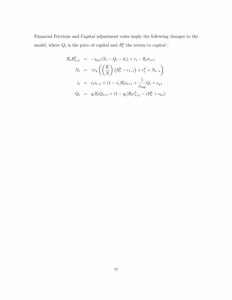
Financial Frictions and Capital adjustment costs imply the following changes to the

model, where Qt is the price of capital and Rkt the return to capital :

EtRkt`1 “ ´χprpNt ´Qt ´ ktq ` rt ´ Etπt`1

Nt “ γrk

ˆˆ

K

N

˙

`

Rkt ´ rt´1

˘

` rkt `Nt´1

˙

it “ i1it´1 ` p1´ i1qEtit`1 `1φadj

Qt ` εq,t

Qt “ q1EtQt`1 ` p1´ q1qEtrkt`1 ´ pRkt ` εb,tq

57

Table 1. Confidence Set for ΘIM and ΘCM -with survey data

Incomplete Model Complete ModelParameter q2.5% q97.5% q5% q95%

σc 12.460 13.320 28.6900 30.0000φp 5.1840 5.3430 21.5700 21.7000gy 0.9668 1.0000 0.2432 0.4827λh 0.7550 0.7673 0.0009 0.0009σl 8.5140 8.5760 8.892 9.104ξp 0.3654 0.3846 0.0000 0.0000ξw 0.0945 0.0958 0.8173 0.8628ιw 0.5631 0.575 0.9748 0.9999ιp 0.4952 0.498 0.0004 0.0004z1 0.5360 0.5429 0.0009 0.0009ρa 0.6447 0.6504 0.7521 0.9092ρb 0.6729 0.6789 0.0000 0.0000ρg 0.0000 0.0023 0.9999 0.9999ρqs 0.3394 0.3468 0.3242 0.4079ρms 0.4044 0.4137 0.7347 0.8015ρp 0.4802 0.4843 0.6329 0.7077ρw 0.2690 0.2719 0.0003 0.0003map 0.9958 1.000 0.0129 0.0561maw 0.5466 0.5487 0.0010 0.0011ν 0.6084 0.6104 0.0053 0.0205ρy‹ 0.6080 0.6080 0.1683 0.2251σa 9.8980 20.000 0.0245 0.0339σb 3.8910 7.3910 3.4480 3.4800σg 13.530 13.830 4.5820 4.6340σqs 9.2380 15.23 0.1831 0.2064σm 9.1220 10.240 1.0250 1.0670σp 0.9563 1.9220 4.2260 4.2660σw - - - -σf - - - -φadj - - 5.9210 5.9550χpr - - 0.9862 0.9999γ - - 0.9944 0.9950

KN - - 4.3330 4.3490

Note: σw and σf are set to 1. Parameters in italic font reached the boundary and

thus calibrated to the boundary value.

58

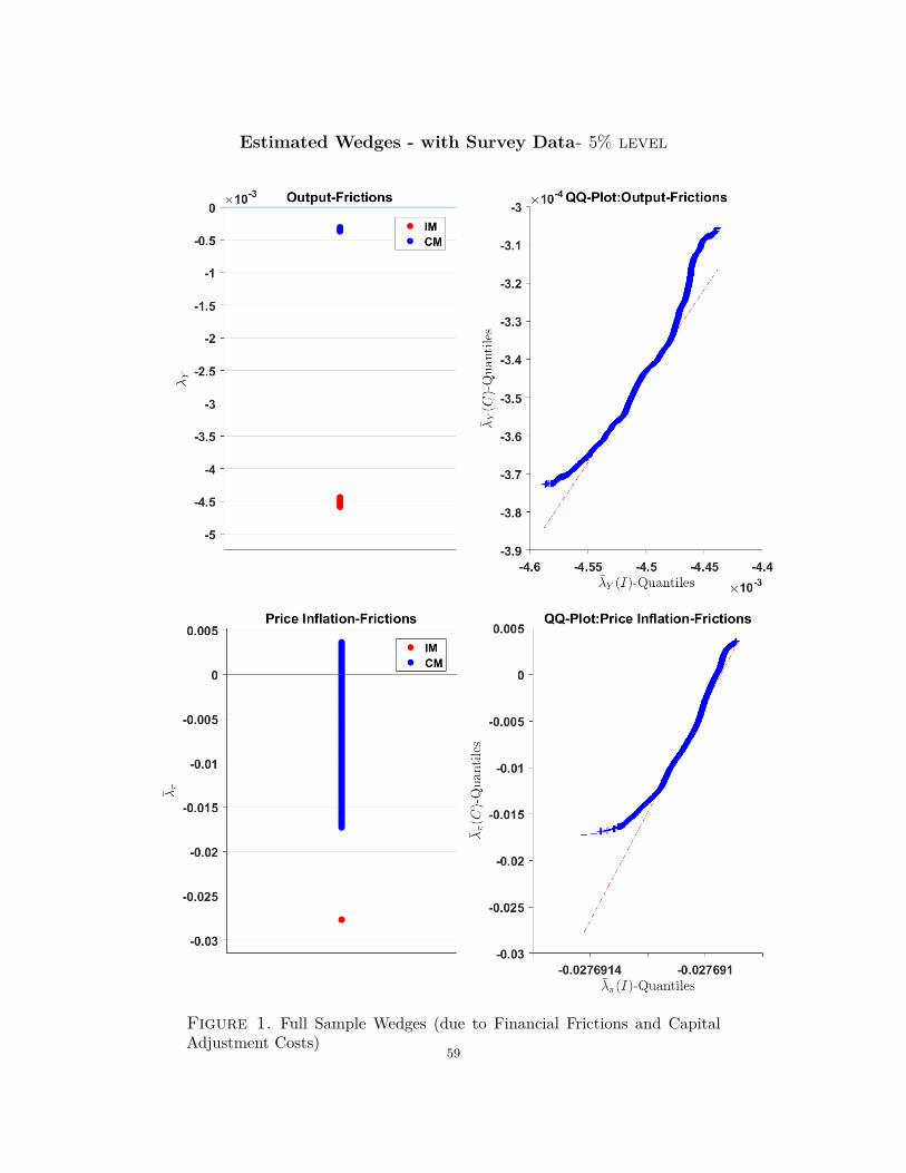
Estimated Wedges - with Survey Data- 5% level

Figure 1. Full Sample Wedges (due to Financial Frictions and CapitalAdjustment Costs)

59

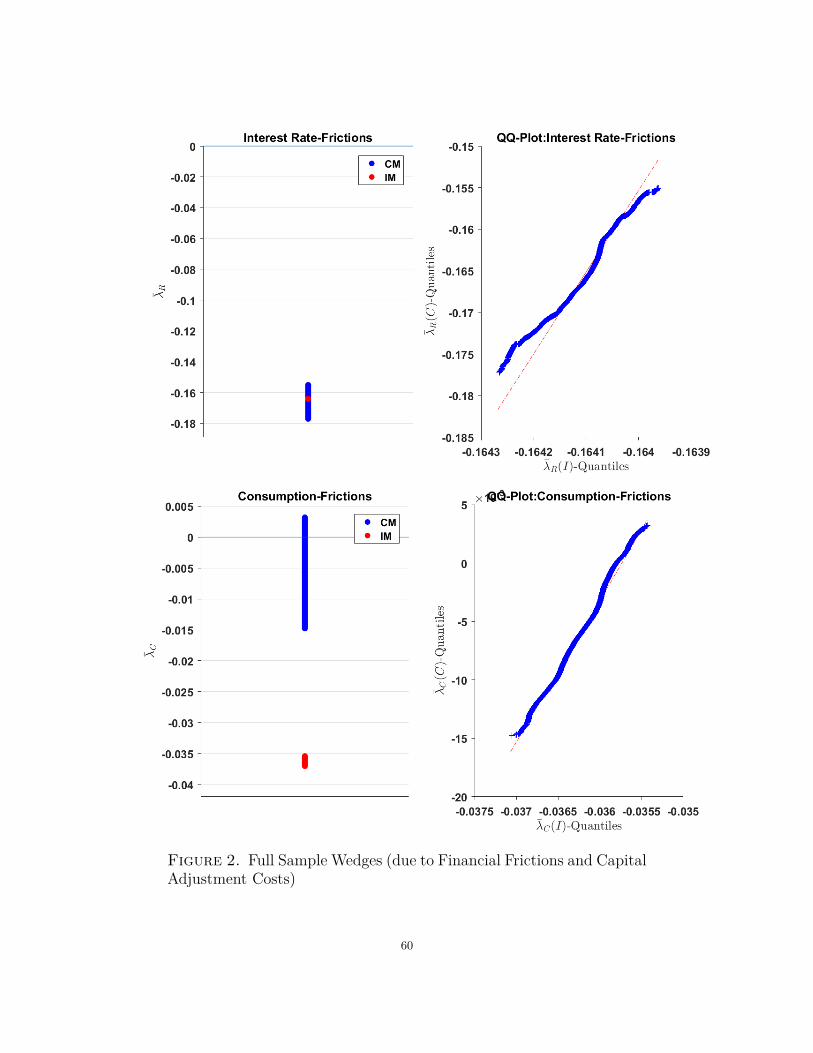
Figure 2. Full Sample Wedges (due to Financial Frictions and CapitalAdjustment Costs)

60

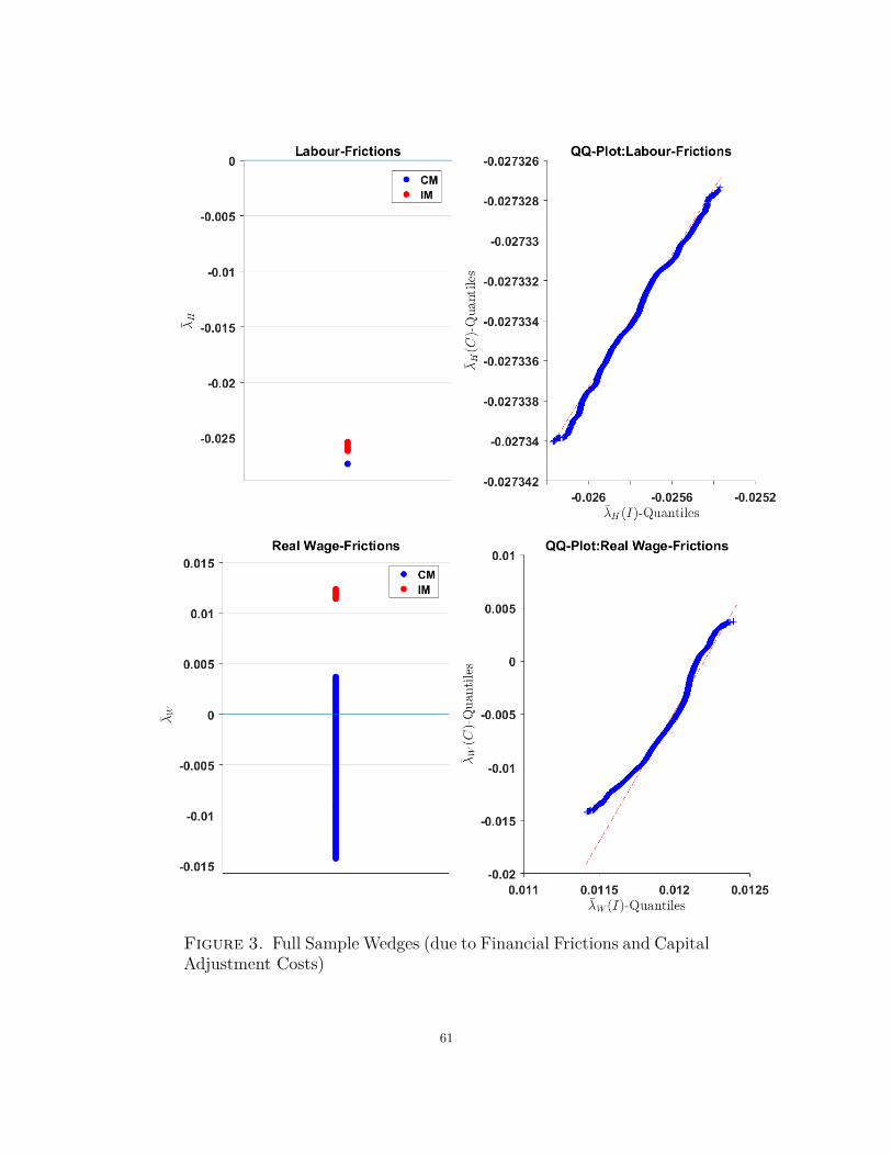
Figure 3. Full Sample Wedges (due to Financial Frictions and CapitalAdjustment Costs)

61

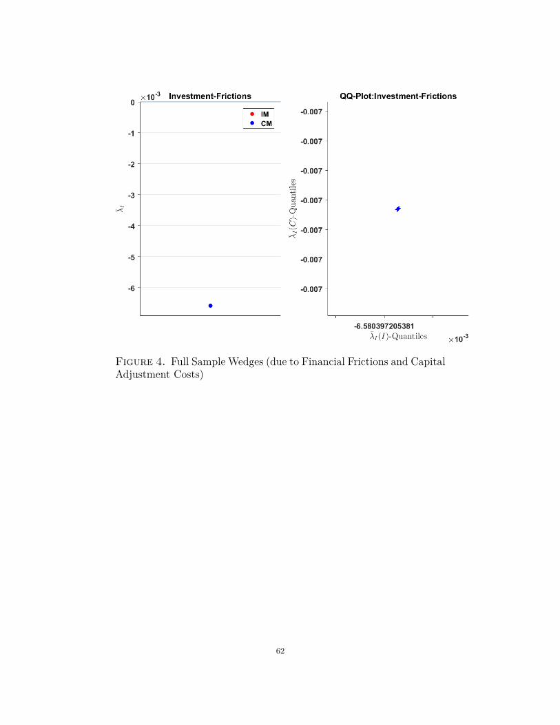
Figure 4. Full Sample Wedges (due to Financial Frictions and CapitalAdjustment Costs)

62