Set Theory and Algebra in Computer Science

A Gentle Introduction to Mathematical Modeling

Jose MeseguerUniversity of Illinois at Urbana-Champaign

Urbana, IL 61801, USA

c© Jose Meseguer, 2008–2013; all rights reserved.

August 28, 2013

2

Contents

I Basic Set Theory 5

1 Introduction to Part I 7

2 Set Theory as an Axiomatic Theory 11

3 The Empty Set, Extensionality, and Separation 153.1 The Empty Set . . . . . . . . . . . . . . . . . . . . . . . . . . . . . . . . . . . . . . . . 153.2 Extensionality . . . . . . . . . . . . . . . . . . . . . . . . . . . . . . . . . . . . . . . . . 153.3 The Failed Attempt of Comprehension . . . . . . . . . . . . . . . . . . . . . . . . . . . . 163.4 Separation . . . . . . . . . . . . . . . . . . . . . . . . . . . . . . . . . . . . . . . . . . . 17

4 Pairing, Unions, Powersets, and Infinity 194.1 Pairing . . . . . . . . . . . . . . . . . . . . . . . . . . . . . . . . . . . . . . . . . . . . . 194.2 Unions . . . . . . . . . . . . . . . . . . . . . . . . . . . . . . . . . . . . . . . . . . . . . 214.3 Powersets . . . . . . . . . . . . . . . . . . . . . . . . . . . . . . . . . . . . . . . . . . . 244.4 Infinity . . . . . . . . . . . . . . . . . . . . . . . . . . . . . . . . . . . . . . . . . . . . . 26

5 Relations, Functions, and Function Sets 295.1 Relations and Functions . . . . . . . . . . . . . . . . . . . . . . . . . . . . . . . . . . . . 295.2 Formula, Assignment, and Lambda Notations . . . . . . . . . . . . . . . . . . . . . . . . 305.3 Images . . . . . . . . . . . . . . . . . . . . . . . . . . . . . . . . . . . . . . . . . . . . . 325.4 Composing Relations and Functions . . . . . . . . . . . . . . . . . . . . . . . . . . . . . 335.5 Abstract Products and Disjoint Unions . . . . . . . . . . . . . . . . . . . . . . . . . . . . 375.6 Relating Function Sets . . . . . . . . . . . . . . . . . . . . . . . . . . . . . . . . . . . . 39

6 Simple and Primitive Recursion, and the Peano Axioms 436.1 Simple Recursion . . . . . . . . . . . . . . . . . . . . . . . . . . . . . . . . . . . . . . . 436.2 Primitive Recursion . . . . . . . . . . . . . . . . . . . . . . . . . . . . . . . . . . . . . . 456.3 The Peano Axioms . . . . . . . . . . . . . . . . . . . . . . . . . . . . . . . . . . . . . . 47

7 Binary Relations on a Set 497.1 Directed and Undirected Graphs . . . . . . . . . . . . . . . . . . . . . . . . . . . . . . . 497.2 Transition Systems and Automata . . . . . . . . . . . . . . . . . . . . . . . . . . . . . . 517.3 Relation Homomorphisms and Simulations . . . . . . . . . . . . . . . . . . . . . . . . . 527.4 Orders . . . . . . . . . . . . . . . . . . . . . . . . . . . . . . . . . . . . . . . . . . . . . 547.5 Sups and Infs, Complete Posets, Lattices, and Fixpoints . . . . . . . . . . . . . . . . . . . 577.6 Equivalence Relations and Quotients . . . . . . . . . . . . . . . . . . . . . . . . . . . . . 597.7 Constructing Z and Q . . . . . . . . . . . . . . . . . . . . . . . . . . . . . . . . . . . . . 63

8 Sets Come in Different Sizes 658.1 Cantor’s Theorem . . . . . . . . . . . . . . . . . . . . . . . . . . . . . . . . . . . . . . . 658.2 The Schroeder-Bernstein Theorem . . . . . . . . . . . . . . . . . . . . . . . . . . . . . . 66

3

9 Indexed Sets 679.1 Indexed Sets are Surjective Functions . . . . . . . . . . . . . . . . . . . . . . . . . . . . 679.2 Constructing Indexed Sets from other Indexed Sets . . . . . . . . . . . . . . . . . . . . . 719.3 Indexed Relations and Functions . . . . . . . . . . . . . . . . . . . . . . . . . . . . . . . 72

10 From Indexed Sets to Sets, and the Axiom of Choice 7510.1 Some Constructions Associating a Set to an Indexed Set . . . . . . . . . . . . . . . . . . 7510.2 The Axiom of Choice . . . . . . . . . . . . . . . . . . . . . . . . . . . . . . . . . . . . . 79

11 Well-Founded Relations, and Well-Founded Induction and Recursion 8311.1 Well-Founded Relations . . . . . . . . . . . . . . . . . . . . . . . . . . . . . . . . . . . 83

11.1.1 Constructing Well-Founded Relations . . . . . . . . . . . . . . . . . . . . . . . . 8411.2 Well-Founded Induction . . . . . . . . . . . . . . . . . . . . . . . . . . . . . . . . . . . 8511.3 Well-Founded Recursion . . . . . . . . . . . . . . . . . . . . . . . . . . . . . . . . . . . 86

11.3.1 Examples of Well-Founded Recursion . . . . . . . . . . . . . . . . . . . . . . . . 8611.3.2 Well-Founded Recursive Definitions: Step Functions . . . . . . . . . . . . . . . . 8611.3.3 The Well-Founded Recursion Theorem . . . . . . . . . . . . . . . . . . . . . . . 88

II Universal Algebra, Equational Logic and Term Rewriting 89

12 Algebras 9112.1 Unsorted Σ-Algebras . . . . . . . . . . . . . . . . . . . . . . . . . . . . . . . . . . . . . 9212.2 Many-Sorted Σ-Algebras . . . . . . . . . . . . . . . . . . . . . . . . . . . . . . . . . . . 9312.3 Order-Sorted Σ-Algebras . . . . . . . . . . . . . . . . . . . . . . . . . . . . . . . . . . . 9412.4 Terms and Term Algebras . . . . . . . . . . . . . . . . . . . . . . . . . . . . . . . . . . . 9612.5 A Set-Theoretic Construction of Term Algebras . . . . . . . . . . . . . . . . . . . . . . . 9712.6 More on Order-Sorted Signatures . . . . . . . . . . . . . . . . . . . . . . . . . . . . . . . 99

13 Term Rewriting and Equational Logic 10313.1 Terms, Equations, and Term Rewriting . . . . . . . . . . . . . . . . . . . . . . . . . . . . 103

13.1.1 Term Rewriting . . . . . . . . . . . . . . . . . . . . . . . . . . . . . . . . . . . . 10413.1.2 Equational Proofs . . . . . . . . . . . . . . . . . . . . . . . . . . . . . . . . . . . 105

13.2 Term Rewriting and Equational Reasoning Modulo Axioms . . . . . . . . . . . . . . . . . 10613.3 Sort-Decreasingness, Confluence, and Termination . . . . . . . . . . . . . . . . . . . . . 10813.4 Canonical Term Algebras . . . . . . . . . . . . . . . . . . . . . . . . . . . . . . . . . . . 11113.5 Sufficient Completeness . . . . . . . . . . . . . . . . . . . . . . . . . . . . . . . . . . . . 112

14 Conditional Rewriting and Conditional Equational Logic 11514.1 Conditional Term Rewriting and Conditional Equality . . . . . . . . . . . . . . . . . . . . 115

14.1.1 Conditional Term Rewriting and Conditional Equality as Inference . . . . . . . . . 11614.1.2 Proofs for Conditional Term Rewriting and Conditional Equality . . . . . . . . . . 117

14.2 Conditional Term Rewriting Modulo Axioms . . . . . . . . . . . . . . . . . . . . . . . . 12014.3 Executability Conditions for Conditional Rewrite Theories . . . . . . . . . . . . . . . . . 121

14.3.1 Confluence and the Church-Rosser Property in the Conditional Case . . . . . . . . 12114.3.2 Operational Termination . . . . . . . . . . . . . . . . . . . . . . . . . . . . . . . 122

4

Part I

Basic Set Theory

5

Chapter 1

Introduction to Part I

“... we cannot improve the language of any science without at the same time improving thescience itself; neither can we, on the other hand, improve a science, without improving thelanguage or nomenclature which belongs to it.”(Lavoisier, 1790, quoted in Goldenfeld and Woese [23])

I found the inadequacy of language to be an obstacle; no matter how unwieldly the expressionsI was ready to accept, I was less and less able, as the relations became more and more complex,to attain the precision that my purpose required. This deficiency led me to the idea of thepresent ideography. . . . I believe that I can best make the relation of my ideography to ordinarylanguage clear if I compare it to that which the microscope has to the eye. Because of the rangeof its possible uses and the versatility with which it can adapt to the most diverse circumstances,the eye is far superior to the microscope. Considered as an optical instrument, to be sure, itexhibits many imperfections, which ordinarily remain unnoticed only on account of its intimateconnection with our mental life. But, as soon as scientific goals demand great sharpness ofresolution, the eye proves to be insufficient. The microscope, on the other hand, is prefectlysuited to precisely such goals, but that is just why it is useless for all others.(Frege, 1897, Begriffsschrift, in [47], 5–6)

Language and thought are related in a deep way. Without any language it may become impossible toconceive and express any thoughts. In ordinary life we use the different natural languages spoken on theplanet. But natural language, although extremely flexible, can be highly ambiguous, and it is not at all wellsuited for science. Imagine, for example, the task of professionally developing quantum mechanics (itselfrelying on very abstract concepts, such as those in the mathematical language of operators in a Hilbertspace) in ordinary English. Such a task would be virtually impossible; indeed, ridiculous: as preposterousas trying to build the Eiffel tower in the Sahara desert with blocks of vanilla ice cream. Even the task ofpopularization, that is, of explaining informally in ordinary English what quantum mechanics is, is highlynontrivial, and must of necessity remain suggestive, metaphorical, and fraught with the possibility of grossmisunderstandings.

The point is that without a precise scientific language it becomes virtually impossible, or at least enor-mously burdensome and awkward, to think scientifically. This is particularly true in mathematics. Oneof the crowning scientific achievements of the 20th century was the development of set theory as a pre-cise language for all of mathematics, thanks to the efforts of Cantor, Dedekind, Frege, Peano, Russell andWhitehead, Zermelo, Fraenkel, Skolem, Hilbert, von Neumann, Godel, Bernays, Cohen, and others. Thisachievement has been so important and definitive that it led David Hilbert to say, already in 1925, that “noone will drive us from the paradise which Cantor created for us” (see [47], 367–392, pg. 376). It was of

7

course possible to think mathematically before set theory, but in a considerably more awkward and quiterestricted way, because the levels of generality, rigor and abstraction made possible by set theory are muchgreater than at any other previous time. In fact, many key mathematical concepts we now take for granted,such a those of an abstract group or a topological space, could only be formulated after set theory, preciselybecause the language needed to conceive and articulate those concepts was not available before.

Set theory is not really the only rigorous mathematical language. The languages of set theory and ofmathematical logic were developed together, so that, as a mathematical discipline, set theory is a branch ofmathematical logic. Technically, as we shall see shortly, we can view the language of set theory as a specialsublanguage of first-order logic. Furthermore, other theories such as category theory and intuitionistic typetheory have been proposed as alternatives to set theory to express all of mathematics.

There are various precise logical formalisms other than set theory which are particularly well-suited toexpress specific concepts in a given domain of thought. For example, temporal logic is quite well-suited toexpress properties satisfied by the dynamic behavior of a concurrent system; and both equational logic andthe lambda calculus are very well suited to deal with functions and functional computation. However, settheory plays a privileged role as a mathematical language in which all the mathematical structures we needin order to give a precise meaning to the models described by various other logical languages, and to thesatisfaction of formulas in such languages, can be defined.

All this has a direct bearing on the task of formal software specification and verification. Such a taskwould be meaningless, indeed utter nonsense and voodoo superstition, without the use of mathematicalmodels and mathematical logic. And it is virtually impossible, or extremely awkward, to even say whatneeds to be said about such mathematical models and logical properties without a precise mathematicallanguage. More importantly, it becomes virtually impossible to think properly without the conceptual toolsprovided by such a language. Either set theory or some comparable language become unavoidable: it ispart of what any well educated computer scientist should be conversant with, like the air one breathes.

These notes include a review of basic set theory concepts that any well educated computer scientistshould be familiar with. Although they go beyond reviewing basic knowledge in various ways, nothingexcept basic acquaintance with the use of logical connectives and of universal and existential quantificationin logic is assumed: the presentation is entirely self-contained, and many exercises are proposed to helpthe reader sharpen his/her understanding of the basic concepts. The exercises are an essential part of thesenotes, both because they are used in proofs of quite a few theorems, and because by solving problems in amathematical theory one avoids having a superficial illusion of understanding, and gains real understanding.For those already well-versed in elementary set theory, these notes can be read rather quickly. However,some topics such as well-founded relations, well-founded induction, well-founded recursive functions, andI-indexed sets may be less familiar. Also, already familiar notions are here presented in a precise, axiomaticway. This may help even some readers already thoroughly familiar with “naive” set theory gain a moredetailed understanding of it as a logically axiomatized theory. Becoming used to reason correctly withinan axiomatic theory —Euclidean geometry is the classical example, and axiomatic set theory follows thesame conceptual pattern— is the best way I know of learning to think in a precise, mathematical way.Furthermore, a number of useful connections between set theory and computer science are made explicit inthese notes; connections that are usually not developed in standard presentations of set theory.

I should add some final remarks on the style of these notes. There are three particular stylistic featuresthat I would like to explain. First, these notes take the form of an extended conversation with the reader, inwhich I propose and discuss various problems, why they matter, and throw out ideas on how to solve suchproblems. This is because I believe that science itself is an ongoing critical dialogue, and asking questionsin a probing way is the best way to understand anything. Second, I do not assume the proverbial mathemat-ical maturity on the part of the reader, since such maturity is precisely the quod erat demonstrandum, andbringing it about is one of the main goals of these notes: I am convinced that in the 21st century mathemati-cal maturity is virtually impossible without mastering the language of set theory. On the contrary, I assumethe potential mathematical immaturity of some readers. This means that, particularly in the early chapters,there is a generous amount of what might be called mathematical spoon feeding, hand holding, and evena few nursery tales. This does not go on forever, since at each stage I assume as known all that has beenalready presented, that is, the mastery of the language already covered, so that in more advanced chapters,although the conversational style, examples, and motivation remain, the discourse gradually becomes moremature.

8

The third stylistic feature I want to discuss is that the mindset of category theory, pervasive in modernmathematics, is present everywhere in these notes, but in Parts I and II this happens in a subliminal way.Categories and functors will be defined in Part III; but they are present from the beginning like a hidden mu-sic. And functorial constructions make early cameo appearances in Part I (very much like Alfred Hitchcockin his own movies) in several exercises.

9

10

Chapter 2

Set Theory as an Axiomatic Theory

In mathematics all entities are studied following a very successful method, which goes back at least toEuclid, called the axiomatic method. The entities in question, for example, points, lines, and planes (ornumbers, or real-valued functions, or vector spaces), are characterized by means of axioms that are postu-lated about them. Then one uses logical deduction to infer from those axioms the properties that the entitiesin question satisfy. Such properties, inferred from the basic axioms, are called theorems. The axioms,together with the theorems we can prove as their logical consequences, form a mathematical, axiomatictheory. It is in this sense that we speak of group theory, the theory of vector spaces, probability theory,recursion theory, the theory of differentiable real-valued functions, or set theory.

The way in which set theory is used as a language for mathematics is by expressing or translating othertheories in terms of the theory of sets. In this way, everything can be reduced to sets and relations betweensets. For example, a line can be precisely understood as a set of points satisfying certain properties. Andpoints themselves (for example, in 3-dimensional space) can be precisely understood as triples (anotherkind of set) of real numbers (the point’s coordinates). And real numbers themselves can also be preciselyunderstood as sets of a different kind (for example as “Dedekind cuts”). In the end, all sets can be built outof the empty set, which has no elements. So all of mathematics can in this way be constructed, as it were,ex nihilo.

But sets themselves are also mathematical entities, which in this particular encoding of everything assets we happen to take as the most basic entities.1 This means that we can study sets also axiomatically, justas we study any other mathematical entity: as things that satisfy certain axioms. In this way we can provetheorems about sets: such theorems are the theorems of set theory. We shall encounter some elementary settheory theorems in what follows. Since set theory is a highly developed field of study within mathematics,there are of course many other theorems which are not discussed here: our main interest is not in set theoryitself, but in its use as a mathematical modeling language, particularly in computer science.

Mathematical logic, specifically the language of first-order logic, allows us to define axiomatic theories,and then logically deduce theorems about such theories. Each first-order logic theory has an associatedformal language, obtained by specifying its constants (for example, 0) and function symbols (for example,+ and · for the theory of numbers), and its predicate symbols (for example, a strict ordering predicate >).Then, out of the constants, function symbols, and variables we build terms (for example, (x + 0) · y, and(x+y) ·z are terms). By plugging terms as arguments into predicate symbols, we build the atomic predicates(for example, (x + y) > 0 is an atomic predicate). And out of the atomic predicates we build formulas bymeans of the logical connectives of conjunction (∧), disjunction (∨), negation (¬), implication (⇒), andequivalence (⇔); and of universal (∀) and existential (∃) quantification, to which we also add the “thereexists a unique” (∃!) existential quantification variant. For example, the formula

(∀x)(x > 0⇒ (x + x) > x)

says that for each element x strictly greater than 0, x + x is strictly greater than x. This is in fact a theorem

1What things to take as the most basic entities is itself a matter of choice. All of mathematics can be alternatively developed in thelanguage of category theory (another axiomatic theory); so that sets themselves then appear as another kind of entity reducible to thelanguage of categories, namely, as objects in the category of sets (see, e.g., [29, 30] and [32] VI.10).

11

for the natural numbers. Similarly, the formula

(∀x)(∀y)(y > 0 ⇒ ((∃!q)(∃!r)((x = (y · q) + r) ∧ (y > r))))

says that for all x and y, if y > 0 then there exist unique q and r such that x = (y · q) + r and y > r. Thisis of course also a theorem for the natural numbers, where we determine the unique numbers called thequotient q and the remainder r of dividing x by a nonzero number y by means of the division algorithm. Infirst-order logic it is customary to always throw in the equality predicate (=) as a built-in binary predicatein the language of formulas, in addition to the domain-specific predicates, such as >, of the given theory.This is indicated by speaking about first-order logic with equality.

In the formal language of set theory there are no function symbols and no constants, and only onedomain-specific binary predicate symbol, the ∈ symbol, read belongs to, or is a member of, or is an elementof, which holds true of an element x and a set X, written x ∈ X, if and only if x is indeed an element ofthe set X. This captures the intuitive notion of belonging to a “set” or “collection” of elements in ordinarylanguage. So, if Joe Smith is a member of a tennis club, then Joe Smith belongs to the set of members of thatclub. Similarly, 2, 3, and 5 are members of the set Prime of prime numbers, so we can write 2, 3, 5 ∈ Primeas an abbreviation for the logical conjunction (2 ∈ Prime) ∧ (3 ∈ Prime) ∧ (5 ∈ Prime). The language offirst-order formulas of set theory has then an easy description as the set of expressions that can be formedout of a countable set of variables x, y, z, x′, y′, z′, . . . and of smaller formulas ϕ, ϕ′, etc., by means of thefollowing BNF-like grammar:

x ∈ y | x = y | (ϕ ∧ ϕ′) | (ϕ ∨ ϕ′) | (ϕ⇒ ϕ′) | (ϕ⇔ ϕ′) | ¬(ϕ) | (∀x)ϕ | (∃x)ϕ | (∃!x)ϕ

where we allow some abbreviations: ¬(x = y) can be abbreviated by x , y; ¬(x ∈ y) can be abbreviatedby x < y; ¬((∃x)ϕ) can be abbreviated by (@x)ϕ (and is logically equivalent to (∀x)¬(ϕ)); (∀x1) . . . (∀xn)ϕ,respectively (∃x1) . . . (∃xn)ϕ, can be abbreviated by (∀x1, . . . , xn)ϕ, respectively (∃x1, . . . , xn)ϕ; and x1 ∈

y ∧ . . . ∧ xn ∈ y can be abbreviated by x1, . . . , xn ∈ y.As in any other first-order language, given a formula ϕ we can distinguish between variables that are

quantified in ϕ, called bound variables, unquantified variables, called free variables. For example, in theformula (∃x) x ∈ y, x is bound by the ∃ quantifier, and y is free. More precisely, for x and y any twovariables (including the case when x and y are the same variable):

• x and y are the only free variables in x ∈ y and in x = y

• x is a free variable of ¬(ϕ) iff2 x is a free variable of ϕ

• x is a free variable of ϕ ∧ ϕ′ (resp. ϕ ∨ ϕ′, ϕ ⇒ ϕ′, ϕ ⇔ ϕ′) iff x is a free variable of ϕ or x is a freevariable of ϕ′

• x is neither a free variable of (∀x)ϕ, nor of (∃x)ϕ, nor of (∃!x)ϕ; we say that x is bound in thesequantified formulas.

For example, in the formula (∀x)(x = y ⇒ x < y) the variable x is bound, and the variable y is free, so y isthe only free variable.

Set theory is then specified by its axioms, that is, by some formulas in the above language that arepostulated as true for all sets. These are the axioms (∅), (Ext), (Sep), (Pair), (Union), (Pow), (Inf ), (AC),(Rep), and (Found). All of them, except for (Rep) and (Found), will be stated and explained in the followingchapters. The above set of axioms is usually denoted ZFC (Zermelo Fraenkel set theory with Choice).ZFC minus the Axiom of Choice (AC) is denoted ZF. As the axioms are introduced, we will derive sometheorems that follow logically as consequences from the axioms. Other such theorems will be developed inexercises left for the reader.

The above set theory language is what is called the language of pure set theory, in which all elements ofa set are themselves simpler sets. Therefore, in pure set theory quantifying over elements and quantifyingover sets is exactly the same thing,3 which is convenient. There are variants of set theory where primitiveelements which are not sets (called atoms or urelements) are allowed (this is further discussed in §??).

2Here and everywhere else in these notes, “iff” is always an abbreviation for “if and only if.”3Of course, this would not be the same thing if we were to quantify only over the elements of a fixed set, say A, as in a formula such

as (∀x ∈ A) x , ∅. But note that, strictly speaking, such a formula does not belong to our language: it is just a notational abbreviationfor the formula (∀x) ((x ∈ A) ⇒ (x , ∅)), in which x is now universally quantified over all sets.

12

Let us now consider the process of logical deduction. Any first-order logic theory is specified by thelanguage L of its formulas (in our case, the above language of set theory formulas), and by a set Γ ofaxioms, that is, by a set Γ of formulas in the language L, which are adopted as the axioms of the theory(in our case, Γ is the set ZFC of Zermelo-Fraenkel axioms). Given any such theory with axioms Γ, first-order logic provides a finite set of logical inference rules that allow us to derive all true theorems (and onlytrue theorems) of the theory Γ. Using these inference rules we can construct proofs, which show how wecan reason logically from the axioms Γ to obtain a given theorem ϕ by finite application of the rules. If aformula ϕ can be proved from the axioms Γ by such a finite number of logical steps, we use the notationΓ ` ϕ, read, Γ proves (or entails) ϕ, and call ϕ a theorem of Γ. For example, the theorems of set theory areprecisely the formulas ϕ in the above-defined language of set theory such that ZFC ` ϕ. Similarly, if GP isthe set of axioms of group theory, then the theorems of group theory are the formulas ϕ in GP’s languagesuch that GP ` ϕ.

A very nice feature of the logical inference rules is that they are entirely mechanical, that is, theyprecisely specify concrete, syntax-based steps that can be carried out mechanically by a machine such as acomputer program. Such computer programs are called theorem provers (or sometimes proof assistants);they can prove theorems from Γ either totally automatically, or with user guidance about what logicalinference rules (or combinations of such rules) to apply to a given formula. For example, one such inferencerule (a rule for conjunction introduction) may be used when we have already proved theorems Γ ` ϕ, andΓ ` ψ, to obtain the formula ϕ ∧ ψ as a new theorem. Such a logical inference rule is typically written

Γ ` ϕ Γ ` ψ

Γ ` ϕ ∧ ψ

where Γ, ϕ, ψ, are completely generic; that is, the above rule applies to the axioms Γ of any theory, andto any two proofs Γ ` ϕ and Γ ` ψ of any formulas ϕ and ψ as theorems from Γ; it can then be used toderive the formula ϕ ∧ ψ as a new theorem of Γ. Therefore, the collection of proofs above the vertical barof such inference rules tells us what kinds of theorems we have already derived, and then what is writtenbelow an horizontal bar yields a new theorem, which we can derive as a logical consequence of theoremsalready derived. There are several logical inference systems, that is, several collections of logical inferencerules for first-order logic, all of equivalent proving power (that is, all prove the same theorems, and exactlythe true theorems); however, some inference systems are easier to use by humans than others. A very gooddiscussion of such inference systems, and of first-order logic, can be found in [3].

In actual mathematical practice, proofs of theorems are not fully formalized; that is, an explicit con-struction of a proof as the result of a mechanical inference process from the axioms Γ is typically not given;instead, and informal but rigorous high-level description of the proof is given. This is because a detailedformal proof may involve a large amount of trivial details that are perfectly fine for a computer to take careof, but would make a standard hundred-page mathematical book run for many thousands of pages. How-ever, the informal mathematical proofs are only correct provided that in principle, if the proponent of theproof is challenged, he or she could carry out a detailed formal, and machine verifiable proof leading to thetheorem from the axioms by means of the rules of logical deduction. In Part I we will follow the standardmathematical practice of giving rigorous but informal proofs. However, in Part II proofs in equational logic(a sublogic of first-order logic) will be fully formalized, and the soundness and completeness of equationallogic (the fact that it can prove only true theorems, and all true theorems) will be proved in detail.

13

14

Chapter 3

The Empty Set, Extensionality, andSeparation

3.1 The Empty SetThe simplest, most basic axiom, the empty set axiom, can be stated in plain English by saying:

There is a set that has no elements.

This can be precisely captured by the following set theory formula, which we will refer to as the (∅) axiom:

(∅) (∃x)(∀y) y < x.

It is very convenient to introduce an auxiliary notation for such a set, which is usually denoted by ∅. Sincesets are typically written enclosing their elements inside curly brackets, thus 1, 2, 3 to denote the set whoseelements are 1, 2, and 3, a more suggestive notation for the empty set would have been . That is, we canthink of the curly brackets as a “box” in which we store the elements, so that when we open the box thereis nothing in it! However, since the ∅ notation is so universally accepted, we will stick with it anyway.

3.2 ExtensionalityAt this point, the following doubt could arise: could there be several empty sets? If that were the case, our∅ notation would be ambiguous. This doubt can be put to rest by a second axiom of set theory, the axiomof extensionality, which allows us to determine when two sets are equal. In plain English the extensionalityaxiom can be stated as follows:

Two sets are equal if and only if they have the same elements.

Again, this can be precisely captured by the following formula in our language, which we will refer to asthe (Ext) axiom:

(Ext) (∀x, y)((∀z)(z ∈ x⇔ z ∈ y)⇒ x = y)

where it is enough to have the implication⇒ in the formula, instead of the equivalence⇔, because if twosets are indeed equal, then logical reasoning alone ensures that they must have the same elements, that is,we get the other implication⇐ for free, so that it needs not be explicitly stated in the axiom. Note that, asalready mentioned, extensionality makes sure that our ∅ notation for the empty set is unambiguous, sincethere is only one such set. Indeed, suppose that we were to have two empty sets, say ∅1 and ∅2. Then sinceneither of them have any elements, we of course have the equivalence (∀z)(z ∈ ∅1 ⇔ z ∈ ∅2). But then(Ext) forces the equality ∅1 = ∅2.

The word “extensionality” comes from a conceptual distinction between a formula as a linguistic de-scription and its “extension” as the collection of elements for which the formula is true. For example, in the

15

theory of the natural numbers, x > 0 and x + x > x are different formulas, but they have the same exten-sion, namely, the nonzero natural numbers. Extension in this sense is distinguished from “intension,” as theconceptual, linguistic description. For example, x > 0 and x + x > x are in principle different conceptualdescriptions, and therefore have different “intensions.” They just happen to have the same extension forthe natural numbers. But they may very well have different extensions in other models. For example, ifwe interpret + and > on the set 0, 1 with + interpreted as exclusive or, 1 > 0 true, and x > y false in theother three cases, then the extension of x > 0 is the singleton set 1, and the extension of x + x > x is theempty set. As we shall see shortly, in set theory we are able to define sets by different syntactic expressionsinvolving logical formulas. But the extension of a set expression is the collection of its elements. Theaxiom of extensionality axiomatizes the obvious, intuitive truism that two set expressions having the sameextension denote the same set.

The axiom of extensionality is intimately connected with the notion of a subset. Given two sets, A andB, we say that A is a subset of B, or that A is contained in B, or that B contains A, denoted A ⊆ B, if andonly if every element of A is an element of B. We can precisely define the subset concept in our formallanguage by means of the defining equivalence:

x ⊆ y ⇔ (∀z)(z ∈ x⇒ z ∈ y).

Using this abbreviated notation we can then express the equivalence (∀z)(z ∈ x⇔ z ∈ y) as the conjunction(x ⊆ y ∧ y ⊆ x). This allows us to rephrase the (Ext) axiom as the implication:

(∀x, y)((x ⊆ y ∧ y ⊆ x)⇒ x = y)

which gives us a very useful method for proving that two sets are equal: we just have to prove that each iscontained in the other.

We say that a subset inclusion A ⊆ B is strict if, in addition, A , B. We then use the notation A ⊂ B.That is, we can define x ⊂ y by the defining equivalence

x ⊂ y ⇔ (x , y ∧ (∀z)(z ∈ x⇒ z ∈ y)).

Exercise 1 Prove that for any set A, A ⊆ A; and that for any three sets A, B, and C, the following implications hold:

(A ⊆ B ∧ B ⊆ C) ⇒ A ⊆ C (A ⊂ B ∧ B ⊂ C) ⇒ A ⊂ C.

3.3 The Failed Attempt of ComprehensionOf course, with these two axioms alone we literally have almost nothing! More precisely, they only guar-antee the existence of the empty set ∅, which itself has nothing in it.1 The whole point of set theory as alanguage for mathematics is to have a very expressive language, in which any self-consistent mathematicalentity can be defined. Clearly, we need to have other, more powerful axioms for defining sets.

One appealing idea is that if we can think of some logical property, then we should be able to definethe set of all elements that satisfy that property. This idea was first axiomatized by Gottlob Frege at theend of the 19th century as the following axiom of comprehension, which in our contemporary notation canbe described as follows: given any set theory formula ϕ whose only free variable is x, there is a set whoseelements are those sets that satisfy ϕ. We would then denote such a set as follows: x | ϕ. In our set theorylanguage this can be precisely captured, not by a single formula, but by a parametric family of formulas,

1 It is like having just one box, which when we open it happens to be empty, in a world where two different boxes always containdifferent things (extensionality). Of course, in the physical world of physical boxes and physical objects, extensionality is always truefor nonempty boxes, since two physically different nonempty boxes, must necessarily contain different physical objects. For example,two different boxes may each just contain a dollar bill, but these must be different dollar bills. The analogy of a set as box, and of theelements of a set as the objects contained inside such a box (where those objects might sometimes be other (unopened) boxes) can behelpful but, although approximately correct, it is not literally true and could sometimes be misleading. In some senses, the physicalmetaphor is too loose; for example, in set theory there is only one empty set, but in the physical world we can have many empty boxes.In other senses the metaphor is too restrictive; for example, physical extensionality for nonempty boxes means that no object can beinside two different boxes, whereas in set theory the empty set (and other sets) can belong to (“be inside of”) several different setswithout any problem.

16

called an axiom scheme. Specifically, for each formula ϕ in our language whose only free variable is x, wewould add the axiom

(∃!y)(∀x)(x ∈ y⇔ ϕ)

and would then use the notation x | ϕ as an abbreviation for the unique y defined by the formula ϕ. Forexample, we could define in this way the set of all sets, let us call it the universe and denote it U , as the setdefined by the formula x = x, that is, U = x | x = x. Since obviously U = U , we have U ∈ U . Let uscall a set A circular iff A ∈ A. In particular, the universe U is a circular set.

Unfortunately for Frege, his comprehension axiom was inconsistent. This was politely pointed out in1902 by Bertrand Russell in a letter to Frege (see [47], 124–125). The key observation of Russell’s wasthat we could use Frege’s comprehension axiom to define the set of noncircular sets as the unique set NCdefined by the formula x < x. That is, NC = x | x < x. Russell’s proof of the inconsistency of Frege’ssystem, his “paradox,” is contained in the killer question: is NC itself noncircular? That is, do we haveNC ∈ NC? Well, this is just a matter of testing whether NC itself satisfies the formula defining NC, whichby the comprehension axiom gives us the equivalence:

NC ∈ NC ⇔ NC < NC

a vicious contradiction dashing to the ground the entire system built by Frege. Frege, who had investedmuch effort in his own theory and can be considered, together with the Italian Giuseppe Peano and theAmerican Charles Sanders Peirce, as one of the founders of what later came to be known as first-order logic,was devastated by this refutation of his entire logical system and never quite managed to recover from it.Russell’s paradox (and similar paradoxes emerging at that time, such as the Burali-Forti paradox (see [47],104–112), showed that we shouldn’t use set theory formulas to define other sets in the freewheeling waythat the comprehension axiom allows us to do: the concept of a set whose elements are those sets that arenot members of themselves is inconsistent; because if such a set belongs to itself, then it does not belong toitself, and vice versa. The problem with the comprehension axiom is its unrestricted quantification over allsets x satisfying the property ϕ(x).

Set theory originated with Cantor (see [9] for an excellent and very readable reference), and Dedekind.After the set theory paradoxes made the “foundations problem” a burning, life or death issue, all subsequentaxiomatic work in set theory has walked a tight rope, trying to find safe restrictions of the comprehensionaxiom that do not lead to contradictions, yet allow us as much flexibility as possible in defining any self-consistent mathematical notion. Russell proposed in 1908 his own solution, which bans sets that can bemembers of themselves by introducing a theory of types (see [47], 150–182). A simpler solution was giventhe same year by Zermelo (see [47], 199–215), and was subsequently formalized and refined by Skolem(see [47], 290–301), and Fraenkel (see [47], 284–289), leading to the so-called Zermelo-Fraenkel set theory(ZFC). ZFC should more properly be called Zermelo-Skolem-Fraenkel set theory and includes the already-given axioms (∅) and (Ext). In ZFC the comprehension axiom is restricted in various ways, all of themconsidered safe, since no contradiction of ZFC has ever been found, and various relative consistency resultshave been proved, showing for various subsets of axioms Γ ⊂ ZFC that if Γ is consistent (i.e., has nocontradictory consequences) then ZFC is also consistent.

3.4 SeparationThe first, most obvious restriction on the comprehension axiom is the so-called axiom of separation. Therestriction imposed by the separation axiom consists in requiring the quantification to range, not over allsets, but over the elements of some existing set. If A is a set and ϕ is a set theory formula having x as its onlyfree variable, then we can use ϕ to define the subset B of A whose elements are all the elements of A thatsatisfy the formula ϕ. We then describe such a subset with the notation x ∈ A | ϕ. For example, we candefine the set x ∈ ∅ | x < x, and this is a well-defined set (actually equal to ∅) involving no contradictionin spite of the dangerous-looking formula x < x.

Our previous discussion of extensionality using the predicates x > 0 and x + x > x can serve to illustratean interesting point about the definition of sets using the separation axiom. Assuming, as will be shownlater, that the set of natural numbers is definable as a setN in set theory, that any natural number is itself a set,and that natural number addition + and strict ordering on numbers > can be axiomatized in set theory, we

17

can then define the sets x ∈ N | x > 0 and x ∈ N | x + x > x. Note that, although as syntactic descriptionsthese expressions are different, as sets, since they have the same elements, the (Ext) axiom forces the setequality x ∈ N | x > 0 = x ∈ N | x + x > x. That is, we use a syntactic description involving the syntaxof a formula to denote an actual set, determined exclusively by its elements. In particular, formulas ϕ andϕ′ that are logically equivalent (for example, (φ ⇒ φ′) and (¬(φ) ∨ φ′) are logically equivalent formulas)always define by separation the same subset of the given set A, that is, if ϕ and ϕ′ are logically equivalentwe always have the equality of sets x ∈ A | ϕ = x ∈ A | ϕ′.

We can describe informally the separation axiom in English by saying:

Given any set A and any set theory formula ϕ(x) having x as its only free variable, we candefine a subset of A consisting of all elements x of A such that ϕ(x) is true.

The precise formalization of the separation axiom is as an axiom scheme parameterized by all set theoryformulas ϕ whose only free variable is x. For any such ϕ the separation axiom scheme adds the formula

(Sep) (∀y)(∃!z)(∀x)(x ∈ z⇔ (x ∈ y ∧ ϕ)).

The unique set z asserted to exist for each y by the above formula is then abbreviated with the notationx ∈ y | ϕ. But this notation does not yet describe a concrete set, since it has the variable y as parameter.That is, we first should choose a concrete set, say A, as the interpretation of the variable y, so that theexpression x ∈ A | ϕ then defines a corresponding concrete set, which is a subset of A. For this reason, theseparation axiom is sometimes called the subset axiom.

Jumping ahead a little, and assuming that we have already axiomatized the natural numbers in set theory(so that all number-theoretic notions and operations have been reduced to our set theory notation), we canillustrate the use of the (Sep) axiom by choosing as our ϕ the formula (∃y)(x = 3 · y). Then, denoting by Nthe set of natural numbers, the set x ∈ N | (∃y) (y ∈ N) ∧ (x = 3 · y) is the set of all multiples of 3.

Exercise 2 Assuming that the set N of natural numbers has been fully axiomatized in set theory, and in particular thatall the natural numbers 0, 1, 2, 3, etc., and the multiplication operation2 · on natural numbers have been axiomatizedin this way, write a formula that, using the axiom of separation, can be used to define the set of prime numbers as asubset of N.

Russell’s Paradox was based on the argument that the notion of a set NC of all noncircular sets isinconsistent. Does this also imply that the notion of a set U that is a universe, that is, a set of all sets is alsoinconsistent? Indeed it does.

Theorem 1 There is no set U of all sets. That is, the formula

(@U )(∀x) x ∈ U

is a theorem of set theory.

Proof. We reason by contradiction. Suppose such a set U exists. Then we can use (Sep) to define the set ofnoncircular sets as NC = x ∈ U | x < x, which immediately gives us a contradiction because of Russell’sParadox.

2Here and in what follows, I will indicate where the arguments of an operation like · or + appear by underbars, writing, e.g., · or+ . The same convention will be followed not just for basic operations but for more general functions; for example, multiplication

by 2 may be denoted 2 · .

18

Chapter 4

Pairing, Unions, Powersets, and Infinity

Although the separation axiom allows us to define many sets as subsets of other sets, since we still onlyhave the empty set, and this has no other subsets than itself, we clearly need other axioms to get the wholeset theory enterprise off the ground. The axioms of pairing, union, powerset, and infinity allow us to buildmany sets out of other sets, and, ultimately, ex nihilo, out of the empty set.

4.1 PairingOne very reasonable idea is to consider sets whose only element is another set. Such sets are called singletonsets. That is, if we have a set A, we can “put it inside a box” with curly brackets, say, A, so that when weopen the box there is only one thing in it, namely, A. The set A itself may be big, or small, or may even bethe empty set; but this does not matter: each set can be visualized as a “closed box,” so that when we openthe outer box A we get only one element, namely, the inner box A. As it turns out, with a single axiom,the axiom of pairing explained below, we can get two concepts for the price of one: singleton sets and(unordered) pairs of sets. That is, we can also get sets whose only elements are other sets A and B. Suchsets are called (unordered) pairs, and are denoted A, B. The idea is the same as before: we now enclose Aand B (each of which can be pictured as a closed box) inside the outer box A, B, which contains exactlytwo elements: A and B, provided A , B. What about A, A? That is, what happens if we try to encloseA twice inside the outer box? Well, this set expression still contains only one element, namely A, so that,by extensionality, A, A = A. That is, we get the notion of a singleton set as a special case of the notionof a pair. But this is all still just an intuitive, pretheoretic motivation: we need to define unordered pairsprecisely in our language.

In plain English, the axiom of pairing says:

Given sets A and B, there is a set whose elements are exactly A and B.

In our set-theory language this is precisely captured by the formula:

(Pair) (∀x, y)(∃!z)(∀u)(u ∈ z⇔ (u = x ∨ u = y)).

We then adopt the notation x, y to denote the unique z claimed to exist by the axiom, and call it the(unordered) pair whose elements are x and y. Of course, by extensionality, the order of the elements doesnot matter, so that x, y = y, x, which is why these pairs are called unordered. We then get the singletonconcept as the special case of a pair of the form x, x, which we abbreviate to x.

Pairing alone, even though so simple a construction, already allows us to get many interesting sets. Forexample, from the empty set we can get the following, interesting sequence of sets, all of them, except ∅,singleton sets:

∅ ∅ ∅ ∅ ∅ . . .

That is, we enclose the empty set into more and more “outer boxes,” and this gives rise to an unendingsequence of different sets. We could actually choose these sets to represent the natural numbers in settheory, so that we could define: 0 = ∅, 1 = ∅, 2 = ∅, . . ., n + 1 = n, . . .. In this representation we

19

could think of a number as a sequence of nested boxes, the last of which is empty. The number of outerboxes we need to open to reach the empty box is precisely the number n that the given singleton set in theabove sequence represents. Of course, if there are no outer boxes to be opened, we do not have a singletonset but the empty set ∅, representing 0. This is a perfectly fine model of the natural numbers in set theory,due to Zermelo (see [47], 199–215). But it has the drawback that in this representation the number n+1 hasa single element. As we shall see shortly, there is an alternative representation of the natural numbers, dueto John von Neumann,1 in which the natural number n is a set with exactly n elements. This is of course amore appealing representation, particularly because it is the basis of a wonderful analogy (and more thanan analogy: a generalization!) between computing with numbers and computing with sets.

What about ordered pairs? For example, in the plane we can describe a point as an ordered pair (x, y)of real numbers, corresponding to its coordinates. Can pairs of this kind be also represented in set theory?The answer is yes. Following an idea of Kuratowski, we can define an ordered pair (x, y) as a special kindof unordered pair by means of the defining equation

(x, y) = x, x, y.

The information that in the pair (x, y) x is the first element of the pair and y the second element is hereencoded by the fact that when x , y we have x ∈ (x, y), but y < (x, y), since y , x and we have aproper inclusion y ⊂ x, y. Of course, when x = y we have (x, x) = x, x, x = x, x = x. Thatis, the inclusion y ⊆ x, y becomes an equality iff x = y, and then x is both the first and second element ofthe pair (x, x). For example, in the above, Zermelo representation of the natural numbers, the ordered pair(1, 2) is represented by the unordered pair ∅, ∅, ∅, and the ordered pair (1, 1) by the unorderedpair ∅, ∅, ∅ = ∅, ∅ = ∅, which is of course a singleton set.

A key property of ordered pairs is a form of extensionality for such pairs, namely, the following

Lemma 1 (Extensionality of Ordered Pairs). For any sets x, x′, y, y′, the following equivalence holds:

(x, y) = (x′, y′) ⇔ (x = x′ ∧ y = y′).

Proof. The implication (⇐) is obvious. To see the implication (⇒) we can reason by cases. In case x , yand x′ , y′, we have (x, y) = x, x, y and (x′, y′) = x′, x′, y′, with the subset inclusions x ⊂x, y and x′ ⊂ x′, y′, both strict, so that neither x, y nor x′, y′ are singleton sets. By extensionality,(x, y) = (x′, y′) means that as sets they must have the same elements. This means that the unique singletonset in (x, y), namely x, must coincide with the unique singleton set in (x′, y′), namely x′, which byextensionality applied to such singleton sets forces x = x′. As a consequence, we must have x, y = x, y′,which using again extensionality, plus the assumptions that x , y and x , y′, forces y = y′. The casesx = y and x′ , y′, or x , y and x′ = y′, are impossible, since in one case the ordered pair has a singleelement, which is a singleton set, and in the other it has two different elements. This leaves the case x = yand x′ = y′, in which case we have (x, x) = x, and (x′, x′) = x′. Extensionality applied twice thenforces x = x′, as desired.

One could reasonably wish to distinguish between the abstract concept of an ordered pair (x, y), and aconcrete representation of that concept, such as the set x, x, y. Lemma 1 gives strong evidence that thisparticular choice of representation faithfully models the abstract notion. But we could choose many otherrepresentations for ordered pairs (for two other early representations of ordered pairs, due to Wiener and toHausdorff, see [47] 224–227). One simple alternative representation is discussed in Exercise 3 (1). Furtherevidence that the above definition provides a correct set-theoretic representation of ordered pairs, plus ageneral way of freeing the abstract notion of ordered pair of any “representation bias,” is given in Exercise29, and in §5.5 after that exercise.

Exercise 3 Prove the following results:

1. The alternative definition of an ordered pair as:

(x, y) = x, y, y

provides a different, correct representation of ordered pairs, in the sense that it also satisfies the extensionalityproperty stated in Lemma 1.

1Yes, the same genius who designed the von Neumann machine architecture! This should be an additional stimulus for computerscientists to appreciate set theory.

20

2. The extensionality property of ordered pairs does not hold for unordered pairs. That is, show that there exists aninstantiation of the variables x, y, x′, y′ by concrete sets such that the formula

x, y = x′, y′ ⇔ (x = x′ ∧ y = y′)

is false of such an instantiation.

4.2 UnionsAnother reasonable idea is that of gathering together the elements of various sets into a single set, calledtheir union, that contains exactly all such elements. In its simplest version, we can just consider two sets,A and B, and define their union A ∪ B as the set containing all the elements in A or in B. For example, ifA = 1, 2, 3 and B = 3, 4, 5, then A ∪ B = 1, 2, 3, 4, 5. One could consider giving an axiom of the form

(∀x, y)(∃!z)(∀u)(u ∈ z⇔ (u ∈ x ∨ u ∈ y))

and then define x∪ y as the unique z claimed to exist by the existential quantifier, and this would be entirelycorrect and perfectly adequate for finite unions of sets.

However, the above formula can be generalized in a very sweeping way to allow forming unions notof two, or three, or n sets, but of any finite or infinite collection of sets, that is, of any set of sets. Thekey idea for the generalization can be gleaned by looking at the union of two sets in a somewhat differentway: we can first form the pair A, B, and then “open” the two inner boxes A and B by “dissolving”the walls of such boxes. What we get in this way is exactly A ∪ B. For example, for A = 1, 2, 3 andB = 3, 4, 5, if we form the pair A, B = 1, 2, 3, 3, 4, 5 and then “dissolve” the walls of A and B weget: 1, 2, 3, 3, 4, 5 = 1, 2, 3, 4, 5 = A ∪ B. But A, B is just a set of sets, which happens to contain twosets. We can, more generally, consider any (finite or infinite) set of sets (and in pure set theory any setis always a set of sets), say A1, A2, A3, . . ., and then form the union of all those sets by “dissolving” thewalls of the A1, A2, A3, . . .. In plain English, such a union of all the sets in the collection can be describedinformally by the following union axiom:

Given any collection of sets, there is a set such that an element belongs to it if and only if itbelongs to some set in the collection.

This can be precisely captured by the following set theory formula:

(Union) (∀x)(∃!y)(∀z)(z ∈ y⇔ (∃u)(u ∈ x ∧ z ∈ u)).

We introduce the notation⋃

x to denote the unique set y claimed to exist by the above formula, and call itthe union of the collection of sets x. For example, for X = 1, 2, 3, 2, 4, 5, 2, 3, 5, 7, 8 we have⋃

X = 1, 2, 3, 4, 5, 7, 8.

Of course, when X is an unordered pair of the form A, B, we abbreviate⋃A, B by the notation A ∪ B.

Once we have unions, we can define other boolean operations as subsets of a union, using the axiom ofseparation (Sep). For example, the intersection

⋂x of a set x of sets is of course the set of elements that

belong to all the elements of x, provided x is not the empty set (if x = ∅, the intersection is not defined).We can define it using unions and (Sep) as the set⋂

x = y ∈⋃

x | (∀z ∈ x) y ∈ z.

For example, for X = 1, 2, 3, 2, 4, 5, 2, 3, 5, 7, 8, we have⋂

X = 2.Note that, as with union, this is a very general operation, by which we can intersect all the sets in a

possibly infinite set of sets. In the case when we intersect an unordered pair of sets, we adopt the usual no-tation

⋂A, B = A∩B, and the above, very general definition specializes to the simpler, binary intersection

definitionA ∩ B = x ∈ A ∪ B | x ∈ A ∧ x ∈ B.

21

Exercise 4 Prove that⋃∅ = ∅, and that for any nonempty set x we have the identities:

⋃x =

⋂x = x.

Given two sets A and B, we say that they are disjoint if and only if A ∩ B = ∅. For an arbitrary set ofsets2 X, the corresponding, most useful notion of disjointness is not just requiring

⋂X = ∅, but something

much stronger, namely, pairwise disjointness. A set of sets X is called a collection of pairwise disjoint setsif and only if for any x, y ∈ X, we have the implication x , y ⇒ x ∩ y = ∅. In particular, partitions arepairwise disjoint sets of sets obeying some simple requirements.

Definition 1 Let X be a collection of pairwise disjoint sets and let Y =⋃

X. Then X is called a partition ofY iff either (i) X = Y = ∅; or (ii) X , ∅ ∧ ∅ < X. That is, a partition X of Y =

⋃X is either the empty

collection of sets when Y = ∅, or a nonempty collection of pairwise disjoint nonempty sets whose union isY.

For example the set U = 1, 2, 3, 2, 4, 5, 3, 5, 7, 8, even though⋂

U = ∅, is not a collection of pairwisedisjoint sets, because 1, 2, 3 ∩ 2, 4, 5 = 2, 2, 4, 5 ∩ 3, 5, 7, 8 = 5, and 1, 2, 3 ∩ 3, 5, 7, 8 = 3.Instead, the set Z = 1, 2, 3, 4, 5, 7, 8 is indeed a collection of pairwise disjoint sets, and, furthermore,it is a partition of

⋃Z = 1, 2, 3, 4, 5, 7, 8. A partition X divides the set

⋃X into pairwise disjoint pieces,

just like a cake can be partitioned into pieces. For example, the above set Z = 1, 2, 3, 4, 5, 7, 8 dividesthe set

⋃Z = 1, 2, 3, 4, 5, 7, 8 into three pairwise disjoint, nonempty pieces.

Exercise 5 Given a set A of n elements, let k = 1 if n = 0, and assume 1 ≤ k ≤ n if n ≥ 1. Prove that the numberof different partitions of A into k mutually disjoint subsets, denoted S (n, k), satisfies the following recursive definition:S (0, 1) = 1; S (n, n) = S (n, 1) = 1 for n ≥ 1; and for n > k > 1, S (n, k) = S (n -1, k-1) + (k · S (n -1, k)). That is, youare asked to prove that such a recursive formula for S (n, k) is correct for all natural numbers n and all k satisfying thealready mentioned constraints.

Exercise 6 Jumping ahead a little, let N denote the set of all natural numbers for which we assume that multiplication· has already been defined. For each n ∈ N, n ≥ 1, define the set

•n of multiples of n as the set

•n = x ∈ N | (∃k)(k ∈

N ∧ x = n · k). Then for 1 ≤ j ≤ n − 1 consider the sets•n + j = x ∈ N | (∃y)(y ∈

•n ∧ x = y + j). Prove that the set

of sets N/n = •n,•n +1, . . . ,

•n +(n − 1) is pairwise disjoint, so that it provides a partition of N into n disjoint subsets,

called the residue classes modulo n.

The last exercise offers a good opportunity for introducing two more notational conventions. The pointis that, although in principle everything can be reduced to our basic set theory language, involving only the ∈and = symbols and the logical connectives and quantifiers, notational conventions allowing the use of othersymbols such as ∅, ∪, ∩, etc., and abbreviating the description of sets, are enormously useful in practice.Therefore, provided a notational convention is unambiguous, we should feel free to introduce it when thisabbreviates and simplifies our descriptions. The first new notational convention, called quantification overa set, is to abbreviate a formula of the form (∀y)((y ∈ x) ⇒ ϕ) by the formula (∀y ∈ x) ϕ. Similarly, aformula of the form (∃y)((y ∈ x) ∧ ϕ) is abbreviated by the formula (∃y ∈ x) ϕ, where in both cases weassume that x is not a free variable of ϕ. With this abbreviation the set

•n = x ∈ N | (∃k)(k ∈ N ∧ x = n · k)

can be written in a more succinct way as•n = x ∈ N | (∃k ∈ N) x = n · k.

The second notational convention, which can be called separation with functional expressions, abbrevi-ates an application of the (Sep) axiom defining a set of the form x ∈ Z | (∃x1, . . . , xn)(x = exp(x1, . . . , xn) ∧ϕ), where x is not a free variable of ϕ, by the more succinct notation exp(x1, . . . , xn) ∈ Z | ϕ, whereexp(x1, . . . , xn) is a functional expression which uniquely defines a set in terms of the sets x1, . . . , xn. Usingthis convention, we can further abbreviate the description of the set

•n = x ∈ N | (∃k ∈ N) x = n · k to just

•n = n · k ∈ N | k ∈ N. Similarly, we can simplify the description of the set

•n + j = x ∈ N | (∃y)(y ∈

•n ∧ x = y + j to just

•n + j = y + j ∈ N | y ∈

•n.

So far, we have seen how intersections can be obtained from unions. Using the (Sep) axiom, we canlikewise define other boolean operations among sets. For example, the set difference A− B of two sets, thatis, the set whose elements are exactly those elements of A that do not belong to B, is defined using unionand the (Sep) axiom as the set

A − B = x ∈ A ∪ B | x ∈ A ∧ x < B.2In pure set theory, since the elements of a set are always other sets, all sets are sets of sets. The terminology, “set of sets,” or

“collection of sets” is just suggestive, to help the reader’s intuition.

22

Similarly, the symmetric difference of two sets A B can be defined by the equation

A B = (A − B) ∪ (B − A).

Exercise 7 Prove that the binary union operation A∪ B satisfies the equational axioms of: (i) associativity, that is, forany three sets A, B,C, we have the set equality

(A ∪ B) ∪C = A ∪ (B ∪C)

(ii) commutativity, that is, for any two sets A and B, we have the set equality

A ∪ B = B ∪ A

(iii) the empty set ∅ acts as an identity element for union, that is, for any set A, we have the equalities

A ∪ ∅ = A ∅ ∪ A = A

and (iv) idempotency, that is, for any set A, we have the set equality

A ∪ A = A.

Furthermore, given any two sets A and B, prove that the following equivalence always holds:

A ⊆ B ⇔ A ∪ B = B.

Exercise 8 Prove that the binary intersection operation A ∩ B satisfies the equational axioms of: (i) associativity, (ii)commutativity; and (iii) idempotency. Prove also that union and intersection satisfy the two following distributivityequations (of ∩ over ∪, resp., of ∪ over ∩):

A ∩ (B ∪C) = (A ∩ B) ∪ (A ∩C)

A ∪ (B ∩C) = (A ∪ B) ∩ (A ∪C)

plus the following two absorption equations:

A ∩ (A ∪C) = A A ∪ (A ∩C) = A

plus the equationA ∩ ∅ = ∅.

Furthermore, given any two sets A and B, prove that the following equivalence always holds:

A ⊆ B ⇔ A ∩ B = A.

Exercise 9 Prove that the symmetric difference operation A B satisfies the equational axioms of associativity andcommutativity plus the axioms:

A ∅ = A

A A = ∅

and that, furthermore, it satisfies the following equation of distributivity of ∩ over :

A ∩ (B C) = (A ∩ B) (A ∩C).

Note that, because of the associativity and commutativity of binary union, binary intersection, andsymmetric difference, we can extend those operations to n sets, for any natural number n ≥ 2, by writingA1 ∪ . . . ∪ An, A1 ∩ . . . ∩ An, and A1 . . . An, respectively, with no need for using parentheses, and wherethe order chosen to list the sets A1, . . . , An is immaterial.

Of course, with set union, as well as with the other boolean operations we can define based on set unionby separation, we can construct more sets than those we could build with pairing, separation, and the emptyset axiom alone. For example, we can associate to any set A another set s(A), called its successor, bydefining s(A) as the set s(A) = A ∪ A. In particular, we can consider the sequence of sets

∅ s(∅) s(s(∅)) s(s(s(∅))) . . .

23

which is the sequence of von Neumann natural numbers. This is an alternative representation for the naturalnumbers within set theory, in which we define 0 = ∅, and n+1 = s(n) = n∪n. If we unpack this definition,the von Neumann natural number sequence looks as follows:

0 = ∅, 1 = ∅ = 0, 2 = ∅, ∅ = 0, 1, 3 = ∅, ∅, ∅, ∅ = 0, 1, 2, . . .

giving us the general pattern: n + 1 = 0, 1, . . . , n. That is, each number is precisely the set of all thenumbers before it. Two important features of this representation of numbers as sets are: (i) unlike thecase for the Zermelo representation in §4.1, now the number n is a set with exactly n elements, which areprecisely the previous numbers; and (ii) n < m iff n ∈ m. These are two very good properties of the vonNeumann representation, since it is very intuitive to characterize a number as a set having as many elementsas that number, and to think of a bigger number as a set containing all the smaller numbers.

4.3 PowersetsYet another, quite reasonable idea to build new sets out of previously constructed ones is to form the set ofall subsets of a given set A, called its powerset, and denoted P(A). For example, given the set 3 = 0, 1, 2,its subsets are: itself, 0, 1, 2, the empty set ∅, the singleton sets 0, 1, 2, and the unordered pairs 0, 1,0, 2, and 1, 2. That is,

P(3) = ∅, 0, 1, 2, 0, 1, 0, 2, 1, 2, 0, 1, 2.

This gives us a total of 23 = 8 subsets. The existence of a power set P(A) for any given set A is postulatedby the powerset axiom, which in English can be informally stated thus:

Given any set, the collection of all its subsets is also a set.

This can be captured precisely in our formal set theory language by the formula

(Pow) (∀x)(∃!y)(∀z)(z ∈ y ⇔ z ⊆ x).

We then use the notation P(x) to denote the unique set y postulated to exist, given x, by this formula.It is trivial to show that if U,V ∈ P(X), then U ∪ V,U ∩ V,U − V,U V ∈ P(X), that is, P(X) is closed

under all boolean operations. Furthermore, there is one more boolean operation not defined for sets ingeneral, but defined for sets in P(X), namely, complementation. Given U ∈ P(X), its complement, denotedU, is, by definition, the set U = X − U. As further developed in Exercises 10 and 11, P(X) satisfies boththe equations of a boolean algebra, and, in an alternative formulation, those of a boolean ring.

Note that this closure under boolean operations can be extended to arbitrary unions and arbitrary in-tersections. To define such arbitrary unions and intersections, we need to consider sets of sets U whoseelements are subsets of a given set X. But what are such sets? Exactly the elements of P(P(X)). GivenU ∈ P(P(X)), its union is always a subset of X, that is,

⋃U ⊆ X, or, equivalently,

⋃U ∈ P(X). If

U ∈ P(P(X)) is a nonempty set of subsets of X, then we likewise have⋂U ⊆ X, or, equivalently,⋂

U ∈ P(X). Recall that when U = ∅, the intersection⋂U is not defined. However, we can in the

context of P(X) extend the intersection operation also to the empty family by fiat, defining it as:⋂∅ = X.

Intuitively, the more sets we intersect, the smaller the intersection:⋂U ⊇

⋂U,V ⊇

⋂U,V,W ⊇ . . .

Following this reasoning, since for any U ⊆ X we have ∅ ⊆ U, we should always have⋂∅ ⊇⋂U = U.

Since we know that the biggest set in P(X) is X itself, it is then entirely natural to define⋂∅ = X, as we

have done.

Exercise 10 Prove that, besides the equational laws for union and intersection already mentioned in Exercises 7 and8, for any U,V ∈ P(X), the following additional complement laws hold:

U ∩ U = ∅ U ∪ U = X

and also the following two De Morgan’s laws:

U ∪ V = U ∩ V U ∩ V = U ∪ V .

The equations in Exercises 7 and 8, plus the above equations make P(X) into a boolean algebra.

24

Exercise 11 Prove that, besides the equations for already mentioned in Exercise 9, plus the equations of associativity,commutativity, and idempotency of ∩ and the equation U ∩ ∅ = ∅ in Exercise 8, for any U ∈ P(X), the followingadditional equational law holds:

U ∩ X = U.

These laws make P(X) into a boolean ring, with as the addition operation having ∅ as its identity element, and with∩ as the multiplication operation having X as its identity element.

Prove that the operations of union and complementation on P(X) can be defined in terms of these, boolean ringoperations as follows:

U ∪ V = (U ∩ V) (U V)

U = U X.

That is, instead of adopting ∪, ∩, and complementation as our basic operations on P(X), we may alternatively choose and ∩ as the basic operations.

Exercise 12 Describe in detail the sets P(∅), P(P(∅)), and P(P(P(∅))).Prove that if A is a finite3 set with n elements, then P(A) has 2n elements.

Exercise 13 Prove that for any sets A and B, and set of sets X, we have:

A ⊆ B ⇒ P(A) ⊆ P(B)

P(A) ∪ P(B) ⊆ P(A ∪ B)

P(A) ∩ P(B) = P(A ∩ B)⋃P(x) ∈ P(P(

⋃X)) | x ∈ X ⊆ P(

⋃X)⋂

P(x) ∈ P(P(⋃

X)) | x ∈ X = P(⋂

X).

Once we have powersets, we can define many other interesting sets. For example, given sets A and B,we can define the set A ⊗ B of all unordered pairs a, b with a ∈ A and b ∈ B as the set

A ⊗ B = x, y ∈ P(A ∪ B) | (x ∈ A ∧ y ∈ B).

Similarly, we can define the set A × B of all ordered pairs (a, b) with a ∈ A and b ∈ B, called the cartesianproduct of A and B, as the set

A × B = x, x, y ∈ P(P(A ∪ B)) | (x ∈ A ∧ y ∈ B).

Given sets A1, . . . , An, with n ≥ 2, we define their cartesian product A1×n. . . × An as the iterated binary

cartesian product A1 × (A2 × (. . . × (An−1 × An) . . .)); and given x1 ∈ A1, . . . , xn ∈ An, we define the n-tuple(x1, . . . , xn) ∈ A1×

n. . . × An as the element (x1, (x2, (. . . , (xn−1, xn) . . .))). When A1 = A2 = . . . = An = A, wefurther abbreviate A× n. . . × A to An.

Using cartesian products, we can also construct the disjoint union of two sets A and B. The idea of thedisjoint union is to avoid any overlaps between A and B, that is, to force them to be disjoint before buildingtheir union. Of course, A and B may not be disjoint. But we can make them so by building “copies” of Aand B that are disjoint. This is what the cartesian product construction allows us to do. We can form a copyof A by forming the cartesian product A × 0, and a disjoint copy of B by forming the cartesian productB × 1. These sets are respectively just like A or B, except that each element a ∈ A has now an extramarker “0” and is represented as the ordered pair (a, 0); and each b ∈ B has now an extra marker “1” and isrepresented as the ordered pair (b, 1). Then, by using either Lemma 1 or Exercise 15 below, it is immediateto check that (A × 0) ∩ (B × 1) = ∅. We then define the disjoint union of A and B as the set

A ⊕ B = (A × 0) ∪ (B × 1).

3We say that a set A is finite iff either A = ∅, or A is a finite union of singleton sets, that is, there are singleton sets a1, . . . , an,such that A = a1∪ . . .∪an, where by the associativity and commutativity of set union (see Exercise 7) the order and the parenthesesbetween the different union operators are immaterial. We then use the notation A = a1, . . . , an for such a set. Of course, byextensionality we remove repeated elements. For example, if a1 = a2, we would have A = a1, a2, . . . , an = a2, . . . , an. The numberof elements of A is of course the number of different elements in A. For an equivalent definition of finite set later in these notes seeDefinition 8 in §8.

25

Exercise 14 Prove that for A, B, C, and D any sets, the following formulas hold:

A ⊗ B = B ⊗ A

A ⊗ ∅ = ∅

A ⊗ (B ∪C) = (A ⊗ B) ∪ (A ⊗C)

(A ⊆ B ∧ C ⊆ D) ⇒ A ⊗C ⊆ B ⊗ D.

Exercise 15 Prove that for A, B, C, and D any sets, the following formulas hold:

A × ∅ = ∅ × A = ∅

A × (B ∪C) = (A × B) ∪ (A ×C)

(A ∪ B) ×C = (A ×C) ∪ (B ×C)

(A ∩ B) × (C ∩ D) = (A ×C) ∩ (B × D)

A × (B −C) = (A × B) − (A ×C)

(A − B) ×C = (A ×C) − (B ×C)

(A ⊆ B ∧ C ⊆ D) ⇒ A ×C ⊆ B × D.

Exercise 16 Prove that if A and B are finite sets, with A having n elements and B m elements, then:

• A × B has n · m elements, and

• A ⊕ B has n + m elements.

This shows that the notations A × B and A ⊕ B are well-chosen to suggest multiplication and addition, since cartesianproduct and disjoint union generalize to arbitrary sets the usual notions of number multiplication and addition.

4.4 InfinityThe set theory axioms we have considered so far only allow us to build finite sets, like the number4 7 , thepowersets P(7) and P(P(7)), the sets P(7) × 7, and P(7) ⊗ 7, and so on. It is of course very compelling tothink that, if we have all the natural numbers 1, 2, 3, . . ., n, . . ., as finite sets, there should exist an infiniteset containing exactly those numbers, that is, the set of all natural numbers. Note that this set, if it exists,satisfies two interesting properties: (i) 0 = ∅ belongs to it; and (ii) if x belongs to it, then s(x) = x ∪ xalso belongs to it. We call any set satisfying conditions (i) and (ii) a successor set. Of course, the set ofnatural numbers, if it exists, is obviously a successor set; but one can construct other sets bigger than theset of natural numbers that are also successor sets.

Even though in a naive, unreflective way of doing mathematics the existence of the natural numberswould be taken for granted, in our axiomatic theory of sets it must be explicitly postulated as a new axiom,called the axiom of infinity, which can be informally stated in English as follows:

There is a successor set.

This can be precisely formalized in our set theory language by the axiom:

(Inf ) (∃y)(∅ ∈ y ∧ (∀x ∈ y)((x ∪ x) ∈ y)).

Note that the successor set y asserted to exist by this axiom is not unique: there can be many successorsets. So this axiom does not directly define for us the natural numbers. However, it does define the naturalnumbers indirectly. To see why, first consider the following facts:

Exercise 17 Prove that:

• If S and S ′ are successor sets, then S ∪ S ′ and S ∩ S ′ are also successor sets.

• If S is a successor set, then the set of all successor sets S ′ such that S ′ ⊆ S can be precisely defined as thefollowing subset of P(S ):

S ′ ∈ P(S ) | (∅ ∈ S ′ ∧ (∀x ∈ S ′)((x ∪ x) ∈ S ′)).

4In what follows, all numbers will always be understood to be represented as sets in the von Neumann representation.

26

This set is of course nonempty (S belongs to it) and its intersection⋂S ′ ∈ P(S ) | (∅ ∈ S ′ ∧ (∀x ∈ S ′)((x ∪ x) ∈ S ′))

is a successor set.

Exercise 18 Prove that if X is a set having an element z ∈ X such that for all x ∈ X we have z ⊆ x, then⋂

X = z.

We can then use these easy facts to define the set N of natural numbers. Let S be a successor set, whichwe know it exists because of the (Inf ) axiom. We define N as the intersection:

N =⋂S ′ ∈ P(S ) | (∅ ∈ S ′ ∧ (∀x ∈ S ′)((x ∪ x) ∈ S ′))

which we know is a successor set because of Exercise 17.The key question, of course, is the uniqueness of this definition. Suppose we had chosen a different

successor set T and had used the same construction to find its smallest successor subset. Can this intersec-tion be different from the set N that we just defined for S ? The answer is emphatically no! It is the same!Why is that? Because by Exercise 17, for any successor set T , S ∩ T is also a successor set. And, sinceS ∩ T ⊆ S , this implies that N ⊆ (S ∩ T ) ⊆ T . That is, any successor set contains N as a subset. Then,using Exercise 18, we get that for any successor set T

N =⋂T ′ ∈ P(T ) | (∅ ∈ T ′ ∧ (∀x ∈ T ′)((x ∪ x) ∈ T ′))

as claimed. The fact that any successor set contains N as a subset has the following well-known inductionprinciple as an immediate consequence:

Theorem 2 (Peano Induction) If T ⊆ N is a successor set, then T = N.

The above induction principle is called Peano Induction after Giuseppe Peano, who first formulated it inhis logical axiomatization of the natural numbers.5 It is an indispensable reasoning principle used routinelyin many mathematical proofs: to prove that a property P holds for all natural numbers, we consider thesubset T ⊆ N for which P holds; then, if we can show that P(0) (that is, that 0 ∈ T ) and that for each n ∈ Nwe have the implication P(n) ⇒ P(s(n)) (that is, that n ∈ T ⇒ s(n) ∈ T ), then we have shown that P holdsfor all n ∈ N. Why? Because this means that we have proved that T is a successor set, and then by PeanoInduction we must have T = N.

Note that, although a successor set must always contain all the natural numbers, in general it could alsocontain other elements that are not natural numbers. The set N we have defined, by being the smallestsuccessor set possible, contains all the natural numbers and only the natural numbers.

Exercise 19 Recall that in the von Neumann natural numbers we have n < m iff n ∈ m. Use Peano induction to provethat the < relation is a “linear order” on N, that is, to prove the formula

(∀n,m ∈ N) n < m ∨ m < n ∨ n = m.

(Hint: Note that the property P(n) stated by the formula (∀m ∈ N) n < m ∨ m < n ∨ n = m, defines a subset T ⊆ N ofthe natural numbers).

5Peano’s axioms are discussed in §6.3.

27

28

Chapter 5

Relations, Functions, and Function Sets

Relations and functions are pervasive, not just in mathematics but in natural language and therefore inordinary life: we cannot open our mouth for very long without invoking a relation or a function. Whensomeone says, “my mother is Judy Tuesday,” that person is invoking a well-known function that assignsto each non-biologically-engineered human being his or her natural mother. Likewise, when someone says“our four grandparents came for dinner,” he/she is invoking a well-known relation of being a grandparent,which holds between two human beings x and z iff z is a child of some y who, in turn, is a child of x. Oneof the key ways in which set theory is an excellent mathematical modeling language is precisely by howeasily and naturally relations and functions can be represented as sets. Furthermore, set theory makes clearhow relations and functions can be composed, giving rise to new relations and functions.

5.1 Relations and Functions

How does set theory model a relation? Typically there will be two sets of entities, say A and B, so that therelation “relates” some elements of A to some elements of B. In some cases, of course, we may have A = B.For example, in the “greater than” relation, >, between natural numbers, we have A = B = N; but in generalA and B may be different sets.

So, what is a relation? The answer is quite obvious: a relation is exactly a set of ordered pairs in somecartesian product. That is, a relation is exactly a subset of a cartesian product A × B, that is, an element ofthe powerset P(A × B) for some sets A and B. We typically use capital letters like R, G, H, etc., to denoterelations. By convention we write R : A =⇒ B as a useful, shorthand notation for R ∈ P(A × B), and saythat “R is a relation from A to B,” or “R is a relation whose domain1 is A and whose codomain2 (or range)is B.” Sometimes, instead of writing (a, b) ∈ R to indicate that a pair (a, b) is in the relation R, we can usethe more intuitive infix notation a R b. This infix notation is quite common. For example, we write 7 > 5,to state that 7 is greater than 5, instead of the more awkward (but equivalent) notation (7, 5) ∈ >.

Note that given a relation R ⊆ A × B we can define its inverse relation R−1 ⊆ B × A as the setR−1 = (y, x) ∈ B × A | (x, y) ∈ R. The idea of an inverse relation is of course pervasive in naturallanguage: “grandchild” is the inverse relation of “grandparent,” and “child” is the inverse relation of “par-ent.” Sometimes an inverse relation R−1 is suggestively denoted by the mirror image of the symbols for R.For example, >−1 is denoted <, and ≥−1 is denoted ≤. It follows immediately from this definition that forany relation R we have, (R−1)−1 = R.

What is a function? Again, typically a function f will map an element x of a set A to correspondingelements f (x) of a set B. So the obvious answer is that a function is a special kind of relation. Which kind?Well, a function f is a relation that must be defined for every element x ∈ A, and must relate each elementx of A to a unique element f (x) of B. This brings us to the following question: we know that, given setsA and B, the set of all relations from A to B is precisely the powerset P(A × B). But what is the set of allfunctions from A to B? Obviously a subset of P(A × B), which we denote [A→B] and call the function set

1This does not necessarily imply that R is “defined” for all a ∈ A, that is, we do not require that (∀a ∈ A)(∃b ∈ B)(a, b) ∈ R.2This does not necessarily imply that for each b ∈ B there is an a ∈ A with (a, b) ∈ R.

29

from A to B. Can we define [A→B] precisely? Yes, of course:

[A→B] = f ∈ P(A × B) | (∀a ∈ A)(∃!b ∈ B) (a, b) ∈ f .

We can introduce some useful notation for functions. Typically (but not always) we will use lower caseletters like f , g, h, and so on, to denote functions. By convention, we write f : A −→ B as a shorthandnotation for f ∈ [A→B]. We then read f : A −→ B as “ f is a function from A to B,” or “ f is a functionwhose domain is A, and whose codomain (also called range) is B.” Also, if f : A −→ B and a ∈ A, theunique b ∈ B such that a f b is denoted f (a). This is of course the standard notation for function application,well-known in algebra and calculus, where we write expressions such as sin(π), factorial(7), 2 + 2 (whichin the above prefix notation would be rendered +(2, 2)), and so on.

Exercise 20 Let A and B be finite sets. If A has n elements and B has m elements, how many relations are there fromA to B? And how many functions are there from A to B? Give a detailed proof of your answers.

5.2 Formula, Assignment, and Lambda NotationsThis is all very well, but how can we specify in a precise way a given relation or function we want to use?If set theory is such a good modeling language, it should provide a way to unambiguously specify whateverconcrete relation or function we want to define. The fact that we know that the set of all relations from A toB is the powerset P(A × B), and that the set of all functions from A to B is the set [A→B] is well and good;but that does not tell us anything about how to specify any concrete relation R ∈ P(A × B), or any concretefunction f ∈ [A→B].

Essentially, there are two ways to go: the hard way, and the easy way. The hard way only applies undersome finiteness assumptions. If A and B are finite sets, then we know that A× B is also a finite set; and thenany R ∈ P(A× B), that is, any subset R ⊂ A× B is also finite. So we can just list the elements making up therelation R, say, R = (a1, b1), . . . , (an, bn). This is exactly the way a finite relation is stored in a relationaldata base, namely, as the set of tuples in the relation.3 For example, a university database may store therelationship between students and the courses each student takes in a given semester in exactly this way: asa finite set of pairs. In reality, we need not require A and B to be finite sets in order for this explicit listingof R to be possible: it is enough to require that R itself is a finite set. Of course, for finite functions f wecan do just the same: we can specify f as the set of its pairs f = (a1, b1), . . . , (an, bn). However, since afunction f : A −→ B must be defined for all a ∈ A, it follows trivially that f is finite iff A is finite.

So long for the hard way. How about the easy way? The easy way is to represent relations and functionssymbolically, or, as philosophers like to say, intensionally. That is, by a piece of language, which is alwaysfinite, even though what it describes (its “extension”) may be infinite. Of course, for this way of specifyingrelations and functions to work, our language must be completely precise, but we are in very good shape inthis regard. Isn’t set theory a precise formal language for all of mathematics? So we can just agree that aprecise linguistic description of a relation R is just a formula ϕ in set theory with exactly two free variables,x and y. Then, given domain and codomain sets A and B, this formula ϕ unambiguously defines a relationR ⊆ A × B, namely, the relation

R = (x, y) ∈ A × B | ϕ.

For example, the greater than relation, >, on the von Neumann natural numbers can be specified by the settheory formula y ∈ x, since we have,

>= (x, y) ∈ N × N | y ∈ x.

Similarly, the square root relation on real numbers is specified by the formula4 y2 = x, defining for us the setof pairs SQRT = (x, y) ∈ R2 | y2 = x, which geometrically is a parabola. Note that what we are exploitinghere is the axiom scheme (Sep) of separation, which endows set theory with enormous expressive power to

3The fact that the tuples or “records,” may have more than two elements in them does not really matter for our modeling purposes,since we can view, say, a triple (a, b, c) as a pair (a, (b, c)), and, similarly, and n-tuple (a1, . . . , an) as a pair (a1, (a2, . . . , an)).

4Admittedly, the expression y2 for squaring a real number does not belong to our basic set theory language; however, as explainedin what follows, such a language can be extended so that it does belong to an extended set theory language. Such language extensionsare the natural result of modeling all of mathematics within set theory, and are also very useful for set theory itself.

30

use its own “metalanguage” in order to specify sets. Let us call this syntactic way of defining relations theformula notation.

How can we likewise define functions symbolically? Since functions are a special kind of relation, wecan also use the above formula notation to specify functions; but this is not always a good idea. Why not?Because just from looking at a formula ϕ(x, y) we may not have an obvious way to know that for each x therewill always be a unique y such that ϕ(x, y) holds, and we need this to be the case if ϕ(x, y) is going to definea function. A better way is to use a set-theoretic term or expression to define a function. For example, wecan use the set-theoretic expression x∪x to define the successor function s : N −→ N on the von Neumannnatural numbers. We can do this using two different notations, called, respectively, the assignment notationand the lambda notation. In the assignment notation we write, for example, s : N −→ N : x 7→ x ∪ x tounambiguously define the successor function. More generally, if t(x) is a set-theoretic term or expressionhaving a single variable x (or having no variable at all), then we can write f : A −→ B : x 7→ t(x) to definethe function f . In which sense is f defined? That is, how is f specified as a set? Of course it is specified asthe set

f = (x, y) ∈ A × B | y = t(x).

Ok, but how do we know that such a set is a function? Well, we do not quite know. There is a possibilitythat the whole thing is nonsense and we have not defined a function. Certainly the above set is a relationfrom A to B. Furthermore, we cannot have (a, b), (a, b′) ∈ f with b , b′, since t(x) is a term, and this forcesb = t(a) = b′. The rub comes from the fact that we could have a ∈ A but t(a) < B. In such a case f willnot be defined for all a ∈ A, which it must be in order for f to be a function. In summary, the assignmentnotation, if used senselessly, may not define a function, but only what is called a partial function. In orderfor this notation to really define a function from A to B, we must furthermore check that for each a ∈ A theelement t(a) belongs to the set B. An alternative, quite compact variant of the assignment notation is thenotation A 3 x 7→ t(x) ∈ B.

What about the lambda notation? This notation is also based on the idea of symbolically specifyinga function by means of a term t(x). It is just a syntactic variant of the assignment notation. Instead ofwriting x 7→ t(x) we write λx. t(x). To make explicit the domain A and codomain B of the function sodefined we should write λx ∈ A. t(x) ∈ B. Again, this could fail to define a function if for some a ∈ A wehave t(a) < B, so we have to check that for each a ∈ A we indeed have t(a) ∈ B. For example, assumingthat we have already defined the addition function + on the natural numbers, we could define the functiondouble : N −→ N by the defining equality double = λx ∈ N. x + x ∈ N. A good point about the lambdanotation λx. t(x) is that the λ symbol makes explicit that it is used as a “binder” or “quantifier” that bindsits argument variable x. This means that the particular choice of x as a variable is immaterial. We couldinstead write λy. t(y) and this would define the same function. Of course, this also happens for the assigmentnotation: we can write A 3 y 7→ t(y) ∈ B instead of A 3 x 7→ t(x) ∈ B, since both notations will define thesame function.

Both the assignment and the lambda notations have easy generalizations to notations for defining func-tions of several arguments, that is, functions of the form f : A1 × . . .× An −→ B. Instead of choosing a termt(x) with (at most) a single variable, we now choose a term t(x1, . . . , xn) with (at most) n variables and writef : A1 × . . . × An −→ B : (x1, . . . , xn) 7→ t(x1, . . . , xn), or A1 × . . . × An 3 (x1, . . . , xn) 7→ t(x1, . . . , xn) ∈ Bin assignment notation; or λ(x1, . . . , xn) ∈ A1 × . . . × An. t(x1, . . . , xn) ∈ B in lambda notation. For example,we can define the average function on a pair of real numbers by the assignment notation: av : R2 −→

R : (x, y) 7→ (x + y)/2. Of course, the function f defined by the assignment notation A1 × . . . × An 3

(x1, . . . , xn) 7→ t(x1, . . . , xn) ∈ B, or the lambda notation λ(x1, . . . , xn) ∈ A1 × . . . × An. t(x1, . . . , xn) ∈ B, is:

f = ((x1, . . . , xn), y) ∈ (A1 × . . . × An) × B | y = t(x1, . . . , xn).

Perhaps a nagging doubt that should be assuaged is what terms, say, t(x) or t(x1, . . . , xn), are we allowedto use in our set theory language. After all, in the original formal language of set theory presented in §2the only terms allowed were variables! This certainly will not carry us very far in defining functions. Theanswer to this question is that we are free to use any terms or expressions available to us in any definitionalextension of the set theory language. The idea of a definitional extension of a first-order language is verysimple: we can always add new, auxiliary notation, provided this new notation is precisely defined in termsof the previous notation. We have been using this idea already quite a lot when introducing new auxiliarysymbols like ∅, ⊆,

⋃,⋂

, , ⊗, ⊕, ×, or P, in our set theory language. For example, we defined the

31

containment relation ⊆ in terms of the basic notation of set theory —which only uses the ∈ binary relationsymbol and the built-in equality symbol— by means of the defining equivalence x ⊆ y ⇔ (∀z)(z ∈ x ⇒z ∈ y). Similarly, the term x ∪ x that we used in defining the successor function on von Neumann naturalnumbers became perfectly defined after singleton sets were formally defined by means of the (Pair) axiomand the union operation was formally defined by means of the (Union) axiom.

More precisely, given any formula ϕ in our language whose free variables are exactly x1, . . . , xn, wecan introduce a new predicate symbol, say P, of n arguments as an abbreviation for it, provided we addthe axiom P(x1, . . . , xn) ⇔ ϕ, which uniquely defines the meaning of P in terms of ϕ. For example,the predicate ⊆ is defined in this way by the equivalence x ⊆ y ⇔ (∀z ∈ x) z ∈ y. Similarly, if wehave a formula ϕ in our language whose free variables are exactly x1, . . . , xn, y, and we can prove that theformula (∀x1, . . . , xn)(∃!y)ϕ is a theorem of set theory, then we can introduce in our language a new functionsymbol f of n arguments, and we can define the meaning of f by adding the axiom f (x1, . . . , xn) = y⇔ ϕ.For example, we have done exactly this to define x1, x2,

⋃x, and P(x), using the uniquely existentially

quantified variable y in, respectively, the (Pair), (Union), and (Pow) axioms. Of course, this languageextension process can be iterated: we can first define some new function and predicate symbols this way, andcan later introduce other new symbols by defining them in terms of the formulas in the previous languageextension. For example, the sucessor function can be defined in terms of binary union ∪ and the pairingoperation , by means of the term x ∪ x, which abbreviates the term x ∪ x, x. Finally, by repeatedlyreplacing each predicate or function symbol by its corresponding definition, we can always “define away”everything into their simplest possible formulation in the basic language of set theory presented in § 2.

Exercise 21 Define away the formula y = s(x), where s is the successor function, into its equivalent formula in thebasic language of set theory, which uses only variables and the ∈ and = predicates.

5.3 ImagesGiven a relation R ⊆ A × B, we can consider the image under R of any subset A′ ∈ P(A), that is, thoseelements of B related by R to some element in A′. The obvious definition is then,

R[A′] = b ∈ B | (∃a ∈ A′) (a, b) ∈ R.

For example, for SQRT the square root relation on the set R of real numbers we have SQRT[4] = 2,−2,SQRT[−1] = ∅, and SQRT[R] = R.

Of course, given B′ ⊆ B, its inverse image under R,

R−1[B′] = a ∈ A | (∃b ∈ B′) (a, b) ∈ R,

is exactly the image of B′ under the inverse relation R−1. For example, since the inverse relation SQRT−1

is the square function R 3 x 7→ x2 ∈ R, we have SQRT−1[−1] = 1, and SQRT−1[R] = R≥0, where R≥0denotes the set of positive (or zero) real numbers.

Given a relation R ⊆ A × B, we call the set R[A] ⊆ B the image of R. For example, the image of thesquare root relation SQRT is SQRT[R] = R; and the image of the square function is square[R] = R≥0.

Note that for any relation R ⊆ A × B, the assignment P(A) 3 A′ 7→ R[A′] ∈ P(B) defines a functionR[ ] : P(A) −→ P(B). In particular, for the inverse relation R−1 we have a function R−1[ ] : P(B) −→ P(A).

Note, finally, that when f ⊆ A × B is not just a relation but in fact a function f : A −→ B, then for eacha ∈ A we have two different notations, giving us two different results. On the one hand f (a) gives us theunique b ∈ B such that a f b, while on the other hand f [a] gives us the singleton set whose only elementis f (a), that is, f [a] = f (a).

Exercise 22 Prove the following:

1. For any sets A, B, and C, if f ∈ [A→B] and B ⊆ C, then f ∈ [A→C], that is, [A→B] ⊆ [A→C], so that we canalways enlarge the codomain of a function to a bigger one.

2. Given f ∈ [A→B], prove that for any set C such that f [A] ⊆ C ⊆ B we have f ∈ [A→C]; that is, we can restrictthe codomain of a function f to a smaller one C, provided f [A] ⊆ C.

32

3. If f ∈ [A→B] and A ⊂ A′ then f < [A′→B], that is, we cannot strictly enlarge the domain of a function f and stillhave f be a function. Give a precise set-theoretic definition of partial function, so that, under this definition, iff ∈ [A→B] and A ⊆ A′ then f is a partial function from A′ to B. Summarizing (1)–(3), the domain of a functionf ∈ [A→B] is fixed, but its codomain can always be enlarged; and can also be restricted, provided the restrictedcodomain contains f [A].

4. Call a relation R from A to B total5 iff for each a ∈ A we have R[a] , ∅. Show that any function from A toB is a total relation. Show also that if f ∈ [A→B] and A ⊂ A′, then f , as a relation from A′ to B, is not total(so that calling f a partial function from A′ to B makes sense). Come up with the most natural and economicpossible way of extending any relation R from a set A to itself, that is, R ∈ P(A2), to a total relation R•, so that:(i) R ⊆ R•, and (ii) if R is already total, then R = R•.

5. For any sets A, B, C, and D, if R ∈ P(A × B), A ⊆ C, and B ⊆ D, then R ∈ P(C × D), that is, we can alwaysenlarge both the domain and the codomain of a relation. However, show that if R ∈ P(A × B) is total from A toB and A ⊂ C, and B ⊆ D, then, R, as a relation from C to D, is never total.

Exercise 23 Given a function f ∈ [A→B] and given a subset A′ ⊆ A we can define the restriction fA′ of f to A′ as theset

fA′= (a, b) ∈ f | a ∈ A′.

Prove that the assignment f 7→ fA′ then defines a function A′ : [A→B] −→ [A′→B]. Show, using the inclusion N ⊂ Zof the natural numbers into the set Z of integers, as well as Exercise 22-(1)-(2), that the addition and multiplicationfunctions on natural numbers are restrictions of the addition and multiplication functions on integers in exactly thissense.

Similarly, given a relation R ∈ P(A × B) and given a subset A′ ⊆ A we can define the restriction RA′ of R to A′ asthe set

RA′= (a, b) ∈ R | a ∈ A′.

Prove that the assignment R 7→ RA′ then defines a function A′ : P(A × B) −→ P(A′ × B).

5.4 Composing Relations and FunctionsGiven relations F : A =⇒ B and G : B =⇒ C, their composition is the relation F; G : A =⇒ C defined asthe set

F; G = (x, z) ∈ A ×C | (∃y ∈ B)((x, y) ∈ F ∧ (y, z) ∈ G).

Similarly, given functions f : A −→ B and g : B −→ C, their composition is the relation f ; g : A −→ C,which is trivial to check it is a function. The notation F; G (resp., f ; g) follows the diagrammatic order, sothat F (resp., f ) is the first relation (resp., function) from A to B, and G (resp., g) the second relation (resp.,function) from B to C. Sometimes the composed relation F; G (resp., composed function f ; g) is denoted inapplication order as G F (resp., g f ). This is due to the convention of applying functions to an argumenton the left of the argument, so to apply f ; g to a ∈ A we have to apply f first to get f (a), and then g toget g( f (a)). The notation (g f )(a) = g( f (a)) then follows the application order for functions on the left,whereas the notation f ; g is easier to indicate that f is the first function applied, and g the second. We willallow both notations, but will favor the diagrammatic one.

Given any set A, the identity function on A is the function idA = (a, a) | a ∈ A, or, in assignmentnotation, idA : A −→ A : a 7→ a. The following lemma is trivial to prove and is left as an exercise.

Lemma 2 (Associativity and Identities for Relation and Function Composition)

1. Given relations F : A =⇒ B, G : B =⇒ C, and H : C =⇒ D, their composition is associative, that is,we have the equality of relations (F; G); H = F; (G; H).

5Please note that this use of the word “total” means “totally defined” and is opposed to “partial,” in the sense of “partially defined,”that is, a relation R : A =⇒ B is total iff it is defined for every a ∈ A, and should be called partial otherwise. All functions are totalrelations in this sense; and we call a relation f : A =⇒ B a partial function iff there is a subset A′ ⊆ A such that f : A′ −→ B is a(total) function. Note that this notion of total relation is completely different from another notion in which R : A =⇒ A is called “total”iff (∀x, y ∈ A) xRy ∨ yRx. This second sense of “total” is used in the notion of a totally ordered set with an order relation ≤ in Section7.4. To make things even more confusing, an ordered set that is not total in this second sense is called a partially ordered set or poset;but here “partial” just means not (necessarily) total in this second and completely different sense. In what follows, the context shouldalways make clear which of these two different senses of “total” or “partial” is meant.

33

2. Given functions f : A −→ B, g : B −→ C, and h : C −→ D, their composition is likewise associative,that is, we have the equality of functions ( f ; g); h = f ; (g; h).

3. Given a relation F : A =⇒ B, we have the equalities idA; F = F, and F; idB = F.

4. Given a function f : A −→ B, we have the equalities idA; f = f , and f ; idB = f .

Closely related to the identity function idA on a set A we more generally have inclusion functions. Givena subset inclusion A′ ⊆ A, the inclusion function from A′ to A is the function jA

A′ = (a′, a′) | a′ ∈ A′, or,in assignment notation, jA

A′ : A′ −→ A : a′ 7→ a′. That is, the function jAA′ is just the identity function idA′

on A′, except that we have extended its codomain from A′ to A (see Exercise 22-(1)). To emphasize that aninclusion function identically includes the subset A′ into A, we will use the notation jA

A′ : A′ → A. Note thatinclusion functions are also closely connected with the notion of restriction fA′ of a function f : A −→ Bor, more generally, restriction FA′ of a relation F : A =⇒ B to a subset A′ ⊆ A of its domain defined inExercise 23. Indeed, it is trivial to check that we have the equalities: fA′= jA

A′ ; f , and FA′= jAA′ ; F.

We call a function f : A −→ B injective iff (∀a, a′ ∈ A)( f (a) = f (a′) ⇒ a = a′). Obviously, anyinclusion function is injective. For another example of an injective function, consider multiplication by 2(or by any nonzero number) on the natural numbers: 2 · : N −→ N : n 7→ 2 · n. Similarly, addition by 2 (orby any natural number) 2 + : N −→ N : n 7→ 2 + n is an injective function. We use the notation f : A Bas a shorthand for “ f is an injective function from A to B.” Note that, since an inclusion jA

A′ : A′ → Ais always injective, it can also be written jA

A′ : A′ A, but the notation jAA′ : A′ → A is clearly more

informative, since it indicates that jAA′ is not only injective, but also an inclusion.

We call a function f : A −→ B surjective iff B is the image of f , that is, iff f [A] = B. For example,the absolute value function | | : Z −→ N, with |n| = n if n ∈ N, and |-n| = n for negative numbers, isclearly surjective. Similarly, the projection to the horizontal plane π : R3 −→ R2 : (x, y, z) 7→ (x, y) is alsosurjective. We use the notation f : A →−→ B as a shorthand for “ f is a surjective function from A to B.”Note that, taking into account Exercise 22, it is immediate to check that any function f : A −→ B can beexpressed in a unique way as a composition of its “surjective part” (the restriction of its codomain to f [A]),followed by the inclusion of f [A] into B. That is, for any B such that f [A] ⊆ B we always have f = f ; jB

f [A],according to the composition

Af→−→ f [A]

jBf [A]→ B.

Since any inclusion function is injective, the above composition f = f ; jBf [A] shows that any function can

always be expressed as the composition of a surjective function followed by an injective function.We call a function f : A −→ B bijective iff it is both injective and surjective. Obviously, the identity

function idA is bijective. Similarly, the function mapping each point of the three dimensional space to its“mirror image” on the other side of the x − z plane, mirror : R3 −→ R3 : (x, y, z) 7→ (x,−y, z) is also clearlybijective. We use the notation f : A

−→B as a shorthand for “ f is a bijective function from A to B.” Wealso use the notation A B as a shorthand for “there exists a bijective function from A to B.” For example,P(0, 1, 2) 8.

Since any function f : A −→ B is a special case of a relation, its inverse relation f −1 : B =⇒ A is alwaysdefined. However, in general f −1 is a relation, but not necessarily a function. We have already encounteredinstances of this phenomenon. For example, given the square function square : R −→ R : x 7→ x2, itsinverse relation square−1 : R =⇒ R is precisely the square root relation SQRT , which is not a function. Itis then interesting to ask: given a function f : A −→ B, when is its inverse relation f −1 a function? Moregenerally, how is the inverse relation f −1 related to the injective, surjective, or bijective nature of a function?

Exercise 24 Given a function f : A −→ B, prove the following:

1. We always have inclusions f −1; f ⊆ idB, and idA ⊆ f ; f −1.

2. A relation R : A =⇒ B is a function iff R−1; R ⊆ idB, and idA ⊆ R; R−1.

3. f is surjective iff f −1; f = idB.

4. f is injective iff f ; f −1 = idA.

5. f is bijective iff the relation f −1 is a function f −1 : B −→ A.

6. f is bijective iff there exists a function g : B −→ A such that f ; g = idA and g; f = idB. Furthermore, g satisfiesthese conditions iff f −1 is a function and g = f −1.

34

The last two characterizations in Exercise 24 clearly tell us that if we have two sets A and B such thatthere is a bijective function f : A

−→ B between them, then in all relevant aspects these sets are “essentiallythe same,” because we can put each element a of A in a “one-to-one” correspondence with a unique elementof b, namely, f (a), and conversely, each element b of B is put in a one-to-one correspondence with a uniqueelement of A, namely, f −1(b). This means that f and f −1 act as faithful encoding functions, so that datafrom A can be faithfully encoded by data from B, and data from B can be faithfully decoded as data fromA. It also means that the sets A and B have “the same size.”

We can illustrate the way in which a bijection between two sets makes them “essentially the same”by explaining how the powerset construction P(A) and the function set construction [A→2] are intimatelyrelated in a bijective way. Given any set A, the sets P(A) and [A→2] are essentially the same in this precise,bijective sense. P(A) and [A→2] give us two alternative ways of dealing with a subset B ⊆ A. Viewed as anelement B ∈ P(A), B is just a subset. But we can alternatively view B as a boolean-valued predicate, whichis true for the elements of B, and false for the elements of A − B. That is, we can alternatively represent Bas the function

χB : A −→ 2 : a 7→ if a ∈ B then 1 else 0 fi

where χB is called the characteristic function of the subset B. The sets P(A) and [A→2] are essentially thesame, because the function χ : P(A) −→ [A→2] : B 7→ χB is bijective, since its inverse is the function( )−1[1] : [A→2] −→ P(A) : f 7→ f −1[1].

We call a function f : A −→ B a left inverse iff there is a function g : B −→ A such that f ; g = idA.Similarly, we call g : B −→ A a right inverse iff there is a function f : A −→ B such that f ; g = idA. Forexample, composing

NjZN→ Z

| |→−→ N

the inclusion of the natural numbers in the integers with the absolute value function, we obtain jZN; | | = idN,and therefore jZN is a left inverse and | | is a right inverse.

Exercise 25 Prove the following:

1. If f : A −→ B is a left inverse, then f is injective.

2. If f : A −→ B is injective and A , ∅, then f is a left inverse.

3. If f : A −→ B is a right inverse, then f is surjective.

4. f : A −→ B is both a left and a right inverse iff f is bijective.

Is every surjective function a right inverse? As we shall see, that depends on the set theory axioms thatwe assume. We shall revisit this question in §10.2.

Exercise 26 (Epis and Monos). Call a function f : A −→ B epi iff for any set C and any two functions g, h : B −→ C, iff ; g = f ; h then g = h. Dually,6 call a function f : A −→ B mono iff for any set C and any two functions g, h : C −→ A,if g; f = h; f then g = h. Prove the following:

1. f : A −→ B is epi iff f is surjective.

2. f : A −→ B is mono iff f is injective.

3. If f : A −→ B and g : B −→ C are epi, then f ; g is epi.

4. If f : A −→ B and g : B −→ C are mono, then f ; g is mono.

5. Given f : A −→ B and g : B −→ C with f ; g epi, then g is epi.

6. Given f : A −→ B and g : B −→ C with f ; g mono, then f is mono.

In the von Neumann representation of the natural numbers as sets, the number 1 is represented as thesingleton set 1 = ∅. Given any set A, we can then consider the function sets [1→A] and [A→1]. As theexercise below shows, the set [A→1] is always a singleton set. How about the set [1→A]? Exercise 35 showsthat we always have a bijection A [1→A].

Exercise 27 Prove the following for any set A:

6 By “dually” I mean that, by “reversing the direction of all the arrows,” e.g., from A −→ B to A ←− B, in the definition of “epi”we then obtain the definition of “mono” as its “dual concept.”

35

1. The function set [A→1] is always a singleton set. Describe explicitly the unique function, let us denote it !A, inthe singleton set [A→1].

2. Prove that for all sets A, except one of them, the function !A is surjective. For which A does !A fail to be surjective?In this failure case, is !A injective? Can you give a necessary and sufficient condition on A so that !A is bijectiveiff your condition holds?

Note that, since for any set A we have the set equality ∅ × A = ∅, then we also have the set equalitiesP(∅ × A) = P(∅) = ∅ = 1. Furthermore, the unique relation ∅ : ∅ =⇒ A is obviously a function. Asa consequence, we have the additional set equalities P(∅ × A) = [∅→A] = ∅ = 1. That is, for any setA there is always a unique function from the empty set to it, namely, the function ∅ : ∅ −→ A, which isprecisely the inclusion function jA

∅ : ∅ → A, and therefore always injective. What about the function set[A→∅]? We of course have [A→∅] ⊆ P(A × ∅) = P(∅) = ∅ = 1. But if A , ∅ the unique relation∅ : A =⇒ ∅ is not a function. Therefore, if A , ∅ we have [A→∅] = ∅, that is, there are obviouslyno functions from a nonempty set to the empty set. What about the case A = ∅? Then we have the setequalities: [∅→∅] = P(∅ × ∅) = P(∅) = ∅ = 1. Furthermore, the unique function ∅ : ∅ −→ ∅ isprecisely the identity function id∅.

Given any two sets A and B, we can associate to their cartesian product two functions, p1 : A × B −→A : (a, b) 7→ a and p2 : A × B −→ B : (a, b) 7→ b, which are called the projection functions from thecartesian product A × B into their first and second components, A and B.

Exercise 28 The above definitions of the functions p1 and p2 are quite high-level, since they hide the representation of(a, b) as the set a, a, b. Prove that, using the concrete representation of pairs, the functions p1 and p2 are exactly thefunctions: p1 = λx ∈ A×B.

⋃⋂x ∈ A, and p2 = λx ∈ A×B. if (

⋃x−⋂

x) = ∅ then⋃⋂

x else⋃

(⋃

x−⋂

x) fi ∈ B.(Hint: use Exercise 4).

Exercise 29 Given any three sets A, B, and C, and given any two functions f : C −→ A and g : C −→ B, we can definethe function ( f , g) : C −→ A × B : c 7→ ( f (c), g(c)). Prove that:

1. ( f , g); p1 = f ,

2. ( f , g); p2 = g,

3. (1) and (2) uniquely determine ( f , g), that is, any function h : C −→ A × B such that h; p1 = f and h; p2 = gmust necessarily satisfy h = ( f , g).

We can compactly express properties (1)–(3) in Exercise 29 in a precise graphical notation by means ofthe following commutative diagram:

Cf

||yyyyyyyyyg

""EEEEEEEEE

( f ,g)

A A × Bp1oo

p2// B

where:

• Different paths of arrows having the same beginning and ending nodes are pictorially asserted to haveidentical function compositions. In the above diagram the left triangle asserts equation (1), and theright triangle asserts equation (2). This is called “diagram commutativity.”

• A dotted arrow pictorially denotes a unique existential quantification. In the above diagram the factthat the arrow for ( f , g) is dotted, exactly means that ( f , g) is the unique function that makes the twotriangles commute, that is, such that (1) and (2) hold; which is statement (3).

Given any two sets A and B, we can associate to their disjoint union A ⊕ B two injective functions,i1 : A −→ A⊕ B : a 7→ (a, 0) and i2 : B −→ A⊕ B : b 7→ (b, 1), which are called the injection functions intothe disjoint union A ⊕ B from their first and second components, A and B.

Exercise 30 Given any three sets A, B, and C, and given any two functions f : A −→ C and g : B −→ C, we can definethe function [ f , g] : A ⊕ B −→ C : x 7→ if x ∈ A × 0 then f (p1(x)) else g(p1(x)) fi, where p1 : A × 0 −→ A, andp1 : B × 1 −→ B are the projection functions.

Prove that:

36

1. i1; [ f , g] = f ,

2. i2; [ f , g] = g,

3. (1) and (2) uniquely determine [ f , g], that is, any function h : A ⊕ B −→ C such that i1; h = f and i2; h = g mustnecessarily satisfy h = [ f , g].

Properties (1)–(3) can be succinctly expressed by the commutative diagram:

C

A

f<<zzzzzzzzz

i1// A ⊕ B

[ f ,g]

OO

B

gbbDDDDDDDDD

i2oo

Note the striking similarity between Exercises 29 and 30, since, except for “reversing the direction ofall the arrows,” the product A × B and the disjoint union A ⊕ B have the exact same properties with respectto functions from a set C to their components A and B (resp., to a set C from their components A and B).As already mentioned for epis and monos in Footnote 6 to Execise 26, this striking coincidence, obtainedby “reversing the direction of the arrows” is called duality. Therefore, the cartesian product A × B andthe disjoint union A ⊕ B are dual constructions. For this reason, the disjoint union is sometimes called thecoproduct of A and B.

In fact, this kind of duality is at work not just between epis and monos and between products anddisjoint unions. In a similar way, the empty set ∅ and the set 1 are dual of each other, since for any set A,the function sets [∅→A] and [A→1] are both singleton sets. That is, for any set A there is a unique function∅ : ∅ −→ A from ∅ to A, and, dually, there is also a unique function !A : A −→ 1 from A to 1. That is,“reversing the direction of the arrows” ∅ and 1 behave just the same. For this reason, ∅ is sometimes calledthe initial set, and its dual, 1, the final set.

5.5 Abstract Products and Disjoint Unions

Exercises 30 and 29 are much more than just two average exercises: they give us the key for arriving at theabstract notions of “disjoint union” and “cartesian product,” thus freeing them of any “representation bias.”

Let me begin with cartesian products and explain how we can use the properties stated in Exercise 29to arrive at the right abstract notions of “cartesian product” and “ordered pair.” As we discussed in §4.1,the set-theoretic representation of an ordered pair as (x, y) = x, x, y is just one choice of representationof ordered pairs among many. Since cartesian products are defined as sets of ordered pairs, our defini-tion of cartesian product is based on the above representation of ordered pairs, and is also one choice ofrepresentation of cartesian products among many. But how could we characterize all the possible correctrepresentations of the ordered pair and cartesian product notions? And how could we precisely express thecorresponding abstract concepts for such notions within our set theory language? We can do all this veryeasily by turning Exercise 29 on its head and using it as the abstract definition of a cartesian product. Thatis, we can ignore for the moment our earlier representations for ordered pairs and cartesian products andadopt the following definition:

Definition 2 (Abstract Product) Given two sets A and B, a cartesian product for A and B is a set, denotedA×B, together with two functions p1 : A×B −→ A and p2 : A×B −→ B, satisfying the following property:for any other set C, and any two functions f : C −→ A and g : C −→ B, there exists a function, which wedenote ( f , g) : C −→ A × B, such that:

1. ( f , g); p1 = f ,

2. ( f , g); p2 = g,

3. (1) and (2) uniquely determine ( f , g), that is, any other function h : C −→ A × B such that h; p1 = fand h; p2 = g must necessarily satisfy h = ( f , g).

37

In view of this abstract definition, Exercise 29 now becomes just checking that our concrete choice ofrepresentation for ordered pairs and cartesian products is a correct representation of the abstract concept.

But, since Definition 2 does not tell us anything about the internal representation of the elements in theset A × B, it describes such set as what, both in object-oriented programming and in the theory of algebraicdata types, is called an abstract data type: it makes the internal representation of ordered pairs hidden,giving the “implementer” enormous freedom to internally represent ordered pairs as he/she chooses. Anyrepresentation will be correct if and only if it satisfies the requirements specified in the abstract definition.

For example, instead of the standard representation of ordered pairs that we have used so far, we couldhave chosen the alternative representation discussed in Exercise 3. With the appropriate definition of p1and p2 for this alternative representation (as an exercise, give concrete definions of p1 and p2 for thisnew representation in a way entirely similar to Exercise 28), this does of course also satisfy the abstractrequirements in Definition 2. A more striking example of a very different choice of representation forordered pairs and the corresponding cartesian product is provided by the Godel numbering technique used—not only in logic, but also in cryptography— for encoding pairs and, more generally, terms in a languageas numbers. Suppose that we want to represent the cartesian product N × N this way. We can do so bydefining for any two numbers n,m ∈ N their ordered pair as the number: (n,m) = 2n+1 · 3m+1. Thenwe can define N × N = 2n+1 · 3m+1 ∈ N | n,m ∈ N, and give to p1 and p2 the obvious definitions:p1 : N × N −→ N : 2n+1 · 3m+1 7→ n, p2 : N × N −→ N : 2n+1 · 3m+1 7→ m, where the correctness ofthis representation of pairs and the well-definedness of the functions p1 and p2 are trivial consequences ofthe Fundamental Theorem of Arithmetic, that ensures that any natural number greater than 1 has a uniquefactorization as a product of powers of its prime factors. Given functions f , g : C −→ N, the uniquefunction ( f , g) : C −→ N × N such that ( f , g); p1 = f and ( f , g); p2 = g is then given by the assignment:c 7→ 2 f (c)+1 · 3g(c)+1.

Note that the abstract notion of “ordered pair” and its extensionality property (Lemma 1) now appearas trivial consequences of the abstract notion of “cartesian product.” Given any set A, we can exploit thebijection A [1→A] : a 7→ a, explored in detail in Exercise 35, to faithfully represent any element a ∈ Aas a function a : 1 −→ A : 0 7→ a. Then, specializing the set C to 1 in Definition 2, what we get is thatfor any two functions a : 1 −→ A, b : 1 −→ B, there exists a unique function (a, b) : 1 −→ A × B suchthat (a, b); p1 = a and (a, b); p2 = b. Defining an ordered pair as an element (a, b) = (a, b)(0) ∈ A × B,this trivially implies that the extensionality Lemma 1 holds for any representation of pairs provided byany abstract product. This is of course an enormously more general extensionality result than Lemma 1.Furthermore, it has a much simpler proof (just given above!) than that of Lemma 1. This is just one instanceof what I like to call the “generalize and conquer” principle, where many times the more general a result is,the simpler its proof becomes!

Having identified the duality between products and disjoint unions provides a great economy of thought,because we then get two abstract concepts for the price of one. That is, we get the concept of “abstractdisjoint union,” just by reversing the arrows in Definition 2:

Definition 3 (Abstract Disjoint Union) Given two sets A and B, a disjoint union for A and B is a set,denoted A ⊕ B, together with two functions i1 : A −→ A ⊕ B and i2 : B −→ A ⊕ B, satisfying the followingproperty: for any other set C, and any two functions f : A −→ C and g : A −→ C, there exists a function,which we denote [ f , g] : A ⊕ B −→ C, such that:

1. i1; [ f , g] = f ,

2. i2; [ f , g] = g,

3. (1) and (2) uniquely determine [ f , g], that is, any function h : A ⊕ B −→ C such that i1; h = f andi2; h = g must necessarily satisfy h = [ f , g].

As before, Exercise 30 now becomes checking that our concrete representation for A ⊕ B as the set(A×0)∪ (B×1), together with our choice of inclusion functions i1 and i2 for (A×0)∪ (B×1) is a correctrepresentation of the abstract concept of disjoint union.

But once we have the abstract concept, there is again great freedom from any “representation bias;”because we do not need to care about how the elements inside A⊕B are internally represented: we just treatA⊕ B as an abstract data type. There are, indeed, many possibilities. For example, whenever A∩ B = ∅ we

38

can choose A ⊕ B = A ∪ B, with i1 and i2 the inclusion functions jA∪BA : A → A ∪ B and jA∪B

B : B → A ∪ B,which trivially satisfies properties (1)–(3) in Definition 3 by taking [ f , g] = f ∪ g. This representationis so common that a special notation is used: we write A ] B to denote A ∪ B when A ∩ B = ∅. Foranother example, we can choose a disjoin union representation N ⊕ N = N, with i1 and i2, the functions:2 · : N −→ N and 1 + (2 · ) : N −→ N. It is trivial to check that this gives us a correct representation ofthe abstract notion of disjoint union N ⊕ N, with [ f , g](n) = if even(n) then f (n/2) else g((n − 1)/2) fi.

Anybody in his right mind would expect that all these different representations of an abstract productA× B, (resp., an abstract disjoint union A⊕ B) are “essentially the same.” This is actually the case, not onlyin the weak sense that there are bijections between these different representations, but, as shown in Exercise31 below, in the much stronger sense that those bijections preserve what in computer science are called the“interfaces” of the corresponding abstract data types. For products the “interface” is given by the projectionfunctions p1 and p2, whereas for disjoint union the “interface” is given by the injection functions i1 and i2.Such bijections preserving the interfaces are called isomorphisms.

Exercise 31 (All products (resp., disjoint unions) of A and B are isomorphic). Prove that:

1. Given any two sets A, B, and given two different representations A × B and A ×′ B of the abstract product of Aand B, with projections p1 : A × B −→ A and p2 : A × B −→ B, resp., p′1 : A ×′ B −→ A and p′2 : A ×′ B −→ B,there is a unique bijection h : A × B

−→A ×′ B such that: (i) h; p′1 = p1, and h; p′2 = p2; and (ii) h−1; p1 = p′1,and h−1; p2 = p′2.

2. State and prove the dual statement for disjoint unions. Can you “reuse” your proof of (1) to obtain “automati-cally” a proof of (2), just by reversing the arrows?

Exercise 32 (⊕ and × are Functorial Constructions). For concreteness we assume the standard representations forA ⊕ B and A × B. These are set-theoretic constructions that act naturally not only on sets A and B, but also onfunctions between sets. For example, given functions f : A −→ A′ and g : B −→ B′, we can define the functionf ⊕ g : A ⊕ B −→ A′ ⊕ B′ by the defining equation f ⊕ g = [ f ; i1, g; i2]. Applying the definition of [ f ; i1, g; i2], we easilysee that f ⊕g behaves like f on the disjoint copy of A and like g on the disjoint copy of B. That is, ( f ⊕g)(a, 0) = ( f (a), 0),and ( f ⊕ g)(b, 1) = (g(b), 1). Dually, by replacing injections by projections and inverting the direction of the functions,we can define the function f × g : A × B −→ A′ × B′ by the defining equation f × g = (p1; f , p2; g). Applying thedefinition of (p1; f , p2; g), we easily see that f × g behaves like f on the first component, and like g on the second, thatis, ( f × g)(a, b) = ( f (a), g(b)).

Any set-theoretic construction is called functorial if it satisfies three properties. First, it acts not only on sets, butalso on functions relating such sets, so that the constructed function then relates the sets so constructed. We havealready checked this first property for ⊕ and × by our definitions for f ⊕ g and f × g. Second, it preserves functioncomposition. For ⊕ and × this means that if we also have functions f ′ : A′ −→ A′′ and g′ : B′ −→ B′′, then we haveequalities

( f ⊕ g); ( f ′ ⊕ g′) = ( f ; f ′) ⊕ (g; g′) resp., ( f × g); ( f ′ × g′) = ( f ; f ′) × (g; g′).

Third, it preserves identity functions. For ⊕ and ⊗ this means that for any two sets A and B we have

idA ⊕ idB = idA⊕B resp., idA × idB = idA×B.

Prove that the above four equalities hold, and therefore that ⊕ and × are indeed functorial constructions.

Exercise 33 (if-then-else-fi) Let f , g : A −→ B be any two functions from A to B, and let ϕ(x) be a formula in thelanguage of set theory having a single free variable x. Prove that there is a unique function, denoted if ϕ then f else g fi,such that for each a ∈ A, (if ϕ then f else g fi)(a) = f (a) if ϕ(a) holds, and (if ϕ then f else g fi)(a) = g(a) if ϕ(a) doesn’thold. (Hint: decompose A as an abstract disjoint union.)

5.6 Relating Function SetsWe can view relation and function composition as functions. For example, composing relations from A toB with relations from B to C, is the function

; : P(A × B) × P(B ×C) −→ P(A ×C) : (F,G) 7→ F; G

Similarly, composing functions from A to B with functions from B to C, is the function

; : [A→B] × [B→C] −→ [A→C] : ( f , g) 7→ f ; g

39

Also, given sets A, B and B′, and a function g : B −→ B′, we can define the function

[A→g] : [A→B] −→ [A→B′] : h 7→ h; g

Likewise, given sets A, A′ and B, and a function f : A′ −→ A, we can define the function

[ f→B] : [A→B] −→ [A′→B] : h 7→ f ; h

More generally, given sets A, A′, B and B′, and functions f : A′ −→ A and g : B −→ B′, we can definethe function

[ f→g] : [A→B] −→ [A′→B′] : h 7→ f ; h; g

so that we then get [A→g] = [idA→g], and [ f→B] = [ f→idB] as special cases.

Exercise 34 ([ → ] is a Functorial Construction). The above definition of [ f→g] strongly suggests that [ → ] actson both sets and functions and is a functorial construction. However, in the case of the [ → ] construction, its actionon functions comes with a twist, since [ f→g] reverses the direction of the function in its first argument: we give itf : A′ −→ A, but we get back [ f→B] : [A→B] −→ [A′→B]. This twist is called being “contravariant” on the firstargument (and “covariant” in the second argument). Prove that [ → ] satisfies the other two functoriality requirements:it preserves both function composition and identity functions. Because of the contravariance on the first argument, whatnow has to be proved is that given functions

Af←− A′

f ′←− A′′ B

g−→ B′

g′−→ B′′

we have [ f→g]; [ f ′→g′] = [( f ′; f )→(g; g′)]. The requirement for identity preservation is as expected: given any twosets A and B one has to prove the equality [idA→idB] = id[A→B].

For any function set [B→C], function evaluation is itself a function

( )[B→C] : [B→C] × B −→ C : ( f , b) 7→ f (b).

Also, for any cartesian product A × B, we have a function

columnA×B : A −→ [B→(A × B)] : a 7→ λy ∈ B. (a, y) ∈ A × B.

Note that the name columnA×B is well-chosen, since if we visualize the cartesian product A × B as a two-dimensional table, where each a ∈ A gives rise to the “column” (a, y) ∈ A × B | y ∈ B, and each b ∈ Bgives rise to the “row” (x, b) ∈ A × B | x ∈ A, then columnA×B(a) maps each y ∈ B to its correspondingposition (a, y) in the column (a, y) ∈ A × B | y ∈ B.

Exercise 35 Prove the following for any set A:

1. The first projection map pA : A × 1 −→ A : (a,∅) 7→ a is bijective.

2. The evaluation function ( )[1→A] : [1→A] × 1 −→ A is bijective.

3. Combine (1) and (2) to prove that the function [1→A] −→ A : f 7→ f (∅) is bijective. That is, for all practicalpurposes we can think of an element a ∈ A as a function a ∈ [1→A], namely the unique function a such thata(∅) = a, and, conversely, any function f ∈ [1→A] is precisely of the form f = a for a unique a ∈ A.

Exercise 36 Prove that for any set A there is a bijection A2 [2→A]. That is, except for a slight change of represen-tation, the cartesian product A × A and the function set [2→A] are “essentially the same set.”

Generalize this for any n ≥ 1, adopting the notational convention that for n = 1, A coincides with the “1-foldcartesian product” of A. That is, show that for any n ≥ 1 there is a bijection An [n→A], between the n-fold cartesianproduct of A (as defined in §4 for n ≥ 2, and here also for n = 1), and the function set [n→A]. Note that for n = 1 thisyields the bijection between A and [1→A] already discussed in Exercise 35-(3).

Regarding the above exercise, note that if A is a finite set with m elements, then, recalling Exercise 16,the n-fold product of A has m· n. . . ·m elements, and the function set [n→A] has (how many? See Exercise20). Therefore, the above bijection An [n→A] tells us two things. First, that the same way that the cartesianproduct construction generalizes number multiplication, the function set construction generalizes numberexponentiation. Second, that the bijection An [n→A] generalizes the arithmetic identity m · n. . . ·m = mn.

40

Exercise 37 (Currying and un-Currying of Functions). Prove that for any three sets A, B and C, the function

curry : [A × B→C] −→ [A→[B→C]] : f 7→ columnA×B; [B→ f ]

is bijective, since it has as its inverse the function

uncurry : [A→[B→C]] −→ [A × B→C] : h 7→ (h × idB); ( )[B→C]

where h × idB : A × B −→ [B→C] × B is the unique function associated to h and idB in Exercise 32.

Currying (after Haskell Curry) allows us to transform a function f : A× B −→ C of two arguments intoa higher-order-valued function curry( f ) : A −→ [B→C] of its first argument. Given an element a ∈ A, thencurry( f )(a) = λx ∈ B. f (a, x) ∈ C. Therefore, for any (x, y) ∈ A × B we have the equality, curry( f )(x)(y) =

f (x, y). Un-currying is the inverse transformation, that brings down a higher-order-valued function of thistype into a function of two arguments. Therefore, for any h ∈ [A→[B→C]] and any (x, y) ∈ A×B we have theequality, uncurry(h)(x, y) = h(x)(y). In functional programming, currying can be used in combination withthe technique called “partial evaluation” to speed up function evaluation. The idea is that if f : A× B −→ Cis a function of two arguments, but we know that its first argument in a certain situation will always bea fixed value a, we may be able to use symbolic evaluation to derive a specialized algorithm for the one-argument function curry( f )(a) that is more efficient than the general algorithm available for f .

Let me finish this Chapter with an exercise exploring in depth the relationships between the set ofrelations P(A × B) and the set of functions [A→P(B)].

Exercise 38 (Relations as Functions). Given a relation F : A =⇒ B, we can associate to it the function F : A −→P(B) : a 7→ F[a]. Of course, F and F contain the same information, since any function f : A −→ P(B) is alwaysof the form f = F for a unique relation F, namely, for F = (a, b) ∈ A × B | b ∈ f (a). Prove that the mapping( ) : P(A × B) −→ [A→P(B)] : F 7→ F is in fact a bijection.

Note that if we have relations F : A =⇒ B and G : B =⇒ C, we can compose them to obtain F; G : A =⇒ C,but F and G cannot be composed anymore in the standard way, since their domains and codomains do not match.However, we can give a different definition of composition so that they do compose, in a way that mimics perfectlythe composition of their corresponding relations F and G. Specifically, we can define the following new compositionoperation:

F ? G = F; (G[ ])

where composition in the right side of the equality is the usual function composition, since now the codomain ofF : A −→ P(B) and the domain of G[ ] : P(B) −→ P(C) do match.

Note, finally, that for idA the identity function the corresponding function idA : A −→ P(A) is just the function A : A −→ P(A) : a 7→ a, mapping each a ∈ A to the corresponding singleton set a.

Prove the following:

1. This composition mimics perfectly relation composition, that is, we have the equality F; G = F ? G.

2. It is associative, that is, given F : A =⇒ B, G : B =⇒ C, and H : C =⇒ D, we have: F? (G? H) = (F?G)? H.

3. The maps idA = A act as identities, that is, given F : A =⇒ P(B) we have the equalities A?F = F = F? B.

41

42

Chapter 6

Simple and Primitive Recursion, andthe Peano Axioms

The natural numbers can be used to define recursive functions by simple recursion and by primitive recur-sion. They satisfy some simple axioms, due to Richard Dedekind and Giuseppe Peano, and reformulated incategory theory terms by F. William Lawvere, which are intimately related to simple recursion.

6.1 Simple RecursionWe routinely define all kinds of functions inductively. For example, consider the function double : N −→N : n 7→ 2 · n, which doubles each natural number. We can define it inductively in terms of the successorfunction by means of the inductive definition:

• double(0) = 0

• double(s(n)) = s(s(double(n)).

Such a definition is just a special case of a general way of defining functions inductively by simple recursion.The general idea is as follows. We are given a set A, an element a ∈ A, and a function f : A −→ A. Thenthese data always define a function rec( f , a) : N −→ A that satisfies:

• rec( f , a)(0) = a

• rec( f , a)(s(n)) = f (rec( f , a)(n)).

Why is this, admittedly quite intuitive, way of inductively defining functions sound? That is, how do weknow that such a method uniquely defines a function? The answer is that this is a consequence of the PeanoInduction (Theorem 2), as the following theorem, due to Richard Dedekind [11, §IX], shows.

Theorem 3 (Simple Recursion). For any set A, element a ∈ A, and function f : A −→ A, there exists aunique function rec( f , a) : N −→ A such that:

• rec( f , a)(0) = a

• rec( f , a)(s(n)) = f (rec( f , a)(n)).

Proof. We first prove that such a function exists, and then that it is unique. Let R( f , a) be the set of allrelations R ⊆ N × A such that:

1. (0, a) ∈ R

2. (∀n ∈ N) ((n, a′) ∈ R ⇒ (s(n), f (a′)) ∈ R).

43

Since (N × A) ∈ R( f , a), R( f , a) is nonempty. Let rec( f , a) =⋂R( f , a). It is trivial to check that, by

construction, rec( f , a) satisfies (1)–(2). We will be done with the existence part of the proof if we showthat rec( f , a) is a function. Let X ⊆ N be the set of natural numbers n such that the set rec( f , a)(n) isa singleton set. If we show X = N we will be done with the existence part. But by Peano Induction,to show X = N it is enough to show that X is a successor set. We reason by contradiction. Supposethat 0 < X. Then we must have (0, a), (0, a′) ∈ rec( f , a), with a , a′. But then it is trivial to showthat (rec( f , a) − (0, a′)) ∈ R( f , a), against the minimality of rec( f , a). Suppose, instead, that there isan n ∈ X such that s(n) < X, and let (n, a′) be the unique pair in rec( f , a) with n its first component.Then we must have (s(n), f (a′)), (s(n), a′′) ∈ rec( f , a), with f (a′) , a′′. But then it is trivial to show that(rec( f , a) − (s(n), a′′)) ∈ R( f , a), against the minimality of rec( f , a).

To prove uniqueness, suppose that there is another function, say, rec′( f , a), satisfying the conditionsstated in the theorem. Then we must have rec′( f , a) ∈ R( f , a), which forces the set-theoretic containmentrec( f , a) ⊆ rec′( f , a). But this implies rec( f , a) = rec′( f , a), since, in general, given any two sets X and Y ,and any two functions f , f ′ ∈ [X→Y], whenever f ⊆ f ′ we must have f = f ′.

The Simple Recursion Theorem can be reformulated as the statement that the set N of von Neumannnatural numbers satisfies the following more general axiom due to F. William Lawvere [29]. Recall fromExercise 35 that an element a ∈ A can be alternatively represented as a function a : 1 −→ A : ∅ 7→ a. Usingthis representation of set elements as functions, the Simple Recursion Theorem is then the statement thatthe von Neumann naturals satisfy the following axiom, which I call the Dedekind-Lawvere1 axiom.

(Dedekind-Lawvere) There exists a set N and functions 0 : 1 −→ N and s : N −→ N, suchthat given any set A, and functions a : 1 −→ A and f : A −→ A, there is a unique functionrec( f , a) : N −→ A making the triangle and the square commute in the diagram:

N

rec( f ,a)

s // N

rec( f ,a)

1

o??

a ????????

Af

// A

that is, such that a; rec( f , a) = 0, and rec( f , a); f = s; rec( f , a).

Obviously, Theorem 3 can be equivalently reformulated as the statement that the set N of the vonNeumann natural numbers, guaranteed to exist as a set by the (Inf ) axiom, together with the functions0 : 1 −→ N, and s : N −→ N : n 7→ n ∪ n satisfies the Dedekind-Lawvere axiom. But note that theDedekind-Lawvere axiom is completely abstract, and does not depend on any particular representation ofthe natural numbers, such as the von Neumann representation. For example, the set N claimed to existby Dedekind-Lawvere could be the binary or decimal representation of the naturals, with s the functions : n 7→ n + 1; or it could be the Zermelo encoding 0 = ∅, 1 = ∅, 2 = ∅, . . ., etc., with s : x 7→ x.This abstract formulation is actually better than having a specific representation of the natural numbers, suchas the von Neumann representation, which is implicitly built into the (Inf ) axiom because of its formulationin terms of successor sets. The reason why a more abstract axiomatization is better than a more concreteone is that then the properties that follow from the given axioms can be directly applied to any set satisfyingthe axioms, and not just to a particular set encoding a particular representation.

Note the striking similarity of the Dedekind-Lawvere abstract definition of the natural numbers as anabstract data type, in which we do not have to care about the internal representation chosen for numbers,and the concepts of abstract product and abstract disjoint union defined in §5.5, where, similarly, we vieweda product or a disjoint union as an abstract data type and became liberated from any representation bias.

1It is generally called the “Peano-Lawvere” axiom. But this is clearly unfair to Dedekind, whose work Peano knew and cited,and who, to the best of my knowledge, was the first to state and prove Theorem 3. Furthermore, Dedekind’s definition of the naturalnumbers is an abstract one, not depending on any particular representation, but “up to isomorphism,” exactly as captured by theDedekind-Lawvere axiom.

44

In Exercise 31 we saw that all representations of an abstract product A × B (resp., an abstract disjointunion A ⊕ B) were“ isomorphic,” in the precise sense that there was a unique bijection between any twosuch representations “preserving the interfaces,” i.e., preserving the projections (resp., injections). For theabstract data type of the natural numbers, the “interface” is of course given by the functions 0 : 1 −→ N ands : N −→ N. Again, as anybody in his right mind would expect, all such representations are isomorphic, inthe precise sense that there is a unique bijection preserving the interfaces.

Exercise 39 (All natural number representations are isomorphic). Let N and N′ be two representations of the naturalnumbers satisfying the properties asserted in the Dedekind-Lawvere axiom with associated functions 0 : 1 −→ N ands : N −→ N, and 0′ : 1 −→ N′ and s′ : N′ −→ N′. Prove that there is a unique bijection h : N

−→N′ such that: (i)0; h = 0′, and h; s′ = s; h; and (ii) 0′; h−1 = 0, and h−1; s = s′; h−1.

Exercise 40 (Dedekind-Lawvere implies Induction). Prove that any set N with associated functions 0 : 1 −→ N ands : N −→ N satisfying the Dedekind-Lawvere axiom also satisfies the following induction property: (∀T ⊆ N) ((0 ∈T ∧ ((∀x ∈ T ) s(x) ∈ T )) ⇒ T = N).

6.2 Primitive RecursionConsider the following recursive definition of the addition function:

1. 0 + m = m

2. s(n) + m = s(n + m).

The syntactic format of this definition does not fit the format of definitions by simple recursion. It is insteadan instance of a general method for defining functions called primitive recursion. The general scheme is asfollows. We are given two sets A and B, and two functions g : B −→ A and f : A −→ A. Then we define afunction prec( f , g) : N × B −→ A as the unique function obtained from f and g that satisfies the equations:

1. prec( f , g)(0, b) = g(b)

2. prec( f , g)(s(n), b) = f (prec( f , g)(n, b))

For the case of the addition function we have A = B = N, g = idN, and f = s, so + = prec(s, idN).Note that, in essence, primitive recursion contains simple recursion as a special case, namely, the case

when B = 1. I say, “in essence” because given a : 1 −→ A and f : A −→ A, the function prec( f , a) isnot exactly the function rec( f , a) : N −→ A, since it has a slightly different typing, namely, prec( f , a) :N×1 −→ A. But we can use the bijection k : N

−→N×1 : n 7→ (n,∅) to obtain simple recursion as a specialcase of primitive recursion, namely, rec( f , a) = k; prec( f , a).

Two obvious questions to ask are: (i) is primitive recursion a sound method for defining functions, thatis, does it always define a function, and a unique function? and (ii) is primitive recursion essentially moregeneral than simple recursion, that is, are there functions that we can define from some basic set of functionsby primitive recursion but we cannot define by simple recursion? These two questions are answered (withrespective “yes” and “no” answers) in one blow by the proof of following theorem:

Theorem 4 (Primitive Recursion). For any sets A and B, and functions g : B −→ A and f : A −→ A, thereexists a unique function prec( f , g) : N × B −→ A such that:

1. prec( f , g)(0, b) = g(b)

2. prec( f , g)(s(n), b) = f (prec( f , g)(n, b))

Proof. We can reduce primitive recursion to simple recursion as follows. Since g ∈ [B→A], and f in-duces a function [B→ f ] : [B→A] −→ [B→A], simple recursion ensures the existence of a unique func-tion rec([B→ f ], g) : N −→ [B→A] such that: (i) rec([B→ f ], g)(0) = g, and (ii) rec([B→ f ], g)(s(n)) =

rec([B→ f ], g)(n); f . We can then define prec( f , g) : N × B −→ A by “uncurrying” rec([B→ f ], g) (see Exer-cise 37). That is, we define prec( f , g) = uncurry(rec([B→ f ], g)). It is then an easy exercise in currying anduncurrying to check that prec( f , g) satisfies (1)–(2) iff rec([B→ f ], g) satisfies (i)–(ii).

45

The claim that simple recursion is as general a method as primitive recursion for defining some newfunctions out of some preexisting ones is clearly vindicated by the proof of the above theorem, provided weallow ourselves the freedom of currying and uncurrying functions. For example, we can define the additionfunction on the natural numbers by simple recursion as the function + = uncurry(rec([N→s], idN)).

Exercise 41 Define natural number multiplication by primitive recursion using the primitive recursive definition ofaddition as a basis. Give then a recursive definition of natural number exponentiation based on the previously definedmultiplication function.

Primitive recursion is obviously an effective method to define computable functions (intuitively, func-tions that we can program in a digital computer) out of simpler ones. But not all total computable functionson the natural numbers can be defined by primitive recursion (plus function composition and tupling, thatis, functions induced into cartesian products as explained in Exercise 29) from 0, the successor function,the identity function idN : N −→ N, and the projection functions pi : Nn −→ N : (x1, . . . , xn) 7→ xi,n ≥ 2, 1 ≤ i ≤ n. A paradigmatic example of a total computable function that cannot be defined this way isAckermann’s function:

A(0, n) = s(n)A(s(m), 0) = A(m, 1)

A(s(m), s(n)) = A(m, A(s(m), n)).

However, the claim that Ackermann’s function cannot be defined by primitive recursion (proved in detail in,e.g., [26], §13) has to be carefully qualified, since it essentially depends on explicitly forbidding the curryingand uncurrying of functions, so that the only functions we ever define are always of the form f : Nn −→ Nfor some n ∈ N. Instead, if we allow ourselves the freedom to curry and uncurry functions— that is, besidescomposition, tupling, identities, and projections, we also allow functional application functions of the form( ), as well as functions of the form column, and [ f→g], where f and g have already been defined— it

then becomes relatively easy to define Ackermann’s function by primite recursion from 0 and the successorfunction as follows.

Lemma 3 If currying and uncurrying of functions (plus composition, tupling, identities, projections, ( ),column, and [ f→g] for previously defined f , g), are allowed in the sense explained above, then Ackermann’sfunction can be defined by primitive recursion from 0 and the successor function.

Proof. First of all, we can obtain A : N × N −→ N by uncurrying its curried version A = curry(A) :N −→ [N→N]. Second, I claim that A is just the simple recursive (and a fortiori primitive recursive)function A = rec(Iter, s), where Iter is the iterator function Iter : [N→N] −→ [N→N] : f 7→ λn. f s(n)(1).This claim is easy to prove by observing that: (i) by definition, A(n)(m) = A(n,m); and (ii) Iter satisfiesthe equation Iter( f )(s(n)) = f (Iter( f )(n)). We can then prove the equality A = rec(Iter, s) by applyingthe definitions of A(0) and rec(Iter, s)(0) to verify the base case, and then proving by induction on n theequality A(s(n)) = Iter(A(n)). To complete our proof we just need to show that Iter is definable by primitiverecursion. This is easy to do with some currying yoga: it is just a matter of unpacking the definitions tocheck that Iter satisfies the defining equation Iter = Iter0; [N→p2], where Iter0 is the currying of Iter0,and where Iter0 is itself defined by primitive recursion as Iter0 = prec((p1, ( )), (id[N→N], (1))), where(p1, ( )) : [N→N] × N −→ [N→N] × N : ( f , n) 7→ ( f , f (n)), and (id[N→N], (1)) : [N→N] −→ [N→N] × N :f 7→ ( f , f (1)).

The moral of this story is that, by allowing “primitive recursion on higher types,” that is, by using notonly cartesian products of N but also function sets like [N→N], [[N→N]2

→[N3→N]], and so on, as types

in our function definitions, we can define a strictly bigger class of computable functions than those de-finable using only product types. This kind of recursion on higher types is what higher-order functionalprogramming languages are good at, so that we can define not only recursive functions, but also recursive“functionals” like Iter, that is, recursive functions that take other functions as arguments. They are whatGodel called primitive recursive functionals of finite type (for those generated from 0 and s) in his famousDialectica paper. Godel’s Dialectica ideas and subsequent work on them are surveyed in [1], where it isalso shown that the total computable functions f : Nn −→ N definable by primitive recursive functionals offinite type form an amazingly general class. However, because of the halting problem for Turing machines,

46

we know that some Turing-computable functions on the natural numbers are not total but only partial; andTuring computability is of course co-extensive with computability in a general-purpose programming lan-guage supporting (fully general) recursive function definitions. §7.5 sketches how the unique extensionalpartial function associated to a recursive function definition can be defined by fixpoint semantics. Further-more, a very general method to define total computable functions that can handle Ackermann’s functionand much more without having to go up to higher types will be presented in §11.

6.3 The Peano AxiomsThe Peano axioms are due to Giuseppe Peano and axiomatize the natural numbers as the existence of a setN having an element 0 ∈ N and a function s : N −→ N such that:

1. (∀n ∈ N) 0 , s(n)

2. s : N −→ N is injective, and

3. (Peano Induction) (∀T ⊆ N) ((0 ∈ T ∧ ((∀x ∈ T ) s(x) ∈ T )) ⇒ T = N).

Note that, exactly as in the case of the Dedekind-Lawvere axiom, the Peano axioms give us an abstractcharacterization of the natural numbers. That is, they do not tell us anything about the particular way inwhich numbers are represented in the set N.

We have already seen in Theorem 2 that the von Neumann representation of the natural numbers, guar-anteed to exist as a set by the (Inf ) axiom, satisfies the third axiom of Peano Induction. It is relatively easy,but somewhat tedious, to show that it satisfies also the first two Peano axioms (see, e.g., [24]).

However, proving that the Peano axioms hold for the von Neumann representation of the naturals is ina sense proving too little: we should prove that the Peano axioms hold for any representation of the naturalnumbers satisfying the Dedekind-Lawvere axiom (part of this proof is already contained in Exercise 40).This, in turn, will imply it for the von Neumann representation thanks to Theorem 3.

In fact, we can prove more than that. As implicit already in [29], and shown in Prop. 17 of [38] as aconsequence of a more general result that applies not only to the natural numbers but to any so-called initialalgebra,2 we have in fact an equivalence:

Peano ⇔ Dedekind-Lawvere

in the precise sense that a set N together with an element 0 ∈ N and a function s : N −→ N satisfies thePeano axioms iff it satisfies the properties stated for N, 0 ∈ N and s : N −→ N in the Dedekind-Lawvereaxiom.

Exercise 42 Give two set theory formulas expressing precisely the Peano axioms (as a single formula) and the Dedekind-Lawvereaxiom (again, as a single formula).

2The Dedekind-Lawvere axiom can be trivially reformulated in algebraic terms as the claim that an initial algebra exists for theclass of algebras whose only operations are a constant 0 and a unary operation s. Initial algebras will be studied in detail in Part II.

47

48

Chapter 7

Binary Relations on a Set

The case of binary relations whose domain and codomain coincide, that is, relations of the form R ∈ P(A×A)is so important as to deserve a treatment of its own. Of course, any relation can be viewed as a binary relationon a single set, since for any sets A and B, if R ∈ P(A × B), then R ∈ P((A ∪ B) × (A ∪ B)) (see Exercise22-(5)). That is, the domain and codomain of a relation R is not uniquely determined by the set R. To avoidthis kind of ambiguity, a binary relation on a set A should be specified as a pair (A,R), with A the given set,and R ∈ P(A × A).

7.1 Directed and Undirected GraphsThe first obvious thing to observe is that a directed graph G with set of nodes N and a binary relation (N,G)are the same thing! We just use a different terminology and notation to skin the same cat. For example, wenow call a pair (a, b) ∈ G a directed edge in the graph G, and then use the graphical notation:

a −→ b c

for, respectively, a pair (a, b) with a , b, and a pair (c, c). To make the set N of nodes unambiguous, wespecify the graph as the pair (N,G). One important notion in a directed graph is that of a path, which isdefined as a finite sequence of edges a0 → a1 → a2 . . . an−1 → an with n ≥ 1. A directed graph (N,G). isstrongly connected iff for each a, b ∈ N, if a , b then there is a path from a to b. (N,G) is acyclic iff nonode a ∈ N has a path from a to a. A directed graph (N,G) is connected iff the directed graph (N,G ∪G−1)is strongly connected. The identity between graphs and binary relations on a set is very useful, since anynotion or construction on relations can be interpreted geometrically as a notion or construction on directedgraphs. For example:

Exercise 43 Prove the following:

1. G ∈ P(N ×N) is a total relation iff G is a directed graph where each node has at least one edge coming out of it.

2. f ∈ [N→N] iff f is a directed graph where each node has exactly one edge coming out of it.

3. f ∈ [N→N] is surjective iff f is a directed graph where each node has exactly one edge coming out of it and atleast one edge coming into it.

4. f ∈ [N→N] is injective iff f is a directed graph where each node has exactly one edge coming out of it and atmost one edge coming into it.

5. f ∈ [N→N] is bijective iff f is a directed graph where each node has exactly one edge coming out of it andexactly one edge coming into it.

6. A directed graph G ∈ P(N × N) is strongly connected iff for each a, b ∈ N with a , b there exists an n ≥ 1 suchthat (a, b) ∈ Gn, where we define1 G1 = G, and Gn+1 = G; Gn.

1Note that this definition is based on simple recursion. Note also the potential ambiguity with the totally different use of thenotation Gn for the n-th cartesian product of G with itself. Here, of course, what the notation Gn denotes is the n-th compositionG; n. . .; G of G with itself.

49

7. A directed graph G ∈ P(N × N) is connected iff for each a, b ∈ N with a , b there exists an n ≥ 1 such that(a, b) ∈ (G ∪G−1)n.

8. A directed graph G ∈ P(N × N) is acyclic iff for each n ≥ 1, Gn ∩ idN = ∅.

Exercise 44 For each n ∈ N − 0, the (standard) cycle function is defined for n = 1 as cy1 = id1, and for all other nby cyn = (0, 1), (1, 2), . . . , (n − 2, n − 1). Likewise, if A is a finite, nonempty set with n elements, we call f : A −→ A acycle iff there is a bijection g : A −→ n such that f = g; cyn; g−1. Notice that in the light of Exercise 43–(5), when f isviewed as a graph, calling f a cycle is an exact and perfect description of f .

Prove the following:

1. (Cycle Decomposition of any Permutation). Given any finite, nonempty set A and a bijection f : A −→ A, thereis a subset A1, . . . , Ak ⊆ (P(A)− ∅) such that: (i) A =

⋃A1, . . . , Ak; (ii) for each i, j such that 1 ≤ i < j ≤ k,

Ai ∩ A j = ∅; and (iii) there are cycles fi : Ai −→ Ai, 1 ≤ i ≤ k, such that f = f1 ∪ . . . ∪ fk. (Hint: For an easyproof, use Exercise 43–(5));

2. Show that there is an n ∈ N − 0 such that f n = idA. Give an arithmetic characterization of the smallest such nin terms of the numbers of elements in the sets A1, . . . , Ak. Note that this shows that, if A is finite, the inverse f −1

of any bijection f : A −→ A is a power of f .

What is an undirected graph U on a set N of nodes? Of course it is just a subset U of the form U ⊆ N ⊗ N, thatis, an element U ∈ P(N ⊗ N). In other words, an undirected graph with nodes N is exactly a set of unordered pairsof elements of N. Again, to make the set N of nodes unambiguous, we should specify an undirected graph as a pair(N,U), with U ∈ P(N ⊗ N).

This is part of a broader picture. The same way that a relation R from A to B is an element R ∈ P(A × B), we canconsider instead elements U ∈ P(A ⊗ B). Let us call such a U a linking between A and B, since it links elements of Aand elements of B. An undirected graph on nodes N is then a linking from N to N. Each particular link in a linkingU ∈ P(A ⊗ B) is exactly an unordered pair a, b, with a ∈ A and b ∈ B, which we represent graphically as:

a — b c©

when, respectively, a , b, and when the pair is of the form c, c = c for some c ∈ A ∩ B.We can then introduce some useful notation for linkings. We write U : A⇐⇒ B as an abbreviation for U ∈ P(A⊗B).

Note that the bidirectionality of the double arrow is very fitting here, since A⊗B = B⊗A (see Exercise 14), and thereforeP(A ⊗ B) = P(B ⊗ A). That is, U is a linking from A to B iff it is a linking from B to A. Given linkings U : A ⇐⇒ Band V : B⇐⇒ C, we can then define their composition U; V : A⇐⇒ C as the linking

U; V = a, c ∈ A ⊗C | (∃b ∈ B) a, b ∈ U ∧ b, c ∈ V.

Note that, in particular, for any set A we have the linking idA = a ∈ A ⊗ A | a ∈ A, which we call the identity linkingon A. We say that an undirected graph (N,U) is connected iff for each a, b ∈ N with a , b there exists an n ≥ 1 suchthat (a, b) ∈ Un, where we define U1 = U, and Un+1 = U; Un.

Note that every relation, by forgetting about directionality, determines a corresponding linking. This is because forany two sets A and B we have a surjective function

und : A × B →−→ A ⊗ B : (x, y) 7→ x, y

which has the equivalent, intensional definition λx.⋃

x, since und(a, b) = und(a, a, b) =⋃a, a, b = a, b.

Note that und induces a surjective function

und[ ] : P(A × B) →−→P(A ⊗ B) : R 7→ und[R].

In particular, for G ∈ P(N × N) a directed graph on nodes N, und[G] is the undirected graph obtained by forgetting thedirectionality of the edges a −→ b (resp., c) in G and turning them into bidirectional links a — b (resp., c©).

We call a binary relation R ∈ P(A × A) on a set A symmetric iff R = R ∪ R−1. Given any relation R ∈ P(A × A),the smallest symmetric relation containing R is precisely R∪R−1, which is called the symmetric closure of R. Note thatund[R] = und[R ∪ R−1]. That is, a relation and its symmetric closure determine the same linking.

Exercise 45 Give a necessary and sufficient condition ϕ on A and B, so that the surjective function und : A×B →−→ A⊗Bis bijective iff ϕ holds. Note that if ϕ holds, then the surjective function und[ ] : P(A×B) →−→P(A⊗B) is also bijective,which means that we can then uniquely recover the relation R from its corresponding linking und(R). Give examples ofsets A and B such that und is not bijective, so that in general we cannot uniquely recover R from und(R).

Exercise 46 Prove the following:

50

1. Given a linking U : A⇐⇒ B, we have the equalities idA; U = U and U; idB = U.

2. Given linkings U : A ⇐⇒ B and V : B ⇐⇒ C, their composition is commutative, that is, we have the equalityof linkings U; V = V; U.

3. Give an example of sets A, B,C,D, and linkings U : A ⇐⇒ B, V : B ⇐⇒ C, and W : C ⇐⇒ D, showing thatlinking composition in general is not associative, so that we have (U; V); W , U; (V; W).

4. Given relations F : A =⇒ B and G : B =⇒ C, show that und[F; G] ⊆ und[F]; und[G]. Exhibit concreterelations F and G such that und[F; G] ⊂ und[F]; und[G]. Prove that if F,G ∈ P(A × A) are symmetric relationsthen und[F; G] = und[F]; und[G].

5. For any set A we always have und[idA] = idA.

6. A directed graph G ∈ P(N × N) is connected iff its corresponding undirected graph und[G] is connected.

7.2 Transition Systems and AutomataWhat is a transition system on a set A of states? Of course, it is exactly a binary relation on the set A. So, this is a third,equivalent skinning of the same cat. In other words, we have the equality:

Binary Relation = Directed Graph = Transition System

where, depending on what kinds of applications we are most interested in, we adopt a somewhat different notation andterminology. But although the words are different, the underlying concepts are the same. Now instead of calling theelements of A nodes, we call them states. And instead of using letters like F, G, etc. to denote the binary relation,we define a transition system as a pair A = (A,→A), where A is its set of states and→A ∈ P(A × A) is its transitionrelation. And instead of calling a pair (a, a′) ∈ →A and edge, we call it a transition, and write it a→A a′, or just a→ a′

when the givenA is understood. So, we have changed the terminological window dressing, but essentially we have notchanged anything: we are still talking about the same thing.

In the transition system viewpoint, many of the issues we care about are reachability issues: given an initial statea, can we reach a state a′ by a sequence of system transitions? We also care about deadlocks: are there states inwhich we get stuck and cannot go on to a next state? Futhermore, we care about termination: does every sequenceof transitions always eventually come to a stop? These are all obvious relational notions disguised under a systems-oriented terminology.

Definition 4 A binary relation R ∈ P(A × A) is called reflexive iff idA ⊆ R. And it is called irreflexive iff idA ∩ R = ∅.A binary relation R ∈ P(A × A) is called transitive iff

(∀a, a′, a′′ ∈ A) (((a, a′) ∈ R ∧ (a′, a′′) ∈ R)⇒ (a, a′′) ∈ R)

The following lemma is left as an easy exercise.

Lemma 4 Given any binary relation R ∈ P(A × A), the smallest reflexive relation containing it is the relation R= =

R ∪ idA, which we call its reflexive closure.Given any binary relation R ∈ P(A × A), the smallest transitive relation containing it is the relation

R+ =⋃Rn ∈ P(A × A) | n ∈ (N − 0)

which we call its transitive closure (for the definition of Rn see Exercise 43-(6)).Given any binary relation R ∈ P(A × A), the smallest reflexive and transitive relation containing it is the relation

R∗ = R+ ∪ idA, which we call its reflexive and transitive closure.

Given a transition system A = (A,→A), what does it mean to say that a state a′ is reachable from a state a? Itmeans exactly that a→∗

Aa′. And what is a deadlock state? It is a state a ∈ A such that there is no a′ ∈ A with a→A a′.

And what does it mean to say thatA = (A,→A) is deadlock-free (has no deadlock states)? It means exactly that→A isa total relation.

The best way to make precise the notion of termination of A = (A,→A) is to explain what it means for A =

(A,→A), not to terminate. This obviously means that there is a function a : N −→ A such that for each n ∈ N we havea(n) →A a(n + 1). We call a function a satisfying this property an infinite computation of A = (A,→A), and displaysuch infinite computations graphically as follows:

a(0)→A a(1)→A a(2)→A a(3) . . . a(n)→A a(n + 1) . . .

51

We then say thatA = (A,→A) is terminating iff it has no infinite computations.Of course, since Binary Relation = Directed Graph = Transition System, we likewise call a binary relation (A,R)

(resp., a directed graph (A,G)) terminating (or well-founded, see §11), iff there is no infinite computation in (A,R)(resp., in (A,G)). With the obvious slight change of notation, this exactly means that there is no function a : N −→ Asuch that for each n ∈ N we have (a(n), a(n + 1)) ∈ R (resp., a(n)→ a(n + 1), or a(n) if a(n) = a(n + 1), is a directededge in (A,G)).

Automata are just a variant of transition systems in which transitions have labels, which we think of as inputs orevents or actions of the system.

Definition 5 A labeled transition system or automaton is a triple A = (A, L,→A), where A is its set of states, L is itsset of labels or inputs, and→A∈ P(A × L × A) is its transition relation.

The triples (a, l, a′) ∈ →A are called the labeled transitions, and are denoted al→A a′.

Note, again, that due to the identity Directed Graph = Transition System, the above definition is (up to a trivialchange of terminology, changing “state” by “node,” and “labeled transition” by “labeled edge”) exactly the definitionof a labeled graph. Relation? graph? transition system? They are all the same!

Finally, note that the usual description of a (nondeterministic) automaton as a tripleA = (A, L, δA), where A is theset of states, L is the set of inputs, and δA : L × A =⇒ A is the transition relation, is equivalent to the above definitionA = (A, L,→A), just by swapping the order of the first two components in the corresponding triple. That is, for thesame A and L we can obtain two equivalent representations of the same automatonA (one with→A, and another withδA) by means of the defining equivalence:

((l, a), a′) ∈ δA ⇔ al→A a′

Of course, a deterministic automaton is the special case when δA : L × A =⇒ A is not just a relation, but a functionδA : L × A −→ A, called the automaton’s transition function.

7.3 Relation Homomorphisms and SimulationsGiven graphs (N,G) and (N′,G′), we call a function f : N −→ N′ a graph homomorphism from (N,G) to (N′,G′) iff(∀x, y ∈ N) (x, y) ∈ G ⇒ ( f (x), f (y)) ∈ G′. We use the notation f : (N,G) −→ (N′,G′) as a shorthand for: “ f isa graph homomorphism from (N,G) to (N′,G′).” Note that: (i) idN is always a graph homomorphism from (N,G) toitself; and (ii) if we have f : (N,G) −→ (N′,G′) and g : (N′,G′) −→ (N′′,G′′), then we have f ; g : (N,G) −→ (N′′,G′′).The notion of graph homomorphism is of course heavily used in combinatorics and graph algorithms (or special casesof it, such as that of a graph isomorphism, on which more below), and is very intuitive: we map nodes of G to nodes ofG′, and require that each edge in G should be mapped to a corresponding edge in G′.

But we mustn’t forget our identity: Binary Relation = Directed Graph = Transition System. So, why callingf : (N,G) −→ (N′,G′) a graph homomorphism? This terminology is just in the eyes of the beholder. We may as wellcall it a relation homomorphism (since it respects the corresponding relations G and G′), or, alternatively, a simulationmap between transition sytems, since (changing notation a little), if we have transition systems A = (A,→A) andB = (B,→B), then a graph homomorphism f : (A,→A) −→ (B,→B) exactly tells us that any transition a →A a′ insystemA can always be simulated via f by a transition f (a)→B f (a′) in system B. Therefore, we again have the samenotion under different names, that is, the identity:

Relation Homomorphism = Graph Homomorphism = Simulation Map.

Of course, the general idea of a “homomorphism” of any kind is that of a function that “preserves the relevantstructure.” For relation homomorphisms the relevant structure is that of a graph that, alternatively, can be regarded asa transition system, or just as a binary relation on a set, and the preservation of structure for f : (N,G) −→ (N′,G′)is precisely the condition (∀x, y ∈ N) (x, y) ∈ G ⇒ ( f (x), f (y)) ∈ G′. In a completely analogous way, we haveseen that certain data types, such as products, disjoint unions, and models of the natural numbers, have a relevant“structure,” namely, what in computer science are called their “interfaces,” that is, the projection functions p1, p2 forproducts, the injection functions i1, i2 for disjoint unions, and the zero, 0, and successor function, s, for models of thenatural numbers. Implicitly, in Exercises 31 and 39 we were using the adequate notion of homomorphism preservingthe relevant structure for abstract products, disjoint unions, and models of the natural numbers in the special case ofisomorphisms, that is, of bijective homomorphism (for the relevant structure) whose inverse is also a homomorphism(again, for the relevant structure).

For relation homomorphism the definition of isomorphism is obvious. A relation homomorphism f : (N,G) −→(N′,G′) is called a relation isomorphism iff f is bijective and f −1 is also a relation homomorphism f −1 : (N′,G′) −→

52

(N,G). When we take the graph-theoretic point of view this is exactly the well-known notion of graph isomor-phism, that is, two graphs that are esentially the same graph except for a renaming of their nodes. The graphs(a, b, c, (a, b), (b, c), (c, a)), and (e, f , g, (e, f ), ( f , g), (g, e)) are isomorphic graphs; and the function a 7→ e, b 7→f , c 7→ g, and also the function a 7→ f , b 7→ g, c 7→ e, are both examples of graph isomorphisms between them.Therefore, abstractly they are the same graph.

Of course, we call a relation homomorphism f : (N,G) −→ (N′,G′) injective, resp., surjective, resp., bijectiveiff the function f is injective, resp., surjective, resp., bijective. Note that, although every relation isomorphism isnecessarily bijective, some bijective relation homomorphisms are not relation isomorphisms (can you give a simpleexample?).

A special case of injective relation homomorphism is that of a subrelation, that is, we call (N,G) a subrelationof (N′,G′) if N ⊆ N′ and the inclusion map jN′

N is a relation homomorphisms jN′N : (N,G) → (N′,G′). Note that

(N,G) is a subrelation of (N′,G′) iff N ⊆ N′ and G ⊆ G′; for this reason we sometimes use the suggestive notation(N,G) ⊆ (N′,G′) to indicate that (N,G) is a subrelation of (N′,G′). Note that, from a graph-theoretic point of view, asubrelation is exactly a subgraph. Of course, viewed as a transition system, a subrelation jN′

N : (N,G) → (N′,G′) isexactly a transition subsytem.

We call a relation homomorphism f : (N,G) −→ (N′,G′) full iff (∀x, y ∈ N) (x, y) ∈ G ⇔ ( f (x), f (y)) ∈ G′.Likewise, we call a subrelation jN′

N : (N,G) → (N′,G′) a full subrelation iff jN′N is a full relation homomorphism. Note

that jN′N : (N,G) → (N′,G′) is a full subrelation iff G = G′ ∩ N2. Therefore, to indicate that (N,G) ⊆ (N′,G′) is a

full subrelation, we write G = G′ ∩ N2 = G′|N , write (N,G′|N) ⊆ (N′,G′), and call G′|N the restriction2 of G′ to N.Graph-theoretically, a full subrelation (N,G′|N) ⊆ (N′,G′) is exactly a full subgraph, that is, we restrict the nodes to N,but keep all the edges from G′ that begin and end in nodes from N.

The above notion of relation homomorphism can be generalized in three ways. The first generalization is to ex-tend this notion to a notion of homomorphism of labeled graphs, or, equivalently, labeld simulation map of labeledtransition systems or automata. Given that a labeled graph is exactly the same thing as labeled transition system, toavoid unnecessary repetitions I only define the notion using the transition system terminology. Given labeled transitionsystems A = (A, L,→A) and B = (B, L,→B) having the same set L of labels, a labeled simulation map from A to B,

denoted f : A −→ B, is a function f : A −→ B such that whenever we have a labeled transition al→A a′ in A, then

f (a)l→B f (a′) is a labeled transition in B. That is, B can copycat anythingA can do with the same labels.

A second generalization considers relation homomorphisms H : (N,G) =⇒ (N′,G′), where now H is not a functionbut a relation. Again, the three viewpoints of relation, graph, and transition system are equivalent. I give the definitionusing the transition system terminology, where it is most often used and is called a simulation relation. In more neutralterms it could be called a non-deterministic relation homomorphism. Given transition systems A = (A,→A) andB = (B,→B), a simulation relation from A to B, denoted H : A =⇒ B, is a relation H : A =⇒ B such that wheneverwe have aHb and a transition a→A a′ inA, then there is a b′ ∈ B such that b→B b′ is a transition in B and a′Hb′. Wecall H : A =⇒ B a bisimulation iff H−1 : B =⇒ A is also a simulation relation. That is, B can copycat A, and A cancopycat B, so thatA and B are behavioraly equivalent.

A third generalization combines the previous two into the notion of a labeled simulation relation. Given labeledtransition systems A = (A, L,→A) and B = (B, L,→B) having the same set L of labels, a labeled simulation relation

fromA to B, denoted H : A =⇒ B, is a relation H : A =⇒ B such that whenever we have a labeled transition al→A a′

in A and aHb, then there is a b′ ∈ B and a labeled transition bl→A b′ in B such that a′Hb′. We call H : A =⇒ B a

labeled bisimulation iff H−1 : B =⇒ A is also a labeled simulation relation. That is, B can copycat A with the samelabels, and A can copycat B also with the same labels, so thatA and B are behavioraly equivalent in an even strongersense.

Exercise 47 Prove that f : (N,G) −→ (N′,G′) is a relation isomorphism iff f is a bijective and full relation homomor-phism.

Exercise 48 (Pulling back binary relations). Let (B,G) be a binary relation and let f : A −→ B be a function. Provethat: (i) f : (A, f −1(G)) −→ (B,G) is a relation homomorphism, where, by definition, a f −1(G) a′ ⇔ f (a) G f (a′); and(ii) f : (A,R) −→ (B,G) is a relation homomorphism iff R ⊆ f −1(G).

Exercise 49 (Dedekind-Lawvere is an “Infinity Axiom”). Prove that any set N with associated functions 0 : 1 −→ Nand s : N −→ N that satisfies the Dedekind-Lawvere axiom must be infinite. This tells us that we can use the Dedekind-Lawvere axiom as an alternative to (Inf ) to ensure the existence of infinite sets in out set theory. (Hint: Use Exercise43 (2) to view (N, s) as a directed graph.)

2Note that this notion of restriction is similar to, but in general different from, the notion of restriction of a function or a relationto a subdomain defined in Exercise 23. The difference is that for R : A ⇒ B, and A′ ⊆ A, RA′= R ∩ (A′ × B). Even when A = B,in general this yields a different notion of restriction than R|A′ = R ∩ A′2. For this reason, the two different notions: RA′ , and, whenA = B, R|A′ , are each given a different notation.

53

Exercise 50 Prove the following:

1. If A = (A,→A) is a transition system, then idA is a simulation map idA : A −→ A. And if f : A −→ B andg : B −→ C are simulation maps, then f ; g : A −→ C is also a simulation map.

2. Prove the exact same properties as in (1) changing:

• “transition system” to “labeled transition system,” and “simulation map” to “labeled simulation map”everywhere

• “simulation map” to “simulation relation” everywhere

• “transition system” to “labeled transition system,” and “simulation map” to “labeled simulation relation”everywhere.

3. IfA = (A,→A) and B = (B,→B) are transition systems andH ⊆ P(A × B) is a set of binary relations such thateach H ∈ H is a simulation relation (resp. a bisimulation relation) H : A =⇒ B, then

⋃H is also a simulation

relation (resp. a bisimulation relation)⋃H : A =⇒ B. Prove the same changing “transition system” to

“labeled transition system,” and “simulation relation” to “labeled simulation relation” everywhere.

4. For any transition systems A = (A,→A) and B = (B,→B) there is a “biggest possible” simulation (resp.bisimulation) between them, that is, a simulation relation max : A =⇒ B (resp. a bisimulation relation max.bis :A =⇒ B) such that for any other simulation (resp. bisimulation) relation H : A =⇒ B we always haveH ⊆ max (resp. H ⊆ max.bis). Prove the same changing “transition system” to “labeled transition system,”“simulation relation” to “labeled simulation relation,” and “bisimulation relation” to “labeled bisimulationrelation” everywhere.

7.4 OrdersA (strict) order on a set A is a relation < ∈ P(A × A) that is both transitive and irreflexive. We read a < a′ as “a is lessthan a′,” or “a is smaller than a′.” The inverse relation <−1 is denoted >, and we read a > a′ as “a is greater than a′.”An ordered set is a set with an order on it, that is, a pair (A, <), with < a (strict) order.

Note the pleasing fact that if < is transitive and irreflexive, then > is also transitive and irreflexive. Therefore if weadopt > as our “less than” relation, we get another order on A, namely (A, >), which is called the opposite, or inverse,or dual order relation. For example, we can order the natural numbers in either the usual ascending order, or in theiropposite, descending order.

Examples of ordered sets are everywhere. The < relation on the natural numbers N, the integers Z, the rationalsQ, and the reals R, make all these sets ordered sets. Likewise, the strict containment relation ⊂ makes any powersetP(A) into an ordered set (P(A),⊂). A different order on N − 0, 1 is given by divisibility, where we write n|m, read “n(strictly) divides m,” to abbreviate the formula (∃k ∈ N − 0, 1) k · n = m. Then (N − 0, 1, | ) is an order.

Exploiting again the equality Directed Graph = Relation, what is an ordered set when viewed as a graph? It isexactly a directed transitive and acyclic graph. So talk about an ordered set and talk about a directed transitive andacyclic graph is just talk about the same thing.

Of course, the transitive closure G+ of any directed acyclic graph G is a directed transitive and acyclic graph. Thisis exploited pictorially in the so-called Hasse diagram of an ordered set, so that the ordered set is pictured as a directedacyclic graph (with the bigger nodes depicted above the smaller nodes without explicitly drawing the arrowheads), andwithout explicitly drawing the remaining edges in the transitive closure, although they are understood to also be there.For example, the Hasse diagram of the ordered set (P(3),⊂) is the following directed acyclic graph:

0, 1, 2

0, 1

vvvvvvvvv0, 2 1, 2

HHHHHHHHH

0

vvvvvvvvv1

HHHHHHHHH

vvvvvvvvv2

HHHHHHHHH

∅

IIIIIIIIII

uuuuuuuuuu

Given an ordered set (A, <), the reflexive closure <= of its (strict) order relation is always denoted ≤. We then reada ≤ a′ as “a is less than or equal to a′,” or “a is smaller than or equal to a′.” Of course, the inverse relation ≤−1 is always

54

denoted ≥, and we read a ≥ a′ as “a is greater than or equal to a′.” Note that, since < is irreflexive, the mappings: (i)< 7→ ≤, with ≤ = (< ∪ idA), and (ii) ≤ 7→ <, with < = (≤ − idA), are inverse to each other, so that we can get the strictorder < from its nonstrict version ≤, and vice versa. So we can equivalently talk of an ordered set as either the pair(A, <), or the pair (A,≤), specifying either the strict order <, or its reflexive closure ≤.

Sometimes an ordered set (A, <) is called a partially ordered set, or a poset for short. This is to emphasize thatelements in an ordered set may be incomparable. For example, in the ordered set (P(3),⊂), the singleton sets 0 and1 are incomparable, since 0 1 1 and 1 1 0. Instead, any two different numbers in (N, <), or (Z, <), or (Q, <),or (R, <) can always be compared. An ordered set where elements can always be compared is called a totally orderedset (also called a lineally ordered set, or a chain). The precise definition of a poset (A, <) being totally ordered is that itsatisfies the formula

(∀x, y ∈ A) (x < y ∨ x = y ∨ x > y).

(or, equivalently, it satisfies the formula (∀x, y ∈ A) (x ≤ y ∨ x ≥ y).) For example, (N, <), (Z, <), (Q, <), and (R, <)are all total orders. So are (P(∅),⊂) and (P(1),⊂), the only two powersets where set containment is a total order. Thealternate description of a total order as a “linear” order, or a “chain,” comes from its pictorial representation as a graph,since in such a representation all the elements are arranged on a single vertical line.

One consequence of the partial nature of non-linear orders is that, in general, a partially ordered set may have zero,one, or more than one element such that there is no other element bigger than such an element. For example, in theposet (P(3)− 3,⊂), the elements 0, 1, 0, 2, and 1, 2, are exactly those elements such that there is no other elementbigger than any of them, since 3 = 0, 1, 2 has been removed. Such elements, if they exist, are called the maximalelements of the poset. More precisely, an element a ∈ A is called a maximal element in a poset (A, <) iff it satisfies theformula (∀x ∈ A)¬(x > a); equivalently, a is maximal iff < [a] = ∅.

One very stupid and unfair, yet very common, fallacy in human affairs comes from the deeply confused idea that ifthere is an order ranking human beings under some criteria (already a questionable matter), that order must surely belinear. Unfortunately, the thought that an order could be partial does not even enter into many confused minds. Thisleads to unrestricted talk about the best person in some respect or another. But such talk is often both false and unfair.

First of all there is the problem of determining how “good” in relation to some criteria people are, which often mayinvolve a lot of subjective perceptions. For the sake of argument, let us grant that a fair, objective evaluation may bepossible in some cases. Even under such ideal circumstances, and assuming we can honestly conclude that an individualis unsurpassed in the qualities being measured, which exactly means that he/she is a maximal element under the agreedcriteria of comparison (for example, a better parent, a better researcher, a better employee, a better student), it is ingeneral fallacious to conclude that there is a unique unsurpassed individual, that is, that there is such a thing as “thebest” parent, researcher, employee, student, or whatever. A little applied set theory can go a long way in seeing throughthe falsity of such deeply unfair, yet very common, social practices.

Of course, the maximal elements of the poset (A, >) are called the minimal elements of the poset (A, <). That is, anelement a ∈ A is called a minimal element in a poset (A, <) iff it satisfies the formula (∀x ∈ A)¬(x < a); equivalently, ais minimal iff >[a] = ∅. For example, the minimal elements of the poset (P(3) − ∅,⊂) are exactly 0, 1, and 2.And of course the minimal elements of (P(3) − 3,⊃) are exactly 0, 1, 0, 2, and 1, 2.

Given posets (A,≤A) and (B,≤B), we call a function f : A −→ B monotonic (or monotone) from (A,≤A) to (B,≤B)iff (∀a, a′ ∈ A) a ≤A a′ ⇒ f (a) ≤B f (a′). We use the notation f : (A,≤A) −→ (B,≤B) as a shorthand for: “ f isa monotonic function from (A,≤A) to (B,≤B).” Have we seen this fellow before? Of course! This is just our goodold friend Mr. Relation Homomorphism, a.k.a. Mr. Graph Homomorphism, a.k.a. Mr. Simulation Map, disguisedunder yet another alias! That is, a monotonic function f : (A,≤A) −→ (B,≤B) is exactly a relation homomorphismf : (A,≤A) −→ (B,≤B).

We call a monotonic function f : (A,≤A) −→ (B,≤B) strictly monotonic iff in addition it satisfies that (∀a, a′ ∈A) a <A a′ ⇒ f (a) <B f (a′). That is, a strictly monotonic function f : (A,≤A) −→ (B,≤B) is exactly a relationhomomorphism f : (A, <A) −→ (B, <B). Of course, as is more generally the case for relation homomorphisms, wealso have that: (i) idA is always a monotonic (and also strictly monotonic) function from (A,≤A) to itself; and (ii) iff : (A,≤A) −→ (B,≤B) and g : (B,≤B) −→ (C,≤C) are monotonic (resp., strictly monotonic), then so is f ; g.

For example, the function λx ∈ N. x2 ∈ N is a strictly monotonic function from (N,≤) to itself. And the functionλ(x, y) ∈ N2. max(x, y) ∈ N, where max(x, y) denotes the maximum of numbers x and y in the order (N,≤), is amonotonic but not strictly monotonic function from (N × N,≤N×N) to (N,≤) (see Exercise 53 for the definition of(N × N,≤N×N)).

By definition, a poset isomorphism f : (A,≤A) −→ (B,≤B) is exactly a relation isomorphism. We call (X,≤′) asubposet of (A,≤) iff (X,≤′) ⊆ (A,≤) is a subrelation. Similarly a subposet of the form (X,≤|X) ⊆ (A,≤) is called a fullsubposet of (A,≤). The same definitions apply replacing ≤ by < everywhere; for example, a subposet (X, <′) ⊆ (A, <)is exactly a subrelation.

Exercise 51 Call a relation R ⊆ A × A asymmetric iff R ∩ R−1 = ∅. Call a relation R ⊆ A × A antisymmetric iffR ∩ R−1 ⊆ idA. Prove that the following are equivalent for R ⊆ A × A a relation:

55

• R is irreflexive and transitive• R is asymmetric and transitive.

Prove also that the following are equivalent for R ⊆ A × A an irreflexive relation:• R is transitive• R is asymmetric and transitive• R ∪ idA is reflexive, antisymmetric and transitive.

Likewise, prove that the following are equivalent for R ⊆ A × A a reflexive relation:• R is antisymmetic and transitive• R − idA is asymmetric and transitive• R − idA is irreflexive and transitive.

Therefore, it is equivalent to define an ordered set either: (i) as a pair (A, <), with the (strict) order < irreflexive andtransitive; or (ii) as a pair (A, <), with < asymmetic and transitive; or (iii) as a pair (A,≤) with the (nonstrict) order≤ reflexive, transitive and antisymmetric, since, given <, we can define ≤ = (< ∪ idA), and given ≤, we can define< = (≤ −idA).

Exercise 52 Prove the following:1. f : (A,≤A) −→ (B,≤B) is a poset isomorphism iff f : (A, <A) −→ (B, <B) is a strict poset isomorphism.2. If (A, <A) and (B, <B) are chains, then a strictly monotonic function f : (A, <A) −→ (B, <B) is a poset isomor-

phism iff f is surjective.

Exercise 53 Given posets (A,≤A) and (B,≤B), define on the cartesian product A × B the relation ≤A×B, called theproduct order, by the equivalence

(a, b) ≤A×B (a′, b′) ⇔ (a ≤A a′ ∧ b ≤B b′)

Prove that ≤A×B is reflexive, transitive, and antisymmetric, and therefore (by Exercise 51) (A × B,≤A×B) is a poset.Show that (A×B,≤A×B) is “almost never” a total order, by giving a (in fact quite restrictive) necessary and sufficient

condition involving the cardinalities of A and B, and the orders (A,≤A) and (B,≤B), so that (A×B,≤A×B) is a total orderiff your condition holds.

State and prove the analogue of Exercise 29 for posets, replacing everywhere the word “set” by “poset,” and theword “function” by “monotonic function,”

Can you dualize all this? Give a definition of disjoint union of posets (A,≤A)⊕ (B,≤B), and show that it is the rightdefinition by proving that it satisfies the properties in the analogue of Exercise 30 for posets, replacing everywhere theword set by “poset,” and the word “function” by “monotonic function.”

Exercise 54 Given posets (A, <A) and (B, <B), define on the cartesian product A × B the relation <Lex(A,B), called thelexicographic order, by the equivalence

(a, b) <Lex(A,B) (a′, b′) ⇔ (a <A a′ ∨ (a = a′ ∧ b <B b′))

Prove that <Lex(A,B) is an order relation, and therefore (A × B, <Lex(A,B)) is a poset.Prove that if (A, <A) and (B, <B) are total orders, then (A × B, <Lex(A,B)) is also a total order.

Exercise 55 Consider the following statement:If the set of maximal elements of a poset (A, <) is nonempty, then for each x ∈ A we can choose a maximalelement mx of (A, <) such that mx ≥ x.

Is this statement true or false? The way to answer any such question is to either give a proof of the statement or to givea counterexample, that is, an example where the statement fails.

Exercise 56 (Embeddings, and Representing a Poset in its Powerset). A monotonic function f : (A,≤A) −→ (B,≤B) iscalled a monotonic embedding iff it is a full relation homomorphism. Prove the following:

1. A monotonic embedding is a strictly monotonic function and is injective.2. For any poset (A,≤), the function ≥ [ ] = λa ∈ A. ≥ [a] ∈ P(A) defines a monotonic embedding from (A,≤)

to (P(A),⊆). In particular, the function ≥ [ ] defines a poset isomorphism (A,≤) (≥ [ ][A],⊆). This is a wayof “faithfully representing” any poset (A,≤) inside its powerset poset (P(A),⊆).

3. Given a poset (A,≤), the function >[ ] = λa ∈ A. >[a] ∈ P(A) is a strictly monotonic function from (A,≤)to (P(A),⊆). Show that in general this function is not injective (therefore, is not a monotonic embedding either).Show that, however, if (A,≤) is a chain, then the function >[ ] is a monotonic embedding and defines a posetisomorphism (A,≤) (>[ ][A],⊆), providing yet another way of “faithfully representing” a chain (A,≤) insideits powerset poset (P(A),⊆).

56

7.5 Sups and Infs, Complete Posets, Lattices, and FixpointsGiven a poset (A,≤) and a subset X ⊆ A, we define the set ubs(X) of upper bounds of X in (A,≤) as the set ubs(X) =

x ∈ A | (∀y ∈ X) x ≥ y. Dually, we define the set lbs(X) of lower bounds of X in (A,≤) as the set of upper bounds ofX in (A,≥). That is, lbs(X) = x ∈ A | (∀y ∈ X) x ≤ y. For example, in the poset (P(3),⊆) for X = 0, 2 we haveubs(X) = 0, 2, 0, 1, 2, and lbs(X) = ∅.

Given a poset (A,≤) and a subset X ⊆ A, we say that X has a least upper bound (or lub, or sup) in (A,≤) iffubs(X) , ∅ and there exists an element of ubs(X), denoted

∨X ∈ ubs(X), such that (∀y ∈ ubs(X))

∨X ≤ y. Of course,∨

X, if it exists, is unique, since it is the smallest upper bound of X. Dually, we say that X has a greatest lower bound(or glb, or inf ) in (A,≤) iff X has a least upper bound in (A,≥). That is, iff there exists an element of lbs(X), denoted∧

X ∈ lbs(X), such that (∀y ∈ lbs(X))∧

X ≥ y. Again,∧

X, if it exists, is unique, since it is the biggest lower boundof X. For example, in the poset (P(3),⊆) for X = 0, 2 we have

∨X = 0, 2, and

∧X = ∅.

Many posets (A,≤) have sups and/or infs for some choices of subsets X ⊆ A, leading to useful notions such as thatof a poset with top and/or bottom element, a lattice, a chain-complete poset, or a complete lattice. We can gather severalof these notions3 together in the following definition:

Definition 6 Given a poset (A,≤), we say that (A,≤):

1. has a top element iff∨

A exists. We then use >A, or just >, to denote∨

A.

2. has a bottom element iff∧

A exists. We then use ⊥A, or just ⊥, to denote∧

A.

3. is a lattice iff it has a top and a bottom element, >A and ⊥A, and for any two elements a, b ∈ A, both∨a, b and∧

a, b exist. We then use the notation a ∨ b =∨a, b, and a ∧ b =

∧a, b.

4. is chain-complete iff for every subposet (C,≤ |C) ⊆ (A,≤) such that (C,≤ |C) is a chain, the sup∨

C exists in(A,≤). The sup

∨C is usually called the limit of the chain C.

5. is a complete lattice iff for any subset X ⊆ A both∨

X and∧

X exists. This in particular implies that both>A =

∨A, and ⊥A =

∧A exist.

Note that if (A,≤) is a lattice (resp., complete lattice), then (A,≥) is also a lattice (resp., complete lattice) with allthe operations dualized, that is, > becomes ⊥ and ⊥ becomes >,

∨becomes

∧and∧

becomes∨

, and ∨ becomes ∧and ∧ becomes ∨.

Note also that in any complete lattice (A,≤), if X ⊆ A, it follows trivially from the definitions of ubs(X) and lbs(X),and of

∨X and

∧X that we have the identities:∨

X =∧

ubs(X)∧X =

∨lbs(X)

It also follows trivially (one could fittingly say “vacuously”) from the definitions of ubs and lbs that we have ubs(∅) =

lbs(∅) = A. Therefore, we have the, at first somewhat confusing, identities:∨∅ =

∧A = ⊥, and

∧∅ =

∨A = >.

However, they should not be too confusing, since we have already encountered them in the case of the complete lattice(indeed, complete boolean algebra) (P(X),⊆), where

∨=⋃

and∧

=⋂

. Indeed, we saw in §4.3 that in (P(X),⊆)we have

⋂∅ = X, where X is the top element of (P(X),⊆), and of course we have

⋃∅ = ∅, where ∅ is the bottom

element of (P(X),⊆).Let us consider some examples for the above concepts. For any set X, the poset (P(X),⊆) is a complete lattice and

therefore satisfies all the properties (1)–(5). Given any U ⊆ P(X) we of course have∨U =

⋃U, and

∧U =

⋂U.

The lattice operations are just the special case of finite unions and finite intersections, i.e., A ∨ B = A ∪ B, andA ∧ B = A ∩ B. In particular, the powerset P(1) = P(∅) = ∅, ∅ = 2 is a complete lattice and therefore a latticewith the inclusion ordering. We call 2 the lattice (in fact more than that, the boolean algebra) of truth values, with0 = ∅ interpreted as false, and 1 = ∅ interpreted as true. Note that the lattice operations ∨ and ∧ are exactly logicaldisjunction and logical conjunction of truth values in (P(1),⊆) = (2,⊆). Therefore, there is no confusion possiblebetween the use of ∨ and ∧ for logical operations and for lattice operations, since the second use generalizes the first.

For any set X, the poset (Pfin(X) ∪ X,⊆) of finite subsets of X plus X itself is a lattice, with A ∨ B = A ∪ B, andA ∧ B = A ∩ B, but if X is infinite, then (Pfin(X) ∪ X,⊆) is not a complete lattice.

The interval [0, 1] in the real line, [0, 1] = x ∈ R | 0 ≤ x ≤ 1, is a complete lattice with the usual ordering ≤ onreal numbers. Given a subset X ⊆ [0, 1] we use the notation

∨X = max(X), and

∧X = min(X). max(X) is the smallest

real number r such that r ≥ y for each y ∈ X, and min(X) is the biggest real number r such that r ≤ y for each y ∈ X.

3There are many others. The classic textbook in this area is the excellent [5]; there are also many more recent basic and advancedtextbooks. For a detailed study of the different families of subsets of a poset for which one can require to have sups (or dually infs),and the corresponding category-theoretic properties of the complete posets thus obtained see [33].

57

The lattice operations ∨ and ∧ are also called max and min, with max(x, y) the biggest of x and y, and min(x, y) thesmallest of the two. This lattice is the foundation of fuzzy logic [49], which is used in the fuzzy control systems of manyelectronic devices. The basic idea is that [0, 1] can be viewed as a set of “fuzzy truth values,” generalizing the standardtruth values in 2 = 0, 1. Now logical disjunction is max and logical conjunction is min.

The poset (R,≤) with max and min of two real numbers defined again as maximum and minimum is almost a lattice,since the only things it lacks to be a lattice are a top and a bottom element. If we add them, using the standard notation> = +∞, and ⊥ = -∞, then (R ∪ +∞, -∞,≤) becomes a complete lattice, with max(X) either the smallest real numberbigger than all the elements in X, if X is bounded above, or +∞ otherwise, and with min(X) either the biggest realnumber smaller than all the elements in X, if X is bounded below, or -∞ otherwise.

The poset (N,≤) has a bottom element (namely 0), but has no top element. It is also almost a lattice, with ∨ = maxand ∨ = min; it just lacks a top element. Also, for any nonempty subset X ⊂ N,

∧X = min(X) is always defined as the

smallest natural number in X, but∨

X = max(X) is only defined as the biggest number in X if X is finite and nonempty,and as 0 if X = ∅, but is not defined if X is infinite. However, if we add to N a top element, denoted as usual > = ∞,then (N ∪ ∞,≤) becomes a complete lattice, where for any infinite subset X ⊂ N we have max(X) = ∞.

A very useful example of a chain-complete poset is provided by partial functions. If you did Exercise 22, youalready know what a partial function is. If you missed the fun of Exercise 22, here is the definition. A partial functionfrom A to B, denoted f : A B, is a relation f ⊆ A × B such that for each a ∈ A, f [a] is always either a singleton setor the empty set. The set [AB] of all partial functions from A to B is then:

[AB] = f ∈ P(A × B) | (∀a ∈ A)(∀b, b′ ∈ B)(((a, b), (a, b′) ∈ f )⇒ b = b′).

We then have the obvious inclusions [A→B] ⊆ [AB] ⊆ P(A × B). Ordered by subset inclusion, the poset ([AB],⊆)is then a subposet of the complete lattice (P(A × B),⊆). ([AB],⊆) has a bottom element, namely ∅. But as soonas A , ∅ and B has more than one element, ([AB],⊆) cannot be a lattice, and cannot have a top element. Indeed,the set [A→B] is exactly the set of maximal elements of ([AB],⊆); and under those assumptions on A and B, we canalways choose a ∈ A, and b, b′ ∈ B with b , b′, so that we have partial functions f = (a, b), and g = (a, b′), butf ∪ g = (a, b), (a, b′) is not a partial function. Indeed, then ubs f , g = ∅, where ubs f , g denotes the set of upperbounds of f , g in the poset ([AB],⊆). The important fact, however, is that ([AB],⊆) is chain-complete. Indeed, letC ⊆ [AB] be a chain. Then its limit is the set

⋃C, which is a partial function, since if we have (a, b), (a, b′) ∈

⋃C,

then we must have f , g ∈ C with (a, b) ∈ f and (a, b′) ∈ g. But since C is a chain, we have either f ⊆ g or g ⊆ f .Assuming, without loss of generality, that f ⊆ g, then we also have (a, b) ∈ g, and therefore, b = b′, so

⋃C is indeed a

partial function.Given a function f : A −→ A, an element a ∈ A is called a fixpoint of f iff f (a) = a. The following theorem, due to

Tarski and Knaster, is choke-full with computer science applications:

Theorem 5 (Tarski-Knaster). If (A,≤) is a complete lattice, then any monotonic function f : (A,≤) −→ (A,≤) has afixpoint. Furthermore, any such f has a smallest possible fixpoint.

Proof. Consider the set U = x ∈ A | f (x) ≤ x, and let u =∧

U. Therefore, for any x ∈ U, since f is monotonic andby the definition of U, we have f (u) ≤ f (x) ≤ x, which forces f (u) ≤ u. Therefore, u ∈ U. But since f is monotonic,f [U] ⊆ U, and we have f (u) ∈ U. Hence, f (u) ≥ u. Therefore, f (u) = u, so u is our desired fixpoint. Furthermore, uis the smallest possible fixpoint. Indeed, suppose that v is another fixpoint, so that f (v) = v. Then f (v) ≤ v. Therefore,v ∈ U, and thus, u ≤ v.

A very useful, well-known variant of the Tarski-Knaster theorem, also choke-full with even more computer scienceapplications, can be obtained by simultaneously relaxing the requirement of (A,≤) being a complete lattice to just beingchain-complete with a bottom; and strengthening instead the condition on f from being just a monotone function tobeing chain-continuous. A monotone f : (A,≤) −→ (A,≤) is called chain-continuous iff for each chain C in (A,≤)having a limit

∨C, we have f (

∨C) =

∨f (C), that is, f preserves limits of chains.

Theorem 6 If (A,≤) is a chain-complete poset with a bottom element ⊥, then any chain-continuous function f : (A,≤) −→ (A,≤) has a fixpoint. Furthermore, any such f has a smallest possible fixpoint.

Proof. Obviously, ⊥ ≤ f (⊥). Since f is monotonic, we then have a chain f n(⊥) | n ∈ N of the form

⊥ ≤ f (⊥) ≤ . . . ≤ f n(⊥) ≤ f n+1(⊥) ≤ . . .

Then our desired fixpoint is∨ f n(⊥) | n ∈ N, because, since f is chain-continuous, we have f (

∨ f n(⊥) | n ∈

N) =∨

f ( f n(⊥) | n ∈ N) =∨ f n+1(⊥) | n ∈ N =

∨ f n(⊥) | n ∈ N. Also,

∨ f n(⊥) | n ∈ N is the smallest

possible fixpoint of f , since if a is any other such fixpoint, then ⊥ ≤ a forces f n(⊥) ≤ f n(a) = a. Therefore,a ∈ ubs( f n(⊥) | n ∈ N), and therefore

∨ f n(⊥) | n ∈ N ≤ a, as desired.

58

One of the great beauties of mathematics is that seemingly abstract and extremely general theorems like the oneabove give rise to extremely concrete and useful applications; in this case, computer science applications, amongothers. Theorem 6 is at the heart of the semantics of recursive function definitions in a programming language. If wedefine a function by simple recursion or by primitive recursion, we are always sure that the function so defined is atotal function, and therefore terminates. But a recursive function definition may never terminate for some inputs, andtherefore its extensional meaning or semantics in general is not a total function, but a partial one.

The importance of Theorem 6 for the semantics of programming languages is that it can be used to precisely definethe partial function associated to a recursive function definition as a fixpoint, thus the name fixpoint semantics for thismethod, proposed by the so-called denotational semantics approach pioneered by Dana Scott and Christopher Strachey(see, e.g., [43, 44, 40]). Let me illustrate the basic idea with a simple example. Consider the following recursivefunction definition to compute the factorial function on natural numbers:

factorial(n) = if n = 0 then 1 else n · factorial(p(n)) fi

where p denotes the predecessor partial function on the natural numbers, so that p(s(n)) = n, and p(0) is undefined.The basic idea is to see such a recursive definition as a functional, which is just a fancy word for a function whosearguments are other functions. Specifically, we see the recursive definition of factorial as the (total) function:

δfactorial : [NN] −→ [NN] : f 7→ λn ∈ N. if n = 0 then 1 else n · f (p(n)) fi.

It is not hard to check that δfactorial is monotonic and chain-continuous in the chain-complete poset of partial functions([NN],⊆). Then, the fixpoint semantics of the factorial function definition is precisely the least fixpoint of δfactorial,that is, the function

∨δn

factorial(∅) | n ∈ N, which in this example happens to be total, since the factorial functiondefinition terminates. Let us look in some detail at the increasing chain of partial functions

∅ ⊆ δfactorial(∅) ⊆ . . . ⊆ δnfactorial(∅) ⊆ δn+1

factorial(∅) ⊆ . . .

Just by applying the definition of δfactorial we can immediately see that this is the sequence of partial functions:

∅ ⊆ (0, 1) ⊆ . . . ⊆ (0, 1), (1, 2), . . . , (n, n!) ⊆ (0, 1), (1, 2), . . . , (n, n!), ((n + 1), (n + 1)!) ⊆ . . .

Therefore, if we denote by ! the factorial function, we have,∨δn

factorial(∅) | n ∈ N =! , which is the expected fixpointsemantics of the factorial function definition. The above sequence of partial functions has a strong computational mean-ing, since it represents the successive approximations of the factorial function obtained by a machine implementationcomputing deeper and deeper nested function calls for factorial.

Exercise 57 Call (A,≤) a complete sup semilattice (resp., a complete inf semilattice) iff for any subset X ⊆ A,∨

Xalways exists (resp.,

∧X always exists). Prove that any complete sup semilattice (resp., any complete inf semilattice)

is always a complete lattice.

Exercise 58 Given a set A, consider the following subsets of P(A×A): (i) TransRel(A), the set of all transitive relationson A; and (ii) EquivRel(A), the set of all equivalence relations on A (see §7.6 below). Prove that (TransRel(A),⊆)and (EquivRel(A),⊆) are both complete lattices. Similarly, given a poset (A, <), consider the set Sub(A, <) of all itssubposets, that is the set Sub(A, <) = (A′, <′) ∈ P(A) × P(A × A) | (A′, <′) ⊆ (A, <) ∧ poset(A′, <′), where, bydefinition, the predicate poset(A′, <′) holds iff (A′, <′) is a poset. Prove that (Sub(A, <),⊆) is a complete lattice. (Hint:in each of the three proofs you can cut your work in half using Exercise 57.)

Exercise 59 Let (A,≤A) and (B,≤B) be posets, and assume that both have a top element (resp., have a bottom element,resp., are lattices, resp., are chain-complete, resp., are complete lattices). Prove that then (A × B,≤A×B) has also a topelement (resp., has a bottom element, resp., is a lattice, resp., is chain-complete, resp., is a complete lattice).

7.6 Equivalence Relations and QuotientsGiven a set A, the identity relation idA is what we might call the absolute equality relation on A. Yet, life is full ofsituations where we are not interested in absolute equality but in some kind of relative equality. Consider, for example,money. Any two one-dollar bills, which are different in the physical, absolute sense, are nevertheless equal from therelative standpoint of paying with them. Similarly, any two quarter coins are equal for paying purposes. In general, anytwo bills or coins of the same denomination are equal for paying purposes, or, if you wish, equivalent (equi-valent: ofthe same value). Money works as an exchange of wealth precisely because we do not care about the individual identitiesof bills or coins, except up to equivalence.

59

More precisely, let Money be the finite set of dollar bills and coins of different denominations currently in circula-tion. We can define a binary relation ≡ ⊂ Money2, where x ≡ y iff x and y are money items of the same denomination.For example, x can be a dollar bill and y can be a dollar coin. Note that this defines a partition of the set Money into“buckets,” with one bucket for money items of value 1 cent (only cent coins go here), 5 cents (only nickels here), an-other for those of value of 10 cents (only dimes), another for those of value 25 cents (only quarters), another for value1 dollar (both dollar bills and dollar coins), another for those of value 5 dollars, and so on.

We can generalize this a little by considering the set P(Money) of subsets of Money. Then we say the two subsetsU,V ⊆ Money are equivalent, denoted U ≡ V iff their value adds up to the same amount. For example, U can be a setof two dollar bills, a quarter, a dime, and three nickels; and V can be a set with a dollar coin and six quarters. Theyare equivalent, that is, they have the same value, namely, 2 dollars and 50 cents. Again, this partitions P(Money) into“buckets,” with one bucket for each concrete amount of money. We now have buckets for 1, 5, 10, and 25 cents, butalso buckets for other values from 2 up to 99 cents and beyond. In general we have buckets for any amount of moneyof the form n.xy with n a natural number, and xy two decimal points, and with n.xy smaller than or equal to the totalvalue of the finite set Money of money in circulation. Note that there are two buckets containing each a single subset,namely, the bucket containing the empty set (whose value is 0), and the bucket containing the set Money, which is thebucket of biggest value.

Definition 7 Given a set A, an equivalence relation on A is a binary relation ≡ ⊆ A2 such that it is reflexive, symmetric,and transitive.

Obviously, both ≡ on Money, and ≡ on P(Money), are equivalence relations in this precise sense. Similarly, givenn ∈ N − 0, the relation x ≡n y defined by the logical equivalence x ≡n y ⇔ |x − y| ∈

•n is an equivalence relation on

N (namely the relation of having the same remainder when divided by n), which partitions the set N into n “buckets,”namely,

N/n = •n,•n +1, . . . ,

•n +(n − 1)

(see also Exercise 6).Given an equivalence relation ≡ on a set A, and given an element a ∈ A, we call the equivalence class of a, denoted

[a]≡, or just [a] if ≡ is understood, the set[a]≡ = x ∈ A | x ≡ a.

The equivalence classes are precisely the “buckets” we have been talking about in the above examples. For example,in Money we have one equivalence class for each denomination; and in N we have one equivalence class for eachremainder after division by n. Note that it is easy to show (exercise) that a ≡ a′ iff [a]≡ = [a′]≡. Therefore, equivalenceclasses are of course pairwise disjoint:

Lemma 5 Given an equivalence relation ≡ on a set A, the set A/≡ = [a]≡ ∈ P(A) | a ∈ A is a partition of A.Conversely, any partition of A, U ⊆ P(A) defines an equivalence relation ≡U such that A/≡U = U. Furthermore, forany equivalence relation ≡ on A we have the equality ≡ = ≡A/≡.

Proof. If A = ∅, then the only equivalence relation is ∅ = ∅ × ∅, and ∅/∅ = ∅, which is a partition of⋃∅ = ∅. If

A , ∅, obviously A/≡ , ∅, and ∅ < A/≡, and we just have to see that any two different equivalence classes [a]≡ and[a′]≡ are disjoint. We reason by contradiction. Suppose [a]≡ , [a′]≡ and let a′′ ∈ [a]≡∩ [a′]≡. Then a ≡ a′′ and a′′ ≡ a′.Therefore, since ≡ is transitive, a ≡ a′. Hence, [a]≡ = [a′]≡, a contradiction.

Conversely, given a partition of A, U ⊆ P(A), we define the equivalence relation ≡U by means of the logicalequivalence

a ≡U a′ ⇔ (∃U ∈ U) a, a′ ∈ U.

This is trivially an equivalence relation such that A/≡U = U. It is also trivial to check that ≡ = ≡A/≡. The above lemma tells us that equivalence relations on a set A and partitions of such a set are essentially the same

thing, and are in bijective correspondence. That is, the assignments ≡ 7→ A/≡ and U 7→≡U are inverse to each other.Therefore, partitions and equivalence relations give us two equivalent (no pun intended) viewpoints for looking at thesame phenomenon of “relative equality.” The equivalence relation viewpoint emphasizes the intuition of two thingsbeing equal in such a relational sense. The partition viewpoint emphasizes the fact that this classifies the elements of Ainto disjoint classes.

Indeed, the mapping a 7→ [a]≡ is precisely the process of classification, and is in fact a surjective function

q≡ : A →−→ A/≡: a 7→ [a]≡

called the quotient map associated to the equivalence relation ≡. We can generalize this a little, and regard any functionf : A −→ B as a process of classifying the elements of A, or, what amounts to the same, as a way of defining a notionof relative equality between the elements of A, namely, a and a′ are equal according to f iff f (a) = f (a′). That is,

60

any f : A −→ B classifies the elements of A according to the partition f −1(b) ∈ P(A) | b ∈ f [A], whose associatedequivalence relation ≡ f can be characterized by means of the logical equivalence

(∀a, a′ ∈ A)(a ≡ f a′ ⇔ f (a) = f (a′)).

Note that the equivalence relation ≡ f is exactly our old friend f ; f −1, which we encountered in Exercise 24. That is, forany function f we have the identity ≡ f = f ; f −1. Of course, when f is the function q≡ : A →−→ A/≡, we get ≡q≡ = ≡.

In all the examples we have discussed there is always a function f implicitly used for classification purposes. Forthe money examples the functions are den : Money −→ Q, mapping each coin or bill to its denomination as a rationalnumber, and val : P(Money) −→ Q, mapping each set U of coins and bills to its total value. Likewise, for the residueclasses modulo n, the relevant function is remn : N −→ N, mapping each number x to its remainder after division by n.

The following lemma has an easy proof, which is left as an exercise.

Lemma 6 For any binary relation R ⊆ A× A, the smallest equivalence relation R on A such that R ⊆ R is precisely therelation R = (R ∪ R−1)∗.

Lemma 7 For any binary relation R ⊆ A × A and any function f : A −→ B such that (∀(a, a′) ∈ R) f (a) = f (a′), thereis a unique function f : A/R −→ B such that f = qR; f .

Proof. Since qR is surjective, it is epi (see Exercise 26), and therefore f , if it exists, is unique. Let us prove thatit does exist. We define f : A/R −→ B : [a]R 7→ f (a). This will be a well-defined function if we prove thataRa′ ⇒ f (a) = f (a′), so that the definition of f does not depend on our choice of a representative a ∈ [a]R. Note that,by our assumption on f , we have R ⊆ ≡ f . and since R is the smallest equivalence relation containing R we also haveR ⊆ ≡ f . Therefore, aRa′ ⇒ a ≡ f a′. But a ≡ f a′ ⇔ f (a) = f (a′). Therefore, aRa′ ⇒ f (a) = f (a′), as desired.

Corollary 1 (Factorization Theorem). Any function f : A −→ B factors as the composition f = q≡ f ; f ; jBf [A], with

q≡ f surjective, f bijective, and jBf [A] an inclusion, where f is the unique function associated by Lemma 7 to f and the

relation ≡ f . This factorization is graphically expressed by the commutative diagram:

Af //

q≡ f

B

A/≡ ff // f [A]

?

jBf [A]

OO

Proof. Obviously, by Lemma 7 we have a factorization f = q≡ f ; f . Furthermore, f is injective, since

f ([a]≡ f ) = f ([a′]≡ f )⇔ f (a) = f (a′)⇔ a ≡ f a′ ⇔ [a]≡ f = [a′]≡ f .

Furthermore, f factors as

A/≡ ff→−→ f [A]

jBf [A]→ B

But since f : A/≡ f −→ B is injective, by Exercise 26 (2) and (6), then f : A/≡ f →−→ f [A] is also injective, andtherefore bijective, as desired.

Exercise 60 (Exercise 24 revisited). Prove that for any function f : A −→ B we have the identity of binary relationsf ; f −1 = ≡ f , and the identity of functions jB

f [A] = f −1; f . Therefore, the above factorization diagram can be equivalentlyrewritten as follows:

Af //

q f ; f−1

B

A/ f ; f −1f // f [A]

?

f−1; f

OO

Exercise 61 Give a precise and succinct description of all the equivalence relations on the set 3 = 0, 1, 2, describingeach one of them explicitly. (Hint: describing each such equivalence relation as a set of pairs is certainly precise, butnot succinct).

61

Exercise 62 Let A and B be any two sets, and let f , g ∈ [A→B]. Prove that the relation f ≈ g that holds when thefunctions f and g agree everywhere except possibly at a finite number of arguments, that is, the relation defined by theequivalence

f ≈ g ⇔ (∃X ∈ Pfin(A)) f |A−X = g|A−X

is an equivalence relation on [A→B].

Exercise 63 Given a finite set A with n elements, give a numeric expression depending on n that counts the total numberof equivalence relations on A, and prove its correctness.

Exercise 64 (Extends Exercise 20).

1. Given sets A and B, use the (Sep) axiom to give explicit definitions by means of set theory formulas of the subsets[A→B]inj, [A→B]surj, [A→B]bij ⊆ [A→B] of, respectively, injective, surjective, and bijective functions from A toB.

2. If A and B are finite, with respective number of elements n and m, prove that: (i) [A→B]inj , ∅ iff n ≤ m, (ii)[A→B]surj , ∅ iff n ≥ m, and (iii) [A→B]bij , ∅ iff n = m.

3. Under the respective assumptions n ≤ m, n ≥ m, and n = m, give explicit numeric expressions, using n and m,that calculate the exact number of functions in, respectively, [A→B]inj, [A→B]surj, and [A→B]bij, and prove theircorrectness. (Hint: use the Factorization Theorem, Exercise 5, and some elementary combinatorics).

Given the essential identity Relation = Directed Graph = Transition System, a natural question to ask is: how doesan equivalence relation look like as a graph?

Exercise 65 Given a set N of nodes, the complete graph on N is the relation N2. Prove that, given a graph (N,G), G isan equivalence relation iff there exists a partitionU of N such that:

1. For each U ∈ U, G|U is the complete graph on U.

2. G =⋃G|U ∈ P(N × N) | U ∈ U.

Likewise, it is natural to ask: how does an equivalence relation look like as a transition system?

Exercise 66 Call a transition system A = (A,→A) reversible iff (∀(a, a′) ∈ →A) (a′, a) ∈ →∗A

. Intuitively, in areversible system we can always “undo” the effect of a transition a→A a′ by taking further transitions.

Prove thatA = (A,→A) is reversible iff→∗A

is an equivalence relation.

Finally, we can give a graph-theoretic interpretation to the smallest equivalence relation G generated by a relationG.

Exercise 67 Given a graph (N,G), and given a node n ∈ N, the set of nodes n′ ∈ N connected to n (including n itself)can be defined as, [n]G = n′ ∈ N | (n, n′) ∈ (G ∪ G−1)∗. We call [n]G the connected component of node n. Prove thefollowing (in whichever order you think best, but without using Lemma 6 until you give a proof of it; some choices oforder can make proofs of other items in (1)–(3) trivial):

1. The set [n]G ∈ P(N) | n ∈ N of connected components of (N,G) is a partition of N.

2. Give a detailed proof of Lemma 6.

3. We have a set identity [n]G ∈ P(N) | n ∈ N = N/G.

The following two exercises relate the notion of equivalence relation with two other notions, namely, that of pre-order, and that of bisimulation.

Exercise 68 (Preorders). A preorder (also called a quasi-order) is a pair (A,) with A a set, and ∈ P(A × A) areflexive and transitive relation on A. Given preorders (A,A), (B,B), a monotonic function f : (A,A) −→ (B,B)is, by definition, a relation homomorphism. Prove that:

1. (A,) is a preorder iff ()∗ = . Furthermore, if f : (A,R) −→ (B,G) is a relation homomorphism, thenf : (A,R∗) −→ (B,G∗) is a monotonic function between preorders.

2. For any preorder (A,): (i) the relation ≡ defined by the equivalence a ≡ a′ ⇔ (a a′ ∧ a′ a) is anequivalence relation; (ii) in the quotient set A/≡ the relation ≤ defined by the equivalence [a]≡ ≤ [a′]≡ ⇔a a′ is a partial order (in the “less than or equal” sense); and (iii) q≡ : (A,) −→ (A/≡,≤) is monotonicand satisfies the following property: for any poset (B,≤B) and any monotonic f : (A,) −→ (B,≤B) there is aunique monotonic f : (A/≡,≤) −→ (B,≤B) such that f = q≡ ; f .

62

Exercise 69 (Minimization of Transition Systems and Automata). Let A = (A,→A) be a transition system (resp. letA = (A, L,→A) be a labeled transition system). Prove that the biggest possible bisimulation relation max.bis : A =⇒

A (resp. the biggest possible labeled bisimulation relation max.bis : A =⇒ A) defined in Exercise 50–(4) is anequivalence relation. Let us denote it ≡A. Prove also that:

1. The set A/≡A has a natural structure as a transition system A/≡A = (A/≡A,→A/≡A ), with [a] →A/≡A [a′] iffa →A a′ (show that this definition of the transition relation does not depend on the choices of representatives aand a′ in [a] and [a′]). A/≡A is called the minimal transition system behaviorally equivalent to A. Similarly,for A = (A, L,→A) a labeled transition system, the set A/≡A has a natural structure as a labeled transition

system A/≡A = (A/≡A, L,→A/≡A ), with [a]l

→A/≡A [a′] iff al→A a′ (show that this definition of the transition

relation does not depend on the choices of representatives a and a′ in [a] and [a′]). A/≡A is called the minimalautomaton behaviorally equivalent toA.

2. For any transition system A = (A,→A) (resp. for any labeled transition system A = (A, L,→A)) the quotientmap q≡A : A →−→ A/≡A is a bisimulation q≡A : A →−→A/≡A (resp. a labeled bisimulation q≡A : A →−→A/≡A).

3. For any total bisimulation relation (resp. total labeled bisimulation relation) H : A =⇒ B such that H−1

is also total, there is an isomorphism of transition systems (resp. isomorphism of labeled transition systems)f : A/≡A

−→B/≡B; that is, bisimilar systems have the same minimization up to isomorphism.

4. For A = (A,→A) a transition system (resp. A = (A, L,→A) a labeled transition system), A/≡A is reallyminimal, in the sense that it cannot be compressed anymore. That is, the equivalence relation ≡(A/≡A) is exactlythe identity relation on the set A/≡A. In particular, ifA has a finite set of states A, the number of states in A/≡Ais the smallest possible for a system bisimilar withA.

7.7 Constructing Z and QTo give some flavor for both how set theory is used to define —that is, to build mathematical models of— all mathe-matical objects of interest, and how useful the notion of a quotient set under an equivalence relation is, I show how theintegers Z and the rationals Q can be easily defined as quotient sets.

Let us begin with the set Z of integers. Any integer can be obtained as the difference between two natural numbers.For example, 7 is 7 − 0, or, equivalently, 15 − 8. Likewise, −7 is 0 − 7, or, equivalently, 8 − 15. This suggests definingthe integers as the quotient set Z = N2/≡, where ≡ is the equivalence relation

(x, y) ≡ (x′, y′) ⇔ x + y′ = x′ + y

in particular, the number 7 is represented as the equivalence class [(7, 0)] = [(15, 8)], and the number −7 as the equiv-alence class [(0, 7)] = [(8, 15)]. Note that, given any such equivalence class, we can always choose either a represen-tative (n, 0), which we denote by n, or a representative (0, n), which we denote by −n (of course, we denote (0, 0) by0 = −0). We can define addition, subtraction, and multiplication of integers in the obvious way: [(x, y)] + [(x′, y′)] =

[(x + x′, y + y′)], [(x, y)] − [(x′, y′)] = [(x + y′, y + x′)], and [(x, y)] · [(x′, y′)] = [((x · x′) + (y · y′), (x · y′) + (y · x′))]. Oneof course has to show that the above definitions of addition, subtraction, and multiplication do not depend on the choiceof representatives (x, y) ∈ [(x, y)], but this is an easy exercise.

Once we have the integers, it is equally easy to define the rationals. Each rational number can be represented as afraction n/m, with n ∈ Z and m ∈ Z−0, where 0 = [(0, 0)]. Of course the fractions 1/2, 2/4, and 3/6 are all equivalent.This suggests defining the rational numbers as the quotient set Q = (Z× (Z−0))/≡, where ≡ is the equivalence relation

(x, y) ≡ (x′, y′) ⇔ x · y′ = x′ · y

and where we typically use the notation [(x, y)] = x/y, and usually pick a representative (x, y) ∈ [(x, y)] such thatx/y is an irreducible fraction with y a natural number. In this way, x/y uniquely represents the equivalence class[(x, y)]. Addition, subtraction, multiplication, and division of rational numbers is now defined in the obvious way:[(x, y)]+[(x′, y′)] = [((x ·y′)+(y · x′), y ·y′)], [(x, y)]−[(x′, y′)] = [((x ·y′)−(y · x′), y ·y′)], [(x, y)] ·[(x′, y′)] = [(x · x′, y ·y′)],and [(x, y)]/[(x′, y′)] = [(x · y′, y · x′)], where in the last definition we must require that x′ , 0. As before, one has toshow that the definition of each operation does not depend on the choice of representatives (x, y) ∈ [(x, y)], again aneasy exercise.

63

64

Chapter 8

Sets Come in Different Sizes

Obviously, two sets A and B such that A B, that is, such that there is a bijection f : A −→B are essentially the same set,

since their elements are placed by f in a one-to-one correspondence. Therefore, the relation A B gives us a preciseway of capturing the intuition that A and B have the same size.

Definition 8 (Finite and Infinite Sets). A set A is called finite iff there is an n ∈ N such that A n. A set A is calledinfinite iff it is not finite.

The relation A B is sometimes called the equinumerosity (or equipotence) relation. In particular, it is trivial toprove (exercise) that if A is finite, A B iff B is finite and has exactly the same number n of elements as A. That is, anyfinite set can always be placed in one-to-one correspondence with exactly one n ∈ N.

How can we capture the notion of a set A having a size smaller than (or equal to) that of another set B? Obviouslythis means that B must contain a subset B′ such that A B′. But this is equivalent to the existence of an injectivefunction f : A B, since then A f [A], and f [A] ⊆ B. Therefore we can introduce the notation A B to abbreviatethe existence of an injective function f : A B, with the intuitive meaning that the size of A is “smaller than or equalto” that of B. Similarly, the notation A ≺ B abbreviates A B and A B, that is, the size of A is strictly smaller thanthat of B. For example, for each natural number n we have n ≺ N; and for natural numbers n and m, we have n ≺ m iffn < m.

Note that if A and B are finite sets, and we have f : A B with f [A] , B, then A B, since A must have strictlyfewer elements than B. However, for infinite sets we may easily have f : A B, f [A] , B, and A B. For example,both the successor function λx ∈ N. s(x) ∈ N, and the double function λx ∈ N. (2 · x) ∈ N define injective functionsN N whose images do not fill all of N. The image of λx ∈ N. s(x) ∈ N is the set of nonzero natural numbers, andthe image of λx ∈ N. (2 · x) ∈ N is the set of even numbers.

Richard Dedekind took this fact of a set being in bijection with one of its proper subsets as the very definition of aninfinite set. That is, he proposed the following:

Definition 9 A set A is called Dedekind-infinite iff it has a proper subset B ⊂ A such that A B.

Trivially, since no finite set can be Dedekind-infinite, any Dedekind-infinite set is infinite in the standard sense ofDefinition 8. But is every infinite set Dedekind-infinite? The answer to this question will be given in §10.2, Corollary2.

8.1 Cantor’s TheoremA very reasonable question to ask is: are there different sizes for infinite sets? Are some infinite sets intrinsically biggerthan others? Intuitively, for example, the “countable infinity” of the natural numbers N seems to be a smaller size ofinfinity than the infinity of the “continuum” represented by the real line R (which we shall see in §?? has a bijectionR P(N)). A precise answer to this question, on the affirmative, is given by the following beautiful theorem due toGeorg Cantor.

Theorem 7 (Cantor’s Theorem). For any set A we have A ≺ P(A).

Proof. The function A : A −→ P(A) : x 7→ x sending each x ∈ A to the corresponding singleton set x ∈ P(A)is clearly injective because of extensionality. Therefore we have A P(A). We now need to show that A P(A), that

65

is, that there is no bijective function f : A −→ P(A). For this it is enough to show that there is no surjective function

f : A →−→P(A). Suppose that such a surjective f were to exist. Consider the set C = x ∈ A | x < f (x). Since f issurjective, there must exist an element a ∈ A such that f (a) = C. We then have two possibilities: either a ∈ C, or a < C.If a ∈ C, then a ∈ f (a), and therefore, a < C, a contradiction. If a < C, then a ∈ f (a), and therefore, a ∈ C, again acontradiction. Therefore f cannot be surjective.

Note that Cantor’s theorem immediately gives us an infinite ascending chain of strictly bigger infinite sets, namely,

N ≺ P(N) ≺ P2(N) ≺ . . . ≺ Pn(N) ≺ Pn+1(N) ≺ . . .

where, by definition, Pn+1(N) = P(Pn(N)).

8.2 The Schroeder-Bernstein TheoremAnother very simple but important question to ask is the following. Suppose we have two sets A and B such that wehave been able to show A B and B A. Can we then conclude that A B? The answer, in the affirmative, is anotherkey theorem of set theory, namely, the Schroeder-Bernstein Theorem. Proofs of this theorem can be a bit messy; I givebelow a very simple proof due to Peter Johnstone [28].

Theorem 8 (Schroeder-Bernstein). Given any two sets A and B, if A B and B A, then A B.

Proof. By hypothesis we have injections f : A B and g : B A. Let us try to place ourselves in the best possiblesituation to define a bijection between A and B. The best possible situation would be to find a subset X ⊆ A such thatX = A − g[B − f [X]]. If such a subset were to exist, we could immediately define a bijection between A and B. Indeed,since f is injective, we could place X in bijective correspondence with its image f [X] using f . But then the complementof f [X] in B, that is, B − f [X] is mapped by g to the complement of X in A, namely, A − X. Therefore, since g is alsoinjective, we could place B − f [X] in bijective correspondence with A − X using g, and therefore, A − X in bijectivecorrespondence with B − f [X] using g−1. Therefore, the disjoint union of functions:

(x, f (x)) ∈ A × B | x ∈ X ∪ (g(y), y) ∈ A × B | y ∈ B − f [X]

would be our desired bijection, proving A B. So all we need to do is to find a subset X ⊆ A such that X =

A − g[B − f [X]]. This obviously looks like the fixpoint of some function. If we can show that it is the fixpoint of amonotonic function from a complete lattice to itself, we will be done, since Theorem 5 (Tarski-Knaster) guaranteesthe existence of such a fixpoint. The complete lattice in question is (P(A),⊆), and the monotonic function is just thefollowing composition of monotonic functions:

(P(A),⊆)f [ ]−−→ (P(B),⊆)

B−( )−−−→ (P(B),⊇)

g[ ]−−→ (P(A),⊇)

A−( )−−−→ (P(A),⊆)

where one should note the double reversal of the subset orderings due to the second and fourth functions, which performcomplementation in, respectively, P(B) and P(A).

Exercise 70 Prove that for any A, A A. Prove that if A B and B C then A C. Prove that if A ≺ B and B ≺ Cthen A ≺ C.

66

Chapter 9

Indexed Sets

I-indexed sets, are, intuitively, families of sets Aii∈I indexed or parameterized by the elements of another set I. Forexample, if I = 5, we could consider the I-indexed set Aii∈4, where A0 = 13, A1 = 7, A2 = N, A3 = 7, and A4 = ∅. So,we can think of Aii∈I as the listing or sequence of sets

13, 7, N, 7, ∅

which is of course different from the set ∅, 7, 13,N, both because the elements in the set ∅, 7, 13,N are unordered,and because our list can have repetitions, like the one for 7.

Under closer inspection, an I-indexed set turns out to be nothing new: just a completely different, but very useful,new perspective, deserving a notation of its own, on a surjective function.

9.1 Indexed Sets are Surjective FunctionsWhat is a sequence? Consider, for example, the sequence of rational numbers 1/s(n)n∈N, which we would display as

1, 1/2, 1/3, 1/4, . . . 1/n, . . .

and which has 0 as its limit. Or maybe the sequence of even numbers 2 · nn∈N, which we can display as

0, 2, 4, 6, . . . 2 · n, . . .

In a similar manner, we could consider finite sequences like 1/s(n)n∈k, or 2 · nn∈k, with k a natural number, whichwould just truncate the above infinite sequences to the first k elements in the sequence.

I ask the question “what is a sequence?” on purpose, as an Occam’s razor type of question: do we essentially need anew concept to get a precise mathematical definition of a sequence, or is it just a convenient notation denoting a conceptwe already know? The answer is that, clearly, we do not need any more concepts, since a sequence is just a (sometimes)handy notation to describe a function. For example, the sequence 1/s(n)n∈N is just a convenient, alternative notationfor the function 1/s( ) : N −→ Q : n 7→ 1/s(n). Likewise, 2 · nn∈N is just a convenient notation for the function2 · : N −→ N : n 7→ 2 · n. In a similar way, the corresponding finite sequences would be convenient notation for thefunctions 1/s( ) : k −→ Q : n 7→ 1/s(n), and 2 · : k −→ N : n 7→ 2 · n.

There is, however, a slight indeterminacy between the sequence notation and the corresponding function it denotes,because the sequence notation does not mention the codomain of such a function. So, we could instead have considered(in the infinite sequence case, for example) the corresponding surjective functions 1/s( ) : N →−→1/s(n) ∈ Q | n ∈ N :

n 7→ 1/s(n), and 2 · : N →−→•

2 : n 7→ 2 · n. Note, by the way, that the subsets 1/s(n) ∈ Q | n ∈ N ⊂ Q, and•

2⊂ Nare totally different from the sequences that generate them, since in such sets we have lost completely all informationabout the way in which the elements of the set are enumerated by the corresponding sequence.

So, a more careful answer to the above question “what is a sequence?” would be that it is a convenient notationfor a surjective function from either the set N of natural numbers (infinite sequence), or from a natural number k (finitesequence), to some other set. This way, the indeterminacy about the codomain of the function is totally eliminated.

But why do we need to restrict ourselves to countable or finite sequences? Why couldn’t we consider the uncount-able “sequence” x2x∈R as a convenient notation for the function square : R →−→R≥0 : x 7→ x2? And why do we haveto restrict ourselves to numbers? Given any set I, why couldn’t we consider, for example, the “sequence” (i, i)i∈I as aconvenient notation for the surjective (and injective) function δI : I →−→ idI : i 7→ (i, i), mapping each i ∈ I to the pair(i, i) in the identity function idI?

67

Now we have to remember something very important, namely, that in pure set theory any set element is itself aset. Therefore, the elements in all these, increasingly more general kinds of “sequences” like 1/s(n)n∈N, x2x∈R, and(i, i)i∈I , are always “sequences” of sets! In the first sequence the elements are rational numbers, that can be representedas equivalence classes of integers; in the second sequence they are real numbers, again representable as sets (e.g., as“Dedekind cuts”), and in the third sequence they are ordered pairs, which we have seen are a special kind of sets. Butthis is always the case: in pure set theory the elements of any set are always other sets. Furthermore, any functionf : A −→ B is always a function of the form f : A −→ P(C) for some C. Indeed, let C =

⋃B. Then, by the (Union)

axiom we have (∀b ∈ B) b ⊆⋃

B, and therefore, (∀b ∈ B) b ∈ P(⋃

B), which implies B ⊆ P(⋃

B). Therefore, we havethe following factorization of f :

Af−→ B

JP(⋃

B)B→ P(

⋃B)

so that f maps each a ∈ A to a subset f (a) ⊆⋃

B.We have now arrived at a very useful general notion of “family of sets,” extending that of a sequence indexed by

numbers, and co-extensive with that of a surjective function f : I →−→T . Instead of using the, too overloaded, word“sequence,” given a set I of indices, we will speak of an I-indexed set, or an I-indexed family of sets. We write theI-indexed set co-extensive with f as f (i)i∈I . The elements i ∈ I are called indices, since they are used to index thedifferent sets in the given family of sets.

Definition 10 (I-indexed set). A surjective function f : I →−→T can be equivalently described, in a sequence-likenotation, as the I-indexed family of sets f (i)i∈I . In this notation, we call such a surjective f an I-indexed set.

I-indexed sets are a generalization of ordinary sets, since we can view an ordinary set X as the 1-indexed setassociated to the surjective function X : 1 →−→X : 0 7→ X. The only difference is that in the 1-indexed set case, thereis only one set in the family, whereas in general we have a family of sets (and not just a single set) indexed by I. Toemphasize that an I-indexed set is a family of sets indexed by I, we will use the suggestive notation A = Aii∈I , whereA is the name of the entire I-indexed set (that is, the name of a surjective function A : I →−→ A[I]), and Ai is the setassigned to the index i ∈ I (making the slight change of notation of writing Ai instead of A(i)). The use of A for thename of the entire I-indexed set helps our intuition that it is “just like an ordinary set,” except that it is more general.

In which sense more general? How should we visualize an I-indexed set? We can think of it, in F. WilliamLawvere’s words [31], as a continuously varying set, thus adding dynamics to set theory. In which sense “varying”?Well, we can think of I as a parameter along which the set is varying. For example, if I = N, then we can think of N asdiscrete time, so that in the N-indexed set A = Ann∈N, An is the “snapshot” of A at time n.

For example, a digital version of the movie Casablanca, which we abbreviate to C, can be mathematically modeledas a family of sets (the movie’s frames) indexed by natural numbers corresponding to the different “instants” of theprojection (each instant happening each 1/30th of a second). Indeed, Casablanca has naturally this intuitive meaningof a time-varying set. Suppose we have a two-dimensional 3000 × 5000 pixel screen, with 3000 × 5000 the cartesianproduct of the sets 3000 and 5000 (therefore, since 3000 ·5000 = 15000000, this is a 15 Megapixel screen), where eachpixel in the screen is shaded by a shade of grey represented by a 16-bit vector. Such vectors are just the elements ofthe 16-fold cartesian product 216. Therefore, each frame in our digital version of Casablanca, for example, the framenumber 360, denoted C360, is just a function

C360 : 3000 × 5000 −→ 216

which in computer science would be called a “two-dimensional array of 16-bit numbers.”Our version of Casablanca lasts 102 minutes, and the movie projects 30 frames per second. Then we have a total

of 102 · 60 · 30 = 183600 frames. Therefore, Casablanca is a 183600-indexed set C = Ctt∈183600, where each Ct isprecisely the specific function from the cartesian product 3000 × 5000 to the cartesian product 216 corresponding tothe t-th frame in the movie. Of course, C is just another notation for a surjective function C : 183600 →−→C[183600],where C[183600] = Ct | t ∈ 183600 is the set of all frames in the movie.

There is, again, a crucial distinction between the 183600-indexed set C = Ctt∈183600, and the set C[183600] = Ct |

t ∈ 183600, where all information about the order in which the frames are arranged is totally lost. Intuitively, andreverting from digital to celluloid to drive the point home, we can think of the set C[183600] = Ct | t ∈ 183600 as abag in which, after cutting with scissors each of the 183600 frames, we have thrown them all together in a jumbled andchaotic way, with no order whatsoever between them. Of course, Casablanca is just an an example. What this exampleillustrates is a general method to model mathematically any digital movie as an indexed set. This can of course be quiteuseful, since any software for digital videos will implicitly or explicitly manipulate such a mathematical model.

The word “continuously” must be taken with a few grains of salt, since for I = N, or I = 183600, we might rathertalk of a “discretely varying set,” (although our eyes are fooled into seeing Casablanca as a continuously varying set ofimages). But if we take as parameter set I = R≥0, then the expression “continuously varying set” fully agrees with ourintuition, since in the varying set A = Att∈R≥0 , At is the “snapshot” of A at continuous time t. For example, we can

68

Figure 9.1: Ct for some t ∈ 183600 in the Casablanca movie (from The Economist, June 14th-20th, pg.89, 2008.).

completely describe the time evolution of a billiard ball on a billiards table from the time when it is hit by a player, sayat time 0, as a continuously varying set in exactly this sense, namely, as a R≥0-indexed set of the form B = Btt∈R≥0 ,where for each t ∈ R≥0, Bt is a pair Bt = (S t, (ut, dt, it)), where S t ⊂ P(R3) is a solid sphere, representing the pointsin space occupied by the ball at time t, and (ut, dt, it) ∈ (R3)3 are the coordinates at time t of three chosen points onthe surface of the ball, namely, the “up,” “down,” and “impact” points. At time 0 we choose the three points (u0, d0, i0)to be: (i) the point at the top of the ball as it rests on the table, (ii) the opposite point on the surface of the ball underthe table, and (iii) the point of impact chosen by the player to hit the ball (which we idealize as a “point,” and we canreasonably assume is different from both u0 and d0). Then, the points (ut, dt, it) will be those points on the surface ofthe solid sphere S t where the original points (u0, d0, i0) have been carried by the motion of the ball at time t. Note thatS t tells us where the ball is at time t as a solid sphere, but does not tell us anything about the ball’s spin. All spininformation is captured by the simpler continuously varying set (ut, dt, it)t∈R≥0 .

Exercise 71 Prove that the continuously varying set (ut, dt, it)t∈R≥0 completely determines all aspects of the dynamicevolution of the billiard ball over time. That is, at any time t we can always “reconstruct” the solid sphere S t from thethree points (ut, dt, it).

Use the bijection (R3)3 R9, guaranteed by Exercises 36 and 37, to show that we can, equivalently, com-pletely characterize the dynamic evolution of a billiard ball by the indexed set associated to a surjective functionB : R≥0 →−→CB, where CB ⊆ R

9 is a curve in the 9-dimensional euclidean space R9. This curve is parameterized ofcourse by the time t ∈ R≥0, which is the whole idea of a R≥0-indexed set. The representation of the ball’s dynamicsby our original R≥0-indexed set B is very intuitive, but our equivalent representation as the R≥0-indexed set B is muchsimpler. It illustrates a very general idea used to represent the dynamics of a physical systems in a “phase space.”That is, we represent the state of a possibly complex system as a point in an n-dimensional euclidean space, so that itsdynamic evolution traces a curve parameterized by the time t ∈ R≥0 in such a space, that is, a R≥0-indexed set .

A somewhat different, but also quite intuitive, way of thinking about an I-indexed set is as what is called a dependenttype in some functional programming languages. For example, the data type of rational-valued arrays of length n forany n is not a single data type, but rather a family of data types that depend on the value of the length parameter n ∈ N.It is the N-indexed set Array(Q) = [n→Q]n∈N. Here it is not helpful to think of the parameter set N as a set of “times.”Instead, we think of it as a set of “sizes.”

Yet another family of examples comes from algebraic data type specifications, where the index set I is a set ofnames for the types of a data type. For example, I can be the set of names I = Bool,Nat, Int,Rat. Then, an I-indexedset is an actual family of data types, that is, an interpretation for the type names, assigning a concrete set of dataelements to each type name. For example, a typical I-indexed set A = Aii∈I for I = Bool,Nat, Int,Rat may haveABool = 2, ANat = N, AInt = Z, and ARat = Q. But this is not the only possibility: we may wish to interpret the sort

69

Nat as naturals modulo 2, and the sort Int as 64-bit integers, and then we could have an I-indexed set B = Bii∈I withBBool = 2, BNat = N/2, BInt = 264, and BRat = Q.

The key idea common to all these intuitions about, and uses for, an I-indexed set —continuously varying set,dependent type, algebraic data type, and so on— is that I is a parameter set, so that A = Aii∈I is a family of setswhich vary along the parameter set I. We can graphically represent such a parametric dependence of A = Aii∈I on Iby displaying each set Ai as a vertical “fiber” right above its index element i ∈ I, where the “gaps” in the way the sets

∅ ∅

• • • • •

Aii∈I

I

Ai Ai′′ Aiiv

i i′

i′′

i′′′

iiv

Figure 9.2: Histogram-like display of an I-indexed set Aii∈I

Ai are spread out above their indices i indicate those cases where Ai = ∅; and where the different sizes of the sets Ai aresuggested by their histogram-like display.

It is always instructive to look at corner cases of a definition. Note that in our definition of I-indexed set, the indexset I can be any set. In particular, we can have the somewhat strange case where I = ∅. So the question then becomes:how many ∅-indexed sets are there? The obvious answer is: as many as surjective functions from ∅ to some otherset. But the only such surjective function from ∅ is the identity function id∅ : ∅ −→ ∅. Therefore, id∅ is the only∅-indexed set.

Note that the possibility that the sets Ai in an I-indexed set A = Ai can vary does not imply that they have tovary. We may happen to have Ai = Ai′ for all i, i′ ∈ I, so that Ai is constant and does not change at all as we vary theparameter i ∈ I. For example, we may have an avant-garde short movie, called AVG, that lasts 2 minutes and projectsduring the whole time the single frame Mao : 3000×5000 −→ 216 shown in Figure 9.1. That is, since 2 ·60 ·30 = 3600,we have AVG = Maot∈3600.

In general, given any ordinary set X, we can define the constant I-indexed set XI = Xi∈I , that is, the constantfamily where the set assigned to each i ∈ I is always the same set X, which is precisely the I-indexed set associated tothe constant surjective function XI : I →−→X : i 7→ X. More precisely:

Definition 11 (Constant I-indexed sets). If I , ∅, then, for any set X, the constant I-indexed set denoted XI is, bydefinition, the surjective function XI : I →−→X : i 7→ X. If I = ∅, then for any set X, the constant ∅-indexed setdenoted X∅ is, by definition, id∅.

A perceptive reader might have wondered how, in our example of arrays of rational numbers, is the surjectivefunction Array(Q) : N →−→Array(Q)[N], defining the N-indexed set Array(Q) = [n→Q]n∈N, precisely defined. Thisis a nontrivial question, since for such a function to be defined there must exist a set T such that for each n ∈ N,[n→Q] ∈ T . But how do we know that such a set exists?

Exercise 72 Find a set T such that for each n ∈ N, [n→Q] ∈ T. Then define the N-indexed set Array(Q) = [n→Q]n∈Nexplicitly as a surjective function. (Hint: use partial functions).

For the dependent type of arrays we can indeed find a set T , so that such a dependent type is a surjective functionArray(Q) : N →−→T . In general, however, we may be able to describe a “family of sets,” in a weaker sense of the term,as a sequence Aii∈I without having much of a clue about how to find a set T such that for each i ∈ I we have Ai ∈ T .How do we know that in general such a set T always exists? Note that in Definition 10 an I-indexed set was definedto be a surjective function A : I →−→ A[I]. Therefore, with that definition the above problem does not explicitly arise,since the family notation Aii∈I is just a notational convention for such a function. The unsolved issue, however, iswhether given a family Aii∈I , now taken as the primary concept, so that we are not explicitly given a set T such that

70

Figure 9.3: Based on a painting by Andy Warhol in http://www.warholprints.com/portfolio/Mao.html.

for each i ∈ I we have Ai ∈ T , we can always find a surjective function A : I →−→ A[I] such that for each i ∈ I, A(i) = Ai.Situations where such a set T is not at all obvious are not hard to come by. Consider, for example, the sequence of sets

∅, P(∅), P(P(∅)), . . . ,Pn(∅), . . .

which we could describe as the family of sets (in this alternative sense, where the surjection is not given) Pn(∅)n∈N. Itis indeed not at all obvious how to find a set T such that for each n ∈ N we have Pn(∅) ∈ T . An even simpler exampleis the sequence 0, 0 0 . . . 0n, . . . of Zermelo natural numbers. We know by the axiom of infinity that the set Nof von Neuman natural numbers exists, but is there a T which is the image of the Zermelo sequence? The answer to thequestion of whether such a set T always exists for an indexed set in this weaker sense is in the affirmative. However,to make this answer precise two additional ideas, which I can only sketch at this point, are needed: (i) a notion ofintensional function can allow us to precisely characterize a family Aii∈I in this weaker sense as a primary notion;and (ii) a new axiom of set theory, the replacement axiom, does indeed ensure that a correspoding surjective functionA : I →−→ A[I] always exists for families in this weaker sense.

Exercise 73 (I-Indexed Sets as Untyped Functions). The need for requiring I-indexed sets to be surjective functionswas due to the indeterminacy of a function’s codomain. But this is a side effect of having typed the function. Withouttyping such a problem dissappears. That is, we can define an untyped function as a binary relation f (therefore con-tained in some cartesian product, which we need not specify) such that (∀x, y, z) (x, y), (x, z) ∈ f ⇒ y = z. Then we candefine an I-indexed set as exactly an untyped function f such that dom( f ) = I, where if, say, f ⊆ A × B, then dom( f ) =

a ∈ A | (a, b) ∈ f . Of course, the only possible typing of f as a surjective function is f : dom( f ) →−→ f [dom( f )].Check that all we have said so far can be equivalently formulated by taking I-indexed sets to be untyped functions.

9.2 Constructing Indexed Sets from other Indexed SetsI-indexed sets behave like ordinary sets in many respects. We can perform set-theoretic constructions on them, likeunion, intersection, disjoint union, cartesian product, and so on, to obtain other I-indexed sets.

The idea is that we can carry out such set-theoretic constructions in a “componentwise” manner: for each indexi ∈ I. For example, we can define the union of two I-indexed sets A = Aii∈I and B = Bii∈I as the I-indexed setA ∪ B = Ai ∪ Bii∈I . Note that if X and Y are ordinary sets, and X and Y are their corresponding 1-indexed sets, wehave the identity: X ∪ Y = X ∪ Y . That is, union of I-indexed sets is an exact generalization of union of ordinary sets(which are viewed here as 1-indexed sets). But union is just an example: many other set-theoretic constructions can begeneralized to the I-indexed setting in a completely similar manner. Here are some:

Definition 12 Given I-indexed sets A = Aii∈I and B = Bii∈I , we can define their union, intersection, difference,symmetric difference, cartesian product, disjoint union, function set, and powerset as the following I-indexed sets:

71

• A ∪ B = Ai ∪ Bii∈I

• A ∩ B = Ai ∩ Bii∈I

• A − B = Ai − Bii∈I

• A B = Ai Bii∈I

• A × B = Ai × Bii∈I

• A ⊕ B = Ai ⊕ Bii∈I

• [A→B] = [Ai→Bi]i∈I

• P(A) = P(Ai)i∈I

Similarly, given I-indexed sets A = Aii∈I and B = Bii∈I , we can define their containment relation A ⊆ B by meansof the equivalence

A ⊆ B ⇔ (∀i ∈ I) Ai ⊆ Bi

and if this containment relation holds, we call A an I-indexed subset of B. How is the empty set generalized to the I-indexed case? It is of course the I-indexed set ∅I = ∅i∈I , that is, the constant I-indexed set associated to ∅. Obviously,the containment relation ∅I ⊆ A holds true for any I-indexed set A = Aii∈I .

9.3 Indexed Relations and FunctionsHow are relations and functions generalized to the I-indexed setting? Given I-indexed sets A = Aii∈I and B = Bii∈I ,an I-indexed relation R from A to B, denoted R : A =⇒ B, is an I-indexed subset R ⊆ A×B. That is, an I-indexed familyof relations R = Rii∈I such that for each i ∈ I we have Ri ⊆ Ai × Bi. Similarly, an I-indexed function from A to B,denoted f : A −→ B, is an I-indexed relation f = fii∈I such that for each i ∈ I, fi ∈ [Ai→Bi]. Of course, an I-indexedfunction f : A −→ B is called injective, surjective, or bijective iff for each i ∈ I the function fi is injective, surjective,or bijective. For each I-indexed set A = Aii∈I , the I-indexed identity function idA is, by definition, idA = idAi i∈I .

Also, relation and function composition is defined in the obvious, componentwise way: given I-indexed relationsR : A =⇒ B and G : B =⇒ C, the I-indexed relation R; G : A =⇒ C is defined componentwise by the equality R; G =

Ri; Gii∈I . Likewise, given I-indexed functions f : A −→ B and g : B −→ C, the I-indexed function f ; g : A −→ C isdefined componentwise by the equality f ; g = fi; gii∈I .

The following lemma is a trivial generalization to the I-indexed case of Lemma 2 and is left as an exercise.

Lemma 8 The following facts hold true for I-indexed relations and functions:

• Given I-indexed relations F : A =⇒ B, G : B =⇒ C, and H : C =⇒ D, their composition is associative, that is,we have the equality of I-indexed relations (F; G); H = F; (G; H).

• Given I-indexed functions f : A −→ B, g : B −→ C, and h : C −→ D, their composition is likewise associative,that is, we have the equality of I-indexed functions ( f ; g); h = f ; (g; h).

• Given an I-indexed relation F : A =⇒ B, we have the equalities idA; F = F, and F; idB = F.

• Given an I-indexed function f : A −→ B, we have the equalities idA; f = f , and f ; idB = f .

Let us consider some interesting examples of I-indexed functions. Given A = Aii∈I and B = Bii∈I , consider theirI-indexed cartesian product A×B and disjoint union A⊕B. Then, we have I-indexed projection functions p1 : A×B −→ Aand p2 : A × B −→ B, defined in the obvious, componentwise way, namely, p1 = p1 : Ai × Bi −→ Aii∈I andp2 = p2 : Ai × Bi −→ Bii∈I . Similarly, we have the I-indexed injection functions into the I-indexed disjoint union,i1 : A −→ A ⊕ B and i2 : B −→ A ⊕ B, defined by: i1 = i1 : Ai −→ Ai ⊕ Bii∈I and i2 = i2 : Bi −→ Ai ⊕ Bii∈I .

Similarly as for the case of ordinary functions, we can specify I-indexed functions using lambda expressions. GivenI-indexed sets A = Aii∈I and B = Bis∈S , a lambda expression λi ∈ I.λxi ∈ Ai. t(xi, i) ∈ Bi defines in this way an I-indexed function from A = Aii∈I to B = Bis∈S , provided that we can prove the formula (∀i ∈ I)(∀xi ∈ Ai) t(xi, i) ∈ Bi.Indeed, in such a case, for each i ∈ I, the function fi thus specified is the set of pairs fi = (ai, t(ai, i)) ∈ Ai×Bi | ai ∈ Ai.For example, the I-indexed projection functions p1 = p1 : Ai × Bi −→ Aii∈I and p2 = p2 : Ai × Bi −→ Bii∈I , havethe obvious lambda expression specifications p1 = λi ∈ I.λ(xi, yi) ∈ Ai × Bi. xi ∈ Ai and p2 = λi ∈ I. λ(xi, yi) ∈Ai × Bi. yi ∈ Bi. Similarly, the I-indexed injection functions into the I-indexed disjoint union, i1 : A −→ A ⊕ Band i2 : B −→ A ⊕ B have the lambda expression specifications i1 = λi ∈ I. λxi ∈ Ai. (xi, 0) ∈ Ai ⊕ Bi, andi2 = λi ∈ I. λyi ∈ Bi. (yi, 1) ∈ Ai ⊕ Bi. Likewise, the I-indexed identity function idA : A −→ A can be specified by thelambda expression λi ∈ I. λxi ∈ Ai. xi ∈ Ai.

To give a couple of additional examples, illustrating the use of I-indexed functions as parameterized functions fordependent types, consider the following two N-indexed functions from Array(Q) = [n→Q]n∈N, the dependent type

72

of rational-valued arrays of length n for any n, to, respectively, Pfin(Q), the data type of finite sets of rationals, andN, where the first function maps an array a = (0, x0), . . . , (n-1, xn-1) to the finite set x1, . . . , xn, and the secondfunction maps an array a = (0, x0), . . . , (n-1, xn-1) to its length n. Since an ordinary data type can always be viewedas a constant dependent type, we can describe these two (parametric in n ∈ N) functions as N-indexed functionsset : Array(Q) −→ Pfin(Q)N and length : Array(Q) −→ NN, defined by the respective lambda expressions: set = λn ∈N.λa ∈ [n→Q]. a[n] ∈ Pfin(Q), and length = λn ∈ N. λa ∈ [n→Q]. n ∈ N.

Exercise 74 (Generalizes Exercise 30). Given any three I-indexed sets A, B, and C, and given any two I-indexedfunctions f : A −→ C and g : B −→ C, we can define the function [ f , g] : A ⊕ B −→ C by the defining equation[ f , g] = [ fi, gi]i∈I . Prove that:

1. i1; [ f , g] = f

2. i2; [ f , g] = g

3. (1) and (2) uniquely determine [ f , g], that is, any I-indexed function h : A ⊕ B −→ C such that i1; h = f andi2; h = g must necessarily satisfy h = [ f , g].

Properties (1)–(3) are compactly expressed by the following commutative diagram of I-indexed functions:

C

A

f<<zzzzzzzzz

i1// A ⊕ B

[ f ,g]

OO

B

gbbDDDDDDDDD

i2oo

Exercise 75 (Generalizes Exercise 29). Given any three I-indexed sets A, B, and C, and given any two I-indexedfunctions f : C −→ A and g : C −→ B, we can define the I-indexed function ( f , g) : C −→ A × B by means of thedefining equation ( f , g) = ( fi, gi)i∈I . Prove that:

1. ( f , g); p1 = f

2. ( f , g); p2 = g

3. (1) and (2) uniquely determine ( f , g), that is, any I-indexed function h : C −→ A × B such that h; p1 = f andh; p2 = g must necessarily satisfy h = ( f , g).

Properties (1)–(3) are compactly expressed by the following commutative diagram of I-indexed functions:

Cf

||zzzzzzzzzg

""EEEEEEEEE

( f ,g)

A A × Bp1oo

p2// B

73

74

Chapter 10

From Indexed Sets to Sets, and theAxiom of Choice

We can gather into a single set data from an I-indexed set in various ways; in particular, the ordinary set×A, which isa generalized cartesian product of all the sets Ai in an I-indexed set A = Aii∈I , is intimately connected with anotherkey axiom of set theory: the axiom of choice.

10.1 Some Constructions Associating a Set to an Indexed SetThere are several very useful constructions such that, given an I-indexed set A = Aii∈I , associate to it an ordinary set.Specifically, we will consider four constructions that exactly generalize the four set-theoretic constructions of union,intersection, disjoint union, and cartesian product from constructions on pairs of sets to constructions on arbitraryI-indexed families of sets.

Let us begin with the union⋃

A, also denoted⋃

i∈I Ai, of an I-indexed set A = Aii∈I , which when we view A as asurjective function A : I →−→ A[I], is just the union of its codomain set, that is, it is defined by the equation⋃

A =⋃

A[I].

For example, the union⋃

Array(Q) of the dependent type Array(Q) = [n→Q]n∈N of rational-valued arrays oflength n for any n is, of course, the ordinary set List(Q) of lists of rational numbers, another very useful data type.

Instead, for C = Ctt∈183,600 the digital version of Casablanca, the set⋃

C does not seem particularly useful.Since each frame Ct is a function from 3,000 × 5,000 to 216, and therefore a set of pairs of the form ((i, j), v), with(i, j) ∈ 3, 000 × 5, 000 and v ∈ 216, the set

⋃C is just the set of all such pairs for all frames in the movie. If we find a

given pair ((i, j), v) in⋃

C, all we know is that for some (one or more) frames in the movie, the pixel (i, j) has the shadeof gray v.

In a dual way (since union and intersection are dual concepts), if I , ∅ we can define the intersection⋂

A, alsodenoted

⋂i∈I Ai, of an I-indexed set A = Aii∈I as the intersection of the codomain set of the function A : I →−→ A[I].

That is, we define⋂

A by the equation ⋂A =⋂

A[I].

For example, the intersection⋂

n∈N[n→Q] of the dependent type Array(Q) = [n→Q]n∈N of rational-valued arraysof length n for any n is, of course, the empty set, since no array can have two different sizes. I strongly conjecture thatfor C = Ctt∈183,600 the digital version of Casablanca, the intersection

⋂C is the empty set, since it would be amazing

to have a coordinate (i, j) such that its pixel never changes shade in the entire movie! Instead, in the AVG movie wehave

⋂AVG = Mao. More generally, for any I , ∅, and for any set X, if we consider the constant I-indexed set XI , we

always have⋂

XI =⋃

XI = X.Yet another very useful construction is the disjoint union of an I-indexed set A = Aii∈I , which is denoted

⊕i∈I Ai,

or just⊕

A. It is the set defined by the equation⊕i∈I

Ai = (a, i) ∈ (⋃

A) × I | a ∈ Ai.

Note that this is an exact generalization of the, already defined, binary disjoint union operation A0 ⊕ A1, since for I = 2,we can view A = Ann∈2 as a 2-indexed set, and then we have the set identity

⊕n∈2 An = A0⊕A1. In this generalization,

75

the two injection functions from A0 and A1 to A0 ⊕ A1 are generalized by an I-indexed family of injection functions

ii : Ai −→⊕

A : ai 7→ (ai, i)i∈I

which we can view as a single I-indexed function i : A −→ (⊕

A)I .

What the A0 ⊕ A1 construction achieved was to first make disjoint copies of A0 and A1 and then form the union ofthose copies. This is now generalized to a disjoint union construction for an I-indexed family of sets, so that for eachi, i′ ∈ I with i , i′, the sets Ai × i and Ai′ × i′ are by construction always disjoint. Therefore, the set Ai × i | i ∈ Iis always a partition of

⊕i∈I Ai, and

⊕i∈I Ai is just the union of all the sets in such a partition.

For example, the disjoint union⊕

Array(Q) =⊕

n∈N[n→Q] of the dependent type of rational-valued arrays oflength n for any n, Array(Q) = [n→Q]n∈N is the set of pairs (a, n), where a is a rational-valued array and n is itssize. Here the disjoint union is not terribly useful, since if n , m, then [n→Q] ∩ [m→Q] = ∅. That is, the sets in thisfamily are already pairwise disjoint, so there was really no need to make them pairwise disjoint again. Nevertheless,⊕

Array(Q) is a very useful and well-known data type construction in functional programming, where it is called theΣ-type (because it is typically denoted Σ Array(Q)) associated to the dependent type Array(Q).

Instead, for C = Ctt∈183,600 the digital version of Casablanca, the sets in this family are not pairwise disjoint:there can be many contiguous frames where relatively few pixels change shade (say, those corresponding to the facesof Humphrey Bogart and Ingrid Bergman), but the pixels corresponding to the furniture and the walls in the room donot change at all. Therefore, in this case the construction

⊕C gives us something different from, and more interesting

than, the quite useless set of shaded pixels⋃

C. Now the elements of⊕

C are pairs (((i, j), v), t), with ((i, j), v) theshaded pixel for coordinates (i, j) in the t-th frame. Unlike the case of the set

⋃C, where we had no way to reconstruct

the movie from⋃

C, we can now reconstruct all of Casablanca (admittedly, in a somewhat painful way) out of the set⊕C, since we can recover each frame Ct as the set Ct = ((i, j), v) ∈

⋃C | (((i, j), v), t) ∈

⊕C. Of course, this

recoverability property holds true not just for Casablanca, but for any disjoint union⊕

i∈I Ai for any I-indexed set A,since we can always recover each Ai as the set Ai = a ∈

⋃A | (a, i) ∈

⊕A.

The construction dual to disjoint union is of course that of product. The product ×i∈I Ai of an I-indexed setA = Aii∈I , which can be abbreviated to just×A, is defined as the set

×A = a ∈ [I→⋃

A] | (∀i ∈ I) a(i) ∈ Ai.

The elements a ∈ ×A are sometimes called choice functions, since what they do is to choose for each index i ∈ I anelement a(i) ∈ Ai of the corresponding set Ai. The same way that given a surjective function A : I →−→ A[I] we usethe sequence notation A = Aii∈I for it to emphasize that it is an I-indexed set (making the slight change of notationof writing Ai instead of A(i)), given a choice function a ∈ ×A, we can use the sequence notation a = aii∈I for it,likewise making the slight change of notation of writing ai instead of a(i). Note that the×A construction generalizesthe cartesian product construction A0 × A1, since when S = 2, the function

×n∈2An −→ A0 × A1 : a 7→ (a(0), a(1))

is well-defined and is a bijection. In this generalization, the two projection functions from A0 × A1 to A0 and A1 aregeneralized by an I-indexed family of projection functions

pi :×A −→ Ai : a 7→ a(i)i∈I

which we can view as a single I-indexed function p : (×A)I −→ A.

A complementary way of thinking of a choice function a ∈×A is as a global element of the I-indexed set A = Ai.That is, each element ai in the choice function a = aii∈I can be thought of as a local element of A, namely, local to theindex i and the set Ai. But since a = aii∈I chooses a local element for each local index i ∈ I, it is reasonable to think ofa as a global element of A. Note that such global elements may not exist at all, that is, we may have×A = ∅. Indeed,this will always happen as soon as there exists an index i ∈ I such that Ai = ∅, since then we obviously cannot choosea local element for the index i. We can graphically represent choice functions, that is, the elements of×A (which wealso think of as “global elements” of A = Aii∈I) as “curves” a lifting each element i ∈ I to a local element ai ∈ Ai inthe histogram-like display of A = Ai shown below

76

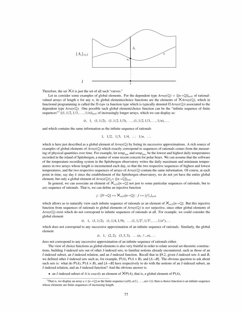
I i

Ai

a

ai•

•

Aii∈I

Therefore, the set×A is just the set of all such “curves.”Let us consider some examples of global elements. For the dependent type Array(Q) = [n→Q]n∈N of rational-

valued arrays of length n for any n, its global elements/choice functions are the elements of ×Array(Q), which infunctional programming is called the Π-type (a function type which is typically denoted Π Array(Q)) associated to thedependent type Array(Q). One possible such global element/choice function can be the “infinite sequence of finitesequences1” (1, 1/2, 1/3, . . . , 1/n)n∈N of increasingly longer arrays, which we can display as:

∅, 1, (1, 1/2), (1, 1/2, 1/3), . . . (1, 1/2, 1/3, . . . , 1/n), . . .

and which contains the same information as the infinite sequence of rationals

1, 1/2, 1/3, 1/4, . . . 1/n, . . .

which is here just described as a global element of Array(Q) by listing its successive approximations. A rich source ofexamples of global elements of Array(Q) which exactly correspond to sequences of rationals comes from the measur-ing of physical quantities over time. For example, let tempmin and tempmax be the lowest and highest daily temperaturesrecorded in the island of Spitsbergen, a matter of some recent concern for polar bears. We can assume that the softwareof the temperature recording system in the Spitsbergen observatory writes the daily maximum and minimum temper-atures in two arrays whose length is incremented each day, so that the two respective sequences of highest and lowesttemperatures, and the two respective sequences of arrays of Array(Q) contain the same information. Of course, at eachpoint in time, say day k since the establishment of the Spitsbergen observatory, we do not yet have the entire globalelement, but only a global element of Array(Q)k= [n→Q]n∈k.

In general, we can associate an element of ×n∈N[n→Q] not just to some particular sequences of rationals, but toany sequence of rationals. That is, we can define an injective function

j : [N→Q]×n∈N[n→Q] : f 7→ fnn∈N

which allows us to naturally view each infinite sequence of rationals as an element of×n∈N[n→Q]. But this injectivefunction from sequences of rationals to global elements of Array(Q) is not surjective, since other global elements ofArray(Q) exist which do not correspond to infinite sequences of rationals at all. For example, we could consider theglobal element

∅, 1, (1, 1/2), (1, 1/4, 1/9), . . . (1, 1/2n, 1/3n, . . . , 1/nn), . . .

which does not correspond to any successive approximation of an infinite sequence of rationals. Similarly, the globalelement

∅, 1, (2, 2), (3, 3, 3), . . . (n, n. . ., n), . . .

does not correspond to any successive approximation of an infinite sequence of rationals either.The view of choice functions as global elements is also very fruitful in order to relate several set-theoretic construc-

tions, building I-indexed sets out of other I-indexed sets, to familiar notions already encountered, such as those of anI-indexed subset, an I-indexed relation, and an I-indexed function. Recall that in §9.2, given I-indexed sets A and B,we defined other I-indexed sets such as, for example, P(A), P(A × B), and [A→B]. The obvious question to ask aboutsuch sets is: what do P(A), P(A × B), and [A→B] have respectively to do with the notions of an I-indexed subset, anI-indexed relation, and an I-indexed function? And the obvious answer is:

• an I-indexed subset of A is exactly an element of×P(A), that is, a global element of P(A),

1That is, we display an array a ∈ [n→Q] as the finite sequence (a(0), a(1), . . . , a(n-1)); then a choice function is an infinite sequencewhose elements are finite sequences of increasing length.

77

• an I-indexed relation from A to B is exactly an element of×P(A × B), that is, a global element of P(A × B),

• an I-indexed function from A to B is exactly an element of×[A→B], that is, a global element of [A→B].

Exercise 76 Given I-indexed sets A and B, show that there are bijections⊕(A ⊕ B) (

⊕A) ⊕ (

⊕B)

×(A × B) (×A) × (×B).

Exercise 77 Given a set X, an I-indexed set A such that A ⊆ XI , and a subset B ⊆ X, prove the following set-theoreticequality:

B ∩ (⋃

A) =⋃

(BI ∩ A).

Under the assumption that I , ∅, prove the dual equality

B ∪ (⋂

A) =⋂

(BI ∪ A).

Exercise 78 Prove that for any sets I and B the following two set-theoretic equalities hold:

1.⊕

BI = B × I

2. ×BI = [I→B]

Therefore, we can always think of a cartesian product of two sets as a special case of a disjoint union, and of thefunction set from I to B as a special case of a product of an I-indexed set. Note that Exercise 36 is a very special caseof (2).

Exercise 79 (Generalizes Exercise 30). Given an I-indexed set A, a set C, and given any I-indexed function f : A −→CI , we can define the function f :

⊕A −→ C : (ai, i) 7→ fi(ai). Prove that:

1. for each i ∈ I, ii; f = fi

2. (1) uniquely determines f , that is, any function h :⊕

A −→ C such that for each i ∈ I, ii; h = fi must necessarilysatisfy h = f .

Properties (1)–(2) are graphically expressed by the following commutative diagrams (one for each i ∈ I) of functions:

⊕A

f // C

Ai

ii

OO

fi

>>||||||||

Exercise 80 (Generalizes Exercise 29). Given an I-indexed set A, a set C, and given any I-indexed function f : CI −→

A, we can define the function f : C −→×A : c 7→ fi(c)i∈I . Prove that:

1. for each i ∈ I, f ; pi = fi

2. (1) uniquely determines f , that is, any function h : C −→×A such that for each i ∈ I, h; pi = fi must necessarilysatisfy h = f .

Properties (1)–(2) are graphically expressed by the following commutative diagrams (one for each i ∈ I) of functions:

Cf //

fi BBBBBBBB ×A

pi

Ai

Exercise 81 (Initial and Final Sets Revisited). Show that for the only ∅-indexed set id∅ we have:

1.⊕

id∅ = ∅, and

2. ×id∅ = 1.

Show, furthermore, that when we specialize Exercises 79 and 80 to the case when I = ∅, they exactly mean, respectively,that ∅ is the initial set, and that 1 is the final set. This provides a different proof of these two facts, that were alreadyproved in §5.4.

78

Exercise 82 (⊕

and × Are Functorial Constructions) (Generalizes Exercise 32). In a way totally analogous toExercise 32, we can easily check that

⊕and × are functorial constructions. Indeed, given an I-indexed function

f : A −→ B, we can use Exercise 79 to define the function⊕

f :⊕

A −→⊕

B as the unique function associated tothe I-indexed function fi; iii∈I : A −→ (⊕B)I . Applying the definition in Exercise 79 it is easy to check that for each(ai, i) ∈

⊕A we have (

⊕f )(ai, i) = ( fi(ai), i).

The dual definition for× f is obtained in the expected way by changing injections by projections and the directionof the arrows. That is,× f : ×A −→ ×B is the unique function associated according to Exercise 80 to the I-indexedfunction pi; fii∈I :×A −→ B. It is then easy to check that× f maps each aii∈I ∈×A to fi(ai)i∈I ∈×B.

Prove that⊕

and× are functorial constructions, that is, that they also preserve composition and identities. Thismeans that: (i) for any I-indexed functions

Af−→ B

g−→ C

we have (⊕

f ); (⊕

g) =⊕

( f ; g) (resp., (× f ); (×g) = ×( f ; g)); and (ii) for any I-indexed set A we have⊕

idA =

id⊕ A (resp.,×idA = id A).

10.2 The Axiom of ChoiceThe above discussion of choice functions (a.k.a. global elements) has prepared the ground for the axiom of choice(AC), an axiom with far-reaching consequences. Indeed, AC is disputed by some specialists, particularly those with aconstructivist bend of mind, who prefer to develop as much of set theory as possible without assuming it. This is thereason for the notation ZFC, which abbreviates ZF + AC, so that ZF abbreviates the axioms of Zermelo-Fraenkel settheory without AC. The statement of AC is very simple:

Any I-indexed set A = Aii∈I such that for each i ∈ I the set Ai is nonempty has a choice function.

Its precise formalization as a set theory formula is just as simple:

(AC) (∀I)(∀A : I →−→ A[I])(((∀i ∈ I) A(i) , ∅) ⇒ ×A , ∅).

At first sight, AC seems “obvious.” Why couldn’t we choose an element ai for each set Ai, if all such sets Ai arenonempty? The obvious-looking AC axiom becomes a little less obvious when we reflect on what our notion of afunction is. If we think of a function λx ∈ A. t(x) ∈ B as a precise rule to assign a given output value t(x) to each inputvalue x, then the issue becomes whether, given an arbitrary I-indexed set A = Aii∈I with all their Ai nonempty, we canalways come up with a precise and principled way (a rule in some sense) of choosing for each i ∈ I an element ai ∈ Ai.

The difficulty of always being able to come up with such a rule can be illustrated by a thought experiment dueto Bertrand Russell, which he presented in one of his books on the philosophy of mathematics [42]. Russell was 98years old when he died in 1970. Had he lived for a few more years, he might perhaps have considered re-issuing hisIntroduction to Mathematical Philosophy with a new version of his thought experiment, which originally involved amillionaire having infinitely many pairs of boots and socks. The new version, besides illustrating the issues involvedin the axiom of choice, could have also served as a morality tale, providing further illustration after the Vietnamwar (Russell and Jean-Paul Sartre organized a Vietnam War Crimes Tribunal) of what Russell felt were disastrousconsequences of American imperialism.

The revised tale might perhaps have gone as follows:

Once upon a time, in an amazing world in which, besides finite things, all kinds of infinite things existed,there lived a woman called Rimmelda. She was an infinitely vain former beauty queen, married to aninfinitely rich dictator of an infinitely poor banana republic, controlled from the shadows by an infinitelypowerful CIA. Rimmelda never wore the same dress twice: she had an infinite wardrobe, with dressesfrom the most famous fashion designers, and with an infinite number of pairs of high-heel shoes. She alsohad an infinite number of pairs of silk stockings in her wardrobe.In planning her future appearance at an infinite number of state banquets, Rimmelda wanted to set inplace a clear and unambiguous method by which, when helping her to dress, her maids would hand herfirst one shoe and a corresponding stocking, and then a second matching shoe and its correspondingmatching stocking. With so many shoes and stockings around, this was badly needed, since there hadbeen great confusion among the maids, causing embarrassing mismatches in Rimmelda’s attire at somestate banquets. Trying to solve this problem, Rimmelda run into serious difficulties, which she vaguelysuspected could be mathematical in nature. A mathematics professor from the most important universityin the country was summoned to the dictator’s palace to solve the problem. This professor was a con-structivist who had had a strict moral and mathematical upbringing. He always told the truth, and he onlyaccepted as valid functions those assignments from arguments to values that could be explicitly definedby clear and unambiguous rules. He told Rimmelda that he could provide a clear rule for the shoes: the

79

first shoe chosen should always be the left shoe in the pair; but that no such clear and unambiguous rulecould be given for the stockings, since the two stockings in each pair look exactly the same. Rimmeldawent into a fit of hysteria, and the professor was accused of secretly plotting a leftist conspiracy and wassent into prison.

In the language of I-indexed sets we can explain the professor’s inability to solve Rimmelda’s problem as follows.The infinite collection of pairs of shoes can be described as an N-indexed set Shoes = Shoesnn∈N, where Shoesn isthe n-th pair of shoes. Since each set Shoesn has exactly two elements (the left shoe and the right shoe in the pair),all sets Shoesn are nonempty. And there is indeed no problem in coming up with a well-principled choice function in×Shoes: we can, for example, follow the rule of always choosing the left shoe in each pair. The infinite collectionof pairs of stockings can also be described as an N-indexed set Stockings = Stockingsnn∈N, with Stockingsn the n-th pair of stockings. Again, since each set Stockingsn has exactly two elements, all sets Stockingsn are nonempty.However, since the two stockings in each pair are indistinguishable, there seems to be no clear way of coming up withan unambiguous method or rule for choosing one of the two stockings in each pair. That is, there seems to be no clearway of unambiguously specifying a choice function in×Stockings.

The point of this story is that AC is in some sense non-constructive, since it postulates the existence of a choicefunction in the product ×A of any I-indexed set A whose component sets are all nonempty, but provides no explicitdescription of how such a choice function can be defined. The difficulty does not come from being able to pick onestocking in a single pair of stockings: we can always do that. As shown in Exercise 84, there is no difficulty either inchoosing an element in×i∈I Ai when each of the Ai is nonempty and the index set I is finite. The problem comes whenI is infinite, since then an unambiguous rule or method for the choice should be a parametric rule, that can be appliedin a uniform way (like the rule for picking the left shoe) to an infinite number of instance cases.

The axiom of choice can be further illuminated by another, very intuitive set-theoretic property that is in factequivalent to it. Recall that, right after Exercise 25, we asked the question:

Is every surjective function a right inverse?

but postponed answering such a question until now. The right answer is that this depends on whether we adopt AC asan axiom in our set theory or not. Because, in fact, AC is equivalent to the property of every surjective function being aright inverse, as the following theorem shows.

Theorem 9 AC is equivalent to every surjective function being a right inverse.

Proof. To prove the (⇒) part, just notice that f : A →−→ B is a surjective function iff the B-indexed set f −1(b)b∈B

is such that for each b ∈ B the set f −1[b] is nonempty. By AC, the set×b∈B f −1[b] is then nonempty. But what is×b∈B f −1[b]? First notice that

⋃ f −1[b]b∈B = A. Therefore,×b∈B f −1[b] ⊆ [B→A] is just the set of all functions

g : B −→ A such that for each b ∈ B, g(b) ∈ f −1[b]. That is,×b∈B f −1[b] is precisely the set of all functions that areleft inverses to f . Since×b∈B f −1[b] is nonempty, f has a left inverse, and is therefore a right inverse, as desired.

To prove the (⇐) part, let A = Aii∈I be an I-indexed set such that for each i ∈ I we have Ai , ∅. This also impliesthat for each i ∈ I the set Ai × i , ∅. Consider now

⊕A =⋃Ai × i | i ∈ I, and define the projection function

p2 :⊕

A −→ I : (ai, i) 7→ i. Since for each i ∈ I we have Ai × i , ∅, p2 is obviously surjective, and therefore,by our assumption, a right inverse. Let g : I −→

⊕A be such that g; p2 = idI . Consider now the projection function

p1 :⊕

A −→⋃

A : (ai, i) 7→ ai. I claim that g; p1 is a choice function. Indeed, for each i ∈ I we have g(i) ∈ Ai × i,and therefore, p1(g(i)) ∈ Ai. Therefore,×A , ∅, and as a consequence AC holds.

Note that Theorem 9 gives us an alternative way, given sets A and B, of proving A B. The standard way is ofcourse to exhibit an injective function f : A B. But we now have the alternative possibility of proving A Bby exhibiting a surjective function g : B →−→ A, since by Theorem 9 this ensures the existence of a left inverse (andtherefore injective, see Exercise 25) function f : A B such that f ; g = idA.

We can gain additional insights about AC by considering an older, equivalent formulation of it, which we shall callAC′:

(AC′) For every set X there exists a function c : P(X) − ∅ −→ X, from the set of its nonempty subsets toX, such that for each A ∈ P(X) − ∅ we have c(A) ∈ A.

The term choice function was originally used, in a more restricted sense, for a function c with such a property, since itchooses for each nonempty subset of X an element in that subset.

AC and AC′ are in fact equivalent, as shown by the following:

Theorem 10 AC ⇔ AC′.

Proof. For the (⇒) direction, just observe that the identity function idP(X)−∅ : P(X) − ∅ −→ P(X) − ∅ is bijectiveand in particular surjective. Therefore, idP(X)−∅ is a (P(X)− ∅)-indexed set, which we can write in sequence notationas idP(X)−∅ = AA∈P(X)−∅. Of course, since for each A ∈ P(X)−∅ the set A is nonempty, by AC the set×idP(X)−∅ =

80

×A∈P(X)−∅A is nonempty. But since⋃

(P(X) − ∅) = X, the elements of ×A∈P(X)−∅A are precisely the functionsc : P(X) − ∅ −→ X such that for all A ∈ P(X) − ∅ we have c(A) ∈ A, that is, the “choice functions” in the morerestricted sense of AC′, and they exist by the nonemptyness of×A∈P(X)−∅A, as desired.

For the (⇐) direction, by Theorem 9 it is enough to show that AC′ implies that any surjective f : A →−→ B is a rightinverse. But since f is surjective, we have f −1[b] | b ∈ B ⊆ P(A)− ∅. Let c : P(A)− ∅ −→ A be such that for allC ∈ P(A) − ∅ we have c(C) ∈ C. Then obviously the composed function

B B−→ P(B)

f−1[ ]−→ P(A) − ∅

c−→ A

is a left inverse to f , and therefore f is a right inverse, as desired. We can use the axiom of choice to prove that for any infinite set A, N A. This agrees with our intuition that

countable infinite sets are the smallest infinite sets possible, but this intuition requires a proof.

Theorem 11 For any infinite set A, N A.

Proof. All we need to do is to define an injective function f : N A. The intuitive idea of how to define sucha function is a follows. We pick an element a0 ∈ A and define f (0) = a0, then we pick a1 ∈ A − a0 and definef (1) = a1. Likewise, we pick as(n) ∈ A − a0, . . . , an and define f (s(n)) = as(n), and so on. Since all the an are different,f is injective and we are done. However, this intuitive argument, although essentially sound, makes implicit use of bothsimple recursion and AC, and therefore needs to be developed into a complete proof. To give such a full proof we reasonas follows. We let P∞(A) ⊆ P(A) − ∅ denote the subset of all the infinite subsets of A, which is trivially nonemptysince A ∈ P∞(A). We then use a choice function c : P(A) − ∅ −→ A to define a function

smaller : P∞(A) −→ P∞(A) : X 7→ X − c(X)

which is well-defined, since if X is an infinite set, X − c(X) is also infinite (otherwise X would be finite!). Bysimple recursion this then defines a function rec(smaller, A) : N −→ P∞(A). We then define our desired f : N A : n 7→ c(rec(smaller, A)(n)). To see that f is injective, first observe that: (i) if n ≥ m, then rec(smaller, A)(n) ⊆rec(smaller, A)(m), and (ii) for each n ∈ N, f (n) ∈ rec(smaller, A)(n), and f (n) < rec(smaller, A)(s(n)). Let nown,m ∈ N, with n , m. Without loss of generality we may assume n > m. Therefore, f (m) < rec(smaller, A)(s(m)). Sincen ≥ s(m), rec(smaller, A)(n) ⊆ rec(smaller, A)(s(m)); thus , f (m) < rec(smaller, A)(n). But f (n) ∈ rec(smaller, A)(n).Hence, f (n) , f (m), as desired.

Corollary 2 (Infinite iff Dedekind-Infinite) A is infinite iff there is a proper subset B ⊂ A such that A B.

Proof. For the (⇐) part, just note that if there is a proper subset B ⊂ A such that B A, A cannot be finite; therefore Amust be infinite. For the (⇒) part, by the above theorem there is an injective function f : N A. Let B = A − f (0).The desired bijection A B is then given by the function λa ∈ A. if a ∈ A − f [N] then a else f (s( f −1(a))) fi.

The axiom of choice has many other consequences, some rather technical and many far-reaching. Let me mentionone that is very intuitive. In fact, so intuitive that one might naively think it obvious. It is called cardinal comparability(CC) and has an extremely simple formulation.

(CC) Given any two sets A and B, either A B or B A.

Yet another, extremely useful property, equivalent to AC, is the property WO stating that every set can be well-ordered.Besides its non-constructive nature, another reason why AC has a special status within ZFC is that it is independent

of the other axioms of ZF in the following precise sense: (i) no contradiction is created by adding AC to ZF; and (ii) nocontradiction is created by adding ¬AC to ZF. That is, either AC or ¬AC (but obviously not both!) can be added to ZFwithout contradiction. The proof of (i) goes back to to Goedel [18]; and that of (ii) to Fraenkel (see [47], 284–289). Infact, Fraenkel’s proof of (ii) can be viewed as a formalization of Russel’s thought experiment (Rimmelda’s story), sinceit is achieved by adding to a standard model of set theory a countable family of cardinality-2 sets, just like the familyStockings = Stockingsnn∈N.

AC was first proposed by Zermelo in 1904, together with a proof that AC⇒ WO (see [47], 139–141). This causedquite a stir due to its consequences (for example, the well-ordering of the reals) and its non-constructive nature. Asubsequent more detailed proof of the same result by Zermelo (see [47], 183–198), is very much worth reading eventoday, because it addresses very cogently the various criticisms that had been leveled against his ideas and explains whyand how AC is often used in mathematical practice. For additional discussion on the axiom of choice, its wide use inmathematics, Zorn’s Lemma, and the so-called Banach-Tarski Paradox see [27].

Exercise 83 Prove that AC is equivalent to the property that for every total relation R : A =⇒ B there exists a functionf : A −→ B such that f ⊆ R.

81

Exercise 84 Prove (without using AC) that if I is a finite set and A = Aii∈I is an I-indexed set such that for each i ∈ I,Ai , ∅, then×A , ∅. Therefore, AC is only needed for I-indexed sets such that I is infinite.

Exercise 85 Prove (using AC) that for any I-indexed set A = Aii∈I such that for each i ∈ I, Ai , ∅, the projectionfunctions pi :×A −→ Ai are surjective for all i ∈ I.

Exercise 86 In the proof of Theorem 11, the set P∞(A) of infinite subsets of A was described informally. Give a settheory formula ϕ such that P∞(A) can be formally defined as the set P∞(A) = X ∈ P(A) | ϕ using the (Sep) axiom.

Exercise 87 (The Infinite Hats Puzzle, adapted from [48]). There is a prison with a countably infinite number ofprisoners, each with a prisoner number, 0, 1, 2, . . . , n, . . . on his uniform. They have unlimited mathematical powers:they can remember mathematical objects of arbitrary cardinality and can compute (in the broad sense of the word)with such objects. Also, they can survey their infinite number of fellow prisoners when they see them, and they can talksimultaneously with all of them when in the prison yard. One day the prison guards tell them:

“Tomorrow we will place a hat on the head of each of you. The hat will be either black or white; but youwill not be able to see it; however, you will be able to see the hats that all other prisoners wear, but youwill not be able to talk to them. We will give each of you a piece of paper and a pencil where you shouldwrite your guess for the color of your own hat. If all of you, except for a finite number, guess correctly thecolor of your hat, all of you will be freed; otherwise, all of you will be executed. Today, we will let youtalk to each other for an hour in the prison yard to try to find a strategy to win in this game.”

Can the prisoners agree ahead of time on a strategy that will make them free when the following day the guards placethe hats on their heads?

Solve the same puzzle when the hats the guards place on the prisoners’ heads can have any shade of grey betweentotally black and totally white (a shade can be represented as a real number s between 0 (black) and 1 (white)). Inthis case the prisoners also have infinite precision vision: they can estimate the exact shade s of grayness of any otherprisoner’s hat just by looking.

(Hint: you may find Exercise 62 useful).

82

Chapter 11

Well-Founded Relations, andWell-Founded Induction and Recursion

A well-founded relation on a set is, by definition, a terminating relation. Such relations have an enormous importancein both computer science and in mathematics for at least three reasons: (i) they are of course crucial for terminationarguments; (ii) they vastly generalize induction on the natural numbers to induction on any well-founded relation; and(iii) they vastly generalize simple and primitive recursion to well-founded recursion, a very powerful and general formof recursion that is always guaranteed to terminate.

11.1 Well-Founded RelationsDefinition 13 Given a binary relation R ⊆ A × A, the pair (A,R) is called a well-founded relation on A iff R isterminating, that is, there is no sequence a : N −→ A such that for each n ∈ N we have an R as(n), or, pictorially, nosequence such that

a0 R a1 R a2 . . . an R as(n) . . .

Let us consider some examples. The set N can be endowed with several well founded relations, including thefollowing:

• The predecessor relation (in fact, partial function) p, with n p m ⇔ n = s(m).

• The strict order relation n > m.

• The reverse divisibility relation n vid m, where, by definition, n vid m ⇔ n , 0 ∧ (∃k ∈ N) k , 1 ∧ n = k ∗ m.

Likewise, for any set A the set List(A) =⋃

n∈N[n→A] can be endowed with a well-founded head-rest superlist order(List(A),A), where, if we denote a list a : k −→ A as a finite sequence a0 . . . ak−1, then a A b iff k > 1, and either b = a0,or b = a1 . . . ak−1.

Given any set A, the setPfin(A) of finite subsets of A can be endowed, among others, with two different well-foundedrelations. The most obvious one is (Pfin(A),⊃). Another interesting well-founded relation (indeed, a subrelation of ⊃)is the singleton-rest relation (Pfin(A),A), which is analogous to the head-rest superlist relation for lists, where, bydefinition, given X,Y ∈ Pfin(A) we have X A Y iff X has at least two elements and there exists x ∈ X such that eitherY = x, or Y = X − x. Note that the inverse relation (Pfin(A),⊂) is well-founded iff A is finite.

Yet another well-founded relation is provided by the immediate subterm relation between arithmetic expressions,which is the set1 Exp of expressions that can be formed out of a countable set of variables x, y, x′, y, . . . and of smallerexpressions t, t′, etc., by means of the following BNF-like grammar:

0 | 1 | x | (t + t′) | (t − t′) | (t ∗ t′)

The immediate subterm relation t B t′ is then defined on Exp by the defining equivalence t B t′ ⇔ (∃t′′ ∈ Exp) t =

t′ + t′′ ∨ t = t′′ + t′ ∨ t = t′ − t′′ ∨ t = t′′ − t′ ∨ t = t′ ∗ t′′ ∨ t = t′′ ∗ t′.For non-examples, note that neither (N, <), nor (Z, >), nor (Z, <), nor (R, >), nor (R, <) are well-founded.

1Properly speaking, since our set theory is built ex nihilo out of the empty set, we would need to encode these expressions, forexample with a Godel encoding of expressions as natural numbers. For the moment I will not bother with this. I will instead assumethat we are working in a variant of set theory in which atoms such as the symbols +, − and ∗, and the variables, are all allowed aselements of other sets. Then we can, for example, represent the expression (1 + (x ∗ 0)) as the tuple (+, 1, (∗, x, 0)). In §12.5 I will givea general set-theoretic construction for a set of algebraic expressions and will further discuss this matter.

83

11.1.1 Constructing Well-Founded RelationsIt is very useful to have constructions such that, if some relations on some sets are well-founded, then other relationson other sets are also well-founded.

For any set A, the relation (A,∅) is well-founded. In particular, (∅,∅) is well-founded, and for any well-founded(A,R) there is a unique relation homomorphism ∅ : (∅,∅) −→ (A,R).

One very easy way to determine that a relation (A,R) is well-founded is to find a relation homomorphism f :(A,R) −→ (B,G) to a binary relation (B,G) which is itself well-founded. If we view (A,R) as a transition system, wecan equivalently express this idea by saying that to prove that (A,R) is teminating it is enough to find a possibly simpler,terminating transition system (B,G) and a simulation map f : (A,R) −→ (B,G).

Lemma 9 Let f : (A,R) −→ (B,G) be a relation homorphism with (B,G) well-founded. Then (A,R) is well-founded.

Proof. Suppose not. Then we have a sequence a : N −→ A such that for each n ∈ N we have an R as(n). But this thenyields a sequence a; f : N −→ B such that for each n ∈ N we have f (an) G f (as(n)), contradicting the well-foundednessof (B,G).

The following are then two immediate consequencess of the above lemma:

Corollary 3 Let (B,G) be a well-founded relation. Then:

1. Any (B′,G′) with B′ ⊆ B, G′ ⊆ G, and G′ ⊆ B′ × B′ is well-founded. In particular, for any B′ ⊆ B, the binaryrelation (B′,G ∩ B′2), called the restriction of G to B′, and denoted (B′,G|B′ ) is well-founded.

2. For any function f : A −→ B, the binary relation (A, f −1(G)) is well-founded, where, by definition, a f −1(G) a′ ⇔f (a) G f (a′).

Another useful construction is the cartesian product construction. Given well-founded relations (A,R) and (B,G), itis easy to show that the relation (A×B,R×G) is well-founded, where, by definition, (a, b) R×G (a′, b′) ⇔ a Ra′ ∧ b G b′.

A second, also well-founded, relation (A × B,R Z G) can be defined on A × B, where, by definition, (a, b) R ZG (a′, b′) ⇔ (a R a′ ∧ (b = b′ ∨ b G b′)) ∨ ((a = a′ ∨ a R a′) ∧ b G b′).

Yet a third, well-founded, lexicographic relation (A × B,Lex(R,G)) can be defined on A × B, where, by definition,(a, b) Lex(R,G) (a′, b′) ⇔ a R a′ ∨ (a = a′ ∧ b G b′).

Exercise 88 Generalize the above cartesian product construction to the product of an I-indexed family of well-foundedrelations (Ai,Ri)i∈I , by showing that the binary relation (×i∈I Ai,×i∈IRi) is well-founded, where, by definition, fora, a′ ∈ ×i∈I Ai we have a×i∈IRi a′ ⇔ (∀i ∈ I) a(i) Ri a′(i). Specialize this construction to prove that, given a well-founded relation (A,R) and a set B, the function set [B→A] is well-founded by means of the relation B→R defined bythe equivalence f B→R g ⇔ (∀b ∈ B) f (b) R g(b).

Dually, it is easy to show that the disjoint union of two well-founded relations (A,R) and (B,G) yields a well-founded relation (A ⊕ B,R ⊕G), where, by definition, (x, i) R ⊕G (y, j) ⇔ (i = j = 0 ∧ x Ry) ∨ (i = j = 1 ∧ x Gy).

Exercise 89 Generalize the above disjoint union construction to the disjoint union of an I-indexed family of well-founded sets (Ai,Ri)i∈I , by showing that the binary relation (

⊕i∈I Ai,

⊕i∈I Ri) is well-founded, where, by definition,

for (a, i), (a′, i′) ∈⊕

i∈I Ai we have (a, i)⊕

i∈I Ri (a′, i′) ⇔ i = i′ ∧ a Ri a′. Specialize this construction to provethat, given a well-founded set (A,R) and another set B, the cartesian product A × B is well-founded with the relation(a, b) R × B (a, b′) ⇔ a R a′ ∧ b = b′.

Yet another very useful construction is to associate to a well-founded relation (A,R) the well founded relation(A,R+). Indeed, the following lemma has an easy proof that is left as an exercise.

Lemma 10 If (A,R) is well founded and transitive, then it is a (strict) poset. For any well-founded (A,R) the relation(A,R+) is also well-founded and is of course a strict poset. Furthermore, any relation (A,R) is well-founded iff (A,R+)is well-founded.

As an example, note that (N, >) = (N, p+).

84

11.2 Well-Founded InductionGiven a binary relation (A,R), we call an element a ∈ A R-minimal iff R[a] = ∅. The notion of R-minimality providesa very useful, alternative characterization of well-founded relations that makes a crucial use of the axiom of choice.

Theorem 12 Given a binary relation (A,R) the following are equivalent:

1. (A,R) is well-founded.

2. Any nonempty subset B ⊆ A has an R|B-minimal element.

Proof. To see (2)⇒ (1), assume that (A,R) satisfies (2) but is not well-founded. Then consider a sequence a : N −→ Asuch that for each n ∈ N we have an R as(n). The set B = an | n ∈ N is obviously nonempty, but it has no R|B-minimalelement, contradicting assumption (2).

To see (1) ⇒ (2), assume that (A,R) is well-founded and has a nonempty subset B ⊆ A with no R|B-minimalelement. This exactly means that for each x ∈ B the set R[x] ∩ B ∈ P(B) is nonempty. But by (AC′) we know thatthere is a function c : P(B) − ∅ −→ B such that for each X ∈ P(B) − ∅ we have c(X) ∈ X. This means that we candefine a function next = λx ∈ B. c(R[x] ∩ B) ∈ B, where, by construction, x R c(R[x] ∩ B). Since B is nonempty, letb ∈ B, and consider the simply recursive sequence rec(next, b) : N −→ B. By construction this sequence is such thatfor each n ∈ N we have rec(next, b)(n) R rec(next, b)(s(n)), contradicting (1).

As an immediate collorary of the above theorem we now obtain an enormously general induction principle, namely,the principle of well-founded induction.

Theorem 13 (Well-Founded Induction). For any well founded (A,R), if a subset B ⊆ A is such that for each a ∈ A ifR[a] ⊆ B then a ∈ B, then we must have B = A.

Proof. Let B ⊆ A be such that for each a ∈ A if R[a] ⊆ B then a ∈ B, and assume B , A. Then A − B is nonemptyand has an R|(A−B)-minimal element, say a. Therefore, R[a] ⊆ B. Therefore, a ∈ B, contradicting a ∈ A − B.

Given a well-founded set (A,R), we often use the above well-founded induction principle to prove formulas of theform (∀x ∈ A) P(x). Any such formula determines a subset B = x ∈ A | P(x). Obviously, (∀x ∈ A) P(x) holds iffB = A. Using well-founded induction we can prove B = A, and therefore our formula, if we can prove

(∀a ∈ A) [(∀x ∈ R[a]) P(x)]⇒ P(a).

The above induction principle is very general, and contains many other induction principles as special cases, in-cluding the following (check in detail that the mentioned induction principles are indeed special cases as claimed):

• Peano Induction. This is just the special case of well-founded induction where (A,R) = (N, p).

• Strong Induction. This is is a variant of induction on the natural numbers where for a set B ⊆ N, if we can show0 ∈ B, and that for each n ∈ N whenever n ⊆ B then n ∈ B, then we can conclude that B = N. This is just thespecial case of well-founded induction where (A,R) = (N, >).

• List Induction. To prove a property P for all lists in List(A) it is enough to show that: (i) P(∅), (ii) (∀a ∈ A) P(a)(where we view each a ∈ A as a lenght-one list), and (iii) for any list a0 . . . ak−1 with k > 1 we can provethat P(a0) and P(a1 . . . ak−1) imply P(a0 . . . ak−1). This is just the special case of well-founded induction where(A,R) = (List(A),A).

• Structural Induction. To prove a property P for all expressions in an algebraic language (arithmetic expressionsExp are a paradigmatic example, but we could consider expressions built with any other function symbols) we:(i) prove P(a) for each constant symbol a; (ii) prove P(x) for each variable x if the expressions have variables; and(iii) for each function symbol f of n arguments in our expression language and for each expression f (t1, . . . , tn)we prove that if P(t1),∧ . . . ∧ P(tn), then P( f (t1, . . . , tn)). For our arithmetic expression example this meansthat to prove that P holds for all expressions we have to prove: P(0), P(1), P(x) for all variables x, and forf ∈ +,−, ∗ that if P(t) and P(t′), then P( f (t, t′)). This is just well-founded induction where (A,R) = (Exp,B)(the generalization to expressions with other function symbols is straightforward).

Note that the “base case” is implicit in the general formulation of well-founded induction. For the natural numbersthe base case is the case n = 0. For a well-founded (A,R), any R-minimal a ∈ A provides a base case, since thenR[a] = ∅, and for B = x ∈ A | P(x) we then obviously have ∅ = R[a] ⊆ B; therefore we must prove P(a) for allR-minimal a ∈ A. For example, for (List(A),A), the A-minimal lists are the empty list ∅ and the length-one lists a ∈ A,which provide the base cases for list induction. Therefore, to inductively prove a property P for all lists, in particularwe must prove P(∅) and P(a) for each a ∈ A.

85

11.3 Well-Founded RecursionThe idea of well founded recursion is as follows. We have a well-founded set (A,R) and another set B. We then definea recursive function f : A −→ B by defining the value of f for any argument a ∈ A in terms of the value of f for“R-smaller” arguments, that is, for arguments in R[a]. Let us see some examples of this very general method to definefunctions before we formalize the general notion.

11.3.1 Examples of Well-Founded RecursionSimple recursion is a special case of this idea. We take (A,R) = (N, p). Then, given b ∈ B and f : B −→ B, we definerec( f , b) : N −→ B in terms of the values of rec( f , a) for “p-smaller” numbers. The base case is n = 0, which hasnothing p-smaller than it. So we set rec( f , b)(0) = b. In all other cases, n = s(m), so that m is the element p-smallerthan s(m), and we set rec( f , b)(s(m)) = f (rec( f , b)(m)).Primitive recursion is another special case of this idea. We take (A,R) = (N × B, p × B) (see Exercise 89). Giveng : B −→ A and f : A −→ A, we define prec( f , g) : N× B −→ A in terms of its values for p× B-smaller arguments. Thep × B-minimal elements are those of the form (0, b), for which we define prec( f , g)(0, b) = g(b). All other elements areof the form (s(n), b), whose only p × B-smaller element is (n, b), so we define prec( f , g)(s(n), b) = f (prec( f , g)(n, b)).Ackermann’s Function can also be defined by well-founded recursion. We take (A,R) = (N × N,Lex(p, p)). A :N × N −→ N is then defined in terms of its values on Lex(p, p)-smaller arguments. For (0, n) ∈ N × N we defineA(0, n) = s(n). For (s(m), 0) ∈ N × N, the Lex(p, p)-smaller arguments are all the (m, n), and we define A(s(m), 0) =

A(m, 1). Finally, for (s(m), s(n)) ∈ N × N, the Lex(p, p)-smaller arguments are all the (m, k), plus the element (s(m), n),so we can define A(s(m), s(n)) = A(m, A(s(m), n)).List Recursion works similarly to primitive recursion. Here, the well-founded relation is (List(A),A), and the A-minimal lists are ∅ and the a ∈ A. So, to define a recursive function, let us call it rec( f , g, b) : List(A) −→ B, we needto specify an element b ∈ B and functions g : A −→ B and f : B × B −→ B. Then we define rec( f , g, b) as follows: (i)rec( f , g, b)(∅) = b, (ii) for a ∈ A, rec( f , g, b)(a) = g(a), and (iii) for a list a0 . . . ak−1 with k > 1, rec( f , g, b)(a0 . . . ak−1) =

f (g(a), rec( f , g, b)(a1 . . . ak−1)). For example, suppose that B = List(C), and that we want to extend a function g :A −→ C to a function map(g) : List(A) −→ List(C) in the obvious way, that is: (i) map(g)(∅) = ∅, (ii) for a ∈ A,map(g)(a) = g(a), and (iii) for a list a0 . . . ak−1 with k > 1, map(g)(a0 . . . ak−1) = g(a) map(g)(a1 . . . ak−1). That is,map(g) = rec( · , g,∅), where · : List(C) × List(C) −→ List(C) : (a0 . . . an−1, b0 . . . bm−1) 7→ a0 . . . an−1 b0 . . . bm−1.Structural Recursion can be used to define recursive functions on algebraic expressions. We can illustrate the idea forthe case Exp of arithmetic expressions, but all generalizes to expressions with other function symbols in a straightfor-ward way. The well-founded relation is of course (Exp,B). To define a function from Exp to B by structural recursionwe need to specify: (i) elements b0, b1 ∈ B, (ii) a function g : V −→ B, where V is the set of variables in Exp, and(iii) binary functions f+, f−, f∗ ∈ [B × B→B]. Then we can define a function, let us call it rec( f , g, b) : Exp −→ B,as follows: (i) rec( f , g, b)(0) = b0, and rec( f , g, b)(1) = b1, (ii) rec( f , g, b)(x) = g(x), and (iii) for op ∈ +,−, ∗,rec( f , g, b)(op(t, t′)) = fop(rec( f , g, b)(t), rec( f , g, b)(t′)). For example, suppose that Exp are arithmetic expressions in aprogramming language, and that the variables appearing in the expressions have some assigned integer values in mem-ory (if some variables are unasigned, we may by default give them the value 0). This means that the state of the memorycan be characterized by a function g : V −→ Z. Then the evaluation function for arithmetic expressions associated tothe memory g is the function eval(g) : Exp −→ Z that in the above notation can be defined as eval(g) = rec( f , g, b)with b0 = 0, b1 = 1, and f+, f−, f∗ the functions +,−, ∗ : Z × Z −→ Z. For example, if g(x) = 3 and g(y) = 2, theneval(g)(x ∗ (x + y)) = 15.

11.3.2 Well-Founded Recursive Definitions: Step FunctionsThe above examples give us a good, informal intuition for what a well-founded recursive function looks like. But theydo not give us a mathematical model for well-founded recursive functions. Without such a mathematical model wecannot answer crucial questions such as the following: (i) what is a well-founded recursive function definition? (ii)how do we know that each such definition indeed defines a unique function and therefore makes sense? (iii) how do weknow that all functions defined by well-founded recursion terminate? This section answers question (i) by developinga very general mathematical model of well-founded recursive definitions. Questions (ii) and (iii) are then answered in§11.3.3.

In several of the examples of well-founded recursive function presented in §11.3.1 we used some linguistic de-scription of the process of defining the value of a well-founded recursive function on an argument in terms of its valueon R-smaller arguments. But since there isn’t a single well-founded relation, but an infinite number of such relations,what we need, and we do not yet have, is a precise formulation of a general method of defining well-founded recursivefunctions that will apply to any well founded relation. Furthermore, this general method should be semantic, that is,

86

involving sets and functions, as opposed to linguisitc. Indeed, it should provide the semantic basis to properly interpretany linguistic description, such as, for example, a well-founded recursive program.

Such a semantic method of defining well-founded recursive functions is provided by the notion of a step function,which is a function that contains all the information necessary to allow us to take the next step in computing our desiredfunction. Let me first illustrate this idea with an example before giving the general definition. Consider the followingprimitive recursive definition of the addition function by means of the equalities:

• 0 + m = m

• s(n) + m = s(n + m).

This is indeed a linguistic description. But what does it really say? It is obviously circular, since + is defined in termsof itself. But this circular syntactic description implicitly contains a non-circular semantic method to extend a function,so that it becomes defined on a bigger argument. It says, “if you have any two-argument function f on natural numberswhich is defined on smaller arguments, I can tell you how to extend it to a bigger argument.” For example, if f is definedon (n,m), then we can extend f to be defined on the bigger argument (s(n),m) with the value f (s(n),m) = s( f (n,m)).

How can we precisely capture this non-circular semantic method? With a function. Which function? In thisexample, the function that maps each pair ( f , (n,m)) with f any function defined on the set R[(n,m)] into the intendedvalue of its extension for the argument (n,m). Recall that in this case R is the well-founded relation p × N. Therefore,R[(0,m)] = ∅, and R[(s(n),m)] = (n,m). The function in question can then be described by the lambda expressionλ( f , (n.m)). if n = 0 then m else s( f (p(n),m) fi. What are its domain and codomain? Its codomain is obviously N.What about its domain? Here our knowldge of I-indexed sets becomes extremely useful, since we can say it in oneblow: its domain is the set

⊕(n.m)∈N×N[R[(n,m)]→N], where, as already mentioned, R = p×N. Indeed, the elements of

such a disjoint union are exactly the pairs of the form ( f , (n.m)) with f a function with domain R[(n,m)] and codomainN. This is just a special instance of the following general notion.

Definition 14 Let (A,R) be a well-founded relation and B any set. A definition of a well-founded recursive functionfrom A to B is a function of the form h :

⊕a∈A[R[a]→B] −→ B, called the step function of the recursive function thus

defined.

In what sense does a step function define a well-founded recursive function? In the following: a step functionh :⊕

a∈A[R[a]→B] −→ B defines the recursive function, let us call it rec(h), characterized by means of the definingequality

rec(h)(x) = h(rec(h)R[x], x).

Of course this is still a circular definition, but now a semantic one in terms of h, and not by some linguistic device.However, it is not at all obvious that the above equality actually defines a unique function, that such a function exists atall, or that it is terminating, although intuitively all these things seem plausible. Settling these burning issues once andforall is the goal of §11.3.3.

For the moment we can gain further empirical evidence that defining rec(h) in this way makes sense by observingthat the step function h provides a computational method to compute rec(h)(x). Let us illustrate this idea with ourprimitive recursive definition of addition by seeing how we can compute that 2 + 2 = 4. Our function h in this caseis h = λ( f , (n.m)). if n = 0 then m else s( f (p(n),m) fi. Therefore, 2 + 2 = rec(h)(2, 2) = h(rec(h)(1,2), (2, 2)) =

s(rec(h)(1, 2)) = s(h(rec(h)(0,2), (1, 2))) = s(s(rec(h)(0, 2))) = s(s(2)) = 4.To gain a little more familiarity with step functions, we can see what a step function looks like for a type of list-

recursive function considered in §11.3.1, namely, a function of the form map( f ); specifically one such function thatallows us to compute the lenght of a list. The idea is to define a function lenght on all elements of List(A) as thefunction length = map(!A) : List(A) −→ List(1), where !A is the constant function mapping each a ∈ A to 1. Notethat the set of lists List(1), with the empty list ∅ as zero element, and the function λl ∈ List(1). 1 l, that appendsone more “1” to the left of a list l, as the successor function, satisfies the Dedekind-Lawvere axiom, and therefore is amodel of the natural numbers, namely, the model corresponding to “counting with one’s fingers,” so that, for example,the number 5 is represented by the list 1 1 1 1 1. Our step function for the above length function is then of the formh :⊕

l∈List(A)[A[l]→List(1)] −→ List(1), and has the following definition by cases (which could easily be expressedby a nested if-then-else):

• h(∅,∅) = ∅

• (∀a ∈ A) h(∅, a) = 1

• for k > 1, h( f , a0 . . . ak−1) = 1 f (a1 . . . ak−1).

Let a, b ∈ A, and let us compute length(a b a b). We have, length(a b a b) = rec(h)(a b a b) = h(rec(h)a,b a b, (a b a b)) =

1 rec(h)(b a b) = 1 h(rec(h)b,a b, (b a b)) = 1 1 rec(h)(a b) = 1 1 h(rec(h)a,b, (a b)) = 1 1 1 rec(h)(b) = 1 1 1 h(∅, b) =

1 1 1 1.

87

Exercise 90 Define the appropriate step function h for Ackermann’s funtion and for the function eval(g) : Exp −→ Zevaluating arithmetic expressions with a memory g. Use the corresponding step functions to compute the value of eachof these functions on some small arguments.

Exercise 91 (Alternative definition of step functions). Given a well-founded relation (A,R) prove that there is a contain-ment

⊕a∈A[R[a]→B] ⊆ [AB] × A. Show that, instead of using a step function h :

⊕a∈A[R[a]→B] −→ B to define

a well-founded recursive function rec(h), we can always extend such a function h to a function h′ : [AB]×A −→ B, sothat h′⊕

a∈A[R[a]→B]= h, and can then equivalently define rec(h) as rec(h′) by the equality rec(h′)(x) = h′(rec(h′)R[x]

, x). Therefore, we could alternatively have defined a step function as a function h′ : [AB] × A −→ B.

11.3.3 The Well-Founded Recursion TheoremLet us come back to the three questions raised in §11.3.2: (i) what is a well-founded recursive function definition? (ii)how do we know that each such definition indeed defines a unique function and therefore makes sense? (iii) how dowe know that all functions defined by well-founded recursion terminate? The answer to question (i) is now clear: astep function. The following theorem answers questions (ii) and (iii). Note that the proof of this theorem is a natural,yet far-reaching, generalization of the same result, in Theorem 3, for the special case of simple recursion, that is, ofwell-founded recursion for the well-founded relation (N, p).

Theorem 14 (Well-Founded Recursion). Let (A,R) be a well-founded relation, and consider a step function h :⊕a∈A[R[a]→B] −→ B. Then there exists a unique function rec(h) : A −→ B, such that for all x ∈ A, the func-

tion rec(h) satisfies the equality rec(h)(x) = h(rec(h)R[x], x).

Proof. We first prove that such a function exists, and then that it is unique. Let R(h) be the set of all h-closed relations,where, by definition, a relation Q ⊆ A × B is h-closed iff for each x ∈ A, if there is a function g : R[x] −→ B suchthat g ⊆ Q, then we have (x, h(x, g)) ∈ Q. Since A × B ∈ R(h), the set R(h) is nonempty. Define rec(h) =

⋂R(h).

It is then trivial to check that rec(h) ∈ R(h). We will be done with the existence part if we prove: (i) rec(h) is total,that is, (∀x ∈ A)(∃y ∈ B) (x, y) ∈ rec(h); and (ii) rec(h) is a function; since (i) and (ii) imply that for all x ∈ A,rec(h)(x) = h(rec(h)R[x], x).

To see (i), suppose that rec(h) is not total. This means that the set X = x ∈ A | ¬(∃y ∈ B) (x, y) ∈ rec(h) isnonempty and has an R-minimal element a ∈ X. Therefore, rec(h) is total on A − X, and R[a] ⊆ (A − X). This meansthat the projection function p1 = λ(x, y) ∈ rec(h). x ∈ (A − X) is surjective. Therefore, by Theorem 9, we have afunction q : (A−X) −→ rec(h) such that q; p1 = idA−X . Therefore, g = q[A−X] ⊆ rec(h) is a function. Therefore, sinceR[a] ⊆ (A−X) and rec(h) is h-closed, we must have (a, h(a, gR[a]) ∈ rec(h), contradicting the fact rec(h) is undefinedon a. To see (ii) suppose that rec(h) is not a function. This means that the set Y = x ∈ A | (∃y, z) (x, y), (x, z) ∈rec(h) ∧ y , z is nonempty and has an R-minimal element a′ ∈ Y . Therefore, by (i), rec(h) is a function on A − Y , andR[a′] ⊆ (A − Y). But since rec(h) is h-closed, we must have (a′, h(a′, rec(h)R[a′])) ∈ rec(h), and since a′ ∈ Y , wemust have a b ∈ B with (a′, b) ∈ rec(h) ∧ b , h(a′, rec(h)R[a′]). But if we can show that rec′(h) = rec(h) − (a′, b)is h-closed, then we get a blatant contradiction of the fact that rec(h) is the smallest h-closed relation. But we can seethat rec′(h) is indeed h-closed reasoning by cases. If x = a′, then since rec′(h)R[a′]= rec(h)R[a′] is a function, thereis exactly one choice for a function g : R[a′] −→ B such that g ⊆ rec′(h), namely, g = rec′(h)R[a′], and we have(a′, h(a′, rec′(h)R[a′])) ∈ rec′(h) by the definition of rec′(h). And if x , a′, then if g : R[x] −→ B is such thatg ⊆ rec′(h), then, a fortiori, g ⊆ rec(h), and therefore (x, h(x, g)) ∈ rec(h) by rec(h) being h-closed. But since x , a′

this means that (x, h(x, g)) ∈ rec′(h), and therefore rec′(h) is h-closed, against the minimality of rec(h). Therefore, by(i) and (ii), rec(h) exists and is a total function rec(h) : A −→ B.

To prove uniqueness, suppose that there is another function, say, g, satisfying the conditions stated in the theorem.Then we must have g ∈ R(h), which forces the set-theoretic containment rec(h) ⊆ g. But this implies rec(h) = g, since,in general, given any two sets X and Y , and any two functions f , f ′ ∈ [X→Y], whenever f ⊆ f ′ we must have f = f ′.

Exercise 92 Prove that the length of the concatenation of two lists is the sum of their lengths. Since in List(1) the listconcatenation operation · becomes natural number addition, this means that, given any set A, we must show that thefunction length = map(!A) : List(A) −→ List(1), satisfies the equality:

(∀l, l′ ∈ List(A)) length(l · l′) = length(l) · length(l′).

(Hints: (i) use well-founded induction on (List(A),A); (ii) you may be more ambitious and prove the much moregeneral equality (∀l, l′ ∈ List(A)) map( f )(l · l′) = map( f )(l) · map( f )(l′) for any f : A −→ B, getting the resultfor length = map(!A) as a special case. Note that proving more general theorems is not necessarily harder: in manycases it is easier! I call this approach “generalize and conquer”).

88

Part II

Universal Algebra, Equational Logicand Term Rewriting

89

Chapter 12

Algebras

The traditional realm of algebra was the solution of polynomial equations on numerical domains such as the integersZ (the so-called Diophantine equations), the rationals Q, the reals R, and the complex numbers C. In the 20th-century,thanks to the set-theoretic notion of mathematical structure pioneered by researchers such as Richard Dedekind, thenotion of Abstract Algebra, as the study of equationally-defined set-theoretic structures with given operations, wasvigorously pursued under the leadership of researchers such as Emmy Noether (a classic textbook, gathering the ideasaround Emmy Noether and still in use today, is that of van der Waerden [45]).

Abstract Algebra greatly broadened the very notion of algebra in two ways. First, the traditional numerical domainssuch as Z, Q R, and C, were now seen as instances of more general concepts of equationally-defined algebraic struc-ture, which did not depend on any particular representation for their elements, but only on abstract sets of elements,operations on such elements, and equational properties satisfied by such operations. In this way, the integers Z wereseen as an instance of the ring algebraic structure, that is, a set R with constants 0 and 1, and with addition + andmutiplication ∗ operations satisfying the equational axioms of the theory of rings, along with other rings such asthe ring Zk of the residue classes of integers modulo k, the ring Z[x1, . . . , xn] of polynomials on n variables, and so on.Likewise, Q, R, and C were viewed as instances of the field structure, that is, a ring F together with a division operator/ , so that each nonzero element x has an inverse 1/x with x ∗ (1/x) = 1, along with other fields such as the fieldsZp, with p prime, the fields of rational functions Q(x1, . . . , xn), R(x1, . . . , xn), and C(x1, . . . , xn) (whose elements arequotients p/q with p, q polynomials and q , 0), and so on. A second way in which Abstract Algebra broadened thenotion of algebra was by considering other equationally-defined structures besides rings and fields, such as monoids,groups, modules, vector spaces, and so on. This intimately connected algebra with other areas of mathematics suchas geometry, analysis and topology in new ways, besides the already well-known connections with geometic figuresdefined as solutions of polynomal equations (the so-called algebraic varieties, such as algebraic curves or surfaces).

Universal Algebra (the seminal paper is the one by Garett Birkhoff [4]), takes one more step in this line of general-ization: why considering only the usual suspects: monoids, groups, rings, fields, modules, and vector spaces? Why notconsidering any algebraic structure defined by an arbitrary collection Σ of function symbols (called a signature), andobeying an arbitrary set E of equational axioms? And why not developing algebra in this much more general setting?That is, Universal Algebra is just Abstract Algebra brought to its full generality.

Of course, generalization never stops, so that Universal Algebra itself has been further generalized in variousdirections. One of them, which we will fully pursue in this Part II and which, as we shall see, has many applications toComputer Science, is from considering a single set of data elements (unsorted algebras) to considering a family of suchsets (many-sorted algebras), or a family of such sets but allowing subtype inclusions (order-sorted algebras). Threeother, are: (i) replacing the underlying sets by richer structures such as posets, topological spaces, sheaves, or algebraicvarieties, leading to notions such as those of an ordered algebra, a topological algebra, or an algebraic structure on asheaf or on an algebraic variety; for example, an elliptic curve is a cubic curve having a commutative group structure;(ii) allowing not only finitary operations but also infinitary ones (we have already seen examples of such algebras withinfinitary operations —namely, complete lattices and complete semi-lattices— in §7.5); and (iii) allowing operationsto be partial functions, leading to the notion of a partial algebra. Order-sorted algebras already provide quite usefulsupport for certain forms of partiality; and their generalization to algebras in membership equational logic provides fullsupport for partiality (see [36, 39]).

91

12.1 Unsorted Σ-AlgebrasUnsorted algebras are algebras with a single set of data elements. Since, as we shall see, algebras are the models oftheories in equational logic, and equational logic is a sublogic of first-order logic, we should first of all make explicitthe syntax of equational theories, so that an algebra will then be a set-theoretic interpretation of such a syntax. Asexplained in §2, the syntax of any theory in first-order logic consists of: (i) set of symbols for constants; (ii) a set offunction symbols; and (ii) a set of predicate symbols. In equational theories, however, the only predicate symbol is thebuilt-in symbol ‘=’ for equality. Therefore, we only need to specify the syntax of constants and function symbols. Thisis done by providing a so-called signature Σ specifying such symbols.

Definition 15 An unsorted signature Σ is an N-indexed family Σ = Fnn∈N, where elements f ∈ Fn are called the n-aryfunction symbols of Σ. The 0-ary symbols c ∈ F0 are called the constant symbols.

The n-ary function symbols will be interpreted in algebras as operations of n arguments. Recalling the bijectionA [1→A] : a 7→ a, explored in detail in Exercise 35, between elements of a set a ∈ A and functions a : 1 −→ A : 0 7→a, plus the fact that A0 = 1, constants are viewed as functions of zero arguments.

For example, the following signatures define the syntax of well-known algebraic structures:

• ΣDL, the signature of Dedekind-Lawvere natural numbers, has F0 = 0, F1 = s, and Fn = ∅ for n > 1.

• ΣMON , the signature of Monoids, has F0 = 1, F1 = ∅, F2 = ∗ , and Fn = ∅ for n > 2.

• ΣGP, the signature of Groups, has F0 = 1, F1 = ( )-1, F2 = ∗ , and Fn = ∅ for n > 2.

• ΣRNG, the signature of Rings, has F0 = 0, 1, F1 = - , F2 = + ∗ , and Fn = ∅ for n > 2.

• ΣFLD, the signature of Fields, has F0 = 0, 1, F1 = - , ( )-1, F2 = + ∗ , and Fn = ∅ for n > 2.

where we either list a symbol as a character or list of characters, as in s, to indicate that s will be displayed with a prefixsyntax, so that s applied to x will be denoted s(x), or if we wish to use a convenient “mix-fix” syntax display we followthe useful convention of indicating the argument positions in the syntax of each function symbol by using underbars ‘ ’as for example in ( )-1 to indicate that applied to an argument x will yield (x)-1, and + , to indicate that applied toarguments x and y will yield x + y.

A model M of an (unsorted) first-order theory is set M together with an interpretation in M for the constants,function symbols, and predicate symbols in the theory’s signature. That is, a constant c is interpreted as an elementcM ∈ M, an n-ary function symbol f is interpreted as a function fM : Mn −→ M, and an n-ary predicate symbol P isinterpreted as an n-ary relation PM ⊆ Mn. In particular, if Σ is an unsorted signature as in Definition 15 above with nopredicate symbol, such a model is called an algebra. The only vagueness left in the above, informal definition is all thistalk about “interpretation.” Can we get rid of such vagueness? That is, can we make the notion of interpretation precisein set-theoretic terms? Of course!

Definition 16 Given an unsorted signature Σ = Fnn∈N, a Σ-algebraA is an ordered pairA = (A, A), where A is theset of elements of the algebra, and A is called its structure or interpretation function, and is an N-indexed functionA = A,n : Fn −→ [An→A]n∈N.

That is, A interprets each n-ary function symbol f as a function fA : An −→ A. Implicit in the notion of unsortedΣ-algebra A = (A, A), when viewed as a special case of a model of an unsorted first-order theory, is the intepretationof the built-in equality predicate =, which is interpeted as the identity relation on A. That is, =A = idA ⊂ A2.

Note that the notion of Σ-algebra imposes no particular equational axioms on an algebra. This is not the role of Σ,which only deals with syntax. Such axioms must be explicitly specified by a set E of equations, so that an equationaltheory is then, as we will see in more detail in §13, a pair (Σ, E), with E a set of equations between expressions builtfrom the syntax of Σ and variables. For example, the theories of groups and rings are, respectively, equational theoriesof the form (ΣGP, EGP), and (ΣRNG, ERNG), where EGP is the set of equations axiomatizing the theory of groups, andERNG is the set of equations axiomatizign the theory of rings. Of course, many ΣGP-algebras do not satisfy the axiomsEGP and therefore are not groups; and many ΣRNG-algebras do not satisfy the axioms ERNG and therefore are not rings.The whole point of universal algebra is that, given a signature Σ, there can be many sets E of equations, giving rise todifferent theories (Σ, E), (Σ, E′), etc. From this point of view, Σ-algebras are the most general class of algebras possiblefor the signature Σ, that is, the class of algebras defined by the empty set of equations, i.e., by the theory (Σ,∅).

In abstract algebra books, except for vector spaces and modules, algebraic structures are typically unsorted. Forexample, ΣMON-algebras satisfying the equations EMON = x∗1 = x, 1∗ x = x, (x∗y)∗z = x∗(y∗z), are called monoids.For A any set, the set List(A) =

⋃Array(A) of lists of elements of A defined in Section 10.1 is a monoid, with ∗

interpreted as string concatenation, i.e., a1 . . . an ∗ b1 . . . bm = a1 . . . an b1 . . . bm, and 1 interpreted as the empty string ∅.Likewise, N has two obvious commutative monoid structures (i.e., monoids satisfying also x∗y = y∗ x): a multiplicativeone, where 1 is interpreted as 1 ∈ N and ∗ is interpreted as natural number multiplication ∗ : N × N −→ N, and

92

an additive one, where 1 is interpreted as 0 ∈ N and ∗ is interpreted as natural number addition + : N × N −→ N.Likewise, Z, Q, R, and C have each a multiplicative, commutative monoid structure, and an additive, commutativemonoid structure. But there is more. The just-described additive commutative monoid structures for Z, Q, R, and C,can be naturally extended to commutative group structures, by interpreting the symbol ( )-1 as the minus operation -in, respectively, Z, Q, R, and C. The additional group theory axiom not already included in the commutative monoidaxioms is: x ∗ (x-1) = 1, which in its additive interpretation takes the form: x + (-x) = 0. Furthermore, Since acommutative ring combines an additive group structure with a multiplicative monoid structure, plus the distributivityaxiom x ∗ (y + z) = (x ∗ y) + (x ∗ z), it is easy to check that Z, Q, R, and C have all a commutative ring structure. Finally,Q-0, R-0, and C-0, are also commutative multiplicative groups, with ∗ interpreted as multiplication, and with theinverse operator ( )-1 interpreted as the multiplicative inverse function 1/ in Q-0, R-0, and C-0. That is, Q, R, andC are not only commutative rings, but also commutative fields1

Of course, N has also a ΣDL-algebra structure, with 0 interpreted as 0 ∈ N, and s as the successor function s = λn ∈N. n ∪ n. Likewise, the residue classes modulo k, Zk have also a ΣDL-algebra structure, with 0 interpreted as 0 ∈ Zk,and s interpreted as the function: λn ∈ Zk. if n < (k-1) then n + 1 else 0 fi. Note that the ΣDL-algebra N actually satisfiesno equations (except the trivial one x = x), but the ΣDL-algebra Zk satisfies the equation sk(x) = 0.

Note, finally, that there is a substantial abuse of notation in all the above: one often uses the same notation, say, N,to denote both the set itself and its intended algebraic structure, and talks of the additive monoid N or the ΣDL-algebraN. Also, one often uses symbols like 0, 1, s, + , ∗ , and - , to also denote the correspondinresponding functionsin the intended algebra. This is just the customary abuse of notation in mathematics. Whenever notation is abused,by confusing data sets with algebras and function symbols with functions, one should always keep clearly in mind theessential distinction between sets and algebras; and between the syntactic level of function symbols in a signature Σ,which as such are still uninterpreted, and the semantic level of actual functions, which interpret such function symbolsin a given Σ-algebra. To be fully precise, one should use a different notation for each structure, and qualify the functionsymbols by their interpretation. For example, one could write N0,+ = (N, 0N,+N) for the additive monoid structure,and N0,s = (N, 0N, sN) for the ΣDL-algebra structure, on the set N.

Exercise 93 Let ΣDL = Fnn∈N be the Dedekind-Lawvere signature, that is, F0 = 0, F1 = s, and Fn = ∅ for n > 1.And let A = a, b, c. How many different ΣDL-algebras A = (A, A) can be defined on the set A? Can you give ageneral formula counting, for any finite set B and any unsorted signature Σ = Fnn∈N with

⋃n∈N Fn finite, how many

Σ-algebras B = (B, B) there are on B? For example, can your formula predict exactly how many such algebras willthere be on the above set A if we add to ΣDL binary function symbols + and × , so that now F2 = + , × ?

12.2 Many-Sorted Σ-AlgebrasThe passage from unsorted to many-sorted algebras is the analogue in Algebra of the passage in Computer Sciencefrom untyped programming languages to typed programming languages. This is more than an analogy since, as weshall see later, equational logic can itself be used as a programming language, which can be untyped if we adoptan unsorted equational logic, or can instead be typed using a many-sorted or order-sorted equational logic. In a many-sorted signature we allow a set S of type names2 called sorts; and then each function symbol is typed in S , by specifyingthe list of its argument sorts, and the sort of its result sort. Here is the precise definition:

Definition 17 A many-sorted signature Σ is an ordered pair Σ = (S , F), where S is called the set of sorts, and F =

Fw,s(w,s)∈List(S )×S is the (List(S ) × S )-indexed set of its function symbols.

If w = s1 . . . sn and f ∈ Fw,s, we then display f as f : s1 . . . sn −→ s, to indicate that it has argument sorts w = s1 . . . sn

and result sort s. A constant of sort s is a function symbol c ∈ F∅,s, usually denoted c : nil −→ s, since the empty string∅ is usually denoted by nil.

Note that an unsorted signature is essentially the same thing as a many-sorted signature with a singleton set ofsorts, say, S = U, where we think of U as the “universe” sort. The only notational difference between a 1-sortedsignature Σ = (U, F) and an unsorted one Σ = Fnn∈N, is that instead of denoting a function symbol f of n argumentsas f ∈ FU n...U,U we leave the universe sort U implicit and write instead f ∈ Fn.

At the level of algebras, unsorted algebras are naturally generalized to many-sorted algebras.

1Properly speaking, the theory of fields is not an equational theory, since division by 0 is undefined. We can view a field both as apartial algebra, and as a model of a non-equational first-order theory.

2Again, such type names, even if they have suggestive-sounding names such as Nat, Bool, or List, are still unintepreted names:they will be interpreted by corresponding sets in a given algebra.

93

Definition 18 For Σ = (S , F) a many-sorted signature, a many-sorted Σ-algebra is a pair A = (A, A), where A =

Ass∈S is an S -indexed set, and A, called the structure or interpretation map, is a List(S ) × S -indexed function

A = A,w,s : Fw,s −→ [Aw→As](w,s)∈List(S )×S : f 7→ fA

where, by defintion, if w = nil, then Anil = A0 = 1, if w = s : 1 −→ S : 0 7→ s, then As = As, and if w = s1 . . . sn withn > 1, then As1 ...sn = As1 × . . . × Asn .

That is, in A = (A, A), each constant symbol c : nil −→ s is interpreted as an element cA ∈ As, each f : s −→ s′

as a function fA : As −→ As′ , and each f : s1 . . . sn −→ s as a function fA : As1 × . . . × Asn −→ As′ . Therefore, amany-sorted algebra A = (A, A) is a sort-preserving interpretations of Σ, where each sort s is interpreted as a set As,and each function symbol f in F is intepreted as a function fA respecting its arity sorts and its result sort.

A well-known example of a two-sorted Σ-algebra is a vector space. The signature Σ = (S , F) has S = Scalar,Vector,and F has the function symbols: F = 0 :−→ Scalar, 1 :−→ Scalar,− : Scalar −→ Scalar, + : Scalar Scalar −→Scalar, ∗ : Scalar Scalar −→ Scalar, · : Scalar Vector −→ Vector, ~0 −→ Vector,− : Vector −→ Vector, + :Vector Vector −→ Vector. A vector space is exactly a Σ-algebra for this signature such that: (i) the set of scalars isa commutative field, (ii) the set of vectors is a commutative group, and (iii) scalar multiplication satisfies the laws:a · (v + v′) = (a · v) + (a · v′), (a + b) · v = (a · v) + (b · v), 1 · v = v, and (a ∗ b) · v = a · (b · v). For example, bychoosing R as the set of scalars with the usual addition, substraction, and multiplication operation on reals, and R3 asthe set of vectors, with vector addition (a, b, c) + (a′, b′, c′) = (a + a′, b + b′, c + c′), and with scalar multiplicationd · (a, b, c) = (d ∗ a, d ∗ b, d ∗ c), we get the usual 3-dimensional Euclidean vector space. By relaxing the requirement onscalars to be just a commutative ring instead of a field, and keeping the vectors also as an abelian group with the sameequations for scalar multiplication, we get the more general notion of a module. For example, by choosing Z as theset of scalars with the usual addition, substraction, and multiplication operation on reals, and Z3 as the set of vectors,again with the usual vector addition and scalar multiplication, we get the module of 3-dimensional vectors with integercoordinates.

Other examples of Σ-algebras can be provided by choosing a signature Σ with set of sorts S = List,Nat, and withfunction symbols nil : nil −→ List, ; : List List −→ List, 0 : nil −→ Nat, s : Nat −→ Nat, and length : List −→ Nat.Using the sort names as hints, the most “obvious” Σ-algebras are algebras interpreting Nat by N, List by List(A), for Aa set, and 0 by 0 ∈ N, s by λn ∈ N. n ∪ n, nil by nil ∈ List(A), ; as list concatenation in List(A), and length as thefunction length : List(A) −→ N which can be defined by well-founded recursion (see §11.3) by the recursive equations:length(nil) = 0, length(a) = 1 for each a ∈ A, and length(a1 a2 . . . an) = s(length(a2 . . . an)). However, as alreadymentioned, it can be misleading to take the hints given by the sort names too literally, since many other interpretationsare possible. For example, an equally natural family of Σ-algebras is obtained by interpreting Nat by N, List by P f in(A),for A a set, and 0 by 0 ∈ N, s by λn ∈ N. n ∪ n, nil by ∅ ∈ P f in(A), ; as set union in P f in(A), and length as thecardinality function | | : P f in(A) −→ N which assigns to each finite set X ∈ P f in(A) the number of its elements (formore on cardinals and the cardinality function see §§?? and ??).

12.3 Order-Sorted Σ-AlgebrasIn Computer Science one uses many different types of data. Therefore, an unsorted (usually called unyped) setting isa bad idea or, if you wish, an inferior technology: it is an unending source of silly bugs that could have been caught iftyping had been enforced by a type checker. Often, what amounts to a many-sorted type checking discipline (sometimesunder the description of a “simply typed” language) is adopted in many language designs (imperative or declarative,and in either a first-order or a higher-order setting). However, simply typed languages are not expressive enough to dealwith partiality issues, such as division by 0, or assigning a type to the head of a list l when l is empty.

An order-sorted typing discipline, in which types are arranged in type hierarchies by subtype inclusion, such as,for example, subtype inclusions Nat < Int < Rat from natural to integers and to rational numbers, and where functionsymbols can be subsort overloaded, so that, for example, addition + and multiplication ∗ can be defined for thetypes Nat, Int, and Rat is considerably more flexible than the simply typed discipline offered by many-sorted signatures.Furthermore, an order-sorted typing discipline can quite easily accomodate many often-occurring partial functions, andcan easily deal with the corresponding type exceptions caused by such functions, which become a nightmare in a simplytyped, many-sorted discipline. Common type exceptions of this kind include those caused by expressions such as: p(0),to compute the predecessor of 0, 7/0, i.e., division by zero, head(nil), i.e., trying to compute the first element of anempty list, and top(empty), i.e., trying to compute the top of an empty stack. The point is that in an order-sorted typingdiscipline all these partial functions, p, / , head, and top become total in approapriate subtypes, namely, the subtypesNzNat, of non-zero natural numbers, NzRat, of non-zero rationals, NeList, of non-empty lists, and NeStack of nonemptystacks.

This typing flexibility is further enhanced by the possibility of giving the benefit of the doubt to expressions that,although in principle meaningful, are detected at parse time to be potentially problematic. For example, it is not clear

94

at parse time which of the fractions 3/(4 + ((−3) ∗ 3)) and 3/(4 + ((−2) ∗ 2)) will have a nonzero denominator, soboth should be given the benefit of the doubt, waiting until after they are evaluated to detect type errors. Instead,the expression 3/true is utter nonsense and should be immediately rejected by a parser as meaningless. Technically,this extra typing flexibility is achieved as follows. Type names, which we always call sorts, are arranged in subsorthierarchies forming a poset (S , <), which, as a graph, may have different connected components (see Excercise 67). Togive the benefit of the doubt to meaningful expressions such as 3/(4 + ((−3) ∗ 3)) which cannot be properly typed atparse time (because the parser cannot infer that (4 + ((−3) ∗ 3) has sort NzInt), what we can do is: (i) add a fresh newsort, say >[s], strictly bigger than all sorts in each connected component3 [s] of the poset of sorts (S , <); and (ii) addfor each operator f : s1 . . . sn −→ s in Σ a new, overloaded operator f : >[s1] . . .>[sn] −→ >[s]. This is what Maude(see [10]) automatically does, denoting the “kind” >[s] by just [s]. In this way, expressions that would not parse in theoriginal signature Σ, but that are still meaningful, can be given the benefit of the doubt at parse time as expressions atthe kind level. That is, both 3/(4 + ((−3) ∗ 3)) and 3/(4 + ((−2) ∗ 2)) will be parsed as having kind [Rat]. A typingerror in the evaluation of an expression now means that the evaluated expression has a kind [s], but has no sort s in theoriginal signature Σ. For example, although the expression 3/(4+ ((−3)∗3)) evaluates to -3/5 of sort NzRat without anyproblems, the expression 3/(4 + ((−2) ∗ 2)) will evaluate to 3/0 of kind [Rat]. Therefore, having a kind but not having asort means that the corresponding functional expression is partial and is undefined for the given arguments. Note thatreturning a typing error in the form of an evaluated expression of kind [s] gives much more information than returningan “undefined” value such as ⊥.

Here is the precise definition of an order-sorted signature:

Definition 19 An order-sorted signature Σ is an ordered pair Σ = ((S , <), F) where: (i) (S , <) is a poset, called theposet of sorts, and (ii) (S , F) is a many-sorted signature.

That is, an order-sorted signature is just a many-sorted signature to which we have added a partial order relation ofsubsort inclusion between its sorts. Note that we can recover many-sorted signatures as the special case of order-sortedsignatures of the form Σ = ((S ,∅), F), that is, signatures where sorts are never related by subsort inclusion. This meansthat order-sorted signatures generalize many-sorted signatures, which, in turn, generalize unsorted signatures. And, aswe shall see shortly, the same happens for algebras: order-sorted algebras generalize many-sorted algebras, which, inturn generalize unsorted algebras. In the spirit of Universal Algebra, we should develop the relevant concepts and proveeverything at the greatest possible level of generality. Since any result about order-sorted algebras is automatically aresult about many-sorted and unsorted algebras as special cases, from now on all further developments will always becarried out at the order-sorted level.

But in this case, the drive for greater generality is not some kind of Bourbaki-like obsession: it is eminently practicalfrom the computer science point of view: why using a loser technology such as unsorted signatures and algebras whena much more expressive and useful order-sorted language technology is available? Paradoxically, it is precisely thedisregard for practical computer science applications of equational logic and term rewriting to equational specificationand programming that lies behind “vanilla flavored,” unsorted approaches that cater to theoreticians, but are impracticalfor real specification and programming.

Note that overloading of function symbols was already available in many-sorted signatures: if Σ = (S , F) is amany-sorted signature, nothing prevents the same function symbol f from having two different typings as f ∈ Fw,s,and f ∈ Fw′ ,s′ , perhaps not just with different argument and result sorts, but also with different numbers of arguments.For example, if we adopted a prefix syntax for a minus symbol - (so that the argument places are not indicated in thesyntax), we can have typings - : Int −→ Int, and - : Int Int −→ Int for unary and binary versions of -. But in a many-sorted setting such different typings are in principle unrelated in their semantic intepretation. According to Definion 18,provided we preserve type assignments, if (w, s) , (w′, s′), a many-sorted Σ-algebraA can associate any function withsuch typing, fA,w,s ∈ [Aw, As] to an f : w −→ s, and a completely different and unrelated function fA,w′ ,s′ ∈ [Aw′ , As′ ] toan f : w′ −→ s′.

Admittedly, in some particular algebras the fact that we are using the same function symbol may have a certainsignificance. For example, in the standard intepretation of the function symbols - : Int −→ Int, and - : Int Int −→ Intin Z, these two different typings of - are related by the equation: -(x, y) = x + (-y). But no relation at all need exist ingeneral. For example, we can have the following two typings of + in a many-sorted signature: + : Int Int −→ Int,and + : Bool Bool −→ Bool, and an algebra where Int is interpreted as Z, and + : Int Int −→ Int as integeraddition, and where Bool is interpreted as 2 and + : Bool Bool −→ Bool as the exclusive or function , whichis unrelated to integer addition, except for the fact that it can indeed be understood as addition in Z2. Since in priciplethere is no connection between the interpretations that can be given to two diffentent typings of a symbol f in a manysorted signature, such overloading is called ad-hoc overloading.

What about function symbol overloading in an order-sorted signature? We can still have ad-hoc overloading in acase like + : Int Int −→ Int, and + : Bool Bool −→ Bool, where there is no semantic relation between the two

3As explained in Excercice 67, the connected component of a sort s should properly denoted [s]<. It is the equivalence classassociated to s by the smallest equivalence relation < generated by <. In what follows I will abbreviate [s]< to just [s].

95

typings. But we can now also have typings like + : Nat Nat −→ Nat, and + : Rat Rat −→ Rat, which are relatedto the typing + : Int Int −→ Int in the subsort ordering Nat < Int < Rat. These second typings are an instance ofwhat is called subsort overloading of function symbols. As we shall see below, the intended semantic relation betweensubsort overloaded function symbols in an order-sorted algebra is that they should agree on common data. For example,2 + 2 should yield 4 as a result, regardless of whether we typed the + function symbol to have sort Nat, Int, or Rat.Here is the precise definition.

Definition 20 Given an order-sorted signature Σ = ((S , <), F), two typings of a function symbol f , f : s1 . . . sn −→ sand f : s′1 . . . s′m −→ s′, are called subsort-overloaded iff: (i) n = m, that is, they have the same number of arguments,includingthe case n = m = 0 where both are constants; and (ii) corresponding sorts are in the same connect components,that is, [s1] = [s′1], . . . , [sn] = [s′n], and [s] = [s′]. Otherwise, the typings f : s1 . . . sn −→ s and f : s′1 . . . s′n −→ s′ arecalled ad-hoc overloaded.

The natural question to ask at this point is: what are the semantic models for interpreting order-sorted signatures?Why, of course, order sorted algebras!

Definition 21 For Σ = ((S , <), F) an order-sorted signature, an order-sorted Σ-algebra is a many-sorted (S , F)-algebraA = (A, A) such that:

1. If s < s′, then As ⊆ As′ .

2. If a : nil −→ s and a : nil −→ s′ are two subsort-overloaded typings of a constant a in F, i.e., [s] = [s′], thenaA,nil,s(∅) = aA,nil,s′ (∅), i.e., a is interpreted as the same constant (subsort-overloaded constants coincide).

3. If f : s1 . . . sn −→ s and f : s′1 . . . s′n −→ s′ are two subsort-overloaded typings of f in F with n ≥ 1, i.e.,[si] = [s′i ], 1 ≤ i ≤ n, and [s] = [s′], then for each ~a ∈ As1 ...sn ∩ As′1 ...s

′n we have fA,s1 ...sn ,s(~a) = fA,s′1 ...s′n ,s′ (~a), that

is, subsort-overloaded operations agree on common data.

Of course, conditions (2) and (3) are equivalent to the single condition that for any two subsort-overloaded operatorsf : w −→ s and f : w′ −→ s′ in F, whenever ~a ∈ Aw ∩ Aw, then fA,w,s(~a) = fA,w′ ,s′ (~a), which is spelled out into cases(2) and (3) for the reader’s convenience.

Note that conditions (1)–(3) hold trivially for unsorted and many-sorted algebras, that is, the order-sorted algebranotion subsumes them as special cases. Therefore, from now on a Σ-algebra will always mean an order-sorted Σ-algebra.Condition (1) is entirely natural: syntactic subsort inclusions s < s′ are semantically interpreted as subset inclusionsAs ⊆ As′ on the corresponding data sets. Conditions (2) and (3) take care of the fact that both constants and functionsymbols can be subsort-overloaded, in which case the functions interpreting all these typings must agree on commondata. For example, we may have an order-sorted signature Σ = ((Nat, Int, <), F), with subsort order Nat < Int, andwith operations: F = 0 :−→ Nat, 0 :−→ Int, + : Nat Nat −→ Nat, ∗ : Nat Nat −→ Nat, + : Int Int −→ Int,− :Int −→ Int, ∗ : Int Int −→ Int. Then we can define an obvious order-sorted Σ-algebraA by interpreting the sort Natby the set N of natural numbers, the sort Int by the set Z of integers, but representing numbers in Z not as equivalenceclasses, but as n ∈ N if n is positive, and as −n if n is a nonzero negative number, which of course gives us the set-theoretic inclusion N ⊆ Z, as required by (1) for the subsort inclusion Nat < Int. Then we interpret 0, +, ∗ as zero,number addition, and number multiplication in, respectively, N and Z. Then, we have 0A,nil,Nat(∅) = 0A,nil,Nat(∅) = 0,so that (2) holds, and for any (n,m) ∈ N2 we have +A,Nat Nat,Nat(n,m) = +A,Int Nat,Int(n,m) = n +N m = n +Z m, and∗A,Nat Nat,Nat(n,m) = ∗A,Int Nat,Int(n,m) = n ∗N m = n ∗Z m. That is, addition and multiplication of two natural numbers canbe performed in either N or Z with the same result, which is condition (3).

12.4 Terms and Term AlgebrasΣ-terms are the algebraic expressions that we can form with the function symbols and constants of a given signatureΣ. In an unsorted setting, any function symbol f of n arguments can be applied to any n terms t1, . . . , tn to obtain anew term f (t1, . . . , tn). For example, we can apply the + sign to the arithmetic expressions 2 ∗ 3 and 7-9 to get thearithmetic expression (2 ∗ 3) + (7-9), which in prefix form we would write as +(∗(2, 3), -(7, 9)). However, in a many-sorted or order-sorted setting, not all terms are meaningful, so that nonsense terms such as 7 + false or nil + (2 ∗ 3)should be ruled out. The point is that in a many-sorted or order-sorted setting where S is the set of sorts, we should notdefine just a set of terms, but rather an S -indexed family of terms, so that a term t can be typed by its corresponding sorts by a typing relation t : s, and the indexed family of terms TΣ = TΣ,ss∈S is such that the elements of TΣ,s are exactlythose terms t such that t : s.

Of course, in an order-sorted setting, a term t can have several typings, since if we have t : s and a subsortrelation s < s′ in the poset of sorts (S , <), then we can also infer that t : s′. For example, when we consider subsortsNat < Int < Rat, the term (2 ∗ 3) + (7-9) obviously has sort Int, denoted (2 ∗ 3) + (7-9) : Int, but it has also sort Rat,

96

denoted (2 ∗ 3) + (7-9) : Rat, so that we can further form the fraction term ((2 ∗ 3) + (7-9))/11 : Rat. This suggestdefining the terms of an order-sorted signature Σ and the typing relation t : s simultaneously by the following inductivedefinition (note that, for simplicity, only the prefix form of a term is considered in this definition):

Definition 22 Given an order-sorted signature Σ = ((S , <), F), a Σ-term t of sort s ∈ S , denoted t : s, is a syntacticexpression that can be obtained by finite application of the following term formation rules:

1. For each f : s1 . . . sn −→ s in F, if t1 : s1, . . . , tn : sn, then f (t1, . . . , tn) : s. In particular, if a : nil −→ s is in F,then a : s.

2. If t : s and s < s′, then t : s′.

We denote by TΣ the S -indexed family of Σ-terms TΣ = TΣ,ss∈S , where, TΣ,s denotes the set of Σ-terms of sort s. Notealso that, by rule (2), if s < s′, then we necessarily have TΣ,s ⊆ TΣ,s′ .

Note that the Σ-terms in TΣ do not contain any variables: they only contain constants and other function symbols.They are sometimes called ground Σ-terms to make this fact explicit. However, the case of terms with variables, like( f (x, g(a, y)), where a is a constant and x, y are variables, is just a special case of the above definition. Given an order-sorted signature Σ = ((S , <), F), let us consider a (finite or infinite) S -indexed set of variables X = Xss∈S , where, weabbreviate x ∈ Xs by x : s, and, to avoid any syntactic confusions, we assume that: (i) if s , s′, then Xs∩Xs′ = ∅, and (ii)(⋃

X)∩ (⋃

s∈S Fnil,s) = ∅. That is, the names of the variables are all different, and they are all different from those of theconstants in F. Then we can view Σ-terms with variables in X as ground terms on the signature Σ(X) = ((S , <), F(X)),where, by definition, for any s ∈ S , (i) if w , nil then F(X)w,s = Fw,s, and (ii) F(X)nil,s = Fnil,s ∪ Xs. That is, we just addto Σ the variables in X as extra constans. Then a Σ-term with variables in X is, by definition, just a (ground) Σ(X)-term.

Given an order-sorted signature Σ, the S -indexed family of terms TΣ = TΣ,ss∈S can be endowed with a very naturalΣ-algebra structure as follows.

Definition 23 (Term Algebra). For Σ = ((S , <), F) an order-sorted signature, the term algebra TΣ = (TΣ, TΣ) is defined

by the interpretation map TΣwhich maps each f : s1 . . . sn −→ s in F to the function

fTΣ= λ(t1, . . . , tn) ∈ TΣ,s1 × . . . × TΣ,sn . f (t1, . . . , tn) ∈ TΣ,s

where if n = 0, so that s1 . . . sn = nil, (i.e., when f is a constant), then , by convention, f (∅) = f . That is, the operationfTΣ

(t1, . . . , tn) = f (t1, . . . , tn) acts on a purely syntactic way on the terms t1, . . . , tn to form the new term f (t1, . . . , tn).

Have we seen term algebras before? Yes, of course! They are just the algebras of data constructors, such asnumbers, lists, or trees (including the abstract syntax trees used in parsing) that we use all the time in computerscience. What Definition 23 makes explicit is that data types are algebras, where the algebraic operations consist onconstructing bigger data structures out of smaller ones. That is, the operations fTΣ

model exactly the concept of a(free) data constructor in data types. They are therefore very useful, since many data types can be defined as termalgebras. For example, we can represent the natural numbers as terms in Peano notation with an unsorted signatureΣNAT with a constant symbol 0 and a unary function symbol s. That is, we get a term model of the natural numbersN as the term algebra TΣNAT = (TΣ NAT , TΣ NAT ), where, say, the successor of the term s(s(0)) is precisely the termsTΣ NAT (s(s(0))) = s(s(s(0))). If, instead, we desire a term model of the natural numbers in Zermelo notation, we can usethe unsorted signature ΣNAT−Z with a constant ∅ and a unary operation .

Another interesting example is the term algebra of lists with elements in a set A, where ΣLIS T is the order-sortedsignature with sorts Elt, NeList, and List, subsort inclusions Elt < NeList < List, with Fnil,Elt = A, for A our chosen setof list elements, and with additional operations nil : nil −→ List, and a “cons” operator ; : Elt NeList −→ NeList.Then, the terms of sort List in TΣLIS T can be placed in bijective correspondence with the set List(A). For example, ifa, b, c ∈ A, then the terms a, and b have sort Elt, the terms a; b, and a; b; c; a have sort NeList, and the term nil has sortList.

Yet another example is a term model for binary trees with leaf elements in a set A, where ΣTREE is the order-sortedsignature with sorts Leaf , and Tree, subsort inclusion Leaf < Tree, with Fnil,Leaf = A, and with a binary tree constructor∧ : Tree Tree −→ Tree. Then, the terms of sort Tree in TΣTREE are exactly the binary trees with elements from A in

their leaves. For example, if a, b, c ∈ A, then the terms a, and b have sort Leaf , and (a∧b)∧ c, and (b∧ c)∧ (a∧ (b∧b))have sort Tree.

12.5 A Set-Theoretic Construction of Term AlgebrasStrictly speaking, the self-contained nature of these notes has been violated twice. Where? In the introduction of thefirst-order language of set theory in §2, and in the definition of Σ-terms in Definition 22. That is, the set of formulasin the language of set theory was defined by a context-free grammar, and the set of Σ-terms was inductively defined

97

using their signature Σ by a syntactic construction equivalent to giving a special type of context-free grammar, calleda tree regular grammar (if we allow mix-fix syntax, then sets of terms can be defined and parsed by general context-free grammars). The point, in both cases, is that it is not immediately clear in which sense the sets of expressions(formulas or terms) defined by such grammars are definable within set theory. That is, such sets have not been justifiedas set-theoretic constructions. Since inductive definitions of expressions in terms of grammars or of signatures arevery intuitive and are used all the time, probably this was not even noticeable, and was not worth remarking on whenthe violations occurred. Also, heavy use of the first-order language of set theory was essential from almost the verybeginning, because of the separation axiom. One needs to mentally bootstrap oneself somehow: self-containment isworth striving for, but may not be fully achievable within reasonable bounds; and if insisted upon to the bitter end itcan easily degenerate into pedantry.

Indeed, for the first-order language of set theory, a reasonable answer to give is that such a language providesthe meta-language in which we carry out our reasoning about sets, so that it would be quite unreasonable to requirea bootstrapping process from within set theory to justify its own metalanguage before set theory itself has even beendefined. Assuming grammars in our meta-language is a very weak assumption, without which one cannot even get off

the ground in defining a first-order theory. However, in the case of a term algebra, we are defining an algebra, that is, aparticular type of set-theoretic structure. Therefore, there is no excuse for not giving a full set-theoretic construction ofterm algebras, even if a grammar-based description is helpful and illuminating.

The question, therefore, is how to model the inductive set construction of terms in set theory (first-order formulasare a special case, using signatures with sorts Term, Variable, and Formula, with Variable < Term). Part ?? willprovide very general methods for defining sets by transfinite induction which, as shown in §??, include the inductiveconstruction of a set of terms as a special case. However, a solution to this problem not needing anything beyond thebasic set theory of Part I can be given and is the subject of this section. The key ingredient for this, more elementarysolution is implicitly contained in the answer to Exercise 72. If you did not take the hint given there and did not solveExercise 72, you missed the fun. The answer, of course, is that, given a set A, the sets [n→A] in the N-indexed setArray(A) = [n→A]n∈N all belong to the powerset P([NA]). In particular, since List(A) =

⋃Array(A), we have the

set-theoretic inclusions[n→A] ⊆ List(A) ⊆ [NA].

Given an order-sorted signature Σ = ((S , <), F), we can model terms as strings in an appropriate set of lists, anduse Theorem 6 to construct the S -indexed family of sets TΣ as a fixpoint. To avoid syntactic ambiguities, I will assumethat Σ has no ad-hoc overloading. This is a very mild assumption, since, if it does, it is very easy to rename the ad-hocoverloaded symbols so that no ad-hoc overloading remains. I will use a slightly more Spartan syntax than prefix syntax,namely, Polish notation. Therefore, a term f (t1, . . . , tn) will be displayed as the string f t1 . . . tn, where t is the Polishnotation display of t. For example, the arithmetic expression +(∗(2, 3),+(7, 9)) is displayed in Polish notation as thestring + ∗ 2 3 + 7 9. Since Σ has no ad-hoc overloading, the number of arguments of any function symbol f isuniquely determined, and this makes it easy to unambiguously reconstruct from any term f t1 . . . tn in Polish notationthe prefix term f (t1, . . . , tn). The set of strings to which all Σ-terms in Polish notation belong is obviously List(

⋃F).

But note that we need to generate not a set of terms, but an S -indexed set TΣ of such terms. This means that inour fixpoint construction of TΣ we should consider not the powerset P(List(

⋃F)), but, instead, the complete Boolean

algebra (in particular, complete lattice) [S→P(List(⋃

F))], where arbitrary sups and infs are defined pointwise, that is,given H ⊆ [S→P(List(

⋃F))], we define

∨H = λs ∈ S .

⋃h∈H h(s), and

∧H = λs ∈ S .

⋂h∈H h(s). The construction

of TΣ is then the minimal fixpoint of the functional

T : [S→P(List(⋃

F))] −→ [S→P(List(⋃

F))]

where, for h ∈ [S→P(List(⋃

F))], T is defined by the lambda expression

T = λh. λs ∈ S . h(s)∪ f t1 . . . tn ∈ List(⋃

F) | (∃s1, . . . , sn, s′ ∈ S )( f ∈ Fs1 ...sn ,s′ ∧ s′ ≤ s∧ t1 ∈ h(s1)∧ . . .∧ tn ∈ h(sn)).

That is, using Theorem 6, we define TΣ as the minimal fixpoint TΣ =∨T n(λs ∈ S . ∅) | n ∈ N.

Exercise 94 Prove in detail that T is a chain-continuous function.

It may be helpful to unpack the above fixpoint construction for a simple example, such as the unsorted signatureΣDL of the Dedekind-Lawvere natural numbers. In that case,

⋃FDL = 0, s and, since there is only one sort, T is

essentially a functional T : P(List(0, s)) −→ P(List(0, s)), and we have:

T (∅) = 0, T 2(∅) = 0, s 0, T 3(∅) = 0, s 0, s s 0, . . . ,T n+1(∅) = 0, s 0, . . . , s n. . . s 0, . . .

as expected.So far we have just defined the S -indexed set TΣ, not the term algebra TΣ. But doing this is quite easy. Just note

that for each f ∈⋃

F we have a function f : List(⋃

F) −→ List(⋃

F) : w 7→ f w, and for each n ∈ N we have the

98

n-fold append function appendn : List(⋃

F)n −→ List(⋃

F), with append0(∅) = nil, and appendn+1(w1, . . . ,wn+1) =

w1 appendn(w2, . . . ,wn+1). Then, for each f : s1 . . . sn −→ s in F, we define fTΣas the function:

fTΣ= λ(t1, . . . , tn) ∈ TΣ,s1 × . . . × TΣ,sn . f appendn(t1, . . . , tn) ∈ TΣ,s.

So we are done. There is, however, one nagging question left: how do we represent function symbols, that is, theelements of the set

⋃F in set theory? There are essentially two answers. The first answer is that, as I have already

mentioned and I further discuss in §??, one can use a set theory with atoms instead of building all sets ex nihilo fromthe empty set. Then, any desired function symbols can be assumed to be atoms, that is, basic elements of sets whichare not themselves sets. The second answer consists in explaining how to represent symbols in pure set theory. Thereare of course many ways to encode such symbols. The simplest one is perhaps an ASCII-like encoding as the one usedin any computer (digital computers, after all, operate on a very restricted fragment of pure set theory!), where the basiccharacters of an alphabet are placed in bijective correspondence with bit vectors, that is, with the set 2n for a suitablen, and then identifiers, viewed as character strings, are placed in bijective correspondence with List(2n). This will workfor any Σ with

⋃F finite or countable, modulo some “padding” to get to the smallest possible 2n.

Exercise 95 Assuming that the characters ‘(’ ‘)’ and ‘,’ are either available in a set theory with atoms or suitablyencoded in pure set theory, give alternative set-theoretic constructions for TΣ and TΣ in which terms are represented inprefix notation. Note that we no longer need to require that Σ does not have any ad-hoc overloading.

12.6 More on Order-Sorted SignaturesSome signatures may be ambiguous, so that the same term denotes two different things. This is of course a source ofconfusion which should be avoided. Consider, for example, a many-sorted signature Σ with set of sorts S = A, B,C,D,a constant symbol a : nil −→ A, and unary function symbols f : A −→ B, f : A −→ C, g : B −→ D, and g : C −→ D.This signature is ambiguous, because the term g( f (a)) denotes two different things: (i) the term obtained by firstapplying f : A −→ B to a and then applying g : B −→ D; and (ii) the term obtained by first applying f : A −→ C to aand then g : C −→ D. Of course, in other Σ-algebras we may get completely different results when applying these twodifference sequences of operations to the (interpretation of) a. Consider, for example, the Σ-algebraV = (V, V), whereVA = a, VB = b, VC = c, and VD = d, d′, and with aV = a, fV,A,B = (a, b), fV,A,C = (a, c), gV,B,D = (b, d), andgV,C,D = (c, d′). The the term g( f (a)) according to interpetation (i) (resp. (ii)) corresponds to the value d (resp. d′) inV. That is, g( f (a)) denotes two different data elements inV and therefore is intrinsically ambiguous.

Notice that, in the presence of subsort overloading, being unambiguous does not forbid the possibility of a termhaving several sorts. For example, 2 + 2 has sorts Nat, Int, and Rat, using the subsort-overloaded typings + :Nat Nat −→ Nat, + : Int Int −→ Int, and + : Rat Rat −→ Rat. Yet , 2 + 2 is a perfecly unambiguous term. Thatis, in a many-sorted signature Σ like the one given above, ambiguity will manifest itself by the presence of differentparses for a term, such as parses (i) and (ii) above. But in an order-sorted signature a term may have different parseswithout any ambiguity, provided they are all related in the subsort ordering. How can we capture this idea? I call anunambiguos order-sorted signature a sensible signature. Here is the definition.

Definition 24 An order-sorted signature Σ = ((S , <), F) is sensible iff: (i) for any constants of the form c : nil −→ s,and c : nil −→ s′, we must have [s] = [s′]; and (ii) for any function symbols with same number n of arguments, n ≥ 1,of the form f : s1 . . . sn −→ s, and f : s′1 . . . s′n −→ s′, if [s1] = [s′1], . . . , [sn] = [s′n], then we must have [s] = [s′].

Notice that condition (ii) was the one violated by our ambiguous signature, since for f : A −→ B and f : A −→ C,we have [A] = [A] = A, but [B] = B , C = [C]. Notice also that subsort overloaded constants such as0 : nil −→ Nat and 0 : nil −→ Int are allowed, but ad-hoc overloaded constants such as 0 : nil −→ Nat and0 : nil −→ Bool are forbidden by (i). However, ad-hoc overloaded function symbols like + : Nat Nat −→ Nat, and

+ : Bool Bool −→ Bool are allowed, provided (ii) is satisfied or they have different numbers of arguments. Note,finally, that subsort-overloaded symbols automatically satisfy conditions (i)–(ii), so no restriction is placed on them.Since sensibility is such a mild condition and avoids ambiguity, from now on all signatures will be assumed sensible.

As already mentioned, in an unambiguous order-sorted signature, a term t may still have different sorts. But whichsorts? Here is the answer.

Lemma 11 If Σ is sensible, for any Σ-term t, if t : s and t : s′, then [s] = [s′].Proof. We can prove this result by well-founded induction on the immediate subterm relation f (t1, . . . , tn) B ti (see§11.1). The case for constants follows by condition (i). Suppose now that f (t1, . . . , tn) : s, and f (t1, . . . , tn) : s′ with[s] , [s′]. This means that we must have f : s1 . . . sn −→ s1, and f : s′1 . . . s′n −→ s′1, with s1 ≤ s and s′1 ≤ s′, and witht1 : s1, . . . tn : sn and t1 : s′1, . . . tn : s′n. But since Σ is sensible and [s] , [s′], we must have an i, 1 ≤ i ≤ n, such that[si] , [s′i ]. which contradicts the induction hypothesis that ti : si and ti : s′i implies [si] = [s′i ].

99

Admittedly, since whenever we have t : s and s < s′ we also have t : s′, a term may have many sorts, although if Σ

is sensible all such sorts must belong to a single connected component of (S , <) by Lemma 11. But, in a sense, whenwe passed from the typing t : s to the typing t : s′ using s < s′, we lost information, since the typing t : s is moreprecise. For example, 0 : Nat is more precise than 0 : Rat, i.e., gives us more information about 0. This sugest thefollowing question: given a term t, what is the most precise information we can have about its typing? Assuming, as itis always the case in reasonable signatures, that (S , >) is a well-founded set, the most precise type information about tis the set of minimal elements in the order (S , <) of the set sorts(t) = s ∈ S | t : s. Obviously, the most informativeanswer possible about the typing of t is when the set sorts(t) has a minimum element, which is the least sort possible fort; that is, when the set of minimal elements of sorts(t) is a singleton set. We denote the least sort of t, when it exists, byls(t). It is easy to give examples of sensible signatures where some terms do no have a least sort. Perhaps the simplestis Σ with S = A, B,C, A < C, B < C and a single constant a with a : nil −→ A and a : nil −→ B. Obviously,sorts(a) = A, B,C, has two minimal elements, namely, A and B, so there is no least sort for a. The property that eachterm t has a least sort is so useful, that it deserves a name of its own.

Definition 25 A sensible signature Σ is called preregular iff for each Σ-term t ∈⋃

TΣ(X), the set sorts(t) = s ∈ S | t : shas a minimum element, denoted ls(t), where X is such that for each s ∈ S , Xs is a sigleton set,

The reason why we define the notion of preregular signature not for ground terms, but for terms over a set X ofvariables that has exactly one variable for each sort, is that we want preregularity to be preserved when we extend Σ toΣ(X); but this might fail to be the case if for some sorts s ∈ S the set TΣ,s is empty. Consider, for example, a signature Σ

with S = A, B,C, A < B, A < C and a subsort-overloaded unary function symbol with f : B −→ B and f : C −→ C.Then we have

⋃TΣ = ∅, so, every ground Σ-term trivially has a least sort. However, as soon as we add a variable x : A,

the term f (x) has two minimal typings, namely, f (x) : B, and f (x) : C, and therefore has no least sort. The need forconsidering terms with variables in Definition 25 can be avoided, so that the definition only mentions ground terms,provided Σ has nonempty sorts, where, by definition, Σ has nonempty sorts iff for each s ∈ S we have TΣ,s , ∅.

Is there a way to syntactically check that a sensible signature Σ is preregular? Indeed, there is, thanks to thefollowing characterization of preregular signatures in [21], where the notion of preregular signature was first proposedand studied.

Lemma 12 Let Σ = ((S , <), F) be a sensible signature. The the following are equivalent:

1. Σ is preregular.

2. For each w ∈ List(S ), if f ∈⋃

(w′ ,s),w′≥w, s∈S Fw′ ,s, then the set of sorts s ∈ S | ∃w′ ∈ List(S ). w′ ≥ w ∧ f ∈ Fw′ ,s

has a minimum element.

where, the order (S , >) is extended to the set List(S ) in the obvious way: s1 . . . sn ≥ s′1 . . . s′n iff si ≥ s′i , 1 ≤ i ≤ n.Proof. To see that (1) ⇒)(2), suppose (2) fails. This means that we have w ∈ List(S ) and f ∈ Fw′ ,s′ , f ∈ Fw′′ ,s′′

with w′,w′′ ≥ w, and with s′ and s′′ minimal elements in the set s ∈ S | ∃w′ ∈ List(S ). w′ ≥ w ∧ f ∈ Fw′ ,s. Letw = s1 . . . sn, n ≥ 0, then the typings f (x1 : s1, . . . xn : sn) : s′, and f (x1 : s1, . . . xn : sn) : s′′ are both least possible, soΣ is not preregular.

The proof that (2) ⇒ (1) is by well-founded indution on the immediate subterm relation. In the base case ofconstants, i.e., when w = nil, condition (2) trivially implies that each constant symbol c has a least sort. Considernow a term f (t1, . . . tn) ∈

⋃TΣ(X), where, by the induction hypothesis, ls(t1) = s1, . . . ls(tn) = sn. Then, by (2), the set

s ∈ S | ∃w′ ∈ List(S ). w′ ≥ s1 . . . sn ∧ f ∈ Fw′ ,s has a minimum element, say, s′. That is, there is an f : w′ → s′ in Σ

with w′ ≥ s1 . . . sn giving the smalles possible typing f (t1, . . . tn) : s′, that is, ls( f (t1, . . . tn)) = s′, as desired.

Exercise 96 Prove that Σ = ((S , <), F) is preregular iff Σ(X) is preregular for any S -indexed set of variables X satisfy-ing the usual requirement that: (i) if s , s′, then Xs ∩ Xs′ = ∅, and (ii) (

⋃X) ∩ (

⋃s∈S Fnil,s) = ∅.

We call a sensible signature order-sorted signature Σ = ((S , <), F) topped, iff each connected component [s] as atop element. If a signature is not topped, it is very easy to extend it to one that is so.

Definition 26 Let Σ = ((S , <), F) be a sensible order-sorted signature. Its top completion Σ> = ((S >, <>), F>) isobtained from Σ by: (i) extending (S , <) to the poset (S >, <>), where each connected component [s] in (S , <) having atop element is left unchanged, but if [s] lacks a top element, a new one, denoted >[s], is added above all elements of [s].The operations F are left unchanged, that is, for each (w, s) ∈ List(S >)×S > we have: F>w,s = Fw,s if (w, s) ∈ List(S )×S ,and F>w,s = ∅ otherwise.

Exercise 97 Let Σ = ((S , <), F) be an order-sorted signature with top completion Σ> = ((S >, <>), F>). Prove that:

1. If Σ is topped, then Σ> = Σ. In particular, (Σ>)> = Σ>.

2. For each s ∈ S we have TΣ,s = TΣ> ,s.

100

3. If [s] lacks a top element in (S , <), then, TΣ> ,>[s] =⋃

s′∈[s] TΣ,s′ .

4. If Σ is sensible, so is Σ>.

5. If Σ is preregular, so is Σ>.

Finally, as pointed out in §12.3, to give terms the benefit of the doubt it is useful to complete an order-sortedsignature Σ by adding a “kind” at the top of ech connected component (even if Σ is topped!), and overloading allfunction symbols at the kind level. In this way, any term that could eventually evaluate to a term having a sort in theoriginal signature is given the benefit of the doubt. Error or undefined terms, such as 7/0, are modeled as terms with akind which do not evaluate to a term with a sort. Let us denote by Σ be the signature thus obtained.

Definition 27 Given an order-sorted signature Σ = ((S , <), F), its kind completion Σ = ((S , <), F) is obtained fromΣ by: (i) extending (S , <) to the poset (S , <), where for each connected component [s] in (S , <) we add a new sort,denoted [s], above all sorts in [s], and (ii) for any f : s1 . . . sn −→ s in F, (n ≥ 0), we add an overloaded version of fat the kind level, f : [s1] . . . [sn] −→ [s] in F. We call a signature of the form Σ a kind-complete signature.

Exercise 98 Let Σ = ((S , <), F) be an order-sorted signature with kind completion Σ. Prove that:

1. For each s ∈ S we have TΣ,s = TΣ,s, that is no new terms are created below the kind level.

2. If Σ is sensible, so is Σ.

3. If Σ is preregular, so is Σ.

101

102

Chapter 13

Term Rewriting and Equational Logic

13.1 Terms, Equations, and Term RewritingBefore discussing equations and term rewriting, I introduce some useful concepts and notation for terms, subtems,contexts, and term replacement. Throughout I assume an order-sorted signature Σ = ((S , <), F), and its extensionΣ(X) = ((S , <), F(X)) by adding an S -sorted set of variables X. In a Σ-term f (t1, . . . , tn), the t1, . . . , tn are called itsimmediate subterms, denoted ti C f (t1, . . . , tn), 1 ≤ i ≤ n. Note that the inverse relation C-1 = B is well-founded, andwas already described and used in §11.1 for the special case of arithmetic expressions. A term u is called a subterm oft iff t B∗ u, and a proper subterm of t iff t B+ u. Note that, as an immediate consequence of Lemma 10 in §11.1, therelation B+ is also well-founded and a strict order. Given a term t ∈

⋃TΣ(X), we denote by vars(t) the set of its variables,

that is, vars(t) = x ∈⋃

X | t B∗ x. A term t may contain different occurrences of the same subterm u. For example,the subterm g(a) appears twice in the term f (b, h(g(a)), g(a)).

One way to make clear where a subterm is located is to replace such a subterm by a single hole, that is by a newconstant [] added1 to the signature Σ to indicate where the subterm u was before we removed it. For example, we canindicate the two places where g(a) occurs in f (b, h(g(a)), g(a)) by f (b, h([]), g(a)) and f (b, h(g(a)), []). A term with asingle occurrence of a hole is called a context. We write C[] to denote such a term. Given a context C[] and a term u,we can obtain a new term,2 denoted C[u], by replacing the hole [] by the term u. For example, if C[] = f (b, h([]), g(a))and u = k(b, y), then C[u] = f (b, h(k(b, y)), g(a)). Of course, if C[] is the context obtained from a term t by placinga hole [] were subterm u occurred, then we have the term identity t = C[u]. That is, we can always decompose aterm into a context and a chosen subterm, where if t = C[u], then the decomposition of t into the context-subterm pair(C[], u) is succinctly indicated by the more compact notation C[u]. For example, we have, among others, the followingdecompositions of our term f (b, h(g(a)), g(a)):

f (b, h(g(a)), g(a)) = f (b, h([g(a)]), g(a)) = f (b, h(g(a)), [g(a)]) = f (b, [h(g(a))], g(a)) = [ f (b, h(g(a)), g(a))]

where in the last decomposition the context part is the “empty context” []. This is very useful, since such decompositionsindicate where in a term we either have replaced one subterm by another, or could perfom such a replacement.

Definition 28 (Equations and Equational Theories). Given a sensible order-sorted signature Σ = ((S , <), F), a Σ-equation is an atomic formula t = t′, where t, t′ ∈

⋃TΣ(X), and where we require that t = t′ is well typed, in the

sense that there are sorts s, s′ ∈ S such that t ∈ TΣ(X),s, t′ ∈ TΣ(X),s′ , and [s] = [s′]. This is obviously less demandingthan requiring that t and t′ have a common sort; but it is equivalent to such a requirement if Σ is a topped signature.An (unconditional) equational theory is then a pair (Σ, E), with Σ a sensible order-sorted signature, and E a set ofΣ-equations.

In an equational theory (Σ, E) all equations t = t′ ∈ E are implicitly assumed to be universally quantified as

(∀x1 : s1, . . . , xn : sn) t = t′

with vars(t = t′) = x1 : s1, . . . , xn : sn, where, by definition, vars(t = t′) = vars(t) ∪ vars(t′).

1In a kind-complete order-sorted signature Σ with more than one connected component, we should add a new constant [] of kind[s] for each kind [s]. To avoid ambiguity, one can qualify the hole constant by its corresponding kind, as [][s].

2Of course, if the hole constant had kind [s], then u should have a sort in [s]. In this way, C[u] will always be a well-formedΣ-term. For example, (3 + 6) ∗ [false] is a nonsense term obtained this way, because the whole [] that it replaced has kind [Natural],but was replaced by a Boolean term in a different kind. I will assume throughout that this well-kindedness requirement is followed, sothat C[u] is always a well-formed Σ-term.

103

The proof theory of equational logic is already familiar to anybody with a high-school education from its use inelementary algebraic manipulations. That is, equational deduction is just the systematic replacement of equals by equalsusing the given equations E. For example, in algebraic manipulations of polynomials we may use ring theory equationssuch as: (1) x+y = y+x, (2) x∗y = y∗x,(3) (x+y)+z = x+(y+z), (4) x+0 = x, (5) x∗1 = x, (6) x∗(y+z) = (x∗y)+(x∗z),and so on, to prove, for example, the polynomial equality y + (z + (0 + (1 ∗ x)) = (y + z) + x by the following sequenceof replaments of equals by equals:

(‡) y + (z + [0 + (1 ∗ x)]) = y + (z + [(1 ∗ x) + 0]) = y + (z + [1 ∗ x]) = y + (z + [x ∗ 1]) = [y + (z + x)] = (y + z) + x

where I indicate at each point the subterm where an equation is applied by the corresponding term decomposition. Thefirst step has been taken applying equation (1) (in either direction), the second applying equation (4) from left to right,the third applying equation (2) in either direction, the fourth applying equation (5) from left to right, and the last stepapplying equation (3) from right to left.

We can make the above proof of equality (‡) more informative by giving a name, say ALG, to the above set (1)–(6)of equations, and indicating a proof step applying an equation from left to right by t →ALG t′, a proof step from rightto left by t ←ALG t′, and a proof step where we do not indicate the direction (that is, it might be either t →ALG t′, ort ←ALG t′ —in some special cases, like for equations (1) and (2), it may be both— and we do not specify which) byt ↔ALG t′. With this notation we obtain the more informative proof:

y+(z+[0+(1∗x)])↔ALG y+(z+[(1∗x)+0])→ALG y+(z+[1∗x])↔ALG y+(z+[x∗1])→ALG [y+(z+x)]←ALG (y+z)+x.

13.1.1 Term RewritingNote that certain equations, for example equations (4) and (5) above, have a natural use, when applied from left toright, as algebraic simplification rules. This is because their righthand side is clearly simpler, so that applying themsystematically from left to right leads to a simpler expression; that is, to a so-called simplified, or reduced form of theoriginal expression.

Even if an equation’s righthand side does not have an obviously simpler appearance, certain directions for apply-ing an equation lead to special syntact forms for fully simplified expressions that are often preferred. For example,applying equation (6) (distributivity) from left to right will lead to the standard way of displaying polynomials as sumsof products, whereas applying equation (4) (associativity of addition) will right-associate sums, which makes themmore readable than some random sum of monomials like (m1 + m2) + (m3 + (m4 + (m5))), which gets simplified tom1 + (m2(+(m3(+m4 +m5)))). Therefore, algebraic simplification produces a special type of equational proofs, called al-gebraic simplification proofs, where equations are always applied from left to right. Here is an algebraic simplificationproof with equations in ALG for a polynomial expression:

([x+0]∗(y+(z∗1)))+x′ →ALG (x∗(y+[z∗1]))+x′ →ALG [x∗(y+z)]+x′ →ALG [((x∗y)+(x∗z))+x′]→ALG (x∗y)+((x∗z)+x′)

This process of reduction, i.e., of algebraic simplification is called term rewriting. We can make this process explicitby choosing and orientation for an equation. That is, we can orient an equation t = t′ from left to right as a so-calledrewrite rule t → t′, and from right to left as the rewrite rule t′ → t. Of course, some orientations are better than others.For example, the equation x ∗ 0 = 0 has a much better orientation as a rewrite rule x ∗ 0 → 0 than as a rewrite rule0→ x∗0, not only because 0 is a simpler term than x∗0, but also because it has fewer variables. The main trouble withusing the orientation 0 → x ∗ 0 for algebraic simplification is that we have to guess what term should x be instantiatedto, since in principle there may be an infinite number of possible instantiations. For this reason, many authors rule outorientations t → t′ such that vars(t′) * vars(t). I will however not impose any restrictions on rewrite rules, althoughsuch restrictions will indeed be needed for some applications. Here are the precise definitions of rewrite rule, and of acollection of rewrite rules as a term rewriting system.

Definition 29 (Rewrite Rules and Term Rewriting Systems). Given a sensible order-sorted signature Σ = ((S , <), F), aΣ-rewrite rule is a sequent t → t′, where t, t′ ∈

⋃TΣ(X), and where we require that the rule t → t′ is well typed, in the

sense that there are sorts s, s′ ∈ S such that t ∈ TΣ(X),s, t′ ∈ TΣ(X),s′ , and [s] = [s′]. This is obviously less demandingthan requiring that t and t′ have a common sort; but it is equivalent to such a requirement if Σ is a topped signature.A term rewriting system (TRS) is then a pair (Σ,R), with Σ a sensible order-sorted signature, and R a set of Σ-rewriterules.

We should now formalize the process of term rewriting in a term rewriting system (Σ,R). The first matter thatneeds to be made precise is the notion of a rule’s instance. For example, in the last simplification step of the abovesimplification proof we have used the rule (x + y) + z → x + (y + z) by instantiating it with the substitution θ =

(x, (x ∗ y)), (y, (x ∗ z)), (z, x′), where we think of θ as a function θ : x, y, z −→ TΣRNG (x,y,z,x′). Since we are in atyped, order-sorted setting, variables have sorts, and substitutions must preserve such sorts. The general definition is asfollows:

104

Definition 30 (Substitutions). Let Σ = ((S , <), F) be a sensible order-sorted signature, and let X,Y be S -indexed setsof variables. Then a substitution θ is an S -indexed function θ = θs : Xs −→ TΣ(Y),ss∈S , mapping the variables of Xto Σ-terms with variables in Y. If X is finite, say, X = x1 : s1, . . . , xn : sn, then the S -indexed function θ can beunambiguously specified by a finite set of the form θ = (x1, t1), . . . , (xn, tn) such that ti : si, 1 ≤ i ≤ n.

Given a term t ∈⋃

TΣ(X), its instantiation by θ, denoted tθ, is defined inductively by:

1. xθ = θ(x), x ∈⋃

X

2. aθ = a for each constant a : nil −→ s in Σ

3. f (u1, . . . , uk)θ = f (u1θ, . . . , ukθ).

For example, for θ = (x, b), (y, (0 ∗ c)), we have (x + y)θ = b + (0 ∗ c), and (y ∗ x)θ = (0 ∗ c) ∗ b.

Exercise 99 (Plugging a subterm into a context as substitution instantiation). Let Σ be a sensible kind-complete sig-nature, and let [s] be one of its kinds. Let Y be an indexed set of variables, and consider the extended indexed set ofvariables Y[], where Y[],[s] = Y[s] ] [], and Y[],s′ = Ys′ otherwise. That is, Y[] is obtained from Y just by adding a singlenew variable [] of kind [s]. Call a term C ∈

⋃TΣ(Y[]) with a single occurrence of the constant [] a context with hole of

kind [s]. We typically write C as C = C[]. Let now u ∈ TΣ(Y)[s]. Prove that the term C[u] ∈⋃

TΣ(Y) obtained by pluggingu in the whole [] of C[] is exactly the instantiation C[]θ, for θ : Y[] −→ TΣ(Y) the substitution such that θ([]) = u, andθ(y) = y otherwise.

We are now ready to characterize the term rewriting relation and rewrite proofs.

Definition 31 (The Rewrite Relation and Rewrite Proofs).3 Let Σ = ((S , <), F) be a sensible, kind-complete signaturewith nonempty sorts, let (Σ,R) be a term rewriting system, and let Y = Yss∈S be an S -indexed set of variables.4 Thenan R-rewrite step is a pair (u, v), denoted u →R v, such that u ∈

⋃TΣ(Y) and there is a rewrite rule t → t′ ∈ R, a

substitution θ : vars(t → t′) −→ TΣ(Y), and a term decomposition u = C[tθ] such that v = C[t′θ], where, by definition,vars(t → t′) = vars(t) ∪ vars(t′).

Since Σ is kind-complete, if t → t′ ∈ R and u = C[tθ] : [s], then we must have v = C[t′θ] : [s], that is, →R neverproduces ill-formed terms, i.e., →R is a binary relation→R⊆ (

⋃TΣ(Y))2. Furthermore, →R is kind-preserving,5 i.e., if

u→R v, u→R w, v : s, and w : s′, then [s] = [s′].We denote by→+

R the transitive closure of→R, and by→∗R the reflexive-transitive closure of→R. A (Σ,R)-rewriteproof is, by definition, either a term t ∈

⋃TΣ(Y), witnessing a 0-step rewrite proof t →∗R t, or a sequence of R-rewrite

steps of the form t0 →R t1 →R t2 . . . tn−1 →R tn, with n ≥ 1, witnessing an n-step rewrite proof t0 →+R tn.

For example, the algebraic simplification sequence discussed earlier in this Section is a 4-step rewrite proof wit-nessing ((x+0)∗(y+(z∗1)))+ x′ →+

ALG (x∗y)+((x∗z)+ x′), where→ALG is the one-step rewrite relation associated to the

set of left-to right rewrite rules t → t′ | t = t′ ∈ ALG, which we shall later denote by−−−→ALG = t → t′ | t = t′ ∈ ALG.

13.1.2 Equational ProofsThe notion of an equational proof, that is, a sequence of steps of replacement of equals by equals using equationsE, is a trivial instance of the notion of a rewrite proof. Given an equational theory (Σ, E), all we need to do is toconsider proofs in the term rewriting system (Σ,

−→E ∪←−E ), where, by definition,

−→E is the set of left-to-right orientations

−→E = t → t′ | t = t′ ∈ E; and

←−E is the set of right-to-left orientations

←−E = t′ → t | t = t′ ∈ E.

3To simplify the exposition I am assuming a sensible order-sorted signature Σ that is kind-complete (see Def. 27). This assumptionsallows a considerably simpler treatment of term rewriting because, thanks to kind completeness, a rewrite step can never result in a non-well-formed term. Since any order-sorted signature Σ can be naturally extended to a kind-complete one, in practice this assumptiondoes not entail any real loss of generality. I also assume that Σ has nonempty sorts, since this avoids the need for introducing explicitquantifiers.

4For generality’s sake, I will assume that Y has a countably infinite set of variables Ys for each s ∈ S , that is, there is a bijectiveS -indexed function α : Y −→ NS ; but this requirement is not essential: any S -indexed set of variables Y can be used. That is, therelation→R is in fact parameterized by the chosen family of variables Y .

5For→R to be kind-preserving, the assumption that Σ is sensible is crucial, since this ensures Lemma 11. For a simple counterex-ample, consider Σ with sorts A, B, and C, with corresponding constant symbols a, b, c, and f : A −→ B, f : A −→ C, and R with rules:f (x : A)→ b and f (x : A)→ c. Then we have f (a)→R b, and f (a)→R c, but [B] , [C].

105

Definition 32 (The Equality Relation and Equational Proofs).6 Let (Σ, E) be an equational theory with Σ = ((S , <), F)a sensible, kind-complete signature with nonempty sorts, and Y an S -indexed set of variables7 Then an E-equality stepis, by definition, a (

−→E ∪←−E )-rewrite step u→(

−→E∪←−E ) v, denoted u↔E v, where u, v ∈

⋃TΣ(Y).

We denote by↔+E the transitive closure of↔E; and by↔∗E the reflexive-transitive closure of↔E . ↔∗E is called the

E-equality relation, and is often abbreviated to =E . It is also called the relation of equality modulo E.A (Σ, E)-equality proof is by, definition, either a term t ∈

⋃TΣ(Y), witnessing a 0-step E-equality proof t ↔∗E t, or a

sequence of E-equality steps of the form t0 ↔E t1 ↔E t2 . . . tn−1 ↔E tn, with n ≥ 1, witnessing an n-step equality prooft0 ↔

+E tn.

For example, the sequence of equality steps (‡) discussed earlier in §13.1 is a 5-step equality proof witnessingy + (z + (0 + (1 ∗ x)))↔+

ALG (y + z) + x.Notational Convention. Since in many applications a set of equations E will always be used from left to right, we shalloften abbreviate the rewrite relations→−→E ,→+

−→E

, and→∗−→E

, associated to the term rewriting system (Σ,−→E ) by, respectively,

→E ,→+E , and→∗E . Likewise, we will abbreviate the rewrite relations→←−E ,→+

←−E

, and→∗←−E

, associated to the term rewriting

system (Σ,←−E ) by, respectively,←E ,←+

E , and←∗E .

Exercise 100 The theory of groups has an unsorted signature with a constant 1, a unary function ( )−1 and a binaryfunction and has the following equations G:

• x 1 = x

• x (y z) = (x y) z

• x (x)−1 = 1

Give G-equality proofs in the sense of Definition 32 for the following theorems of Group Theory:

• 1 x = x

• (x)−1 x = 1

• (x y)−1 = y−1 x−1

(Hint: if you prove any of those theorems, then you can use them as lemmas to prove some of the others.)

Exercise 101 Prove that the E-equality relation =E defines an equivalence relation on⋃

TΣ(Y), and also on TΣ(Y),[s] foreach kind [s] ∈ S/<.

Prove also that, under the assumptions of Definition 32, =E does not depend on the set Y of variables, chosen todefine the equality relation =E . That is, given any two S -indexed sets of variables Z, Y with Z ⊆ Y, we have in fact twoequality relations, which should be notationally distinguished as =Z

E⊆ (⋃

TΣ(Z))2, and =YE⊆ (⋃

TΣ(Y))2. You are asked toprove that for any terms u, v ∈

⋃TΣ(Z) we have u =Z

E v iff u =YE v. The requirement that Σ has nonempty sorts is essential

for this to be the case, even in the many-sorted case. That is, there are signatures Σ and equational theories (Σ, E) suchthat there are S -indexed sets of variables Z ⊆ Y and terms u, v ∈

⋃TΣ(Z) such that u ,Z

E v, but u =YE v (see, [38, 20]).

13.2 Term Rewriting and Equational Reasoning Modulo AxiomsCertain equations are intrinsically problematic for term rewriting. Consider, for example, the commutativity equationsx + y = y + x, and x ∗ y = y ∗ x. Since the idea of term rewriting is to simplify a term to hopefully get a fully simplified,equivalent term, a commutativity equation is intrinsically problematic for two reasons: (i) applying a commutativityequation we do not obtain a simpler term, but only a “mirror image” of the original term; for example, (x ∗ 7) + (0 ∗ y)is rewritten by the commutativity equation to its mirror image (0 ∗ y) + (x ∗ 7); and (ii) even worse, we can loop whenapplying such equations, never reaching a fully simplified term, as in the infinite, alternating sequence

(x ∗ 7) + (0 ∗ y)→ALG (0 ∗ y) + (x ∗ 7)→ALG (x ∗ 7) + (0 ∗ y)→ALG (0 ∗ y) + (x ∗ 7)→ALG . . .

6To simplify the exposition I am assuming a sensible order-sorted signature Σ that is kind complete and has nonempty sorts (see§12.6). These two assumptions allow a considerably simpler treatment because: (i) no explicit use of universal quantifiers is needed(thanks to the nonempty sorts); and (ii) the replacement of equals by equals can never result in a non-well-formed term (thanks to kindcompleteness). If Σ has some empty sorts, a treatment with explicitly quantified equations (∀x1 : s1, . . . , xn : sn) t = t′ is needed;and if it is not kind complete, care must be taken not to generate non-well-formed terms (see, e.g., [36]). The fact that the presence ofempty sorts requires an explicit treatment of universal quantifiers in order to have a sound (and of course complete) inference systemfor equational deduction is well-known, even for many-sorted equational logic, since [38, 20].

7Again, with a countably infinite set of variables for each sort s ∈ S for generality’s sake, although this requirement is not essential:any S -indexed set Y can be used.

106

Of course, this does not block us, humans, from simplifying the above polynomial to (7 ∗ x). But a standard imple-mentation of term rewriting can easily loop when commutativity equations are used as rewrite rules. The solution tothis problem, provided by many symbolic algebra systems, and by equational programming languages such as OBJ3[22], ASF+SDF [46], CafeOBJ [17], ELAN [6], and Maude [10], is to build in certain, commonly occurring equationalaxioms, such as the above commutativity axioms, so that rewriting takes place modulo such axioms. For example, wecan decompose our equations ALG into a built-in, commutative part C = x + y = y + x, x ∗ y = y ∗ x and the rest, say,ALG0 = (x + y) + z = x + (y + z), x + 0 = x, x ∗ 1 = x, x ∗ (y + z) = (x ∗ y) + (x ∗ z), and then rewrite with the equationsin ALG0 from left to right applying them, not just to a given term t, but to any other term t′ which is provably equal to tby the equations C, that is, any t′ such that t =C t′. This, more powerful rewrite relation is called rewriting modulo C,and is denoted→ALG0/C . For example, we can simplify the expression ((0 + x) ∗ ((1 ∗ y) + 7)) + z to (x ∗ y) + ((x ∗ 7) + z)in just four steps of rewriting with→ALG0/C as follows:

((0+ x)∗((1∗y)+7))+z→ALG0/C (x∗((1∗y)+7))+z→ALG0/C (x∗(y+7))+z→ALG0/C ((x∗y)+(x∗7))+z→ALG0/C (x∗y)+((x∗7)+z)

What rewriting modulo axioms such as C achieves is raising the level of abstraction at which we simplify expressions,bringing it closer to the human level. The point is that, since equality modulo a set of axioms like C is an equivalencerelation (see Exercise 101), rewriting with →ALG0/C achieves the effect of rewriting not just terms, but C-equivalenceclasses of terms.

But why stopping with commutativity? How about associativity? An associativity equation such as (x + y) + z =

x + (y + z) does certainly not have any looping problems; but parentheses around associative operators are a nuisancethat can block the application of equations which can “obviously” be applied by humans. For example, the equationx + −x = 0 can be applied modulo associativity and commutativity to the expression ((x + y) + z) + −(y + (z + x))in one step of rewriting modulo the following set AC of associativity and commutativity axioms for + and ∗ ,AC = x + y = y + x, x ∗ y = y ∗ x, (x + y) + z = x + (y + z), (x ∗ y) ∗ z = x ∗ (y ∗ z), using from left to right the set ofequations ALG1 = x + 0 = x, x ∗ 1 = x, x ∗ (y + z) = (x ∗ y) + (x ∗ z), x + −x = 0, to the fully simplified form:

((x + y) + z) + −(y + (z + x))→ALG1/AC 0.

That is, when rewriting modulo AC: (i) the order of the arguments does not matter (because of commutativity, C),and (ii) parentheses do not matter (because of associativity, A). In fact, when rewriting modulo associativity (A), orassociativity-commutativity (AC), we can disregard parentheses altogether, and write an expression like ((x+y)+ z)+ x′

without such parentheses as x + y + z + x′, as it is standard practice in mathematics textbooks.Likewise, we could also build in the unit element axioms U = x + 0 = x, x ∗ 1 = x. Or any combination of C,

and/or A, and/or U axioms could be built in. In fact, the idea of building in a set B of equational axioms, so that werewrite with a set of rules R modulo B, is entirely general, and is captured by the notion of a rewrite theory.

Definition 33 Let Σ be a sensible order-sorted signature. A rewrite theory8

is a triple (Σ, B,R), where B is a set of Σ-equations, and R is a set of Σ-rewrite rules.

Rewriting with R modulo B can then be formalized as follows.

Definition 34 (Rewriting and Rewrite Proofs Modulo B). Let (Σ, B,R) be a rewrite theory such that Σ is sensible andkind-complete. Then an R-rewrite step modulo B is a pair (u, v) ∈ T 2

Σ(Y), denoted u →R/B v, such that there are termsu′, v′ ∈ TΣ(Y) with u =B u′, u′ →R v′, and v′ =B v, that is, we have u =B u′ →R v′ =B v. We call →R/B the one-stepR-rewrite relation modulo B, and denote by →0

R/B the relation =B, called the 0-step R-rewrite relation modulo B, by→+

R/B the transitive closure of→R/B, and by→∗R/B the relation9 →+R/B ∪ =B.

An R-rewrite proof modulo B is either: (i) a pair (u, v) ∈ T 2Σ(Y), with u =B v, witnessing a 0-step R-rewrite modulo B

proof, or (ii) a sequence of R-rewrite steps modulo B of the form v0 →R/B v1 →R/B v2 . . . vn−1 →R/B vn, n ≥ 1, witnessingan n-step proof v0 →

+R/B vn.

8The traditional use of rewriting modulo axioms has been to reason efficiently, and at a high level of abstraction, in an equationaltheory (Σ, E ∪ B) where the equations E are applied from left to right as rewrite rules modulo B. This is the main use we will makeof rewrite theories (Σ, B,R) in these notes; that is, to perform simplification modulo B in the equational theory (Σ, B ∪ eq(R)), whereeq(R) are the equations associated to the rules R. However, in rewriting logic [35, 37], a rewrite theory (Σ, E,R), has (Σ, E) as itsunderlying equational theory, but the rules R are not interpreted as equations at all, but as concurrent transitions in a concurren system,whose states are axiomatized as E-equivalence classes of terms. Futhermore, the equations E in the equational theory (Σ, E) typicallydecompose as a disjoint union G ∪ B, where the equations G can be used as simplification rules modulo B; that is, in a simpler rewritetheory (Σ, B, ~G) used for efficient equational reasoning, as the ones we will consider here. In the Maude language [10], both equationaltheories of the form (Σ, B ∪ G), called functional modules, and rewrite theories of the general form (Σ,G ∪ B,R) with a concurrentsystem semantics, called system modules are executed by rewriting with two different rewrite relations, namely,→G/B for equationalsimplification, and→R/B for concurrent transitions. Maude’s functional modules are further discusses in §??.

9Note that, in general, →∗R/B does not coincide with the reflexive-transitive closure of →R/B, but only contains it. It should bethought of as the reflexive-transitive closure of→R/B modulo B.

107

A term u ∈⋃

TΣ(Y) is said to be in R/B-normal form iff (@u′). u →R/B u′, that is, iff u cannot be further rewrittenwith R modulo B. Also, given a term t ∈

⋃TΣ(Y), we say that u is a R/B-normal form of t iff t →∗R/B u, and u is in

R/B-normal form, which we abbreviate to t →!R/B u.

Exercise 102 (Deconstructing Rewriting Modulo). What rewriting modulo B accomplishes is to raise the level ofabstraction by “building in” B-equality proofs. This suggests that, at the heavy price of losing the higher level ofabstraction thus gained, we can “deconstruct” a rewrite theory (Σ, B,R) into a semantically equivalent term rewritingsystem (Σ,R ∪

−→B ∪←−B), were we now make explicit each single step of B-equality. But is this true? Prove that if Σ is

sensible and kind-complete, then for any two Σ-terms t, t′ ∈⋃

TΣ(Y) we have t →∗R/B t′ iff t →∗R∪−→B∪←−B

t′.

Exercise 103 (Equational reasoning modulo axioms). Consider an equational theory of the form (Σ, E ] B) with Σ

sensible and kind-complete. Then we can consider the rewrite theory (Σ, B,−→E ∪←−E ), and abbreviate the rewrite relation

→−→E∪←−E/B to just↔E/B. This captures the idea of doing equational reasoning with E modulo the axioms B, which is what

we humans do when performing algebraic reasoning, and what smart implementations of equational reasoning do aswell. But is it correct? Prove that for any Σ(Y)-terms t, t′ we have the equivalence:

t =E]B t′ ⇔ t ↔∗E/B t′.

(Hint: use Exercise 102).

13.3 Sort-Decreasingness, Confluence, and TerminationGiven a rewrite theory (Σ, B,R), which executabilty conditions should be placed in practice on the rules R so that wecan effectively use it for equational simplification modulo B in the associated equational theory (Σ, B∪ eq(R)), in whichthe rules t → t′ ∈ R are now understood as equations t = t′ ∈ eq(R)?

As already mentioned for the example of the problematic rule 0→ x ∗ 0 associated to the equation x ∗ 0 = 0 whenoriented from right to left, the most basic requirement is:

(1) for each t → t′ ∈ R, any variable x occuring in t′ must also occur in t.

Otherwise, t → t′ is problematic as a rewrite rule, since we have to guess how to instantiate the extra variables in t′, andthere can be an infinity of guesses. For example, if we tried to use the rule 0→ x∗0 to “simplify” the term (a+b)+0,wecould obtain (a+b)+ (0∗0), or (a+b)+ (z∗0), or (a+b)+ ((c∗d)∗0), and so on, depending on whether the substitutionwe chose was θ = (x, 0), or θ = (x, z), or θ = (x, (c ∗ d)), and so on. Instead, if we apply the equation x + 0 = x tothe same term, there is only one substitution possible to simplify (a + b) + 0, namely, θ = (x, (a + b). Note that, underassumption (1), if u→R v, then no new variables are introduced in v; that is, we always have vars(v) ⊆ vars(u).

The additional requirement that Σ is preregular is also very useful for efficient rewriting. This is because, for arewrite step C[tθ] → C[t′θ] with a rule t → t′ in R to be legal, we need to check that θ is well-sorted; that is, that foreach (x : s, u) ∈ θ we indeed have u : s. But for Σ preregular this just becomes the easy syntactic check ls(u) ≤ s.

A second important requirement is:

(2) sort-decreasingness, that is, for each t → t′ ∈ R, sort s ∈ S , and substitution θ we should have theimplication tθ : s ⇒ t′θ : s.

It is then easy to check by well-founded induction on the context C below which a rewrite C[tθ]→R C[t′θ] takes place,that under condition (2) the rewrite relation →R preserves sorts, that is, if u →R v, then u : s ⇒ v : s. This is ofcourse always the case for unsorted or many-sorted rewriting, but it can fail to hold for order-sorted rewrite theoriesand, unless the signature Σ is kind-complete, can lead to non-well-formed terms. Consider, for example, a subsortinclusion Nat < Set, where Nat has operators 0 and s, and Set has a set union operator ∪ , that is, we view eachnatural number n as a singleton set. Then the rule x→ x ∪ x with x of sort Set fails to be sort-decreasing, since, for n avariable of sort Nat, the substitution θ = (x, n) is such that n : Nat, but n ∪ n does not have sort Nat. This does indeedlead to ill-formed tems, since we then have the rewrite s[0] → s[0 ∪ 0], where the term s(0 ∪ 0) is not a well-formedterm, unless the signature is kind-complete, so that both s and ∪ are lifted to the kind [Set]. Sort decreasingness isan easily checkable condition, since we do not need to check it on the, in general infinite, set of all substitutions θ: ifx1 : s1, . . . , xn : sn = vars(t → t′), we only need to check it on the, typically finite, set of substitutions of the form(x1 : s1, x′1 : s′1), . . . , (xn : sn, x′n : s′n) with s′i ≤ si, 1 ≤ i ≤ n, which are called the sort specializations [16] of theset of variables x1 : s1, . . . , xn : sn. For example, for the above rule x → x ∪ x, the failure was detected for the sortspecialization (x : Set, x′ : Nat), which was abbreviated to θ = (x, n).

Exercise 104 Let (Σ,R) be a term-rewriting system with Σ preregular. Prove that the rules R are sort decreasing iff foreach sort specialization ρ as defined above and for each t → t′ in R we have: ls(tρ) ≥ ls(t′ρ).

108

To see why things can go wrong when sorts are not preserved by rewriting; that is, when the rules are not sort-decreasing, consider the following simple example. There are two sorts C and D with C < D, a constant c of sortC, a constant d of sort D, and a subsort-overloaded unary function f : C −→ C, f : D −→ D. Let B = ∅ andR = c → d, f ( f (x : C)) → f (x : C). Now consider the term f ( f (c)). Using the second rule we can rewrite it to f (c),which can be further rewritten to f (d) with the first rule. But if we apply the first rule to f ( f (c)) we get f ( f (d)) whichcannot be further rewritten! The point is that the rule c→ d is not sort-decreasing, so the information that c had sort Chas been lost, and now we are stuck with f ( f (d)), since we cannot apply the second rule.

A third requirement is one of determinism: if a term t is simplified by R modulo B to two different terms u andv, and u ,B v, then u and v can always be further simplified by R modulo E to a common term w. This implies (seeExercise 105 below) that if t →∗R/B u and t →∗R/B v, and u and v cannot be further simplified by R modulo B, then wemust have u =B v. This is the idea of determinism: if rewriting with R modulo B yields a fully simplified answer, thenthat answer must be unique modulo B. That is, the final result of a reduction with the rules R modulo B should notdepend on the order of evaluation, i.e., on the particular order in which the rewrites have been performed in the rewritesequence. This is precisely captured by the requirement of confluence below. Note that, since the relation u→∗R v is justthe special case of the relation u→∗R/B v in which B = ∅, confluence of R is a special case of confuence of R modulo B.

Definition 35 Let (Σ, B,R) be a rewrite theory. Then the rules R are called confluent modulo B (resp., ground confluentmodulo B) iff for each t ∈

⋃TΣ(Y) (resp., for each t ∈

⋃TΣ), and each pair of rewrites t →∗R/B u, t →∗R/B v, there is a term

w ∈⋃

TΣ(Y) (resp., w ∈⋃

TΣ) such that u→∗R/B w and v→∗R/B w. This condition can be described diagrammatically asfollows (the dashed arrows denote existential quantification):

t

∗

R/B ~~~~~~~~

∗

R/B????????

u

∗

R/B

v

∗

R/B

w

Therefore, our third requirement of “determinism” is that:

(3) the rules R should be confluent modulo B (or at least (3′) ground confluent modulo B if, as when weuse (Σ, B,R) as a declarative program, we are only interested in evaluating ground terms).

Note that, without sort-decreasingness confluence may be hard to get, so conditions (2) and (3) should go together. Forexample, the already-discussed rewrite rules R = c→ d, f ( f (x : C))→ f (x : C) with c : C, d : D, and C < D are notconfluent, even though the two rules have disjoint function symbols. Indeed, we can rewrite f ( f (c)) to both f (d) andf ( f (d)), but these two terms cannot be further rewritten.

Exercise 105 (Confluence implies uniqueness of normal forms). Let (Σ, B,R) be a rewrite theory. Prove that if (Σ, B,R)is confluent modulo B, then if t ∈

⋃TΣ(Y) has a R/B-normal form, then such a normal form is unique up to B-equality,

that is, v is another R/B-normal form of t iff u =B v.Because of this uniqueness, if (Σ, B,R) is confluent modulo B, we call a R/B-normal form of t, it it exists, a R/B-

canonical form of t, and denote it, up to B-equality, by canR/B(t).

Exercise 106 (Church-Rosser Property). Call two terms t, t′ ∈⋃

TΣ(Y) joinable with R modulo B, denoted t ↓R/B t′,iff (∃w ∈

⋃TΣ(Y)) t →∗R/B w ∧ t′ →∗R/B w. Prove that if (Σ, E ∪ B) is an order-sorted equational theory satisfying

the requirements in Definition 32, and the rules ~E are confluent modulo B, then the following equivalence, called theChurch-Rosser property, holds for any two terms t, t′ ∈

⋃TΣ(Y):

t =E∪B t′ ⇔ t ↓E/B t′.

where, as usual, we abbreviate t ↓~E/B t′ to just t ↓E/B t′. (Hint: Use Exercise 103).

It is of course highly desirable that rewriting with R modulo B terminates, so that a final, fully simplified result canbe obtained for each term t; so this should be our next requirement.

Definition 36 Let (Σ, B,R) be a rewrite theory. R is called terminating or strongly normalizing modulo B (resp.,ground terminating or strongly ground normalizing modulo B), iff →R/B is well-founded (resp. →R/B ∩(

⋃TΣ)2 is

well-founded). We call R weakly terminating or normalizing modulo B (resp., ground weakly terminating or groundnormalizing modulo B), iff any t ∈

⋃TΣ(Y) (resp., any t ∈

⋃TΣ) has a R/B- normal form.

109

Therefore, a highly desirable fourth requirement is:

(4) the rules R are terminating modulo B, or at least the weaker requirement (4′) that the rules R are(ground) weakly terminating modulo B.

Exercise 107 Prove that if Σ has non-empty sorts, then given a rewrite theory (Σ, B,R) where all rules satisfy condition(1) above, R is terminating modulo B iff R is ground terminating modulo B.

Exhibit a rewrite theory (Σ, B,R) satisfying condition (1) where Σ has non-empty sorts and R is ground weaklyterminating modulo B, but is not weakly terminating modulo B.

Exercise 108 Call a rewrite theory (Σ, B,R) locally confluent iff whenever we have t −→R/B u and t −→R/B v, thenu ↓R/B v.

• prove that if (Σ, B,R) is terminating and locally confluent, then it is confluent (Hint: use well-founded induction)

• exhibit a rewrite theory that is localy confluent but not confluent.

Essentially, requirements (1)–(4) are all we need of a rewrite theory (Σ, B,R) so that we can effectively use it forequational simplification modulo B in the associated equational theory (Σ, eq(R)∪B). Requirement (1) makes rewritingefficiently implementable, since we do not need to guess the substitution for new variables in the righthand side. Sortdecreasingness (requirement (2)) is essential for simplified terms to remain well-formed, so that they do not go up tothe kind level if kinds are added, and to avoid that rewrites that were possible before do not get blocked because sortinformation is lost. Requirement (4) (confluence) is really essential and powerful since, thanks to the Church-Rosserproperty (see Exercise 106), equational deduction can be simulated by equational simplification, in the sense that wehave the equivalence t =eq(R)∪B t′ ⇔ t ↓R/B t′. Requirement (4) (termination, or at least weak termination (4’)), shouldnot be made into an absolute requirement, but is a very good thing to have.

Of course, even with requirements (1)–(4) all satisfied, unless some further requirements are placed on the equa-tional axioms B so that they can be effectively “built in,” the rewrite relation→R/B may be hopelessly inefficient (andin general undecidable), since otherwise we may need to actually perform steps of B-equational deduction explicitly.Here are three very useful conditions to require about B. The first one is also well-known for unsorted rewriting, butthe remaining two are typical of an order-sorted setting:

• There shoud be a B-matching algorith, that is, and algorithm such that, given Σ-terms t and t′, gives us a finite,complete10 set of substitutions θ such that tθ =B t′, or fails if no such θ exists. If tθ =B t′ holds, we say that t′

B-matches the pattern t.

• The variables in the axioms B should all be at the kind level, i.e., of the form x : [s], for [s] a kind in (S , <), sothat the equations B apply in their fullest possible generality.

• The equations B should be B-preregular, in the sense that, given a B-equivalence class [t]B, the set s ∈ S | t′ ∈[t]B ∧ t′ : s has a minimum element, denoted ls([t]B), that can be effectively computed.

The first condition holds, for example, for B any combination of associativity and/or commutativity and/or identityaxioms. For such axioms, the second and third conditions are syntactically checkable, as done in fact in the Maudelanguage [10, 4.4.1 and 22.2.5], where the rules R are also checked and completed so that the first condition achievesin fact the effect of rewriting in B-equivalence classes [10, 4.8].

Exercise 109 Let (Σ, B,R) be a rewrite theory with Σ preregular and such that each u = v ∈ B has vars(u) = vars(v)and is sort-preserving in the precise sense that both

−→Band

←−B are sort-decreasing (note that this is an easily checkable

condition thanks to Exercise 104). Prove the following:

1. (Σ, B,R) in B-preregular.

2. Whenever t →R/B t′, then ls([t]B) = ls(t) ≥ ls(t′) = ls([t′]B), that is, sort-decreasingness holds at the level ofequivalence classes.

Also, for B any combination of A and/or C operators, give examples of rewrite theories (Σ, B,R) with B sort-preserving(with a proof of it) and with B failing to be sort-preserving (with a counterexample).

Note that the sort-preservation requirement on B is typically too strong in the presence of identity axioms U (agood example of lack of sort preservation is the right identity axiom x ; nil = x, with x : List, ; an associative listconcatenation operator, and with a subsort relation, say, Nat < List). However, identity axioms can be dealt with usingthe theory transformation described in [14].

10Complete in the sense that for any other substitution γ not in the set and such that tγ =B t′, there is a θ in the set such that for eachx ∈ vars(t) we have xγ =B xθ.

110

13.4 Canonical Term Algebras

Suppose that we have an equational theory (Σ, E ] B), where we use the oriented rules ~E to simplify Σ-terms byrewriting with ~E modulo B, that is, with the rewrite theory (Σ, B, ~E). Suppose, further, that (Σ, B, ~E) satisfies theexecutability conditions (1)–(4), or at least the slightly weaker (1)–(2), and (3’)–(4’). Then, by termination (or at leastweak termination), every term t ∈

⋃TΣ can be simplified to a normal form canE/B(t), so that we have t →!E/BcanE/B.

And by confluence (or at least ground confluence), canE/B(t) is unique up to B-equality (see Exercise 105). Furthermore,by the Church-Rosser property (see Exercise 106) we have the following extremely useful equivalence for any t, t′ ∈⋃

TΣ (which also holds for terms with variables t, t′ ∈⋃

TΣ(Y) if (Σ, B, ~E) is confluent):

t =E]B t′ ⇔ t ↓E/B t′ ⇔ canE/B(t) =B canE/B(t′).

This is indeed very powerful! In order for us to know if two terms t, t′ are provably equal in the theory (Σ, E ] B) allwe need to do is to reduce them to canonical form with →E/B and perform the equality test canE/B(t) =B canE/B(t′),which if B has a B-matching algorithm is a decidable test. Of course, for the special case B = ∅, this becomes a test forsyntactic equality canE(t) = canE(t′).

This suggests considering the terms in E/B-canonical form as the values of an algebra. Let us consider a simpleexample, namely, an unsorted signature Σ with a constant 0, a unary successor function s, and a binary addition function+ , and the following set E of equations: E = x + 0 = x, x + s(y) = s(x + y). It is easy to check that the term rewriting

system (Σ, ~E) is confluent and terminating. It is also easy to check that the set of ground terms in ~E-canonical form isthe set CanΣ/E = 0, s(0), s(s(0)), . . . , sn(0), . . ., that is the natural numbers in Peano notation. This is certainly a set ofvalues, but for which algebra? Well, for each operation on such values, we can agree that the result of the operation is,by definition, its canonical form. That is, we can define a Σ-algebra CΣ/E = (CanΣ/E , CΣ/E ) as follows:

1. 0CΣ/E = canE(0) = 0.

2. for each t ∈ CanΣ/E , sCΣ/E (t) = canE(s(t)) = s(t).

3. for each (t, t′) ∈ Can2Σ/E , t +CΣ/E t′ = canE(t + t′).

Obviously, in cases (1) and (2), terms like 0, or sn+1(0) are already in canonical form, so the results are just purelysyntactic, like in a term algebra. But case (3) is different. Let us try some examples:

• 0 +CΣ/E 0 = 0

• s(0) +CΣ/E s(0) = s(s(0))

• s(s(0)) +CΣ/E s(s(0)) = s(s(s(s(0))))

• s(s(s(0))) +CΣ/E s(s(0)) = s(s(s(s(s(0)))))

So, it turns out that the function +CΣ/E is just the addition function on natural numbers! What could be more natural!So, the algebra CΣ/E of terms in E-canonical form is just the algebra of natural numbers with the standard intepretationfor the symbols 0, s, and + .

Here is the general definition, under the weakest possible assumptions.

Definition 37 (Canonical Term Algebra). Let (Σ, E ] B) be an equational theory satisfying conditions (1)–(2), whichis also (3′) ground confluent, and (4′) weakly terminating. Then the S -indexed set CanΣ/E,B = CanΣ/E,B,ss∈S , wherefor each s ∈ S we define CanΣ/E,B,s = [canE/B(t)]B ∈ TΣ,[s]/=B | t ∈ TΣ,[s] ∧ ∃t′ ∈ [canE/B(t)]B, t′ : s, can begiven a Σ-algebra structure called the canonical term algebra associated to the theory (Σ, E ] B) and denoted CΣ/E,B =

(CanΣ/E,B, CΣ/E,B ), where the structure map CΣ/E,B assigns to each f : w −→ s in Σ the function fCΣ/E,B : CanwΣ/E,B −→

CanΣ/E,B,s, which is defined:

• for w = nil, by the identity fCΣ/E,B (∅) = canE/B( f ), and

• for w = s1 . . . sn, n ≥ 1, by the function

fCΣ/E,B = λ([t1]B, . . . , [tn]B) ∈ CanΣ/E,B,s1 × . . . ×CanΣ/E,B,sn . [canE/B( f (t1, . . . , tn))]B.

Exercise 110 Prove that under the assumptions of Definition 37 the function fCΣ/E,B = λ([t1]B, . . . , [tn]B) ∈ CanΣ/E,B,s1 ×

. . . × CanΣ/E,B,sn . [canE/B( f (t′1, . . . , t′n))]B is well-defined, that is, it does not depend on the choice of representatives

ti ∈ [ti]B, 1 ≤ i ≤ n.

111

13.5 Sufficient CompletenessConsider again our equations E = x + 0 = x, x + s(y) = s(x + y) on the unsorted signature Σ with symbols 0, s and

+ . And observe the interesting point that its set CanΣ/E of canonical forms is precisely the set TDL of terms in theDedekind-Lawvere signature with symbols 0 and s. That is, the addition symbol has completely disappered! This isas it should be, since the equations E = x + 0 = x, x + s(y) = s(x + y) provide a complete definition of the additionfunction on natural numbers. Note that we obviously have a strict inclusion ΣDL ⊂ Σ.

This is a more general fact, not just about numbers, but about any equational theory (Σ, E]B) satisfying conditions(1)–(2) and (3′)–(4′), where some operations in a subsignature Ω ⊆ Σ (in our example ΣDL ⊂ Σ) are used as data con-structors, and the remaning operations in Σ-Ω are viewed as functions operating on data built with the data constructorsΩ and returning as result another data value built with the constructors Ω. The definition of the function associated to afunction symbol f ∈ Σ-Ω is given by the equations E modulo B or, more precisely, by the function fCΣ/E,B associated tof in the canonical term algebra CΣ/E,B. In our example, we had Σ-ΣDL = + , and the function +CΣ/E was just theaddition function on natural numbers.

This is useful, because we can then ask the question: have we given enough equations to fully define all functionsin Σ-Ω? This exactly means that the defined function symbols should disapper from any ground term after such aterm has been fully reduced, so that its canonical form has only constructor symbols. This would fail, for example,if we had forgotten to define the case of adding 0 to a number, and had tried to define addition by the single equationx + s(y) = s(x + y). Then we would have terms in canonical form like 0 + 0, s(0) + 0, s((s(0) + 0) + 0), and so on, sothat the + symbol would no longer disappear. For complex specifications, forgetting some corner case like this whendefining a function is not uncommon. Such forgetfulness is called a failure of sufficient completeness, in the sensethat the function f in question has not been sufficiently defined, because some equations are missing. And the failure isdetected precisely by the presence of ground terms in canonical form where the symbol that was supposed to disappearshas not gone away.

Before giving the general definition, we need to make more precise the notion of subsignature.

Definition 38 An order-sorted signature Ω = ((S ′, <′),G) is called a subsignature of an order-soted signature Σ =

((S , <), F), denoted Ω ⊆ Σ, iff:

1. S ′ ⊆ S and <′⊆<, and

2. for each (w′, s′) ∈ List(S ′) × S ′ there is a subset inclusion Gw′ ,s′ ⊆ Fw′ ,s′ , which we abbreviate with the notationG ⊆ F.

For example, the process of adding variables to a signature gives rise to a subsignature inclusion Σ ⊆ Σ(X). Likewise,the top completion (resp. kind completion) of a signature Σ gives rise to a signature inclusion Σ ⊆ Σ> (resp. Σ ⊆ Σ).

Here is now our sough-after notion of sufficient completeness, in as general a form as possible.

Definition 39 Let (Σ, B,R) be a rewrite theory that is weakly ground terminating, and let Ω ⊆ Σ be a subsignatureinclusion where Ω has the same poset of sorts as Σ, that is, Σ = ((S , <), F), Ω = ((S , <),G), and G ⊆ F. We say that therules R are sufficiently complete modulo B with respect to the constructor subsignature Ω iff for each s ∈ S and eacht ∈ TΣ,s there is a t′ ∈ TΩ,s such that t →!

R/B t′.

If Σ is kind-complete, then the above requirement that for each t ∈ TΣ,s there is a t′ ∈ TΩ,s such that t →!R/B t′

should apply only to the sorts s ∈ [s] in each connected component, but not to the kinds [s]. Therefore, the sufficientcompleteness requirement for R modulo B should be placed on a signature Σ before kind-completing it to Σ. This isbecause, since terms that have a kind [s] but not a sort s, correspond to undefined or error expressions, such as 7/0, orp(0) for p the predecessor function on natural numbers, it is perfectly possible that a completely well-defined functionon the right sorts cannot be simplified away when applied to the wrong arguments. For example, we can define thepredecessor function in a theory with sorts Nat and NzNat with subsort inclusion Nat < NzNat, subsignature Ω ofconstructors: s : Nat −→ NzNat, 0 : nil −→ Nat, and defined function symbol p : NzNat −→ Nat, with the singleequation p(s(x)) = x, with x : Nat. This theory is obviously sufficiently complete, that is, the canonical forms of allground terms are all Ω-terms. However, in its kind completion we have the term p(0) : [Nat], which is in canonicalform, because p is only defined for nonzero natural numbers.

Therefore, if we have identified for our rewrite theory (Σ, B,R) a subsignature of Ω of constructors, a fifth and lastrequirement should be:

(5) the rules R are sufficiently complete modulo B.

Condition (1) is syntactically checkable, and so is condition (2). Confluence is a decidable property for (Σ, B,R)when B consists of associativity, and/or commutativity, and/or identity axioms and any associative operator is alsocommutative. Since term rewriting can simulate Turing machines (see, e.g., [2, 5.1]), because of the halting problem

112

termination is undecidable. Sufficient completeness is also decidable for (Σ, B,R) when R is weakly terminating moduloB, and B consists of associativity, and/or commutativity, and/or identity axioms and any associative operator is alsocommutative, if for any t → t′ ∈ R, any variable x of t occurs only once in t (the so-called left-linearity of t → t′).

Maude (see [10]) automatically checks condition (1), can automatically check confluence and condition (2) withits Church-Rosser Checker (CRC) tool [15], and also condition (5) under the above assumptions with its SufficientCompleteness Checker (SCC) tool [25]. Although termination is undecidable, it can be proved in practice for manyequational theories using Maude’s Termination Tool (MTT) [13]. When the equations E are conditional (see §14), bothconfluence and sufficient completeness become undecidable, but it is still possible to use the above tools and Maude’sInductive Theorem Prover (ITP) to establish such properties for many specifications.

113

114

Chapter 14

Conditional Rewriting and ConditionalEquational Logic

Unconditional equational logic can express most algebraic properties, but not all of them. Consider, for example, theunsorted algebra of lists of natural numbers, with set of elements List(N), and with a constant nil and a binary operation· interpreted, respectively, as the empty list ∅ and as list concatenation. Now consider any three lists l, l′, l′′ ∈ List(N),

and suppose that the list equality l · l′ = l · l′′ holds; then we must also have the equality l′ = l′′. This is called the leftcancellation property of lists, since in the equality l · l′ = l · l′′ we can “cancel” l on the left. Likewise, if the equalityl′ · l = l′′ · l holds, then we must also have the equality l′ = l′′, which is called the right cancellation property.

These two properties cannot be expressed by ordinary (unconditional) equations. They are instead conditionalproperties of the form: (i) if l · l′ = l · l′′, then l′ = l′′, expressing left cancellation; and (ii) if l′ · l = l′′ · l, then l′ = l′′,expressing right cancellation. Such implications, where in general the condition may not be a single equation but aconjunction of such equations, are called conditional equations and are written

([) t = t′ if u1 = v1 ∧ . . . ∧ un = vn

where when n = 0 (no equations in the condition), we get the unconditional equation t = t′ as a special case. Thatis, conditional equations generalize unconditional ones and provide a strictly more expressive logic. For example, theabove two cancellation laws can be expressed by the conditional equations

l′ = l′′if l · l′ = l · l′′

l′ = l′′if l′ · l = l′′ · l.

Here is the general definition.

Definition 40 (Conditional Equations and Conditional Equational Theories). Given a sensible order-sorted signatureΣ, a Σ-conditional equation is an implication formula u1 = v1 ∧ . . . ∧ un = vn ⇒ t = t′, hereafter written in the aboveform ([), where t = t′ and u1 = v1, . . . , un = vn are Σ-equations. A conditional equational theory is then a pair (Σ, E),with Σ a sensible order-sorted signature, and E a set of conditional Σ-equations.

In a conditional equational theory (Σ, E) all conditional equations t = t′ if u1 = v1 ∧ . . . ∧ un = vn are implicitlyassumed to be universally quantified as

(∀x1 : s1, . . . , xn : sn) t = t′ if u1 = v1 ∧ . . . ∧ un = vn

with vars(t = t′ if u1 = v1 ∧ . . . ∧ un = vn) = x1 : s1, . . . , xn : sn, where, by definition, vars(t = t′ if u1 =

v1 ∧ . . . ∧ un = vn) = vars(t) ∪ vars(t′) ∪ vars(u1) ∪ vars(v1) ∪ . . . ∪ vars(un) ∪ vars(vn).The notions developed for (unconditional) term rewriting and equational logic in Chapter 13 generalize to the

conditional case. The goal of this chapter is to explain you how. Let us begin with conditional term rewriting.

14.1 Conditional Term Rewriting and Conditional EqualityDefinition 41 (Conditional Rewrite Rules and Conditional Term Rewriting Systems). Given a sensible order-sortedsignature Σ, a Σ-conditional rewrite rule is an implication formula of the form u1 →

∗ v1 ∧ . . . ∧ un →∗ vn ⇒ t → t′,

hereafter written in the formt → t′ if u1 → v1 ∧ . . . ∧ un → vn

115

where t → t′ is a Σ-rewrite rule, and for each 1 ≤ i ≤ n, the terms ui and v1 have sorts in the same kind [si]. Notethat in the above notation, each condition ui →

∗ vi is abbreviated to just ui → vi. A conditional term rewriting system(CTRS) is then a pair (Σ,R), with Σ an sensible order-sorted signature, and R a set of conditional Σ-rewrite rules.

The intuitive idea about how a conditional rewrite rule t → t′ if u1 → v1 ∧ . . . ∧ un → vn is used is that wecan apply it to perform a rewrite u → v if u and v can be decomposed as u = C[tθ] and v = C[t′θ] for a substitutionθ : vars(t → t′ if u1 → v1 ∧ . . . ∧ un → vn) −→ TΣ(Y), and we can prove that the rule’s condition is satisfied for θ,that is, that the conjunction

u1θ →∗ v1θ ∧ . . . ∧ unθ →

∗ vnθ

holds. Note that when n = 0 (no equations in the condition) this specializes to (unconditional) term rewriting.Let us see an example. Consider the CTRS (Σ,R), with Σ having sorts Nat, List, and Bool, constants 0 of sort Nat,

nil of sort List, and true, false of sort Bool, with unary function symbols s of sort Nat, and card : List → Nat, and binaryfunction symbols ∨ : Bool Bool→ Bool, ; : Nat List → List, ≡ : Nat Nat → Bool, and ∈ : Nat List → Bool;and with R consisting of the following rules (where b : Bool, n,m : Nat, and l : List):

• true ∨ b→ true

• false ∨ b→ b

• 0 ≡ 0→ true

• 0 ≡ s(n)→ false

• s(n) ≡ 0→ false

• s(n) ≡ s(m)→ n ≡ m

• n ∈ nil→ false

• n ∈ (m; l)→ (n ≡ m) ∨ n ∈ l

• card(nil)→ 0

• card(n; l)→ s(card(l)) if n ∈ l→ false

• card(n; l)→ card(l) if n ∈ l→ true

Intuitively, ∨ is Boolean disjunction, ; is the obvious list constructor, ≡ is the equality predicate on naturalnumbers, ∈ is list membership, and card counts the number of non-repeated elements in a list. Therefore, if the rulescapture this intuition, we should be able to compute, for example, card(s(0); (0; (s(0); nil)))→∗R s(s(0)).

We can try to apply to the term card(s(0); (0; (s(0); nil))) the next-to-last rule; but we cannot, because when we try toevaluate its condition we get: s(0) ∈ (0; (s(0); nil))→R (s(0) ≡ 0)∨ (s(0) ∈ (s(0); nil))→R false∨ (s(0) ∈ (s(0); nil))→R

(s(0) ∈ (s(0); nil)) →R (s(0) ≡ s(0)) ∨ s(0) ∈ nil →R (0 ≡ 0) ∨ s(0) ∈ nil →R true ∨ s(0) ∈ nil →R true. But thismeans that we can apply the last rule to perform the rewrite card(s(0); (0; (s(0); nil))) →R card(0; (s(0); nil)), and now,since we can easily check that 0 ∈ (s(0); nil) →∗R false, we can apply the next-to-last rule to perform a second rewritecard(0; (s(0); nil))→R s(card(s(0); nil)). In a similar way, the next-to-last rule can be applied to s(card(s(0); nil)) to geta third rewrite s(card(s(0); nil))→R s(s(card(nil))), which rewrites in a fourth and last step to s(s(0)), as expected.

14.1.1 Conditional Term Rewriting and Conditional Equality as InferenceThe interesting question now is: how can we define the conditional rewrite relation →R? The question is interestingbecause→R is recursive; that is, to just perform a single rewrite step we need to use its reflexive-transitive closure→∗Rto evaluate the rule’s condition. So→R needs somehow to be defined in terms of itself!

This suggests viewing a CTRS (Σ,R) as a theory in a simple logic with two kinds of formulas, namely, formulasof the form t → t′, and of the form t →∗ t′, where the provable formulas are defined inductively by the following threerules of inference:

Definition 42 (Conditional Term Rewriting as Inference). Let (Σ,R) be a CTRS with Σ = ((S , <), F) a sensible andkind-complete signature with nonempty sorts, and let Y = Yss∈S be an S -indexed set of variables. Then we say thatthe sequent t → t′ (resp. t →∗ t′) is provable in (Σ,R), denoted (Σ,R) ` t → t′, or, more briefly, t →R t′ (resp.(Σ,R) ` t →∗ t′, or t →∗R t′) iff it can be derived by a finite application of the following inference rules:

• Reflexivity. For each t ∈⋃

TΣ(Y), t →∗ t• Replacement. For t → t′ if u1 → v1 ∧ . . . ∧ un → vn a rule in R with set of variables X, θ : X −→ TΣ(Y) a

substitution, and term decompositions u = C[tθ] and v = C[t′θ],

u1θ →∗ v1θ . . . unθ →

∗ vnθ

C[tθ]→ C[t′θ]

116

• Transitivityt1 → t2 t2 →

∗ t3

t1 →∗ t3

We saw in §13.1.2 that equality in an unconditional equational theory (Σ, E) can be trivially reduced to rewriting inthe unconditional TRS (Σ,

−→E ∪←−E ). Can a similar rabbit be pulled out of the hat in the conditional case? The answer is

yes! But we need to make clear what we mean by−→E and

←−E . Given a conditional equational theory (Σ, E) we define:

•−→E = t → t′ if u1 → v1 ∧ . . . ∧ un → vn | (t = t′ if u1 = v1 ∧ . . . ∧ un = vn) ∈ R, and

•←−E = t′ → t if u1 → v1 ∧ . . . ∧ un → vn | (t = t′ if u1 = v1 ∧ . . . ∧ un = vn) ∈ R.

Note that we have chosen a left-to-right orientation for the conditions in both cases.We can now trivially reduce equality in a conditional equational theory to conditional rewriting in the CTRS (Σ,

−→E∪

←−E ) as follows.

Definition 43 (The Conditional Equality Relation). Let (Σ, E) be a conditional equational theory with Σ a sensible,kind-complete order-sorted signature with nonempty sorts, and Y an S -indexed set of variables. Then a conditionalE-equality step is, by definition, a conditional (

−→E ∪←−E )-rewrite step u→(

−→E∪←−E ) v, denoted u↔E v, where u, v ∈

⋃TΣ(Y).

Similarly, the conditional E-equality relation, also called the relation of equality modulo E, is, by definition, thebinary relation→∗

(−→E∪←−E )

on⋃

TΣ(Y), denoted↔∗E or, more briefly, =E . That is, by definition,

u =E v ⇔ (Σ,−→E ∪←−E ) ` u→∗ v.

Notational Convention. Since in many applications a set of conditional equations E will always be used from leftto right, we shall often abbreviate the conditional rewrite relations →−→E and →∗−→

E, associated to the CTRS (Σ,

−→E ) by,

respectively,→E and→∗E . Likewise, we will abbreviate→←−E , and→∗←−E

, associated to the CTRS (Σ,←−E ) by, respectively,

←E and←∗E .

14.1.2 Proofs for Conditional Term Rewriting and Conditional EqualityRecall that in Definition 31 an (unconditional) (Σ,R)-rewrite proof was defined as either a term t ∈

⋃TΣ(Y), witnessing

a 0-step rewrite t →∗R t, or a sequence of R-rewrite steps of the form t0 →R t1 →R t2 . . . tn−1 →R tn, with n ≥ 1,witnessing t0 →

+R tn. Likewise, in Definition 32 an (unconditional) (Σ, E)-equality proof was defined as either a

term t ∈⋃

TΣ(Y), witnessing a 0-step E-equality t ↔∗E t, or a sequence of E-equality steps of the formt0 ↔E t1 ↔E t2 . . . tn−1 ↔E tn, with n ≥ 1, witnessing t0 ↔+

E tn. But this idea of a proof as a linear sequenceof steps will not work for either conditional rewriting proofs or conditional equality proofs. Why not? Well,since conditional equality proofs are a special case of conditional rewrite proofs we can focus on why theproof sequence idea breaks down for conditional rewrite proofs.

The problem is that to prove a single conditional rewrite step u →R v applying a rule, say, t →t′ if u1 → v1 ∧ . . . ∧ un → vn in R with a substitution θ we also need to prove that the substitutioninstance of the rule’s conditions u1θ →

∗ v1θ ∧ . . . ∧ unθ →∗ vnθ, expanded out in their reflexive-transitive

sense, can be rewritten. But carrying out any of the (possibly many-step) rewrites uiθ →∗ viθ may require

applying other conditional rules whose conditions also have to be proved. So it is turtles all the way down!So, what can we do? What we can do is to apply a very useful methodological principle in mathematics

that I call the generalize and conquer principle. That is, solving a possibly much more general problemthan the original one is often simpler than solving the original problem you had. So, what is the much moregeneral problem? Obviously, the much more general problem is finding an answer to the question: what isa proof in any logic? But to solve this much more general problem we need to solve an even more basicproblem, namely, answering the question: what is a logic? We may get a little dizzy for a moment with somuch generality; but we should not lose our nerve. If the generalize and conquer priciple is worth its salt,the more general the question, the easier should the answer be in many cases.1

1Obviously not in all cases, since there are many generalizations of specific results which either are false or no answer as to theirtruth of falsity is currently known, so that legions of mathematicians are busy trying to give answers. A more general result is a morepowerful and valuable result and there is no general free lunch: one often needs to work very hard to achieve that extra generality. Thegeneralize and conquer priciple is obviously not a general law. It is instead a very useful heuristic principle that can save a lot of effortif one can solve in one blow a possibly infinite number special cases. So the general idea is: you try first to think of a more generalproblem (the more general the better) and try to solve that. If you succeed you are lucky, since you have then solved many problems,including your original one, in one go. But if your conjecture is false or you cannot find a way to solve it at such a general level, thenyou work your way down into gradually less general versions of it containing your original conjecture as a specail case.

117

So, what is a logic? The word “logic,” even in the specific sense of a formal logic, has several senses.There are two sides to it. One the one hand, by a logic we mean a language of formulas together with somerules of inference that allow us to prove the theorems of the logic. On the other hand a logic is a languageto reason correctly about something, some domain of knowledge. Consider, for example, equational logic.For unconditional order-sorted equational logic, Definition 32 gives us exactly what we need for the firstside of this logic, since given an unconditional equational theory (Σ, E), the theorems of (Σ, E) are exactlythe equations t = t′ for wich we can prove that t =E t′ by rewriting with the TRS (Σ,

−→E ∪←−E ). But what is

the domain of knowledge about which we can reason correctly with equational logic? Obviously, UniversalAlgebra! That is, an equational theory (Σ, E) describes syntactically a semantic domain, namely, the classof all Σ-algebras that satisfy the equations E. For example, if (Σ, E) is the theory of monoids, then thesemantic domain it describes is obviously the class of all monoids.

Building on prior work of Goguen and Burstall, who axiomatized the semantic domain part of a logicin their theory of institutions [19], I have given a general, axiomatic answer to the question “what is alogic?” in both its deduction and its semantic domain aspects in the theory of general logics that I initiatedin [34]. But here we just need to get a handle on the deduction side of a logic, which is quite easy to do ina summarized form,2 answering in one blow our two questions: (i) what is a proof? and (ii) what is a logic(in the deduction sense)?

A logic L has a (parametric) syntax in which we can define its formulas. For example, the syntaxof unconditional order-sorted equational logic is parameterized by the chosen signature Σ, and then itscorresponding formulas are the Σ-equations. A theory S in L is then a choice of syntax together with a setof formulas in such a syntax. For example, a theory (Σ, E) in unconditional equational logic is exactly this:we fix Σ and specify a set E of Σ-equations as the theory’s axioms. Proofs in L are then defined by prooftrees, which can be built up by finite application of the logic’s inference rules, which are parameterized byeach theory S.

Definition 44 The set of (finite) proof trees for a theory S in a logic L and the head of a proof tree aredefined inductively as follows. A proof tree is

• either an open goal, simply denoted as ϕ, where ϕ is a formula in the language of S; then, we definehead(ϕ) = ϕ.

• or a non-atomic tree with ϕ as its head, denoted as

T1 · · · Tn

ϕ(∆)

where ϕ is a formula in the language of S, ∆ is an inference rule in L, and T1,. . . ,Tn are proof treessuch that

head(T1) · · · head(Tn)ϕ

is an instance of ∆ for the theory S.

We say that a proof tree is closed whenever it is finite and contains no open goals.3 Finally, we say thata formula ϕ is provable in S, denoted S ` ϕ if an only if we can build a closed proof tree T such thathead(T ) = ϕ.

That is, a proof tree with open goals is a proof attempt, which sometimes may never be completed, whereasa closed proof tree is an actual proof, proving a theorem in the theory S.

Notice the difference between ϕ, an open goal, and ϕ, a goal closed by a rule without premises. Forexample, in the inference system below, an equation t = t is still an open goal, but it can be closed as theclosed proof tree t = t by applying the Reflexivity inference rule. Likewise, if (t = t′) ∈ E, and θ is a

2What here I call a logic is a particular style of presenting an entailment system in the sense of [34]. For termination purposes, atopic I will consider in §14.3.2, this notion of logic has been used to give a general notion of operational termination of a theory in[12].

3Open goals appear at the leaves of a proof tree; but they can be closed by the application of inference rules with no premisses. Forexample, an open goal t = t can be closed by applying a Reflexivity inference rule in the uncondtional ordered-sorted equational logicinference system presented below.

118

substitution applied to vars(t = t′), we can then close any open goal of the form C[tθ] = C[t′θ] as the closedproof tree C[tθ] = C[t′θ] by applying the Replacement inference rule.

To bring all these notions home, let us begin by asking the question: what is a possible choice ofinference rules ∆ for unconditional order-sorted equational logic? A simple choice for ∆ is the following,parameterized by a theory (Σ, E) with Σ sensible, kind-complete, and with nonempty sorts:

• Reflexivity. For each t ∈⋃

TΣ(Y), t = t

• Replacement. For either (t = t′) ∈ E or (t′ = t) ∈ E, with X = vars(t = t′), θ : X −→ TΣ(Y) asubstitution, and term decompositions u = C[tθ] and v = C[t′θ],

C[tθ] = C[t′θ]

• Transitivity. For t, t′, t′′ ∈⋃

TΣ(Y),t = t′ t′ = t′′

t = t′′

Exercise 111 (Sequence Proofs Generalized as Closed Proof Trees). Given an (unconditional) order-sorted equationaltheory (Σ, E), show that u =E v, that is, u = v has a proof in (Σ, E) in the sequence sense of Definition 32 iff we canbuild a closed proof tree T such that head(T ) = u = v.

For the theory of semigroups, with unsorted signature Σ having a single binary function symbol · , and E theassociativity axiom (x ·y) ·z = x · (y ·z), build a closed proof tree proving the equality (x1 · x2) · (x3 · x4) = (x1 · (x2 · x3)) · x4.

So, now that we have answered the more general question of what is a proof in a logic, we have thusfound an answer to our original question: what is a conditional rewriting proof? (which answers as aspecial case the question: what is a conditional equality proof?). The answer is now obvious. Conditionalrewriting is a logic where syntax is parameterized by order-sorted signatures Σ, the atomic sentences areof the form t → t′ and t →∗ t′, with t, t′ ∈ TΣ(Y) having sorts in the same kind, and where we also allowimplications of the form u1 →

∗ v1 ∧ . . . ∧ un →∗ vn ⇒ t → t′, which we write in abbreviated form

as t → t′ if u1 → v1 ∧ . . . ∧ un → vn. A theory in this logic is exactly a CTRS (Σ,R). And therules of inference to prove those atomic formulas which are the theorems of (Σ,R) are precisely the rules ofReflexivity, Replacement, and Transitivity in Definition 42.

For example, in the CTRS defining the cardinality of lists of natural numbers after Definition 41, theconditional rewrite s(card(s(0); nil))→∗ s(s(0)) has the following (closed) proof tree:

s(0) ∈ nil→ falses(card(s(0); nil))→ s(s(card(nil)))

s(s(card(nil)))→ s(s(0)) s(s(0))→∗ s(s(0))s(s(card(nil)))→∗ s(s(0))

s(card(s(0); nil))→∗ s(s(0))

Exercise 112 (An Inference System for Order-Sorted Conditional Equational Logic). As explained in Definition 43,conditional equality proofs in an order-sorted conditional equational theory (Σ, E), with Σ a sensible, kind-completeorder-sorted signature with nonempty sorts, are just proofs in the CTRS (Σ,

−→E ∪←−E ). However, order-sorted conditional

equational logic is a logic in its own right and therefore deserves an inference system of its own. Prove that (Σ,−→E ∪←−E ) `

u →∗ v, therefore proving u =E v in the sense of Definition 43, iff we can prove (Σ, E) ` u = v using the followinginference system:

• Reflexivity. For each t ∈⋃

TΣ(Y), t = t• Replacement. For either (t = t′ if u1 = v1 ∧ . . . ∧ un = vn) ∈ E, or (t′ = t if u1 = v1 ∧ . . . ∧ un = vn) ∈ E

with set of variables X, θ : X −→ TΣ(Y) a substitution, and term decompositions u = C[tθ] and v = C[t′θ],

u1θ = v1θ . . . unθ = vnθ

C[tθ] = C[t′θ]

• Transitivityt1 = t2 t2 = t3

t1 = t3

119

14.2 Conditional Term Rewriting Modulo AxiomsAs we did for unconditional rewrite rules in §13.2, we can raise the level of abstraction of conditionalrewriting by building in an equational theory B. Here are the definitions.

Definition 45 Let Σ be a sensible order-sorted signature. A rewrite theory is a triple (Σ, B,R), with (Σ, B)an unconditional4 order-sorted equational theory, and R a set of conditional Σ-rewrite rules.

Conditional rewriting with R modulo B is then be formalized as follows.

Definition 46 (Conditional Rewriting Modulo B). Let (Σ, B,R) be a conditional rewrite theory such that Σ

is sensible, kind-complete and has nonempty sorts; and let Y = Yss∈S be an S -indexed set of variables.Then we say that the sequent t → t′ (resp. t →∗ t′) is provable in (Σ, B,R), denoted (Σ, B,R) ` t → t′, or,more briefly, t →R/B t′ (resp. (Σ, B,R) ` t →∗ t′, or t →∗R/B t′) iff it can be derived by a finite application ofthe following inference rules:

• Reflexivity. For each t, t′ ∈⋃

TΣ(Y) such that t =B t′, t →∗ t′

• Replacement. For t → t′ if u1 → v1 ∧ . . . ∧ un → vn a rule in R with set of variables X,θ : X −→ TΣ(Y) a substitution, and term decompositions C[tθ],C[t′θ] such that u =B C[tθ] andv =B C[t′θ],

u1θ →∗ v1θ . . . unθ →

∗ vnθ

u→ v

• Transitivityt1 → t2 t2 →∗ t3

t1 →∗ t3

Exercise 113 (A CTRS (Σ,R) as a special case of a Rewrite Theory (Σ,∅,R)). Prove that for a CTRS (Σ,R) with Σ

sensible, kind-complete and with nonempty sorts, we have the equivalence:

(Σ,R) ` t →∗ t′ ⇔ (Σ,∅,R) ` t →∗ t′

where the first deduction uses the inference system of Definition 42 and the second deduction uses the inference systemof Definition 46. That is, as in the unconditional case, conditional rewriting modulo axioms contains conditionalrewriting as the special case B = ∅.

Exercise 114 (General Transitivity). Notice that the Transitivity inference rule for conditional rewrite theories is notfully general, since the first premise must be a one-step rewrite. However, this lack of generality is only apparent. Provethe following for (Σ, B,R) a conditional rewrite theory such that Σ is sensible, kind-complete and has nonempty sortsand t, t′, t′′ ∈

⋃TΣ(Y):

1. (Σ, B,R) ` t → t′ ⇒ (Σ, B,R) ` t →∗ t′.

2. (Σ, B,R) ` t →∗ t′ ∧ (Σ, B,R) ` t′ →∗ t′′ ⇒ (Σ, B,R) ` t →∗ t′′.

3. (Σ, B,R) ` t →∗ t′ ∧ (Σ, B,R) ` t′ → t′′ ⇒ (Σ, B,R) ` t →∗ t′′.

4. (Σ, B,R) ` t → t′ ∧ (Σ, B,R) ` t′ → t′′ ⇒ (Σ, B,R) ` t →∗ t′′.

(Hints: (i) since the proper subtree relation among proof trees is well-founded, you can use it to prove (2) by well-founded induction; (ii) consider getting (3) and (4) from (1) and (2)).

Exercise 115 As a sanity check, prove that if the rules R in (Σ,R) are unconditional, then:

1. (Σ,R) ` t → t′ in the sense of Definition 42 iff t →R t′ in the sense of Definition 31, and

2. (Σ,R) ` t →∗ t′ in the sense of Definition 42 iff t →∗R t′ in the sense of Definition 31.

That is, Definition 42 specializes to Definition 31 when (Σ,R) is a TRS.(Hints: (i) (2) does not automaticaly follow from (1). That is, since in the inference system of Definition 42 the notationt →∗R t′ is purely formal, we do not know a priori that t →∗R t′ in the sense of (Σ,R) ` t →∗ t′ means the reflexive-transitive closure of t →R t′ in the sense of Definition 31: this has to be proved; (ii) use Exercises 113 and 114 incombination).

4In the full generality of rewriting logic decribed in [8], and also in the Maude language [10], the equational theory (Σ, B) can beconditional. However, for our present uses in Universal Algebra it is sufficient to consider unconditional equational theories (Σ, B).

120

Exercise 116 As a sanity check, prove that if the equations E in (Σ, E) are unconditional, then:

1. t ↔E t′ in the sense of Definition 43 iff t ↔E t′ in the sense of Definition 32, and

2. t ↔∗E t′ in the sense of Definition 43 iff t ↔∗E t′ in the sense of Definition 32.

That is, Definition 43 specializes to Definition 32 when (Σ, E) is unconditional.(Hint: use Exercise 115).

Exercise 117 Prove that, given a conditional equational theory (Σ, E) satisfying the requirements in Definition 43, theconditional E-equality relation =E is an equivalence relation on

⋃TΣ(Y) and on TΣ(Y),[s] for each kind [s] in Σ.

(Hint: use Exercises 113 and 114 in combination).

Exercise 118 (Deconstructing Conditional Rewriting and Conditional Equality Modulo; generalizes Exercises 102and 103). At the heavy price of losing the higher level of abstraction gained by reasoning modulo B, we can “de-construct” a conditional rewrite theory (Σ, B,R) into a semantically equivalent term rewriting system (Σ,R ∪

−→B ∪←−B).

Similarly, we can deconstruct equational reasoning with E modulo B into standard equational reasoning with E ∪ B.Prove that if Σ is sensible, kind-complete and has nonempty sorts, then, for any two Σ-terms t, t′ ∈

⋃TΣ(Y) we have :

1. (Σ, B,R) ` t →∗ t′ ⇔ (Σ,R ∪−→B ∪←−B) ` t →∗ t′.

2. (Σ, B,−→E ∪←−E ) ` t →∗ t′ ⇔ t =E∪B t′.

(Hints: (i) use well-founded induction on the proper closed proof subtree relation to prove (1); (ii) use Exercise 114-(1)to reformulate the equivalence (1) as the equivalence:

(Σ, B,R) ` t →∗ t′ ∨ (Σ, B,R) ` t → t′ ⇔ (Σ,R ∪−→B ∪←−B) ` t →∗ t′ ∨ (Σ,R ∪

−→B ∪←−B) ` t → t′

since this latter equivalence may make it easier to carry through your well-founded induction; (ii) reduce (2) to (1)).

14.3 Executability Conditions for Conditional Rewrite TheoriesWhat executability conditions should we impose on a conditional rewrite theory (Σ, B,R) —extending con-ditions (1)–(4) in §13.3 for (Σ, B,R) unconditional— so that it can be efficiently implemented? Someextensions to the condional case are straightforward, and others, like those for (1) and (4), are rather subtle,so I postpone discussing them until §14.3.2 and ??.

Let us begin with the straighforward extensions. First of all, regarding requirements on B such the exis-tence of a B-matching algorithm nothing has changed: the same requirements apply here for the exact samereasons. Next, consider condition (2) on sort-decreasingness. What should the notion of sort-decreasingnessbe like for a conditional rewrite rule t → t′ if u1 → v1 ∧ . . . ∧ un → vn in (Σ, B,R)? There are twoanswers, one easy and another of more theoretical than practical interest. The easy answer is that, by def-inition, t → t′ if u1 → v1 ∧ . . . ∧ un → vn is sort-decreasing iff t → t′ is so. The more theoretical andmore exact answer is that t → t′ if u1 → v1 ∧ . . . ∧ un → vn is sort-decreasing iff for each substitution θsuch that (Σ, B,R) ` uiθ →

∗ viθ, 1 ≤ i ≤ n, we must have for any sort s ∈ S that tθ : s⇒ t′θ : s. Of course,sort decreasingness in the first sense is a sufficient condition for sort-decreasingness in the second sense.From now on I will only call a conditional rule “sort decreasing” in the first sense, because, although cer-tainly a stronger condition than strictly necessary, it is very easily checkable, whereas checking the seconddefinition is in general undecidable.

14.3.1 Confluence and the Church-Rosser Property in the Conditional CaseAn even easier extension is that of condition (3), confluence, since the same definition of confluence andground confluence modulo B in Definition 35 applies to the conditional case, by just replacing the uncondi-tional rewrite theory (Σ, B,R) in Definition 35 by a conditional rewrite teory (Σ, B,R). Likewise, the notionof joinability modulo B, t ↓R/B t′, extends without any changes to the conditional case.

However, even though the generalization of confluence to the conditional case couldn’t be more straight-forward, the generalization of its key property, namely, the Church-Rosser property, which, being so easyin the unconditional case, was left as Exercise 106, is not so easy to establish in the conditional case. Sinceit is such a fundamental property, allowing a very efficient reduction of order-sorted equational logic to justordered-sorted rewriting, I give a full proof below.

121

Theorem 15 (Church-Rosser Propery for Confluent Order-Sorted Conditional Rewrite Theories). Let(Σ, E∪B) be a conditional order-sorted equational theory with Σ sensible, kind-complete and with nonemptysorts and such that (Σ, B,

−→E ) is confluent. Then, for any two terms t, t′ ∈

⋃TΣ(Y), we have the equivalence:

t =E∪B t′ ⇔ t ↓E/B t′.

Proof. Since equational reasoning is more powerful than rewriting, the implication (⇐) holds not just for(Σ, B,

−→E ) confluent, but for any (Σ, B,

−→E ), as shown in the following Lemma:

Lemma 13 Let (Σ, E ∪ B) be a conditional order-sorted equational theory with Σ sensible, kind-completeand with nonempty sorts. Then, for any two terms t, t′ ∈

⋃TΣ(Y), t ↓E/B t′ ⇒ t =E∪B t′.

Proof. t ↓E/B t′ iff there is a term v ∈⋃

TΣ(Y) such that t →∗E/B v and t′ →∗E/B v, which is equivalent to

(Σ, B,−→E ) ` t →∗ v and (Σ, B,

←−E ) ` v→∗ t′. But this implies that (Σ, B,

−→E ∪←−E ) ` t →∗ v and (Σ, B,

−→E ∪←−E ) `

v→∗ t′, which by Exercise 114 and Exercise 118-(2) implies t =E∪B t′, as desired.

We can prove the implication (⇒) by well-founded induction on the proper closed proof subtree relation.Indeed, by definition, t =E∪B t′ iff (Σ,

−→E ∪←−E ∪−→B ∪←−B) ` t → t′ or (Σ,

−→E ∪←−E ∪−→B ∪←−B) ` t →∗ t′. That

is, t =E∪B t′ iff we can build a closed proof tree T for the goal t → t′ or the goal t →∗ t′ in the theory(Σ,−→E ∪←−E ∪−→B ∪←−B). We now reason by cases on the shape of T , using well-founded induction to assume

the result for smaller subtrees. If T was built using the Reflexivity inference rule, then t = t′ and the resultfollows trivially. If T was built using the Replacement inference rule we can distinguish three cases:

1. We used a rule in−→B ∪←−B, and then t ↓E/B t′ follows trivially from the Reflexivity inference rule in

Definition 46.

2. We used a rule in−→E, which implies (Σ, B,

−→E ∪−→B ∪←−B) ` t → t′, which by Exercise 114-(1) implies

(Σ, B,−→E ∪

−→B ∪←−B) ` t →∗ t′, which by Exercise 118-(1) is equivalent to t →∗E/B t′, which by the

Reflexivity inference rule in Definition 46 trivially implies t ↓E/B t′, as desired.

3. We used a rule in←−E, which by the same reasoning implies t′ →∗E/B t, which by the Reflexivity

inference rule in Definition 46 trivially implies t ↓E/B t′, as desired.

The only remaining case is a closed proof tree T built by the Transitivity inference rule. This meansthat there is a term u ∈

⋃TΣ(Y) and smaller closed proof trees T1,T2 proving, respectively, the formulas

t → u and u →∗ t′. The well-founded induction hypothesis then gives us t ↓E/B u and u ↓E/B t′, so thereare terms v, v′ ∈

⋃TΣ(Y) such that t →∗E/B v, u →∗E/B v, u →∗E/B v′, and t′ →∗E/B v′. But since (Σ, B,

−→E ) is

confluent, there is then a term w ∈⋃

TΣ(Y) such that v →∗E/B w, and v′ →∗E/B w, which by Exercise 114-(2)trivially implies t ↓E/B t′, as desired.

As for the unconditional case, sort-decreasigness, although not strictly required for conditional conflu-ence, is in practice very important, since its absence can easily block conditional confluence. Consider,for example, a CTRS (Σ,R) where Σ has sorts A and B with A < B, constants a, b of respective sorts A, B,and function symbols f , g : A −→ A, and f : B −→ B; and, for x : A, R = a → b, g(x) → a, f (x) →x if g(x) → x. Note that the lefthand sides of these rules do not have any function symbols in common.However, we have f (a) →R a →R b, and f (a) →R f (b), but, since a and f (b) cannot be further rewritten,we do not have b ↓R f (b).

14.3.2 Operational TerminationTermination of a conditional rewrite theory (Σ, B,R) is a bit subtle. Naively, one could imagine that theunconditional notion of termination extends to the conditional case in a straightforward way. That is, thatit is enough to require that →R/B is well-founded. But this is a mistake. Consider, for example, the verysimple unsorted CTRS (Σ,R) where Σ has just three constants a, b, c, and with R = a→ b if a→ c.

It is easy to see that, since its condition can never be fulfilled, nothing can be rewritten with this con-ditional rewrite rule. That is, the relation →R is the empty set! Therefore, it is trivially well-founded.

122

However, any reasonable interpreter mechanizing conditional rewriting will loop when trying to rewrite theconstant a. Why? Because such a mechanization, to be correct, must, implicitly or explicitly, build a prooftree which, if the computation terminates, will eventually be closed. Using the rule a → b if a → c, theinterpreter will try to build a proof tree with the goal a → b at its root. It will then try to build a proof treefor its condition a → c, but since the only rule is a → b if a → c, and b , c, it can only do so by usingthe Transitivity inference rule to build first a proof tree for a → b, and then another for b → c. But then itis turtles all the way up, since what the interpreter ends up building is the infinite proof tree:

...a→ b b→∗ c

a→∗ ca→ b

Of course, well foundedness of→R is always a necessary condition. But, as the above example shows,it is not a sufficient condition for a conditional rewrite theory (Σ, B,R) to terminate. What the exampleactually shows is that —unlike unconditional termination, which might be called one-dimensional, sinceit is the absence of infinite sequences— conditional termination is instead what might be called a two-dimensional notion, since it is an absence of infinite proof trees. That is, we can loop either horizontally, asin the unconditional case, by building an infinite sequence of rewrites; or we can loop vertically, even justwhen attempting a single rewrite step. So we need a better notion of termination. A number of conditionaltemination notions have been proposed (see, e.g., [41] for a very good survey up to 2002); but some of themare clearly wrong. For example, there is one called “effective termination” according to which the aboveexample terminates!

So, what can we do? Why, of course, apply the generalize and conquer principle! Why not trying tofind an adequate notion of termination, not just for conditional rewriting, but for any logic? It may in theend be simpler; and it will certainly be much more widely applicable.

The notion of termination we are looking for should capture the idea that a theory S in a logic Lterminates iff, given any goal formula ϕ in the language of S, a machine implementation of the logic, aninterpreter for L, will never loop when trying to find a closed proof T proving goal ϕ. Duran, Lucas,Marche, Urbain, and I defined this notion in [12] and called it operational termination, to emphasize thefact that it captures the practical notion of a machine implementation of L never looping when trying toprove a goal ϕ in the language of S.

More concretely, we also assumed that all the inference rules ∆ of L are such that it makes sense for amachine implementation to try to solve the inference rule’s conditions for an instance of any such rule ∆ ofthe form

ϕ1 · · · ϕn

ϕ

by working sequentially from left to right by trying to find first a closed proof tree T1 for subgoal ϕ1, thenanother such T2 for subgoal ϕ2, and so on, until (if successful) finding a closed proof tree Tn for subgoalϕn, thus obtaining a closed proof tree for goal ϕ. We called the proof attempts that the interpeter can buidlthis way well-formed proof trees. Lack of operational termination then coincides with the presence of aninfinite well-formed proof tree, such as the one shown above for the goal a → b using the conditional rulea→ b if a→ c. Here are the precise definitions:

Definition 47 A proof tree T is a proper prefix of a proof tree T ′ if there are one or more open goalsϕ1, . . . , ϕn in T such that T ′ is obtained from T by replacing each ϕi by a non-atomic proof tree Ti havingϕi as its head. We denote this as T ⊂ T ′.

An infinite proof tree is an infinite increasing chain of finite trees, that is, a sequence Tii∈N such thatfor all i, Ti ⊂ Ti+1.

Definition 48 We say that a proof tree T is well-formed if it is either an open goal, or a closed proof tree,or a proof tree of the form

T1 · · · Tn

ϕ(∆)

where for each j, 1 ≤ j ≤ n, T j is itself well-formed, and there is an i ≤ n such that Ti is not closed, forany j < i T j is closed, and each of the Ti+1 ,. . . ,Tn is an open goal. An infinite proof tree is well-formed if

123

it is an ascending chain of well-formed finite proof trees. S is called operationally terminating if no infinitewell-formed tree for S exists.

Our application of the generalize and conquer principle thus solves in one blow the problem of findinga proper notion of termination, not just for a CTRS (Σ,R), or, more generally, for a conditional rewritetheory (Σ, B,R), but for theories in many other logics. For example, the original stimulus in [12] came fromthe need to find a proper notion of termination for theories in membership equational logic [36, 7], whichgeneralizes order-sorted equational logic and combines equalities t = t′ and membership predicates t : sfor s a sort. For another example, if our logic L is Horn logic, then a (pure) Prolog interpreter is a Hornlogic interpreter which evaluates subgoals from left to right. Operational nontermination of a Horn theoryS, whose sentences are clauses of the form P(~t) if P1(~t1) ∧ . . . ∧ Pn(~tn), is then the possibility that aHorn logic implemention (not necessarily a given Prolog interpreter) could generate an infinite well-formedproof tree when trying to solve a some goal formula ϕ in the language of S.

Note that for a goal ϕ in a theory S of logic L there could simultaneously exist a closed proof tree Tproving ϕ, and an infinite well-formed proof tree T∞ attempting to prove the same goal ϕ. This is exactlywhat happens, even for unconditional rewrite theories (Σ, B,R), when (Σ, B,R) is weakly teminating: theremay exist a terminating sequence t →R/B!t′ and also an infinite rewrite sequence from t trying to reach t′.Likewise, this can happen for conditional rewrite theories, Hon logic, theories, and theories in many logics.

Therefore, whether an interpreter happens to loop trying to build an infinite proof tree may cruciallydepend on the interpreter’s strategy, which dictates the choices the interpreter makes. Since — because oftheir depth first search strategy— Prolog implementations are incomplete (that is, they may fail to find aproof for a goal ϕ when such a proof exists), a closed proof tree T for a given goal ϕ may exist, but a Prologinterpreter may “go down the deep end” building a T∞ and never finding the existing closed proof tree T .Of course, if the Prolog program S is operationally terminating this will never happen, so that the Prologinterpreter will then, for any goal ϕ in the language of S, either: (i) stop with a closed proof tree T provinggoal ϕ, that is, proving S ` ϕ, or (ii) fail to find any such closed proof tree in finite time; that is, after a finitenumber of failed proof attempts the interpreter will stop with failure, showing that S 0 ϕ.

Exercise 119 (Unconditional Termination is Operational Termination). Prove than an unconditional rewrite theory(Σ, B,R) is teminating in the standard well-founded sense of Definition 36 iff, when viewed as a special case of aconditional rewrite theory, it is operationally terminating using the inference system of Definition 46.

124

Bibliography

[1] J. Avigad and S. Feferman. Godel’s functional (“Dialectica”) interpretation. In S. Buss, editor, Handdbook ofProof Theory, pages 337–405. Elsevier, 1998.

[2] F. Baader and T. Nipkow. Term Rewriting and All That. Cambridge University Press, 1998.

[3] J. Barwise. An introduction to first-order logic. In J. Barwise, editor, Handbook of Mathematical Logic, pages5–46. North-Holland, 1977.

[4] G. Birkhoff. On the structure of abstract algebras. Proceedings of the Cambridge Philosophical Society, 31:433–454, 1935.

[5] G. Birkhoff. Lattice Theory. American Mathematical Society, 1948.

[6] P. Borovansky, C. Kirchner, H. Kirchner, and P.-E. Moreau. ELAN from a rewriting logic point of view. Theoret-ical Computer Science, 285:155–185, 2002.

[7] A. Bouhoula, J.-P. Jouannaud, and J. Meseguer. Specification and proof in membership equational logic. Theo-retical Computer Science, 236:35–132, 2000.

[8] R. Bruni and J. Meseguer. Semantic foundations for generalized rewrite theories. Theor. Comput. Sci., 360(1-3):386–414, 2006.

[9] G. Cantor. Contributions to the Founding of the Theory of Transfinite Numbers. Dover, 1955. Originally publishedin Math. Annalen XLVI, 481–512, 1895, and XLIX, 207–246, 1897.

[10] M. Clavel, F. Duran, S. Eker, J. Meseguer, P. Lincoln, N. Martı-Oliet, and C. Talcott. All About Maude – AHigh-Performance Logical Framework. Springer LNCS Vol. 4350, 2007.

[11] R. Dedekind. The Nature and Meaning of Numbers. Dover, 1963. Part II of Essays on the Theory of Numbers inthe Dover edition.

[12] F. Duran, S. Lucas, C. Marche, J. Meseguer, and X. Urbain. Proving operational termination of membershipequational programs. Higher-Order and Symbolic Computation, 21(1-2):59–88, 2008.

[13] F. Duran, S. Lucas, and J. Meseguer. MTT: The Maude Termination Tool (system description). In IJCAR 2008,volume 5195 of Lecture Notes in Computer Science, pages 313–319. Springer, 2008.

[14] F. Duran, S. Lucas, and J. Meseguer. Termination modulo combinations of equational theories. In Frontiers ofCombining Systems, 7th International Symposium, FroCoS 2009, Trento, Italy, September 16-18, 2009. Proceed-ings, volume 5749 of Lecture Notes in Computer Science, pages 246–262. Springer, 2009.

[15] F. Duran and J. Meseguer. A Church-Rosser checker tool for conditional order-sorted equational Maude specifi-cations. in Proc. WRLA’10, Springer LNCS 6381, 2010.

[16] F. Duran and J. Meseguer. On the Church-Rosser and coherence properties of conditional order-sorted rewritetheories. J. Algebraic and Logic Programming, 2012. Available online 11 Jan. 2012.

[17] K. Futatsugi and R. Diaconescu. CafeOBJ Report. World Scientific, AMAST Series, 1998.

[18] K. Godel. The Consistency of the Axiom of Choice and the Generalized Continuum Hypothesis with the Axiomsof Set Theory. Princeton U.P., 1940. Annals of Mathematical Studies, Vol. 3.

[19] J. Goguen and R. Burstall. Institutions: Abstract model theory for specification and programming. Journal of theACM, 39(1):95–146, 1992.

[20] J. Goguen and J. Meseguer. Completeness of many-sorted equational logic. Houston Journal of Mathematics,11(3):307–334, 1985. Preliminary version in: SIGPLAN Notices, July 1981, Volume 16, Number 7, pages 24-37.

[21] J. Goguen and J. Meseguer. Order-sorted algebra I: Equational deduction for multiple inheritance, overloading,exceptions and partial operations. Theoretical Computer Science, 105:217–273, 1992.

125

[22] J. Goguen, T. Winkler, J. Meseguer, K. Futatsugi, and J.-P. Jouannaud. Introducing OBJ. In Software Engineeringwith OBJ: Algebraic Specification in Action, pages 3–167. Kluwer, 2000.

[23] N. Goldenfeld and C. Woese. Biology’s next revolution. http://www.hhmi.org/news/lindquist2.html,2007.

[24] P. Halmos. Naive Set Theory. Van Nostrand, 1960.

[25] J. Hendrix, J. Meseguer, and H. Ohsaki. A sufficient completeness checker for linear order-sorted specificationsmodulo axioms. In Automated Reasoning, Third International Joint Conference, IJCAR 2006, pages 151–155,2006.

[26] H. Hermes. Enumerability, Decidability, Computability. Springer Verlag, 1969.

[27] T. Jech. About the axiom of choice. In J. Barwise, editor, Handbook of Mathematical Logic, pages 345–370.North-Holland, 1977.

[28] P. Johnstone. Notes on Logic and Set Theory. Cambridge University Press, 1987.

[29] F. W. Lawvere. An elementary theory of the category of sets. Proceedings, National Academy of Sciences,52:1506–1511, 1964.

[30] F. W. Lawvere. The category of categories as a foundation for mathematics. In S. Eilenberg, D. Harrison,S. MacLane, and H. Rohrl, editors, Proc. Conf. Categorical Algebra, La Jolla 1965, pages 1–20. Springer-Verlag,1966.

[31] F. W. Lawvere. Continuously variable sets: Algebraic Geometry = Geometric Logic. In Proc. Logic Colloquium(Bristol 1973), pages 135–153. North-Holland, 1975.

[32] S. Mac Lane and I. Moerdijk. Sheaves in Geometry and Logic. Springer Verlag, 1992.

[33] J. Meseguer. Order completion monads. Algebra Universalis, 16:63–82, 1983.

[34] J. Meseguer. General logics. In H.-D. E. et al., editor, Logic Colloquium’87, pages 275–329. North-Holland,1989.

[35] J. Meseguer. Conditional rewriting logic as a unified model of concurrency. Theoretical Computer Science,96(1):73–155, 1992.

[36] J. Meseguer. Membership algebra as a logical framework for equational specification. In F. Parisi-Presicce, editor,Proc. WADT’97, pages 18–61. Springer LNCS 1376, 1998.

[37] J. Meseguer. Twenty years of rewriting logic. J. Algebraic and Logic Programming, 81:721–781, 2012.

[38] J. Meseguer and J. Goguen. Initiality, induction and computability. In M. Nivat and J. Reynolds, editors, AlgebraicMethods in Semantics, pages 459–541. Cambridge University Press, 1985.

[39] J. Meseguer and G. Rosu. A total approach to partial algebraic specification. In Proc. ICALP’02, pages 572–584.Springer LNCS 2380, 2002.

[40] P. D. Mosses. Denotational semantics. In J. van Leeuwen, editor, Handbook of Theoretical Computer Science,Vol. B, Chapter 11. North-Holland, 1990.

[41] E. Ohlebusch. Advanced Topics in Term Rewriting. Springer Verlag, 2002.

[42] B. Russell. Introduction to Mathematical Philosophy. George Allen & Unwin, 1920.

[43] D. Scott. Outline of a mathematical theory of computation. In Proceedings, Fourth Annual Princeton Conferenceon Information Sciences and Systems, pages 169–176. Princeton University, 1970. Also appeared as TechnicalMonograph PRG 2, Oxford University, Programming Research Group.

[44] D. Scott and C. Strachey. Toward a mathematical semantics for computer languages. In Microwave ResearchInstitute Symposia Series, Vol. 21: Proc. Symp. on Computers and Automata. Polytechnical Institute of Brooklyn,1971.

[45] B. van der Waerden. Algebra (vols. I and II). Ungar, 1970.

[46] A. van Deursen, J. Heering, and P. Klint. Language Prototyping: An Algebraic Specification Approach. WorldScientific, 1996.

[47] J. van Heijenoort, editor. From Frege to Godel — A Source Book in Mathematical Logic, 1879–1931. HarvardUniv. Press, 1967.

[48] P. Winkler. Mathematical Mind-Benders. A. K. Peters Ltd., 2007.

[49] L. Zadeh. Fuzzy sets. Information and Control, 8:338–353, 1965.

126