Embed Size (px)
Citation preview

I
Seychelles Climate Change Scenarios for Vulnerability and Adaptation Assessment
Seychelles Second National Communication
Under the UNFCCC
Ministry of Environment and Natural Resources Government of Seychelles
Denis Chang-Seng October 2007

II
Reviewers
Theodore Marguerite, Antoine Marie Moustache
© All graphs presented were sourced from the main author, unless specified within the figures
Seychelles’ National Climate Change Committee (NCCC)
III
CONTENTS
1.0 Introduction, Background, Data and Methodologies…………… 1 1.1 Introduction and Background……………………………………….………… 1 1.2 Data and Methodologies…………………………………………..………….. 5 1.2.1 MAGICC SCENGEN (Climate Change Model Generator)…..……………. 5 1.2.2 General Circulation Model (GCM)-Guided Perturbation Method (GPM).... 8 1.2.3 Regional Climate-Change Projection from Multi-Model Ensembles (RCPM)…………………………… 9 1.2.3.1 Caveats and Cautions…………………………………………………………. 10 2.0 Global-Scale Climate Changes ……………………………………... 12 2.1 Global Carbon Dioxide Concentrations……………………………………… 12 2.2 Global Mean Temperature ………………………………………...…………. 12 2.3 Global Sea Level …………………………………………………...…………. 12 2.3.1 Regional Sea Level………………………………………………...………….. 13 3.0 Climate Changes for B2 Mid-Range Emission with a Mid-Range Climate Sensitivity for Mahe Area………..………….. 18 3.1.1 Spatial Rainfall Changes………………………………………..……………. 18 3.1.2 Extremes of Seasonal Rainfall ………………………………..…………….. 19 3.1.3 Composite of Seasonal Rainfall……………………………..………………. 20 3.1.4 Extremes of Annual Rainfall………………………………..………………… 20 3.1.5 Composite of Annual Rainfall……………………………..…………………. 21 3.2.1 Spatial Temperature Changes…………………………..…………………… 29 3.2.2 Extremes of Seasonal Temperature …………………..……………………. 29 3.2.3 Composite of Seasonal Temperature ………………..…………………….. 30 3.2.4 Extreme of Annual Temperature……………………...……………………… 30 3.2.5 Composite of Annual Temperature…………………...……………………… 30 4.0 Climate Changes for A1 High-Range Emission with a High-Range Climate Sensitivity for the Mahe Area…….. 38 4.1.1 Spatial Rainfall Changes…………………………………………………..…. 38 4.1.2 Extremes of Seasonal Rainfall …………………………………………..….. 38 4.1.3 Composite of Seasonal Rainfall …………………………………………….. 39 4.1.4 Extremes of Annual Rainfall………………………………………………….. 39 4.1.5 Composite of Annual Rainfall…………………………………………….…… 39 4.2.1 Spatial Temperature Changes…………………………………………...…… 48 4.2.2 Extremes of Seasonal Temperature…………………………………..…….. 48 4.2.3 Composite of Seasonal Temperature………………………………...……… 48 4.2.4 Extreme of Annual Temperature……………………………………………… 49 4.2.4 Composite of Annual Temperature…………………………………………… 49 5.0 Comparison between Climate Scenarios………………………..… 56 5.1.1 Extreme Seasonal Rainfall……………………………………………………. 56 5.1.2 Seasonal Rainfall Composite……………………………………………….… 56
IV
5.2.1 Extreme Annual Rainfall …………………………………………………….… 57 5.2.2 Annual Rainfall Composite……………………………………………………. 57 6.0 Climate Changes for B2 Mid-Range Emission with a Mid-Range Climate Sensitivity for the Aldabra Area….… 60 6.1.1 Spatial Rainfall Changes ………………………………………………….….. 60 6.1.2 Extremes of Seasonal in rainfall…………………………………………….… 60 6.1.3 Composite of Seasonal and Annual Change in Rainfall………………….… 61 6.2.0 Spatial Temperature Changes………………………………………………... 64 6.2.1 Extreme Change in Temperature…………………………………………….. 65 6.2.2 Composite of Seasonal and Annual Change in Temperature…………….. 65 7.0 General Circulation Model (GCM) and Statistical Regional Climate Change……………………………..… 70 7.1 GCM-Guided Perturbation Method (GPM) for regional Climate Change... 70 7.1.1 Rainfall Changes………………………………………………………………. 70 7.1.2 Temperature Changes……………………………………………………..…. 71 7.2 Regional Climate-Change Projection from Multi-Model Ensembles (RCPM)…………………………………………….. 75 7.2.1 Rainfall Changes………………………………………………………………. 75 7.2.2 Temperature Changes………………………………………………………… 76 8.0 Scenario Uncertainties……………………………………………..… 86 8.1.1 Change in Variability for the Mahe Area……………………………………. 87 8.1.2 Model Error the Mahe area…………………………………………………... 89 8.1.3 Probability of Increase in Precipitation ……………………………………… 89 8.2.0 Aldabra………………………………………………………………………….. 90 8.2.1 Change in Rainfall Variability for the Aldabra Area………………………… 91 8.2.2 Model Error for Aldabra area..……………………………………………….. 92 8.2.3 Probability of Increase in Precipitation ……………………………………… 93 9.0 Summary, Conclusion and Recommendations…………….……. 95 9.1 Summary……………………………………………………………………….. 95 9.2 Conclusion………………………………………………………………………100 9.3 Recommendations…………………………………………………………….. 102
V
Abbreviations INC Initial National Communication
SNC Second National Communication
IPCC Intergovernmental Panel on Climate Change
TAR Third Assessment Report
FAR Fourth Assessment Report
UNFCCC United Nations Framework Convention on Climate Change
NCEP National Center of Environmental Prediction
GCM General Circulation Model
SCENGEN SCENario GENerator
SRES Standard Range Emission Scenarios
GPM Guided Perturbation Method
RCPM Regional Climate-Change Projection from Multi-Model Ensembles
NCAR National Center for Atmospheric Research
UCAR University Corporation for Atmospheric Research
SO2 Sulphur Dioxide
CO2 Carbon Dioxide
PDF Probability Density Function
BM B2 mid-range emission with mid-range climate sensitivity
AH A1 high-range emission with high-range climate sensitivity
(DJF) December, January, February
(MAM) March, April, May
(JJA) June, July, August
(SON) September, October, November
ENSO EL Nino Southern Oscillation
ITCZ Inter Tropical Convergence Zone
MJO Madden Julian Oscillation
TC Tropical Cyclone
QBO Quazi Biennial Oscillation
AMO Atlantic Multi-Decadal Oscillation
IODM Indian Ocean Dipole Mode
SST Sea Surface Temperature
O18 Oxygen isotope

VI
- 1 -
Chapter 1
Introduction, Background, Data and Methodologies 1.0 Introduction, Background, Data and Methodologies 1.1 Introduction and Background Climate is always changing. However, accelerated climate change brought about by
human emission of green house gases are of global concern as it threatens
ecosystem, sustainable development and human capacities to cope and adapt. The
IPCC Fourth Assessment Report (FAR) in 2007 concludes that the observed
widespread warming of the atmosphere and ocean, together with ice mass loss,
support the conclusion that it is extremely unlikely ((<5%) that global climate change
of the past fifty years can be explained without external forcing, and very unlikely
(<10%) that it is not due to known natural causes alone. Below is a summary of the
climate trends and the characteristics extracted from the Climate Variability and
Climate Change Assessment for Seychelles (Chang-Seng, 2007), under the Second
National Communication of the IPCC (2007).
“The trends and characteristics of the Seychelles climate are assessed by analyzing
various short terms (1972-2006) and longer term data sets. Overall, the latest
temperature trends based on maximum and minimum temperature show warming
between +0.33 and +0.82°C respectively and are significantly warmer than previously
assessed in the Initial National Communication. The minimum temperature is
warming faster than maximum temperature as a result of the ‘urban island heat’
effect and the warming is higher during the southeast monsoon. The 2007 monthly
average maximum temperature observations show record warming of +1.7, +2.5 and
+1.3°C for January, February and March respectively compared to the 1972-1990
periods. The record warming in temperature is attributed to a number of factors such
as the development of a moderate El Nino late in 2006, an active cyclone season to
the northeast of Madagascar, a pronounced positive phase of the Madden Julian
Oscillation (MJO) suppressing cloud development in the southwest Indian Ocean and
the potential increasing background effect of the green house global warming. The
ENSO influence on global rise in air temperature is complex and not clearly
- 2 -
understood. The warming in air temperature is also reflected in the longer-term data
sets.
The linear trend of the SST data available at the Seychelles International Airport
suggests a gradual cooling in SST since 2000; however no firm conclusions can be
drawn from such limited data set. The Climate Research Unit’s (CRU) SST data and
observed air temperature have a strong positive relationship at a 3-4 year cycle
rather than a decadal relationship as suggested initially (Payet et al., 1998). The
governing force is found to be linked to both the ENSO and the Rossby wave
mechanisms (Chang-Seng, 2005). Paleo-climate studies support the hypothesis that
drier rather than wetter conditions prevailed during the late Pleistocene period
(Heirtzler, 1977). Recently, it was found that the coral isotope (O18) extracted from
corals at Beau-Vallon Bay, Mahe, Seychelles and the CRU SST have a consistent
upward trend suggesting a warming and a potentially wetter climate trend.
The annual sea level trend anomaly is +1.46 mm per year with a standard error of
± 2.11 mm per year. Most stations in the southwest Indian Ocean are reporting a
similar positive trend particularly in the Mauritius and Reunion area. On the other
hand, satellite altimetry shows negative sea level in the southwest Indian Ocean from
1993. Therefore, there is no firm evidence of forced sea level rise. The local sea level
trends are rather consistent with the global average sea level rise with an average
rate of +1.8 mm (1.3 to 2.3 mm) per year over the 1961 to 2003 period. According to
the FAR (2007), the underlying cause of sea level rise is due to the decline of
mountain glaciers and snow cover in both hemispheres and expansion through
thermal warming of the ocean. The 1997-98 periods abnormal extreme events in sea
level and rainfall were not only due to the El Nino (Payet et al., 1998), but there was
a coupling between the El Nino and Indian Ocean Dipole Mode (Chang-Seng, 2002).
It was characterized by a drop in SST in the southeastern part of the Indian Ocean
while the SST rose in the western equatorial Indian Ocean, causing ocean thermal
expansion and rise in regional and local sea level. Therefore, coastal erosion and
inundation impacts may also be viewed as a result of EL Nino, Indian Ocean Dipole
(IOD) superimposed on other normal phenomena such as “cyclonic”’ generated
swell-storm surges and spring tides; all colluding coincidentally to create an abnormal
impact as was the case towards in the end of the second week of May 2007.

- 3 -
On the other hand, the lack of expertise to integrate modeling and detailed
assessment in increasing coastal developments may change coastal dynamics and
processes which may only have negative impacts on the environment.
In addition, the impact of ENSO (El Nino/ La Nina) causes a significant shift in
seasonal rainfall pattern rather than an overall increase in both seasons as
suggested by Payet et al.,in 1998. The rainy season is more likely than not to be
relatively dryer while the dry season is more likely than not to be wetter during El
Nino and vice versa for La Nina years (Chang-Seng, 2002).
The dry season is characterized by wetter conditions compared to the 1972-90
periods. The spatial variability of rainfall shows that most areas are wetter than
normal in both seasons and annually, with the exception towards the southwest of
Mahe. Heavy rainfall events have been the major contributor to the increase in
rainfall (Lajoie, 2004). However, the filtered annual rainfall data have a surprising
downward rainfall trend. The long term trend of a merged 119-year monthly rainfall
data confirms strong rainfall variability over Mahe, Seychelles. It is characterized by
distinct 2-4, 10 and 30-year cycles. The 2-4 year cycles are linked to the ENSO,
biennial cyclone variability and the QBO (Chang-Seng, 2005). The decadal rainfall
cycle is linked to the sunspot cycle (Marguerite, 2001) and the decadal variability in
intense tropical cyclone (Chang-Seng, 2005). One of the most interesting and
important findings of this assessment is the detection of the 30-year cycle
characterized by periods of abnormally high and low rainfall trends operating as a
background low climate signal. It is suggested that the 30-year natural cycle has
gradual, but significant influence on the long term climate variability in the Seychelles.
It is proposed that the 30-year cycle in rainfall is tele-connected to the Atlantic Multi-
Decadal Oscillation in sea surface temperature through the ocean thermohaline
circulation which distributes heat globally. Although the long term annual rainfall
shows an upward trend in rainfall of +2mm per year, it is also clear that the upward
trend is not consistent or maintained when the data is filtered further.
Studies by Hoareau (1999) have suggested an increase in intense TCs in the SWIO
for the decades 1970-79 and 1990-99, while a decrease in the1980-90s. However, in
a recent study (Chang-Seng, 2005) it was shown that the decade 1960-69 was the
most active in intense tropical cyclone days in the SWIO. In addition, the linear trend
is negative with a decreasing rate of 0.14 intense tropical cyclone day per year in the
- 4 -
southwest Indian Ocean from 1960 to 2005. It was also found that intense TCs are
characterized by biennial to decadal cycles that are related by Quasi Biennial
Oscillation and the decadal variability in the deep ocean thermohaline circulation
respectively. Furthermore, tropical cyclone has decreased at a rate of -0.023 tropical
cyclone day per year. In contrast, the number of tropical depression has an upward
trend of +0.025 tropical depression per year possibly linked with a warming in SST in
the south central Indian Ocean. The recent tropical cyclone direct impacts in the
Seychelles portrays that the cyclonic belt and risks area is widening possibly
associated with global warming. However, there is simply no firm evidence to draw
such conclusions due to lack of data and scientific research. There were similar TC
strike probabilities in the past caused by ‘anomalous’ variation in weather patterns
(Parker and Jury, 1999; Chang-Seng, 2005) occurring at the time. The ENSO impact
on tropical cyclone activity shows that EL Nino characterized by anomalous SST
warming favours less intense tropical cyclone while mild La Nina is favourable for an
increase in intense tropical cyclone in the SWIO. There is a compromise between
SST and wind shear effect on intense TC development (Gray 1984 a, b; Shapiro,
1987; Chang-Seng, 2005). TCs are likely to track westward during La Nina and
southwards during El Nino”.
The immediate concern is a need to address the growing global climate-
environmental risks, though uncertainties and climate complexities such as the
effects of climate feedbacks remain unclear. In that context, the United Nations
Framework Convention on Climate Change (UNFCCC) requires non-annex 1 parties
to prepare Vulnerability and Adaptation Assessments for climate change. These
assessments explore and, where possible, quantify the vulnerability of various
systems and sectors to climate variability and climate change. Thus, it is crucial to
identify critical thresholds of regional climate change beyond which whole systems or
sectors may be unsustainable, ineffectively or collapse. Thus, it is not only important
to asses past and recent climate (part 1), but also to actually asses, through robust
methods and techniques, climate scenario and its impacts at the finest spatial and
time resolution as possible. Though daunting and challenging, as there are many
uncertainties, climate scenarios help in the vulnerability and adaptation assessments.
Complex experiments or research to generate regional and national climate
scenarios are simply not available to all countries. On this premise, simple climate
scenario generators (CSGs) are useful if it can address the behaviour of complex
models; explore rapidly and efficiently climate predictions and their uncertainties for
- 5 -
many regions. The MAGICC-SCENGEN forms one such scenario model. It is of low
cost and a flexible tool for generating regional and national climate scenarios. It has
been used extensively by the IPCC and member countries.
The Seychelles Initial National Communication (INC) adopted the Intergovernmental
Panel on Climate Change (IPCC) publications of 1996 on global climate scenarios in
its assessment on the identified sectors. Thus, the assessment did not use climate
scenarios to carry out national vulnerability and adaptation assessments of climate
change. As a consequence, there was a lack of confidence in the magnitude, time
and location of potential future climate change impacts. The uncertainties of climate
change and its impacts were also not assessed. As a result of these general global
projections, national policy makers and decision makers might not have responded
effectively.
1.2 Data and Methodology 1.2.1 MAGICC SCENGEN The MAGICC SCENGEN software tool is employed to carry out a climate scenario
for vulnerability and adaptation assessments towards the Seychelles’ Second
National Communication (SNC). MAGICC/SCENGEN is a coupled gas-cycle/climate
model (MAGICC) that drives a spatial climate-change scenario generator
(SCENGEN). MAGICC has been the primary model used by IPCC to produce
projections of future global-mean temperature and sea level rise. The climate model
in MAGICC is an upwelling-diffusion energy-balance model that produces global- and
hemispheric-mean output. The 4.1 version of the software uses the IPCC TAR (Third
Assessment Report) version of MAGICC.
Global-mean temperatures from MAGICC are used to drive SCENGEN. SCENGEN
uses a version of the pattern scaling method described in Santer et al. (1990) to
produce spatial patterns of change from an extensive data base of
atmosphere/ocean GCM (AOGCM) data from the CMIP data set. The pattern scaling
method is based on the separation of the global-mean and spatial-pattern
components of future climate change, and the further separation of the latter into
greenhouse-gas and aerosol components. Spatial patterns in the data base are
‘normalized’ and expressed as changes per 1oC change in global-mean temperature.
For the SCENGEN scaling component, the user can select from a number of different
AOGCMs for the patterns of greenhouse-gas-induced climate.

- 6 -
SCENGEN is a climate SCENario GENerator that uses the output from MAGICC to
produce maps showing the regional details of future climate. The MAGICC and
SCENGEN outputs are gas concentrations; radiative forcing breakdown; global-mean
temperature and sea level while the SCENGEN outputs are baseline climate data;
model validation results; changes in mean climate; changes in variability; signal-to -
noise ratios and probabilities of precipitation increase. The overall purpose of using
MAGICC-SCENGEN software tool is to conduct climate scenario development for
expert and non-expert users, ‘hands on’ education for climate change issues and
access to climate model and observed climate data bases. The MAGICC SCENGEN
tool does not provide all the solutions but it can address the following issues:
• Global-mean temperature change for a given emissions scenarios;
• The uncertainties in climate projections;
• Management to stabilize greenhouse-gas concentrations;
• Details of changes in regional climate patterns;
• Changes in climate variability;
• Assess model differences;
• Assessment of the probability of an increase/decrease in precipitation at a
given location.
The new version of MAGICC/SCENGEN is designed to serve the following purposes:
(1) To update MAGICC to the version used in the IPCC TAR;
(2) To include the SRES emissions scenarios (with the attendant expansion of
the range of gases for which future emissions can be specified) in MAGICC’s
emissions data base, and to add new emissions scenarios for the
stabilization of CO2 concentration allowing for the effects of climate
feedbacks on the carbon cycle (see below);
(3) To improve SCENGEN’s baseline observed climate data base to give full
global coverage rather than, as in version 2.4, land coverage only;
(4) To employ new and more up-to-date climate model results in the SCENGEN
data base;
(5) To allow users to investigate changes in variability;
(6) To quantify uncertainties in terms of inter-model differences, and use these
to give probabilistic outputs;
- 7 -
(7) To quantify uncertainties in the time domain through standard signal-to-noise
ratios, where the signal is the change in the mean state and the noise is the
baseline inter-annual variability;
(8) To provide area-average outputs for user-definable regions and for a library
of standard regions.
The assessment also compares the two possible future climate change scenarios
using the Standard Range Emission Scenarios (SRES) mid-range emission scenario
i.e B2 mid-range emission with a mid range climate sensitivity of 2.6 o C and the A1
high-range emission with high range climate sensitivity of 4.6 o C. It is advantageous
to consider more than one emission scenarios and climate sensitivities in a V & A
assessment, given the uncertainty associated with future climate greenhouse gas
and SO2 emissions. The IPCC 2000 published four SRES storylines can be
summarised as follows:
1. SRES A1: The pursuit of personnel wealth is more important than
environmental quality. There is very rapid economic growth, low population
growth, and new and more efficient energy technologies are rapidly
introduced;
2. SRES A2: Strengthening of regional cultures, an emphasis on family values,
and local traditions, high population growth, and less concern for rapid
economic development;
3. SRES B1: A move towards less materialistic values and the introduction of
clean technologies are emphasized. Global solutions to environmental and
social sustainability are sought, including concerted efforts for rapid
technology development dematerialisation of the economy and improving
equity;
4. SRES B2: The emphasis is on local or regional solutions to economic, social,
and environmental sustainability.
In MAGICC SCENGEN 4.1, the IS92a emission scenario is replaced by the P50
emission scenario.
The assessment considers spatial and temporal patterns at seasonal to annual
climate change pattern for the two identified climatic regions consisting of the Mahe

- 8 -
group and the Aldabra group for the years 2025, 2050 and 2100. The reference
baseline climate condition is from 1972 to 90.
The input model parameters include aerosols, carbon dioxide feedback effects,
variable ocean thermocline, ocean and atmospheric vertical diffusion, and ice melt
which is the result of glacier melt within the process. A selection of seven Global
Circulation Models (GCMs) is employed to assess regional climate changes. The
GCMs used are as follows: CSM (); ECH3 (Germany); ECH4 (Germany/European);
GFD (Manabe et al., (1991) and Stouffer et al., (1994)); HAD2 (UK); HAD3 (UK); and
MODBAR ().The local parameters assessed are average maximum temperature,
average minimum temperature and rainfall. The assessment also explores for a
single future ‘national’ climate pattern by constructing GCMs composite fields.
Climate scenario uncertainties are also addressed.
Scaling of GCM change fields with local data was applied since Global Circulation
Models (GCM) is at a 5 degree resolution (500 km) while local data is at less than 1
degree resolution. In order to determine those changes at a particular location within
the selected GCM boundary, the changes in mean precipitation at GCM resolution of
5 degree were applied to the observed mean seasonal or annual precipitation data
for Mahe, Seychelles.
(a) (b)
Fig 1.1: Modeled area (a) Mahe (b) Aldabra
1.2.2 General Circulation Model (GCM)-Guided Perturbation Method (GPM)
The GCM-Guided Perturbation Method (GPM) for regional climate change scenarios
developed by Hewitson, University of Cape Town is investigated as a possible
methodology for integration in the climate change scenario generation, and
adaptation assessments. It is not a GCM downscaled methodology, but it does
- 9 -
represent a regional scale perturbation in accordance with the GCM first order
response to greenhouse gas forcing. Consequently, this allows one to undertake an
assessment of fundamental regional sensitivities to climate change in a manner that
is not arbitrary but guided by GCMs.
1.2.3 Regional Climate-Change Projection from Multi-Model Ensembles (RCPM)
Regional Climate-Change Projection from Multi-Model Ensembles (RCPM) is a
statistical analysis of the projections made by different climate models developed by
the National Center for Atmospheric Research (NCAR) and the University
Corporation for Atmospheric Research (UCAR) in 2006. The Bayesian statistical
model is used to synthesize the information in an ensemble of global climate models
(GCMs) into a probability density function (PDF) of change in temperature or
precipitation for a given geographic region. A PDF describes the likelihood that an
unknown variable will take on a value found within a particular range. Bayesian
analysis uses known data to infer probabilistic values for unknown data that are
consistent with the known values. This allows one to infer the reliability of the models'
forecasts for the future (which is unknown) based on their ability to reproduce
observed data and their agreement with one another (both of which are known).
In generating the PDF, the analysis assigns an implicit weight to each model's
contribution based on two factors: bias and convergence. A model's bias is assessed
by comparing its reproduction of the current climate to observed historical data,
averaged over a region and season of interest. Convergence among models is
rewarded by giving relatively more weight to projections that agree with the other
members of the ensemble than to outliers. Because agreement between models may
be due to model dependence, the analysis down weighs the convergence criterion
relative to the bias criterion.
The analysis is performed at a regional scale, area-averaging data from several grid
points into regional means of temperature and precipitation. For any given season
and emissions scenario, the Bayesian model is used to determine a PDF of
temperature and precipitation change. The emission scenarios selected is the SRES
A1B (mid-range); and change is the difference between two 20-year averages, for
example the 1980-1990 periods. This analysis covers a region that is represented in
the climate models as Open Ocean. Because the models are too coarse-grained to
include any islands in the region, the climate projections given here only apply over
- 10 -
open water, and do not necessarily reflect the effects of climate change over any
islands. In order to understand the implications of ocean climate change for islands in
this region, one would need to apply local expertise and understanding of how ocean
climate is related to and influences island climate.
1.2.3.1 Caveats and Cautions
• The uncertainty range as represented by the PDFs does not encompass all
the uncertainties that characterize climate change projections, especially at
regional scales. In particular:
o The PDFs are conditional on the specified emissions scenario.
Probabilities are not assigned to the different scenarios;
o Generally speaking, the projections are conditional on the GCMs used.
The GCMs are acquired from the PCMDI archive organized by IPCC
Fourth Assessment Report (FAR) participants. These GCMs are state-
of-the-art coupled climate models, but each of them carries
considerable uncertainty in its parameterizations and in its
representation of processes and dynamics, especially at regional
scales. These uncertainties have not been explicitly incorporated into
the analysis;
o For regions of complex topography and small extent, the preceding
caveat is even more significant than it is for large areas over smooth
terrain. Consequently, an area encompassing 4 grid points (a grid
point is approximately 2.8 degrees on each side) is the minimum
extent to comfortably address the issue using this framework;
• PDFs are normalized so the area under the curve integrates to 1. It is only
meaningful to speak of probabilities for a range of possible values (e.g. 60%
probability of warming between 2 and 4 o C ) and not for a single value;
• Changes in temperature and precipitation are derived separately; the
quantiles of one distribution should not be associated with the corresponding
quantiles of the other;
• Change in precipitation is presented in both absolute and relative amounts.
The percentage change values for areas with low precipitation can be very
large even though the absolute change is small;
- 11 -
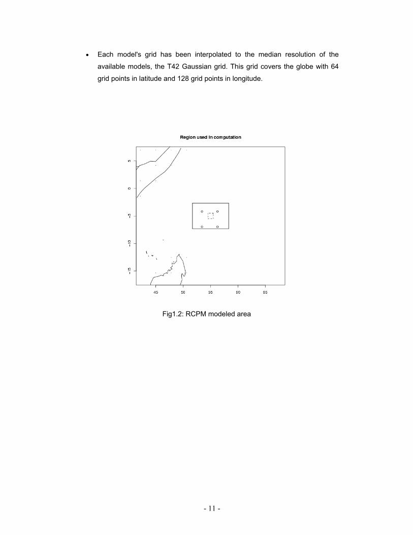
• Each model's grid has been interpolated to the median resolution of the
available models, the T42 Gaussian grid. This grid covers the globe with 64
grid points in latitude and 128 grid points in longitude.
Fig1.2: RCPM modeled area
- 12 -
Chapter 2
Global-Scale Climate Changes
2.0 Global-Scale Climate Changes The assessment of global-scale climate changes in this section of the V&A compares
two possible future climate change scenarios using the B2 mid-range emission with a
mid range climate sensitivity of 2.6 o C and the A1 high range emission with a high
range climate sensitivity of 4.6 o C. It is also valuable to consider more than one
emission scenarios and climate sensitivities in a V & A assessment, given the
uncertainty associated with future climate greenhouse gas and sulphur dioxide (SO2 )
emissions. Figures 2.1 to 2.6 are the MAGICC output comparisons between the
global carbon dioxide concentrations (ppmv), mean temperature (o C) and the mean
sea level changes (cm) derived from the two climate scenarios abbreviated as BM
and AH scenarios respectively.
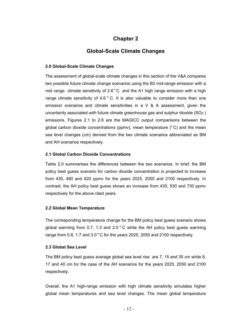
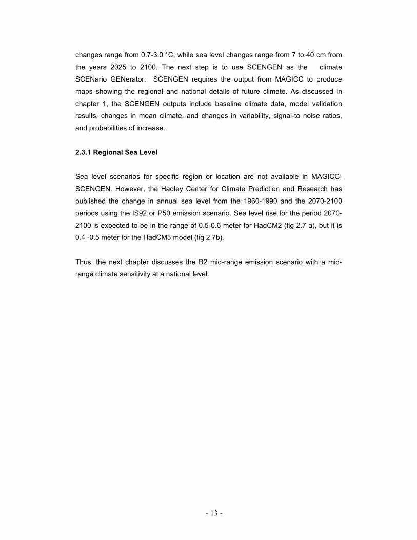
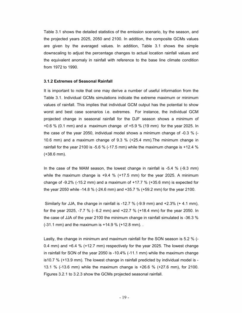
2.1 Global Carbon Dioxide Concentrations Table 2.0 summarises the differences between the two scenarios. In brief, the BM
policy best guess scenario for carbon dioxide concentration is projected to increase
from 430, 480 and 620 ppmv for the years 2025, 2050 and 2100 respectively. In
contrast, the AH policy best guess shows an increase from 430, 530 and 730 ppmv
respectively for the above cited years.
2.2 Global Mean Temperature The corresponding temperature change for the BM policy best guess scenario shows
global warming from 0.7, 1.3 and 2.5 o C while the AH policy best guess warming
range from 0.8, 1.7 and 3.0 o C for the years 2025, 2050 and 2100 respectively.
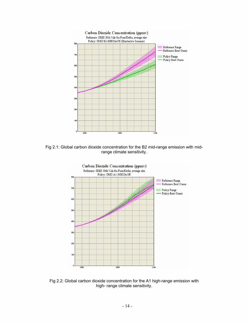
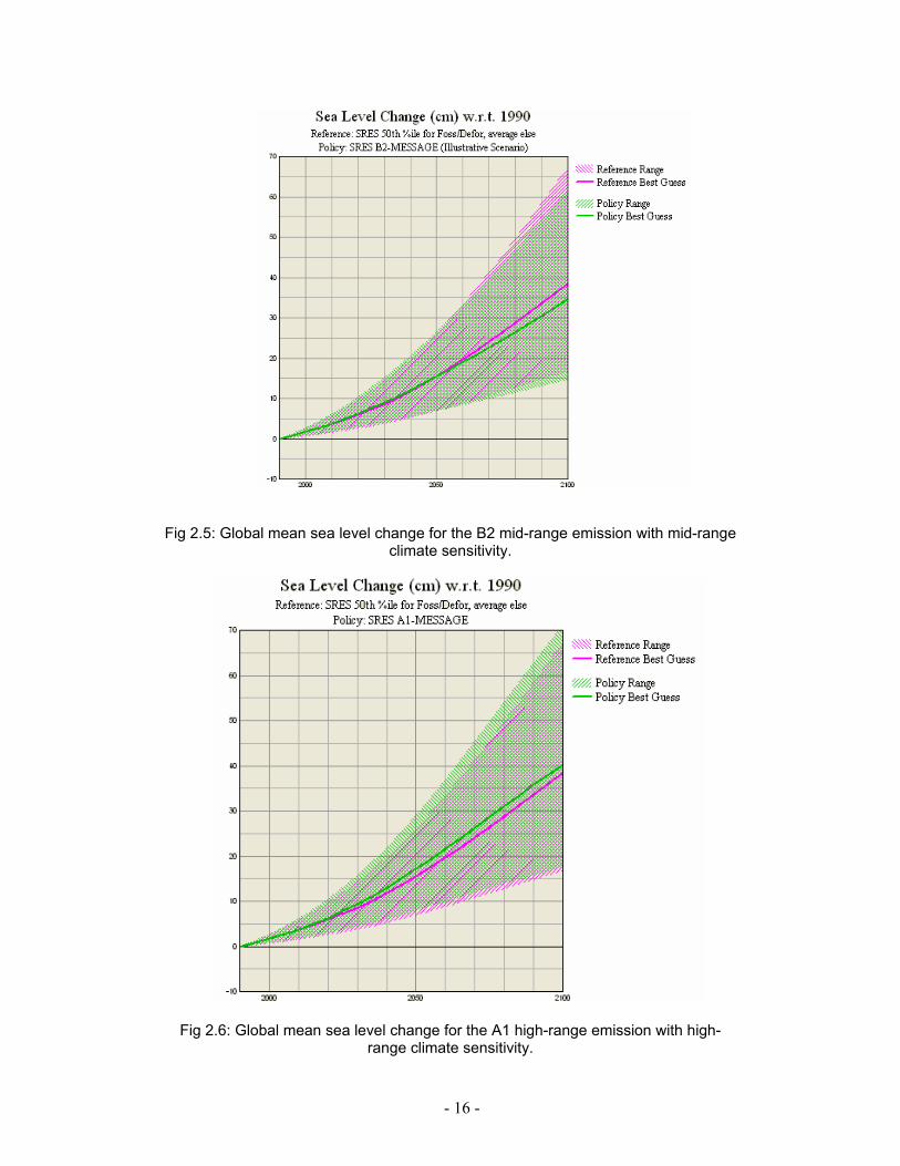
2.3 Global Sea Level The BM policy best guess average global sea level rise are 7, 15 and 35 cm while 8,
17 and 40 cm for the case of the AH scenarios for the years 2025, 2050 and 2100
respectively.
Overall, the A1 high-range emission with high climate sensitivity simulates higher
global mean temperatures and sea level changes. The mean global temperature
- 13 -
changes range from 0.7-3.0 o C, while sea level changes range from 7 to 40 cm from
the years 2025 to 2100. The next step is to use SCENGEN as the climate
SCENario GENerator. SCENGEN requires the output from MAGICC to produce
maps showing the regional and national details of future climate. As discussed in
chapter 1, the SCENGEN outputs include baseline climate data, model validation
results, changes in mean climate, and changes in variability, signal-to noise ratios,
and probabilities of increase.
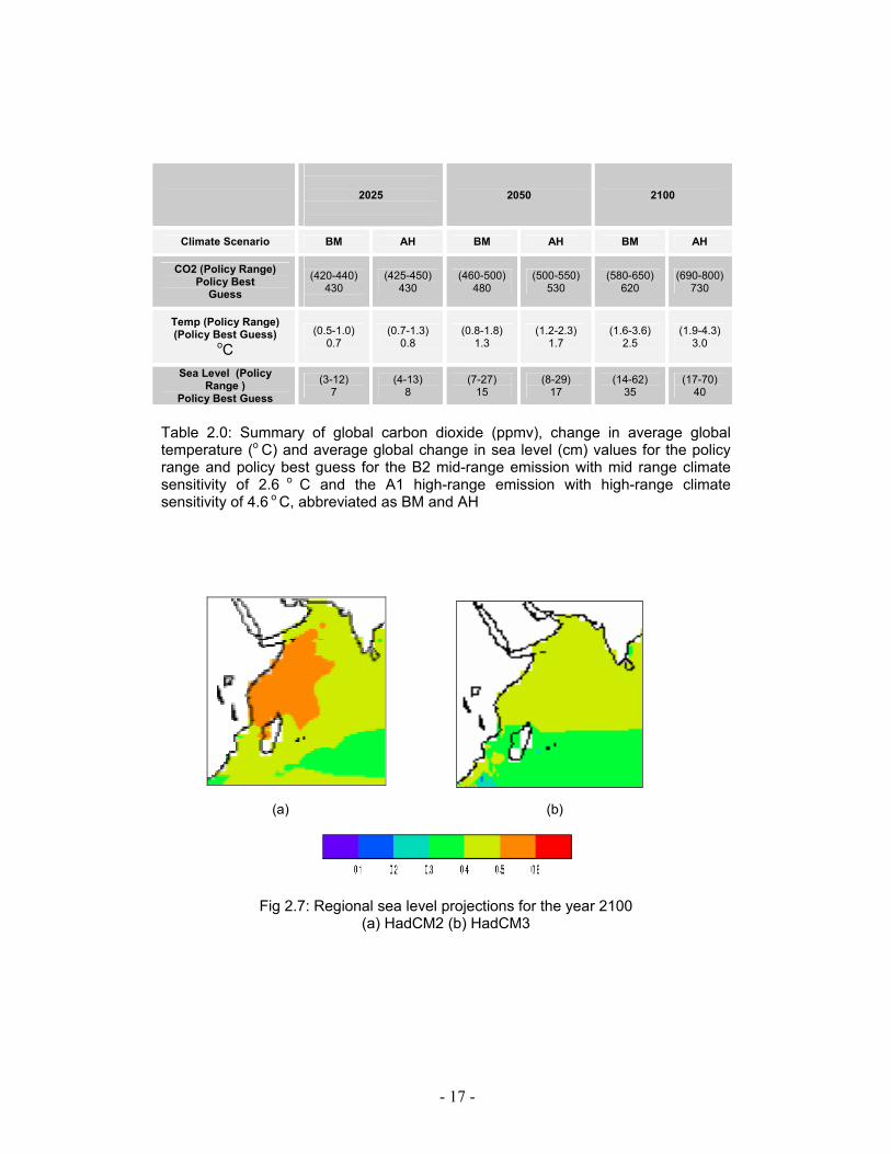
2.3.1 Regional Sea Level Sea level scenarios for specific region or location are not available in MAGICC-
SCENGEN. However, the Hadley Center for Climate Prediction and Research has
published the change in annual sea level from the 1960-1990 and the 2070-2100
periods using the IS92 or P50 emission scenario. Sea level rise for the period 2070-
2100 is expected to be in the range of 0.5-0.6 meter for HadCM2 (fig 2.7 a), but it is
0.4 -0.5 meter for the HadCM3 model (fig 2.7b).
Thus, the next chapter discusses the B2 mid-range emission scenario with a mid-
range climate sensitivity at a national level.
- 14 -
Fig 2.1: Global carbon dioxide concentration for the B2 mid-range emission with mid- range climate sensitivity.
Fig 2.2: Global carbon dioxide concentration for the A1 high-range emission with high- range climate sensitivity.

- 15 -
Fig 2.3: Global mean temperature change for the B2 mid-range emission with mid-
range climate sensitivity.
Fig 2.4: global mean temperature change for the A1 high- range emission with high- range climate sensitivity.
- 16 -
Fig 2.5: Global mean sea level change for the B2 mid-range emission with mid-range
climate sensitivity.
Fig 2.6: Global mean sea level change for the A1 high-range emission with high-range climate sensitivity.
- 17 -
2025
2050 2100
Climate Scenario BM AH BM AH BM AH
CO2 (Policy Range) Policy Best
Guess
(420-440)
430
(425-450) 430
(460-500) 480
(500-550) 530
(580-650) 620
(690-800) 730
Temp (Policy Range) (Policy Best Guess)
oC
(0.5-1.0) 0.7
(0.7-1.3) 0.8
(0.8-1.8) 1.3
(1.2-2.3) 1.7
(1.6-3.6) 2.5
(1.9-4.3) 3.0
Sea Level (Policy Range )
Policy Best Guess
(3-12) 7
(4-13) 8
(7-27) 15
(8-29) 17
(14-62) 35
(17-70) 40
Table 2.0: Summary of global carbon dioxide (ppmv), change in average global temperature (o C) and average global change in sea level (cm) values for the policy range and policy best guess for the B2 mid-range emission with mid range climate sensitivity of 2.6 o C and the A1 high-range emission with high-range climate sensitivity of 4.6 o C, abbreviated as BM and AH
(a) (b)
Fig 2.7: Regional sea level projections for the year 2100 (a) HadCM2 (b) HadCM3

- 18 -
Chapter 3
Climate Changes for B2 Mid-Range Emission with a Mid- Range Climate Sensitivity for the Mahe Area
3.0 Climate Changes for B2 Mid-Range Emission with a Mid -Range Climate Sensitivity for the Mahe Area This section analyses climate changes for the B2 mid-range emission with mid range
climate sensitivity at national level for the Mahe group using a simple downscaling
procedure. The analyses concentrate on examining individual GCMs output with the
objective of targeting climate extremes (i.e. maximum or lowest rainfall) which may
indicate critical thresholds for the quantification of risks and vulnerability. The
analyses provide a comprehensive assessment of model differences in simulating
spatial and temporal time scales. On the other hand, the composite analysis is simply
an average of the seven GCMs outputs. This technique is useful as it simplifies
analyses by generating a single climate pattern at a particular location.
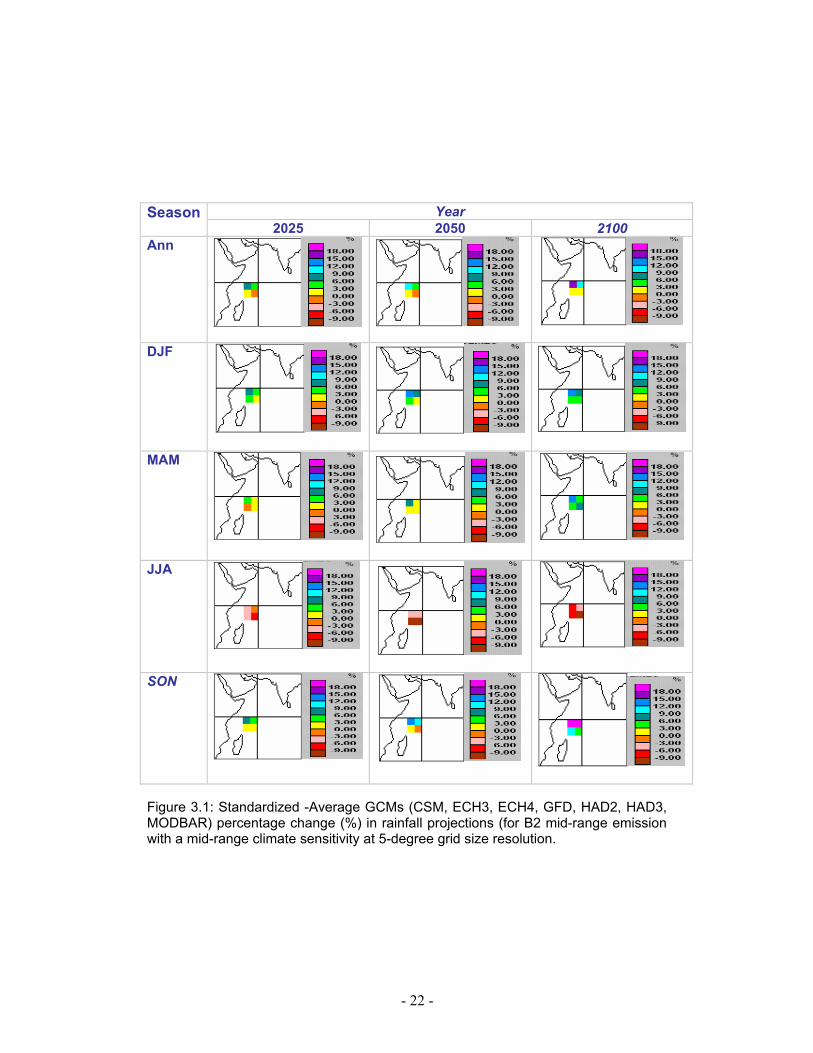
3.1.1 Spatial Rainfall Changes The Standardized-Average GCMs (CSM; ECH3, ECH4, GFD, HAD2, HAD3,
MODBAR) graphical spatial percentage change in rainfall projections for the B2 mid-
range emission with a mid-range climate sensitivity at a 5-degree grid size resolution
are shown in figure 3.1 for December, January, February (DJF), March, April, May
(MAM), June, July, August (JJA) and September, October, November (SON)
seasons of the projected years 2025, 2050 and 2100. It also includes the annual
percentage change (%) in precipitation. The scale indicates the average changes in
model precipitation for the area centered over Mahe and the inner islands. In
principle, one can apply the percentage change to any observed rainfall data set
located within this defined boundary. In summary, the spatial analysis shows positive
(wetter climate) changes for DJF, MAM and SON while negative (dryer climate) for
the JJA seasons respectively. In addition, the respective changes increase from the
years 2025 to 2100. However, the changes are not very clearly indicated due to the
variation of the pixels. This indeed reflects the normal characteristics of rainfall
spatial variability. Thus, further detailed analyses exploit the SCENGEN output files
which give full statistical details of the greenhouse-induced climatic values of the
defined area.
- 19 -
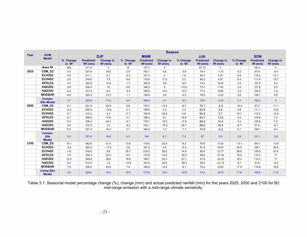
Table 3.1 shows the detailed statistics of the emission scenario, by the season, and
the projected years 2025, 2050 and 2100. In addition, the composite GCMs values
are given by the averaged values. In addition, Table 3.1 shows the simple
downscaling to adjust the percentage changes to actual location rainfall values and
the equivalent anomaly in rainfall with reference to the base line climate condition
from 1972 to 1990.
3.1.2 Extremes of Seasonal Rainfall It is important to note that one may derive a number of useful information from the
Table 3.1. Individual GCMs simulations indicate the extreme maximum or minimum
values of rainfall. This implies that individual GCM output has the potential to show
worst and best case scenarios i.e. extremes. For instance, the individual GCM
projected change in seasonal rainfall for the DJF season shows a minimum of
+0.6 % (0.1 mm) and a maximum change of +5.9 % (19 mm) for the year 2025. In
the case of the year 2050, individual model shows a minimum change of -0.3 % (-
10.6 mm) and a maximum change of 9.3 % (+25.4 mm).The minimum change in
rainfall for the year 2100 is -5.6 % (-17.5 mm) while the maximum change is +12.4 %
(+38.6 mm).
In the case of the MAM season, the lowest change in rainfall is -5.4 % (-9.3 mm)
while the maximum change is +9.4 % (+17.5 mm) for the year 2025. A minimum
change of -9.2% (-15.2 mm) and a maximum of +17.7 % (+35.6 mm) is expected for
the year 2050 while -14.8 % (-24.6 mm) and +35.7 % (+59.2 mm) for the year 2100.
Similarly for JJA, the change in rainfall is -12.7 % (-9.9 mm) and +2.3% (+ 4.1 mm),
for the year 2025, -7.7 % (- 6.2 mm) and +22.7 % (+18.4 mm) for the year 2050. In
the case of JJA of the year 2100 the minimum change in rainfall simulated is -36.3 %
(-31.1 mm) and the maximum is +14.9 % (+12.8 mm). .
Lastly, the change in minimum and maximum rainfall for the SON season is 5.2 % (-
0.4 mm) and +6.4 % (+12.7 mm) respectively for the year 2025. The lowest change
in rainfall for SON of the year 2050 is -10.4% (-11.1 mm) while the maximum change
is10.7 % (+13.9 mm). The lowest change in rainfall predicted by individual model is -
13.1 % (-13.6 mm) while the maximum change is +26.6 % (+27.6 mm), for 2100.
Figures 3.2.1 to 3.2.3 show the GCMs projected seasonal rainfall.
- 20 -
3.1.3 Composite of Seasonal Rainfall The composite model is simply an average of the individual GCMs to simplify and
generate a single regional climate pattern. The composite changes in rainfall for DJF,
MAM, JJA, and SON seasons for the year 2025 are +3.7 %, +2.0 %, -3.3% and
+3.8 % respectively (Table 3.1) The year 2050 composite changes in rainfall for the
same respective months are +5.3%, + 4.3%, +7.3 % and +2.4 %. The year 2100
composite rainfall changes are +4.9%, +10.5%, -10.8 %, and +11.8 % for the DJF,
MAM, JJA and SON seasons respectively.
Therefore, the largest increase in rainfall is expected during the DJF and SON
seasons, whereas JJA will have a negative change in the year 2025. It is surprising
to note that models are simulating a wetter climate during JJA season around the
2050s with a +7.3 % increase in rainfall. This is an important future climate change
pattern to be noted. Lastly, the composite values show a wetter-like season during
SON with an increase of +11.8 % in rainfall, while JJA becomes dryer with an
expected decrease in precipitation of -10.8 % for the year 2100. The composite
graph (Fig 3.2.4) shows clearly the rainfall trends as discussed earlier, i.e. wetter
rainy season and dryer dry season respectively for the years 2025 and 2100. In
contrast, rainfall projection for JJA of the year 2050 suggests relatively wetter dry
season.
The predicted composite rainfall anomaly for DJF when compared to the 1972-1990
periods mean of 311 mm is +11.6, +16.6, +15.4 mm respectively for the years 2025,
2050 and 2100. The rainfall anomalies for the MAM season compared to the base
line mean of 157.9 mm are +2.5, +6.1, +15.1 mm respectively. Similarly, the rainfall
anomaly with reference to the baseline mean of 81.1 mm for JJA is -4.2, +5.9, and -
8.7 mm respectively for the years 2025, 2050 and 2100. The SON rainfall anomalies
with reference to the 1972-1990 periods of 98.3 mm are +2.0, +2.7 and +11.6 mm
respectively.
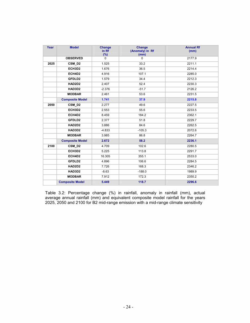
3.1.4 Extremes of Annual Rainfall The extreme annual change in precipitation is predicted by the ECH4 and HAD
GCMs (Table 3.2). For instance, the ECH4 GCM simulates maximum annual rainfall
changes of +4.9 %, +8.5 %, +16.3 % while the Had3 GCM simulates lowest rainfall
changes of - 2.4 %, -4.8 % and -8.6 % for the years 2025, 2050 and 2100
respectively.
- 21 -
Thus, the annual maximum rainfall is predicted to range between +107 and +355 mm
while the lowest model predicted rainfall ranges between -51.7 and -187 mm
annually.
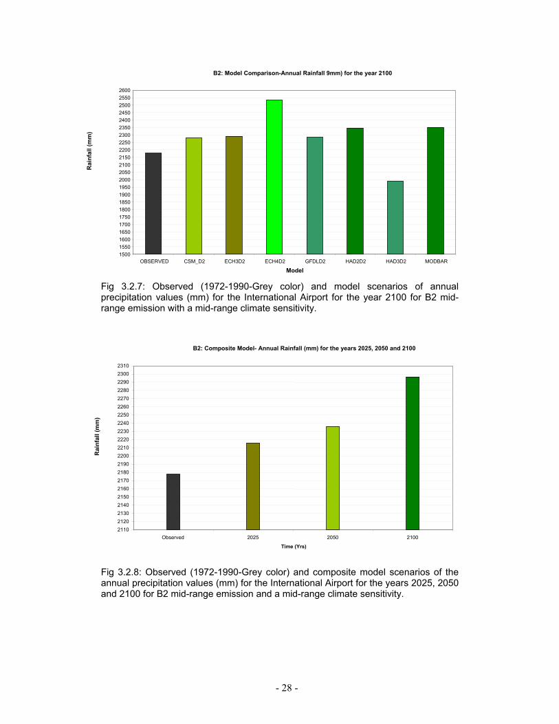
3.1.5 Composite of Annual Rainfall Table 3.2 also shows GCMs composites of annual rainfall. For example, the average
percentage change in average annual rainfall are +1.7 %, +2.7 %, and 5.5 % for the
years 2025, 2050 and 2100 respectively. Figure 3.2.8 shows the composite GCM
scenario of the annual precipitation values for the Mahe, Seychelles International
Airport for the years 2025, 2050 and 2100. The projected increases in annual rainfall
relative to the 1972-1990 periods mean of 2177.9 mm are +37.9, +58.2, and +118.7
mm for the years 2025, 2050 and 2100 respectively. Thus, rainfall is projected to
increase to a total of 2215.8, 2236.1 and 2296.6 mm annually by 2025, 2050 and
2100 correspondingly.
- 22 -
Year Season 2025 2050 2100
Ann
DJF
MAM
JJA
SON
Figure 3.1: Standardized -Average GCMs (CSM, ECH3, ECH4, GFD, HAD2, HAD3, MODBAR) percentage change (%) in rainfall projections (for B2 mid-range emission with a mid-range climate sensitivity at 5-degree grid size resolution.
- 23 -
Table 3.1: Seasonal model percentage change (%), change (mm) and actual predicted rainfall (mm) for the years 2025, 2050 and 2100 for B2
mid-range emission with a mid-range climate sensitivity.
Season DJF MAM JJA SON
Year
GCM
Model % Change
in Rf Predicted Rf (mm)
Change in Rf (mm)
% Change in Rf
Predicted Rf (mm)
Change in Rf (mm)
% Change in Rf
Predicted Rf (mm)
Change in Rf (mm)
% Change in Rf
Predicted Rf (mm)
Change in Rf (mm)
Base Rf 0.0 311.0 0 0 157.3 0 81.13 0 98.3 0 2025 CSM_D2 5.3 327.6 16.6 2.9 163.1 5.8 -3.9 79.4 -1.73 -5.2 97.9 -0.4
ECH3D2 0.6 311.1 0.1 -0.3 157.3 0 1.5 84.5 3.37 5.9 110.4 12.1 ECH4D2 2.8 318.9 7.9 9.4 174.8 17.5 2.3 85.2 4.07 6.4 111.0 12.7 GFDLD2 4.5 324.8 13.8 1.7 160.9 3.6 -9.5 74.2 -6.93 3.4 107.6 9.3 HAD2D2 5.9 330.0 19 4.6 166.3 9 -10.0 73.7 -7.43 3.4 107.6 9.3 HAD3D2 2.4 317.4 6.4 -5.4 148.0 -9.3 -12.7 71.2 -9.93 -3.2 100.2 1.9 MODBAR 4.6 325.3 14.3 1.1 159.9 2.6 -4.5 78.9 -2.23 3.8 108.1 9.8 Compo-
Site Model 3.7 322.6 11.6 2.0 160.4 3.1 -5.3 76.9 -4.23 2.1 100.3 2
2050 CSM_D2 8.1 331.9 20.9 5.9 170.7 13.4 -6.7 75.7 -5.4 -10.4 87.2 -11.1 ECH3D2 -0.3 300.4 -10.6 0.1 159.6 2.3 3.3 83.8 2.6 9.8 111.1 12.8 ECH4D2 3.7 315.3 4.3 17.7 192.9 35.6 4.6 84.8 3.7 10.7 112.2 13.9 GFDLD2 6.7 326.6 15.6 3.7 166.4 9.1 16.8 94.7 13.6 5.3 105.8 7.5 HAD2D2 9.3 336.4 25.4 9.1 176.7 19.4 17.8 95.6 14.4 5.3 105.8 7.5 HAD3D2 2.9 312.5 1.5 -9.2 142.1 -15.2 22.7 99.6 18.4 -6.7 91.6 -6.7 MODBAR 6.9 327.4 16.4 2.7 164.6 7.3 -7.7 74.9 -6.2 6.1 106.7 8.4 Compo-
Site Model
5.3 327.6 16.6 4.3 164 6.7 7.3 87 5.9 2.9 101.1 2.8
2100 CSM_D2 10.1 342.5 31.5 13.6 179.8 22.5 -6.2 75.8 -5.33 -13.1 84.7 -13.6 ECH3D2 -5.6 293.5 -17.5 2.6 161.5 4.2 12.4 91.8 10.67 24.9 124.1 25.8 ECH4D2 1.8 316.6 5.6 35.7 216.5 59.2 14.9 93.9 12.77 26.6 125.9 27.6 GFDLD2 7.5 334.3 23.3 9.4 172.8 15.5 -25.2 59.6 -21.53 16.4 115.3 17 HAD2D2 12.4 349.6 38.6 19.6 189.7 32.4 -27.1 57.9 -23.23 16.4 115.3 17 HAD3D2 0.4 312.4 1.4 -14.8 181.9 24.6 -36.3 50.0 -31.13 -6.1 91.9 -6.4 MODBAR 7.9 335.6 24.6 7.6 169.9 12.6 -8.1 74.2 -6.93 17.9 116.8 18.5 Comp-Site
Model 4.9 326.4 15.4 10.5 173.8 16.5 -10.8 72.4 -8.73 11.8 109.9 11.6
- 24 -
Table 3.2: Percentage change (%) in rainfall, anomaly in rainfall (mm), actual average annual rainfall (mm) and equivalent composite model rainfall for the years 2025, 2050 and 2100 for B2 mid-range emission with a mid-range climate sensitivity
Year Model Change in Rf (%)
Change (Anomaly) in Rf
(mm)
Annual Rf (mm)
OBSERVED 0 0 2177.9
2025 CSM_D2 1.525 33.2 2211.1 ECH3D2 1.676 36.5 2214.4 ECH4D2 4.916 107.1 2285.0 GFDLD2 1.579 34.4 2212.3 HAD2D2 2.407 52.4 2230.3 HAD3D2 -2.376 -51.7 2126.2 MODBAR 2.461 53.6 2231.5
Composite Model 1.741 37.9 2215.8
2050 CSM_D2 2.277 49.6 2227.5 ECH3D2 2.553 55.6 2233.5 ECH4D2 8.459 184.2 2362.1 GFDLD2 2.377 51.8 2229.7 HAD2D2 3.886 84.6 2262.5 HAD3D2 -4.833 -105.3 2072.6 MODBAR 3.985 86.8 2264.7
Composite Model 2.672 58.2 2236.1
2100 CSM_D2 4.709 102.6 2280.5 ECH3D2 5.225 113.8 2291.7 ECH4D2 16.305 355.1 2533.0 GFDLD2 4.896 106.6 2284.5 HAD2D2 7.726 168.3 2346.2 HAD3D2 -8.63 -188.0 1989.9 MODBAR 7.912 172.3 2350.2
Composite Model 5.449 118.7 2296.6

- 25 -
Fig 3.2.1: Observed (1972-1990 –Grey color) and scenarios of seasonal precipitation values (mm) for the International Airport, for B2 mid-range emissions with a mid-range climate sensitivity for the year 2025
Fig 3.2.2: Observed (1972-1990 –Grey color) and scenarios of seasonal precipitation values (mm) for the International Airport, for B2 mid-range emission with a mid-range climate sensitivity for the year 2025
B2: Seasonal Rainfall (mm) for the year 2025
0 20 40 60 80
100 120 140 160 180 200 220 240 260 280 300 320 340 360
DJF Airport Rf MAM Airport Rf JJA Airport Rf SON Airport Rf
Season (Months)
OBSERVED
CSM_D2ECH3D2
ECH4D2GFDLD2
HAD2D2
HAD3D2
MODBAR
B2: Seasonal Rainfall (mm) for the year 2050
0 20 40 60 80
100 120 140 160 180 200 220 240 260 280 300 320 340 360
DJF Airport Rf MAM Airport Rf JJA Airport Rf SON Airport Rf Season (months)
OBSERVED
CSM_D2
ECH3D2
ECH4D2
GFDLD2
HAD2D2
HAD3D2
MODBAR
Rai
nfal
l (m
m)
Rai
nfal
l (m
m)

- 26 -
Fig 3.2.3: Observed (1972-1990-Grey color) and scenarios of seasonal precipitation values (mm) for the International Airport for B2 mid-range emission with a mid-range climate sensitivity for the year 2100
Fig 3.2.4: Observed (1972-1990-Grey color) and composite model scenarios of seasonal precipitation values (mm) for the International Airport for the years 2025, 2050 and 2100 for B2 mid-range emission with a mid-range climate sensitivity.
B2: Seasonal Rainfall (mm) for the year 2100
0 20 40 60 80
100 120 140 160 180 200 220 240 260 280 300 320 340 360 380
DJF Airport Rf MAM Airport Rf JJA Airport Rf SON Airport Rf Season (Months)
OBSERVED
CSM_D2
ECH3D2
ECH4D2
GFDLD2
HAD2D2
HAD3D2
MODBAR
B2: Composite Model -Seasonal Rainfall (mm) for the years 2025, 2050 and 2100
50 60 70 80 90 100 110 120 130 140 150 160 170 180 190 200 210 220 230 240 250 260 270 280 290 300 310 320 330 340 350
DJF Airport Rf MAM Airport Rf JJA Airport Rf SON Airport Rf Season (Months)
Observed
2025
2050
2100
Rai
nfal
l (m
m)
Rai
nfal
l (m
m)
- 27 -
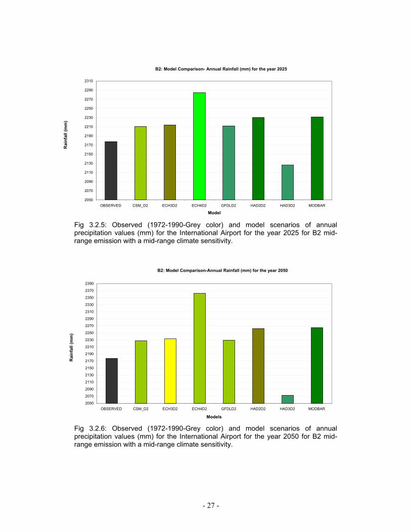
Fig 3.2.5: Observed (1972-1990-Grey color) and model scenarios of annual precipitation values (mm) for the International Airport for the year 2025 for B2 mid-range emission with a mid-range climate sensitivity.
Fig 3.2.6: Observed (1972-1990-Grey color) and model scenarios of annual precipitation values (mm) for the International Airport for the year 2050 for B2 mid-range emission with a mid-range climate sensitivity.
B2: Model Comparison- Annual Rainfall (mm) for the year 2025
2050 2070 2090 2110 2130 2150 2170 2190 2210 2230 2250 2270 2290 2310
OBSERVED CSM_D2 ECH3D2 ECH4D2 GFDLD2 HAD2D2 HAD3D2 MODBAR Model
B2: Model Comparison-Annual Rainfall (mm) for the year 2050
2050 2070 2090 2110 2130 2150 2170 2190 2210 2230 2250 2270 2290 2310 2330 2350 2370 2390
OBSERVED CSM_D2 ECH3D2 ECH4D2 GFDLD2 HAD2D2 HAD3D2 MODBAR Models
Rai
nfal
l (m
m)
Rai
nfal
l (m
m)
- 28 -
Fig 3.2.7: Observed (1972-1990-Grey color) and model scenarios of annual precipitation values (mm) for the International Airport for the year 2100 for B2 mid-range emission with a mid-range climate sensitivity.
Fig 3.2.8: Observed (1972-1990-Grey color) and composite model scenarios of the annual precipitation values (mm) for the International Airport for the years 2025, 2050 and 2100 for B2 mid-range emission and a mid-range climate sensitivity.
B2: Model Comparison-Annual Rainfall 9mm) for the year 2100
1500 1550 1600 1650 1700 1750 1800 1850 1900 1950 2000 2050 2100 2150 2200 2250 2300 2350 2400 2450 2500 2550 2600
OBSERVED CSM_D2 ECH3D2 ECH4D2 GFDLD2 HAD2D2 HAD3D2 MODBAR Model
B2: Composite Model- Annual Rainfall (mm) for the years 2025, 2050 and 2100
2110 2120 2130 2140 2150 2160 2170 2180 2190 2200 2210 2220 2230 2240 2250 2260 2270 2280 2290 2300 2310
Observed 2025 2050 2100 Time (Yrs)
Rai
nfal
l (m
m)
Rai
nfal
l (m
m)
- 29 -
B2: Composite GCMs and Location Rainfall for the years 2025, 2050 and 2100
16001700180019002000210022002300240025002600270028002900300031003200330034003500360037003800390040004100
Airp
ort
Raw
inds
onde
Sta
Le N
iol
Anse
La
Mou
che
Ans
e Fo
rban
Anse
Roy
al P
S
Bel
ombr
e
Bon
Esp
oir
Cas
cade
WW
Gra
nse
Anse
Res
earc
h
Her
mita
ge
La G
ogue
WW
La M
iser
e Fa
ir Vi
ew
New
Por
t
Qua
tre B
orne
Rec
eive
r
Roc
hon
WW
Satc
om
St L
ouis
TeaF
acto
ry
Pras
lin A
irStri
p
Locations
Rai
nfal
l (m
m)
Observed202520502100
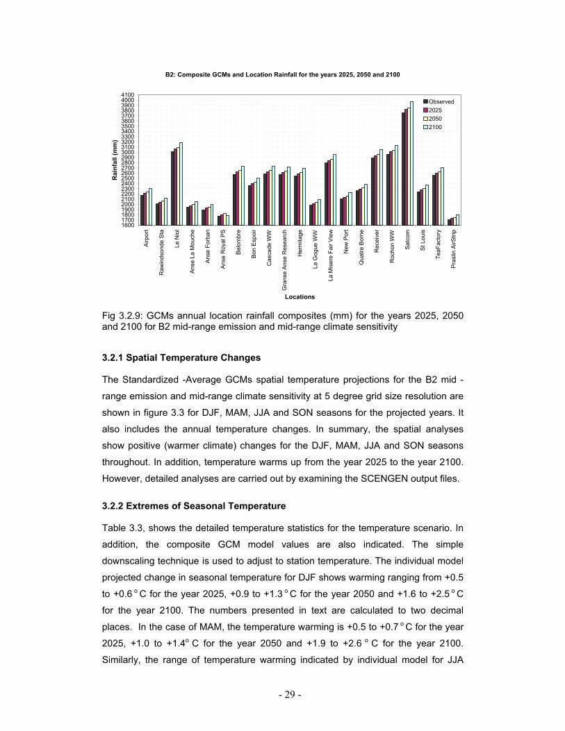
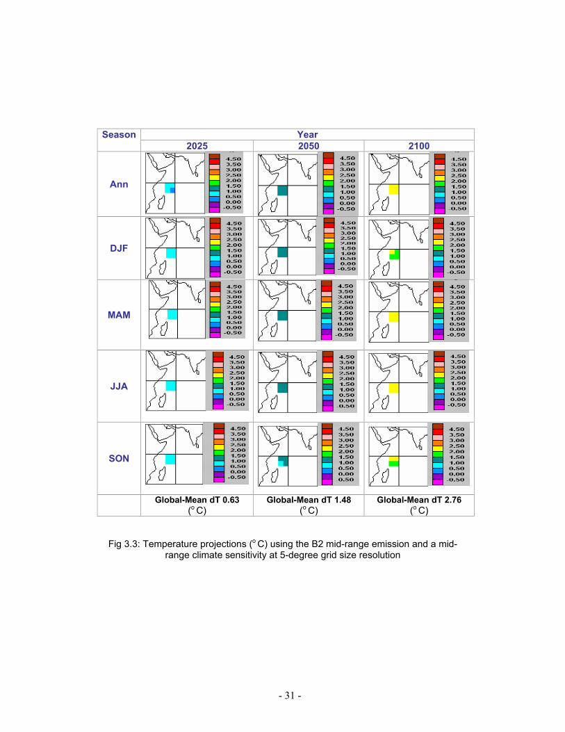
Fig 3.2.9: GCMs annual location rainfall composites (mm) for the years 2025, 2050 and 2100 for B2 mid-range emission and mid-range climate sensitivity 3.2.1 Spatial Temperature Changes The Standardized -Average GCMs spatial temperature projections for the B2 mid -
range emission and mid-range climate sensitivity at 5 degree grid size resolution are
shown in figure 3.3 for DJF, MAM, JJA and SON seasons for the projected years. It
also includes the annual temperature changes. In summary, the spatial analyses
show positive (warmer climate) changes for the DJF, MAM, JJA and SON seasons
throughout. In addition, temperature warms up from the year 2025 to the year 2100.
However, detailed analyses are carried out by examining the SCENGEN output files.
3.2.2 Extremes of Seasonal Temperature Table 3.3, shows the detailed temperature statistics for the temperature scenario. In
addition, the composite GCM model values are also indicated. The simple
downscaling technique is used to adjust to station temperature. The individual model
projected change in seasonal temperature for DJF shows warming ranging from +0.5
to +0.6 o C for the year 2025, +0.9 to +1.3 o C for the year 2050 and +1.6 to +2.5 o C
for the year 2100. The numbers presented in text are calculated to two decimal
places. In the case of MAM, the temperature warming is +0.5 to +0.7 o C for the year
2025, +1.0 to +1.4o C for the year 2050 and +1.9 to +2.6 o C for the year 2100.
Similarly, the range of temperature warming indicated by individual model for JJA
- 30 -
season ranges from +0.5 to +0.8 o C for the year 2025, +0.8 to +1.6 o C for the year
2050 and +1.6 to +2.9 o C for the year 2100. Lastly, the temperature warming for the
SON season ranges from +0.5 to +0.7 o C for the year 2025,+0.9 to +1.3 o C for 2050
and +1.6 to +2.5 o C for the year 2100. By considering only the upper range of the
individual model projected temperature change, it is observed that MAM, JJA will be
warmer by +2.6 and +2.9 o C by the year 2100. Figures 3.4.1 to 3.4.2 show the
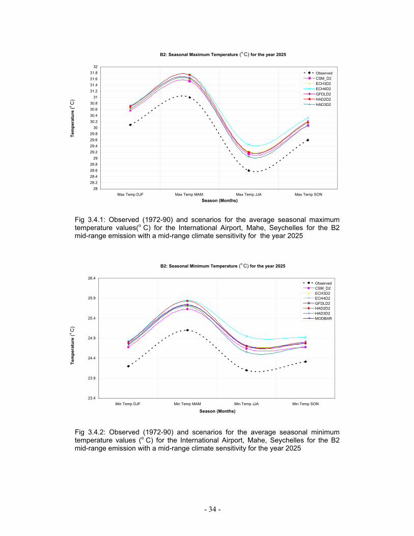
observed and the GCMs scenario average maximum and minimum temperature
values at the International Airport, Mahe, Seychelles.
3.2.3 Composite of Seasonal Temperature The DJF, MAM, JJA and SON seasonal GCMs composite of temperature changes
for the year 2025 range from +0.5 +0.6 o C. The warming in temperature for the year
2050 is +1.0, +1.2, +1.1 and +1.2 o C for the respective seasons, while the year 2100
temperature warming is +2.0, +2.2, +2.1, and +2.0 o C. The composite magnitude
shows increasing warming up to the year 2100, particularly during the MAM, JJA
seasons. This implies the projected future climate during the southeast monsoon will
be characterized by relatively warmer-like conditions. Figures 3.4.5 and 3.4.6 shows
observed and composite GCM scenarios of average maximum and minimum
temperature values for the years 2025, 2050 and 2100 at the International Airport,
Mahe, Seychelles.
3.2.4 Extreme of Annual Temperature The extreme annual percentage change in temperature is predicted by the ECH4
GCM. For instance ECH4 GCM projected warming in temperature is +0.7, +1.3, and
+2.6 o C for the years 2025, 2050 and 2100 respectively while the CSM GCM shows
lower warming of +0.5, +0.9 and +1.8 o C for the years 2025, 2050 and 2100
respectively (Table 3.3).
3.2.5 Composite of Annual Temperature The GCM composite shows warming of +0.6, +1.1 and +2.1 o C for the years 2025,
2050 and 2100 respectively. Thus, the annual mean temperature will gradually
become warmer by the year 2100 (table 3.4).
The next chapter analyses the second possible climate change scenario for the
Mahe area by considering the A1 high-range emission with high-range climate
sensitivity.
- 31 -
Year Season 2025 2050 2100
Ann
DJF
MAM
JJA
SON
Global-Mean dT 0.63
(o C) Global-Mean dT 1.48
(o C) Global-Mean dT 2.76
(o C)
Fig 3.3: Temperature projections (o C) using the B2 mid-range emission and a mid-range climate sensitivity at 5-degree grid size resolution
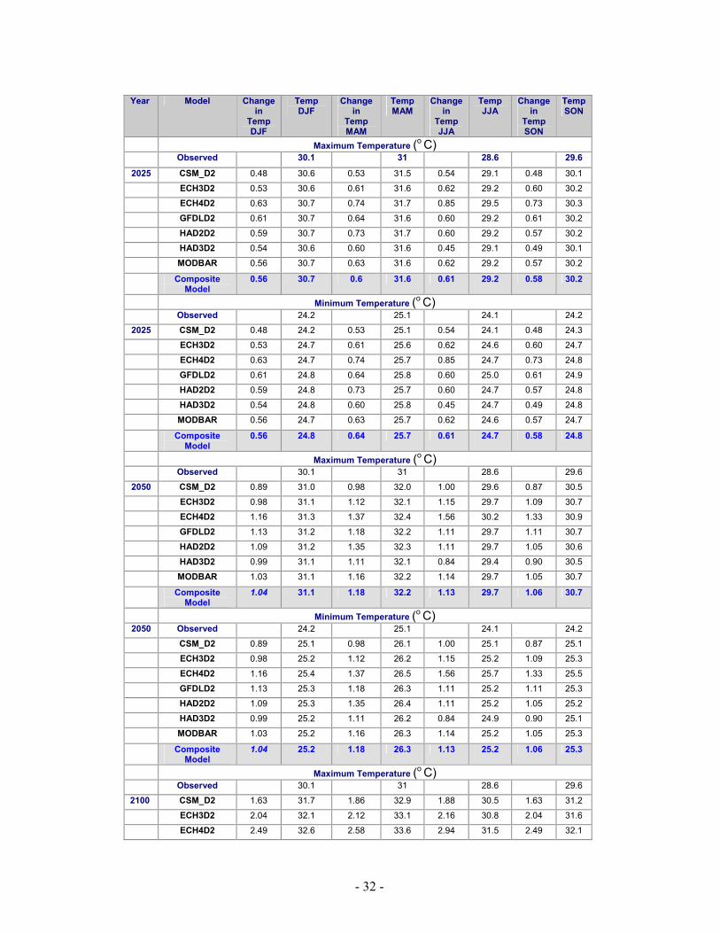
- 32 -
Year Model Change
in Temp DJF
Temp DJF
Change in
Temp MAM
Temp MAM
Change in
Temp JJA
Temp JJA
Change in
Temp SON
Temp SON
Maximum Temperature (o C) Observed 30.1 31 28.6 29.6
2025 CSM_D2 0.48 30.6 0.53 31.5 0.54 29.1 0.48 30.1
ECH3D2 0.53 30.6 0.61 31.6 0.62 29.2 0.60 30.2
ECH4D2 0.63 30.7 0.74 31.7 0.85 29.5 0.73 30.3
GFDLD2 0.61 30.7 0.64 31.6 0.60 29.2 0.61 30.2
HAD2D2 0.59 30.7 0.73 31.7 0.60 29.2 0.57 30.2
HAD3D2 0.54 30.6 0.60 31.6 0.45 29.1 0.49 30.1
MODBAR 0.56 30.7 0.63 31.6 0.62 29.2 0.57 30.2
Composite Model
0.56 30.7 0.6 31.6 0.61 29.2 0.58 30.2
Minimum Temperature (o C) Observed 24.2 25.1 24.1 24.2
2025 CSM_D2 0.48 24.2 0.53 25.1 0.54 24.1 0.48 24.3
ECH3D2 0.53 24.7 0.61 25.6 0.62 24.6 0.60 24.7
ECH4D2 0.63 24.7 0.74 25.7 0.85 24.7 0.73 24.8
GFDLD2 0.61 24.8 0.64 25.8 0.60 25.0 0.61 24.9
HAD2D2 0.59 24.8 0.73 25.7 0.60 24.7 0.57 24.8
HAD3D2 0.54 24.8 0.60 25.8 0.45 24.7 0.49 24.8
MODBAR 0.56 24.7 0.63 25.7 0.62 24.6 0.57 24.7
Composite Model
0.56 24.8 0.64 25.7 0.61 24.7 0.58 24.8
Maximum Temperature (o C) Observed 30.1 31 28.6 29.6
2050 CSM_D2 0.89 31.0 0.98 32.0 1.00 29.6 0.87 30.5
ECH3D2 0.98 31.1 1.12 32.1 1.15 29.7 1.09 30.7
ECH4D2 1.16 31.3 1.37 32.4 1.56 30.2 1.33 30.9
GFDLD2 1.13 31.2 1.18 32.2 1.11 29.7 1.11 30.7
HAD2D2 1.09 31.2 1.35 32.3 1.11 29.7 1.05 30.6
HAD3D2 0.99 31.1 1.11 32.1 0.84 29.4 0.90 30.5
MODBAR 1.03 31.1 1.16 32.2 1.14 29.7 1.05 30.7
Composite Model
1.04 31.1 1.18 32.2 1.13 29.7 1.06 30.7
Minimum Temperature (o C) 2050 Observed 24.2 25.1 24.1 24.2
CSM_D2 0.89 25.1 0.98 26.1 1.00 25.1 0.87 25.1
ECH3D2 0.98 25.2 1.12 26.2 1.15 25.2 1.09 25.3
ECH4D2 1.16 25.4 1.37 26.5 1.56 25.7 1.33 25.5
GFDLD2 1.13 25.3 1.18 26.3 1.11 25.2 1.11 25.3
HAD2D2 1.09 25.3 1.35 26.4 1.11 25.2 1.05 25.2
HAD3D2 0.99 25.2 1.11 26.2 0.84 24.9 0.90 25.1
MODBAR 1.03 25.2 1.16 26.3 1.14 25.2 1.05 25.3
Composite Model
1.04 25.2 1.18 26.3 1.13 25.2 1.06 25.3
Maximum Temperature (o C) Observed 30.1 31 28.6 29.6
2100 CSM_D2 1.63 31.7 1.86 32.9 1.88 30.5 1.63 31.2
ECH3D2 2.04 32.1 2.12 33.1 2.16 30.8 2.04 31.6
ECH4D2 2.49 32.6 2.58 33.6 2.94 31.5 2.49 32.1

- 33 -
GFDLD2 2.08 32.2 2.22 33.2 2.08 30.7 2.08 31.7
HAD2D2 1.96 32.1 2.55 33.5 2.10 30.7 1.96 31.6
HAD3D2 1.68 31.8 2.10 33.1 1.59 30.2 1.68 31.3
MODBAR 1.96 32.1 2.20 33.2 2.15 30.7 1.96 31.6
Composite Model
1.98 32.1 2.23 33.2 2.13 30.7 1.98 31.6
Minimum Temperature (o C)
Observed 24.2 25.1 24.1 24.2
2100 CSM_D2 1.63 25.8 1.86 27.0 1.88 26.0 1.63 25.8
ECH3D2 2.04 26.2 2.12 27.2 2.16 26.3 2.04 26.2
ECH4D2 2.49 26.7 2.58 27.7 2.94 27.0 2.49 26.7
GFDLD2 2.08 26.3 2.22 27.3 2.08 26.2 2.08 26.3
HAD2D2 1.96 26.2 2.55 27.6 2.10 26.2 1.96 26.2
HAD3D2 1.68 25.9 2.10 27.2 1.59 25.7 1.68 25.9
MODBAR 1.96 26.2 2.20 27.3 2.15 26.2 1.96 26.2
Composite Model
1.98 26.2 2.23 27.3 2.13 26.2 1.98 26.2
Table 3.3: (a) Observed, (b) change in temperature and (c) seasonal GCMs composite of temperature (o C) for the years 2025, 2050 and 2100 for B2 mid range emission with a mid-range climate sensitivity
Model Change in Temp 2025
(o C) Change in Temp 2050
(o C) Change in Temp 2100
(o C) CSM_D2 0.51 0.94 1.77
ECH3D2 0.59 1.09 2.05
ECH4D2 0.73 1.35 2.54
GFDLD2 0.61 1.13 2.13
HAD2D2 0.63 1.15 2.17
HAD3D2 0.52 0.95 1.80
MODBAR 0.59 1.09 2.07
Composite 0.60 1.10 2.07
Table 3.4: Annual GCMs temperature (o C) composites for the years 2025, 2050 and
2100 for B2 mid-range emission with a mid-range climate sensitivity
- 34 -
Fig 3.4.1: Observed (1972-90) and scenarios for the average seasonal maximum temperature values(o C) for the International Airport, Mahe, Seychelles for the B2 mid-range emission with a mid-range climate sensitivity for the year 2025
Fig 3.4.2: Observed (1972-90) and scenarios for the average seasonal minimum temperature values (o C) for the International Airport, Mahe, Seychelles for the B2 mid-range emission with a mid-range climate sensitivity for the year 2025
B2: Seasonal Maximum Temperature (o C) for the year 2025
28 28.2 28.4 28.6 28.8
29 29.2 29.4 29.6 29.8
30 30.2 30.4 30.6 30.8
31 31.2 31.4 31.6 31.8
32
Max Temp DJF Max Temp MAM Max Temp JJA Max Temp SON Season (Months)
Observed CSM_D2 ECH3D2 ECH4D2 GFDLD2 HAD2D2 HAD3D2
B2: Seasonal Minimum Temperature (o C) for the year 2025
23.4
23.9
24.4
24.9
25.4
25.9
26.4
Min Temp DJF Min Temp MAM Min Temp JJA Min Temp SON Season (Months)
Observed CSM_D2 ECH3D2 ECH4D2 GFDLD2 HAD2D2 HAD3D2 MODBAR
Tem
pera
ture
(o C
) Te
mpe
ratu
re (o
C)
- 35 -
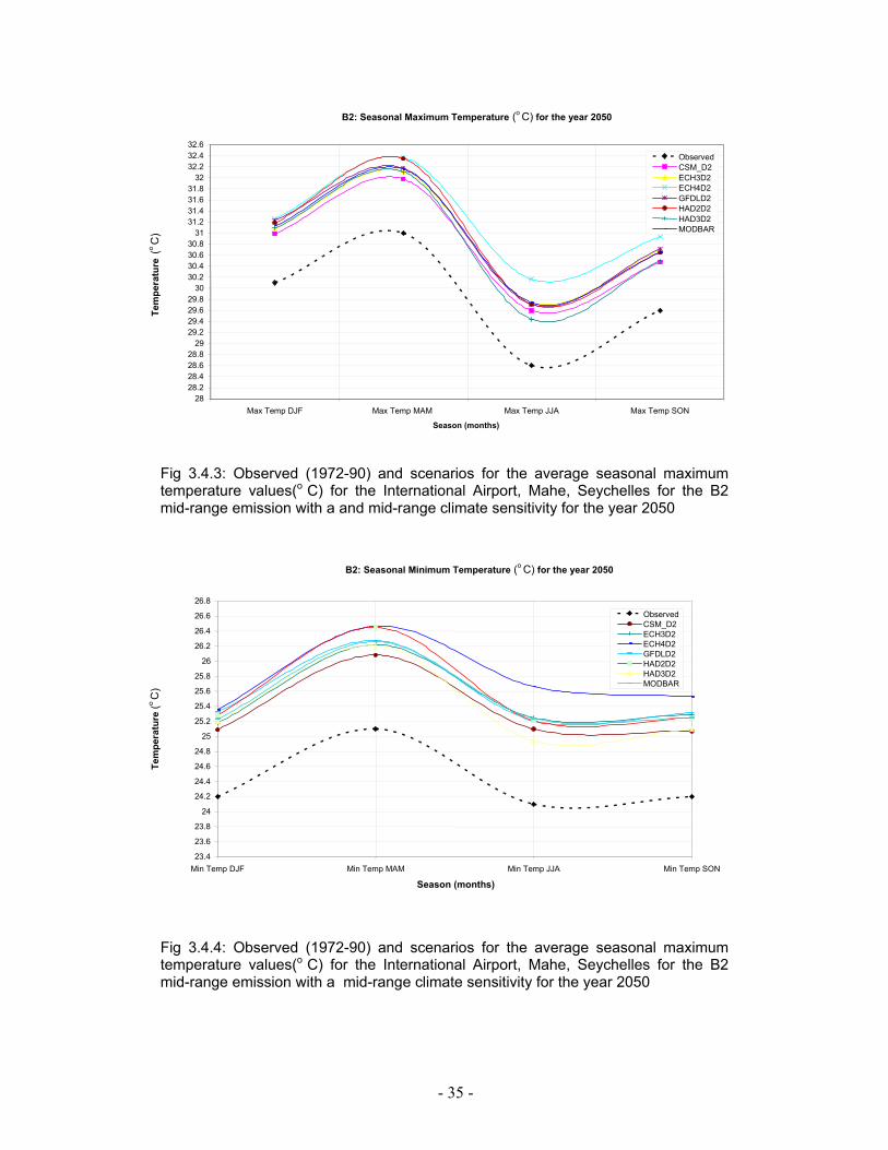
Fig 3.4.3: Observed (1972-90) and scenarios for the average seasonal maximum temperature values(o C) for the International Airport, Mahe, Seychelles for the B2 mid-range emission with a and mid-range climate sensitivity for the year 2050
Fig 3.4.4: Observed (1972-90) and scenarios for the average seasonal maximum temperature values(o C) for the International Airport, Mahe, Seychelles for the B2 mid-range emission with a mid-range climate sensitivity for the year 2050
B2: Seasonal Maximum Temperature (o C) for the year 2050
28 28.2 28.4 28.6 28.8
29 29.2 29.4 29.6 29.8
30 30.2 30.4 30.6 30.8
31 31.2 31.4 31.6 31.8
32 32.2 32.4 32.6
Max Temp DJF Max Temp MAM Max Temp JJA Max Temp SON Season (months)
ObservedCSM_D2 ECH3D2 ECH4D2 GFDLD2 HAD2D2 HAD3D2 MODBAR
B2: Seasonal Minimum Temperature (o C) for the year 2050
23.4 23.6 23.8
24 24.2 24.4 24.6 24.8
25 25.2 25.4 25.6 25.8
26 26.2 26.4 26.6 26.8
Min Temp DJF Min Temp MAM Min Temp JJA Min Temp SON
Season (months)
Observed CSM_D2 ECH3D2 ECH4D2 GFDLD2 HAD2D2 HAD3D2 MODBAR
Tem
pera
ture
(o C
) Te
mpe
ratu
re (o
C)
- 36 -
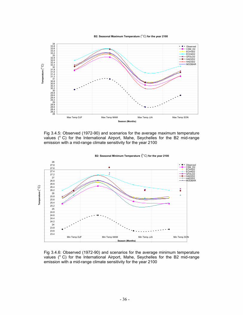
Fig 3.4.5: Observed (1972-90) and scenarios for the average maximum temperature values (o C) for the International Airport, Mahe, Seychelles for the B2 mid-range emission with a mid-range climate sensitivity for the year 2100
Fig 3.4.6: Observed (1972-90) and scenarios for the average minimum temperature values (o C) for the International Airport, Mahe, Seychelles for the B2 mid-range emission with a mid-range climate sensitivity for the year 2100
B2: Seasonal Maximum Temperature (o C) for the year 2100
28 28.2 28.4 28.6 28.8 29 29.2 29.4 29.6 29.8 30 30.2 30.4 30.6 30.8 31 31.2 31.4 31.6 31.8 32 32.2 32.4 32.6 32.8 33 33.2 33.4 33.6 33.8 34
Max Temp DJF Max Temp MAM Max Temp JJA Max Temp SON Season (Months)
ObservedCSM_D2 ECH3D2 ECH4D2 GFDLD2 HAD2D2 HAD3D2 MODBAR
B2: Seasonal Minimum Temperature (o C) for the year 2100
23.4 23.6 23.8
24 24.2 24.4 24.6 24.8
25 25.2 25.4 25.6 25.8
26 26.2 26.4 26.6 26.8
27 27.2 27.4 27.6 27.8
28
Min Temp DJF Min Temp MAM Min Temp JJA Min Temp SON Season (Months)
ObservedCSM_D2 ECH3D2 ECH4D2 GFDLD2 HAD2D2 HAD3D2 MODBAR
Tem
pera
ture
(o C
) Te
mpe
ratu
re (o
C)
- 37 -
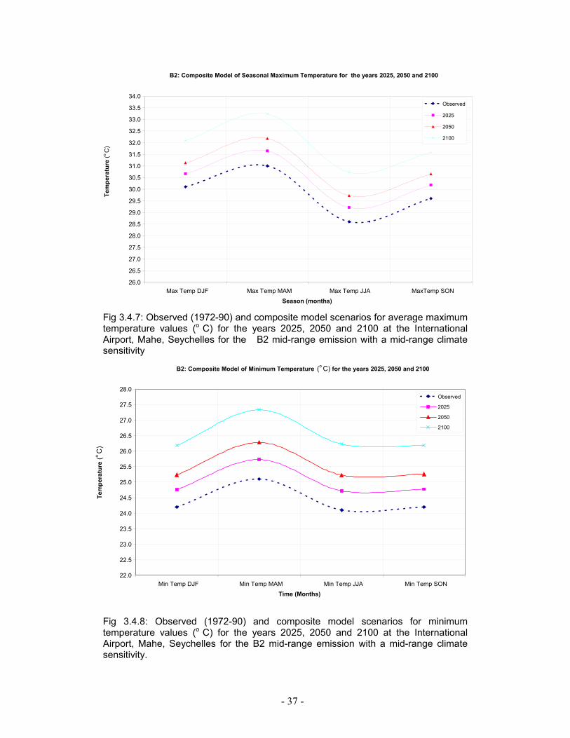
Fig 3.4.7: Observed (1972-90) and composite model scenarios for average maximum temperature values (o C) for the years 2025, 2050 and 2100 at the International Airport, Mahe, Seychelles for the B2 mid-range emission with a mid-range climate sensitivity
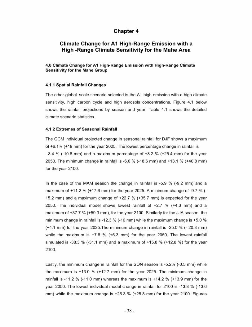
Fig 3.4.8: Observed (1972-90) and composite model scenarios for minimum temperature values (o C) for the years 2025, 2050 and 2100 at the International Airport, Mahe, Seychelles for the B2 mid-range emission with a mid-range climate sensitivity.
B2: Composite Model of Minimum Temperature (o C) for the years 2025, 2050 and 2100
22.0 22.5 23.0 23.5 24.0 24.5 25.0 25.5 26.0 26.5 27.0 27.5 28.0
Min Temp DJF Min Temp MAM Min Temp JJA Min Temp SON Time (Months)
Observed
2025 2050 2100
B2: Composite Model of Seasonal Maximum Temperature for the years 2025, 2050 and 2100
26.0 26.5 27.0 27.5 28.0 28.5 29.0 29.5 30.0 30.5 31.0 31.5 32.0 32.5 33.0 33.5 34.0
Max Temp DJF Max Temp MAM Max Temp JJA MaxTemp SON Season (months)
Tem
pera
ture
(o C
) Observed
2025 2050 2100
Tem
pera
ture
(o C
)
- 38 -
Chapter 4
Climate Change for A1 High-Range Emission with a High -Range Climate Sensitivity for the Mahe Area
4.0 Climate Change for A1 High-Range Emission with High-Range Climate Sensitivity for the Mahe Group 4.1.1 Spatial Rainfall Changes The other global–scale scenario selected is the A1 high emission with a high climate
sensitivity, high carbon cycle and high aerosols concentrations. Figure 4.1 below
shows the rainfall projections by season and year. Table 4.1 shows the detailed
climate scenario statistics.
4.1.2 Extremes of Seasonal Rainfall The GCM individual projected change in seasonal rainfall for DJF shows a maximum
of +6.1% (+19 mm) for the year 2025. The lowest percentage change in rainfall is
-3.4 % (-10.6 mm) and a maximum percentage of +8.2 % (+25.4 mm) for the year
2050. The minimum change in rainfall is -6.0 % (-18.6 mm) and +13.1 % (+40.8 mm)
for the year 2100.
In the case of the MAM season the change in rainfall is -5.9 % (-9.2 mm) and a
maximum of +11.2 % (+17.6 mm) for the year 2025. A minimum change of -9.7 % (-
15.2 mm) and a maximum change of +22.7 % (+35.7 mm) is expected for the year
2050. The individual model shows lowest rainfall of +2.7 % (+4.3 mm) and a
maximum of +37.7 % (+59.3 mm), for the year 2100. Similarly for the JJA season, the
minimum change in rainfall is -12.3 % (-10 mm) while the maximum change is +5.0 %
(+4.1 mm) for the year 2025.The minimum change in rainfall is -25.0 % (- 20.3 mm)
while the maximum is +7.8 % (+6.3 mm) for the year 2050. The lowest rainfall
simulated is -38.3 % (-31.1 mm) and a maximum of +15.8 % (+12.8 %) for the year
2100.
Lastly, the minimum change in rainfall for the SON season is -5.2% (-0.5 mm) while
the maximum is +13.0 % (+12.7 mm) for the year 2025. The minimum change in
rainfall is -11.2 % (-11.0 mm) whereas the maximum is +14.2 % (+13.9 mm) for the
year 2050. The lowest individual model change in rainfall for 2100 is -13.8 % (-13.6
mm) while the maximum change is +26.3 % (+25.8 mm) for the year 2100. Figures
- 39 -
4.2.1 to 4.2.3 show the GCMs projected seasonal rainfall for the years 2025, 2050
and 2100.
4.1.3 Composite of Seasonal Rainfall
The predicted composite anomaly in rainfall for the DJF season when compared to
the baseline mean of 311 mm is +11.2 mm, +10.5 mm and +16 mm respectively for
the years 2025, 2050 and 2100 (Table 4.1.1). Similarly, for the MAM season, the
predicted rainfall anomaly from the mean of 157.9 mm is +3.6, +9.7 and +23.8 mm.
The actual average rainfall anomaly for JJA season when compared to the current
mean of 81.1 mm is +3.0, -7.0 and -9.2 mm respectively for the years 2025, 2050
and 2100. The SON season projected rainfall anomaly from the mean of 98.3 mm is
+5.7, +4.6 and +12.2 mm respectively for the same target years. Figure 4.2.4 shows
the GCMs seasonal composite mean of precipitation for the Seychelles International
Airport.
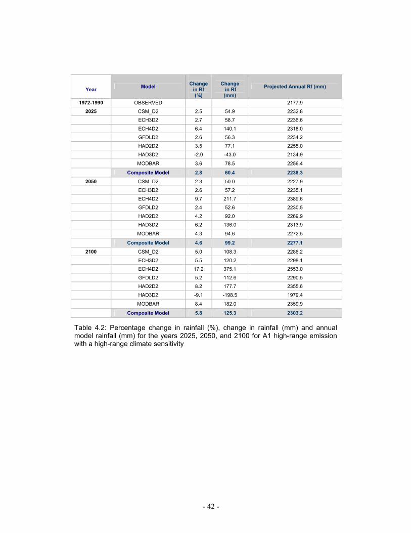
4.1.4 Extremes of Annual Rainfall The ECH4 model predicts the maximum annual change in rainfall of +6.4% (140 mm),
+9.7% (+211.7 mm), +17.2 % (+375mm) for the years 2025, 2050 and 2100
respectively while HAD3 model predicts the lowest change in rainfall of -2.0 % (-43
mm) for the year 2025 and -9.1% (-198 mm) for the year 2100 respectively (Table
4.1.2). However, the CSM model simulates the lowest change in rainfall of +2.3 %
(+50mm) for 2100. Figures 4.2.5 to 4.2.7 show individual GCMs maximum and
minimum annual changes in precipitation.
4.1.5 Composite of Annual Rainfall The GCMs composite of annual rainfall is +2.8 %, +4.6 %, and +5.8 % for the years
2025, 2050 and 2100 respectively (Table 4.1.2). Figure 4.2.8 shows the observed
(1972-1990-Grey color) and composite GCM model scenarios of the annual
precipitation values for the International Airport Mahe, Seychelles. The predicted
increase with reference to the 1972-1990 periods annual mean rainfall of 2177.9 mm
is +60.4, +99.2, and +125.3 mm for the years 2025, 2050 and 2100 respectively.

- 40 -
Season Year 2025 2050 2100 Ann
DJF
MAM
JJA
SON
Global-Mean dT 0.63(o C)
Global-Mean dT 1.48 (o C)
Global-Mean dT 2.76 (o C)
Fig 4.1: Standardized -Average GCMs (CSM, ECH3, ECH4, GFD, HAD2, HAD3, and MODBAR) rainfall projections for A1 high-range emission with high-range climate sensitivity at 5-degree grid size resolution.

- 41 -
Base Rf 311.0 157.3 81.13 98.3 2025 CSM_D2 5.3 327.6 16.6 3.7 163.1 5.9 -2.1 79.4 -1.7 -0.4 98.3 -0.4 ECH3D2 0.0 311.1 0.0 0.0 157.3 0.0 4.2 84.5 3.4 12.4 97.9 12.2 ECH4D2 2.5 318.9 7.9 11.2 174.8 17.6 5.0 85.2 4.1 13.0 110.4 12.7 GFDLD2 4.4 324.8 13.8 2.3 160.9 3.6 -8.5 74.2 -6.9 9.5 111.0 9.4 HAD2D2 6.1 330.0 19.0 5.7 166.3 9.0 -9.2 73.7 -7.4 9.5 107.6 9.4 HAD3D2 2.1 317.4 6.4 -5.9 148.0 -9.2 -12.3 71.2 -10.0 1.9 107.6 1.9 MODBAR 4.6 325.3 14.3 1.7 159.9 2.7 -2.8 78.9 -2.2 10.0 100.2 9.9 Composite
Model 3.6 322.2 11.1 2.7 161.5 4.2 -3.67 78.1 0.0 8.0 104.7 7.9
2050 CSM_D2 6.7 331.9 20.8 8.5 170.7 13.4 -5.7 76.5 -4.7 -11.2 87.2 -11.0 ECH3D2 -3.4 300.4 -10.6 1.5 159.6 2.3 6.2 86.2 5.0 13.1 111.1 12.9 ECH4D2 1.4 315.3 4.2 22.7 192.9 35.7 7.8 87.5 6.3 14.2 112.2 13.9 GFDLD2 5.0 326.6 15.6 5.8 166.4 9.1 -17.9 66.6 -14.5 7.7 105.8 7.5 HAD2D2 8.2 336.4 25.4 12.3 176.7 19.4 -19.1 65.6 -15.5 7.7 105.8 7.5 HAD3D2 0.5 312.5 1.5 -9.7 142.1 -15.2 -25.0 60.8 -20.3 -6.8 91.6 -6.6 MODBAR 5.3 327.4 16.4 4.7 164.6 7.4 -7.0 75.5 -5.6 8.6 106.7 8.5 Composite
Model 3.4 321.5 10.5 6.6 167.6 10.3 -8.7 74.1 0.0 4.8 102.9 4.7
2100 CSM_D2 10.7 344.3 33.3 14.4 179.8 22.6 -6.6 75.8 -5.3 -13.8 84.7 -13.6 ECH3D2 -6.0 292.5 -18.6 2.7 161.5 4.3 13.1 91.8 10.7 26.3 124.1 25.8 ECH4D2 1.9 317.0 5.9 37.7 216.5 59.3 15.8 93.9 12.8 28.1 125.9 27.6 GFDLD2 7.9 335.6 24.6 9.9 172.8 15.5 -26.6 59.6 -21.6 17.3 115.3 17.0 HAD2D2 13.1 351.8 40.8 20.7 189.7 32.5 -28.6 57.9 -23.2 17.3 115.3 17.0 HAD3D2 0.5 312.5 1.4 15.6 181.9 24.6 -38.3 50.0 -31.1 -6.5 91.9 -6.4 MODBAR 8.3 337.0 26.0 8.0 169.9 12.6 -8.6 74.2 -7.0 18.9 116.8 18.6 Composite
Model 5.2 327.2 16.2 15.6 181.7 24.5 -11.4 71.9 -9.2 12.5 110.5 12.3
Table 4.1.1: Observed, percentage change in rainfall (%), predicted seasonal rainfall (mm) and change in rainfall (mm) for the years 2025, 2050 and 2100 for A1 high-range emission with a high-range climate sensitivity
Season DJF MAM JJA SON
Year
GCM Model %
Change in Rf
Predicted Rf (mm)
Change in Rf (mm)
% Change in Rf
Predicted Rf (mm)
Change in Rf (mm)
% Change
in Rf
Predicted Rf (mm)
Change in Rf (mm)
% Change
in Rf
Predicted Rf (mm)
Change in Rf (mm)
- 42 -
Year Model
Change
in Rf (%)
Change
in Rf (mm)
Projected Annual Rf (mm)
1972-1990 OBSERVED 2177.9
2025 CSM_D2 2.5 54.9 2232.8
ECH3D2 2.7 58.7 2236.6
ECH4D2 6.4 140.1 2318.0
GFDLD2 2.6 56.3 2234.2
HAD2D2 3.5 77.1 2255.0
HAD3D2 -2.0 -43.0 2134.9
MODBAR 3.6 78.5 2256.4
Composite Model 2.8 60.4 2238.3
2050 CSM_D2 2.3 50.0 2227.9
ECH3D2 2.6 57.2 2235.1
ECH4D2 9.7 211.7 2389.6
GFDLD2 2.4 52.6 2230.5
HAD2D2 4.2 92.0 2269.9
HAD3D2 6.2 136.0 2313.9
MODBAR 4.3 94.6 2272.5
Composite Model 4.6 99.2 2277.1
2100 CSM_D2 5.0 108.3 2286.2
ECH3D2 5.5 120.2 2298.1
ECH4D2 17.2 375.1 2553.0
GFDLD2 5.2 112.6 2290.5
HAD2D2 8.2 177.7 2355.6
HAD3D2 -9.1 -198.5 1979.4
MODBAR 8.4 182.0 2359.9
Composite Model 5.8 125.3 2303.2 Table 4.2: Percentage change in rainfall (%), change in rainfall (mm) and annual model rainfall (mm) for the years 2025, 2050, and 2100 for A1 high-range emission with a high-range climate sensitivity
- 43 -
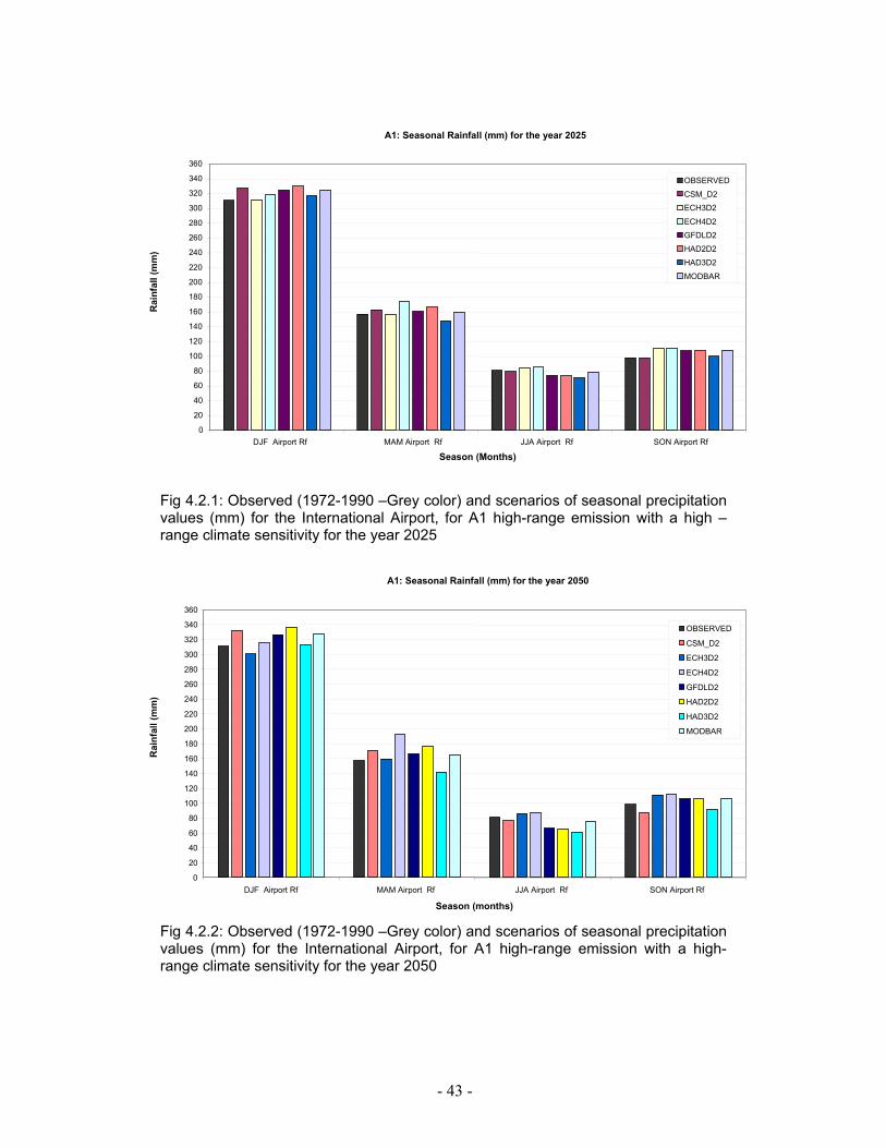
Fig 4.2.1: Observed (1972-1990 –Grey color) and scenarios of seasonal precipitation values (mm) for the International Airport, for A1 high-range emission with a high –range climate sensitivity for the year 2025
Fig 4.2.2: Observed (1972-1990 –Grey color) and scenarios of seasonal precipitation values (mm) for the International Airport, for A1 high-range emission with a high-range climate sensitivity for the year 2050
A1: Seasonal Rainfall (mm) for the year 2025
0 20 40 60 80
100 120 140 160 180 200 220 240 260 280 300 320 340 360
DJF Airport Rf MAM Airport Rf JJA Airport Rf SON Airport Rf Season (Months)
OBSERVED
CSM_D2ECH3D2
ECH4D2GFDLD2
HAD2D2
HAD3D2
MODBAR
A1: Seasonal Rainfall (mm) for the year 2050
0 20 40 60 80
100 120 140 160 180 200 220 240 260 280 300 320 340 360
DJF Airport Rf MAM Airport Rf JJA Airport Rf SON Airport Rf Season (months)
OBSERVED
CSM_D2
ECH3D2
ECH4D2
GFDLD2
HAD2D2
HAD3D2
MODBAR
Rai
nfal
l (m
m)
Rai
nfal
l (m
m)
- 44 -
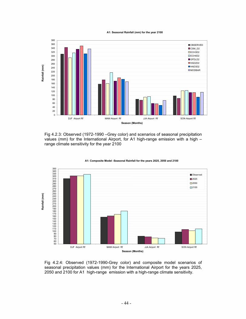
Fig 4.2.3: Observed (1972-1990 –Grey color) and scenarios of seasonal precipitation values (mm) for the International Airport, for A1 high-range emission with a high –range climate sensitivity for the year 2100
Fig 4.2.4: Observed (1972-1990-Grey color) and composite model scenarios of seasonal precipitation values (mm) for the International Airport for the years 2025, 2050 and 2100 for A1 high-range emission with a high-range climate sensitivity.
A1: Seasonal Rainfall (mm) for the year 2100
0 20 40 60 80
100 120 140 160 180 200 220 240 260 280 300 320 340 360 380
DJF Airport Rf MAM Airport Rf JJA Airport Rf SON Airport Rf Season (Months)
OBSERVEDCSM_D2ECH3D2ECH4D2GFDLD2HAD2D2HAD3D2MODBAR
A1: Composite Model -Seasonal Rainfall for the years 2025, 2050 and 2100
50 60 70 80 90 100 110 120 130 140 150 160 170 180 190 200 210 220 230 240 250 260 270 280 290 300 310 320 330 340 350
DJF Airport Rf MAM Airport Rf JJA Airport Rf SON Airport Rf Season (Months)
Observed
2025 2050 2100
Rai
nfal
l (m
m)
Rai
nfal
l (m
m)
- 45 -
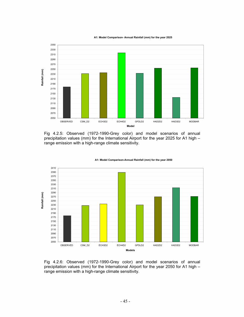
Fig 4.2.5: Observed (1972-1990-Grey color) and model scenarios of annual precipitation values (mm) for the International Airport for the year 2025 for A1 high –range emission with a high-range climate sensitivity.
Fig 4.2.6: Observed (1972-1990-Grey color) and model scenarios of annual precipitation values (mm) for the International Airport for the year 2050 for A1 high –range emission with a high-range climate sensitivity.
A1: Model Comparison- Annual Rainfall (mm) for the year 2025
2050 2070 2090 2110 2130 2150 2170 2190 2210 2230 2250 2270 2290 2310 2330 2350
OBSERVED CSM_D2 ECH3D2 ECH4D2 GFDLD2 HAD2D2 HAD3D2 MODBAR
Model
A1: Model Comparison-Annual Rainfall (mm) for the year 2050
2050 2070 2090 2110 2130 2150 2170 2190 2210 2230 2250 2270 2290 2310 2330 2350 2370 2390 2410
OBSERVED CSM_D2 ECH3D2 ECH4D2 GFDLD2 HAD2D2 HAD3D2 MODBAR
Models
Rai
nfal
l (m
m)
Rai
nfal
l (m
m)
- 46 -
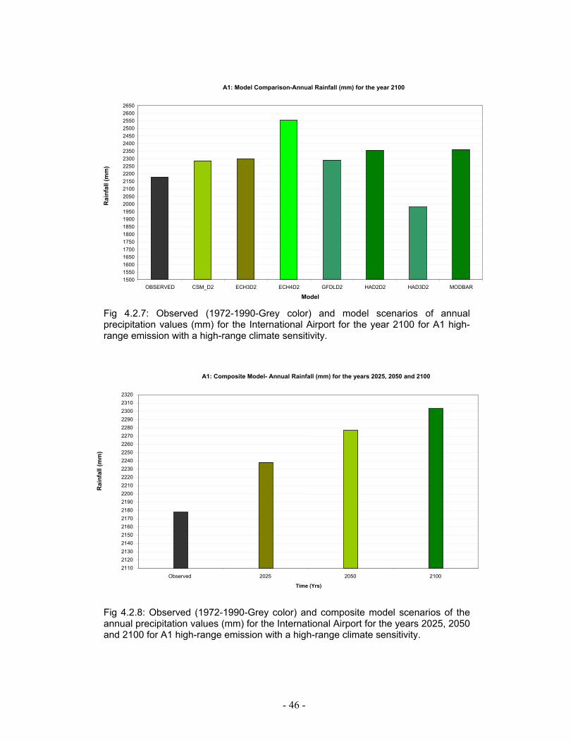
Fig 4.2.7: Observed (1972-1990-Grey color) and model scenarios of annual precipitation values (mm) for the International Airport for the year 2100 for A1 high-range emission with a high-range climate sensitivity.
Fig 4.2.8: Observed (1972-1990-Grey color) and composite model scenarios of the annual precipitation values (mm) for the International Airport for the years 2025, 2050 and 2100 for A1 high-range emission with a high-range climate sensitivity.
A1: Model Comparison-Annual Rainfall (mm) for the year 2100
1500 1550 1600 1650 1700 1750 1800 1850 1900 1950 2000 2050 2100 2150 2200 2250 2300 2350 2400 2450 2500 2550 2600 2650
OBSERVED CSM_D2 ECH3D2 ECH4D2 GFDLD2 HAD2D2 HAD3D2 MODBAR
Model
A1: Composite Model- Annual Rainfall (mm) for the years 2025, 2050 and 2100
2110 2120 2130 2140 2150 2160 2170 2180 2190 2200 2210 2220 2230 2240 2250 2260 2270 2280 2290 2300 2310 2320
Observed 2025 2050 2100 Time (Yrs)
Rai
nfal
l (m
m)
Rai
nfal
l (m
m)

- 47 -
A1: Composite Model -Location Rainfall (mm) for the years 2025, 2050 and 2100
1500165018001950210022502400255027002850300031503300345036003750390040504200
Airp
ort
Raw
inds
onde
Sta
Le N
iol
Anse
La
Mou
che
Ans
e Fo
rban
Anse
Roy
al P
S
Belo
mbr
e
Bon
Espo
ir
Cas
cade
WW
Gra
nse
Anse
Res
earc
h
Her
mita
ge
La G
ogue
WW
La M
iser
e Fa
ir Vi
ew
New
Por
t
Qua
tre B
orne
Rec
eive
r
Roc
hon
WW
Satc
om
St L
ouis
TeaF
acto
ry
Pra
slin
AirS
trip
Locations
Rai
nfal
l (m
m)
Observed202520502100
Fig 4.2.9: GCMs annual location rainfall (mm) composite for the years 2025, 2050 and 2100 for A1 high-range emission with high- range climate sensitivity
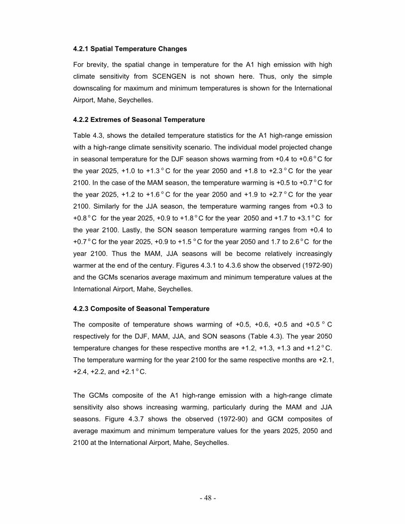
- 48 -
4.2.1 Spatial Temperature Changes For brevity, the spatial change in temperature for the A1 high emission with high
climate sensitivity from SCENGEN is not shown here. Thus, only the simple
downscaling for maximum and minimum temperatures is shown for the International
Airport, Mahe, Seychelles.
4.2.2 Extremes of Seasonal Temperature Table 4.3, shows the detailed temperature statistics for the A1 high-range emission
with a high-range climate sensitivity scenario. The individual model projected change
in seasonal temperature for the DJF season shows warming from +0.4 to +0.6 o C for
the year 2025, +1.0 to +1.3 o C for the year 2050 and +1.8 to +2.3 o C for the year
2100. In the case of the MAM season, the temperature warming is +0.5 to +0.7 o C for
the year 2025, +1.2 to +1.6 o C for the year 2050 and +1.9 to +2.7 o C for the year
2100. Similarly for the JJA season, the temperature warming ranges from +0.3 to
+0.8 o C for the year 2025, +0.9 to +1.8 o C for the year 2050 and +1.7 to +3.1 o C for
the year 2100. Lastly, the SON season temperature warming ranges from +0.4 to
+0.7 o C for the year 2025, +0.9 to +1.5 o C for the year 2050 and 1.7 to 2.6 o C for the
year 2100. Thus the MAM, JJA seasons will be become relatively increasingly
warmer at the end of the century. Figures 4.3.1 to 4.3.6 show the observed (1972-90)
and the GCMs scenarios average maximum and minimum temperature values at the
International Airport, Mahe, Seychelles.
4.2.3 Composite of Seasonal Temperature The composite of temperature shows warming of +0.5, +0.6, +0.5 and +0.5 o C
respectively for the DJF, MAM, JJA, and SON seasons (Table 4.3). The year 2050
temperature changes for these respective months are +1.2, +1.3, +1.3 and +1.2 o C.
The temperature warming for the year 2100 for the same respective months are +2.1,
+2.4, +2.2, and +2.1 o C.
The GCMs composite of the A1 high-range emission with a high-range climate
sensitivity also shows increasing warming, particularly during the MAM and JJA
seasons. Figure 4.3.7 shows the observed (1972-90) and GCM composites of
average maximum and minimum temperature values for the years 2025, 2050 and
2100 at the International Airport, Mahe, Seychelles.
- 49 -
4.2.4 Extreme of Annual Temperature The annual maximum change in temperature is predicted by the ECH4 model (Table
not shown). For instance ECH4 shows warming from +0.7, +1.3, and +2.7 o C for the
years 2025, 2050 and 2100 respectively while the CSM shows lower temperature
change of +0.6, +0.9 and +1.8 o C for the years 2025, 2050 and 2100 respectively.
4.2.5 Composite of Annual Temperature The composite of annual temperature shows warming of +0.5, +1.3 and +2.2 o C respectively. Thus, the annual mean temperature will become warmer by the year 2100.
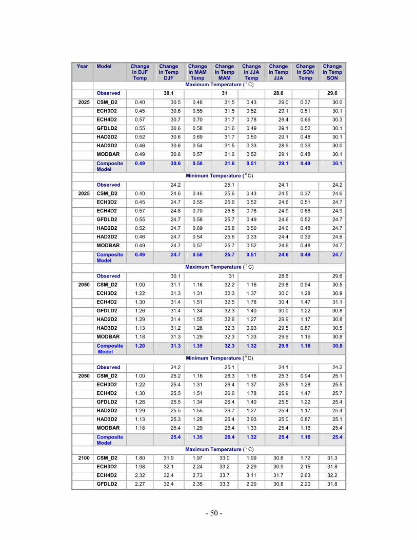
- 50 -
Year Model Change
in DJF Temp
Change in Temp
DJF
Change in MAM Temp
Change in Temp
MAM
Change in JJA Temp
Change in Temp
JJA
Change in SON Temp
Change in Temp
SON Maximum Temperature ( o C) Observed 30.1 31 28.6 29.6
2025 CSM_D2 0.40 30.5 0.46 31.5 0.43 29.0 0.37 30.0
ECH3D2 0.45 30.6 0.55 31.5 0.52 29.1 0.51 30.1
ECH4D2 0.57 30.7 0.70 31.7 0.78 29.4 0.66 30.3
GFDLD2 0.55 30.6 0.58 31.6 0.49 29.1 0.52 30.1
HAD2D2 0.52 30.6 0.69 31.7 0.50 29.1 0.48 30.1
HAD3D2 0.46 30.6 0.54 31.5 0.33 28.9 0.39 30.0
MODBAR 0.49 30.6 0.57 31.6 0.52 29.1 0.48 30.1
Composite Model
0.49 30.6 0.58 31.6 0.51 29.1 0.49 30.1
Minimum Temperature ( o C)
Observed 24.2 25.1 24.1 24.2
2025 CSM_D2 0.40 24.6 0.46 25.6 0.43 24.5 0.37 24.6
ECH3D2 0.45 24.7 0.55 25.6 0.52 24.6 0.51 24.7
ECH4D2 0.57 24.8 0.70 25.8 0.78 24.9 0.66 24.9
GFDLD2 0.55 24.7 0.58 25.7 0.49 24.6 0.52 24.7
HAD2D2 0.52 24.7 0.69 25.8 0.50 24.6 0.48 24.7
HAD3D2 0.46 24.7 0.54 25.6 0.33 24.4 0.39 24.6
MODBAR 0.49 24.7 0.57 25.7 0.52 24.6 0.48 24.7
Composite Model
0.49 24.7 0.58 25.7 0.51 24.6 0.49 24.7
Maximum Temperature ( o C)
Observed 30.1 31 28.6 29.6
2050 CSM_D2 1.00 31.1 1.16 32.2 1.16 29.8 0.94 30.5
ECH3D2 1.22 31.3 1.31 32.3 1.37 30.0 1.28 30.9
ECH4D2 1.30 31.4 1.51 32.5 1.78 30.4 1.47 31.1
GFDLD2 1.26 31.4 1.34 32.3 1.40 30.0 1.22 30.8
HAD2D2 1.29 31.4 1.55 32.6 1.27 29.9 1.17 30.8
HAD3D2 1.13 31.2 1.28 32.3 0.93 29.5 0.87 30.5
MODBAR 1.18 31.3 1.29 32.3 1.33 29.9 1.16 30.8
Composite Model
1.20 31.3 1.35 32.3 1.32 29.9 1.16 30.8
Minimum Temperature ( o C)
Observed 24.2 25.1 24.1 24.2
2050 CSM_D2 1.00 25.2 1.16 26.3 1.16 25.3 0.94 25.1
ECH3D2 1.22 25.4 1.31 26.4 1.37 25.5 1.28 25.5
ECH4D2 1.30 25.5 1.51 26.6 1.78 25.9 1.47 25.7
GFDLD2 1.26 25.5 1.34 26.4 1.40 25.5 1.22 25.4
HAD2D2 1.29 25.5 1.55 26.7 1.27 25.4 1.17 25.4
HAD3D2 1.13 25.3 1.28 26.4 0.93 25.0 0.87 25.1
MODBAR 1.18 25.4 1.29 26.4 1.33 25.4 1.16 25.4
Composite Model
25.4 1.35 26.4 1.32 25.4 1.16 25.4
Maximum Temperature ( o C) 2100 CSM_D2 1.80 31.9 1.97 33.0 1.99 30.6 1.72 31.3
ECH3D2 1.98 32.1 2.24 33.2 2.29 30.9 2.15 31.8
ECH4D2 2.32 32.4 2.73 33.7 3.11 31.7 2.63 32.2
GFDLD2 2.27 32.4 2.35 33.3 2.20 30.8 2.20 31.8
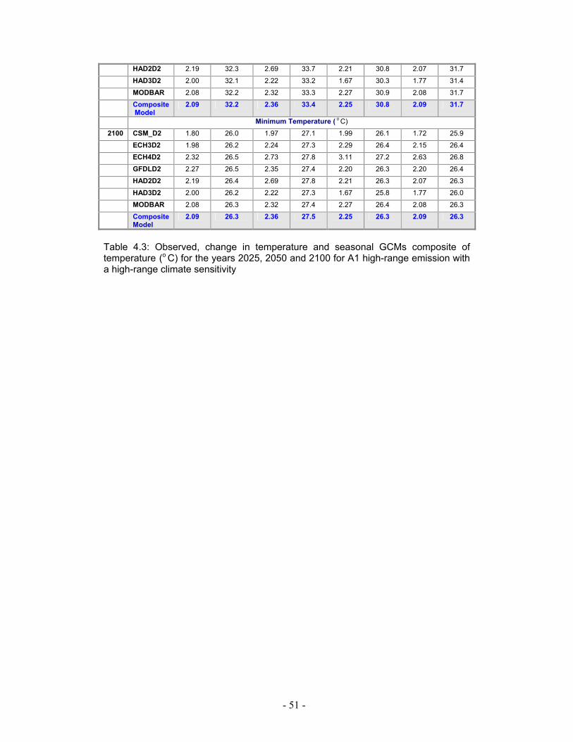
- 51 -
HAD2D2 2.19 32.3 2.69 33.7 2.21 30.8 2.07 31.7
HAD3D2 2.00 32.1 2.22 33.2 1.67 30.3 1.77 31.4
MODBAR 2.08 32.2 2.32 33.3 2.27 30.9 2.08 31.7
Composite Model
2.09 32.2 2.36 33.4 2.25 30.8 2.09 31.7
Minimum Temperature ( o C) 2100 CSM_D2 1.80 26.0 1.97 27.1 1.99 26.1 1.72 25.9
ECH3D2 1.98 26.2 2.24 27.3 2.29 26.4 2.15 26.4
ECH4D2 2.32 26.5 2.73 27.8 3.11 27.2 2.63 26.8
GFDLD2 2.27 26.5 2.35 27.4 2.20 26.3 2.20 26.4
HAD2D2 2.19 26.4 2.69 27.8 2.21 26.3 2.07 26.3
HAD3D2 2.00 26.2 2.22 27.3 1.67 25.8 1.77 26.0
MODBAR 2.08 26.3 2.32 27.4 2.27 26.4 2.08 26.3
Composite Model
2.09 26.3 2.36 27.5 2.25 26.3 2.09 26.3
Table 4.3: Observed, change in temperature and seasonal GCMs composite of temperature (o C) for the years 2025, 2050 and 2100 for A1 high-range emission with a high-range climate sensitivity
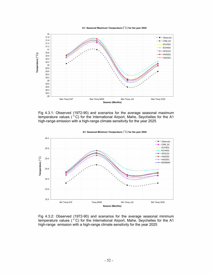
- 52 -
Fig 4.3.1: Observed (1972-90) and scenarios for the average seasonal maximum temperature values ( o C) for the International Airport, Mahe, Seychelles for the A1 high-range emission with a high-range climate sensitivity for the year 2025
Fig 4.3.2: Observed (1972-90) and scenarios for the average seasonal minimum temperature values ( o C) for the International Airport, Mahe, Seychelles for the A1 high-range emission with a high-range climate sensitivity for the year 2025
A1: Seasonal Maximum Temperature (o C) for the year 2025
28 28.2 28.4 28.6 28.8
29 29.2 29.4 29.6 29.8
30 30.2 30.4 30.6 30.8
31 31.2 31.4 31.6 31.8
32
Max Temp DJF Max Temp MAM Max Temp JJA Max Temp SON Season (Months)
Observed
CSM_D2
ECH3D2
ECH4D2
GFDLD2
HAD2D2
HAD3D2
A1: Seasonal Minimum Temperature (o C) for the year 2025
23.4
23.9
24.4
24.9
25.4
25.9
26.4
Min Temp DJF Temp MAM Min Temp JJA Min Temp SON Season (Months)
Tem
pera
ture
(o C
)
Observed CSM_D2 ECH3D2 ECH4D2 GFDLD2 HAD2D2 HAD3D2 MODBAR
Tem
pera
ture
(o C
))
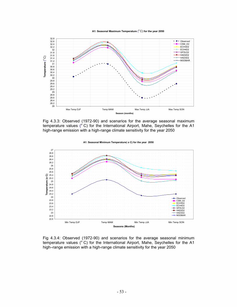
- 53 -
Fig 4.3.3: Observed (1972-90) and scenarios for the average seasonal maximum temperature values (o C) for the International Airport, Mahe, Seychelles for the A1 high-range emission with a high-range climate sensitivity for the year 2050
A1: Seasonal Minimum Temperature( o C) for the year 2050
22.622.8
2323.223.423.623.8
2424.224.424.624.8
2525.225.425.625.8
2626.226.426.626.8
27
Min Temp DJF Temp MAM Min Temp JJA Min Temp SON
Seasons (Months)
Tem
pera
ture
(o C
)
ObservedCSM_D2ECH3D2ECH4D2GFDLD2HAD2D2HAD3D2MODBAR
Fig 4.3.4: Observed (1972-90) and scenarios for the average seasonal minimum temperature values (o C) for the International Airport, Mahe, Seychelles for the A1 high–range emission with a high-range climate sensitivity for the year 2050
A1: Seasonal Maximum Temperature (o C) for the year 2050
28 28.2 28.4 28.6 28.8 29 29.2 29.4 29.6 29.8 30 30.2 30.4 30.6 30.8 31 31.2 31.4 31.6 31.8 32 32.2 32.4 32.6 32.8
Max Temp DJF Temp MAM Max Temp JJA Max Temp SON Season (months)
Observed CSM_D2 ECH3D2 ECH4D2 GFDLD2 HAD2D2 HAD3D2 MODBAR
Tem
pera
ture
(o C
)
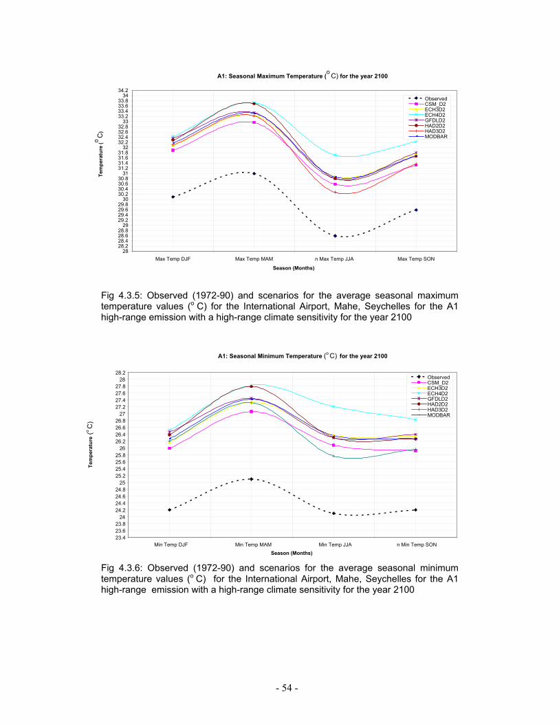
- 54 -
Fig 4.3.5: Observed (1972-90) and scenarios for the average seasonal maximum temperature values (o C) for the International Airport, Mahe, Seychelles for the A1 high-range emission with a high-range climate sensitivity for the year 2100
Fig 4.3.6: Observed (1972-90) and scenarios for the average seasonal minimum temperature values (o C) for the International Airport, Mahe, Seychelles for the A1 high-range emission with a high-range climate sensitivity for the year 2100
A1: Seasonal Maximum Temperature (o C) for the year 2100
28 28.2 28.4 28.6 28.8 29 29.2 29.4 29.6 29.8 30 30.2 30.4 30.6 30.8 31 31.2 31.4 31.6 31.8 32 32.2 32.4 32.6 32.8 33 33.2 33.4 33.6 33.8 34 34.2
Max Temp DJF Max Temp MAM n Max Temp JJA Max Temp SON Season (Months)
Observed CSM_D2 ECH3D2 ECH4D2 GFDLD2 HAD2D2 HAD3D2 MODBAR
A1: Seasonal Minimum Temperature (o C) for the year 2100
23.4 23.6 23.8
24 24.2 24.4 24.6 24.8
25 25.2 25.4 25.6 25.8
26 26.2 26.4 26.6 26.8
27 27.2 27.4 27.6 27.8
28 28.2
Min Temp DJF Min Temp MAM Min Temp JJA n Min Temp SON Season (Months)
ObservedCSM_D2 ECH3D2 ECH4D2 GFDLD2 HAD2D2 HAD3D2 MODBAR
Tem
pera
ture
(o C
) Te
mpe
ratu
re (o
C)
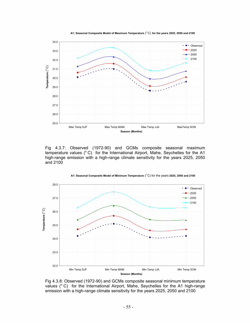
- 55 -
Fig 4.3.7: Observed (1972-90) and GCMs composite seasonal maximum temperature values (o C) for the International Airport, Mahe, Seychelles for the A1 high-range emission with a high-range climate sensitivity for the years 2025, 2050 and 2100
Fig 4.3.8: Observed (1972-90) and GCMs composite seasonal minimum temperature values (o C) for the International Airport, Mahe, Seychelles for the A1 high-range emission with a high-range climate sensitivity for the years 2025, 2050 and 2100
A1: Seasonal Composite Model of Maximum Temperature (o C) for the years 2025, 2050 and 2100
25.0
26.0
27.0
28.0
29.0
30.0
31.0
32.0
33.0
34.0
Max Temp DJF Max Temp MAM Max Temp JJA MaxTemp SON Season (Months)
Observed2025 2050 2100
A1: Seasonal Composite Model of Minimum Temperature (o C) for the years 2025, 2050 and 2100
22.0
23.0
24.0
25.0
26.0
27.0
28.0
Min Temp DJF Min Temp MAM Min Temp JJA Min Temp SON Season (Months)
Observed
2025 2050 2100
Tem
pera
ture
(o C
) Te
mpe
ratu
re (o
C)
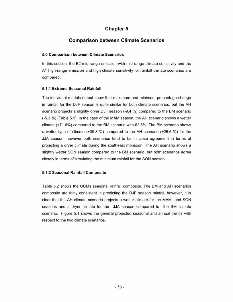
- 56 -
Chapter 5
Comparison between Climate Scenarios 5.0 Comparison between Climate Scenarios In this section, the B2 mid-range emission with mid-range climate sensitivity and the
A1 high-range emission and high climate sensitivity for rainfall climate scenarios are
compared.
5.1.1 Extreme Seasonal Rainfall The individual models output show that maximum and minimum percentage change
in rainfall for the DJF season is quite similar for both climate scenarios, but the AH
scenario projects a slightly dryer DJF season (-9.4 %) compared to the BM scenario
(-5.3 %) (Table 5.1). In the case of the MAM season, the AH scenario shows a wetter
climate (+71.6%) compared to the BM scenario with 62.8%. The BM scenario shows
a wetter type of climate (+39.8 %) compared to the AH scenario (+25.6 %) for the
JJA season, however both scenarios tend to be in close agreement in terms of
projecting a dryer climate during the southeast monsoon. The AH scenario shows a
slightly wetter SON season compared to the BM scenario, but both scenarios agree
closely in terms of simulating the minimum rainfall for the SON season.
5.1.2 Seasonal Rainfall Composite Table 5.2 shows the GCMs seasonal rainfall composite. The BM and AH scenarios
composite are fairly consistent in predicting the DJF season rainfall, however, it is
clear that the AH climate scenario projects a wetter climate for the MAM and SON
seasons and a dryer climate for the JJA season compared to the BM climate
scenario. Figure 5.1 shows the general projected seasonal and annual trends with
respect to the two climate scenarios.
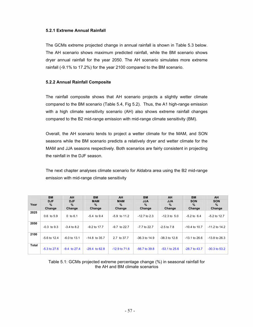
- 57 -
5.2.1 Extreme Annual Rainfall The GCMs extreme projected change in annual rainfall is shown in Table 5.3 below.
The AH scenario shows maximum predicted rainfall, while the BM scenario shows
dryer annual rainfall for the year 2050. The AH scenario simulates more extreme
rainfall (-9.1% to 17.2%) for the year 2100 compared to the BM scenario.
5.2.2 Annual Rainfall Composite
The rainfall composite shows that AH scenario projects a slightly wetter climate
compared to the BM scenario (Table 5.4, Fig 5.2). Thus, the A1 high-range emission
with a high climate sensitivity scenario (AH) also shows extreme rainfall changes
compared to the B2 mid-range emission with mid-range climate sensitivity (BM).
Overall, the AH scenario tends to project a wetter climate for the MAM, and SON
seasons while the BM scenario predicts a relatively dryer and wetter climate for the
MAM and JJA seasons respectively. Both scenarios are fairly consistent in projecting
the rainfall in the DJF season.
The next chapter analyses climate scenario for Aldabra area using the B2 mid-range
emission with mid-range climate sensitivity
BM AH BM AH BM AH BM AH
Year
DJF %
Change
DJF %
Change
MAM %
Change
MAM %
Change
JJA %
Change
JJA %
Change
SON %
Change
SON %
Change 2025
0.6 to 5.9 0 to 6.1 -5.4 to 9.4 -5.9 to 11.2 -12.7 to 2.3
-12.3 to 5.0
-5.2 to 6.4 -5.2 to 12.7
2050 -0.3 to 9.3 -3.4 to 8.2 -9.2 to 17.7 -9.7 to 22.7 -7.7 to 22.7
-2.5 to 7.8
-10.4 to 10.7 -11.2 to 14.2
2100 -5.6 to 12.4 -6.0 to 13.1 -14.8 to 35.7 2.7 to 37.7 -36.3 to 14.9
-38.3 to 12.8
-13.1 to 26.6 -13.8 to 26.3
Total -5.3 to 27.6 -9.4 to 27.4 -29.4 to 62.8 -12.9 to 71.6 -56.7 to 39.8
-53.1 to 25.6
-28.7 to 43.7 -30.3 to 53.2
Table 5.1: GCMs projected extreme percentage change (%) in seasonal rainfall for
the AH and BM climate scenarios

- 58 -
BM AH BM AH BM AH BM AH Year
DJF %
Change
DJF %
Change
MAM %
Change
MAM %
Change
JJA %
Change
JJA %
Change
SON %
Change
SON %
Change 2025 3.7 3.6 2.0 2.7 -3.3
-3.7 3.8 8.0
2050 5.3 3.4 4.3 6.6 7.3 -8.7 2.4 4.8
2100 4.9 5.2 10.5 15.6 -10.8 -14.4 11.8 12.5
Total 13.9 12.2 16.8 24.9 -6.8 -26.8 18.0 25.3
Table 5.2: GCMs projected composite percentage change (%) in seasonal rainfall
with AH and BM climate scenarios.
Year
BM
% Change in Rainfall
AH
% change in Rainfall
2025 -2.0 to 6.4
-2.0 to 6.4
2050 -4.8 to 8.5 2.3 to 9.7
2100 -8.6 to 16.3 -9.1 to 17.2
Table 5.3: GCMs projected extreme percentage change (%) in annual rainfall with
AH and BM climate scenarios
Year
BM
% change in Rainfall
AH
% change in Rainfall
2025
2.8
2.8
2050
2.7
4.6
2100 5.4
5.8
Table 5.4: GCMs projected composite percentage change (%) in annual rainfall with
AH and BM climate scenarios
- 59 -
-30
-25
-20
-15
-10
-5
0
5
10
15
20
25
30
BM(DJF) AH(DJF) BM(MAM) AH(MAM) BM(JJA) AH(JJA) BM(SON) AH(SON)
Climate Scenario and Season
Com
posi
te %
Cha
nge
in S
easo
nal R
ainf
all
2025
2050
2100
Total
Fig 5.1: GCMs projected composite percentage change (%) in seasonal rainfall with
AH and BM climate scenarios.
0
2
4
6
8
10
12
14
BM AH
Climate Scenario
Com
posi
te %
cha
nge
in A
nnua
l Rai
nfal
l
2025
2050
2100
Total
Fig 5.2: GCMs projected composite percentage change (%) in annual rainfall with AH
and BM climate scenarios .
- 60 -
Chapter 6
Climate Changes for Aldabra Group- B2 Mid-Range Emission with Mid-Range Climate Sensitivity
6.0 Climate Changes for Aldabra Group- B2 Mid-Range Emission with Mid-Range Climate Sensitivity (BM) 6.1.1 Spatial Rainfall Changes The GCMs spatial percentage change in rainfall in the case of the BM scenario for
Aldabra area are shown in Figure 6.1 for the DJF and the JJA seasons only. It also
includes the annual percentage precipitation changes. In principle, one can apply the
percentage change to any rainfall data located within the defined boundary (Fig 1b).
However, in this section, only the percentage change in rainfall is analyzed.
The spatial graphical output shows positive, wetter-like climate changes for the DJF
season while much anticipated negative, dryer –like climate for the JJA season. The
percentage change in annual rainfall is not significant. The wet and the drying spatial
changes seems to suggest dryer and wetter conditions by the year 2100.The
SCENGEN output files are therefore analyzed for further details. Table 6.1, shows
the detailed statistics for the Aldabra climate scenario for the DJF and the JJA
seasons and the annual percent change in rainfall.
6.1.2 Extremes of Seasonal rainfall
The individual GCM projected change in seasonal rainfall for the DJF season show a
minimum of -0.3 % and a maximum change of +7.2 % in rainfall for the year 2025.
The lowest change in predicted rainfall is -1.1% while the maximum change is
+12.6 % for the year 2050 and -6.2 %, +19.5 % for the year 2100.On the other hand,
the GCMs individual projections for the JJA season shows consistent negative
change in rainfall from -1.9 % to -17.4 % for the year 2025, -1.9 % to -30.1 % for the
year 2050 and 8.1 %, to -44.6 % for the year 2100. Figures 6.1.1 to 6.1.3 show the
GCMs rainfall projections for years 2025, 2050 and 2100.
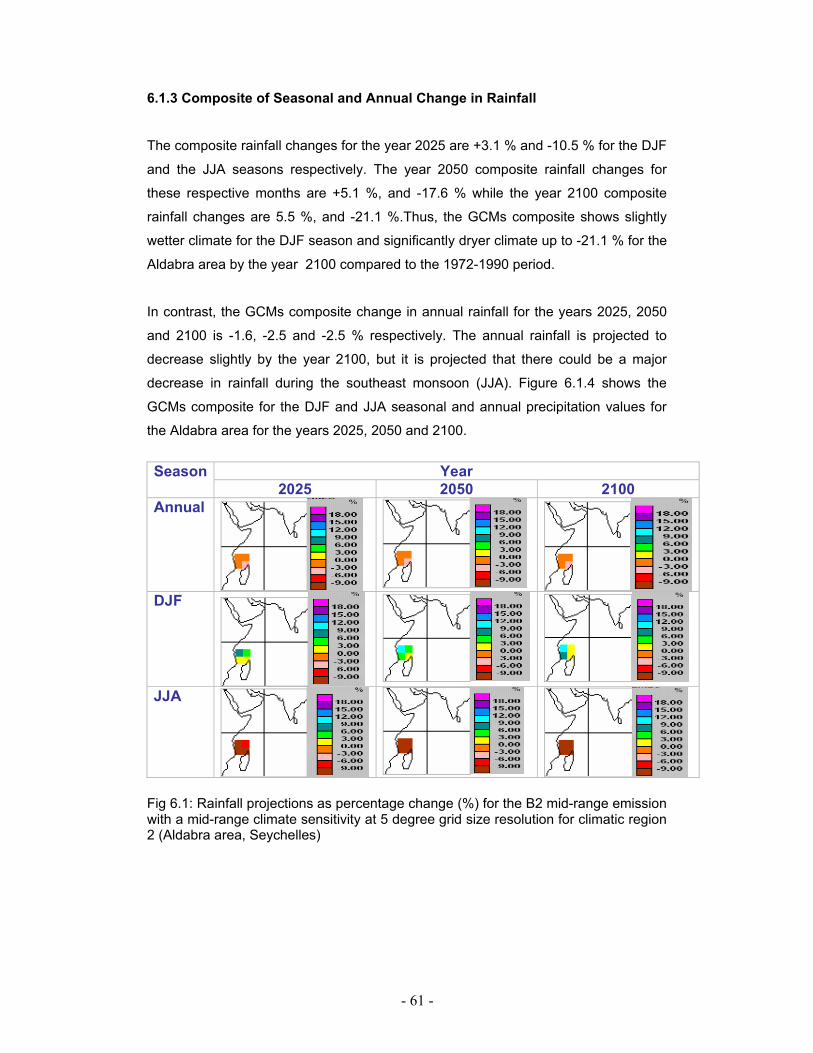
- 61 -
6.1.3 Composite of Seasonal and Annual Change in Rainfall
The composite rainfall changes for the year 2025 are +3.1 % and -10.5 % for the DJF
and the JJA seasons respectively. The year 2050 composite rainfall changes for
these respective months are +5.1 %, and -17.6 % while the year 2100 composite
rainfall changes are 5.5 %, and -21.1 %.Thus, the GCMs composite shows slightly
wetter climate for the DJF season and significantly dryer climate up to -21.1 % for the
Aldabra area by the year 2100 compared to the 1972-1990 period.
In contrast, the GCMs composite change in annual rainfall for the years 2025, 2050
and 2100 is -1.6, -2.5 and -2.5 % respectively. The annual rainfall is projected to
decrease slightly by the year 2100, but it is projected that there could be a major
decrease in rainfall during the southeast monsoon (JJA). Figure 6.1.4 shows the
GCMs composite for the DJF and JJA seasonal and annual precipitation values for
the Aldabra area for the years 2025, 2050 and 2100.
Year Season
2025 2050 2100 Annual
DJF
JJA
Fig 6.1: Rainfall projections as percentage change (%) for the B2 mid-range emission with a mid-range climate sensitivity at 5 degree grid size resolution for climatic region 2 (Aldabra area, Seychelles)
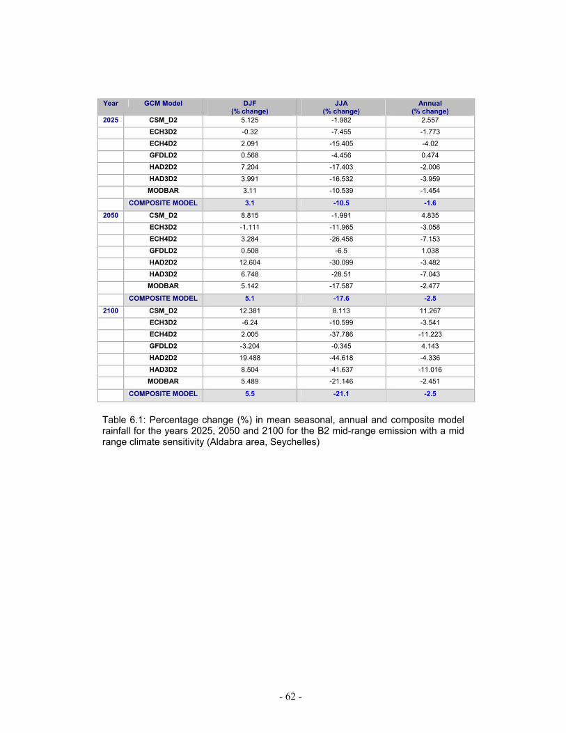
- 62 -
Year GCM Model DJF
(% change) JJA
(% change) Annual
(% change) 2025 CSM_D2 5.125 -1.982 2.557
ECH3D2 -0.32 -7.455 -1.773
ECH4D2 2.091 -15.405 -4.02
GFDLD2 0.568 -4.456 0.474
HAD2D2 7.204 -17.403 -2.006
HAD3D2 3.991 -16.532 -3.959
MODBAR 3.11 -10.539 -1.454
COMPOSITE MODEL 3.1 -10.5 -1.6
2050 CSM_D2 8.815 -1.991 4.835
ECH3D2 -1.111 -11.965 -3.058
ECH4D2 3.284 -26.458 -7.153
GFDLD2 0.508 -6.5 1.038
HAD2D2 12.604 -30.099 -3.482
HAD3D2 6.748 -28.51 -7.043
MODBAR 5.142 -17.587 -2.477
COMPOSITE MODEL 5.1 -17.6 -2.5
2100 CSM_D2 12.381 8.113 11.267
ECH3D2 -6.24 -10.599 -3.541
ECH4D2 2.005 -37.786 -11.223
GFDLD2 -3.204 -0.345 4.143
HAD2D2 19.488 -44.618 -4.336
HAD3D2 8.504 -41.637 -11.016
MODBAR 5.489 -21.146 -2.451
COMPOSITE MODEL 5.5 -21.1 -2.5
Table 6.1: Percentage change (%) in mean seasonal, annual and composite model rainfall for the years 2025, 2050 and 2100 for the B2 mid-range emission with a mid range climate sensitivity (Aldabra area, Seychelles)
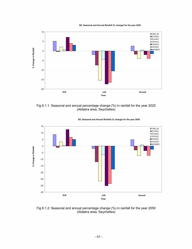
- 63 -
Fig 6.1.1: Seasonal and annual percentage change (%) in rainfall for the year 2025 (Aldabra area, Seychelles)
Fig 6.1.2: Seasonal and annual percentage change (%) in rainfall for the year 2050 (Aldabra area, Seychelles)
B2: Seasonal and Annual Rainfall (% change) for the year 2025
-20
-15
-10
-5
0
5
10
DJF JJA Annual Time
CSM_D2ECH3D2ECH4D2GFDLD2HAD2D2HAD3D2MODBAR
B2: Seasonal and Annual Rainfall (% change) for the year 2050
-35
-30
-25
-20
-15
-10
-5
0
5
10
15
DJF JJA Annual Time
CSM_D2ECH3D2ECH4D2GFDLD2HAD2D2HAD3D2MODBAR
% C
hang
e in
Rai
nfal
l %
Cha
nge
in R
ainf
all
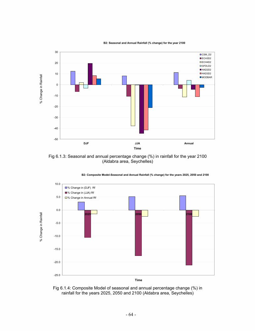
- 64 -
Fig 6.1.3: Seasonal and annual percentage change (%) in rainfall for the year 2100
(Aldabra area, Seychelles)
Fig 6.1.4: Composite Model of seasonal and annual percentage change (%) in
rainfall for the years 2025, 2050 and 2100 (Aldabra area, Seychelles)
B2: Seasonal and Annual Rainfall (% change) for the year 2100
-50
-40
-30
-20
-10
0
10
20
30
DJF JJA Annual
Time
CSM_D2ECH3D2ECH4D2GFDLD2HAD2D2HAD3D2MODBAR
B2: Composite Model-Seasonal and Annual Rainfall (% change) for the years 2025, 2050 and 2100
-25.0
-20.0
-15.0
-10.0
-5.0
0.0
5.0
10.0
2025 2050 2100
Time
% Change in (DJF) Rf % Change in (JJA) Rf % Change in Annual Rf
% C
hang
e in
Rai
nfal
l %
Cha
nge
in R
ainf
all
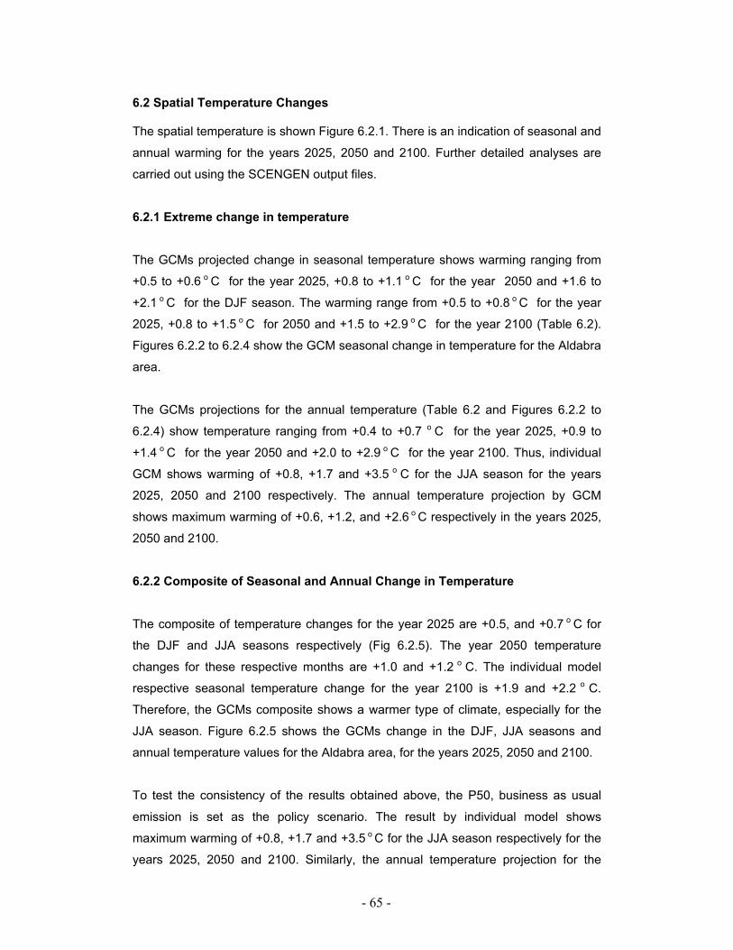
- 65 -
6.2 Spatial Temperature Changes The spatial temperature is shown Figure 6.2.1. There is an indication of seasonal and
annual warming for the years 2025, 2050 and 2100. Further detailed analyses are
carried out using the SCENGEN output files.
6.2.1 Extreme change in temperature
The GCMs projected change in seasonal temperature shows warming ranging from
+0.5 to +0.6 o C for the year 2025, +0.8 to +1.1 o C for the year 2050 and +1.6 to
+2.1 o C for the DJF season. The warming range from +0.5 to +0.8 o C for the year
2025, +0.8 to +1.5 o C for 2050 and +1.5 to +2.9 o C for the year 2100 (Table 6.2).
Figures 6.2.2 to 6.2.4 show the GCM seasonal change in temperature for the Aldabra
area.
The GCMs projections for the annual temperature (Table 6.2 and Figures 6.2.2 to
6.2.4) show temperature ranging from +0.4 to +0.7 o C for the year 2025, +0.9 to
+1.4 o C for the year 2050 and +2.0 to +2.9 o C for the year 2100. Thus, individual
GCM shows warming of +0.8, +1.7 and +3.5 o C for the JJA season for the years
2025, 2050 and 2100 respectively. The annual temperature projection by GCM
shows maximum warming of +0.6, +1.2, and +2.6 o C respectively in the years 2025,
2050 and 2100.
6.2.2 Composite of Seasonal and Annual Change in Temperature
The composite of temperature changes for the year 2025 are +0.5, and +0.7 o C for
the DJF and JJA seasons respectively (Fig 6.2.5). The year 2050 temperature
changes for these respective months are +1.0 and +1.2 o C. The individual model
respective seasonal temperature change for the year 2100 is +1.9 and +2.2 o C.
Therefore, the GCMs composite shows a warmer type of climate, especially for the
JJA season. Figure 6.2.5 shows the GCMs change in the DJF, JJA seasons and
annual temperature values for the Aldabra area, for the years 2025, 2050 and 2100.
To test the consistency of the results obtained above, the P50, business as usual
emission is set as the policy scenario. The result by individual model shows
maximum warming of +0.8, +1.7 and +3.5 o C for the JJA season respectively for the
years 2025, 2050 and 2100. Similarly, the annual temperature projection for the
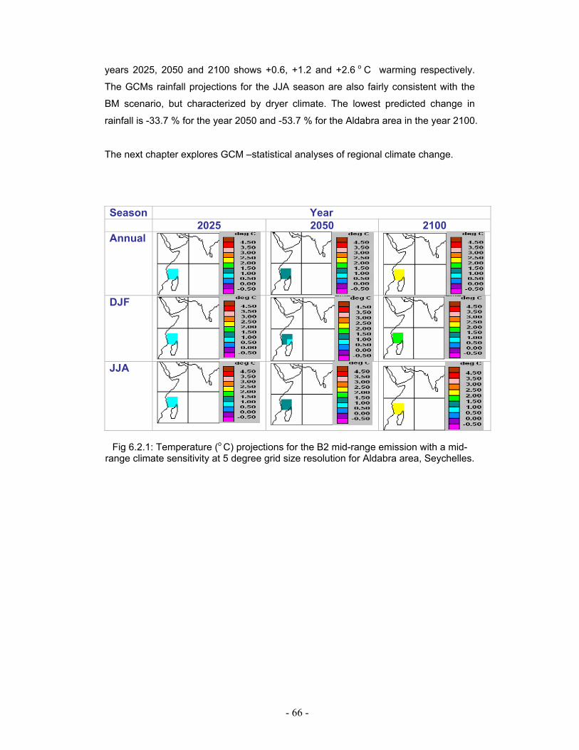
- 66 -
years 2025, 2050 and 2100 shows +0.6, +1.2 and +2.6 o C warming respectively.
The GCMs rainfall projections for the JJA season are also fairly consistent with the
BM scenario, but characterized by dryer climate. The lowest predicted change in
rainfall is -33.7 % for the year 2050 and -53.7 % for the Aldabra area in the year 2100.
The next chapter explores GCM –statistical analyses of regional climate change.
Season Year 2025 2050 2100 Annual
DJF
JJA
Fig 6.2.1: Temperature (o C) projections for the B2 mid-range emission with a mid-range climate sensitivity at 5 degree grid size resolution for Aldabra area, Seychelles.
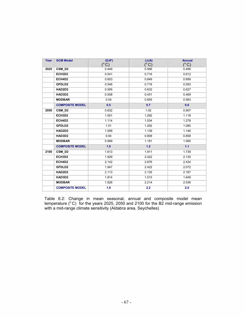
- 67 -
Year GCM Model (DJF)
(o C) (JJA) (o C)
Annual (o C)
2025 CSM_D2 0.449 0.566 0.496
ECH3D2 0.541 0.716 0.612
ECH4D2 0.603 0.849 0.699
GFDLD2 0.546 0.716 0.593
HAD2D2 0.595 0.632 0.627
HAD3D2 0.508 0.451 0.469
MODBAR 0.54 0.655 0.583
COMPOSITE MODEL 0.5 0.7 0.6
2050 CSM_D2 0.832 1.02 0.907
ECH3D2 1.001 1.292 1.118
ECH4D2 1.114 1.534 1.278
GFDLD2 1.01 1.292 1.085
HAD2D2 1.099 1.139 1.146
HAD3D2 0.94 0.809 0.858
MODBAR 0.999 1.181 1.065
COMPOSITE MODEL 1.0 1.2 1.1
2100 CSM_D2 1.613 1.911 1.739
ECH3D2 1.929 2.422 2.135
ECH4D2 2.142 2.876 2.434
GFDLD2 1.947 2.422 2.072
HAD2D2 2.113 2.135 2.187
HAD3D2 1.814 1.515 1.648
MODBAR 1.926 2.214 2.036
COMPOSITE MODEL 1.9 2.2 2.0
Table 6.2: Change in mean seasonal, annual and composite model mean temperature (o C) for the years 2025, 2050 and 2100 for the B2 mid-range emission with a mid-range climate sensitivity (Aldabra area, Seychelles)
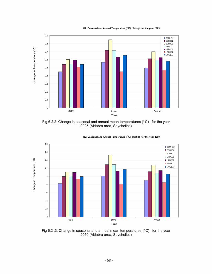
- 68 -
Fig 6.2.2: Change in seasonal and annual mean temperatures (o C) for the year
2025 (Aldabra area, Seychelles)
Fig 6.2 .3: Change in seasonal and annual mean temperatures (o C) for the year
2050 (Aldabra area, Seychelles)
B2: Seasonal and Annual Temperature (o C) change for the year 2025
0
0.1
0.2
0.3
0.4
0.5
0.6
0.7
0.8
0.9
(DJF) (JJA) Annual Time
CSM_D2ECH3D2ECH4D2GFDLD2HAD2D2HAD3D2MODBAR
B2: Seasonal and Annual Temperature (o C) change for the year 2050
0
0.2
0.4
0.6
0.8
1
1.2
1.4
1.6
1.8
(DJF) (JJA) Annual Time
CSM_D2
ECH3D2
ECH4D2
GFDLD2
HAD2D2
HAD3D2
MODBAR
Cha
nge
in T
empe
ratu
re (o
C)
Cha
nge
in T
empe
ratu
re (o
C)
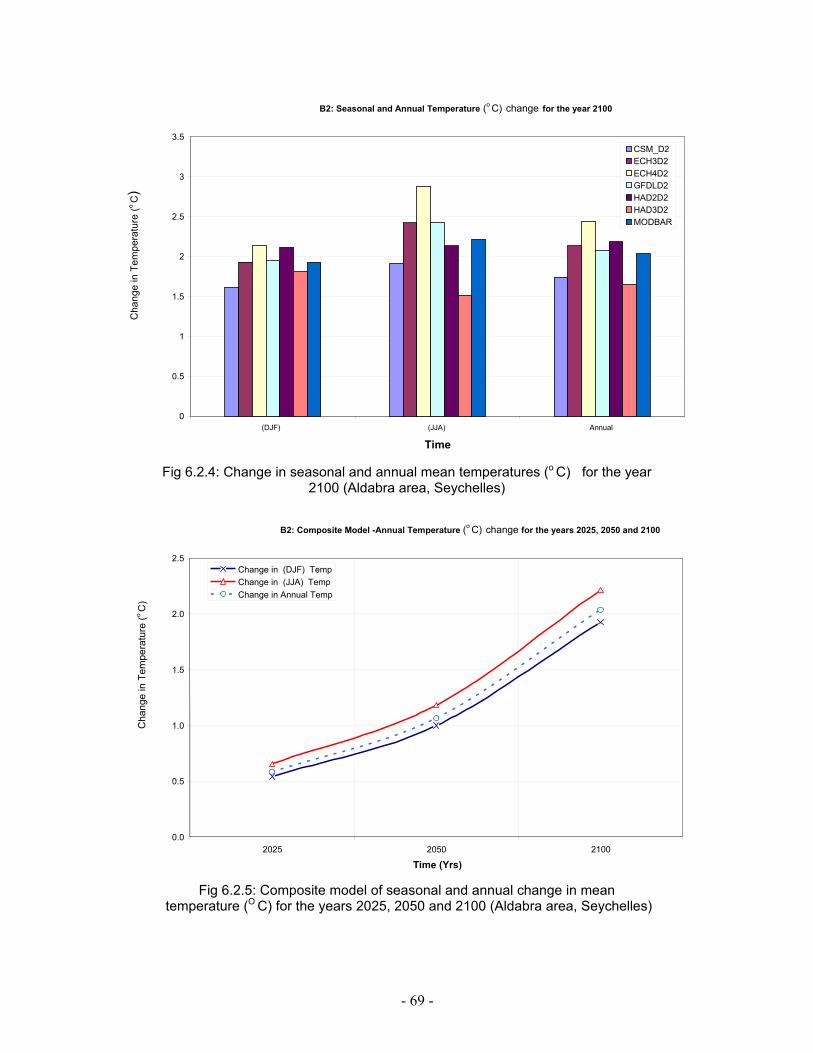
- 69 -
Fig 6.2.4: Change in seasonal and annual mean temperatures (o C) for the year
2100 (Aldabra area, Seychelles)
Fig 6.2.5: Composite model of seasonal and annual change in mean
temperature (O C) for the years 2025, 2050 and 2100 (Aldabra area, Seychelles)
B2: Seasonal and Annual Temperature (o C) change for the year 2100
0
0.5
1
1.5
2
2.5
3
3.5
(DJF) (JJA) Annual Time
CSM_D2ECH3D2ECH4D2GFDLD2HAD2D2HAD3D2MODBAR
B2: Composite Model -Annual Temperature (o C) change for the years 2025, 2050 and 2100
0.0
0.5
1.0
1.5
2.0
2.5
2025 2050 2100 Time (Yrs)
Change in (DJF) TempChange in (JJA) TempChange in Annual Temp
Cha
nge
in T
empe
ratu
re (o
C)
C
hang
e in
Tem
pera
ture
(o C
)
- 70 -
Chapter 7
General Circulation Model (GCM) and Statistical Regional Climate Change
7.0 GCM and Statistical Regional Climate Change In this section, the GCM-Guided Perturbation Method (GPM) for regional climate
change scenarios developed by Hewitson, University of Cape Town and the Regional
Climate-Change Projection from Multi-Model Ensembles (RCPM) developed by the
National Center for Atmospheric Research (NCAR) and the University Corporation
for Atmospheric Research (UCAR) are investigated as other possible results for
integration in the assessment.
7.1 GCM-Guided Perturbation Method (GPM) for Regional Climate Change 7.1.1 Rainfall changes GPM is not a GCM downscaled methodology, but it does represent a regional scale
perturbation in accord with the GCM first order response to greenhouse gas forcing.
Consequently, this allows one to undertake an assessment of fundamental regional
sensitivities to climate change, in a manner that is not arbitrary, but guided by GCMs.
The climate scenario selected is for the A2 and B2 emission scenario. The GCMS
are also slightly different. The time resolution is at a monthly time scale. Only the
results for the year 2100 are presented here. The overall objective is to explore
differences in the climate trends. Figure 7.1 shows the A2 GCMs monthly rainfall for
the year 2100. The NACR-CSM GCM-Guided Perturbation Method (GPM) shows
peak rainfall anomaly from November to February for the A2 scenario (Fig 7.1), but
for the B2 emission (Fig 7.2), the NACR-CSM model output is significantly different to
the rather constant rainfall anomaly of between 20-40 mm for all the months. In
contrast, the NACR-PCM shows peak positive rainfall anomaly in February but
gradually decreases towards December. In the case of the B2 emission scenario the
trend apparently reverses with peak rainfall in December. Overall, the NACR-PCM
and NCAR-CSM GCM-Guided Perturbation Method (GPM) show large positive
anomaly in rainfall; indicating wetter-like climate for most of the months especially
during the rainy season. The dry season is projected to be slightly wetter than normal.
Apart from the NACR-PCM and the NCAR-CSM, all the GCM-GPM tend to project
- 71 -
very small rainfall departures from the mean rainfall. The rainfall anomaly for both the
A2 and B2 scenarios between the NCAR-PSM and the NACR-CSM GCM-Guided
Perturbation Method (GPM) are found to have large deviations in predicted rainfall
compared to the other four models. It is also suspicious to observe that there is no
predicted decrease in rainfall for all the months. The GCM-GPM method portrays the
complete absence of droughts with future green house induced climate changes.
7.1.2 Temperature changes On further examination, the projected maximum and minimum temperature reveals
that the southeast monsoon (JJA) would become warmer than the northwest
monsoon (DJF), with the exception of the NACR-CSM GCM-Guided Perturbation
Method (GPM) output. The NACR-CSM GCM-Guided Perturbation Method is not
available for the B2 emission scenario. This simply implies a total shift in the
seasonal temperature patterns. However, it is unclear why the normal rainfall peaks
do not shift to be in phase with the projected seasonal thermodynamic shift. Thus,
only the output from the NACR-CSM can be considered meaningful.

- 72 -
Fig 7.1: A2 GCMs monthly rainfall anomaly (mm) for the year 2100
B2: Monthly Rainfall Anomaly (mm) for the year 2100
-20
0
20
40
60
80
100
120
140
160
JAN FEB MAR APR MAY JUN JUL AUG SEP OCT NOV DEC
Time (Months)
Rai
nfal
l Ano
mal
y (m
m)
CCCMA
CSIRO
HADCM3
ECHAM
NACAR-PCM
NACR-CSM
Fig 7.1.2: B2 GCMs monthly rainfall anomaly (mm) for the year 2100
A2: Monthly Rainfall Anomaly (mm) for the year 2100
-20
0
20
40
60
80
100
120
140
160
180
JAN FEB MAR APR MAY JUN JUL AUG SEP OCT NOV DEC
Time (Months)
CCCMA CSIRO HADCM3 ECHAM NACAR-PCM NACR-CSM
Rai
nfal
l Ano
mal
y (m
m)
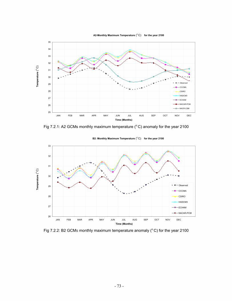
- 73 -
Fig 7.2.1: A2 GCMs monthly maximum temperature (o C) anomaly for the year 2100
Fig 7.2.2: B2 GCMS monthly maximum temperature anomaly (o C) for the year 2100
A2-Monthly Maximum Temperature (o C) for the year 2100
25 26 27 28 29 30
31 32 33 34 35
JAN FEB MAR APR MAY JUN JUL AUG SEP OCT NOV DEC
Time (Months)
Observed
CCCMA CSIRO HADCM3
ECHAM NACAR-PCM
NACR-CSM
B2: Monthly Maximum Temperature (o C) for the year 2100
26
27
28
29
30
31
32
33
JAN FEB MAR APR MAY JUN JUL AUG SEP OCT NOV DEC Time (Months)
Observed
CCCMA CSIRO HADCM3
ECHAM NACAR-PCM
Tem
pera
ture
(o C
)
Tem
pera
ture
(o C
)

- 74 -
Fig 7.2.3: A2 GCMS monthly minimum temperature anomaly (o C) for the year 2100
NACR-CSM
Tem
pera
ture
(o C
)
A2: Monthly Minimum Temperature (o C) for the year 2100
22 22 23 23 24 24 25 25 26 26 27 27 28 28 29 29
JAN FEB MAR APR MAY JUN JUL AUG SEP OCT NOV DEC Time (Months)
Temperature (o C)
Observed CCCMA CSIRO HADCM3 ECHAM NACAR-PCM
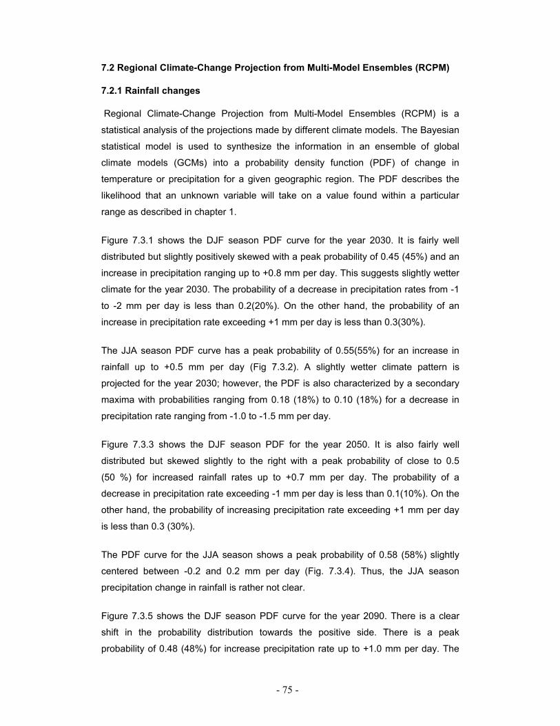
- 75 -
7.2 Regional Climate-Change Projection from Multi-Model Ensembles (RCPM)
7.2.1 Rainfall changes
Regional Climate-Change Projection from Multi-Model Ensembles (RCPM) is a
statistical analysis of the projections made by different climate models. The Bayesian
statistical model is used to synthesize the information in an ensemble of global
climate models (GCMs) into a probability density function (PDF) of change in
temperature or precipitation for a given geographic region. The PDF describes the
likelihood that an unknown variable will take on a value found within a particular
range as described in chapter 1.
Figure 7.3.1 shows the DJF season PDF curve for the year 2030. It is fairly well
distributed but slightly positively skewed with a peak probability of 0.45 (45%) and an
increase in precipitation ranging up to +0.8 mm per day. This suggests slightly wetter
climate for the year 2030. The probability of a decrease in precipitation rates from -1
to -2 mm per day is less than 0.2(20%). On the other hand, the probability of an
increase in precipitation rate exceeding +1 mm per day is less than 0.3(30%).
The JJA season PDF curve has a peak probability of 0.55(55%) for an increase in
rainfall up to +0.5 mm per day (Fig 7.3.2). A slightly wetter climate pattern is
projected for the year 2030; however, the PDF is also characterized by a secondary
maxima with probabilities ranging from 0.18 (18%) to 0.10 (18%) for a decrease in
precipitation rate ranging from -1.0 to -1.5 mm per day.
Figure 7.3.3 shows the DJF season PDF for the year 2050. It is also fairly well
distributed but skewed slightly to the right with a peak probability of close to 0.5
(50 %) for increased rainfall rates up to +0.7 mm per day. The probability of a
decrease in precipitation rate exceeding -1 mm per day is less than 0.1(10%). On the
other hand, the probability of increasing precipitation rate exceeding +1 mm per day
is less than 0.3 (30%).
The PDF curve for the JJA season shows a peak probability of 0.58 (58%) slightly
centered between -0.2 and 0.2 mm per day (Fig. 7.3.4). Thus, the JJA season
precipitation change in rainfall is rather not clear.
Figure 7.3.5 shows the DJF season PDF curve for the year 2090. There is a clear
shift in the probability distribution towards the positive side. There is a peak
probability of 0.48 (48%) for increase precipitation rate up to +1.0 mm per day. The
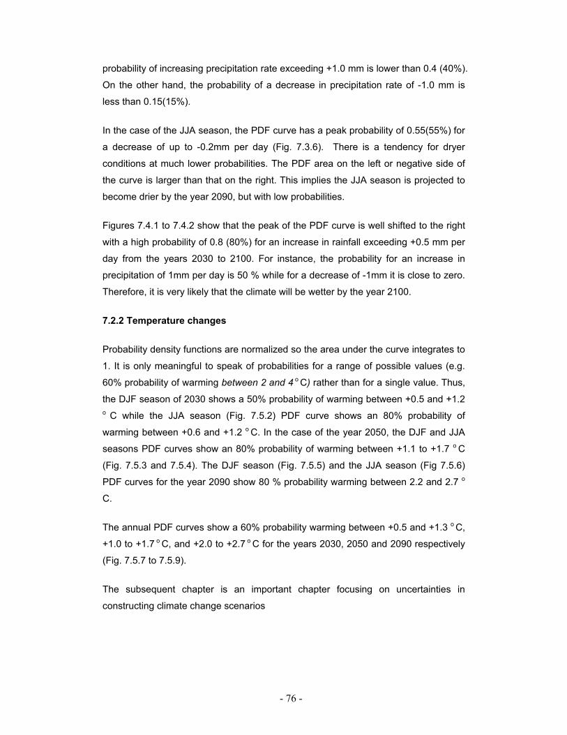
- 76 -
probability of increasing precipitation rate exceeding +1.0 mm is lower than 0.4 (40%).
On the other hand, the probability of a decrease in precipitation rate of -1.0 mm is
less than 0.15(15%).
In the case of the JJA season, the PDF curve has a peak probability of 0.55(55%) for
a decrease of up to -0.2mm per day (Fig. 7.3.6). There is a tendency for dryer
conditions at much lower probabilities. The PDF area on the left or negative side of
the curve is larger than that on the right. This implies the JJA season is projected to
become drier by the year 2090, but with low probabilities.
Figures 7.4.1 to 7.4.2 show that the peak of the PDF curve is well shifted to the right
with a high probability of 0.8 (80%) for an increase in rainfall exceeding +0.5 mm per
day from the years 2030 to 2100. For instance, the probability for an increase in
precipitation of 1mm per day is 50 % while for a decrease of -1mm it is close to zero.
Therefore, it is very likely that the climate will be wetter by the year 2100.
7.2.2 Temperature changes
Probability density functions are normalized so the area under the curve integrates to
1. It is only meaningful to speak of probabilities for a range of possible values (e.g.
60% probability of warming between 2 and 4 o C) rather than for a single value. Thus,
the DJF season of 2030 shows a 50% probability of warming between +0.5 and +1.2 o C while the JJA season (Fig. 7.5.2) PDF curve shows an 80% probability of
warming between +0.6 and +1.2 o C. In the case of the year 2050, the DJF and JJA
seasons PDF curves show an 80% probability of warming between +1.1 to +1.7 o C
(Fig. 7.5.3 and 7.5.4). The DJF season (Fig. 7.5.5) and the JJA season (Fig 7.5.6)
PDF curves for the year 2090 show 80 % probability warming between 2.2 and 2.7 o
C.
The annual PDF curves show a 60% probability warming between +0.5 and +1.3 o C,
+1.0 to +1.7 o C, and +2.0 to +2.7 o C for the years 2030, 2050 and 2090 respectively
(Fig. 7.5.7 to 7.5.9).
The subsequent chapter is an important chapter focusing on uncertainties in
constructing climate change scenarios
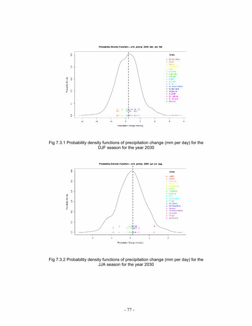
- 77 -
Fig 7.3.1 Probability density functions of precipitation change (mm per day) for the DJF season for the year 2030
Fig 7.3.2 Probability density functions of precipitation change (mm per day) for the JJA season for the year 2030
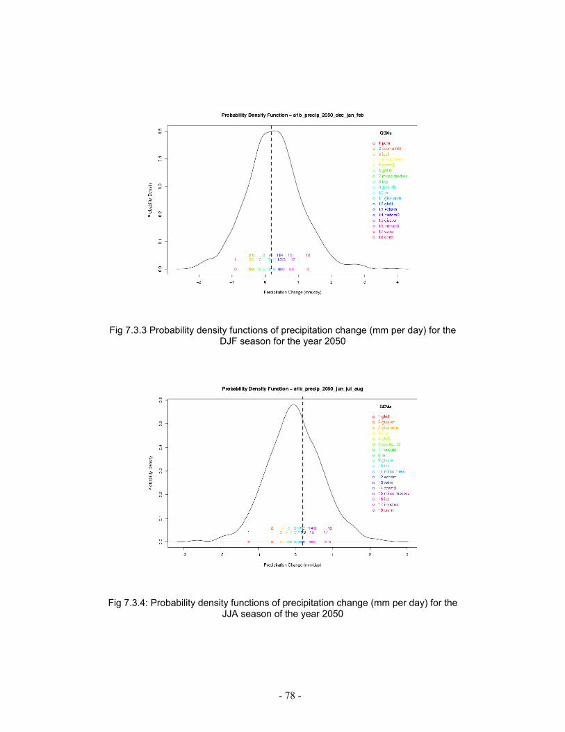
- 78 -
Fig 7.3.3 Probability density functions of precipitation change (mm per day) for the DJF season for the year 2050
Fig 7.3.4: Probability density functions of precipitation change (mm per day) for the JJA season of the year 2050
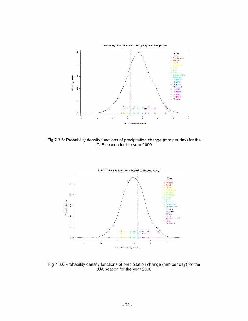
- 79 -
Fig 7.3.5: Probability density functions of precipitation change (mm per day) for the DJF season for the year 2090
Fig 7.3.6 Probability density functions of precipitation change (mm per day) for the JJA season for the year 2090
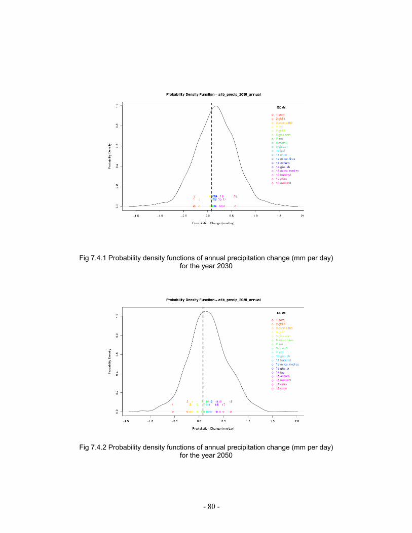
- 80 -
Fig 7.4.1 Probability density functions of annual precipitation change (mm per day) for the year 2030
Fig 7.4.2 Probability density functions of annual precipitation change (mm per day)
for the year 2050
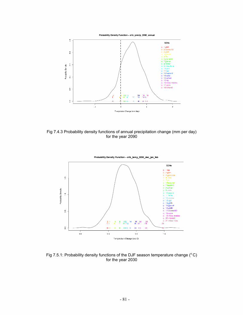
- 81 -
Fig 7.4.3 Probability density functions of annual precipitation change (mm per day)
for the year 2090
Fig 7.5.1: Probability density functions of the DJF season temperature change (o C)
for the year 2030
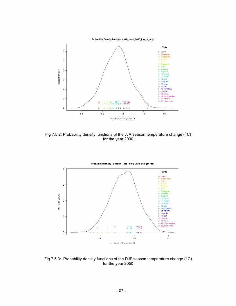
- 82 -
Fig 7.5.2: Probability density functions of the JJA season temperature change (o C) for the year 2030
Fig 7.5.3: Probability density functions of the DJF season temperature change (o C) for the year 2050

- 83 -
Fig 7.5.4: Probability density functions of the JJA season temperature change (o C)
for the year 2050
Fig 7.5.5: Probability density functions of the DJF season temperature change (o C)
for the year 2090
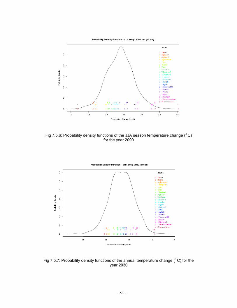
- 84 -
Fig 7.5.6: Probability density functions of the JJA season temperature change (o C) for the year 2090
Fig 7.5.7: Probability density functions of the annual temperature change (o C) for the
year 2030
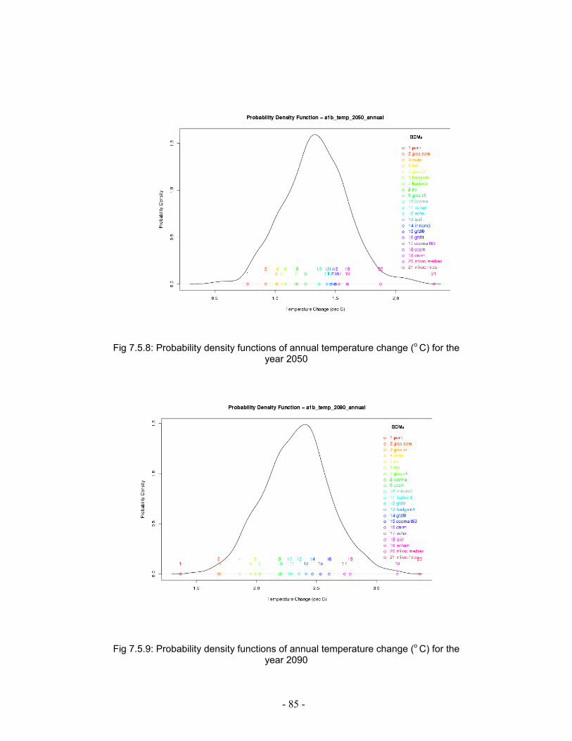
- 85 -
Fig 7.5.8: Probability density functions of annual temperature change (o C) for the year 2050
Fig 7.5.9: Probability density functions of annual temperature change (o C) for the
year 2090
- 86 -
Chapter 8
Scenario Uncertainties 8.0 Scenario Uncertainties As indicated in the previous chapters, one is able to make a number of decisions
concerning the emission scenarios, the model parameters, and the spatial pattern of
climate change used in the construction of the climate change scenarios. These
decisions will govern the magnitude, the spatial pattern and the range of climate
changes represented in the output scenarios. These options involve some of the
current uncertainties in climate change science and its prediction. The uncertainties
driving the scenarios in MAGICC /SCENGEN are the emission scenarios, the carbon
cycle, the aerosols radiative forcing, the climate sensitivity and the regional climate
change. However, in this section, emphasis is on uncertainties in regional climate
change patterns and uncertainties related to the GCM selection. It is recalled that in
chapters 2, 3 and 4 comparisons of different model results were shown for the
changes in the area patterns for seasonal and annual precipitation and temperature.
Thus, the assessment has already accounted largely for model differences in
simulating changes in area patterns. It is very important to critically look at scenario
uncertainties. Very often many fail to address and understand this scientific
component. The cost of failing to address climate scenario uncertainties obscures
our capacities to understand and respond correctly to the process. It is therefore
simply incorrect to claim that the climate will be dryer, wetter, warmer or colder
without addressing scenario uncertainties. It is noted that one of the major successes
of the IPCC Fourth Assessment Report (FAR) is its advancement in understanding
climate uncertainties. Probabilistic likelihood methods were used widely in FAR to
convey the uncertainty levels for the benefit of policy and decision makers. Therefore,
an assessment of the likelihood levels is explored. Another issue is the variability and
the divergence of climate models. As an example, policy makers are often perplexed
by the large differences between individual model climate-change results at the
regional level. Information like this can help to define adaptation strategies that are
robust to such uncertainties.
- 87 -
Thus, the following investigations are carried out to address some of the issues in a
simple but comprehensive manner:
1. To investigate changes in variability;
2. To quantify uncertainties in terms of inter-model differences;
3. To asses climate change and give probabilistic outputs.
8.1.1 Change in variability for the Mahe Area In this section the changes in variability (expressed in SCENGEN in terms of
percentage changes in inter-annual standard deviation) in the selected grid box is
investigated. This is done by averaging all models to create a composite mean (Fig
8.1.1). In summary, the percentage change in rainfall variability is -2.5 % to +2.5 %
on an annual basis, -2.5% to +10 % for the DJF season and 0 to -10 % for the JJA
season for the year 2025. The changes in rainfall variability are -5% to 10% annually,
-5 % to -15% in the DJF season and 0 to -15 % in the JJA season for the year 2050.
For the year 2100, the changes in variability are -15 % to 10 % annually, -15% to
+25% for the DJF season and 0 to -15% for the JJA season.
In simple terms, most of the cells within the selected grid box show that, on average,
changes in variability are rather small with a magnitude of less than 15% and tend
to have the same trends as found in the earlier chapters. This does not mean that
individual models all show small changes in variability (a fact that one can verify by
selecting individual models). Rather, the low variability changes arise from the fact
that different models give quite different results for the patterns of change in annual
precipitation variability, and the individual extremes tend to cancel out. Only the DJF
season of the year 2100 shows significant changes in variability which amount to
25 %. Thus, the relatively large variability of 25% suggests that models tend to
converge or agree with slightly higher confidence compared to the rest for an
increase in rainfall for the DJF season for the year 2100.

- 88 -
Year Season 2025 2050 2100
Ann
DJF
JJA
Fig 8.1.1: Change in spatial rainfall variability by season and year for the projected years 2025, 2050 and 2100 for the Mahe area The model-to-model pattern correlations for normalized variability change fields for
the selected models (variable and season) are analyzed, but not shown here. It
provides a quantitative verification of change variability. In the case of the
precipitation-change fields it is found that models do have some disagreements.
The seasonal comparison of model-to-model pattern correlations shows that the
ECH4 and the HAD3 tend to disagree with the other models. In this case negative
cross- correlations ranges between –7 and -86 %, but with mean negative value less
than 50 %. HAD2 climate model pattern is negatively correlated with the other
models, including the HAD3 at an annual time scale.
It is recalled from Tables 3.1 and 3.2 in chapters 2 and 3 that ECH3 model
consistently predicted the lowest percentage change in rainfall (+0.6 %, -0.3% and
+5.6 %) while HAD2 consistently predicted the maximum change in rainfall(+5.9 %,
+9.3 % and +12.4 % ) for the DJF season of the years 2025, 2050 and 2100
respectively. On the other hand, for the JJA season, HAD3 model frequently
predicted the lowest change in rainfall (-12.7%, -7.7% and -36.3 %) while ECH4
model predicted mostly the maximum change in rainfall (+2.3% and +14.9%) for the
years 2025 and 2100 respectively. On an annual basis, the ECH4 model predicted
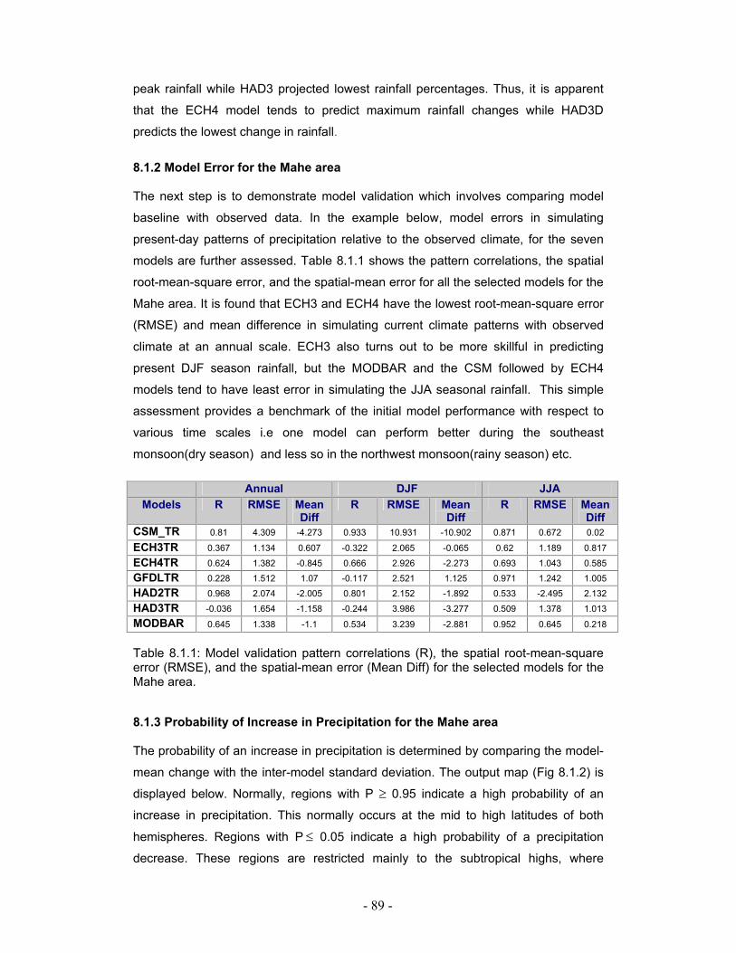
- 89 -
peak rainfall while HAD3 projected lowest rainfall percentages. Thus, it is apparent
that the ECH4 model tends to predict maximum rainfall changes while HAD3D
predicts the lowest change in rainfall.
8.1.2 Model Error for the Mahe area The next step is to demonstrate model validation which involves comparing model
baseline with observed data. In the example below, model errors in simulating
present-day patterns of precipitation relative to the observed climate, for the seven
models are further assessed. Table 8.1.1 shows the pattern correlations, the spatial
root-mean-square error, and the spatial-mean error for all the selected models for the
Mahe area. It is found that ECH3 and ECH4 have the lowest root-mean-square error
(RMSE) and mean difference in simulating current climate patterns with observed
climate at an annual scale. ECH3 also turns out to be more skillful in predicting
present DJF season rainfall, but the MODBAR and the CSM followed by ECH4
models tend to have least error in simulating the JJA seasonal rainfall. This simple
assessment provides a benchmark of the initial model performance with respect to
various time scales i.e one model can perform better during the southeast
monsoon(dry season) and less so in the northwest monsoon(rainy season) etc.
Annual DJF JJA Models R RMSE Mean
Diff R RMSE Mean
Diff R RMSE Mean
Diff CSM_TR 0.81 4.309 -4.273 0.933 10.931 -10.902 0.871 0.672 0.02
ECH3TR 0.367 1.134 0.607 -0.322 2.065 -0.065 0.62 1.189 0.817
ECH4TR 0.624 1.382 -0.845 0.666 2.926 -2.273 0.693 1.043 0.585
GFDLTR 0.228 1.512 1.07 -0.117 2.521 1.125 0.971 1.242 1.005
HAD2TR 0.968 2.074 -2.005 0.801 2.152 -1.892 0.533 -2.495 2.132
HAD3TR -0.036 1.654 -1.158 -0.244 3.986 -3.277 0.509 1.378 1.013
MODBAR 0.645 1.338 -1.1 0.534 3.239 -2.881 0.952 0.645 0.218
Table 8.1.1: Model validation pattern correlations (R), the spatial root-mean-square error (RMSE), and the spatial-mean error (Mean Diff) for the selected models for the Mahe area. 8.1.3 Probability of Increase in Precipitation for the Mahe area The probability of an increase in precipitation is determined by comparing the model-
mean change with the inter-model standard deviation. The output map (Fig 8.1.2) is
displayed below. Normally, regions with P ≥ 0.95 indicate a high probability of an
increase in precipitation. This normally occurs at the mid to high latitudes of both
hemispheres. Regions with P ≤ 0.05 indicate a high probability of a precipitation
decrease. These regions are restricted mainly to the subtropical highs, where
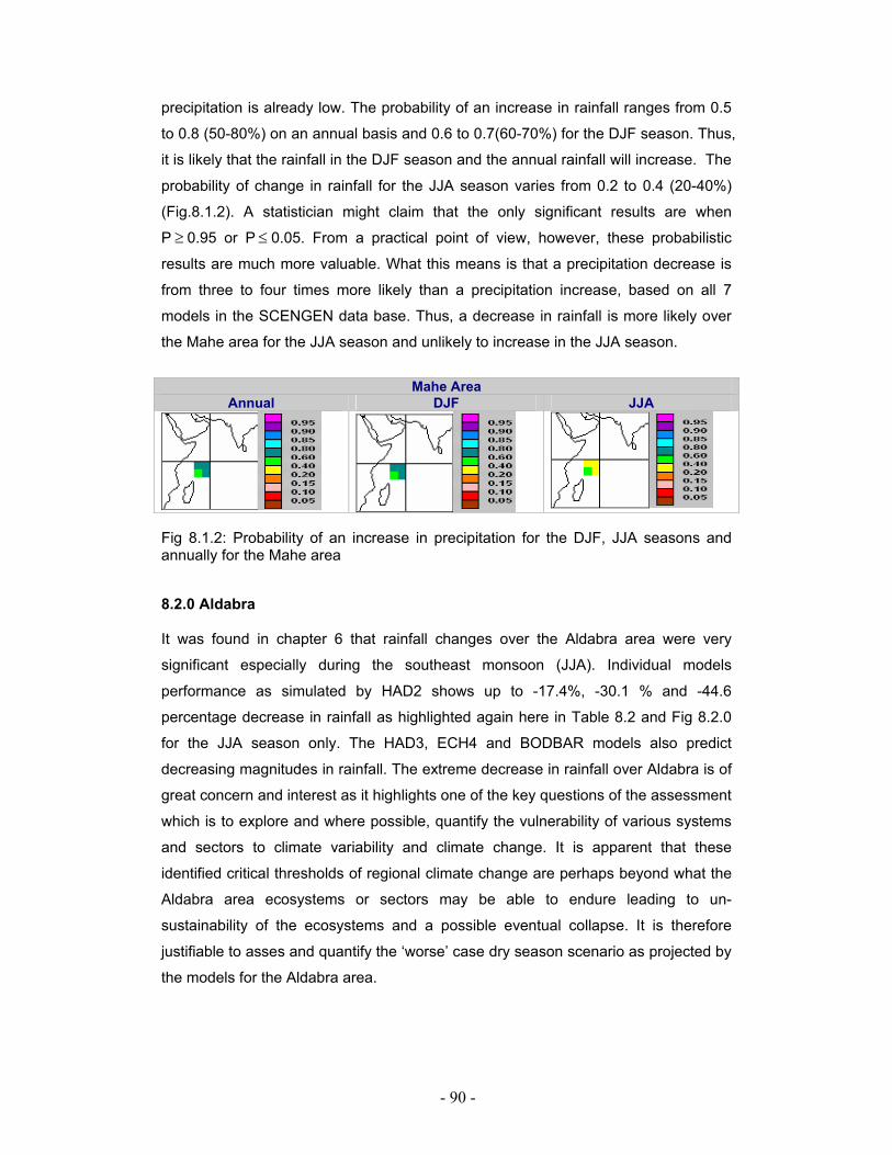
- 90 -
precipitation is already low. The probability of an increase in rainfall ranges from 0.5
to 0.8 (50-80%) on an annual basis and 0.6 to 0.7(60-70%) for the DJF season. Thus,
it is likely that the rainfall in the DJF season and the annual rainfall will increase. The
probability of change in rainfall for the JJA season varies from 0.2 to 0.4 (20-40%)
(Fig.8.1.2). A statistician might claim that the only significant results are when
P ≥ 0.95 or P ≤ 0.05. From a practical point of view, however, these probabilistic
results are much more valuable. What this means is that a precipitation decrease is
from three to four times more likely than a precipitation increase, based on all 7
models in the SCENGEN data base. Thus, a decrease in rainfall is more likely over
the Mahe area for the JJA season and unlikely to increase in the JJA season.
Mahe Area
Annual DJF JJA
Fig 8.1.2: Probability of an increase in precipitation for the DJF, JJA seasons and annually for the Mahe area 8.2.0 Aldabra It was found in chapter 6 that rainfall changes over the Aldabra area were very
significant especially during the southeast monsoon (JJA). Individual models
performance as simulated by HAD2 shows up to -17.4%, -30.1 % and -44.6
percentage decrease in rainfall as highlighted again here in Table 8.2 and Fig 8.2.0
for the JJA season only. The HAD3, ECH4 and BODBAR models also predict
decreasing magnitudes in rainfall. The extreme decrease in rainfall over Aldabra is of
great concern and interest as it highlights one of the key questions of the assessment
which is to explore and where possible, quantify the vulnerability of various systems
and sectors to climate variability and climate change. It is apparent that these
identified critical thresholds of regional climate change are perhaps beyond what the
Aldabra area ecosystems or sectors may be able to endure leading to un-
sustainability of the ecosystems and a possible eventual collapse. It is therefore
justifiable to asses and quantify the ‘worse’ case dry season scenario as projected by
the models for the Aldabra area.
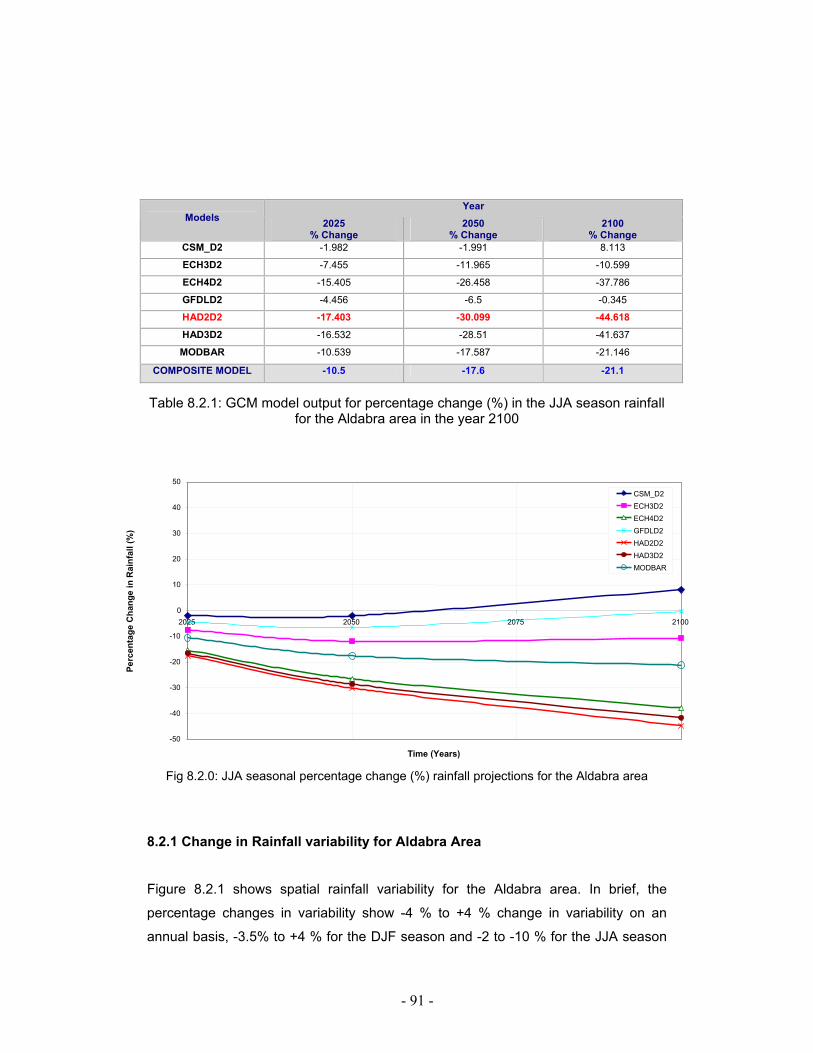
- 91 -
Year Models 2025
% Change 2050
% Change 2100
% Change CSM_D2 -1.982 -1.991 8.113
ECH3D2 -7.455 -11.965 -10.599
ECH4D2 -15.405 -26.458 -37.786
GFDLD2 -4.456 -6.5 -0.345
HAD2D2 -17.403 -30.099 -44.618
HAD3D2 -16.532 -28.51 -41.637
MODBAR -10.539 -17.587 -21.146
COMPOSITE MODEL -10.5 -17.6 -21.1
Table 8.2.1: GCM model output for percentage change (%) in the JJA season rainfall
for the Aldabra area in the year 2100
Fig 8.2.0: JJA seasonal percentage change (%) rainfall projections for the Aldabra area
8.2.1 Change in Rainfall variability for Aldabra Area Figure 8.2.1 shows spatial rainfall variability for the Aldabra area. In brief, the
percentage changes in variability show -4 % to +4 % change in variability on an
annual basis, -3.5% to +4 % for the DJF season and -2 to -10 % for the JJA season
-50
-40
-30
-20
-10
0
10
20
30
40
50
2025 2050 2075 2100
Time (Years)
CSM_D2ECH3D2ECH4D2GFDLD2HAD2D2HAD3D2MODBAR
Perc
enta
ge C
hang
e in
Rai
nfal
l (%
)
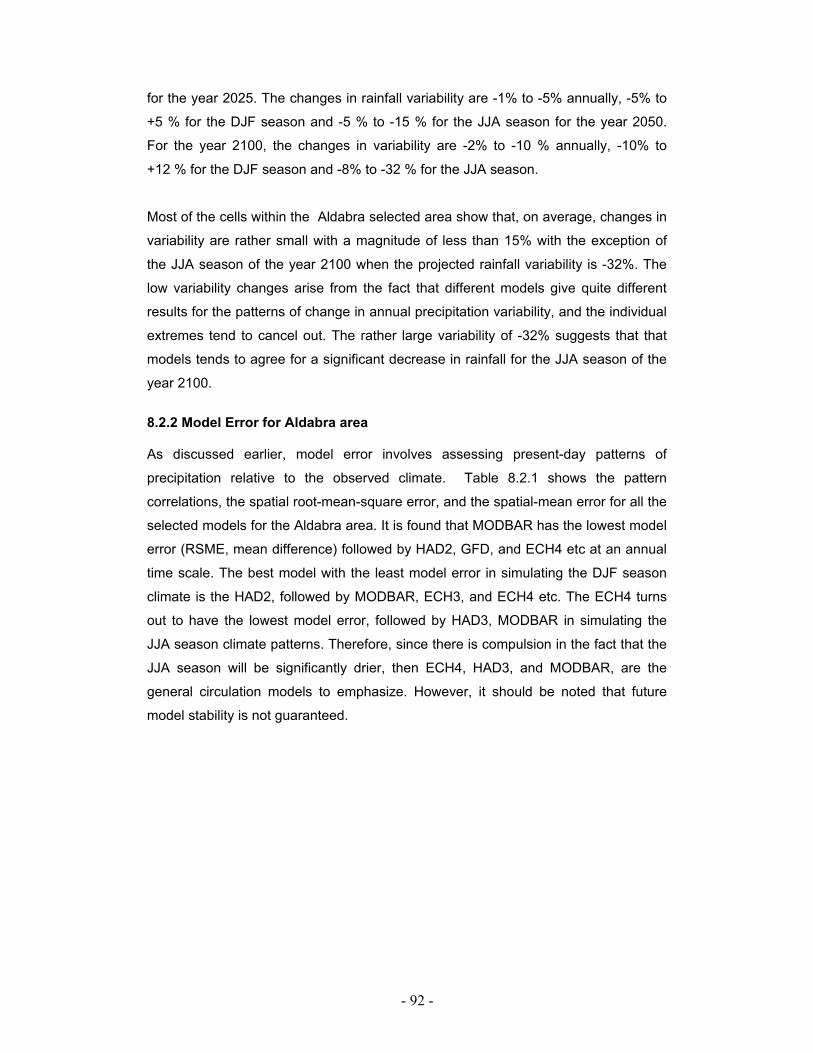
- 92 -
for the year 2025. The changes in rainfall variability are -1% to -5% annually, -5% to
+5 % for the DJF season and -5 % to -15 % for the JJA season for the year 2050.
For the year 2100, the changes in variability are -2% to -10 % annually, -10% to
+12 % for the DJF season and -8% to -32 % for the JJA season.
Most of the cells within the Aldabra selected area show that, on average, changes in
variability are rather small with a magnitude of less than 15% with the exception of
the JJA season of the year 2100 when the projected rainfall variability is -32%. The
low variability changes arise from the fact that different models give quite different
results for the patterns of change in annual precipitation variability, and the individual
extremes tend to cancel out. The rather large variability of -32% suggests that that
models tends to agree for a significant decrease in rainfall for the JJA season of the
year 2100.
8.2.2 Model Error for Aldabra area As discussed earlier, model error involves assessing present-day patterns of
precipitation relative to the observed climate. Table 8.2.1 shows the pattern
correlations, the spatial root-mean-square error, and the spatial-mean error for all the
selected models for the Aldabra area. It is found that MODBAR has the lowest model
error (RSME, mean difference) followed by HAD2, GFD, and ECH4 etc at an annual
time scale. The best model with the least model error in simulating the DJF season
climate is the HAD2, followed by MODBAR, ECH3, and ECH4 etc. The ECH4 turns
out to have the lowest model error, followed by HAD3, MODBAR in simulating the
JJA season climate patterns. Therefore, since there is compulsion in the fact that the
JJA season will be significantly drier, then ECH4, HAD3, and MODBAR, are the
general circulation models to emphasize. However, it should be noted that future
model stability is not guaranteed.
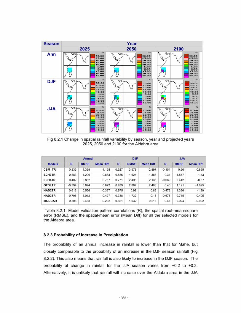
- 93 -
Year Season 2025 2050 2100
Ann
DJF
JJA
Fig 8.2.1 Change in spatial rainfall variability by season, year and projected years
2025, 2050 and 2100 for the Aldabra area
Annual DJF JJA
Models R RMSE Mean Diff R RMSE Mean Diff R RMSE Mean Diff
CSM_TR 0.335 1.399 -1.158 0.527 3.578 -2.897 -0.151 0.96 -0.895
ECH3TR 0.583 1.206 -0.853 0.886 1.624 -1.385 0.31 1.547 -1.43
ECH4TR 0.402 0.882 0.767 0.771 2.496 2.135 -0.069 0.442 -0.37
GFDLTR -0.394 0.874 0.672 0.939 2.887 2.403 0.46 1.121 -1.025
HAD2TR 0.613 0.556 -0.397 0.975 0.98 0.89 0.476 1.396 -1.29
HAD3TR -0.795 1.012 -0.427 0.338 1.732 0.15 -0.675 0.745 -0.405
MODBAR 0.505 0.468 -0.232 0.881 1.032 0.216 0.41 0.924 -0.902
Table 8.2.1: Model validation pattern correlations (R), the spatial root-mean-square error (RMSE), and the spatial-mean error (Mean Diff) for all the selected models for the Aldabra area. 8.2.3 Probability of Increase in Precipitation The probability of an annual increase in rainfall is lower than that for Mahe, but
closely comparable to the probability of an increase in the DJF season rainfall (Fig
8.2.2). This also means that rainfall is also likely to increase in the DJF season. The
probability of change in rainfall for the JJA season varies from +0.2 to +0.3.
Alternatively, it is unlikely that rainfall will increase over the Aldabra area in the JJA
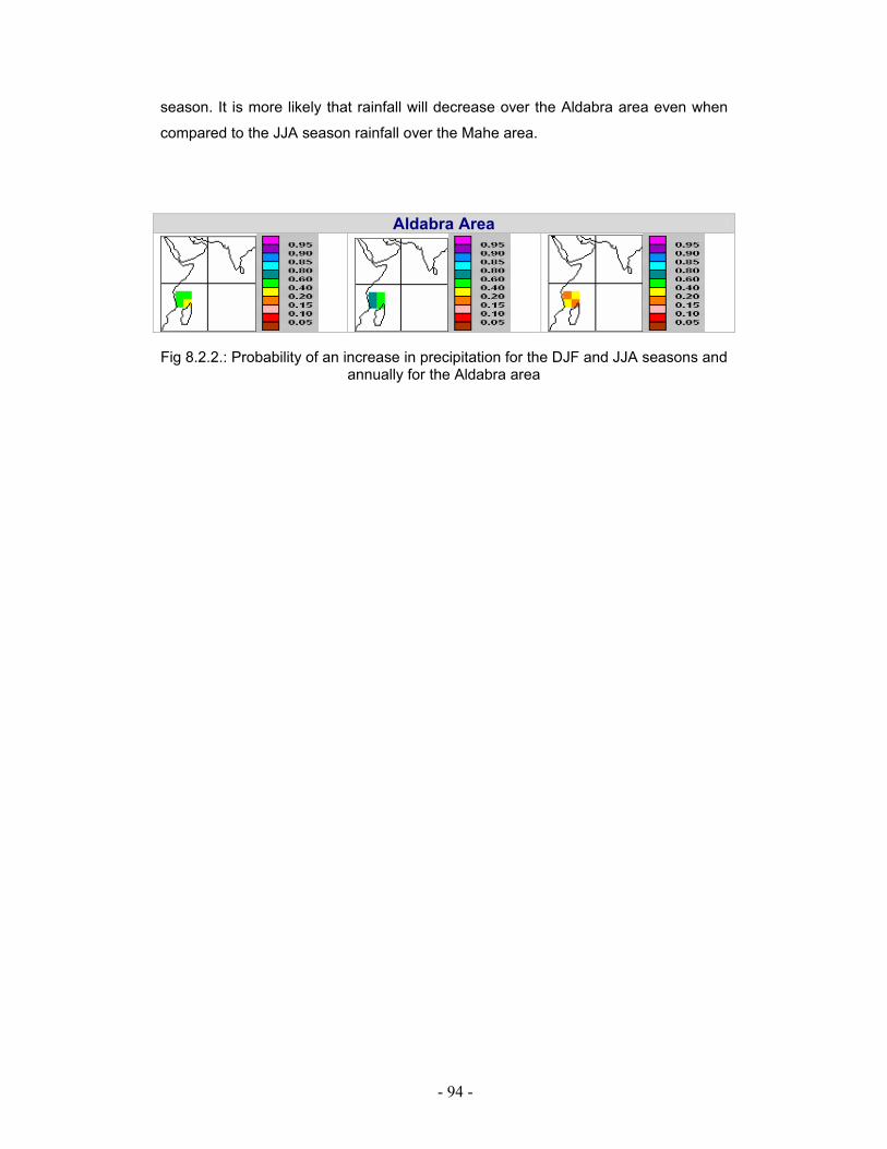
- 94 -
season. It is more likely that rainfall will decrease over the Aldabra area even when
compared to the JJA season rainfall over the Mahe area.
Aldabra Area
Fig 8.2.2.: Probability of an increase in precipitation for the DJF and JJA seasons and
annually for the Aldabra area
- 95 -
Chapter 9
Summary, Conclusion and Recommendations 9.1 Summary The MAGICC SCENGEN tool is used extensively to construct two climate scenarios
for Mahe and the Aldabra area based on the A1 high-range emission with a high
climate sensitivity and the B2 mid-range emission with a mid climate sensitivity at
seasonal and annual time scales. A range of seven General Circulation Models
(GCMs) at 5 ° (~500 km) resolution are employed to assess the regional climate
change patterns. The GCM-Guided Perturbation Method (GPM) and the Regional
Climate-Change Projection from Multi-Model Ensembles (RCPM) technique provide
an alternative assessment for comparing with the different scenario results. Scenario
uncertainties are also explored as a means of quantifying regional climate change
patterns and the choice of model selection. This will offer a range of policies and
strategies for climate change adaptation. The local parameters assessed are rainfall,
maximum and minimum temperatures, and regional sea level.
Mahe Rainfall Individual GCM output shows a maximum increase in rainfall of +5.9 % (+19 mm) for
the year 2025; +9.3 % (+25.4 mm) for the year 2050 and +12.4 % (+38.6 mm) for the
year 2100. In contrast, models shows that the JJA season will be characterized by a
deficit of -12.7 % (-9.9 mm) in rainfall for the year 2025, but surprisingly rainfall is
expected to increase in the JJA season by +22.7 % (+18.4 mm) for 2050. A decrease
of -36.3 % (-31.1 mm) is expected for the JJA season in the year 2100. It is not clear
what may cause an increase in the JJA season rainfall in the 2050s. However, it may
be linked to the upward trend in the multi-decadal 30-year cycle in rainfall variability
in the Seychelles (Chang-Seng, 2007).
Similar results are obtained using GCMs composite (average) analyses. The
composite change in rainfall for the DJF, MAM, JJA and the SON seasons for the
year 2025 is +3.7 %, +2.0 %, -3.3% and +3.8 % respectively. The year 2050
composite change in rainfall for the same respective months is +5.3%, + 4.3%,

- 96 -
+7.3 % and +2.4 %. The year 2100 composite rainfall changes are +4.9%, +10.5%, -
10.8 %, and +11.8 % for the DJF, MAM, JJA and SON seasons respectively.
The annual maximum change in rainfall is predicted by the ECH4 model with +4.9 %,
+8.5 %, +16.3 % in the years 2025, 2050 and 2100 respectively. The lowest change
in rainfall is predicted by the Had3 model with -2.4 %, -4.8 % and -8.6 % respectively
for the years 2025, 2050 and 2100. The projected change in average annual rainfall
are +1.7 % (+37.9 mm), +2.7 %( +58.2 mm), and 5.5% (+118.7 mm) respectively for
the years 2025, 2050 and 2100.
Mahe Temperature The individual- extreme GCMs scenario of seasonal temperature for the DJF season
shows a warming between +0.5 to +0.6 ° C for the year 2025; +0.9 to +1.1 ° C for
the year 2050 and +1.6 to +2.5 ° C for the year 2100. The range of temperature
warming is from +0.5 to +0.8 ° C for the year 2025, +0.8 to +1.6 ° C for the year 2050
and +1.6 to +2.9 ° C for the JJA season in the year 2100.
On the other hand, the GCMs seasonal average temperature changes for the year
2025 are +0.5 and +0.6 ° C respectively. The average temperature warming for these
respective months for the year 2050 is +1.0, +1.1 ° C and +2.0 and +2.1 ° C
respectively for the year 2100. The composite temperature pattern also shows
warming up to 2100, particularly during the MAM and JJA seasons. This implies the
future climate during the southeast monsoon will be characterized by relatively
warmer conditions.
The extreme annual warming is predicted by the ECH4 model with +0.7, +1.3, and
+2.6 ° C respectively for the years 2025, 2050 and 2100. The CSM model shows
lower temperature change of +0.5, +0.9 and +1.8 ° C respectively for the years 2025,
2050 and 2100. The annual average temperature shows warming of +0.6, +1.1 and
+2.1 ° C respectively for the above mentioned years.
Comparison between the two Climate Scenarios
In general, the comparison between the two climate scenarios shows clearly that the
A1 high-range emission with a high climate sensitivity scenario simulates extreme

- 97 -
climate changes compared to the B2 mid-range emission with mid-range climate
sensitivity.
The Aldabra Area Rainfall
The Aldabra area extreme seasonal rainfall for the DJF season shows an increase of
+7.2 % for the year 2025; +12.6 % for the year 2050 and +19.5 % for the year
2100.The GCMs projection for the JJA season shows a significant decrease in
rainfall of -17.4 % for the year 2025, -30.1 % for the year 2050 and -44.6 % for the
year 2100. On the other hand, the GCM average simulations of rainfall show a
slightly wetter-climate for the DJF season and a significantly dryer climate of up to -
21.1 % below normal for the Aldabra area rainfall by the year 2100.
Thus, a major deficit in rainfall is projected for the Aldabra area during the southeast
monsoon; however, the annul changes in rainfall for the projected years are not
significant. The same results were tested in the case of the P50 emission -business
as usual scenario. Individual GCMs show further deficit of -53.7% in the Aldabra
area rainfall during the JJA season in the year 2100. Thus, a critical climatic
threshold is identified that may threaten the sustainability of the Aldabra ecosystem.
Therefore, the Aldabra environmental eco-system is classified as highly vulnerable to
climate changes.
Aldabra Area Temperature The GCMs projected change in extreme seasonal temperature for the DJF season
shows warming ranging between +0.5 to +0.6 ° C for the year 2025, +0.8 to +1.1 ° C
for the year 2050 and +1.6 to +2.1 ° C for the year 2100. A warming between +0.5 to
+0.8 ° C is expected for the JJA season of the year 2025, +0.8 to +1.5 ° C for the year
2050 and +1.5 to +2.9 ° C for the year 2100. On the other hand, the GCMs composite
(average) shows relatively warmer temperatures during the JJA season compared to
the DJF season. The average temperature changes for the year 2025 are +0.5, and
+0.7 ° C for the DJF and JJA seasons respectively. The year 2050 temperature
changes for these respective months are +1.0 and +1.2 ° C. The individual model of
seasonal temperature change for the year 2100 is +1.9 and +2.2 ° C for the DJF and
JJA seasons respectively. The annual extreme temperature warming ranges from
+0.4 to +0.6 ° C for the year 2025; from +0.9 to +1.4 ° C for the year 2050 and from
- 98 -
+2.0 to +2.9 ° C for the year 2100. On the other hand, the GCM predicted average
temperature warming for the years 2025, 2050 and 2100 are +0.6, +1.2, and +2.6 ° C
respectively.
General Circulation Model (GCM)-Guided Perturbation Method (GPM) Overall NACR-PCM and NCAR-CSM GCM-Guided Perturbation Method (GPM)
shows significantly wetter-like climate for most of the months, especially during the
rainy season. The other models tend to be insensitive and there are large model
differences. The GCM-GPM indicates the complete absence of droughts in the future.
Most GCM-GPM temperature scenarios show that the southeast monsoon would
become warmer than the northwest monsoon (DJF) with the exception of the NACR-
CSM model. This suggests a total shift in the temperature patterns. However, the
GCM-GPM rainfall scenarios are out of phase with the thermodynamic -temperature
scenarios. Thus, only NACR-CSM results should be considered as meaningful.
Regional Climate-Change Projection from Multi-Model Ensembles (RCPM)
The DJF season precipitation rate shows a 45 to 55% chance of up to +0.8 mm per
day for the years 2025 and 2050. However, it is not very clear if the JJA season will
become dryer or wetter. The associated temperature change shows a 50%-80%
likely chance of a warming, ranging from +0.5 to +1.2 ° C and from +1.1 to +1.7 ° C
respectively.
In the case of the year 2090, RCPM results suggest close to 50 % chance of an
increase in precipitation rate of up to +1.0 mm per day for the DJF season. In
contrast, it is unlikely (15%) that precipitation rate will decrease for the same period.
There is a 55 % chance of a slight decrease in precipitation rate of -0.2 mm per day
in the JJA season in the year 2090. On an annual basis, there is a high probability of
80% for an increase in rainfall exceeding 0.5 mm per day from the years 2030 to
2100. Overall, it is likely (80%) that the climate will be wetter by the year 2100. There
is a likely chance (80%) of warming between +2.2 and +2.7 ° C in the year 2090 for
both seasons. On an annual basis there is a more likely than not chance (60 %) for a
warming between +0.5 and +1.3 ° C, +1.0 to +1.7 ° C and 2.0 to +2.7 ° C respectively
for the years 2030, 2050 and 2090.
- 99 -
Scenario Uncertainties
Climate scenario uncertainties are important for a wide range of policy and decision
making. The assessment also includes uncertainties in regional climate change
patterns and GCMs selection. There are rather large changes in variability ranging
from 25% to 32 % for the two seasons; hence models tend to agree for a wetter DJF
season and a dryer JJA season by the year 2100.
The model-to-model pattern correlations for normalized variability change fields for
the selected models show some disagreement in terms of the seasonal comparison.
ECH4D and the HAD3D tend to have the greater differences with the other models.
ECH4 model tends to predict maximum rainfall changes while HAD3D predicts
minimum change in rainfall.
Model Error ECH3 and ECH4 have the lowest model error and mean difference in simulating
current climate patterns with observed climate at an annual scale. ECH3 also turns
out to have the model with the least error in simulating present DJF season rainfall.
In contrast, MODBAR followed by the CSM, ECH4 models have the least error in
simulating current JJA seasonal rainfall.
Probability of Increase in Rainfall
It is likely (50-80 %) that the DJF season and the annual rainfall will increase and it is
unlikely to increase in the JJA season (20-40%). The probability of an increase in the
Aldabra area annual rainfall is lower than Mahe and it is more likely that the Aldabra
area rainfall will decrease compared to the Mahe area in the JJA season up to the
year 2100. Regional Sea Level Thus global sea level is expected rise from 7-8, 15-17 and 35-40 cm respectively
according to the policy best guess scenario for the years 2025, 2050 and 2100. The
HadCM2 and HadCM3 with the IS92 or P50 business as usual emission scenario
- 100 -
shows annual sea level rise ranging from +0.4 to +0.6 meter for the 2070-2100
period.
Tropical cyclone On the other hand, despite advances in computer numerical modeling of the global
climate using various scenarios of greenhouse gas emissions, making projections of
how tropical cyclones may change in frequency and intensity remain a significant
challenge. Since tropical cyclone activity is modulated by the El Niño Southern
Oscillation (ENSO) and wind shear, projections of cyclone frequency will partly
depend on the projections of future ENSOs. It is uncertain how ENSO will change in
a warmer world. Some studies have suggested that peak winds may increase by 5 to
10 % and peak rainfall rates may rise by 20 to 30 %.
9.2 Conclusion
A1 high range emission and high climate sensitivity simulates more extreme climate
changes compared to the B2 mid-range emission with mid-range climate sensitivity
(BM). The BM climate scenario shows that the mean air temperature for both Mahe
and the Aldabra area is more likely than not to warm by +3.0 ° C by the end of this
century. The relative rate of warming will occur mainly during the cooler southeast
monsoon. The warming ranges are +0.4 to +0.7; +0.9 to +1.4 and +1.8 to +2.9 ° C
respectively for the years 2025, 2050 and 2100. Consequently, the maximum
increase in seasonal rainfall for Mahe is +12.4 %( +38.6 mm) in the DJF season
while a decrease of -36.3% (-31.1 mm) is expected during the southeast monsoon of
the year 2100. The range of percentage change in annual rainfall is -2.4 to +5.0 %; -
4.8 to +8.5 %; -8.6 to +16.3 % respectively for the years 2025, 2050 and 2100. Thus,
the rainy season is more likely than not to be wetter, while the dry season is more
likely than not to be dryer with the exception of the JJS season of the year 2050. It is
suggested that the projected upward trend in the multi-decadal 30 year-cycle in
rainfall variability (Chang-Seng, 2007) could possibly balance the expected deficit
during the JJA season of the year 2050 forced by anthropogenic climate changes.
Scenario uncertainties methods such as change in model variability and probability of
an increase in precipitation analyses support quantitatively that the DJF season will
likely be wetter while the JJA season is unlikely to be wetter and the annual rainfall
will likely be higher than the 1972-1990 base periods.

- 101 -
The Regional Climate-Change Projection from Multi-Model Ensembles RCPM shows
seasonal precipitation rates are more likely than not (45-55%) to increase in the rainy
season of up to +1.0 mm per day by the year 2100.On an annual basis it is likely
(80%) that rainfall rate will be greater and equal to +0.5 mm per day.
A critical rainfall threshold of a deficit of -44% (B2 mid-range emission and mid range
climate sensitivity) and -53.7 % (P50 business as usual emission) in the JJA season
rainfall is identified for the Aldabra area by the year 2100. However, the annual
rainfall is unlikely to change significantly. The major deficit in the JJA season by the
turn of this century threatens the sustainability of the Aldabra Atoll. Thus, the Aldabra
Atoll, one of the world’s greatest surviving natural wonders which has remained fairly
isolated and preserved (Attenborough, 1995) is now potentially most vulnerable to
anthropogenic climate changes in the Seychelles.
The climate can be characterised by more than likely than not with more extreme dry,
wet, and hot episodes.The increase in precipitation is through the thermodynamic
warming and the potential increase in atmospheric water vapour (FAR, 2007). The
expected dryness particularly in the JJA season of the year 2100 is likely to be linked
to the expected extreme warming in the northern hemisphere which would drive a
stronger southeast monsoon, thus inhibiting cloud and rainfall formation in the
southwest Indian Ocean.
Model evaluation shows that ECH3 and ECH4 general circulation models have the
least error in simulating current climate pattern to observed climate. However,
MODBAR model has the least error in simulating the JJA season climate. Overall,
model performance is dependent on the choice of time scale selected.
Global sea level is expected to rise from +7-8, +15-17 and +35-40 cm according to
the policy best guess scenario by the years 2025, 2050 and 2100 respectively.
Regional sea level in the southwest Indian Ocean is expected to rise between +40 to
+60 cm according to the UK Meteorological Office model. On the other hand, tropical
cyclone scenario remains a major challenge, but recent modeling studies in the US,
have suggested that peak winds may increase by 5 to 10 % and peak rainfall rates
may rise by 20 to 30 %.

- 102 -
9.3 Recommendations It is recommended that future climate change scenario assessment should consider
higher resolution model to provide more skillful island-type of climate scenarios. It is
also envisaged that climate downscaling can be applied to achieve far better results
at a national level. Future work should also focus on verifying the ‘critical’ climate
changes identified here in this assessment.
A detailed climate change–ecological-environment impact assessment should follow
through in the case of the Aldabra area for possible mitigation and adaptation of the
impacts.
- 103 -
Reference
Chang-Seng, S. D., 2007: Climate Variability and Climate Change Assessment for the Seychelles, Second National Communication (SNC), Under the United Nations Framework Convention on Climate Change (UNFCCC). Chang-Seng, S. D., 2005: Marine Weather Systems, Tropical Cyclone Prediction and Impacts in the Southwest Indian Ocean, MSc. Thesis, Department of Geography and Environmental Studies, University of Zululand. Chang-Seng, S. D., 2002: El Nino and Indian Ocean Dipole Mode and its Impact on Sea Level and Rainfall in the Seychelles, Seychelles National Meteorological Services. Climate Change, 2007: The Physical Science Base, Summary for Policy Makers. Contribution of Working Group 1 to the Fourth Assessment Report (FAR) of the IPCC, 5th February 2007. Gray, W., 1984a: Atlantic Seasonal Hurricane Frequency. Part I: El Nino and 30 mb Quasi-Biennial Oscillation Influences. Mon. Wea. Rev., 112: 1649-1668. Gray, W., 1984b; Atlantic Seasonal Hurricane Frequency. Part II: Forecasting its Variability. Mon. Wea. Rev., 112: 1669-1683. Hoareau, K., 1999: La Fréquence des Cyclones Tropicaux Intenses dans le Sud-Ouest de L'ocean Indien (1970-1999). Publications de l'Association Internationale de Climatologie, 12: 405-413. Hulme. M., Wigley et al, 2000: Using a Climate Scenario Generator for Vulnerability and Adaptation Assessments: Magicc Scengen V2.4 workbook Jury, M. R., and Parker B. A., 1999: Synoptic Environment of Composite Tropical Cyclones in the South-West Indian Ocean. S. A. J. Marine Sci., 21: 99-115. Lajoie, F. R., 2004: WMO/CLIVAR ETCCDMI African Workshop on Extremes, Report for Seychelles Leuliette, E. W., Nerem. R. S., and Mitchum, G., 2004: Results of TOPEX/Poseidon and Jason Calibration to Construct a Continuous Record of Mean Sea Level, Mar.Geod, In Press. Marguerite., T. M., 2001: Solar activity long term influence on Seychelles rainfall, Meteorological Services, Seychelles

- 104 -