Embed Size (px)
Citation preview
SFU CMPT-307 2008-2 1 Lecture: Week 4
SFU CMPT-307 2008-2 Lecture: Week 4
Jan Manuch
E-mail: [email protected]
Lecture on May 27, 2008, 5.30pm-8.20pm
Last modified: Tuesday 27th May, 2008, 11:38 2008 Jan Manuch

SFU CMPT-307 2008-2 2 Lecture: Week 4
Performance of Quicksort
the running time depends on how balanced or unbalanced the partitions
are;
and this depends on the choice of pivots
intuitively, if partitions arebalanced,then as in case of Mergesort,
the running time isO(n log n);if they are veryunbalanced,it can run as slow as Selection-Sort
and the running time is(n2)
Last modified: Tuesday 27th May, 2008, 11:38 2008 Jan Manuch
SFU CMPT-307 2008-2 3 Lecture: Week 4
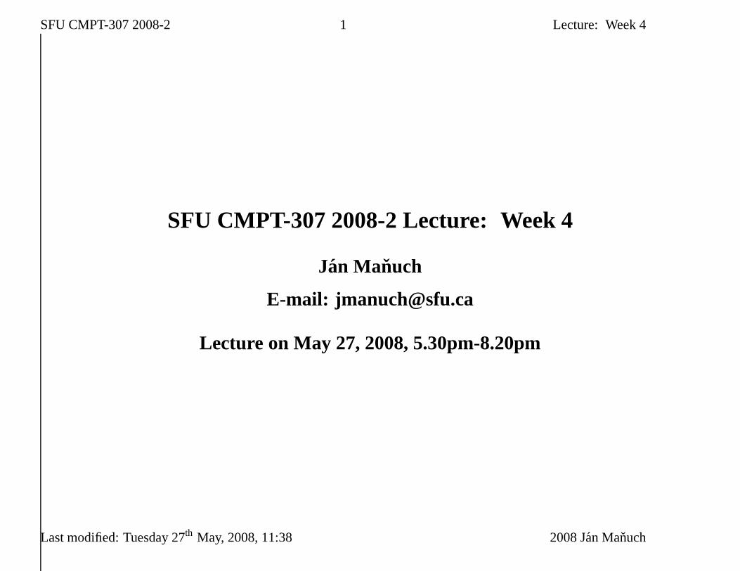
The worst case partitioning
occurs when one partition hasn� 1 elements and the other is empty (0
elements)
assume that such a partitioning happens in each recursion call
recursive call to empty array just returns the control back,which takesT (0) = O(1) time, so we get the recurrence for the running time:T (n) = T (n� 1) + T (0) + �(n)= T (n� 1) + �(n)which is the sum of arithmetic series=)T (n) = �(n2)
Note: this bad partitioning can really happen (see assignment), and so we
get the lower bound for the worst running time(n2)on the other hand we will prove the same upper bound
Last modified: Tuesday 27th May, 2008, 11:38 2008 Jan Manuch
SFU CMPT-307 2008-2 4 Lecture: Week 4
Assignment Problem 4.1.(deadline: June 3, 5:30pm)
Show that the running time of theQuicksort presented at the lecture is�(n2) when the elements of the arrayA are distinct and sorted
(a) in increasing order;
(b) in decreasing order.
Last modified: Tuesday 27th May, 2008, 11:38 2008 Jan Manuch
SFU CMPT-307 2008-2 5 Lecture: Week 4
Worst-case performance
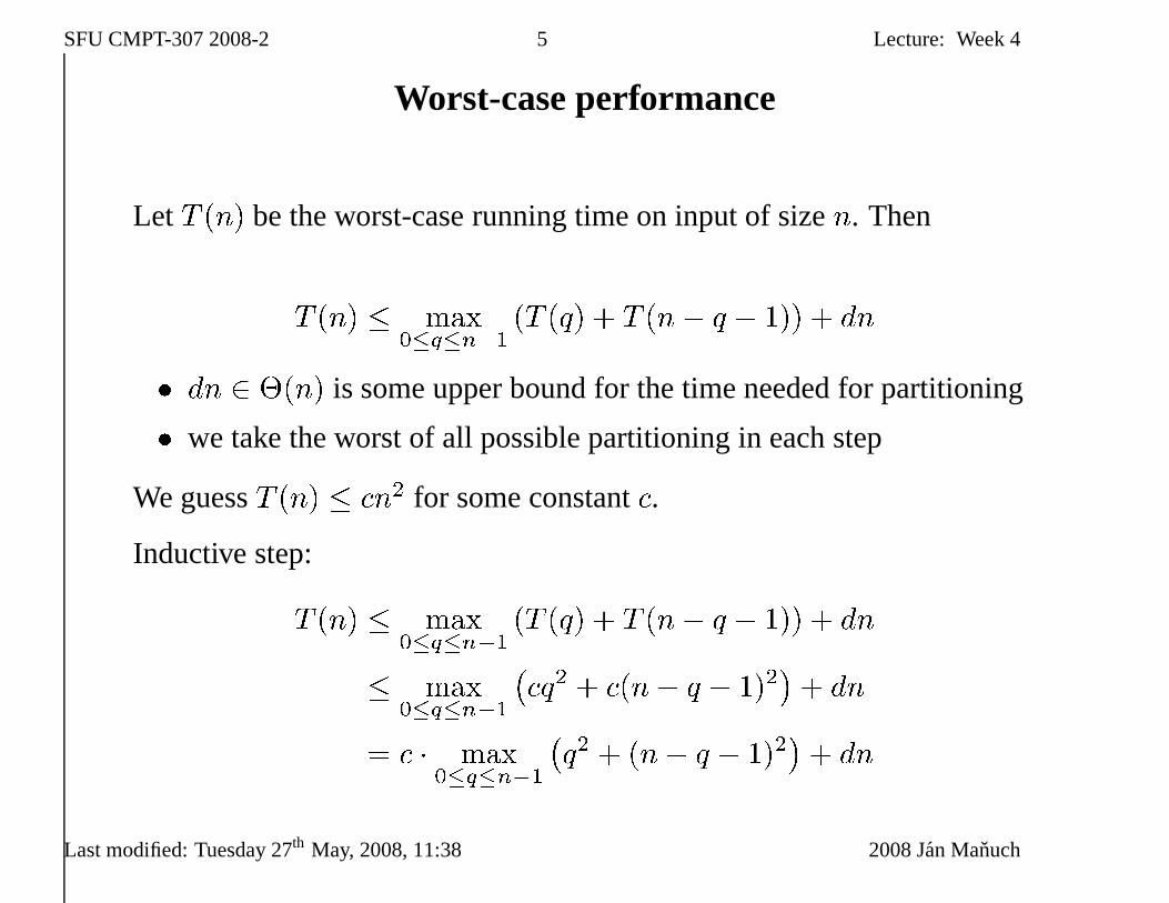
Let T (n) be the worst-case running time on input of sizen. Then
T (n) � max0�q�n�1 (T (q) + T (n� q � 1)) + dn� dn 2 �(n) is some upper bound for the time needed for partitioning� we take the worst of all possible partitioning in each step
We guessT (n) � n2 for some constant .Inductive step:T (n) � max0�q�n�1 (T (q) + T (n� q � 1)) + dn� max0�q�n�1 � q2 + (n� q � 1)2�+ dn= � max0�q�n�1 �q2 + (n� q � 1)2�+ dn
Last modified: Tuesday 27th May, 2008, 11:38 2008 Jan Manuch
SFU CMPT-307 2008-2 6 Lecture: Week 4
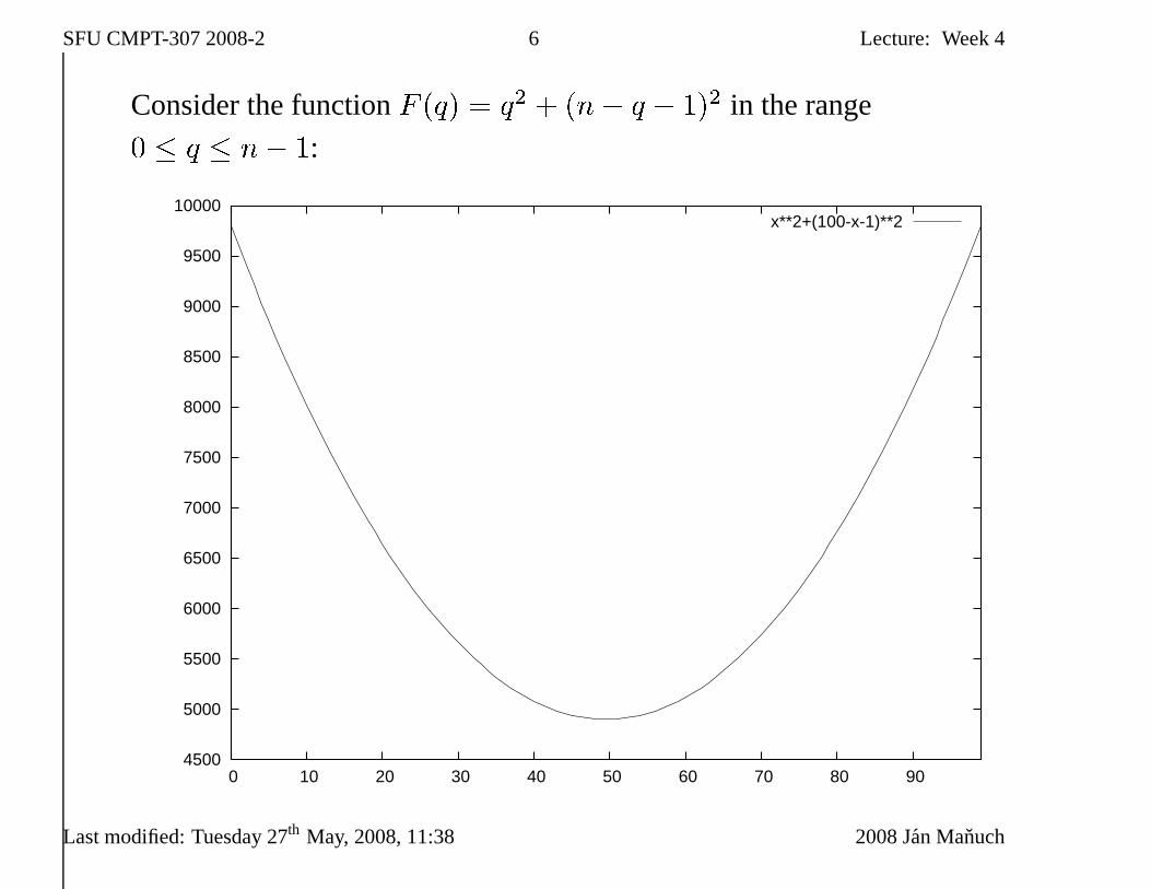
Consider the functionF (q) = q2 + (n� q � 1)2 in the range0 � q � n� 1:
4500
5000
5500
6000
6500
7000
7500
8000
8500
9000
9500
10000
0 10 20 30 40 50 60 70 80 90
x**2+(100-x-1)**2
Last modified: Tuesday 27th May, 2008, 11:38 2008 Jan Manuch
SFU CMPT-307 2008-2 7 Lecture: Week 4
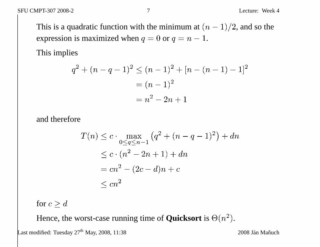
This is a quadratic function with the minimum at(n� 1)=2, and so theexpression is maximized whenq = 0 or q = n� 1.
This impliesq2 + (n� q � 1)2 � (n� 1)2 + [n� (n� 1)� 1℄2= (n� 1)2= n2 � 2n+ 1and thereforeT (n) � � max0�q�n�1 �q2 + (n� q � 1)2�+ dn� � (n2 � 2n+ 1) + dn= n2 � (2 � d)n+ � n2
for � d
Hence, the worst-case running time ofQuicksort is�(n2).Last modified: Tuesday 27th May, 2008, 11:38 2008 Jan Manuch

SFU CMPT-307 2008-2 8 Lecture: Week 4
The best case partitioning
occurs when partitioning is even:
one partition has sizebn=2 and the otherdn=2e � 1
(that is for oddn, both have the same size, and for evenn, they differ by1)
we get the recurrence:T (n) = 2T (n=2) + �(n)which has the solutionT (n) = �(n log n)
Last modified: Tuesday 27th May, 2008, 11:38 2008 Jan Manuch
SFU CMPT-307 2008-2 9 Lecture: Week 4
Assignment Problem 4.2.(deadline: June 3, 5:30pm)
Show that the best-case running time ofQuicksort is(n log n), i.e.,
show that the recurrenceT (n) � min0�q�n�1 (T (q) + T (n� q � 1)) + dn
is in(n log n).Hint: You can use the fact that the functionf(x) = x log x+ (n� 1� x) log(n� 1� x) achieves its global
minimum at pointx = (n� 1)=2.
Last modified: Tuesday 27th May, 2008, 11:38 2008 Jan Manuch

SFU CMPT-307 2008-2 10 Lecture: Week 4
The average case partitioning (intuition)
assume that in every recursive step one partition has sizen=10 and the
other9n=10 (which seems as a quite unbalanced partitioning)
then we get the recurrence:T (n) = T (9n=10) + T (n=10) + �(n)building the recursion tree shows that we are still inO(n log n)
In fact the same is true for any constant factor partition!
Last modified: Tuesday 27th May, 2008, 11:38 2008 Jan Manuch
SFU CMPT-307 2008-2 11 Lecture: Week 4
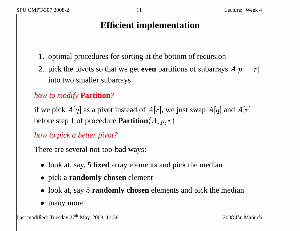
Efficient implementation
1. optimal procedures for sorting at the bottom of recursion
2. pick the pivots so that we getevenpartitions of subarraysA[p : : : r℄
into two smaller subarrays
how to modify Partition ?
if we pickA[q℄ as a pivot instead ofA[r℄, we just swapA[q℄ andA[r℄
before step 1 of procedurePartition (A; p; r)how to pick a better pivot?
There are several not-too-bad ways:� look at, say,5 fixed array elements and pick the median� pick arandomly chosenelement� look at, say5 randomly chosenelements and pick the median� many more
Last modified: Tuesday 27th May, 2008, 11:38 2008 Jan Manuch

SFU CMPT-307 2008-2 12 Lecture: Week 4
in practice, the randomized variant usually works the best
Why randomized strategy?
some of inputs (for example, if the input is sorted or almost sorted) have abad performance
in practical applications it often happens that the inputs are notcompletely random, so even if our algorithm performs good inaverage,some application might prefer the inputs with the worst-case performanceExample.� transactions on an account are usually kept in order of theirtimes� people usually write checks in order by check number, but they are
cashed with some delays� many people want the checks listed in order by check number, hence
we have to convert time-of-transaction ordering to check-number or-
dering� this is sorting of nearly sorted input, which performs very badly in
Quicksort we have considered
Last modified: Tuesday 27th May, 2008, 11:38 2008 Jan Manuch
SFU CMPT-307 2008-2 13 Lecture: Week 4
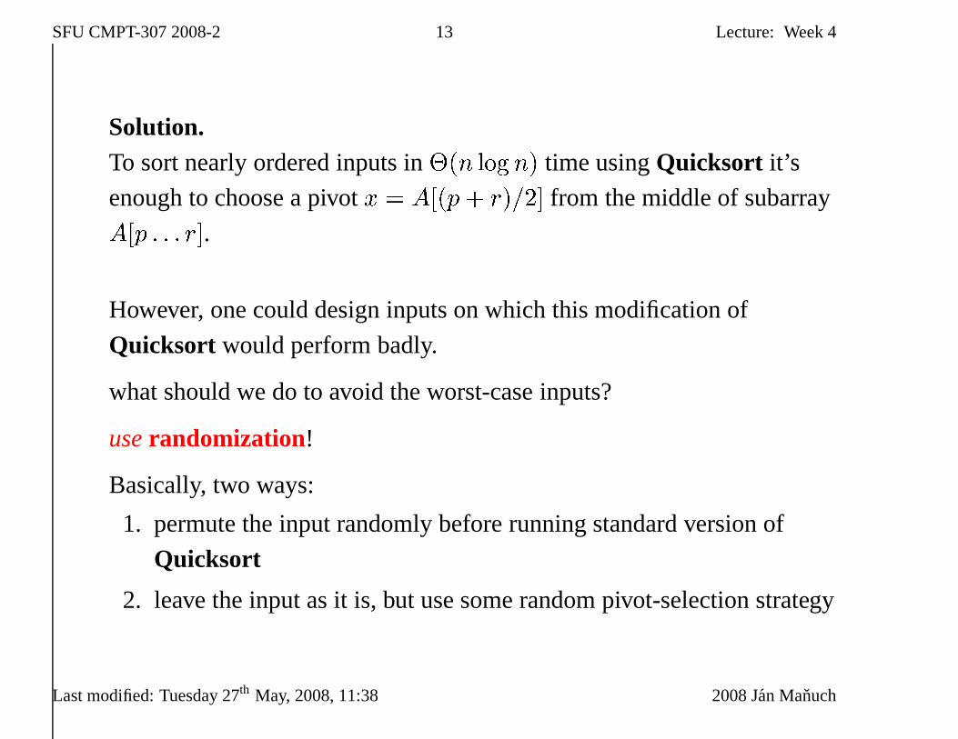
Solution.To sort nearly ordered inputs in�(n log n) time usingQuicksort it’s
enough to choose a pivotx = A[(p+ r)=2℄ from the middle of subarrayA[p : : : r℄.However, one could design inputs on which this modification of
Quicksort would perform badly.
what should we do to avoid the worst-case inputs?
use randomization!
Basically, two ways:
1. permute the input randomly before running standard version of
Quicksort
2. leave the input as it is, but use some random pivot-selection strategy
Last modified: Tuesday 27th May, 2008, 11:38 2008 Jan Manuch
SFU CMPT-307 2008-2 14 Lecture: Week 4
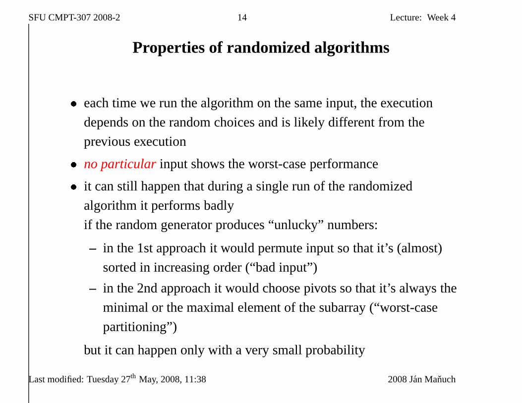
Properties of randomized algorithms� each time we run the algorithm on the same input, the execution
depends on the random choices and is likely different from the
previous execution� no particular input shows the worst-case performance� it can still happen that during a single run of the randomized
algorithm it performs badly
if the random generator produces “unlucky” numbers:
– in the 1st approach it would permute input so that it’s (almost)
sorted in increasing order (“bad input”)
– in the 2nd approach it would choose pivots so that it’s alwaysthe
minimal or the maximal element of the subarray (“worst-case
partitioning”)
but it can happen only with a very small probability
Last modified: Tuesday 27th May, 2008, 11:38 2008 Jan Manuch
SFU CMPT-307 2008-2 15 Lecture: Week 4
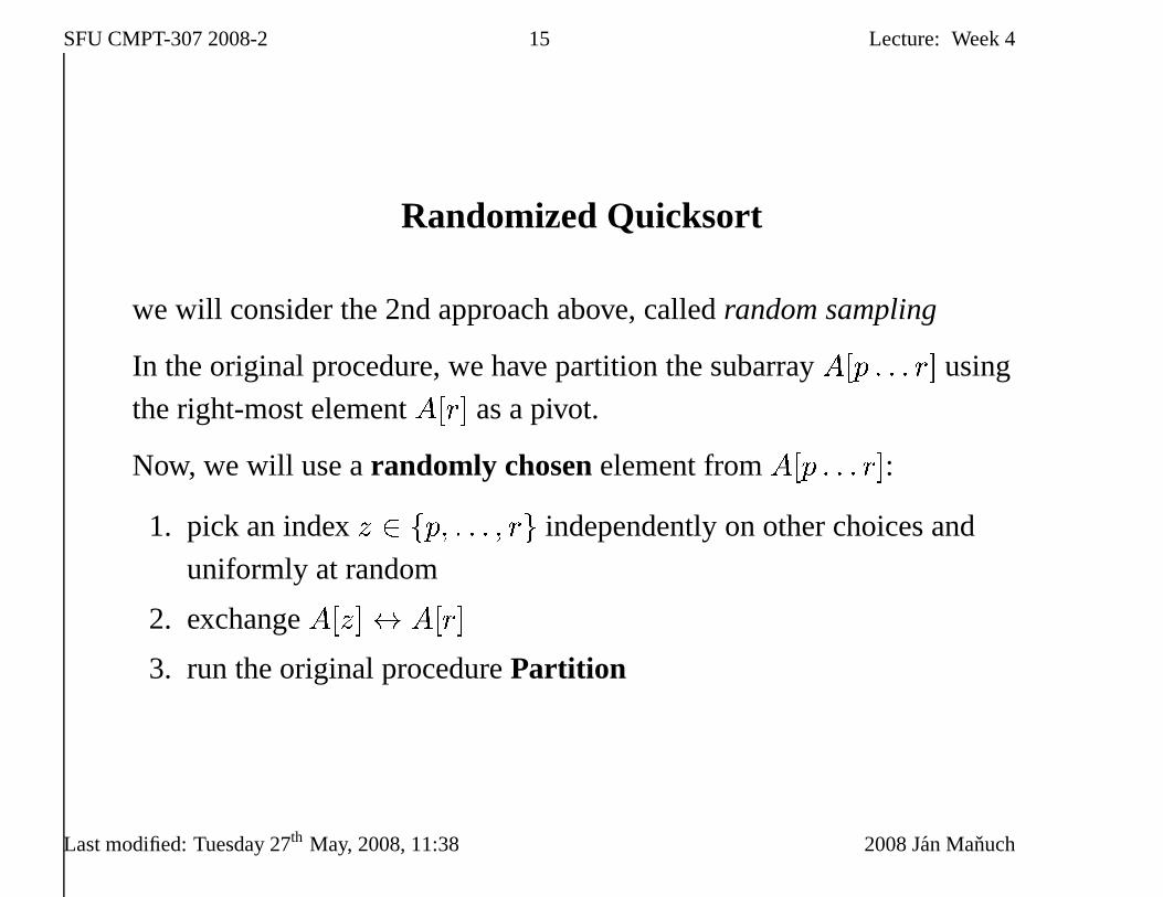
Randomized Quicksort
we will consider the 2nd approach above, calledrandom sampling
In the original procedure, we have partition the subarrayA[p : : : r℄ using
the right-most elementA[r℄ as a pivot.
Now, we will use arandomly chosenelement fromA[p : : : r℄:1. pick an indexz 2 fp; : : : ; rg independently on other choices and
uniformly at random
2. exchangeA[z℄$ A[r℄
3. run the original procedurePartition
Last modified: Tuesday 27th May, 2008, 11:38 2008 Jan Manuch

SFU CMPT-307 2008-2 16 Lecture: Week 4
Randomized-Partition(A; p; r)
1: z Random(p; r)2: exchangeA[z℄$ A[r℄3: return Partition(A; p; r)
Note: procedureRandom(a; b) returns an integer from the setfa; a+ 1; : : : ; b� 1; bg each with the same probability1=(b� a+ 1)
(“uniform distribution”)
Randomized-Quicksort(A; p; r)1: if p < r then2: q Randomized-Partition(A; p; r)3: Randomized-Quicksort(A; p; q � 1)4: Randomized-Quicksort(A; q + 1; r)5: end if
Before we can start analyzing performance ofRandomized-Quicksortwe need to recall basics ofprobability theory
Last modified: Tuesday 27th May, 2008, 11:38 2008 Jan Manuch

SFU CMPT-307 2008-2 17 Lecture: Week 4
Probability
Defined in terms of aprobability spaceor sample spaceS (or ), asetwhose elementss 2 S (or ! 2 ) are calledelementary events.
you can view elementary events as possible outcomes of an experiment.
Examples:� flip a coin:S = fhead; tailg� roll a die:S = f1; 2; 3; 4; 5; 6g� pick a random pivot inA[p : : : ; r℄:S = fp; p+ 1; : : : ; rg – indexes of the pivot
Here, we are talking only aboutfinite discrete probability spaces.
Last modified: Tuesday 27th May, 2008, 11:38 2008 Jan Manuch
SFU CMPT-307 2008-2 18 Lecture: Week 4
An event is a subset of the probability space
Examples:� roll a die;A = f2; 4; 6g � f1; 2; 3; 4; 5; 6g is the event of having an
even outcome� flip two distinguishable coins:S = fHH;HT; TH; TTg, andA = fTT;HHg � S is the event of
having the same outcome with both coins
We sayS (the entire sample space) is acertain event, and; is theemptyor null event
We say eventsA andB aremutually exclusive if A \B = ;Last modified: Tuesday 27th May, 2008, 11:38 2008 Jan Manuch
SFU CMPT-307 2008-2 19 Lecture: Week 4
Axioms
A probability distribution P () onS is mapping from events ofS to real
numbers in interval[0; 1℄ such that
1. P (A) � 0 for all A � S2. P (S) = 1 (normalization)
3. P (A) + P (B) = P (A [B) for any twomutually exclusiveeventsA andB, i.e.,A \B = ;.Generalization: for any finite sequence of pairwise mutually
exclusive eventsA1; A2; : : :P [i Ai! =Xi P (Ai)
P (A) is calledprobability of eventA
Last modified: Tuesday 27th May, 2008, 11:38 2008 Jan Manuch
SFU CMPT-307 2008-2 20 Lecture: Week 4
Properties of probability that that follows from axioms:
1. P (;) = 02. If A � B thenP (A) � P (B)
3. With �A = S �A, we haveP ( �A) = P (S)� P (A) = 1� P (A)
4. For anyA andB (not necessarily mutually exclusive),P (A [B) = P (A) + P (B)� P (A \B)� P (A) + P (B)Considering discrete sample spaces, we have for any eventAP (A) =Xs2AP (s)If S is finite, andP (s 2 S) = 1=jSj, then we haveuniform probabilitydistribution onS (that’s what’s usually referred to as “picking an
element ofS at random”)
Last modified: Tuesday 27th May, 2008, 11:38 2008 Jan Manuch

SFU CMPT-307 2008-2 21 Lecture: Week 4
Conditional probabilities
when you already have partial knowledge
Example: a friend rolls two fair dice (prob. space isf(x; y) : x; y 2 f1; : : : ; 6gg) and tells you that one of them shows a6.What’s the probability for a(6; 6) outcome?
61 5 52 = 2562 = 36 36� 25 = 116 1=11A B
P (AjB) = P (A \B)P (B)P (B) 6= 0
Last modified: Tuesday 27th May, 2008, 11:38 2008 Jan Manuch
SFU CMPT-307 2008-2 21 Lecture: Week 4
Conditional probabilities
when you already have partial knowledge
Example: a friend rolls two fair dice (prob. space isf(x; y) : x; y 2 f1; : : : ; 6gg) and tells you that one of them shows a6.What’s the probability for a(6; 6) outcome?
The information eliminates outcomes without any6, i.e., all combinationsof 1 through5. There are52 = 25 of them. The original prob. space hassize62 = 36, thus we are left with36� 25 = 11 outcomes where at leastone6 is involved.
These are equally likely, thus the sought probability must be1=11.
Theconditional probability of an eventA given that another eventB
occurs is P (AjB) = P (A \B)P (B)givenP (B) 6= 0
Last modified: Tuesday 27th May, 2008, 11:38 2008 Jan Manuch

SFU CMPT-307 2008-2 22 Lecture: Week 4
S
A B
In the example: A = f(6; 6)gB = f(6; x) : x 2 f1; : : : ; 6gg [f(x; 6) : x 2 f1; : : : ; 6ggwith jBj = 11 (the(6; 6) is in both parts) and thusP (A \B) = P (f(6; 6)g) = 1=36 andP (AjB) = P (A \B)P (B) = 1=3611=36 = 111
Last modified: Tuesday 27th May, 2008, 11:38 2008 Jan Manuch

SFU CMPT-307 2008-2 23 Lecture: Week 4
Assignment Problem 4.3.(deadline: June 3, 5:30pm)
Show by mathematical induction that for anyn and eventsA1; A2; : : : ; An we have the equality:P (A1 \A2 \ � � � \An) =P (A1) � P (A2jA1) � P (A3jA2 \A1) � � �P (AnjAn�1 \ � � � \A2 \A1)Last modified: Tuesday 27th May, 2008, 11:38 2008 Jan Manuch
SFU CMPT-307 2008-2 24 Lecture: Week 4
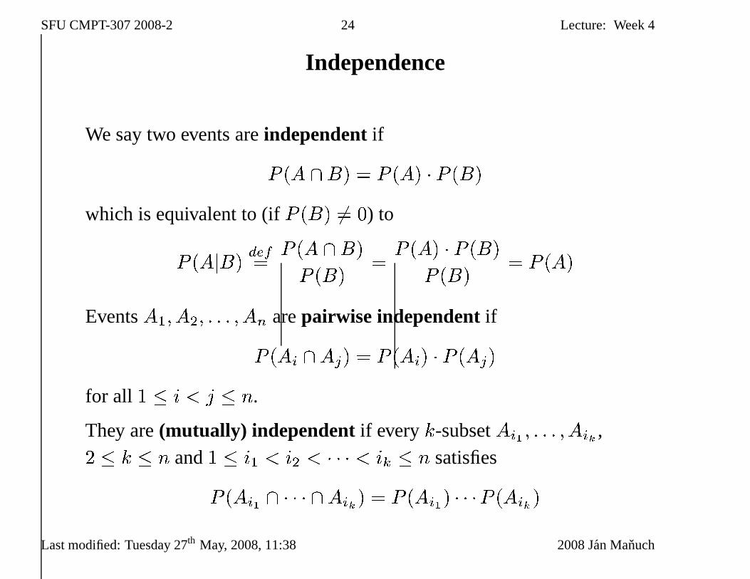
Independence
We say two events areindependentifP (A \B) = P (A) � P (B)
which is equivalent to (ifP (B) 6= 0) toP (AjB) def= P (A \B)P (B) = P (A) � P (B)P (B) = P (A)
EventsA1; A2; : : : ; An arepairwise independentifP (Ai \Aj) = P (Ai) � P (Aj)for all 1 � i < j � n.
They are(mutually) independent if everyk-subsetAi1 ; : : : ; Aik ,2 � k � n and1 � i1 < i2 < � � � < ik � n satisfiesP (Ai1 \ � � � \Aik) = P (Ai1) � � �P (Aik)Last modified: Tuesday 27th May, 2008, 11:38 2008 Jan Manuch

SFU CMPT-307 2008-2 25 Lecture: Week 4
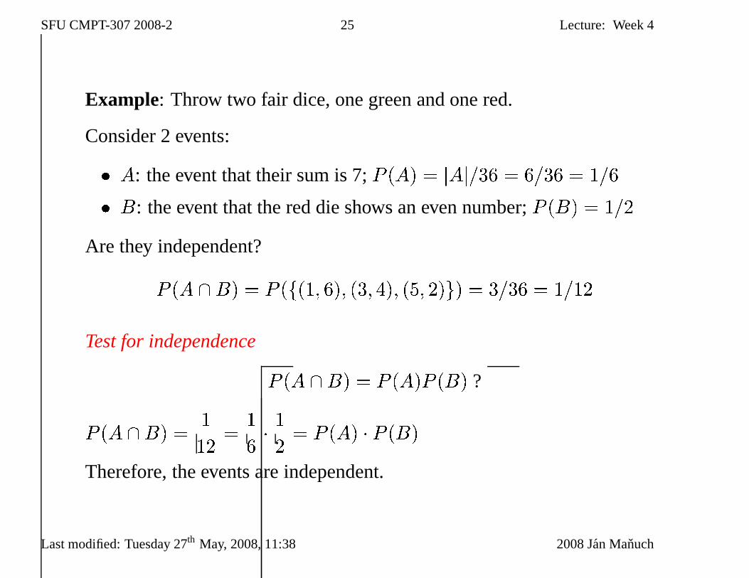
Example: Throw two fair dice, one green and one red.
Consider 2 events:� A: the event that their sum is 7;P (A) = jAj=36 = 6=36 = 1=6� B: the event that the red die shows an even number;P (B) = 1=2
Are they independent?
P (A \B) = P (f(1; 6); (3; 4); (5; 2)g) = 3=36 = 1=12
P (A \B) = P (A)P (B)P (A \B) = 112 = 16 � 12 = P (A) � P (B)
Last modified: Tuesday 27th May, 2008, 11:38 2008 Jan Manuch
SFU CMPT-307 2008-2 25 Lecture: Week 4
Example: Throw two fair dice, one green and one red.
Consider 2 events:� A: the event that their sum is 7;P (A) = jAj=36 = 6=36 = 1=6� B: the event that the red die shows an even number;P (B) = 1=2
Are they independent?P (A \B) = P (f(1; 6); (3; 4); (5; 2)g) = 3=36 = 1=12
Test for independence P (A \B) = P (A)P (B) ?P (A \B) = 112 = 16 � 12 = P (A) � P (B)Therefore, the events are independent.
Last modified: Tuesday 27th May, 2008, 11:38 2008 Jan Manuch
SFU CMPT-307 2008-2 26 Lecture: Week 4
Assignment Problem 4.4.(deadline: June 3, 5:30pm)
Consider a probability spaceS = f1; 2; : : : ; 8g (outcome of a throw of
8-sided die). Find and example of three eventsA;B;C of S such thatA;B;C are pairwise independent, but eventsA andB \ C are not (i.e.P (A) � P (B \ C) 6= P (A \B \ C)).
Last modified: Tuesday 27th May, 2008, 11:38 2008 Jan Manuch
SFU CMPT-307 2008-2 27 Lecture: Week 4
Random variables
A random variable X is a function from a probability spaceS to the set
of real numbers, i.e., it assigns some value to elementary events
Event “X = x” is defined to befs 2 S : X(s) = xg
Example: roll three dice� S = fs = (s1; s2; s3) j s1; s2; s3 2 f1; 2; : : : ; 6ggjSj = 63 = 216 possible outcomes� Uniform distribution: each element has probability1=jSj = 1=216� Let random variableX be the sum of dice, i.e.,X(s) = X(s1; s2; s3) = s1 + s2 + s3Last modified: Tuesday 27th May, 2008, 11:38 2008 Jan Manuch
SFU CMPT-307 2008-2 28 Lecture: Week 4
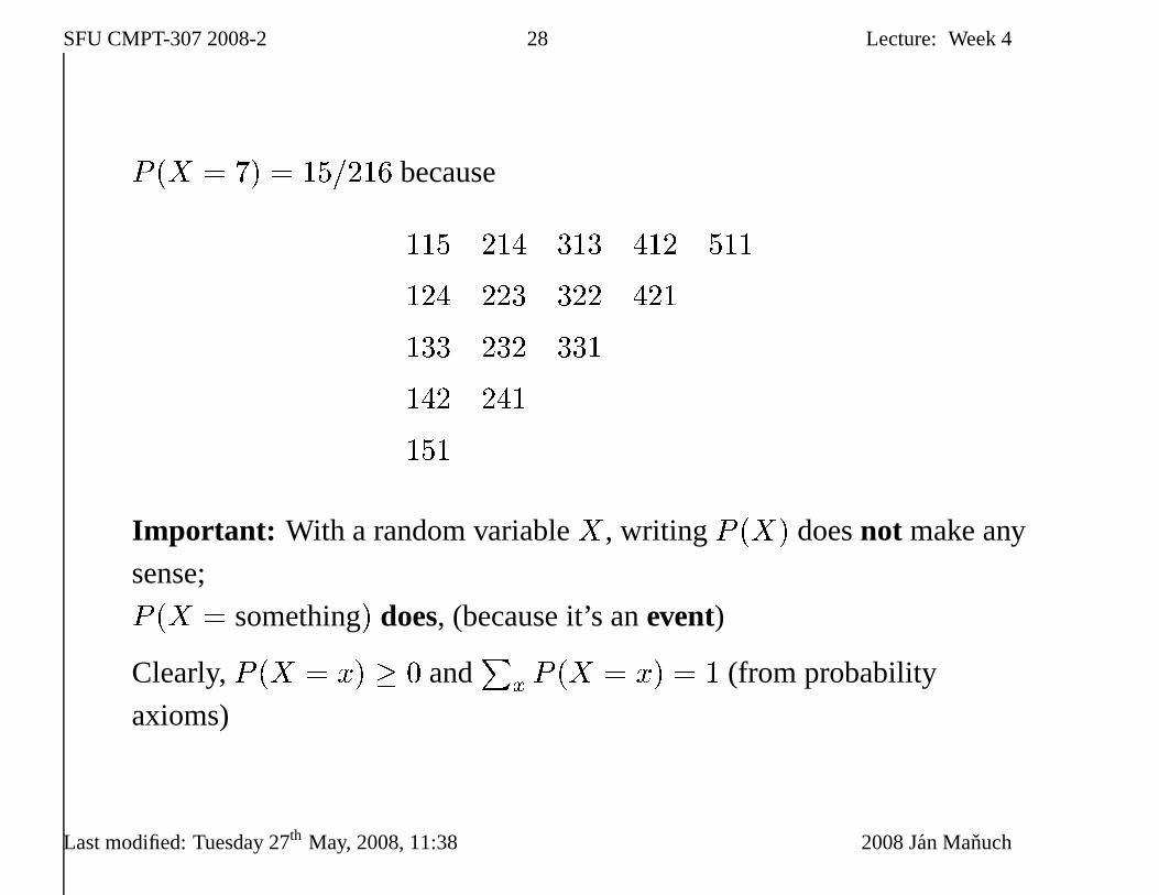
P (X = 7) = 15=216 because115 214 313 412 511124 223 322 421133 232 331142 241151Important: With a random variableX, writing P (X) doesnot make any
sense;P (X = something) does, (because it’s anevent)
Clearly,P (X = x) � 0 and
Px P (X = x) = 1 (from probability
axioms)
Last modified: Tuesday 27th May, 2008, 11:38 2008 Jan Manuch
SFU CMPT-307 2008-2 29 Lecture: Week 4
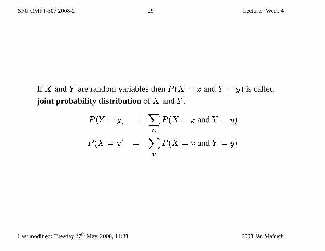
If X andY are random variables thenP (X = x andY = y) is called
joint probability distribution of X andY .P (Y = y) = Xx P (X = x andY = y)P (X = x) = Xy P (X = x andY = y)Last modified: Tuesday 27th May, 2008, 11:38 2008 Jan Manuch
SFU CMPT-307 2008-2 30 Lecture: Week 4
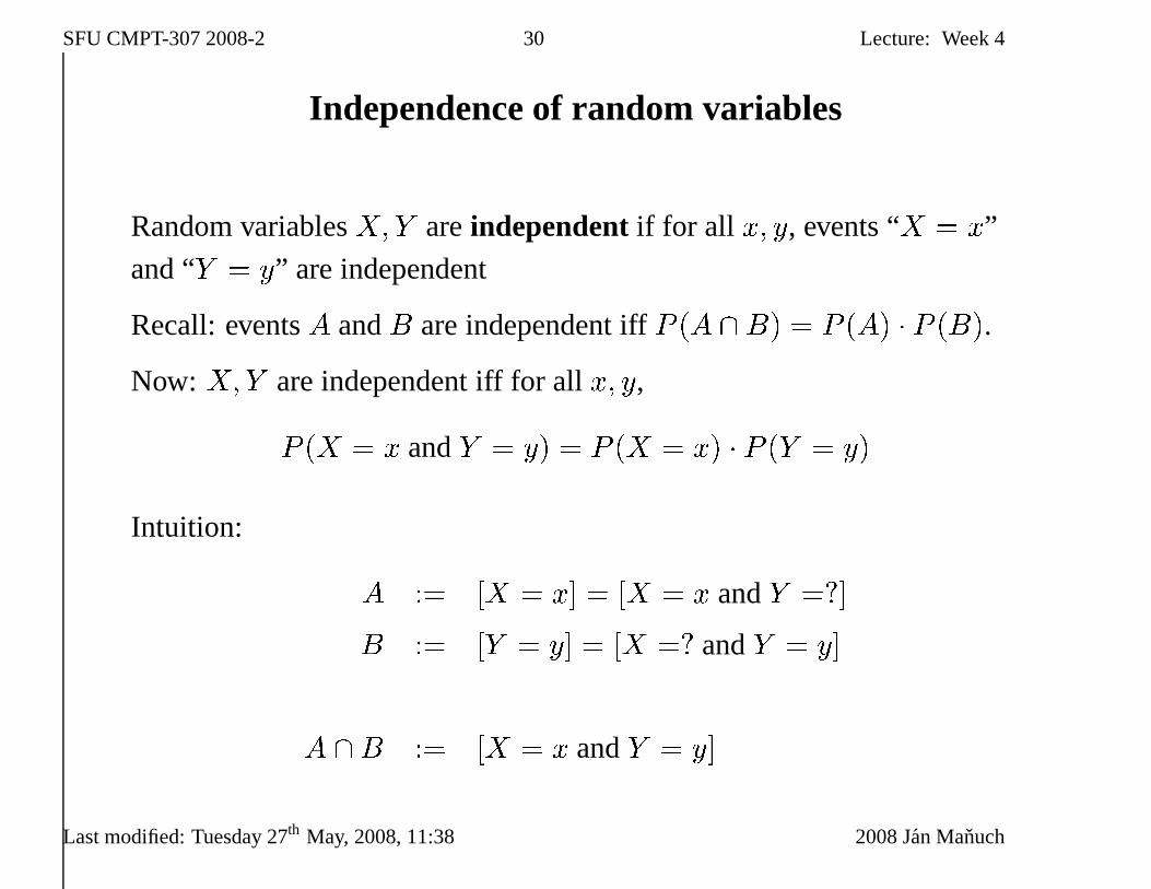
Independence of random variables
Random variablesX;Y areindependentif for all x; y, events “X = x”
and “Y = y” are independent
Recall: eventsA andB are independent iffP (A \B) = P (A) � P (B).Now: X;Y are independent iff for allx; y,P (X = x andY = y) = P (X = x) � P (Y = y)
Intuition: A := [X = x℄ = [X = x andY =?℄B := [Y = y℄ = [X =? andY = y℄
A \B := [X = x andY = y℄Last modified: Tuesday 27th May, 2008, 11:38 2008 Jan Manuch
SFU CMPT-307 2008-2 31 Lecture: Week 4
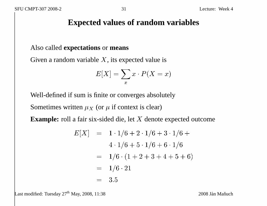
Expected values of random variables
Also calledexpectationsor means
Given a random variableX, its expected value isE[X℄ =Xx x � P (X = x)
Well-defined if sum is finite or converges absolutely
Sometimes written�X (or � if context is clear)
Example: roll a fair six-sided die, letX denote expected outcomeE[X℄ = 1 � 1=6 + 2 � 1=6 + 3 � 1=6 +4 � 1=6 + 5 � 1=6 + 6 � 1=6= 1=6 � (1 + 2 + 3 + 4 + 5 + 6)= 1=6 � 21= 3:5
Last modified: Tuesday 27th May, 2008, 11:38 2008 Jan Manuch
SFU CMPT-307 2008-2 32 Lecture: Week 4
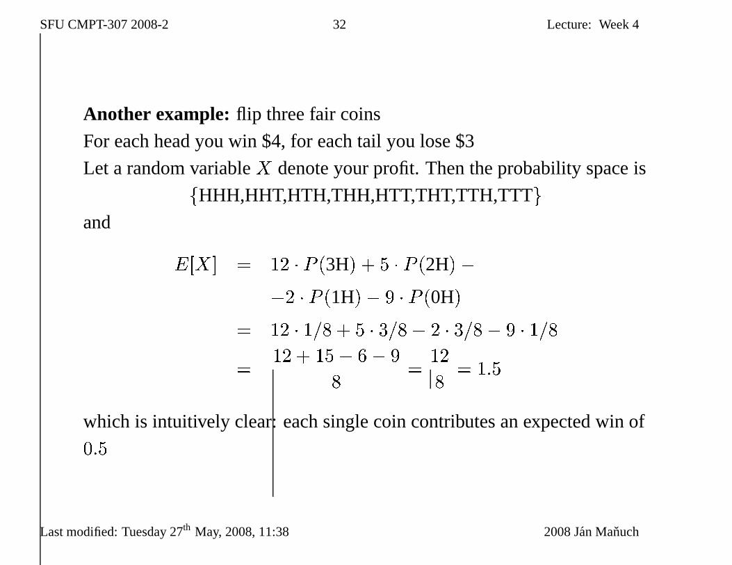
Another example: flip three fair coins
For each head you win $4, for each tail you lose $3
Let a random variableX denote your profit. Then the probability space isfHHH,HHT,HTH,THH,HTT,THT,TTH,TTTg
and E[X℄ = 12 � P (3H) + 5 � P (2H)��2 � P (1H)� 9 � P (0H)= 12 � 1=8 + 5 � 3=8� 2 � 3=8� 9 � 1=8= 12 + 15� 6� 98 = 128 = 1:5which is intuitively clear: each single coin contributes anexpected win of0:5
Last modified: Tuesday 27th May, 2008, 11:38 2008 Jan Manuch

SFU CMPT-307 2008-2 33 Lecture: Week 4
Linearity of expectations
Important: E[X + Y ℄ = E[X℄ + E[Y ℄wheneverE[X℄ andE[Y ℄ are defined
True even ifX andY arenot independent
Last modified: Tuesday 27th May, 2008, 11:38 2008 Jan Manuch
SFU CMPT-307 2008-2 34 Lecture: Week 4
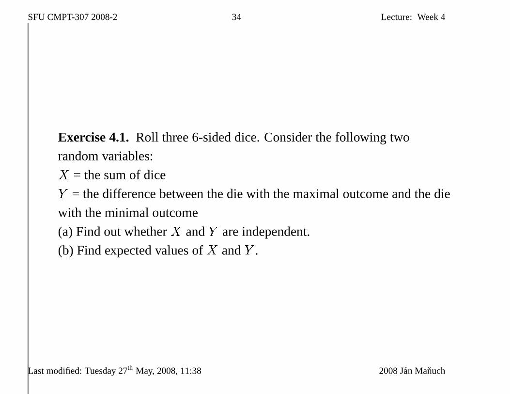
Exercise 4.1.Roll three 6-sided dice. Consider the following two
random variables:X = the sum of diceY = the difference between the die with the maximal outcome andthe die
with the minimal outcome
(a) Find out whetherX andY are independent.
(b) Find expected values ofX andY .
Last modified: Tuesday 27th May, 2008, 11:38 2008 Jan Manuch
SFU CMPT-307 2008-2 35 Lecture: Week 4
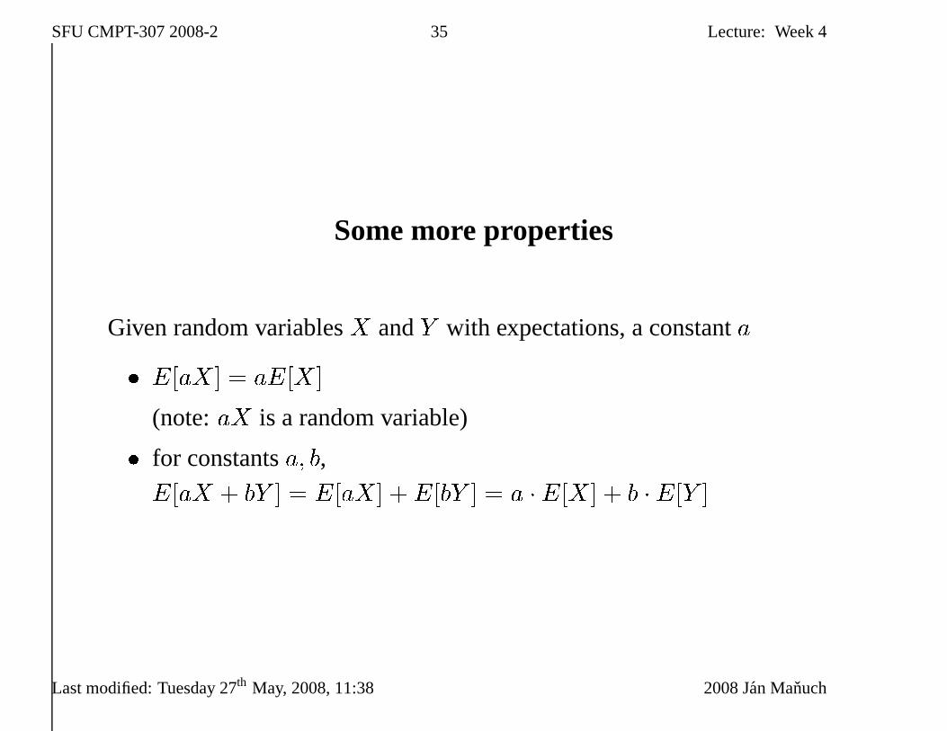
Some more properties
Given random variablesX andY with expectations, a constanta� E[aX℄ = aE[X℄(note:aX is a random variable)� for constantsa; b,E[aX + bY ℄ = E[aX℄ +E[bY ℄ = a �E[X℄ + b �E[Y ℄
Last modified: Tuesday 27th May, 2008, 11:38 2008 Jan Manuch
SFU CMPT-307 2008-2 36 Lecture: Week 4
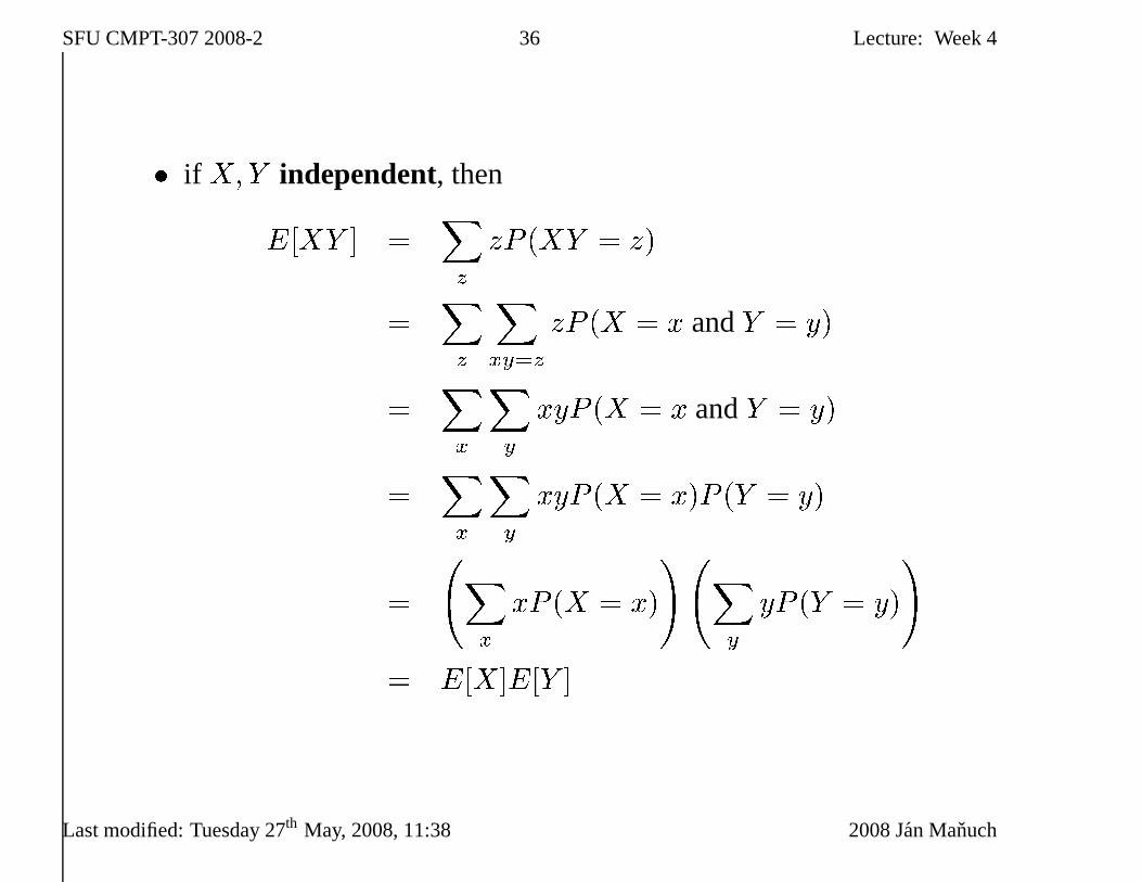
� if X;Y independent, thenE[XY ℄ = Xz zP (XY = z)= Xz Xxy=z zP (X = x andY = y)= Xx Xy xyP (X = x andY = y)= Xx Xy xyP (X = x)P (Y = y)
= Xx xP (X = x)! Xy yP (Y = y)!= E[X℄E[Y ℄
Last modified: Tuesday 27th May, 2008, 11:38 2008 Jan Manuch
SFU CMPT-307 2008-2 37 Lecture: Week 4
Analysis of Randomized-Quicksort
We want to analyseexpected running time
Already have some intuition:
if splits are (more or less) balanced, then good performance
Some observations:� running time is dominated by time spent in Partition()� each time Partition() is called, a pivot is selected� this pivot isnever againincluded in further recursive calls� thus at mostn calls to Partition() overentire execution
Last modified: Tuesday 27th May, 2008, 11:38 2008 Jan Manuch
SFU CMPT-307 2008-2 38 Lecture: Week 4
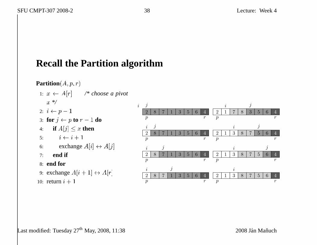
Recall the Partition algorithm
Partition (A; p; r)1: x A[r℄ /* choose a pivotx */
2: i p� 1
3: for j p to r � 1 do4: if A[j℄ � x then5: i i+ 1
6: exchangeA[i℄$ A[j℄7: end if8: end for9: exchangeA[i+ 1℄$ A[r℄
10: returni+ 12 8 7 1 3 5 6 4
p r
i j
2 8 7 1 3 5 6 4
p r
i j
2 8 7 1 3 5 6 4
p r
i j
2 8 7 1 3 5 6 4
p r
i j
2 1 7 8 3 5 6 4
p r
i j
2 1 3 8 7 5 6 4
p r
i j
2 1 3 8 7 5 6 4
p r
i j
2 1 3 8 7 5 6 4
p r
i
Last modified: Tuesday 27th May, 2008, 11:38 2008 Jan Manuch
SFU CMPT-307 2008-2 39 Lecture: Week 4
� one call to Partition() takesO(1) plus amount proportional to # of
iterations of the loop� each iteration compares pivot to some other element� thus boundingtotal # of comparisons yields bound ontotal time
spent in loop (which dominates overall running time)
Lemma. LetX be # of comparisons over entire execution onn-element
array. Then running time isO(n+X).Proof. At mostn calls to partition, each of which� does constant amount of work, and then� executes the loop some # of times
Each iteration of loop performs one comparison
Last modified: Tuesday 27th May, 2008, 11:38 2008 Jan Manuch
SFU CMPT-307 2008-2 40 Lecture: Week 4
Seems we need to boundX, total # of comparisons
Not going to analyze # of comparison ineachcall to Partition(), but rather
total #
Convenience: rename elements ofA asz1; z2; : : : ; zn with zi beingi-thsmallest element.
LetZij = fzi; zi+1; : : : ; zjgQuestion: does algorithm comparezi andzj and how often?
Observation: each pair of elements is comparedat most once(comparisons only to pivot, and that one never again)
Define random variables
Xij = 8<: 1 zi is compared tozj at some time0 otherwise
Last modified: Tuesday 27th May, 2008, 11:38 2008 Jan Manuch

SFU CMPT-307 2008-2 41 Lecture: Week 4
Each pair compared at most once, thusX = n�1Xi=1 nXj=i+1Xij
is total # of comparisons during entire run
Interested in expectations:
E[X℄ = E 24n�1Xi=1 nXj=i+1Xij35 = n�1Xi=1 nXj=i+1E[Xij ℄
= n�1Xi=1 nXj=i+1P (zi is compared tozj)2nd equation is because of linearity of expectation,3rd becauseXij is so-calledBernoulli (or 0� 1) random variable: bydefinition,E[Xij ℄ =Px x � P (Xij = x), and with Bernoulli randomvariable we haveE[Xij ℄ = 0 � P (Xij = 0) + 1 � P (Xij = 1) = P (Xij = 1)
Last modified: Tuesday 27th May, 2008, 11:38 2008 Jan Manuch
SFU CMPT-307 2008-2 42 Lecture: Week 4
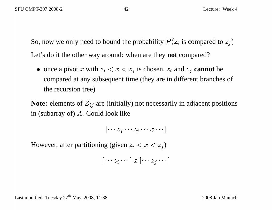
So, now we only need to bound the probabilityP (zi is compared tozj)
Let’s do it the other way around: when are theynot compared?� once a pivotx with zi < x < zj is chosen,zi andzj cannot be
compared at any subsequent time (they are in different branches of
the recursion tree)
Note: elements ofZij are (initially) not necessarily in adjacent positions
in (subarray of)A. Could look like[� � � zj � � � zi � � �x � � � ℄However, after partitioning (givenzi < x < zj)[� � � zi � � � ℄ x [� � � zj � � � ℄
Last modified: Tuesday 27th May, 2008, 11:38 2008 Jan Manuch
SFU CMPT-307 2008-2 43 Lecture: Week 4
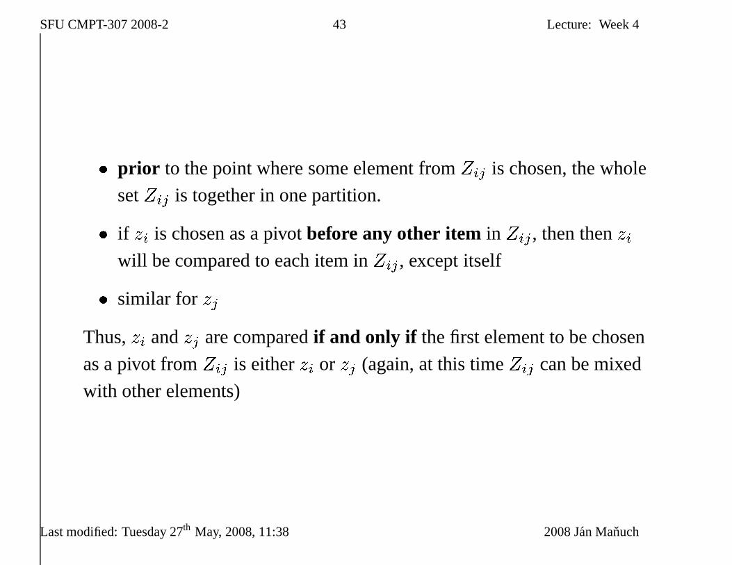
� prior to the point where some element fromZij is chosen, the whole
setZij is together in one partition.� if zi is chosen as a pivotbefore any other item in Zij , then thenzi
will be compared to each item inZij , except itself� similar for zjThus,zi andzj are comparedif and only if the first element to be chosen
as a pivot fromZij is eitherzi or zj (again, at this timeZij can be mixed
with other elements)
Last modified: Tuesday 27th May, 2008, 11:38 2008 Jan Manuch
SFU CMPT-307 2008-2 44 Lecture: Week 4
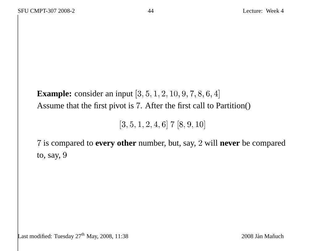
Example: consider an input[3; 5; 1; 2; 10; 9; 7; 8; 6; 4℄
Assume that the first pivot is7. After the first call to Partition()[3; 5; 1; 2; 4; 6℄ 7 [8; 9; 10℄7 is compared toevery othernumber, but, say,2 will never be compared
to, say,9
Last modified: Tuesday 27th May, 2008, 11:38 2008 Jan Manuch

SFU CMPT-307 2008-2 45 Lecture: Week 4
Since elements inZij are in the same partition before any of them is
chosen as a pivot, each one has the same probability of being the first one
chosen (among all fromZij).jZij j = j � i+ 1, thus probability that any given element is the first one
chosen as a pivot is1=(j � i+ 1)Note: This isnot the probability that� a given element is chosen as a pivot during the execution of the
algorithm;� neither that a given element is chosen as a pivot during a (any)
partitioning step;� but it is the probability that a given element is chosen as a pivot
during partitioning in which one of the elements ofZij is chosen as a
pivot.
Last modified: Tuesday 27th May, 2008, 11:38 2008 Jan Manuch
SFU CMPT-307 2008-2 46 Lecture: Week 4
P (zi is compared tozj)= P (zi or zj is first pivot chosen fromZij)(�)= P (zi is first pivot chosen fromZij) +P (zj is first pivot chosen fromZij)= 1j � i+ 1 + 1j � i+ 1= 2j � i+ 1(*) follow because the events are mutually exclusive
Now we haveE[X℄ = n�1Xi=1 nXj=i+1P (zi is compared tozj)
= n�1Xi=1 nXj=i+1 2j � i+ 1Last modified: Tuesday 27th May, 2008, 11:38 2008 Jan Manuch

SFU CMPT-307 2008-2 47 Lecture: Week 4
Let start by replacingj � i with k:
E[X℄ = n�1Xi=1 nXj=i+1 2j � i+ 1 = n�1Xi=1 n�iXk=1 2k + 1
< n�1Xi=1 n�iXk=1 2k = 2 n�1Xi=1 n�iXk=1 1k< 2 n�1Xi=1 nXk=1 1k = 2 n�1Xi=1 O(log n) = O(n log n)
Harmonic number Hn = 1=1 + 1=2 + : : : 1=n.Hn = lnn+O(1) = �(log n)Result: Randomized-Partition yields expected (overall) running time of
Quicksort of orderO(n log n)
Last modified: Tuesday 27th May, 2008, 11:38 2008 Jan Manuch
SFU CMPT-307 2008-2 48 Lecture: Week 4
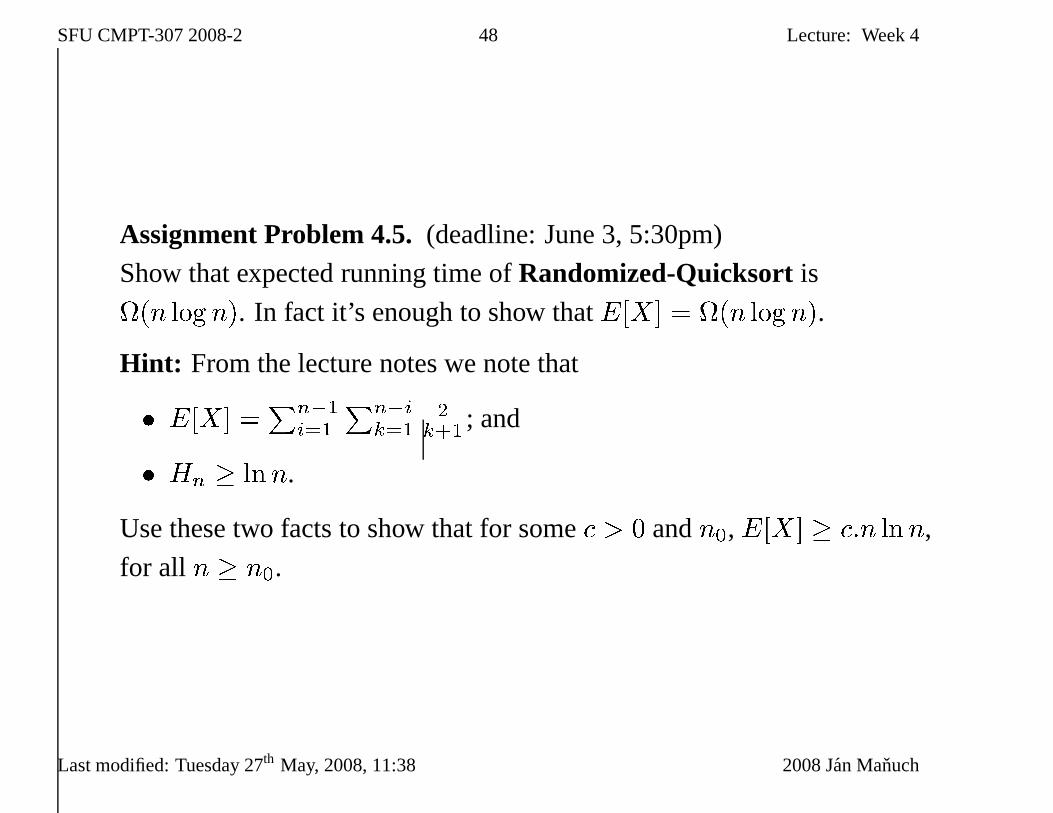
Assignment Problem 4.5.(deadline: June 3, 5:30pm)
Show that expected running time ofRandomized-Quicksort is(n log n). In fact it’s enough to show thatE[X℄ = (n log n).Hint: From the lecture notes we note that� E[X℄ =Pn�1i=1 Pn�ik=1 2k+1 ; and� Hn � lnn.
Use these two facts to show that for some > 0 andn0, E[X℄ � :n lnn,
for all n � n0.Last modified: Tuesday 27th May, 2008, 11:38 2008 Jan Manuch
SFU CMPT-307 2008-2 49 Lecture: Week 4
Note: a difference betweenaverageandexpectedrunning time:� Average running time is the averageover all possible inputs.� Expected running time is, given some input, the average running time
of your randomized algorithm on this inputover all possible random
choices.
Last modified: Tuesday 27th May, 2008, 11:38 2008 Jan Manuch


![SFU, CMPT 741, Fall 2009, Martin Ester 350 Graph Mining and Social Network Analysis Outline Graphs and networks Graph pattern mining [Borgwardt & Yan 2008]](https://img.pdfslide.net/doc/110x75/56649d265503460f949fcaac/sfu-cmpt-741-fall-2009-martin-ester-350-graph-mining-and-social-network.jpg)