1

Shadow Information Spaces:Combinatorial Filters for Tracking Targets

Jingjin Yu Steven M. LaVallejyu18@uiuc.edu lavalle@uiuc.edu

Department of Electrical and Computer Engineering Department of Computer ScienceUniversity of Illinois University of Illinois

Urbana, IL 61801 USA Urbana, IL 61801 USA

Abstract—This paper introduces and solves a problem ofmaintaining the distribution of hidden targets that move outsidethe field of view while a sensor sweep is being performed, result-ing in a generalization of the sensing aspect of visibility-basedpursuit-evasion games. Our solution first applies informationspace concepts to significantly reduce the general complexity sothat information is processed only when the shadow region (allpoints invisible to the sensors) changes combinatorially or targetspass in and out of the field of view. The cases of distinguishable,partially distinguishable, and completely indistinguishable targetsare handled. Depending on whether the targets move nondeter-ministically or probabilistically, more specific classes of problemsare formulated. For each case, efficient filtering algorithms areintroduced, implemented, and demonstrated that provide criticalinformation for tasks such as counting, herding, pursuit-evasion,and situational awareness.

I. INTRODUCTION

Imagine a game of hide-and-seek is being played. Afterthe hiders conceal themselves (subsequent relocations areallowed), the seekers, familiar with the environment, start tosearch for the hiders. Most people who played the game asschoolchildren know that an effective search begins with theseekers checking places having high probabilities of containinga hider, from previous experience: A closet, an attic, a thickbush, and so on. After the most likely locations are exhausted,the next step is to carry out a systematic search of theenvironment, possibly with some seekers guarding certainescape routes. Occasionally, during the game, hiders mayattempt to relocate themselves to avoid being found. Whilethe hiders succeed sometimes, they may end up being spottedby the seekers and are instead getting found earlier.

Although a child’s play, this game captures the two keyinteracting ingredients of pursuit evasion (PE) games: Pas-sively estimating the distribution of hidden targets and activelyplaning to reduce the uncertainty of this distribution. Thegeneral goal in PE research is to algorithmically clear evadingtargets from a workspace. As pursuers try to ensure that theworkspace is evader-free, they always need to maintain thepursuit status, remembering whether a region outside of thepursuers’ field-of-view (FOV) is contaminated or cleared (onebit of information per region).

This paper, expanding upon [51], [52], studies exactly thispassive ingredient of PE games, reasoning about the informa-tion residing in unobservable regions of the environment. In

particular, we introduce the notion of filters over shadow in-formation spaces for tracking moving targets in unobservableregions, as a generalization of this aspect of PE. To achievethis, we first process sensor observation history and compressit in a lossless fashion for our task classes, for storage andeffective computation. Next, depending on whether the targetsof interest are moving nondeterministically or probabilistically,concrete problems are formulated and solved by carefullymanipulating and fusing observation and data. At a higherlevel, at any time, our algorithm can estimate the numberof targets hidden in regions not directly observable. We notethat, although the active problem of planning a pursuit path isnot addressed in this work, heuristic search strategies can bereadily implemented on the space of filter outputs.

The mathematical study of PE games dates back to at leastfour decades ago, with its roots in differential games [15]–[17].Although optimal strategies for differential PE games are stillactively pursued [2], [25], [29], [46], a variant of differentialPE games, visibility based PE, has received much attentionrecently. Development of visibility based PE games can betraced back to [32], in which a PE game on discrete graphis introduced with the goal of sweeping evaders residing oncontinuous edges of a graph. The evaders can move arbitrarilyfast, but must move continuously. The Watchman Route prob-lem [8], [9], formulated twelve years later as a variant of theArt Gallery problems [27], [38], involves finding shortest routeto clear static intruders. An intruder is considered cleared ifa line of sight exists between the intruder and a point of thewatchman route.

Influenced by these two threads of research, [42] definedwhat we know today as visibility based PE games in whichthe discrete graph domain is replaced by a path connectedinterior of a 2D polygon and a continuously moving evaderis considered to be cleared if it falls into the visible regionof a pursuer (in this case the pursuer is equipped with twoflashlights and is called a 2-searcher). Thinking along the samelines as the Art Gallery problems, it was soon established thatfor a pursuer with an omnidirectional infinite range sensor (an∞-searcher), it is NP-hard to decide the minimum number ofpursuers needed for the class of simply connected polygons[14], [24]. The insight that bitangents and inflections fullycapture the critical changes leads to a generalization frompolygons to curved environments [23] and form the basis of

2

some critical events used in our work.Various sensing and motion capabilities are explored in vis-

ibility based PE. Interestingly, it turns out that a 2-searcher isas capable as an ∞-searcher in simple polygons [31]. Pursuerswith a single flashlight/beam (a 1-searcher) are investigated indetail in [39] and [20], with the latter limiting the pursuer’smotion to the boundary of the environment. Variations alongthis line include limited FOV [11], unknown environments[35], and bounded speed [44]. Another theme in PE gamesis to discretize time and put speed bounds on both pursuersand evaders. In this setting, sufficient conditions and strategiesfor a single pursuer to capture an evader are given to theclassical lion-and-man problem in the first quadrant of theopen plane [37]. This problem is then extended to R

n andmultiple pursuers in [21], and multiple pursuers with limitedrange in [5]. Finally, PE is also studied in the probabilisticcontext [18], [47] and abstract metric spaces [1].

Since we provide algorithms for tracking moving targets,our work is also closely related to target tracking and enu-meration. The problem of accurately counting the numberof targets with overlapping footprints is solved with a novelapproach of integrating over Euler characteristics in [3]. Witha virtual sensor that reports visible features of polygonalenvironment as well as indistinguishable targets, static targetsare counted under various setups in [12]. A filtering algorithmis provided in [40] to count moving targets with a network ofbinary proximity sensors. In [48], Simultaneous Localizationand Mapping (SLAM) and Detection and Tracking of MovingObjects (DTMO) are combined to attack both problems at thesame time. A specialization of our problem is investigatedin [43] in which the sensor FOV becomes one dimensionalbeams. Real-time people counting with a network of imagesensors is studied in [50].

Another research area of relevance to this paper, especiallythe probabilistic formulations we give in Section VI, is thestudy of optimal search [41], which proposes a Bayesianapproach for maintaining a target distribution and use thatinformation for guiding the planning of optimal search paths.The essential idea from optimal search is to plan a pathto eliminate regions with highest probability of containingthe targets. In doing so, optimal search algorithms allow theprediction of the no-detection likelihood [4], [7], [26], [49],which is the probability that the targets remain undiscovered atgiven stages of a search effort, even before the actual search iscarried out. Although our work also seeks to maintain a targetdistribution along a given path, we focus on the computationalproblem of how topological changes of non observable compo-nents, which are combinatorial in nature, can be correctly andefficiently processed as the target distribution evolves. Thistopological/combinatorial element of target tracking existswhether the problem formulation is probabilistic or not. In thisaspect, the problems we address here are mostly orthogonal toclassical optimal search problems, which cover environments(support surfaces of the distribution) that are mainly twodimensional, obstacle-less planes such as these appearing intypical maritime applications. As such, the results presentedin this paper should benefit the extension of optimal searchresults to covering more diverse workspaces such as urban

areas and hilly terrains, where topological changes of nonobservable components are frequent.

The main contributions of this work are twofold. First, asexplained above, we generalize visibility based PE by intro-ducing a richer class of problems and providing a frameworkas a submodule for systematically attacking these problems.Second, the capability of effectively tracking hidden, movingtargets, a general type of situation awareness, applies to a largeclass of time critical tasks in both civilian and national secu-rity applications. For example, in a fire evacuation scenario,knowing the the possible/expected number of people trappedin various parts of a building, firefighters can better decidewhich part of the building should be given priority when theycoordinate the search and rescue effort.

The rest of the paper is organized as follows. SectionII provides a mathematical definition of what we mean by“shadows” and “component events”, which can be best cap-tured using a chronological sequence. Section III suggests thegeneral problem of tracking hidden targets after bringing inmoving targets and FOV events, . Section IV formulates theproblem of estimating the number of targets hidden in shadowsfor nondeterministically moving targets and establishes itspolynomial time solvability using results from integer linearprogramming theory. Section V shows how information spaces[22] can guide the design of efficient algorithms for solvingthe nondeterministic formulation in a more intuitive fashion.Section VI extends the problem formulation and solutions toprobabilistically moving targets and imperfect sensors. Weprovide implementation, simulation results, and algorithmicanalysis in Section VII, and conclude with Section VIII.

II. COMPONENT EVENTS, SHADOWS, AND SHADOW

SEQUENCES

Intuitively, in the hide-and-seek game, the part of the worldthat is not observable is comprised of many components, eachof which has a life span. To study the information flow inthem, a formal definition of components is first in order; thetemporal relationship among them then naturally comes up.

A. Component events and shadows

Let a nonempty set of robots move along continuous tra-jectories in a workspace, W = R

2 or W = R3. Let the

configuration space of the robots be C. At some time t, theremay be configuration space obstacles Cobs which may varyover time, leaving Cfree := C\Cobs as the free configurationspace. Let q ∈ Cfree be the configuration of the robots attime t. Returning to the workspace, there is a closed obstacleregion O(t) ⊂ W , leaving F (t) := W\O(t) as the freespace. The robots are equipped with sensors that allow themto make shared observations in a joint FOV or visible regionV (q, t) ⊂ F (t). For convenience, we take the closure ofV (q, t) and assume that the visible region is always closed.Let S(q, t) := F (t)\V (q, t) be the shadow region, which maycontain zero or more nonempty path connected components(path components for short). A path component is assumedto be nonempty unless otherwise specified. At any instant,O(t), V (q, t), and S(q, t) have disjoint interiors by definition

3

and W = O(t) ∪ V (q, t) ∪ S(q, t). Fig. 1 shows V (q), S(q)for a point robot holding a flashlight with F ⊂ W = R

2,Cfree ⊂ SE(2), which is the set of two dimensional transla-tions and rotations (here we omit the parameter t from F, V ,and S since the obstacle region does not vary over time).

F q

V(q)

s1

s2

S(q)

(a) (b) (c)

Fig. 1. (a) The environment and the free space, F . Note that in this example,the obstacle region is fixed; therefore, F is constant. (b) The visible region,V (q). (c) The shadow region, S(q), with two path components s1, s2.

To observe how path components of the shadow regionevolve over time, let the robots follow some path τ : [t0, tf ] →C in which [t0, tf ] ⊂ T ⊂ R is a time interval. Let Z = W×T .We may let O : T → Pow(Z) be the map that yields theobstacle region and define V, S as:

V, S : C × T → Pow(Z).

Since a path τ , parameterized over t ∈ T , is always as-sumed in the paper, we abusively write V (t), S(t) in placeof V (τ(t), t), S(τ(t), t), respectively. In particular, we areinterested in S(t) and call it a slice. For any (ta, tb) ⊂ [t0, tf ],let the union of all slices over the interval,

S(ta, tb) :=⋃

t∈(ta,tb)

S(t),

be called a slab, which is an open subset of Z . For any subsetz of Z , define its projection onto the time axis as

πt : Pow(Z) → Pow(T ),z �→ {t | (p, t) ∈ z for some p ∈ W}.

Let st,i ⊂ S(t) denote the i-th path component of S(t) (as-suming some arbitrary ordering). Let s i′ denote the i′-th pathcomponent of a slab S(ta, tb) (again, assuming some arbitraryordering). S(ta, tb) is homogeneous if for all t ∈ (ta, tb) andall i, there exists i′ such that

st,i = S(t) ∩ si′ ,

and separately,

πt(si′) = (ta, tb) for all i′.

A homogeneous slab is called maximal if it is not a propersubset of another homogeneous slab. The definition then parti-tions S(t0, tf ) into some m disjoint maximally homogeneousslabs plus some slices

S(t0, tf ) = S(t0, t1) ∪ S(t1) ∪ . . . ∪ S(tm−1) ∪ S(tm−1, tf ).

That is, homogeneity of S(t0, tf ) is broken at t1, . . . , tm−1.What exactly happens at t1, . . . , tm−1? Let there be twohomogeneous slabs S(ta, tb) and S(tb, tc) such that for somek ∈ {1, . . . ,m − 1}, tk−1 ≤ ta < tb = tk < tc ≤ tk+1. Letsi be an arbitrary path component of S(ta, tb), at t = tb, simay (s denotes the closure of s)

1) live on, if there exists a path component sj ⊂ S(tb, tc)such that si ∩ S(tb) = sj ∩ S(tb) = ∅.

2) disappear, if si ∩ S(tb) = ∅.

Similarly, a path component sj ⊂ S(tb, tc) may

3) appear, if sj ∩ S(tb) = ∅.

Finally, a nonempty set of path components {s i} of S(ta, tb)may

4) evolve, if there is a nonempty set of path components{sj} of S(tb, tc) such that |{si}|+|{sj}| ≥ 3 and

⋃i si∩

S(tb) =⋃

j sj ∩ S(tb) = ∅ is a single path componentof S(tb).

By definition, appear, disappear, and evolve are criticalchanges that only (and at least one of which must) happenbetween two adjacent maximally homogeneous slabs. We callthese changes component events. With component events,homogeneity and maximality readily extend to path compo-nents of slabs. A path component si ⊂ S(ta, tb) is calledhomogeneous if no component events happen to a subset ofsi in (ta, tb); si is called maximal if it is not a proper subsetof another homogeneous path component.

W

t1 t4t3t2t0 tf

s6

s5s4

s3

s2

s1

T

Fig. 2. Evolution of shadows: t1: s3 appears, t2: s2, s3 merge into s4, t3:s4 splits into s5, s6, t4: s6 disappears. The “sizes” of the shadows have noeffect on the critical events.

At this point, a type of general position is assumed to avoidtwo tedious cases: 1) Four or more path components cannot beinvolved in an evolve event, and 2) Two or more componentevents cannot occur at the same time. In practice, non generalposition scenarios form a measure zero set and can be dealtwith via small perturbations to the input if required. Withsuch an assumption, exactly one component event happensbetween two maximally homogeneous slabs. Moreover, theevolve event can be divided into two sub events: split if|{si}| = 1, |{sj}| = 2 and merge if |{si}| = 2, |{sj}| = 1.

We now piece together the above definitions using anexample illustrated in Fig. 2. Restricting to the time inter-val (t0, tf ), there are five maximally homogeneous slabs,S(t0, t1), . . . , S(t4, tf ). Certain proper subsets of one of these,such as S(t+2 , t

−3 ) with t2 < t+2 < t−3 < t3, are again

homogeneous but no longer maximal; on the other hand,supersets such as S(t−2 , t

+3 ) with t−2 < t2 < t3 < t+3 , are

no longer homogeneous. The slab S(t0, tf) ⊂ Z has two pathcomponents (s1 and Int(s2 ∪ s3 ∪ s4 ∪ s5 ∪ s6), in which Intdenotes the interior of a set) and six maximally homogeneouspath components s1, . . . , s6. The intersection of a vertical lineat t ∈ (t0, tf ) with S(t0, tf ) corresponds to the slice S(t).For convenience, it is assumed that t = t0 is not a criticaltime in the sense that for each path component s t0,i ⊂ S(t0),

4

st0,i = si′ ∩ S(t0) for some path component si′ ⊂ S(t0, t1).A similar assumption is made for t = tf . Under this setup,there are four component events: 1. s3 appears at t = t1; 2.s2 and s3 merge to form s4 at t = t2; 3. s4 splits into s5, s6at t = t3; and 4. s6 disappears at t = t4. In contrast, the pathcomponent s1 ∩ S(t0, t1) lives on through t1, . . . , t4.

Finally in this subsection, we define the main concept ofthe paper: shadow. It is easy to see that maximally homo-geneous path components are pairwise disjoint. Let such apath component be called a shadow and let {s i} be the set ofshadows of S(t0, tf ); note that S(t0, tf ) is contained in theclosure of ∪isi. In the above example, {si} = {s1, . . . , s6}.For some t ∈ (t0, tf ), let a path component of S(t) belabeled as st,i if it is a slice of a shadow si. More precisely,st,i = si ∩ {(p, t) | p ∈ W}. For t = t0, st0,i is labeled suchthat st0,i = si∩S(t0) for some path component si ⊂ S(t0, t1).The same applies to the labeling of stf ,i. A path component ofS(t) has no label exactly when it is the border of two or moreshadows of a slab. Since such labeling is unique, we drop timesubscript of st,i if t is fixed. In the rest of the paper, we usethe set {si} to denote both shadows and slices of shadows;we simply call both types of path components shadows whenno confusion arises from the context. When we do need todistinguish, the former will be called workspace-time shadowsand the later workspace shadows.

B. Shadows are everywhere

s2

s1

s3 s2

s1

(a) (b) (c)s1

s4

s1

s6s5 s5

s1

(d) (e) (f)

Fig. 3. An example of shadows and their indexing/labeling. (a) The setof spotlights and the path to be followed by the darker (orange) coloredspotlight. (b) Initially, only shadow s2 and unbounded shadow s1 exist. (c)A new shadow s3 appears. (d) s2, s3 merge into a single shadow s4. (e) s4splits into new shadows s5, s6. (f) s6 disappears.

To promote the intuition behind the mathematical defini-tions, let us look at a realistic example shown in Fig. 3(a).With the intention of guarding a planar region, spotlights arecast on the ground, creating a set of illuminated discs asshown. Assume that only the darker (orange) colored disc oflight moves and follows the dashed line. For any position ofthe moving spotlight, the combined, illuminated set can bethought of as the FOV. Its complement in the plane is theshadow region, in which targets cannot be directly observed.Initially, there are two connected components, labeled s 1

(unbounded) and s2, in the shadow region. As the spotlightmoves along the dashed line, we observe that shadows mayappear, disappear, merge, and split, as illustrated in Fig. 3(b)to (f). We constructed this example so that the events and

evolution of shadows match exactly these of the example fromFig. 2.

The naive example suggests that shadows and componentevents arise from very simple setups. Indeed, shadows andcomponent events are ubiquitous, showing up whenever mov-ing sensors are placed inside environments. We provide threeadditional examples to corroborate this point; many otherscould be presented. In Fig. 4(a), omni-directional, infiniterange sensors partition the 2D environment into polygonalshadows. The component events happen exactly when thesensors make inflection and bitangent crossings (see aspectgraphs [33]), which gives rises to the concept of gaps and gapnavigation trees as discussed in [45]. If the sensors have lim-ited viewing angle [11] or limited range (Fig. 4(b)), alternatemodels governing visible and shadow regions are obtained. InFig. 4(c), fixed infrared beams and surveillance cameras areplaced inside a building, creating a set of three fixed shadowss1, s2, s3. Such a setting is common in offices, museums, andshopping malls. As a last example, Fig. 4(d) shows a simplifiedmobile sensor network with coverage holes. In this case, thejoint sensing range of the sensor nodes is the FOV and thecoverage holes are the shadows, which fluctuate continuouslyeven if the sensor nodes remain stationary (consider cellphonesignals).

s4

s1

s5

s2 s3

s6 s7

s1

s2

(a) (b)

s1 s2 s3

s1 s2

(c) (d)

Fig. 4. a) Two robots (white discs) carrying omni-directional, infinite rangesensors. The free space is partitioned into seven shadows. b) When sensingrange is limited, the topology of shadows changes; only two shadows are left.c) An indoor environment guarded by fixed beam sensors (red line segments)and cameras (yellow cones). There are three connected shadows. d) A simplemobile sensor network in which the white discs are mobile sensing nodes,with shaded regions being their sensing range at the moment. There are twoshadows with s1 being unbounded.

For some environments, shadows are readily available or canbe effectively computed with high accuracy, such as visibilitysensors placed in 2D polygonal environments. In some othercases, shadows are not always easy to extract. As one example,estimating coverage holes in a wireless sensor network israther hard since it is virtually impossible to know whethera point p is covered unless a probe is dispatched to p tocheck. It is also well known that 3D visibility structure isdifficult to compute [28], [34]. Even though we do not claimto overcome such inherent difficulties in acquiring visibilityregion and/or shadows, the method presented here applies as

5

long as a reasonably accurate characterization of the shadowsis available.

C. Shadow sequences

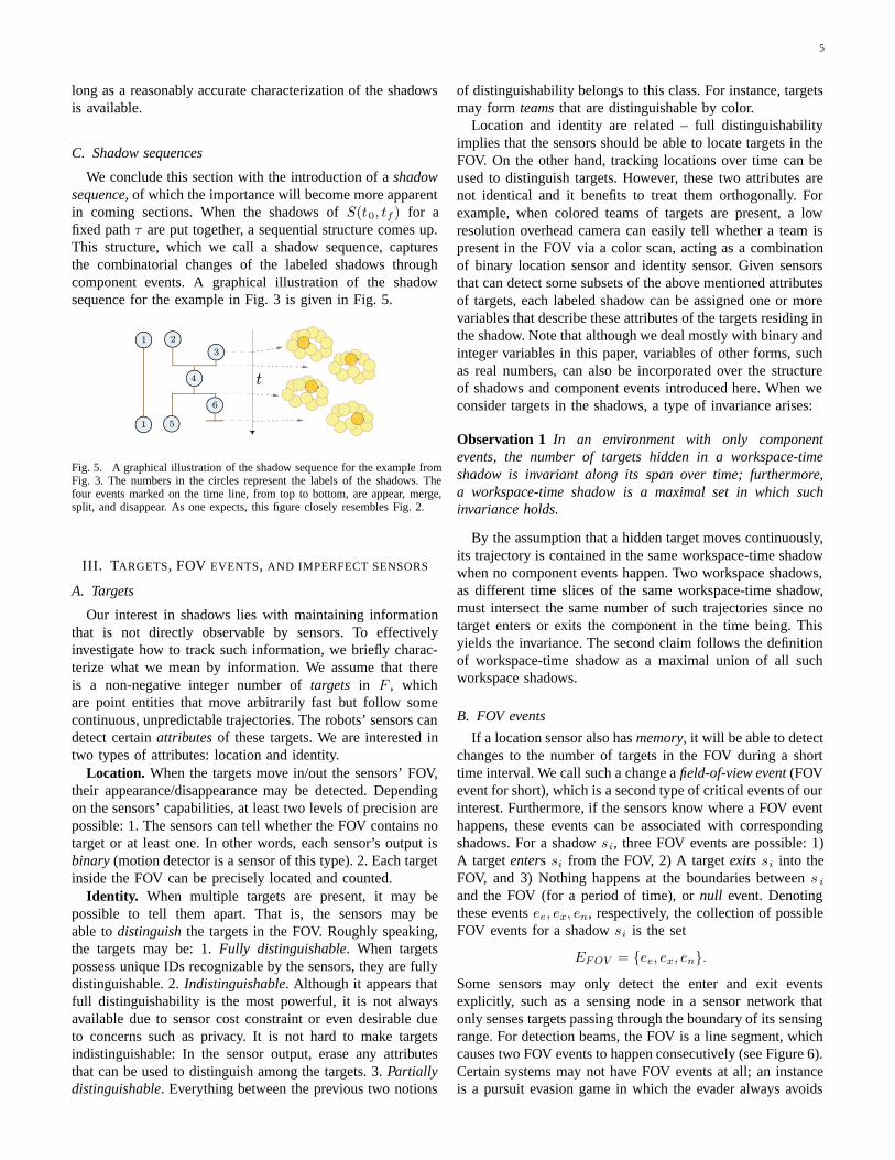
We conclude this section with the introduction of a shadowsequence, of which the importance will become more apparentin coming sections. When the shadows of S(t0, tf ) for afixed path τ are put together, a sequential structure comes up.This structure, which we call a shadow sequence, capturesthe combinatorial changes of the labeled shadows throughcomponent events. A graphical illustration of the shadowsequence for the example in Fig. 3 is given in Fig. 5.

2

t4

6

5

3

1

1

Fig. 5. A graphical illustration of the shadow sequence for the example fromFig. 3. The numbers in the circles represent the labels of the shadows. Thefour events marked on the time line, from top to bottom, are appear, merge,split, and disappear. As one expects, this figure closely resembles Fig. 2.

III. TARGETS, FOV EVENTS, AND IMPERFECT SENSORS

A. Targets

Our interest in shadows lies with maintaining informationthat is not directly observable by sensors. To effectivelyinvestigate how to track such information, we briefly charac-terize what we mean by information. We assume that thereis a non-negative integer number of targets in F , whichare point entities that move arbitrarily fast but follow somecontinuous, unpredictable trajectories. The robots’ sensors candetect certain attributes of these targets. We are interested intwo types of attributes: location and identity.

Location. When the targets move in/out the sensors’ FOV,their appearance/disappearance may be detected. Dependingon the sensors’ capabilities, at least two levels of precision arepossible: 1. The sensors can tell whether the FOV contains notarget or at least one. In other words, each sensor’s output isbinary (motion detector is a sensor of this type). 2. Each targetinside the FOV can be precisely located and counted.

Identity. When multiple targets are present, it may bepossible to tell them apart. That is, the sensors may beable to distinguish the targets in the FOV. Roughly speaking,the targets may be: 1. Fully distinguishable. When targetspossess unique IDs recognizable by the sensors, they are fullydistinguishable. 2. Indistinguishable. Although it appears thatfull distinguishability is the most powerful, it is not alwaysavailable due to sensor cost constraint or even desirable dueto concerns such as privacy. It is not hard to make targetsindistinguishable: In the sensor output, erase any attributesthat can be used to distinguish among the targets. 3. Partiallydistinguishable. Everything between the previous two notions

of distinguishability belongs to this class. For instance, targetsmay form teams that are distinguishable by color.

Location and identity are related – full distinguishabilityimplies that the sensors should be able to locate targets in theFOV. On the other hand, tracking locations over time can beused to distinguish targets. However, these two attributes arenot identical and it benefits to treat them orthogonally. Forexample, when colored teams of targets are present, a lowresolution overhead camera can easily tell whether a team ispresent in the FOV via a color scan, acting as a combinationof binary location sensor and identity sensor. Given sensorsthat can detect some subsets of the above mentioned attributesof targets, each labeled shadow can be assigned one or morevariables that describe these attributes of the targets residing inthe shadow. Note that although we deal mostly with binary andinteger variables in this paper, variables of other forms, suchas real numbers, can also be incorporated over the structureof shadows and component events introduced here. When weconsider targets in the shadows, a type of invariance arises:

Observation 1 In an environment with only componentevents, the number of targets hidden in a workspace-timeshadow is invariant along its span over time; furthermore,a workspace-time shadow is a maximal set in which suchinvariance holds.

By the assumption that a hidden target moves continuously,its trajectory is contained in the same workspace-time shadowwhen no component events happen. Two workspace shadows,as different time slices of the same workspace-time shadow,must intersect the same number of such trajectories since notarget enters or exits the component in the time being. Thisyields the invariance. The second claim follows the definitionof workspace-time shadow as a maximal union of all suchworkspace shadows.

B. FOV events

If a location sensor also has memory, it will be able to detectchanges to the number of targets in the FOV during a shorttime interval. We call such a change a field-of-view event (FOVevent for short), which is a second type of critical events of ourinterest. Furthermore, if the sensors know where a FOV eventhappens, these events can be associated with correspondingshadows. For a shadow si, three FOV events are possible: 1)A target enters si from the FOV, 2) A target exits si into theFOV, and 3) Nothing happens at the boundaries between s i

and the FOV (for a period of time), or null event. Denotingthese events ee, ex, en, respectively, the collection of possibleFOV events for a shadow si is the set

EFOV = {ee, ex, en}.Some sensors may only detect the enter and exit eventsexplicitly, such as a sensing node in a sensor network thatonly senses targets passing through the boundary of its sensingrange. For detection beams, the FOV is a line segment, whichcauses two FOV events to happen consecutively (see Figure 6).Certain systems may not have FOV events at all; an instanceis a pursuit evasion game in which the evader always avoids

6

321

Fig. 6. Illustration of FOV events for an environment with obstructedvisibility (left) and for an environment with detection beams (right). 1) Atarget is about to exit a shadow into the FOV of the sensor (yellow disc). 2)A target is about to enter a shadow from the sensor’s FOV. 3) A target isabout to enter and exit the FOV of a beam sensor.

appearing in the pursuer’s FOV. The game ends when anevader is found or when it is confirmed that no evader is inthe environment.

1

7

time

65

11

10

8

7

3

2

4

4

9

ex

ee

ee

ex

ex

Fig. 7. A typical sequence of critical events. The circles with numbersrepresent the shadows; the labeled arrows associate FOV events to shadows.

Since component events and FOV events both happen asrobots move along some path τ in the free space F , it makessense to treat them as a whole. It does not take much torepresent them together: We can simply augment the shadowsequence to include the FOV events. A typical combinedsequence of critical events is shown in Fig. 7. To incorporateFOV events, the invariance from Observation 1 needs to beupdated.

Observation 2 In an environment with component and FOVevents, the number of targets hidden in a workspace-timeshadow is invariant between FOV events (excluding nullevents) associated with the shadow; the time span of suchinvariance is again maximal.

To see why the above statement is true, note that an enterFOV event can be viewed as an appear component eventimmediately followed by a merge component event. Samebreakdown holds for exit FOV events. The case is then reducedto Observation 1. Observation 2 establishes that for the taskof tracking hidden targets that move continuously, any sensordata unrelated to critical events can be safety discarded withoutadverse effects.

C. The problem of tracking hidden targets

With the introduction of component and FOV events, we canformally define the general problem of tracking hidden targetsthat move continuously. The following inputs are assumed:

1) An initial distribution of targets (in shadows) whose totalnumber remains invariant,

2) An ordered sequence of component and FOV events forthe time interval [t0, tf ], and

3) Any target motion dynamics (for example, nondeter-ministic) that may provide additional information aboutcritical events.

From these inputs, the task is to track the evolution of thetarget distribution and in particular, to estimate at t = tfthe possible number of targets in a given set of shadows.For the rest of this paper, we focus on two flavors of thisproblem: 1) A nondeterministic setting in which targets movenondeterministically but critical events are observed withouterror, and 2) A probabilistic setting in which the targets’movement has a probabilistic model and there are imperfectsensors.

IV. TRACKING NONDETERMINISTICALLY MOVING

TARGETS: THE FORMULATION AND AN ILP PERSPECTIVE

A. Problem formulation

In the nondeterministic setting, we assume that the targetsmove nondeterministically. In particular, when a shadow s i

splits into shadows sj , sk, the targets inside si can splitin any possible way as long as the numbers of targets insj , sk are both nonnegative. The component events and FOVevents are assumed to be observed without error. Given suchassumptions, the observation history can be partitioned intotwo inputs to our filter algorithm:

1) A sequence of shadow and FOV events, and2) The initial conditions of targets in the shadows at time

t = t0.

A typical initial condition for a shadow takes the form

{(a1, l1, u1), (a2, l2, u2), . . . , (ak, lk, uk)}, (1)

in which ai denotes a subset of target attributes (such ashaving red color). We assume that elements of the set {a i}for a shadow are pairwise disjoint: If ai has red color, thenno aj , j = i can include targets with the attribute of havingred color. The corresponding l i and ui denote the lower andupper bounds on the number of targets in the shadow withattribute ai. For example, we may know that at the beginning,a shadow have 6 to 9 green targets and 5 targets that may beblue or red. In this case, the initial condition can be writtenas

{(c = green, 6, 9), (c = blue or red, 5, 5)}.With these inputs, the main task is to determine the lower andupper bounds on the number of targets in any given set ofshadows at t = tf for any combinations of attributes. Theseobtained bounds are always tight in the sense that any targetdistribution falling in these bounds is a possible outcome giventhe initial condition and the observation history.

To make the explanation of the algorithm clear, we firstwork with a single attribute and ignore FOV events. We alsoassume for the moment that the initial conditions are tight inthe sense that all possible choices of values must be consistentwith the later observations (for example, we cannot have ainitial condition of 4 to 6 targets in a shadow and later find thatit is only possible to have 2 targets in it). We will then show

7

how FOV events, multiple attributes, and other extensions canbe handled incrementally.

B. An integer linear programming (ILP) perspective

For the simplest case, since there is a single attribute andthe FOV events are ignored, we can represent the number oftargets in a shadow with a single unknown quantity. Let theset of shadows be {si}; we denote the set of correspondingunknowns as {xi}. We can write the initial condition for eachshadow at t = t0 as two constraints

li ≤ xi ≤ ui. (2)

For each event in the sequence of component events, we thenobtain one extra constraint of the following form:

Appear or disappear: xi = diSplit or merge: xi = xj + xk.

(3)

Here we allow that as an appear event happens, d i targets mayhide in si at the same time. This is more general than lettingdi = 0. To unify notation, we write these in the same way asthe initial conditions by letting li = ui = di. The same appliesto the disappear events. Additionally, we have for each shadowsi, the constraint

xi ≥ 0. (4)

Finally, the task becomes finding the lower and upper boundsof targets for a set of shadows at time t = tf indexed by I.For the upper bound, we can write the problem as maximizingthe sum of the set of unknowns

maximize∑i∈I

xi. (5)

Finding the lower bound then becomes maximizing the set ofunknowns not indexed by I because the total number of targetsare preserved. We have obtained an integer linear program-ming (ILP) problem: All critical events can be expressed usingconstraints of forms from (2),(3) and (4), with the objectivefunction having the form from (5). For example, if we are toexpress the ILP problem in the canonical form, all we need todo is to split each equality constraint (given by (3)) into twoinequality constraints (for example, xi = di becomes xi ≤ diand xi ≥ di) and multiply all inequality constraints with −1where necessary (xi ≤ di ⇒ −xi ≥ −di). This gives us theILP problem in canonical form,

minimize∑i∈I

−xi, subject to Ax ≥ b, x ≥ 0, (6)

in which A is the constraint coefficient matrix accumulatedfrom initial condition and the critical events; x is the vector ofunknowns (one for each shadow). The size of A is determinedby the number of shadows and the number of critical events.For additional discussion on ILP modeling, see [30].

C. Polynomial time solvability of the ILP problem

It is well known that the class of ILP problems is NP-complete in general. It turns out, however, that our ILPproblem is not only feasible, but also efficiently solvable. Wepoint out that an actual target tracking problem may require

solving more than a pair (upper and lower bounds) of ILPproblems as formulated in 6. For example, in a fire rescuescenario, it may be necessary to estimate upper and lowerbounds on all current shadows individually. Nevertheless, aslong as the number of ILP problems are manageable (say,linear with respect to the size of the inputs), the overallproblem can also be efficiently solved.

Proposition 3 A polynomial time algorithm exists for thesystem described by (6).

As a first step in proving the proposition, we establish thefollowing lemma:

Lemma 4 The constraint matrix A in (6) is totally unimodu-lar1.

PROOF. We use induction over the size of square submatricesof A to prove that all such submatrices must have determinant0 or ±1. As the base case, every element of A is 0 or±1. Suppose that all square submatrices of order n havedeterminant 0,±1. Denote these matrices Mn. Supposethere is a square submatrix M of A of order (n + 1) withdeterminant not in {0,±1}. Every constraint arising from (2),(3), and (4) except xi = xj + xk introduces rows in A witha single ±1 in them; the rest of the row contains only 0s. IfM contains a row arising from these types of constraint thenM must have determinant 0,±1 by induction. Suppose not.In this case, all rows of M are introduced by constraint oftype xi = xj + xk. Each such constraint brings in two rowsof A with opposite signs and therefore cannot both appearin M . We can assume that M ’s first row have coefficientscoming from one of the rows introduced by a split event,xi = xj + xk. As a first case, let the i, j, kth columns of Acorrespond to i′, j′, k′th columns of M , respectively. To makeM ’s determinant not in {0,±1}, there needs to be anotherrow in M that contains exactly two non zero elements amongi′, j′, k′th columns. This is only possible if sj and sk mergeagain, giving a constraint of the form xj + xk = xl. Wemay let this row be the second row in M . This suggests thatj′, k′th column of M are all zeros after the second row; butthis gives us that M has determinant 0. The second case isthat M includes only two columns of A’s i, j, kth columns. Itcan be checked similarly that M must have determinant 0. �

PROOF OF PROPSITION 3. When the constraint matrix Ais totally unimodular and b is a vector of integers, thenthe minimal faces of the constraint polytope must assumeinteger coordinates, making the solution of the relaxed linearprogramming (LP) problem also the solution to the originalILP problem [36]. It is clear that b in (6) is integer. Lemma 4gives us that A is totally unimodular. Therefore, a polynomialtime algorithm such as interior point method can be appliedto solve (6). �

1An integer square matrix A is unimodular if detA = ±1. A matrix B istotally unimodular if every non-singular square submatrix of B is unimodular.

8

V. TRACKING NONDETERMINISTICALLY MOVING

TARGETS: AN INFORMATION SPACE PERSPECTIVE AND

EFFICIENT ALGORITHMS VIA COMBINATORIAL FILTERS

Although Proposition 3 tells us that the nondeterministicformulation can be solved in polynomial time using genericLP algorithms, it is not clear that these algorithms fully explorethe intrinsic structure of the problem at hand. In this section,we briefly review the information space (I-space for short, seeChapter 11 of [22] for an introduction) and show how the I-space framework can help with the systematic exploration ofthe structure of filtering problems that are combinatorial innature. For our particular problem, we show that additionalinformation can be discarded from the shadow sequence toyield a further condensed information state (I-state). Algorith-mic solutions based on max-flow are then introduced, followedby various extensions.

A. Information space as a guiding principle for task baseddata filtering

As a shadow sequence is extracted from an observationhistory, a much condensed combinatorial structure is left.This choice is not arbitrary: The general task of trackingunpredictable targets outside the sensor range induces anequivalence relation over the workspace-time space that yieldsthe space of shadows; the evolution of these shadows thengives rise to a space of shadow sequences. In this subsection,we review I-space/I-state concepts and explain how shadowsequences can be viewed as derived I-states and the spaceformed by them a derived I-space. We also characterize howI-spaces/I-states, tasks, and filters are closely related.

For any problem, I-space analysis begins with the history I-space, Ihist, which is essentially the set of all data that robotsmay ever obtain. Formally, for a time period [t0, tf ] ⊂ T ,a perfect description of everything that occurred would be astate trajectory xt : [t0, tf ] → X , in which X is the combinedstate space of robots and targets. It is impossible to obtain thisbecause not all target positions are known. What is available isthe robots’ trajectory qt = τ and the sensor observation historyyt : [t0, tf ] → Y , produced by a sensor mapping h : X → Y ,in which Y is the observation space of the sensors. Let therobots also have access to some initial information η0 at t = t0.The history I-state at time t, ηt = (η0, qt, yt), representsall information available to the robots. The history I-spaceIhist is the set of all possible history I-states. Ihist is anunwieldy space; it must be greatly reduced if we expect tosolve interesting problems. Imagine a robot equipped with aGPS and a video camera moves along some path τ . Withouta specific task, the robot will not be able to decide whatinformation it gathers is useful; therefore, it has to store allof qt, yt. Even at a relatively low spatial resolution and afrequency of 30 Hz, just keeping the robot’s locations and thecamera’s images in compressed form requires a large amountof storage space, which presently is not generally possible overa long time period.

Once a task is fixed, however, it may become possible toreduce Ihist dramatically. For our specific task of tracking

hidden targets in shadows, as we have established in Ob-servation 2, all we need to know is the initial distributionof targets, the component events, and the FOV events. Sincetargets move unpredictably, other information contained in η t

does not help: the robots’ exact location, the shape of theworkspace shadows, and what the targets in the FOV are doingare not relevant. Thus, Observation 2 allows us to construct aderived I-space Iss, called the shadow sequence I-space thatdiscards the irrelevant information. Consider the informationcontained in ηt = (η0, qt, yt). To derive Iss, the followingreductions are made over η0, qt, yt:

1) The initial distribution of targets is extracted from η0.2) The shadow sequence is extracted via processing q t and

yt.3) The observation history yt is compressed so that only

critical events and temporal order between these eventsneed to be recorded.

The result from this reduction is the shadow sequence I-state η′t (Fig. 7 gives an example) that lives in Iss. Iss,as a complete yet more compact representation, immediatelyreveals much more structure that is intrinsic to our task thanIhist does. From this we observe a general pattern that weexploit: Given Ihist and a task, we try to find one or moresufficient derived I-spaces, and work exclusively in thesederived I-spaces. In signal processing, a filter is defined asa device or process that removes from a signal unwantedfeatures [19]. In this sense, the process of extracting shadowsfrom qt and yt is exactly a filter. Moreover, Ihist and Iss areconnected through this filter. From this perspective, solvinga task becomes finding the correct I-space, applying theassociated filter, and performing additional computation asevents happen. For the nondeterministic formulation, we callsuch filters combinatorial filters.

B. The bipartite I-space

As mentioned earlier, generic LP algorithms may notexplore the full structure of our problem. One interestingproperty of our problem is that the distribution of targetsin the shadows mimics network commodity flow. Anotherintrinsic and key property of our problem is that, in manycases, the relative order of component events does not affectthe possible target distribution in the shadows. For example,the two shadow sequences in Fig. 8 are equivalent: the setof shadows at t = tf are basically the same. This allows us

1

32

4 5 6 7

1

2

4 6 7

5

3

Fig. 8. Two shadow sequences that are equivalent for task of estimatinglower and upper bounds on the number of targets in the shadows at timet = tf .

to safely discard the intermediate shadows to obtain a morecompact I-space Ibip, the bipartite I-space. The basic idea

9

sia

sia

sisi

sj sksk

sj

(a) (b)

sisj

si sj

sksk

si si a a

(c) (d)

Fig. 9. Incrementally computing I-states in Ibip: a) An appear componentevent in which a targets goes into shadow si adds two vertices and an edge,with a associated with the left vertex. b) A split event splits a vertex and alledges pointing to that vertex. c) A merge event collapses two vertices intoone and collapses their ingoing edges. d) A disappear event in which si isrevealed to have a targets in it only associates a with the vertex on the rightside.

behind compressing Iss into Ibip is that, since the robots’sensors cannot obtain information from the shadows as therobots move around, the information that really matters ishow shadows from the beginning and the current time arerelated, while discarding the shadows from intermediate times.By conservation of targets in the environment, the numberof targets in the shadows at t = t0 and appeared shadowsmust be equal that in the shadows at t = tf and disappearedshadows. This hints towards a bipartite graph structure, whichis why we denote the space of such I-states the bipartite I-space. To do the filtering, the component events are processedindividually according to the procedure shown in Fig. 9. Bythe construction of Iss and Ibip, we have shown that Ihist,Iss, and Ibip describe the same ILP problem:

Proposition 5 Given that targets move nondeterministically,information from Ihist and the corresponding Iss, Ibip de-scribe the same ILP problem of the form (6).

PROOF. The invariance from Observation 2 gives us that Ihist

and Iss are equivalent in capturing the distribution of hiddentargets. To see that Iss and Ibip are equivalent, we mayconsider each hidden target individually: Any flow of a targetalong a shadow sequence is possible in the correspondingbipartite structure, by construction. �

A graphical illustration of relationship between I-spaces andI-states, which summarizes the I-space discussion, is given inFig. 10. We point out that such hierarchical structures existregardless of whether the formulation is nondeterministic orprobabilistic; it so happens that for our filtering problem, thenondeterministic formulation leads to one more level of naturalstructure than the probabilistic formulation (see Section VI).

C. Tracking targets as a max-flow problem

With the bipartite I-state structure, we are ready to illustratethe complete combinatorial filtering process with a concrete

Ihist · · · → ηtqt,t+1,yt,t+1−→ ηt+1 → · · ·

↓ ↓ ↓Iss · · · → η′t

qt,t+1,yt,t+1−→ η′t+1 → · · ·↓ ↓ ↓Ibip · · · → η′′t

qt,t+1,yt,t+1−→ η′′t+1 → · · ·↓ ↓ ↓· · · · · · → · · · −→ · · · → · · ·

Fig. 10. Although it is possible to obtain η′t+1 ∈ Iss from ηt+1 ∈ Ihist,it is also possible to derive it from η′t and qt,t+1, yt,t+1. Same holds forη′′t+1 ∈ Ibip .

2

76

8

1 4 3

5

13

11 12

15

9

16

14

17

1918

10

(a) (b)1

14

9

19

18

2

4

3

5

10

12

18

15

13S T

1

14

9

19

18

2

4

3

5

10

12

18

15

13

(c) (d)

Fig. 11. a) A 2D office like environment. A single robot follows the greenpath. Red dots are illustrations of possible targets in the environment. b) Theshadow sequence I-state for the environment and path. The orange indexedshadows are these at t = t0 or appearing; the green ones are these at t = tfor disappearing. Shadow s18 are both appearing and existing at t = tf . c)The bipartite I-state. d) Augmented graph for running max-flow algorithm.

example (the procedure was first introduced in [51]). Afterobtaining the bipartite structure, the rest of the algorithm isnothing more than applying a maximum flow subroutine (suchas Edmonds-Karp) [10]. For the environment given in Fig.11(a), a visibility cell decomposition procedure [6] will giveus the shadow sequence I-state in Fig. 11(b). Applying theIbip filter then gives us the bipartite graph in Fig. 11(c). Notethat each shadow becomes a vertex (sometimes two vertices)of the bipartite graph. Once the bipartite graph is constructed,the task of determining lower and upper bounds on shadowsat t = tf can be transformed into a max-flow problem. Toachieve this, we first augment the graph by adding a sourcevertex S and sink vertex T . An edge is added between S andeach shadow at t = t0 as well as each appeared shadow, andan edge is added between T and each shadow at t = tf aswell as each disappeared shadow. The end result of doing thisto the graph in Fig. 11(c) is Fig. 11(d).

After obtaining the extended graph, capacities need to beassigned to edges of the graph before running max-flow.Let e(v1, v2) be an edge in the graph from vertex v1 tovertex v2, and denote the capacity and flow on the edge

10

as c(v1, v2), f(v1, v2), respectively. Suppose that we want toobtain the upper bound on the number of targets in shadows19. The edges of the original bipartite graph will always haveinfinite capacities, which we do not mention again. For eachedge between S and a shadow indexed i, let c(S, i) = u i. Inour example these indices are 1-5, 10, 12, and 18. For eachedge between a disappearing shadow indexed i, and T , letc(i, T ) = li. These are 9 and 14 in our example. Since we wantas many targets to go to s19 as possible, we let c(i, T ) = 0 fori = 13, 15, 18 and c(19, T ) = +∞. After running the max-flow algorithm, the maximum possible number of targets thatcan end up in s19 is given by

f(19, T ) +∑i

f(i, T )−∑i

c(i, T ), (7)

in which the summations are over indices of disappearingshadows. We need to consider disappearing shadows sincethese shadows should have flow equal to their capacity, whichis not guaranteed by a max-flow algorithm. Filling in numbersinto this example, assuming that the input lower/upper boundpairs for shadows 1-5, 9, 10, 12, 14, 18 are (2, 4), (0, 3),(5, 5), (2, 6), (4, 5), (2, 3),(1, 3), (3, 8), (2, 4), (5, 7), respec-tively, then (7) gives us that shadow 19 can have at most 24targets. If we instead want the lower bound on the numberof targets in s19, we should let c(S, i) = li, c(i, T ) = li fori = 9, 14, c(i, T ) = +∞ for i = 13, 15, 18 and c(19, T ) = 0.After running the max-flow algorithm, s19’s lower bound isgiven by ∑

i

c(S, i)−∑j

f(j, T ), (8)

in which the first summation is over all shadows connected toS and the second summation is over all shadows connected toT . Using the earlier numbers, this minimum is 10 for shadow19. The same procedure applies to an arbitrary set of shadows.

D. Incorporating FOV events

In the nondeterministic setting, there is no null FOV event.As mentioned in Observation 2, exit and enter FOV eventscan be handled by converting them into component events.To convert an enter FOV event of shadow s i into componentevents, we simply create an appear component event of a singletarget and and then merge the newly created shadow into s i.Similarly, an exit FOV event can be converted into a splitcomponent event followed by a disappear component event.The rest of the algorithm stays the same. The problem is,however, if there is a large number of FOV events comparedto the number of component events, this approach will slowdown later steps of the algorithm since it will create twocomponent events per FOV event. Fortunately, there is noreason to handle each FOV event individually; since each FOVevent is associated with some shadow, we can group thembased on this association. The only caveat is that we cannotjust group all FOV events for one shadow into a single batchFOV event as this can introduce information loss. For example,if ex, ex, ee, ee happens to shadow si, this is not equivalent tonothing has happened: we know that s i must have at least twotargets in it originally (a “surplus”). On the other hand, the just

mentioned surplus and net target flow are the only two piecesof information that FOV events of a shadow give us; henceup to two batch FOV events can summarize all informationcontained in all FOV events for a given shadow. Let 〈e j〉 bethe sequence of FOV events for a shadow si in which ej iseither ee or ex, we build a counter to track the surplus of s i

as dmin = min{dj}, with dj defined as

dj =

⎧⎨⎩

dj−1 + 1 if ej = eedj−1 − 1 if ej = ex0 if j = 0.

Let dtot be dj for the last j, the net target flow from FOVevents. We have four cases. If dmin = dtot = 0, we do nothing.If dmin ≥ 0 and dtot > 0, we only need to create one batchenter FOV event for si with dtot number of targets. If dmin < 0and dtot = dmin, we only need to create one batch exit FOVevent with |dmin| number of targets. In the last case, we needto create one batch exit FOV event with |dmin| number oftargets and then an enter FOV event with d tot − dmin numberof targets. We can then apply the naive approach from thebeginning of this subsection to convert these batch FOV eventsinto component events. With this construction, we never needto handle more than 5n events in which n is the maximumnumber of shadows.

E. Solving a variety of other tasks

The ability to obtain lower and upper bounds of the numberof targets hiding inside a shadow easily extends to other usefultasks. We briefly cover a few of these variations.

Refining initial bounds: Max-flow computations can alsobe used to refine the lower and upper bounds from initialconditions if they are not tight. To get a refined lower boundfor a shadow at t = t0, say s1 from Fig. 11(b), let c(S, 1) = l1,c(S, i) = ui for i = 1, c(i, T ) = ui for disappearing shadows,and c(i, T ) = 0 for the rest. After running max-flow on thisnetwork, a tighter lower bound, if there is one, is given by

l′1 = l1 +∑i

c(i, T )−∑j

f(j, T ). (9)

The summations are done similar to that of (8). To refine u 1,let c(S, 1) = u1, c(S, i) = li for i = 1, c(i, T ) = ui fordisappearing shadows and c(i, T ) = +∞. After running max-flow,

u′1 = f(S, 1) (10)

This procedure also applies to a set of shadows.Counting: In this case, the total number of targets, n, is

unknown. For determining n, the lower and upper bounds oneach shadow at t = t0 are set as li = 0, ui = +∞. Asnew component or FOV events are observed by the robotsmoving in the environment, the previous procedure is run tokeep refining the initial bounds. Once we have l i = ui foreach initial condition, n has been determined. Note that if thefree space is not completely explored, then the upper boundremains at infinity. Another instance of counting is knowingn. For example, in a wild animal preserve, it may be requiredthat the total number of a species is verified periodically.This reduces to the problem of being given n and wanting to

11

account for all of them. To verify the count, we can keep trackof the lower bounds on the total number of targets, and if thenumber agrees with n, then the task has been accomplished.

Pursuit-evasion: Suppose there is a single evader andthe task is to determine where it might be. In this case,li = 0, ui = 1 for each shadow at t = t0. There are threepossibilities for each shadow at t = tf : 1) li = ui = 0 (theevader is not in si), 2) li = ui = 1 (the evader is definitely insi), and 3) li = 0, ui = 1 (the evader may or may not be insi). Note that this is a passive version of the pursuit-evasionproblem. We do not determine a trajectory that is guaranteedto detect the evader. In general, this problem is NP-hard [14].Nevertheless, the calculation method proposed in this papercan be used with heuristic search techniques (or even humanoperators) to correctly maintain the status of the pursuit.

F. Incorporating distinguishability

So far we only considered the case of a single attribute,which is the fully indistinguishable case. What about multipleattributes? We consider two important cases of distinguisha-bility based on whether attributes get mixed up or not. Ifattributes are not intertwined, i.e., each ai in (1) is a singleattribute, it is straightforward to see that for m attributes, allwe need to do is to run the algorithm for a single attribute mtimes, once for each attribute. Additional computation can thenbe performed to calculate more complicated combinations.For example, if we want the lower and upper bounds on thenumber of all targets for a shadow, then we can simply addup individual lower and upper bounds.

For the second case in which we may have multiple at-tributes for some ai, above approach does not work. Usingthe example from Fig. 11, suppose that there are two teams,red and blue, and the initial conditions of shadows at t = t0are of the form (red or blue, li, ui). Suppose that we want toget the lower and upper bound of the number of targets ins19 again. For lower bounds, four computations are needed:first we set red capacities to 0 and blue capacities to li forall edges starting from S. The capacities for each color foredges ending in T are set as before. Running two max-flowcomputations, one for red and one for blue, gives us onepossible lower bound lr1, lb1. Switching red and blue andrepeat above procedure gives us another lower bound l r2, lb2.We should have lr1+ lb1 = lr2+ lb2. The lower bound on s19is then lr1 + lb1 red or blue targets with between lr1 and lr2red targets. The upper bound can be obtained similarly.

VI. IMPERFECT SENSORS, PROBABILISTIC EVENTS, AND

BAYESIAN FILTERS

Now consider the case of probabilistic uncertainty. Sofar we have assumed that shadows and events are alwaysreported without any error, which is unrealistic in practice.For detecting shadows, we already mentioned that true sensingrange may be unavailable for some sensors and sometimesit is simply computationally impractical to obtain the exactvisible/shadow region. However, if we settle for partial correct-ness, then probabilistic models can be applied. For example,

when we deal with sensor networks, conservative, probabilisticestimates of sensing range may suffice.

The same principle applies to FOV events. For each of thethree FOV events, we assume that the sensors on the robotsmay correctly observe it or mistake it for the other two events.An enter event for a component may be reported by the sensoras an enter, exit, or null event; the same applies to exit and nullevents. That is, the sensor mapping is given by h : EFOV →YFOV , with YFOV being the set of FOV observations

YFOV = {ye, yx, yn},in which ye, yx, and yn are enter, exit, and null observations.The map h can be deterministic, nondeterministic, or proba-bilistic. In this section, the case of a probabilistic FOV event-sensor mapping is investigated, together with the assumptionthat the dynamics of a split event is provided.

Before moving on, we introduce some notations to facilitatethe discussion of the probabilistic formulation. We use s i todenote the shadow with label i, as well as the random variablefor that shadow in the joint/multivariate distribution. For shad-ows s1, . . . , sn, the joint distribution is then P (s1, . . . , sn), inwhich a specific entry is P (s1 = x1, . . . , sn = xn) ∈ [0, 1].In writing formulas and outlining algorithms, we shorten therepeated variables to “. . .” on both the left hand side (LHS)and the right hand side (RHS) of an expression. In suchcases, the combined “. . .” on the LHS and RHS denote thesame set of random variables. For example, P (s1, s2, s3, s4) =P (s1, s2, sk, s3, s4) is shortened to P (. . .) = P (. . . , sk, . . .).

A. Problem formulation

In the basic setup, besides the availability of a sequenceof component and FOV event observations (e.g. Fig. 7), thefollowing assumptions are made:

1) Component events are observed without error.2) Targets are indistinguishable. The initial condition is

given as a joint probability distribution P (s1, . . . , sn)of targets in the n shadows at t = t0.

3) When a split component event happens, a probabilisticsplit rule decides how the targets should redistribute.

4) Observations of FOV events follows distribution givenby P (e = e|y = y), e ∈ EFOV , y ∈ YFOV .

After general algorithms are presented, we discuss extensionsrelaxing the first two assumptions. The last two assumptionscan be satisfied by collecting and analyzing sensor data fromthe same environment; the necessity of these two assumptionswill become self-evident shortly. Given these assumptions,we want to obtain the target distribution in the m shadows,P (s′1, . . . , s

′m), at time t = tf .

The resulting joint probability distribution is useful insolving many decision making problems; for example, in a fireevacuation scenario, knowing the the expected number of peo-ple trapped in various parts (shadows) of a building (possiblyestimated through observations from infrared beam sensors orsecurity cameras), firefighters can better decide which regionof the building should be given priority when they look around.The expected number of people in each shadow is readilyavailable from the joint probability distribution.

12

B. Processing component events

To understand how observations affect target distributionsin a probabilistic setting, let us first look at the componentevents (we do not distinguish between events and observationsfor these since they are the same by assumption). Among thefour types of component events, split and disappear events aremore important than appear and merge events.1) Split. A split event introduces more uncertainty. As ashadow splits into two disjoint shadows, the probability massesin the newly spawned shadows cannot be predicted withoutadditional information because the sensors can not see whathappens within the shadow region during a split event. Theissue is resolved by the introduction of a split rule, obtainedfrom supporting data or an oracle, which dictates how theoriginating shadow’s probability mass should be redistributed.For example, statistical data may support that the number oftargets in the child shadows are proportional to their respectiveareas.2) Disappear. When a shadow disappears, the targets hidingbehind it are revealed. This information can be used toupdate our belief about the target distribution by eliminatingsome improbable distributions of targets. In particular, it canreduce the uncertainty created by split events. For example,suppose that a shadow si, having di targets in it (with 100%probability), splits into shadows sj and sk. It is possible thatsj has 0 to di targets in it, as does sk. However, if sk laterdisappears to reveal dk targets in it and no other events happento sj and sk, then sj must have exactly di − dk targets in it.In general, assuming that shadow sk disappears with a targetdistriubtion P (sk), the update rule is given by

P ′(s1 = x1, . . . , sn = xn) ∝∑P (s1 = x1, . . . , sk = xk, . . . , sn = xn)P (sk = xk),

in which the summation is over all joint probability entries ofP (s1, . . . , sn) such that sk = xk. Normalization is required.3) Appear. An appearing shadow sk, with distribution P (sk),can be joined with the rest via combining the independentdistributions P (sk) with P (s1, . . . , sn):

P ′(s1 = x1, . . . , sn = xn, sk = xk)= P (s1 = x1, . . . , sn = xn)P (sk = xk).

4) Merge. In this case, two probability masses are collapsed.We simply collect the joint distribution to form a single one,

P ′(. . . , sk = xk)

=∑

xi+xj=xk

P (. . . , si = xi, . . . , sj = xj , . . .),

in which sk is the merged shadow of shadows si and sj . Adetailed example is given in Table I in which the originalshadows are s1, s2, s3 and s2, s3 merge to form shadow s4.

C. Processing FOV events and observations

Shifting to FOV events, we observe that an enter event onlyaffects the shadow being entered by increasing the expectednumber of targets in the shadow. If there is a single shadow sand an enter event happens, we merely update P (s = d i) = pito P (s = di + 1) = pi. On the other hand, an exit event

TABLE I

before merge

P (s1 = 1, s2 = 1, s3 = 4) = 0.2P (s1 = 1, s2 = 2, s3 = 3) = 0.2P (s1 = 1, s2 = 3, s3 = 2) = 0.2P (s1 = 2, s2 = 1, s3 = 3) = 0.2P (s1 = 2, s2 = 2, s3 = 2) = 0.2

after mergeP (s1 = 1, s4 = 5) = 0.2 + 0.2 + 0.2 = 0.6P (s1 = 2, s4 = 4) = 0.2 + 0.2 = 0.4

TABLE II

observation data structure used in Algorithm 1

event event type, can be one of appear, disappear, split, mergecomponent events and enter, exit, null FOV events

ss the originating shadow in a split eventss1 the first new shadow after a split eventss2 the second new shadow in a split eventsm1 the first shadow in a merge eventsm2 the second shadow in a merge eventsm the newly merged shadowse the newly appeared shadow from an appear eventP (se = ne) probability that se contains ne targetssv the disappearing shadow in a disappear eventP (sv = nv) probability that sv contains nv targets

does the opposite and we change P (s = di) = pi to P (s =di − 1) = pi. A complication arises here: If shadow si splitsinto shadows sj , sk and an ex event happens to shadow sj , itsuggests that it is impossible for sj to have 0 target before theex event. The affected probability mass needs to be removedand the remaining values renormalized. The null event doesnot change the target distribution.

Now, to propagate a probability mass through a FOVobservation, y, we essentially break the entry into three piecesaccording to above rules, multiplying each resulting entrieswith the probability P (e = ee | y = y), P (e = ex | y = y),and P (e = en | y = y), respectively. If an enter event isnot possible for the observation, the two remaining entries arerenormalized.

D. Accurately propagating probability masses

The first algorithm we introduce in this section is one thatsolves the probabilistic formulation from subsection VI-A ex-actly. As events happen, the probability mass, P (s1, . . . , sn),is updated according to Algorithms 1 and 2 based on earlieranalysis, in which the observation data structure is defined inTable II.

As a demonstration, we work through the observation se-quence given by Fig. 12, with the following assumptions: 1)Initially there are 2 targets each in shadow s1, s2, 2) the splitrule is that each target has 0.5 probability of going into each ofthe two split shadows, 3) there is no null event or observation,with the true positive rate for any observation being p = 0.9,and 4) a5 = 1 with probability 0.5 and a5 = 2 with probability0.5. The extra assumptions are made so that the calculationof the probability mass entries is limited and the entries canbe listed in a table. The iterative processing of observationsis shown in Table III. The distribution is represented usinga table of joint probabilities, which is always practical whenthere are not too many targets and events. Renormalization is

13

Algorithm 1 PROCESSPROBABILITYMASS

Input: P (s1, . . . , sn), the initial target distributionQ, the queue of observation sequencesa split ruleP (e | y), the sensor statistics

Output: the target distribution after all observations

foreach event observation o in Qswitch(o.event)case appear:

update all P (s1 = x1, . . . , sn = xn) = pj entires toP (s1 = x1, . . . , sn = xn, o.se = ne) = pj ∗ P (o.se = ne)

case disappear:set P (s1 = x1, . . . , sn = xn) to∑

P (s1 = x1, . . . , o.sv = nv, . . . , sn = xn) ∗ P (o.sv = nv)remove stale entries and renormalize the probability masses

case split:add two new shadows o.ss1, o.ss2split prob. mass in o.ss into o.ss1, o.ss2 by split rule

case merge:add a new shadow o.sm and set P (. . . , o.sm = n) to∑

n1+n2=n P (. . . , o.sm1 = n1, . . . , o.sm2 = n2, . . .)case enter, exit, null:

call PROCESSFOVEVENT

return the updated target distribution

Algorithm 2 PROCESSFOVEVENT

Input: P (s1, . . . , sn), the target distributionP (e | y), the sensor statisticsy ∈ {ye, yx, yn}, the FOV observationsi, the affected shadow

Output: the target distribution after the observation

foreach P (. . . , si = xi, . . .) = pj entry in the distributionlet P ′(. . . , si = xi + 1, . . .) = pj ∗ P (e = ee | y = y)let P ′′(. . . , si = xi, . . .) = pj ∗ P (e = en | y = y)if xi > 0

let P ′′′(. . . , si = xi − 1, . . .) = pj ∗ P (e = ee | y = y)else

normalize P ′, P ′′ such that P ′ + P ′′ = pjremove P (. . . , si = j, . . .) = pj entrystore entries P ′, P ′′ and P ′′′ if applicable

return the updated target distribution

performed in the third step for the first and sixth entries, aswell as in the last step. In the merge step, the third and seventhentries from previous step are combined, as are the fifth andninth entries. A graphical illustration of the probability massesduring each step of the run is given in Fig. 13. Note that thedimensions change as component events happen.

To verify the correctness of the outcome, Monte Carlo trialsare also run, in which individual targets are propagated throughthe observation one by one. Since it is not an exact method,we leave the details of it to the next subsection. After 1000successful random trials (this is the number of trials usedfor all Monte Carlo simulations in this paper), we obtainedP (s4 = 0) = 0.079, P (s4 = 1) = 0.154, P (s4 = 2) = 0.767,which matches closely the results of the exact algorithm.

E. Efficiently propagating probability masses

Although the algorithm PROCESSPROBABILITYMASS isexact, its performance directly depends on the number ofprobability mass entries of a particular problem. When thereare few targets and events, this is not a problem; but whatif this is not the case? For a slightly more complicated

1 3 4

1 2

1 3 4

5 4

1

a 5t

5

3

2

4

4

yyx

ye

yx

yx

ye

ye ye

ye

Fig. 12. A simple event observation sequence is generated (on the left,with only two FOV observations marked with bold faced font) when a robotcarrying omni-directional, infinite range sensor follows the dotted path in apolygonal environment with a hole (the four figures on the right). The lastevent, disappearing of shadow s5, is not shown on the right; we note thatadditional resource is needed to make s5 disappear (say, a sub search team).A slightly more complicated sequence is also possible with six additionalFOV observations (on the left, marked with lightened font).

TABLE III

observation probability massesinitial P (s1 = 2, s2 = 2) = 1

yx, s1P (s1 = 1, s2 = 2) = 0.9P (s1 = 3, s2 = 2) = 0.1

split,s2 →s3, s4

P (s1 = 1, s3 = 0, s4 = 2) = 0.9 ∗ 0.25 = 0.225P (s1 = 1, s3 = 1, s4 = 1) = 0.9 ∗ 0.5 = 0.45P (s1 = 1, s3 = 2, s4 = 0) = 0.9 ∗ 0.25 = 0.225P (s1 = 3, s3 = 0, s4 = 2) = 0.1 ∗ 0.25 = 0.025P (s1 = 3, s3 = 1, s4 = 1) = 0.1 ∗ 0.5 = 0.05P (s1 = 3, s3 = 2, s4 = 0) = 0.1 ∗ 0.25 = 0.025

ye, s3

P (s1 = 1, s3 = 1, s4 = 2) = 0.225P (s1 = 1, s3 = 0, s4 = 1) = 0.45 ∗ 0.1 = 0.045P (s1 = 1, s3 = 2, s4 = 1) = 0.45 ∗ 0.9 = 0.405P (s1 = 1, s3 = 1, s4 = 0) = 0.225 ∗ 0.1 = 0.0225P (s1 = 1, s3 = 3, s4 = 0) = 0.225 ∗ 0.9 = 0.2025P (s1 = 3, s3 = 1, s4 = 2) = 0.025P (s1 = 3, s3 = 0, s4 = 1) = 0.05 ∗ 0.1 = 0.005P (s1 = 3, s3 = 2, s4 = 1) = 0.05 ∗ 0.9 = 0.045P (s1 = 3, s3 = 1, s4 = 0) = 0.025 ∗ 0.1 = 0.0025P (s1 = 3, s3 = 3, s4 = 0) = 0.025 ∗ 0.9 = 0.0225

merge,s1, s3→ s5

P (s4 = 2, s5 = 2) = 0.225P (s4 = 1, s5 = 1) = 0.045P (s4 = 1, s5 = 3) = 0.405 + 0.005 = 0.41P (s4 = 0, s5 = 2) = 0.0225P (s4 = 0, s5 = 4) = 0.2025 + 0.0025 = 0.205P (s4 = 2, s5 = 4) = 0.025P (s4 = 1, s5 = 5) = 0.045P (s4 = 0, s5 = 6) = 0.0225

disappear,s5

P (s4 = 0) = 0.0769(= 0.0225 ∗ 0.5/((0.0225 + 0.045 + 0.225) ∗ 0.5)P (s4 = 1) = 0.1538P (s4 = 2) = 0.7692

event observation sequence (Fig. 12), with 5 targets eachin shadow s1 and s2 to start, 135 joint probability tableentries are obtained before the merge step, as shown in Fig.14. The probability mass entries increase rapidly because ofthe split events and the FOV events. For a split event, ifthe originating shadow contains up to n targets, then thenumber of probability mass entries can multiply by up toa factor of n + 1. For FOV observations, each has certainprobability to be enter, exit, and null events, which maycause the number of probability mass entries to triple in the

14

s 2

s 1 s 1

s 2

(a) (b)

s 3

s 4

s 1s 3

s 4

s 1

(c) (d)

s 5

s 4 s 4

(e) (f)

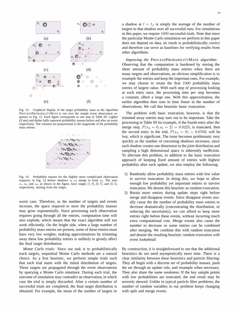
Fig. 13. Graphical display of the target probability mass as the algorithmPROCESSPROBABILITYMASS is run over the simple event observation se-quence in Fig. 12. Each figure corresponds to one step in Table III. Lighter(if any) and darker balls represent probability masses before and after an event,respectively. The volumes are proportional to the magnitude of the probabilitymass entries.

s 4

s 3

s 1

Fig. 14. Probability masses for the slightly more complicated observationsequence in Fig. 12 before shadows s1, s3 merge to form s5. The axess1, s3, and s4, as shown in the figure, have ranges [1, 9], [0, 7], and [0, 5],respectively, starting from the origin.

worst case. Therefore, as the number of targets and eventsincrease, the space required to store the probability massesmay grow exponentially. Since processing each observationrequires going through all the entries, computation time willalso explode, which means that the exact algorithm will notwork efficiently. On the bright side, when a large number ofprobability mass entries are present, some of these entries musthave very low weights; making approximations by trimmingaway these low probability entires is unlikely to greatly affectthe final target distribution.

Monte Carlo trials: Since our task is to probabilisticallytrack targets, sequential Monte Carlo methods are a naturalchoice. As a first heuristic, we perform simple trials suchthat each trial starts with the initial distribution of targets.These targets are propagated through the event observationsby querying a Monte Carlo simulator. During each trial, theoutcome of simulation may contradict an observation, in whichcase the trial is simply discarded. After a certain number ofsuccessful trials are completed, the final target distribution isobtained. For example, the mean of the number of targets in

a shadow at t = tf is simply the average of the number oftargets in that shadow over all successful runs. For simulationsin this paper, we require 1000 successful trials. Note that sincethe particular Monte Carlo simulation we perform in this paperdoes not depend on data, its result is probabilistically correctand therefore can serve as baselines for verifying results fromother algorithms.

Improving the PROCESSPROBABILITYMASS algorithm:Observing that the computation is burdened by storing thesheer amount of probability mass entries when there aremany targets and observations, an obvious simplification is toresample the entries and keep the important ones. For example,we may choose to retain the first 1000 probability massentries of largest value. With each step of processing lookingat each entry once, the processing time per step becomesa constant, albeit a large one. With this approximation, theearlier algorithm then runs in time linear in the number ofobservations. We call this heuristic basic truncation.

The problem with basic truncation, however, is that thetrimmed away entries may turn out to be important. Take theprocessing in Table III for example, if the fourth entry after themerge step, P (s4 = 0; s5 = 2) = 0.0225, is truncated, thenthe second entry in the end, P (s4 = 0) = 0.0769, will belost, which is significant. The issue becomes problematic veryquickly as the number of coexisting shadows increases, sinceeach shadow creates one dimension in the joint distribution andsampling a high dimensional space is inherently inefficient.To alleviate this problem, in addition to the basic truncationapproach of keeping fixed amount of entries with highestprobability after each update, we also employ the following:

1) Randomly allow probability mass entries with low valueto survive truncation. In doing this, we hope to allowenough low probability yet important entires to survivetruncation. We denote this heuristic as random truncation.

2) Retain more entries during update steps right beforemerge and disappear events. Since disappear events usu-ally cause the the number of probability mass entires todecrease dramatically (concentrating the distribution, orreducing the uncertainty), we can afford to keep moreentries right before these events, without incurring muchextra computational cost. Merge events also cause thenumber to decrease as some entries can be combinedafter merging. We combine this with random truncationand denote the resulting heuristic random truncation withevent lookahead.

By construction, it is straightforward to see that the additionalheuristics do not need asymptotically more time. There is aclear similarity between these heuristics and particle filtering:They all begin with a discrete set of probability masses, pushthe set through an update rule, and resample when necessary.They also share the same weakness: If the key sample pointswith low probabilities are truncated, the end result may beseverely skewed. Unlike in typical particle filter problems, thenumber of random variables in our problem keeps changingwith split and merge events.

15

F. Extensions

In subsection VI-A, assumptions 1) and 2) are made tosimplify the presentation of the probabilistic algorithms. Thefirst assumption is that component events are observed withouterror. Although component events can be observed with highaccuracy in many environments, it is not always the case.Sensor network is such an example: sensing range can be hardto know precisely. The extension to handle such uncertaintiesis relatively straightforward, at least in theory: all we need todo is to maintain a probability distribution over all possiblesequence of shadows consistent with the robot’s observations.Obtaining expectations of the number of targets in any shadowcan then be done by also calculating the expectation over allpossible sequences of shadows that contains the target shadow.The computation effort will certainly increase; resampling canalleviate the burden somewhat.

Various distinguishability assumptions can also be handled.Recall that in the nondeterministic formulation, two distin-guishability cases are investigated. When there are only teamswith single attributes, the approach from the nondeterministicsetting applies by simply carrying out one computation perteam. If the teams have multiple attributes (for example,the initial condition may be given as a joint distribution ofred and blue teams), a direct extension is performing onecomputation for each joint probability entries in the initialcondition. This is clearly more work and resampling may benecessary depending on the granularity of the initial targetdistribution. On the plus side, although we lose some accuracywith resampling (to save computation time), a richer class ofproblems can now be handled because any initial conditioncan be described as a joint probability distribution.

VII. SIMULATION RESULTS AND COMPLEXITY ANALYSIS

The simulation programs were developed adhering to theJava 1.6 language standard under the Eclipse environment. Thecomputations were performed on a workstation with an IntelCore 2 Quad processor running at 3.0 GHz. The JavaVM hasa maximum memory of 1.5GB. Although many parts of ouralgorithm can be easily parallelized, no multi-threading wasused in this implementation.

A. Nondeterministically moving targets

For the nondeterministic case, we implemented and testedthe algorithms for a single robot that moves in a simplyconnected polygonal region in R

2 using an omnidirectionalvisibility sensor. For such environment, the shadows arecompletely characterized by bitangents and inflections. Whenthe environment is known and the robot can localize itself,efficient 2D cell decomposition algorithms can be readilyapplied to obtain the sequence of shadows for each locationof the robot, allowing the shadows to be continuously tracked.This setup also enables us to construct an oracle (not availableto the algorithm) for distributing targets inside the free spaceto simulate their nondeterministic behavior. For max-flow,we implemented the O(V E2)-time Edmonds-Karp max-flowalgorithm [10], in which V and E are the numbers of verticesand edges in the flow graph, respectively.

(a) (b)

Fig. 15. Complicated examples that were used to test our approach. Thegiven robot trajectories are shown as green lines in the direction of the arrow.

For the environment in Figure 15(a), the trajectory generates85 component events. Our oracle randomly distributed 100targets in the free space as the component events occur. Thissetting yields a bipartite graph that has 41 vertices and 60edges. Calculating the lower and upper bounds for the 18 finalshadows for a single team took 0.1 seconds. The second freespace, shown in Figure 15(b), has 385 component events, 491total shadows, 124 vertices in the bipartite graph with 339edges. The example involves a million targets with 5 teams thatintersperse. The bounds on the 12 final shadow componentsfor all 5 teams were computed under one second.

The inputs to the base algorithm (single attribute, no FOVevents) are: 1) A sequence of n shadows, and 2) The initialcondition which takes the form of a pair of lower and upperbounds for each shadow at t = t0. In the worst case, thereare O(n) vertices and O(n2) edges in the bipartite graph.Edmonds-Karp max-flow then gives us O(n5) running timein the worst case. Applying a push-relabel algorithm withFIFO vertex selection rule will cut the running time to O(n3)[13]. Adding FOV events does not increase time complexityasymptotically, as discussed in subsection V-D. Adding partialdistinguishability, on the other hand, will introduce anotherinput parameter m, the number of teams, that contributeslinearly to time complexity. The typical worst case runningtime for the nondeterministic case is then O(n3m). Thenumber of targets in the system does not directly affect theperformance.

B. Probabilistic setup

1

8

a 13

time

76

17

12

9

4

2

5

11

20

10

3

19 18

1413

1615

a 20

a 16

Fig. 16. An event observation sequence with a total 20 shadows in its lifecycle. The FOV observations are not marked.

For the probabilistic case, we ran a simulation with theobservation sequence in Fig. 16. The sequence contains 14

16

component event observations. We also included 32 FOVevents scattered along the sequence, which are not markedin the figure. Shadows 1, 2, 3, 11, 13, 16, 20 are associatedwith 10, 7, 8, 9, 6, 9, 4 targets (with probability 1), respectively.For performance measures, we look at the time for one runof the algorithm to complete, as well as the expectation(mean and standard deviation for randomized methods) oftargets in individual shadows at the end (s17, s18, and s19).When we randomly pick entries to keep, the time result isaveraged over 10 runs and the accuracy is given in the formof mean and standard deviation. In our implementation, wealso make the following choices: 1) for random truncation,the entries are kept based on its probability multiplied witha random number in (0, 1), 2) for event lookahead, we willnot truncate the entries if there is a disappear event withinthe next four events or a merge event within the next twoevents. The outcome is summarized in Table IV. The heuristicsbasic truncation, random truncation, and random truncationwith event lookahead are shortened as TR, RT, and RT-LA,respectively. The number following the method is the numberof entries kept. By frequent failure, we mean that more than1/3 of the times the heuristic fails to give a valid result. Theseare indicative of minimum number of entries needed for themethod to work.

TABLE IV

heuristic s17 s18 s19 t(s)none, precise 11.12 5.84 5.60 329.5TR-10000 failureTR-20000 10.67 4.85 5.33 6.1TR-50000 11.00 5.38 5.52 15.5TR-100000 10.96 5.59 5.53 29.4TR-200000 11.06 5.73 5.56 61.4RT-10000 frequent failureRT-20000 11.38(0.20) 5.31(0.23) 5.67(0.20) 6.1RT-50000 11.16(0.02) 5.36(0.03) 5.64(0.02) 14.6RT-100000 11.03(0.01) 5.62(0.01) 5.56(0.01) 28.3RT-LA-2000 frequent failureRT-LA-5000 11.32(1.30) 6.54(1.46) 5.28(1.28) 2.0RT-LA-10000 11.17(0.56) 5.87(0.91) 5.02(0.48) 4.2RT-LA-20000 11.62(0.26) 5.30(0.18) 5.57(0.16) 8.3RT-LA-50000 11.32(0.01) 5.51(0.01) 5.60(0.01) 17.7Monte Carlo 11.16 5.58 5.57 42.1

The result shows that when no heuristic is used, the algo-rithm takes much more time to finish. This is not surprisingsince the time complexity is induced by the space requirementfor storing the probability mass entries. On the other hand, allof the truncation heuristics work reasonably well, with the ran-domized truncation plus event lookahead greatly reduces thenumber of entries to retain. The RT-LA-50000 run compareswell with the TR-100000 run on accuracy, but uses one thirdless time. We expect the advantage to become more obviousas more targets are present in the system.

For a second test, we change the number of targets inshadows 1, 2, 3, 13, 16, 20 to 25, 22, 23, 8, 15, 9, while leavingother observations unchanged. With the increased number oftargets, the basic algorithm runs out of memory after 10minutes, before the third split is completed. At the peakof its memory usage during the failed run, there are morethan 2 × 107 probability mass entries. On the other hand,

the randomized methods do not have this problem: Both RT-100000 RT-LA-50000 yield good results compared to MonteCarlo trials, with similar running time. The result is sum-marized in Table V. Comprehensive performance analysis of

TABLE V

Heuristic s17 s18 s19 t(s)none, exact out of memory after 10 minsMonte Carlo 18.26 22.25 11.85 43.2RT-100000 17.78(0.03) 21.83(0.03) 12.34(0.02) 66.3RT-LA-50000 18.24(0.08) 21.99(0.07) 12.57(0.07) 40.6

probabilistic algorithm is hard since the performance dependson external factors such as the implementation of the specificsplit rule, random number generator, and so on. Nevertheless,for completeness, we discuss the performance at a higherlevel. To avoid the issue of external factors, we assumethat at each step, each probability mass takes constant timeto process. Unlike the nondeterministic case, running timeof the PROCESSPROBABILITYMASS algorithm may dependheavily on the number of targets in the system via the splitrule. If there are n split events with an average number oftargets in the originating shadow being p and also nf FOVevents, with the reasonable additional assumption that merge,appear, and disappear events are on the same order as splitevents, the PROCESSPROBABILITYMASS algorithm can taketime O(pn3nf ). The running time of the resampling basedalgorithms has a big constant depending on the number ofentries to keep, but otherwise depends only linearly on thenumber of critical events.

VIII. CONCLUSION

In conclusion, we have formulated and solved, at a verygeneral level, the problem of tracking targets moving in andout of the FOV of moving sensors. The resulting filters maybe applied in numerous settings, such as pursuit-evasion,target enumeration, and situational awareness. When targetsmove nondeterministically, a combinatorial filter is proposedfor the tracking task: We show that the naturally emerginginteger linear programming problem is in fact solvable inpolynomial time and provide an efficient max-flow basedsolution for it. For the probabilistic filtering problem in whichtargets move probabilistically and sensors are not reliable,we give both exact and efficient algorithms that handle theseveral possible scenarios depending on the number of targetsand observations in a system. In solving the more general,probabilistic version of the tracking problem, a clear link isalso established between combinatorial filtering and Bayesianfiltering methods: The final target distribution is in essenceassociating the combinatorial solution, a polytope structure,with appropriate probabilities. Viewing it from another angle,the probabilistic shadow I-space extends naturally from itsnondeterministic counterpart, by merely adding dimensions torecord probabilities.

Acknowledgments: This work was supported in part byNSF grants 0904501 (IIS Robotics) and 1035345 (Cyberphys-ical Systems), DARPA SToMP grant HR0011-05-1-0008, andMURI/ONR grant N00014-09-1-1052.

17

REFERENCES

[1] S. Alexander, R. Bishop, and R. Ghrist. Pursuit and evasion in non-convex domains of arbitrary dimension. In G. S. Sukhatme, S. Schaal,W. Burgard, and D. Fox, editors, Robotics: Science and Systems II. MITPress, Cambridge, MA, 2007.

[2] L. Alonso, A. S. Goldstein, and E. M. Reingold. Lion and man: Upperand lower bounds. ORSA Journal of Computing, 4(4):447–452, 1992.

[3] Y. Baryshnikov and R. Ghrist. Target enumeration via euler characteris-tic integrals. SIAM Journal of Applied Mathematics, 70(4):825, August2009.

[4] P. E. Berry, C. Pontecorvo, and D. A. B. Fogg. Optimal search, locationand tracking of surface maritime targets by a constellation of surveillancesatellites. Technical report, DSTO Information Sciences Laboratory,Edingburgh, SA, 2003.

[5] S. D. Bopardikar, F. Bullo, and J. P. Hespanha. On discrete-time pursuit-evasion games with sensing limitations. IEEE Transactions on Robotics,24(6):1429–1439, 2008.

[6] P. Bose, A. Lubiv, and J. I. Munro. Efficient visibility queries in simplepolygons. In Proceedings Canadian Conference on ComputationalGeometry, pages 23–28, 1992.

[7] F. Bourgault, T. Furukawa, and H.F. Durrant-Whyte. Coordinateddecentralized search for a lost target in a bayesian world. In Proceedings2003 IEEE/RSJ International Conference on Intelligent Robots andSystems, pages 48 – 53 vol.1, 2003.

[8] W.-P. Chin and S. Ntafos. Optimum watchman routes. InformationProcessing Letters, 28:39–44, 1988.

[9] W.-P. Chin and S. Ntafos. Optimum watchman routes in simplepolygons. Discrete and Computational Geometry, 6:9–31, 1991.

[10] J. Edmonds and R. M. Karp. Theoretical improvements in algorithmicefficiency for network flow problems. J. ACM, 19(2):248–264, 1972.

[11] B. P. Gerkey, S. Thrun, and G. Gordon. Visibility-based pursuit-evasionwith limited field of view. International Journal of Robotics Research,25(4):299–322, 2006.

[12] B. Gfeller, M. Mihalak, S. Suri, E. Vicari, and P. Widmayer. Countingtargets with mobile sensors in an unknown environment. In ALGOSEN-SORS, July 2007.

[13] A. V. Goldberg and R. E. Tarjan. A new approach to the maximum flowproblem. In STOC ’86: Proceedings of the eighteenth annual ACMsymposium on Theory of computing, pages 136–146, New York, NY,USA, 1986. ACM.

[14] L. J. Guibas, J.-C. Latombe, S. M. LaValle, D. Lin, and R. Motwani.Visibility-based pursuit-evasion in a polygonal environment. Interna-tional Journal of Computational Geometry and Applications, 9(5):471–494, 1999.

[15] O. Hajek. Pursuit Games. Academic, New York, 1975.[16] Y. Ho, A. E. Bryson, and S. Baron. Differential games and optimal

pursuit-evasion strategies. IEEE Transactions on Automatic Control,10(4):385–389, 1965.

[17] R. Isaacs. Differential Games. Wiley, New York, 1965.[18] V. Isler, S. Kannan, , and S. Khanna. Randomized pursuit-evasion in a

polygonal environment. IEEE Transactions on Robotics, 5(21):864–875,2005.

[19] R. E. Kalman. A new approach to linear filtering and predictionproblems. Transactions of the ASME, Journal of Basic Engineering,82:35–45, 1960.

[20] T. Kameda, M. Yamashita, and I. Suzuki. On-line polygon search bya seven-state boundary 1-searcher. IEEE Transactions on Robotics,22:446–460, Jun 2006.

[21] S. Kopparty and C. V. Ravishankar. A framework for pursuit evasiongames in Rn. Information Processing Letters, 96(3):114–122, 2005.

[22] S. M. LaValle. Planning Algorithms. Cambridge University Press,Cambridge, U.K., 2006. Also available at http://planning.cs.uiuc.edu/.

[23] S. M. LaValle and J. Hinrichsen. Visibility-based pursuit-evasion: Thecase of curved environments. IEEE Transactions on Robotics andAutomation, 17(2):196–201, April 2001.

[24] S. M. LaValle, D. Lin, L. J. Guibas, J.-C. Latombe, and R. Motwani.Finding an unpredictable target in a workspace with obstacles. In Pro-ceedings IEEE International Conference on Robotics and Automation,pages 737–742, 1997.

[25] S.-H. Lim, T. Furukawa, G. Dissanayake, and H. F. Durrant-Whyte. Atime-optimal control strategy for pursuit-evasion games problems. InProceedings IEEE International Conference on Robotics & Automation,2004.

[26] R. Mahler. Objective functions for bayesian control-theoretic sensormanagement, ıı: Mhc-like approximation. In S. Butenko, R. Murphey,and P. Paralos, editors, New Developments in Cooperative Control and

Optimization, pages 273–316, Norwell, MA, 2003. Kluwer AcademicPublishers.

[27] J. O’Rourke. Art Gallery Theorems and Algorithms. Oxford UniversityPress, New York, 1987.

[28] J. O’Rourke. Visibility. In J. E. Goodman and J. O’Rourke, editors,Handbook of Discrete and Computational Geometry, 2nd Ed., pages643–663. Chapman and Hall/CRC Press, New York, 2004.

[29] M. Pachter. Simple motion pursuit-evasion differential games. InMediterranean Conference on Control and Automation, Lisbon, Por-tugal, July 2002.

[30] C. H. Papadimitriou and K. J. Steiglitz. Combinatorial Optimization:Algorithms and Complexity. Prentice Hall, Englewood Cliffs, NJ, 1982.

[31] S.-M. Park, J.-H. Lee, and K.-Y. Chwa. Visibility-based pursuit-evasionin a polygonal region by a searcher. Technical Report CS/TR-2001-161,Dept. of Computer Science, KAIST, Seoul, South Korea, January 2001.

[32] T. D. Parsons. Pursuit-evasion in a graph. In Y. Alavi and D. R. Lick,editors, Theory and Application of Graphs, pages 426–441. Springer-Verlag, Berlin, 1976.

[33] S. Petitjean, D. Kriegman, and J. Ponce. Computing exact aspect graphsof curved objects: algebraic surfaces. International Journal of ComputerVision, 9:231–255, Dec 1992.

[34] M. Pocchiola and G. Vegter. The visibility complex. InternationalJournal Computational Geometry & Applications, 6(3):279–308, 1996.

[35] S. Sachs, S. Rajko, and S. M. LaValle. Visibility-based pursuit-evasionin an unknown planar environment. International Journal of RoboticsResearch, 23(1):3–26, January 2004.

[36] A. Schrijver. Combinatorial Optimization. Springer-Verlag, 2003.[37] J. Sgall. A solution of david gales lion and man problem. Theoretical

Computational Science, 259(1-2):663–670, 2001.[38] T. Shermer. Recent results in art galleries. Proceedings of the IEEE,

80(9):1384–1399, September 1992.[39] B. Simov, G. Slutzki, and S. M. LaValle. Pursuit-evasion using beam

detection. In Proceedings IEEE International Conference on Roboticsand Automation, 2000.

[40] J. Singh, R. Kumar, U. Madhow, S. Suri, and R. Cagley. Trackingmultiple targets using binary proximity sensors. In Proc. InformationProcessing in Sensor Networks, 2007.

[41] L. D. Stone. Theory of Optimal Search. Academic Press, New York,NY, 1975.

[42] I. Suzuki and M. Yamashita. Searching for a mobile intruder in apolygonal region. SIAM Journal on Computing, 21(5):863–888, October1992.

[43] B. Tovar, F. Cohen, and S. M. LaValle. Sensor beams, obstacles, andpossible paths. In Proceedings Workshop on Algorithmic Foundationsof Robotics, 2008.

[44] B. Tovar and S. M. LaValle. Visibility-based pursuit-evasion withbounded speed. International Journal of Robotics Research, 2007. Underreview (invited submission from WAFR 2006).

[45] B. Tovar, R Murrieta, and S. M. LaValle. Distance-optimal navigation inan unknown environment without sensing distances. IEEE Transactionson Robotics, 23(3):506–518, June 2007.

[46] V. Turetsky. Upper bounds of the pursuer control based on a linear-quadratic differential game. Journal of Optimization Theory andApplications, 121(1):163–191, April 2004.

[47] R. Vidal, O. Shakernia, H. J. Kim, D. H. Shim, and S. Sastry. Prob-abalistic pursuit-evasion games: Theory, implementation, and experi-mental evaluation. IEEE Transactions on Robotics and Automation,18(5):662669, 2002.

[48] C.-C. Wang, C. Thorpe, S. Thrun, M. Hebert, and H. Durrant-Whyte.Simultaneous localization, mapping and moving object tracking. Inter-national Journal of Robotics Research, 26(9):889–916, 2007.

[49] I. Yan and G. L. Blankenship. Numerical methods in search pathplanning. In Proceedings of the 27th IEEE Conference on Decisionand Control, pages 1563 –1569 vol.2, 1988.

[50] D. B. Yang, H. H. Gonzalez-Banos, and L. J. Guibas. Counting peoplein crowds with a real-time network of simple image sensors. In Proc.IEEE International Conference on Computer Vision, volume 1, pages122– 129, 2003.

[51] J. Yu and S. M. LaValle. Tracking hidden agents through shadowinformation spaces. In Proceedings IEEE International Conference onRobotics and Automation, 2008.

[52] J. Yu and S. M. LaValle. Probabilistic shadow information spaces. InProceedings IEEE International Conference on Robotics and Automa-tion, 2010.