1

Shadow prices of air pollutants in Czech industries: A convex nonparametric least squares approach

Lukáš Rečka*,+ Milan Ščasný*

Abstract

The paper estimates the shadow prices of SO2 emissions for 36 Czech industry sectors during the

period 2000-2008. A convex nonparametric least squares quadratic optimization formulated by

Mekaroonreung & Johnson (2012) is applied to measure technical efficiency and to jointly estimate the

shadow prices of SO2 emissions. The weighted average shadow price ranges between 360€ and 1,316€

per ton of SO2 and it declines over time. These values are in line with other estimates of SO2 shadow

price and marginal abatement cost estimated for the Czech Republic. Since the estimated shadow

prices of emissions can be interpreted as marginal abatement cost, the ExternE method is applied to

compare them with the marginal environmental external costs that are attributable to SO2 emissions

released by the industry sector. We conclude that current regulation is far from the economic optimum,

since the estimated SO2 shadow prices are much lower than corresponding marginal damage costs: in

some sectors the shadow prices are even one order of magnitude smaller than the external costs. Since

current market-based instruments have internalised the external costs only partly, these instruments

have been ineffective and economically sub-optimal.

Keywords: Shadow price; abatement cost; externality; nonparametric regression; SO2

JEL Code: C14, Q53, Q58

* Environment Center, Charles University in Prague, José Martího 407/2, 162 00 Prague, Czech Republic + Institute of Economic Studies, Faculty of Social Sciences, Charles University in Prague, Opletalova 26, 110 00 Prague,

Czech Republic

2

1 INTRODUCTION

The Czech Republic, with a 28% of GDP represented by industry, belongs among the most

industrialized countries in the European Union (Eurostat, 20115). Although the air quality in the Czech

Republic has significantly improved as a result of stricter air quality control during the transition

period in 1990’s and the implementation of environmental acquis communitaire of the European

Union in the following decade (Ščasný & Máca, 2009), sustainable energy (Olabi, 2014) is far away

and further airborne emission reduction (Ščasný et al. 2009) and energy savings are desirable. In

reality, however, since the end of 1990’s the rate of emission reduction has slowed down significantly

(EEA, 2014). The aim of our paper is therefore to identify sectors with the highest economic potential

for reduction of sulphurous emissions1 in the Czech Republic, measured through the shadow price of

SO2 across the industry sectors. We also aim to compare the implicit price of SO2 emissions with the

magnitude of damage caused by these emissions and with the current level of market-based

instruments which should internalise these external costs.

We contribute to the literature by estimating shadow prices of SO2 emissions emitted by 36 industrial

sectors in a post-transition European country, the Czech Republic, during the years 2000 to 2008,

supplementing our previous study based on ODF method and aimed at the Czech power sector (Rečka

& Ščasný, 2011). In this paper, we specifically follow the Mekaroonreung & Johnson (2012) study and

apply Convex Nonparametric Least Squares quadratic optimization to analyse technical efficiency

jointly with emission shadow price estimation. Then we apply the impact pathway analysis embedded

in the ExternE method (Preiss, Friedrich, & Klotz, 2008) to quantify the environmental external costs

attributable to SO2 emissions. Lastly, the shadow prices (i.e. the marginal abatement costs) are

compared with corresponding external costs to draw policy-relevant conclusions.

Our findings indicate a significant potential for SO2 emission reduction in the sectors with high SO2

emission production. The weighted average of estimated shadow prices is at the value of 834€ per ton

of SO2 and has a decreasing trend from more than 1100€ 2000 to less than 500€ in 2008. The rest of

the paper is organized as follows: section 2 describes our method, i.e. the CNLS quadratic optimization

problem applied for the inefficiency estimation, and how our approach derives the shadow prices and

the external cost. Section 3 describes the data used, and Section 4 presents the results. The final section

draws concluding remarks.

2 LITERATURE REVIEW

Färe et al. (1990) provided the first estimates of shadow prices of production factors based on a

frontier approach. Färe and Grosskopf (1993) were then the first who applied Shephard’s (1970)

concept of weak disposability between desirable and undesirable outputs on distance function with the

translog functional form in order to estimate the shadow price of four air pollutants released from pulp

and paper mills in Michigan and Wisconsin, USA. Since translog or similar functional forms of the

distance function are differentiable, this parametric approach was applied in many other studies,

mostly in the USA and Asia (e.g. Bauman, Lee, & Seeley, 2008; Coggins & Swinton, 1996; Gupta,

2006; Hailu & Veeman, 2000; Kwon & Yun, 1999; John R. Swinton, 1998) thanks to the fact that

functions are differentiable everywhere. On the other hand, if the functional form is misspecified, the

parametric approach can yield biased estimates.

1 Sulphurous emissions are measured as SOX (mixture of SO2/SO3) and are expressed in SO2 equivalents.

3

Alternatively, Boyd et al. (1996) used a nonparametric specification of directional distance function to

estimate the marginal abatement cost (MAC) of SO2 on a sample of 62 US power plants. Lee et al.

(2002) extended the nonparametric direction distance function approach to control also for the

inefficiency in production process. For these purposes, Lee et al. (2002) define an efficiency rule as

𝜎𝑔 = 𝜎𝑔(𝜆), 𝜎𝑏 = 𝜎𝑏(𝜆) , where 𝜎𝑔 and 𝜎𝑏 are called inefficiency factors and 𝜆 is a parameter relating

𝜎𝑔 to 𝜎𝑏. The efficiency rule maps a point (𝑦, 𝑏) ∈ 𝑃(𝑥) to corresponding (𝑦∗, 𝑏∗) on the boundary

𝑃(𝑥) in a way that 𝜎𝑔(𝜆)𝑦 = 𝑦∗, 𝜎𝑏(𝜆)𝑏 = 𝑏∗, where y, b and x denotes the vectors of desirable

outputs, undesirable outputs, and inputs, respectively. Furthermore they defined an efficiency path and

iso-efficiency path as follows: 𝐸𝑃(𝑦∗, 𝑏∗) = [(𝑦, 𝑏) ∈ 𝑃(𝑥): 𝜎𝑔(𝜆)𝑦 = 𝑦∗, 𝜎𝑏(𝜆)𝑏 = 𝑏∗

and 𝐼𝐸𝑃(𝑦0, 𝑏0) = [(𝑦, 𝑏) ∈ 𝑃(𝑥): 𝐷(𝑥, 𝜎𝑔0𝑦, 𝜎𝑏

0𝑏) = 1], respectively. Following Kumbhakar et al.

(n.d.), they estimate the direction distance function with the elements 𝜎𝑔𝑦 𝑎𝑛𝑑 𝜎𝑏𝑏, when the

directional vector 𝑔 = (𝑏, 𝑦) is calculated “by utilizing the annual abatement schedules of pollutants

and the production plans of good output as proxy variables for 𝑏 and 𝑦, respectively” (J.-D. Lee et al.,

2002, p. 371). Using this nonparametric approach and controlling for inefficiency, the shadow price of

SOx, NOx and TSP is estimated for the electric power industry in Korea during the period of 1990-

1995 in a sample of 43 power plants. They found the average shadow prices “are approximately 10%

lower than those calculated under the assumption of full efficiency”(J.-D. Lee et al., 2002, p. 365).

Still this deterministic nonparametric approach cannot capture statistical noise – thus the data must be

without error and the production model specified without omitting any inputs or outputs

(Mekaroonreung & Johnson, 2012) – and is more sensitive to outliers than parametric methods.

More recent nonparametric approaches, such as Convex Nonparametric Least Squares, (CNLS) as

developed by Kuosmanen & Johnson (2008), deal with the two above drawbacks, i.e. sensitivity to

outliers and exclusion of statistical inference. Kuosmanen & Kortelainen (2012) introduce a two-stage

Stochastic Non-parametric Envelopment method (StoNED) that combines a nonparametric data

envelopment analysis with a stochastic frontier analysis to decompose statistical noise and

inefficiency. Mekaroonreung & Johnson (2012) extend the StoNED method by applying CNLS

quadratic optimization to estimate a frontier production function and the shadow prices for SO2 and

NOx emitted by US coal power plants.

The studies that estimate the shadow price of emissions can be also differentiated according to level of

data disaggregation or environmental domain that is examined. Regarding the former dimension, most

of the studies are based on firm level data focusing on an individual sector (e.g. Färe et al., 1993; Färe,

Grosskopf, Noh, & Weber, 2005; Mekaroonreung & Johnson 2012; Park & Lim 2009), whereas there

are some studies that estimated the shadow price of emissions at country level (e.g. Wu, Chen, & Liou

(2013) or Salnykov & Zelenyuk (2004)). To our knowledge, only Peng et al. (2012) have estimated the

shadow prices of pollutants using sector-level data. Considering the latter dimension of studies, most

of the literature has dealt with airborne pollution and GHG (e.g. Boyd et al., 1996; Färe et al., 2005;

John R. Swinton, 1998), while water pollution and other environmental burdens have been analysed

less often (e.g. Färe et al., 1993; Hailu & Veeman, 2000; Marklund, 2003).

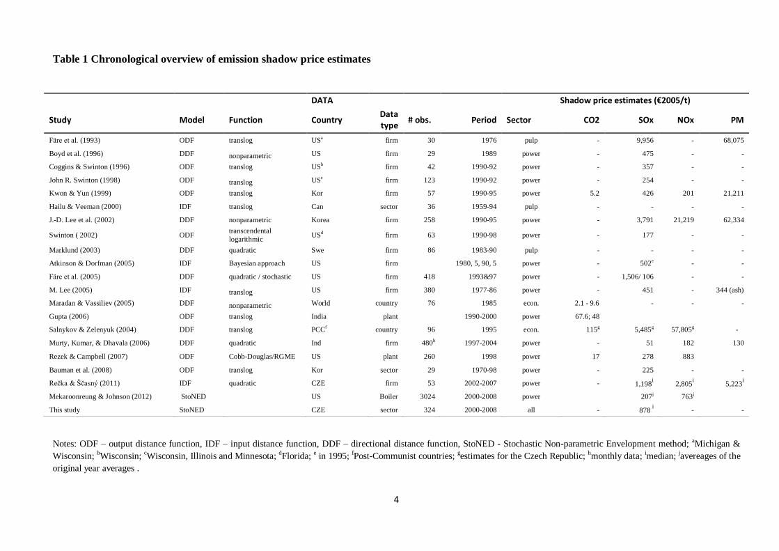
Chyba! Nenalezen zdroj odkazů. provides a chronological overview of the shadow price estimates for air

emissions.

4

Table 1 Chronological overview of emission shadow price estimates

Notes: ODF – output distance function, IDF – input distance function, DDF – directional distance function, StoNED - Stochastic Non-parametric Envelopment method; aMichigan &

Wisconsin; bWisconsin; cWisconsin, Illinois and Minnesota; dFlorida; e in 1995; fPost-Communist countries; gestimates for the Czech Republic; hmonthly data; imedian; javereages of the

original year averages .

DATA Shadow price estimates (€2005/t)

Study Model Function Country Data type

# obs. Period Sector CO2 SOx NOx PM

Färe et al. (1993) ODF translog USa firm 30 1976 pulp - 9,956 - 68,075

Boyd et al. (1996) DDF nonparametric US firm 29 1989 power - 475 - -

Coggins & Swinton (1996) ODF translog USb

firm 42 1990-92 power - 357 - -

John R. Swinton (1998) ODF translog USc firm 123 1990-92 power - 254 - -

Kwon & Yun (1999) ODF translog Kor firm 57 1990-95 power 5.2 426 201 21,211

Hailu & Veeman (2000) IDF translog Can sector 36 1959-94 pulp - - - -

J.-D. Lee et al. (2002) DDF nonparametric Korea firm 258 1990-95 power - 3,791 21,219 62,334

Swinton ( 2002) ODF transcendental

logarithmic US

d firm 63 1990-98 power - 177 - -

Marklund (2003) DDF quadratic Swe firm 86 1983-90 pulp - - - -

Atkinson & Dorfman (2005) IDF Bayesian approach US firm

1980, 5, 90, 5 power - 502e - -

Färe et al. (2005) DDF quadratic / stochastic US firm 418 1993&97 power - 1,506/ 106 - -

M. Lee (2005) IDF translog US firm 380 1977-86 power - 451 - 344 (ash)

Maradan & Vassiliev (2005) DDF nonparametric World country 76 1985 econ. 2.1 - 9.6 - - -

Gupta (2006) ODF translog India plant

1990-2000 power 67.6; 48

Salnykov & Zelenyuk (2004) DDF translog PCCf country 96 1995 econ. 115

g 5,485

g 57,805

g -

Murty, Kumar, & Dhavala (2006) DDF quadratic Ind firm 480h 1997-2004 power - 51 182 130

Rezek & Campbell (2007) ODF Cobb-Douglas/RGME US plant 260 1998 power 17 278 883

Bauman et al. (2008) ODF translog Kor sector 29 1970-98 power - 225 - -

Rečka & Ščasný (2011) IDF quadratic CZE firm 53 2002-2007 power - 1,198i 2,805

i 5,223

i

Mekaroonreung & Johnson (2012) StoNED

US Boiler 3024 2000-2008 power 207j

763j

This study StoNED

CZE sector 324 2000-2008 all - 878 i - -

5

3 METHODS

Following Mekaroonreung & Johnson (2012) and Shephard (1970) we define the production

possibility set. For each industry 𝑖 = 1, … , 𝑛 let 𝑥 ∈ 𝑅+𝑀 is a vector of inputs, 𝑦 ∈ 𝑅+

𝑆 is vector of good

outputs and 𝑏 ∈ 𝑅+𝐽 is a vector of bad outputs. The basic characterization of the polluting production

technology is the technology set 𝑇 of all feasible input-output combination: 𝑇 = [(𝑥, 𝑦, 𝑏) ∶𝑥 can produce (𝑦, 𝑏) ]. 𝑇 is convex and there are variable returns to scale.

The production technology satisfies the following assumption, orginaly proposed by Shephard (1970):

1. Free disposibility of inputs:

if (𝑥, 𝑦, 𝑏) ∈ 𝑇and �́� ≥ 𝑥, then (�́�, 𝑦, 𝑏) ∈ 𝑇.

2. Free disposability of good outputs:

if (𝑥, 𝑦, 𝑏) ∈ 𝑇 and 𝑦0 ≤ 𝑦 then (𝑥, 𝑦0, 𝑏) ∈ 𝑇.

3. Weak disposibility between good and bad outputs: if (𝑥, 𝑦, 𝑏) ∈ 𝑇 and 0 ≤ 𝜃 ≤ 1 then

(𝑥, 𝜃𝑦, 𝜃𝑏) ∈ 𝑇.

The variable returns to scale weakly disposable production possibility set 𝑇 can then be rewritted as

(Mekaroonreung & Johnson (2012) ):

𝑇 = {(𝑥, 𝑦, 𝑏) ∈ 𝑅+𝑀+𝑆+𝐽|𝑥 ≥ ∑(𝜆𝑖 + 𝜇𝑖)𝑥𝑖 ; 𝑦 ≤ ∑ 𝜆𝑖𝑦𝑖

𝑛

𝑖=1

;

𝑛

𝑖=1

𝑏 ≥ ∑ 𝜆𝑖𝑏𝑖

𝑛

𝑖=1

; ∑(𝜆𝑖 + 𝜇𝑖)

𝑛

𝑖=1

= 1, 𝜆𝑖, 𝜇𝑖 ≥ 0}

(1)

where 𝜆𝑖 allows the convex combination of observed industries and 𝜇𝑖 allows to scale down both good

outputs and bad ouputs while maintaining the level of inputs. Note that the inequality in bad output

constrains implies a negative shadow price on additional pollution which satisfies the economic

intuition incurring certain costs in production (Mekaroonreung & Johnson, 2012).

We apply the CNLS technique with composite disturbance term considering a single output production

function with a multiplicative disturbance term:

𝑦𝑖 = 𝑓(𝑥𝑖, 𝑏𝑖) exp(𝜖𝑖) ∀𝑖 = 1, … , 𝑛 (2)

where 𝑓(𝑥𝑖, 𝑏𝑖) satisfies continuity, monotonicity, concavity and weak disposability; 𝜖𝑖 is disturbance

term and the bad outputs are treated as independent variables, as in Cropper & Oates (1992).

Applying the log transformation to (2) we obtain (3):

𝜖𝑖 = ln(𝑦𝑖) − ln(𝑓(𝑥𝑖, 𝑏𝑖)) (3)

Following Mekaroonreung & Johnson (2012) we assume statistical noise in the data and therefore the

disturbance term can be written as:

𝜖𝑖 = 𝑣𝑖 − 𝑢𝑖 ∀𝑖 = 1, … , 𝑛 (4)

where 𝑣𝑖 is a random noise component.

6

Because – as Kuosmanen & Kortelainen (2012) point out – the composite disturbance term in (4)

violates the Gauss-Markov properties that 𝐸(𝜖𝑖) = 𝐸(−𝑢𝑖) = −𝜇 < 0, the composite disturbance term

is modified and the multiplicative disturbance production model 𝑦𝑖 = 𝑓(𝑥𝑖, 𝑏𝑖)exp (𝜖𝑖) is written as in

Mekaroonreung & Johnson (2012):

ln(𝑦𝑖) = [ln(𝑓(𝑥𝑖, 𝑏𝑖 )) − 𝜇] + [𝜖𝑖 + 𝜇] = ln(𝑔(𝑥𝑖, 𝑏𝑖 )) + 𝜈𝑖 ∀𝑖 = 1, … , 𝑛 (5)

where 𝜈𝑖 = 𝜖𝑖 + 𝜇 is the modified composite disturbance term and 𝐸(𝜈𝑖) = 𝐸(𝜖𝑖 + 𝜇)=0. The CNLS

problem is then defined as follows:

min𝛼,𝑤,𝑐,𝜈

∑ 𝜈𝑖2

𝑛

𝑖=1

s.t. 𝜈𝑖 = ln(𝑦𝑖) − ln(𝛼𝑖 + 𝑤𝑖′𝑥𝑖 − 𝑐𝑖

′𝑏𝑖) ∀𝑖 = 1, … , 𝑛

𝛼𝑖 + 𝑤𝑖′𝑥𝑖 − 𝑐𝑖

′𝑏𝑖 ≤ 𝛼ℎ + 𝑤ℎ′ 𝑥𝑖 − 𝑐ℎ

′ 𝑏𝑖 ∀𝑖, ℎ = 1, … , 𝑛

𝛼𝑖 + 𝑤𝑖′𝑥ℎ ≥ 0 ∀𝑖, ℎ = 1, … , 𝑛

𝑤𝑖 , 𝑐𝑖 ≥ 0 ∀𝑖 = 1, … , 𝑛

(6)

where 𝑤𝑖 = (𝑤𝑖1, … , 𝑤𝑖𝑀) and 𝑐𝑖 = (𝑐𝑖1, … , 𝑐𝑖𝐽) are marginal products of good output and bad output,

respectively.

The technical efficiency and statistical noise components are separated using the estimated modified

CNLS residuals �̂�𝑖 from (6) in the second stage of CNLS. Assuming technical efficiency is

independent and identically distributed (i.i.d.) and has a half normal distribution and the statistical

noise is i.i.d. and normally distributed, 𝑢𝑖~|𝑁(0, 𝜎𝑢2)| and 𝑣𝑖~𝑁(0, 𝜎𝑢

2), the method of moments

(Aigner, Lovell, & Schmidt, 1977) is applied as in Mekaroonreung & Johnson (2012):

�̂�𝑢 = √�̂�3

(2

𝜋)(1−

4

𝜋)

3 and �̂�𝑣 = √�̂�2 − (

𝜋−2

𝜋) �̂�𝑢

2 (7)

where �̂�2 =1

𝑛∑ (�̂�𝑖 − �̂�(𝜈𝑖))

2𝑛𝑖=1 and �̂�3 = ∑ (�̂�𝑖 − �̂�(𝜈𝑖))

3𝑛𝑖=1 .

The average production function 𝑔(𝑥𝑖, 𝑏𝑖) is obtained from the CNLS problem (6) and it is multiplied

by the expected technical efficiency to estimate the production function:

ln(�̂�(𝑥𝑖, 𝑏𝑖)) = [ln (𝑓(𝑥𝑖, 𝑏𝑖)) − �̂�] = ln(𝑓(𝑥𝑖, 𝑏𝑖) − 𝑒𝑥𝑝(−�̂�)), thus

𝑓(𝑥𝑖, 𝑏𝑖) = �̂�(𝑥𝑖, 𝑏𝑖)exp (�̂�) (8)

where �̂� = �̂�𝑢√2

𝜋.

Jondrow et al. (1982) decomposition can be applied to estimate industry specific inefficiency based on

�̂�𝑢 and �̂�𝑣:

�̂�(𝑢𝑖|𝜖�̂�) = −𝜖�̂��̂�𝑢

2

�̂�𝑢2 + �̂�𝜈

2 +�̂�𝑢

2�̂�𝜈2

�̂�𝑢2 + �̂�𝜈

2 [𝜙(𝜖�̂� �̂�𝜈

2⁄ )

1 − Φ(𝜖�̂� �̂�𝜈2⁄ )

] (9)

where 𝜖�̂� = �̂�𝑖 − �̂�, 𝜙 is the standard normal density function and Φ is the standard normal cumulative

distribution.

7

3.1 Shadow Price Of Emissions

Assuming profit-maximizing behaviour for all firms in each industry, the profit maximization problem

for a production process with outputs and pollutants (i.e. bad outputs) is the following:

𝜋(𝑝𝑦, 𝑝𝑏 , 𝑝𝑥) = max𝑦,𝑏,𝑥

𝑝𝑦′ 𝑦 − 𝑝𝑏

′ 𝑏 − 𝑝𝑥′ x

s.t. (𝐹((𝑥, 𝑏, 𝑦)) = 0) (10)

where 𝑝𝑦 = (𝑝𝑦1, … , 𝑝𝑦𝑆

),𝑝𝑏 = (𝑝𝑏1, … , 𝑝𝑏𝐽

), 𝑝𝑥 = (𝑝𝑥1, … , 𝑝𝑥𝑀

) are the price vectors of outputs,

pollutants and inputs, respectively. As in Mekaroonreung & Johnson (2012) 𝐹(𝑥, 𝑏, 𝑦) is the

transformation function corresponding to a multi-output production function and since the shadow

price of pollutants are our focus, the constrain 𝐹(𝑥, 𝑏, 𝑦) = 0 is imposed in order to consider only the

production possibility set. Applying the method of Lagrangian multipliers to (7) and following Färe et

al. (1993), the relative shadow price of pollutants for industry 𝑖 are estimated as follows:

𝑝𝑏𝑖𝑗= 𝑝𝑦𝑖

𝜕𝑓(𝑥𝑖, 𝑏𝑖)

𝜕𝑏𝑖𝑗 (11)

where 𝑝𝑦𝑖is price of and output of industry 𝑖. Since we use gross value added as a proxy of the

industry’s output, 𝑝𝑦𝑖= 1. By solving the CNLS problem (6) we estimate first the average weak

disposability production function �̂�(𝑥𝑖, 𝑏𝑖) and second we calculate the estimated expected inefficiency

components �̂�. The relative shadow price of pollutants for each industry is obtained as 𝜕�̂�(𝑥𝑖,𝑏𝑖)

𝜕𝑏𝑖𝑗exp(�̂�) = 𝑐�̂�𝑗exp (�̂�), where the variable 𝑐�̂�𝑗 ∈ 𝑐�̂� = (𝑐�̂�1, … , 𝑐�̂�𝐽) results from solving (6).

3.2 Externality

Emissions of air pollutants have adverse impacts on human health, biodiversity, crops, and building

materials (Máca, Melichar, & Ščasný, 2012). We quantify these impacts using the ExternE method and

the impact pathway analysis in particular (see, for instance, Preiss et al. (2008) or Weinzettel et al.

(2012)). The ExternE Impact Pathway Approach consists of four steps: it starts with the emission of a

pollutant at the location of the source into the environment. Then the dispersion and chemical

transformation of pollutants in the different environmental media are modelled in the second step.

Physical impacts, such as new cases of respiratory illness for example, are linked with changes in

concentrations in the atmosphere by concentration-response functions. Introducing receptors and

population data, the cumulative exposure of the receptors is calculated and total physical impacts are

derived. In the last step, the physical impacts are monetised.

The marginal damage cost of SO2 released in the Czech Republic under the Average Height of Release

scenario2 is estimated at the value of 7,235€ per ton of SO2 (Preiss et al., 2008). This estimate includes

damages associated with adverse impacts not only in the Czech Republic but also across the whole of

Europe.

2 Damage of airborne pollution is significantly influenced by height of stack releasing pollution

8

4 DATA

Our balance panel includes industry-level NACE tier 2 data for 36 sectors of the Czech economy for

the period 2000 to 2008.3 We use industry specific gross value added (GVA) in constant prices as a

proxy for desirable output. Gross stock of fixed assets is expressed in constant prices, labour in full

time equivalents of persons (L), and energy (E) in gigajoules constitute inputs, while SO2 emissions in

tons comprise the undesirable output. The whole data set is obtained from the Czech Statistical Office,

all monetary values are expressed in Euros c.p. 2000. The GVA was selected as a variable for output

because it is not dependent on intermediate inputs and, as a result, we can omit the intermediate inputs

from our model and increase the degree of freedom of our CNLS problem.

5 RESULTS

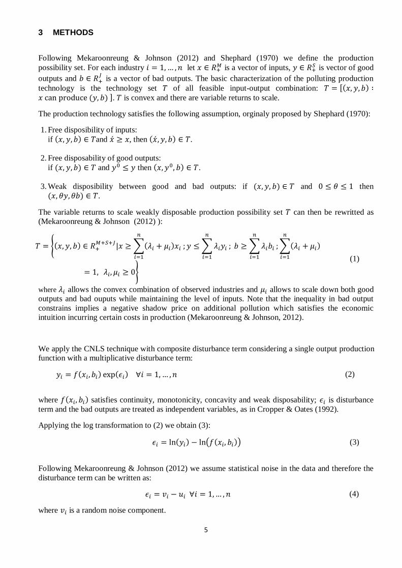
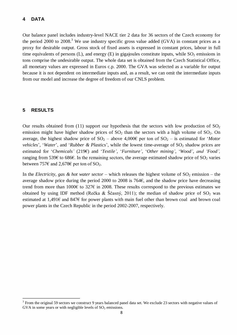
Our results obtained from (11) support our hypothesis that the sectors with low production of SO2

emission might have higher shadow prices of SO2 than the sectors with a high volume of SO2. On

average, the highest shadow price of SO2 – above 4,000€ per ton of SO2 – is estimated for ‘Motor

vehicles’, ‘Water’, and ‘Rubber & Plastics’, while the lowest time-average of SO2 shadow prices are

estimated for ‘Chemicals’ (219€) and ‘Textile’, ‘Furniture’, ‘Other mining’, ‘Wood’, and ‘Food’,

ranging from 539€ to 686€. In the remaining sectors, the average estimated shadow price of SO2 varies

between 757€ and 2,678€ per ton of SO2.

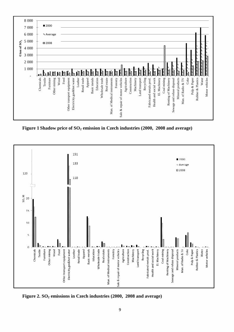
In the Electricity, gas & hot water sector – which releases the highest volume of SO2 emission – the

average shadow price during the period 2000 to 2008 is 764€, and the shadow price have decreasing

trend from more than 1000€ to 327€ in 2008. These results correspond to the previous estimates we

obtained by using IDF method (Rečka & Ščasný, 2011); the median of shadow price of SO2 was

estimated at 1,491€ and 847€ for power plants with main fuel other than brown coal and brown coal

power plants in the Czech Republic in the period 2002-2007, respectively.

3 From the original 59 sectors we construct 9 years balanced panel data set. We exclude 23 sectors with negative values of

GVA in some years or with negligible levels of SO2 emissions.

9

Figure 1 Shadow price of SO2 emission in Czech industries (2000, 2008 and average)

Figure 2. SO2 emissions in Czech industries (2000, 2008 and average)

-

1 000

2 000

3 000

4 000

5 000

6 000

7 000

8 000

Ch

emic

als

Tex

tile

Furn

iture

Oth

er m

inin

g

Wo

od

Foo

d

Oth

er t

ran

sport

eq

uip

men

t

Ele

ctri

city

,gas

&ho

t w

ater

Lea

ther

Ret

ail

trad

e

Ap

par

el

Basi

c m

etal

s

Ed

uca

tion

Wh

ole

sale

tra

de

Rea

l es

tate

Man

. of

Med

ical

inst

rum

ents

Fore

stry

Sal

e &

rep

air

of

mo

tor

veh

icle

s

Ag

ricu

ltu

re

Co

nst

ruct

ion

Mac

hin

ery

Lan

d t

ran

spo

rt

Rec

ycl

ing

Fab

rica

ted

met

als

pro

d.

Hea

lth

an

d s

oci

al w

ork

El.

Mac

hin

ery

Co

al m

inin

g

Ren

tin

g o

f M

ach

iner

y

Sew

age

and

ref

use

dis

posa

l

Min

eral

pro

du

cts

Man

. of

Rad

io &

TV

Co

ke

Pulp

& P

aper

Ru

bber

& P

last

ics

Wat

er

Moto

r veh

icle

s

€/t

on

of

SO

2

2000

Average

2008

10

Although the shadow price of SO2 significantly varies across the sectors, the shadow price decreases

over time in all of them, except manufacture of Other transport equipment and Retail trade (Figure 1).

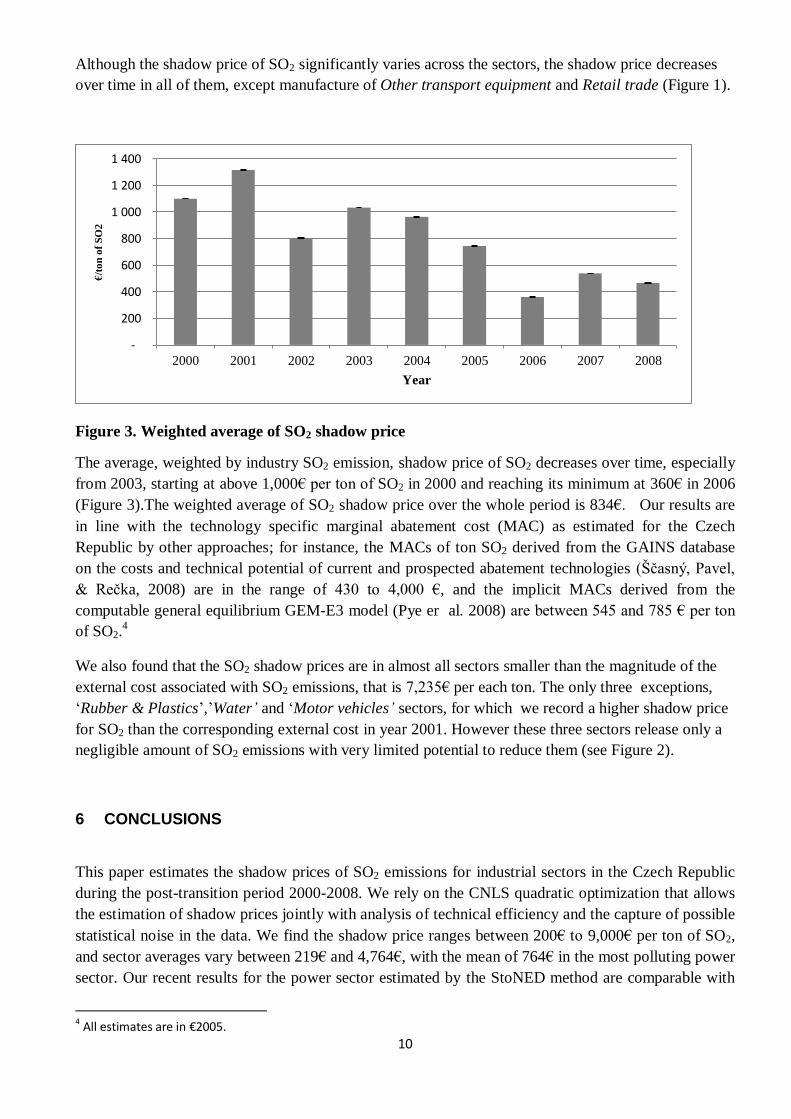
Figure 3. Weighted average of SO2 shadow price

The average, weighted by industry SO2 emission, shadow price of SO2 decreases over time, especially

from 2003, starting at above 1,000€ per ton of SO2 in 2000 and reaching its minimum at 360€ in 2006

(Figure 3).The weighted average of SO2 shadow price over the whole period is 834€. Our results are

in line with the technology specific marginal abatement cost (MAC) as estimated for the Czech

Republic by other approaches; for instance, the MACs of ton SO2 derived from the GAINS database

on the costs and technical potential of current and prospected abatement technologies (Ščasný, Pavel,

& Rečka, 2008) are in the range of 430 to 4,000 €, and the implicit MACs derived from the

computable general equilibrium GEM-E3 model (Pye er al. 2008) are between 545 and 785 € per ton

of SO2.4

We also found that the SO2 shadow prices are in almost all sectors smaller than the magnitude of the

external cost associated with SO2 emissions, that is 7,235€ per each ton. The only three exceptions,

‘Rubber & Plastics’,’Water’ and ‘Motor vehicles’ sectors, for which we record a higher shadow price

for SO2 than the corresponding external cost in year 2001. However these three sectors release only a

negligible amount of SO2 emissions with very limited potential to reduce them (see Figure 2).

6 CONCLUSIONS

This paper estimates the shadow prices of SO2 emissions for industrial sectors in the Czech Republic

during the post-transition period 2000-2008. We rely on the CNLS quadratic optimization that allows

the estimation of shadow prices jointly with analysis of technical efficiency and the capture of possible

statistical noise in the data. We find the shadow price ranges between 200€ to 9,000€ per ton of SO2,

and sector averages vary between 219€ and 4,764€, with the mean of 764€ in the most polluting power

sector. Our recent results for the power sector estimated by the StoNED method are comparable with

4 All estimates are in €2005.

-

200

400

600

800

1 000

1 200

1 400

2000 2001 2002 2003 2004 2005 2006 2007 2008

€/t

on

of

SO

2

Year

11

our previous estimates of the SO2 shadow prices that we estimated on the firm-level data from power

sector by following the non-parametric method based on the output distance function.

Our findings show a strong decreasing trend in the average magnitude of the shadow prices over time,

especially during 2001-2006. We note that the Czech Republic became a full member of the European

Union on May 1st, 2004, and from this time Czech firms can freely participate in the European

economic market and hence import advanced technologies without paying duties.

We also conclude that current regulation is far from the economic optimum, since in many sectors the

estimated SO2 shadow prices are much lower than the marginal damage cost, that is 7,235€ per ton of

SO2. For example, the average SO2 shadow prices in the two most emitting sectors – ‘Electricity, gas

& hot water’ and ‘Chemical’s – are 769€, or 219€, respectively.

The magnitude of shadow prices of SO2 emissions is also very far from the rates of SO2 emission

charges being currently enforced, having its rate below 40€ per ton (Máca et al., 2012). Considering

the magnitude of the shadow prices, we also conclude that to date air quality regulation based on

market-based instruments in the Czech Republic have been ineffective and economically sub-optimal.

As shown by Máca et al. (2012), the level of internalization of the external costs associate with air

quality pollutants and attributable to the power sector has remained rather low, up to 55% in the case

of coal-fired power plants. As of 2016, a new pricing system for SO2 discharges will be introduced in

the Czech Republic, which proposes a gradual increase in the charge from actual 36 €/ton of SO2 to

175 €/ ton after 2021. Despite this new regulation, the new level of emission charge rate is at least one

order of magnitude lower than our estimate of shadow prices for SO2 emissions.

Assuming full efficiency in this study – contrary to Lee (2002) – our estimates of shadow prices may

be biased slightly upward. We are aware of the fact that the top-down approach, as followed in this

analysis, can’t fully reveal all aspects of the costs that in reality, all play their role. In particular,

additional costs associated with abatement in industrial companies can be involved by other non-

environmental regulations, such as requirements on higher safety standards. This analysis merely aims

at estimation of the shadow prices of undesirable outputs, such as air emissions, and it cannot serve to

examine the effect of all other possible factors on the abatement costs, cost effectiveness or on the

emission reduction potential.

ACKNOWLEDGEMENTS

The research has been supported by Czech Science Foundations’ project PEPCI no. 13-24814S. This

support is gratefully acknowledged. Special thanks belong to Andrew L. Johnson for his help with the

GAMS code. Responsibility for any errors remains with the authors.

REFERENCES

Aigner, D., Lovell, C. A. K., & Schmidt, P. (1977). Formulation and Estimation of Stochastic Frontier Production Function Models. Journal of Econometrics, 6, 21–37.

Atkinson, S. E., & Dorfman, J. H. (2005). Bayesian measurement of productivity and efficiency in the presence of undesirable outputs: crediting electric utilities for reducing air pollution. Journal of Econometrics, 126(2), 445–468. doi:10.1016/j.jeconom.2004.05.009

12

Bauman, Y., Lee, M., & Seeley, K. (2008). Does Technological Innovation Really Reduce Marginal Abatement Costs? Some Theory, Algebraic Evidence, and Policy Implications. Environmental and Resource Economics, 40(4), 507–527. doi:10.1007/s10640-007-9167-7

Boyd, G., Molburg, J., & Prince, R. (1996). Alternative Methods of Marginal Abatement Cost Estimation: Non-parametric Distance Functions. Proceedings of the USAEE/IAEE 17th Conference.

Coggins, J. S., & Swinton, J. R. (1996). The Price of Pollution: A Dual Approach to Valuing SO2Allowances. Journal of Environmental Economics and Management, 30(1), 58–72. doi:10.1006/jeem.1996.0005

Cropper, M. L., & Oates, W. E. (1992). Environmental Economics: A Survey. Journal of Economic Literature, 30(2), 675–740. Retrieved from http://ideas.repec.org/a/aea/jeclit/v30y1992i2p675-740.html

EEA. (2014). Air pollution fact sheet 2014 - Czech Republic. Retrieved from http://www.eea.europa.eu/themes/air/air-pollution-country-fact-sheets-2014/czech-republic-air-pollutant-emissions/view

Eurostat. (20115). Gross value added and income by A*10 industry breakdowns. Retrieved January 22, 2015, from http://ec.europa.eu/eurostat/data/database?ticket=ST-2348633

Färe, R., Grosskopf, S., Lovell, C. A. K., & Yaisawarng, S. (1993). Derivation of Shadow Prices for Undesirable Outputs: a Distance Function Approach. The Review of Economics and Statistics, 75(2), 374–380.

Färe, R., Grosskopf, S., & Nelson, J. (1990). On Price Efficiency. International Economic Review, 31(3), 709–720. Retrieved from http://www.jstor.org/stable/2527170#references_tab_contents

Färe, R., Grosskopf, S., Noh, D.-W., & Weber, W. (2005). Characteristics of a polluting technology: theory and practice. Journal of Econometrics, 126(2), 469–492. doi:10.1016/j.jeconom.2004.05.010

Gupta, M. (2006). Costs of Reducing Greenhouse Gas Emissions: A Case Study of India’s Power Generation Sector. SSRN Electronic Journal. doi:10.2139/ssrn.951455

Hailu, A., & Veeman, T. S. (2000). Environmentally Sensitive Productivity Analysis of the Canadian Pulp and Paper Industry , 1959-1994:An Input Distance Function Approach. Journal of Environmental Economics and Management, 40, 251–274.

Henderson, D. J., Kumbhakar, S. C., Parmeter, C. F., & Sun, K. (n.d.). Constrained Nonparametric Estimation of the Morishima Elasticity of Complementarity : Application to Norwegian Timber Production, 1–25.

Jondrow, J., Lovell, C. A. K., Materov, I. S., & Schmidt, P. (1982). On the Estimation of Technical Inefficiency in the Stochastic Frontier Production Function Model. Journal of Econometrics, 19, 233–238.

Kuosmanen, T., & Johnson, A. (2008). Data Envelopment Analysis as Nonparametric Least Squares Regression. SSRN Electronic Journal, 1–30. doi:10.2139/ssrn.1158252

Kuosmanen, T., & Kortelainen, M. (2012). Stochastic non-smooth envelopment of data: semi-parametric frontier estimation subject to shape constraints. Journal of Productivity Analysis, 38(1), 11–28. doi:10.1007/s11123-010-0201-3

Kwon, O. S., & Yun, W.-C. (1999). Estimation of the marginal abatement costs of airborne pollutants in Korea’s power generation sector. Energy Economics, 21(6), 547–560. doi:10.1016/S0140-9883(99)00021-3

13

Lee, J.-D., Park, J.-B., & Kim, T.-Y. (2002). Estimation of the shadow prices of pollutants with production/environment inefficiency taken into account: a nonparametric directional distance function approach. Journal of Environmental Management, 64(4), 365–375. doi:10.1006/jema.2001.0480

Lee, M. (2005). The shadow price of substitutable sulfur in the US electric power plant: a distance function approach. Journal of Environmental Management, 77(2), 104–10. doi:10.1016/j.jenvman.2005.02.013

Máca, V., Melichar, J., & Ščasný, M. (2012). Internalization of External Costs of Energy Generation in Central and Eastern European Countries. Special Issue on the Experience with Environmental Taxation, Journal of Environment & Development, 21(2), 181–197. Retrieved from http://jed.sagepub.com/content/21/2/181.abstract

Maradan, D., & Vassiliev, A. (2005). Marginal costs of carbon dioxide abatement: Empirical evidence from cross-country analysis. REVUE SUISSE D ECONOMIE ET DE …, 1–32. Retrieved from http://www.cer.ethz.ch/wif/wif/resec/sgvs/011.pdf

Marklund, P.-O. (2003). Analyzing interplant marginal abatement cost differences: A directional output distance function approach (No. 618). Umeå Economic Studies. Retrieved from http://ideas.repec.org/p/hhs/umnees/0618.html

Mekaroonreung, M., & Johnson, A. L. (2012). Estimating the shadow prices of SO2 and NOx for U.S. coal power plants: A convex nonparametric least squares approach. Energy Economics, 34(3), 723–732. doi:10.1016/j.eneco.2012.01.002

Murty, M. N., Kumar, S., & Dhavala, K. K. (2006). Measuring environmental efficiency of industry: a case study of thermal power generation in India. Environmental and Resource Economics, 38(1), 31–50. doi:10.1007/s10640-006-9055-6

Olabi, A. G. (2014). 100% sustainable energy. Energy, 77, 1–5. doi:10.1016/j.energy.2014.10.083

Park, H., & Lim, J. (2009). Valuation of marginal CO2 abatement options for electric power plants in Korea. Energy Policy, 37(5), 1834–1841. doi:10.1016/j.enpol.2009.01.007

Peng, Y., Wenbo, L., & Shi, C. (2012). The Margin Abatement Costs of CO2 in Chinese industrial sectors. Energy Procedia, 14(2011), 1792–1797. doi:10.1016/j.egypro.2011.12.1169

Preiss, P., Friedrich, R., & Klotz, V. (2008). Report on the procedure and data to generate averaged/aggregated data. Deliverable n° 1.1 - RS 3a R&D Project NEEDS–New Energy Externalities Developments for Sustainability (Vol. Project re). Retrieved from http://opus.bath.ac.uk/9773/

Pye, S., Holland, M., Regemorter, D. Van, Wagner, A., & Watkiss, P. (2008). Analysis of the Costs and Benefits of Proposed Revisions to the National Emission Ceilings Directive. NEC CBA Report 3. National Emission Ceilings for 2020 based on the 2008 Climate & Energy Package. AEA Energy & Environment; Prepared for the European Com. NEC CBA Report 3. National Emission Ceilings for 2020 based on the 2008 Climate & Energy Package.

Rečka, L., & Ščasný, M. (2011). Emission Shadow Price Estimation Based on Distance Function: a Case of the Czech Energy Industry. In INTERNATIONAL DAYS OF STATISTICS AND ECONOMICS (pp. 543–554).

Rezek, J. P., & Campbell, R. C. (2007). Cost estimates for multiple pollutants: A maximum entropy approach. Energy Economics, 29(3), 503–519. doi:10.1016/j.eneco.2006.01.005

14

Salnykov, M., & Zelenyuk, V. (2004). Estimation of Environmnetal Inefficiencies and Shadow prices of pollutants: A Cross-Country Approach. Retrieved from http://www.kse.org.ua/uploads/file/library/2004/Salnykov.pdf

Ščasný, M., & Máca, V. (2009). Market-Based Instruments in CEE Countries: Much Ado about Nothing. Rivista Di Politica Economica, 99(3), 59–91. Retrieved from http://econpapers.repec.org/RePEc:rpo:ripoec:v:99:y:2009:i:3:p:59-91

Ščasný, M., Pavel, J., & Reč�ka, L. (2008). Analýza nákladů na snížení emisí znečišťujících látek vypouštěných do ovzduší stacionárními zdroji [Analysis of abatement cost of pollutants released by stationary sources]. R&D project SPII/4i1/52/07 MODEDR – “Modeling of Environmental Tax Reform Impacts: The Czech ETR Stage II” funded by the Ministry of the Environment of the Czech Republic. M1-annual report 2008.

Ščasný, M., Píša, V., Pollit, H., & Chewpreecha, U. (2009). Analyzing Macroeconomic Effects of Environmental Taxation in the Czech Republic with the Econometric E3ME Model. Czech Journal of Economics and Finance (Finance a Uver), 59(5), 460–491. Retrieved from http://ideas.repec.org/a/fau/fauart/v59y2009i5p460-491.html

Shephard, R. W. (1970). Theory of Cost and Production Functions. Princeton: Princeton University Press. Retrieved from http://www.jstor.org/stable/2230285

Swinton, J. R. (1998). At What Cost do We Reduce Pollution? Shadow Prices of SO2 Emissions. The Energy Journal, 19(4). doi:10.5547/ISSN0195-6574-EJ-Vol19-No4-3

Swinton, J. R. (2002). The Potential for Cost Savings in the Sulfur Dioxide Allowance Market: Empirical Evidence from Florida. Land Economics, 78(3), 390–404. doi:10.3368/le.78.3.390

Weinzettel, J., Havránek, M., & Ščasný, M. (2012). A consumption based indicator of external costs of electricity. Ecological Indicators, 17(June 2012), 68–76.

Wu, P.-I., Chen, C. T., & Liou, J.-L. (2013). The meta-technology cost ratio: An indicator for judging the cost performance of CO2 reduction. Economic Modelling, 35, 1–9. doi:10.1016/j.econmod.2013.06.028