Embed Size (px)
Citation preview
Shah, Roopam (2013) Efficiency of Banks using the Stochastic Frontier Approach: Evidence from India. [Dissertation (University of Nottingham only)] (Unpublished)
Access from the University of Nottingham repository: http://eprints.nottingham.ac.uk/26533/1/DISSERTATION_-_ROOPAM_SHAH.pdf
Copyright and reuse:
The Nottingham ePrints service makes this work by students of the University of Nottingham available to university members under the following conditions.
This article is made available under the University of Nottingham End User licence and may be reused according to the conditions of the licence. For more details see: http://eprints.nottingham.ac.uk/end_user_agreement.pdf
For more information, please contact [email protected]
1
EFFICIENCY OF BANKS USING THE STOCHASTIC
FRONTIER APPROACH: EVIDENCE FROM INDIA
ROOPAM PRADIP SHAH
MSc FINANCE AND INVESTMENT
2
ABSTRACT
This dissertation contributes to the banking efficiency literature by measuring the
efficiency of Indian banks for the period 2001-2011. It employs a Stochastic Distance
Function Approach and estimates the efficiency scores using three models - The Error
Correction Model, with and without Eta, and the Technical Efficiency Effects Model. The
results show that the Error Correction Model without Eta and the Technical Efficiency
Effects Model, both produced a substantially high mean efficiency score. The Error
Correction Model with Eta showed declining efficiency scores over the 11 year period.
However, the average efficiency score was higher than that of the Error Correction Model
without Eta which did not take into account time varying effects. Additionally, this study
also makes an attempt to determine the factors that influence the profitability of Indian
banks using the Profitability Model. However, none of the chosen variables had a
significant correlation with the profitability.
3
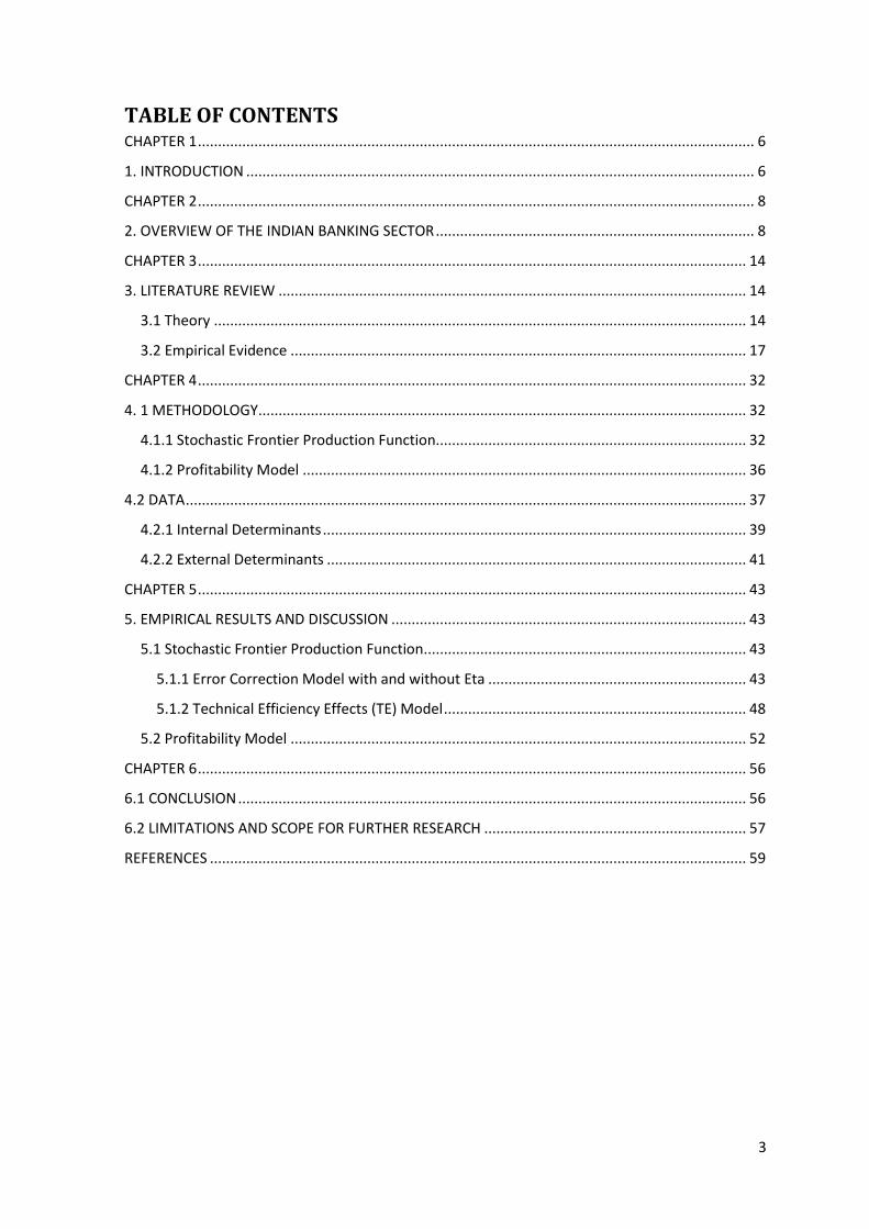
TABLE OF CONTENTS CHAPTER 1 .......................................................................................................................................... 6
1. INTRODUCTION .............................................................................................................................. 6
CHAPTER 2 .......................................................................................................................................... 8
2. OVERVIEW OF THE INDIAN BANKING SECTOR ............................................................................... 8
CHAPTER 3 ........................................................................................................................................ 14
3. LITERATURE REVIEW .................................................................................................................... 14
3.1 Theory .................................................................................................................................... 14
3.2 Empirical Evidence ................................................................................................................. 17
CHAPTER 4 ........................................................................................................................................ 32
4. 1 METHODOLOGY ......................................................................................................................... 32
4.1.1 Stochastic Frontier Production Function............................................................................. 32
4.1.2 Profitability Model .............................................................................................................. 36
4.2 DATA ........................................................................................................................................... 37
4.2.1 Internal Determinants ......................................................................................................... 39
4.2.2 External Determinants ........................................................................................................ 41
CHAPTER 5 ........................................................................................................................................ 43
5. EMPIRICAL RESULTS AND DISCUSSION ........................................................................................ 43
5.1 Stochastic Frontier Production Function................................................................................ 43
5.1.1 Error Correction Model with and without Eta ................................................................ 43
5.1.2 Technical Efficiency Effects (TE) Model ........................................................................... 48
5.2 Profitability Model ................................................................................................................. 52
CHAPTER 6 ........................................................................................................................................ 56
6.1 CONCLUSION .............................................................................................................................. 56
6.2 LIMITATIONS AND SCOPE FOR FURTHER RESEARCH ................................................................. 57
REFERENCES ..................................................................................................................................... 59
4
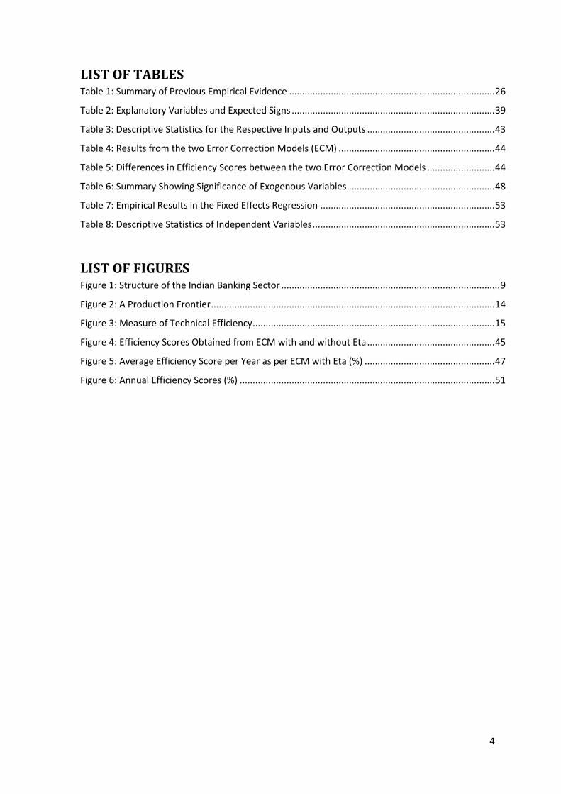
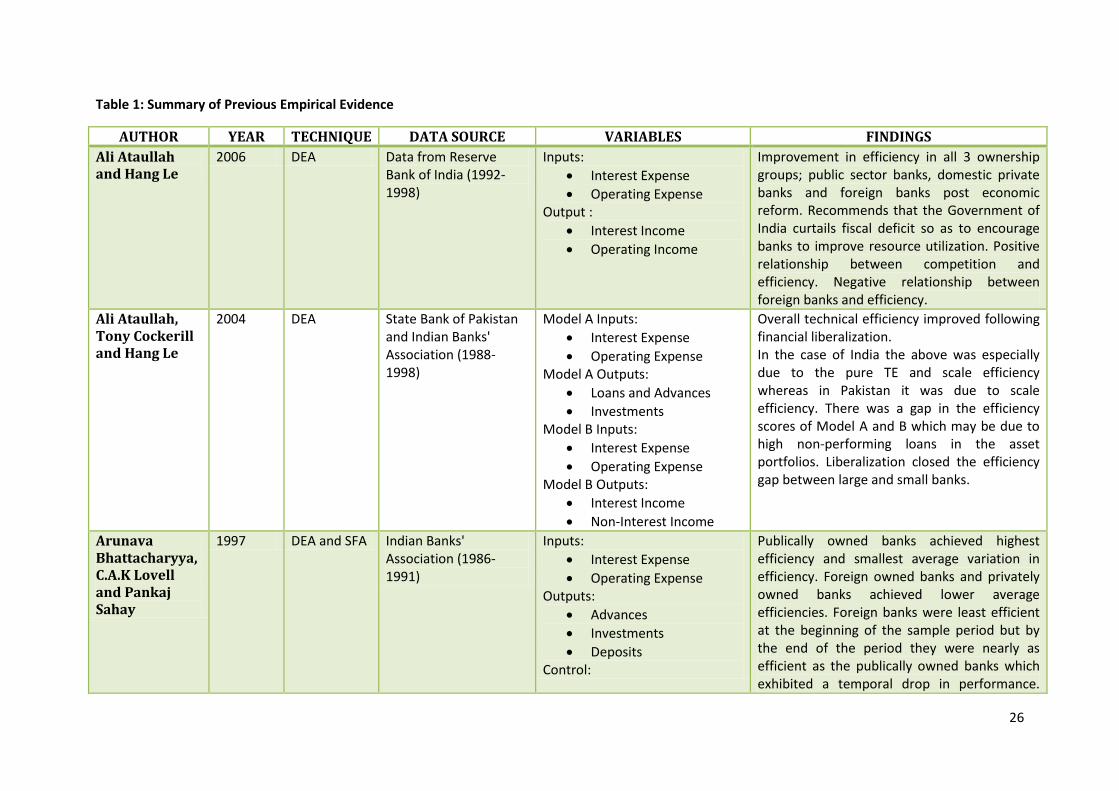
LIST OF TABLES Table 1: Summary of Previous Empirical Evidence ............................................................................... 26
Table 2: Explanatory Variables and Expected Signs .............................................................................. 39
Table 3: Descriptive Statistics for the Respective Inputs and Outputs ................................................. 43
Table 4: Results from the two Error Correction Models (ECM) ............................................................ 44
Table 5: Differences in Efficiency Scores between the two Error Correction Models .......................... 44
Table 6: Summary Showing Significance of Exogenous Variables ........................................................ 48
Table 7: Empirical Results in the Fixed Effects Regression ................................................................... 53
Table 8: Descriptive Statistics of Independent Variables ...................................................................... 53
LIST OF FIGURES Figure 1: Structure of the Indian Banking Sector .................................................................................... 9
Figure 2: A Production Frontier ............................................................................................................. 14
Figure 3: Measure of Technical Efficiency ............................................................................................. 15
Figure 4: Efficiency Scores Obtained from ECM with and without Eta ................................................. 45
Figure 5: Average Efficiency Score per Year as per ECM with Eta (%) .................................................. 47
Figure 6: Annual Efficiency Scores (%) .................................................................................................. 51

5
ACKNOWLEDGEMENTS
This dissertation would not have been possible without the guidance and help that was
provided by my supervisor, Dr. Maximilian Hall. I would like to take this opportunity to
thank him for the help and time he invested in this study. His constant feedback was of
great help when structuring the writing of this dissertation.
6
CHAPTER 1
1. INTRODUCTION
The former governor of the Reserve Bank of India (RBI); Dr. Bimal Jalan, stated in the Bank
Economists’ Conference (2002) that, “inefficiency in the use of resources, tolerance of
waste and slothfulness contributes to low productivity. The Indian banking sector suffers
from high costs and low productivity as reflected in high spreads. Therefore, the
challenge of managing transformation for the banking sector means moving from high
cost, low productivity and high spread to being more efficient, productive and
competitive.”
In recent years, substantial effort has been put into empirical studies focusing on
measuring the efficiency and productivity of the banking sector due to the importance of
this industry towards growth and stability of the economy. While a lot of the previous
literature has been focused on evaluating the performance of the banking sectors in
developed nations such as the United States of America (USA) and the United Kingdom
(UK), very few studies have analysed the performance of banking sectors in the
developing nations. Therefore, this paper focuses on measuring the efficiency of banks in
India. In most of the existing studies that have been carried out to estimate the efficiency
of Indian banks, the non-parametric approach of the Data Envelopment Analysis (DEA),
discussed in a later chapter, has been used. Hence, in this paper, the slightly less explored
measure of estimating efficiency, that is, the parametric approach of the Stochastic
Frontier Approach (SFA), discussed in a later chapter, has been employed to estimate the
Indian bank efficiency. Another reason for using the SFA is due to the fact that India is an
emerging economy where problems of measurement error and uncertain economic
environments are more likely to prevail.
Furthermore, earlier studies have emphasised the importance of estimating cost and
profit efficiency measures. However, since the banking industry uses multiple-output and
multiple-input production technology, a stochastic distance function approach is
considered more appropriate in this paper, without requiring input prices and making
behavioural assumptions. Another reason for using the distance function approach is that
7
since India is a developing country with quite a substantial gap between the rich and the
poor and also the fact that there are regional rural banks, it is difficult to be conclusive as
to whether such banks aim to maximise their profits or minimise their costs.
Finally, another contribution of this paper is to verify which factors are significant
determinants of the profitability of Indian banks, which is carried out in the profitability
model where the dependent variable employed is Return on Average Equity (ROAE) which
is considered to be a measure of profitability. The variables used in this model are also
used in the Technical Efficiency Effects (TE) model to test whether the variables have an
influence on the efficiency scores of Indian banks.
The rest of this paper is organised as follows. Chapter 2 introduces the Indian banking
industry. Chapter 3 reviews previous literature on bank efficiency. Chapter 4 describes
the research methodologies, specifies empirical models and data. Chapter 5 presents the
results and discussion on the findings. Finally, Chapter 6 draws conclusions and provides
recommendations for further research and analysis.
8
CHAPTER 2
2. OVERVIEW OF THE INDIAN BANKING SECTOR
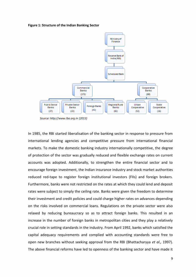
The Indian banking sector consists of a mixture of public, private and foreign ownerships.
Commercial banks dominate the industry, although the co-operative and regional rural
banks have a small business segment. The Indian banking sector consists of 2 categories;
scheduled and unscheduled banks. Scheduled banks are those which have been included
in the second schedule of the Reserve Bank of India (RBI) Act, 1934. So as to be included
under this Act, banks have to comply with certain conditions such as having a paid up
capital and reserves of a minimum of Rupees (Rs.) 0.5 million and assuring the RBI that
the banks’ affairs are conducted such that the interests of depositors are protected.
Scheduled banks can be further classified into Scheduled Commercial banks and
Scheduled Cooperative banks.
Unscheduled banks are those defined in clause (c) of Section 5 of the Banking Regulation
Act, 1949 (Jadhav, 2011). They function in the form of Local Area Banks (LAB) which was
established by the Government of India under a new scheme in 1996, whereby new
private banks with a local nature were to be set up with jurisdiction over a maximum of 3
neighbouring districts. The aim of this scheme was to provide easy mobility of funds of
rural and semi-urban districts (D&B, 2013). The above classifications and the number of
banks under each sub-section as at 31st March 2012 can be shown in Figure 1 below:
9
Figure 1: Structure of the Indian Banking Sector
In 1985, the RBI started liberalisation of the banking sector in response to pressure from
international lending agencies and competitive pressure from international financial
markets. To make the domestic banking industry internationally competitive, the degree
of protection of the sector was gradually reduced and flexible exchange rates on current
accounts was adopted. Additionally, to strengthen the entire financial sector and to
encourage foreign investment, the Indian insurance industry and stock market authorities
reduced red-tape to register foreign institutional investors (FIIs) and foreign brokers.
Furthermore, banks were not restricted on the rates at which they could lend and deposit
rates were subject to simply the ceiling rate. Banks were given the freedom to determine
their investment and credit policies and could charge higher rates on advances depending
on the risks involved on commercial loans. Regulations on the private sector were also
relaxed by reducing bureaucracy so as to attract foreign banks. This resulted in an
increase in the number of foreign banks in metropolitan cities and they play a relatively
crucial role in setting standards in the industry. From April 1992, banks which satisfied the
capital adequacy requirements and complied with accounting standards were free to
open new branches without seeking approval from the RBI (Bhattacharyya et al., 1997).
The above financial reforms have led to openness of the banking sector and have made it
10
healthy, sound, well-capitalised and primarily; internationally competitive (Dwivedi and
Charyulu, 2011).
The main regulator of banks in India is the central bank; the Reserve Bank of India (RBI)
(Wolters Kluwer Financial Services, 2013). The RBI was established on 1st April 1935 in
accordance with the Reserve Bank of India Act, 1934. It comprised of a share capital of Rs.
50 million which was divided into Rs. 100 per share fully paid and was wholly-owned by
private equity-holders initially. The Government held shares worth Rs. 220,000 in nominal
value. In 1949, the RBI was nationalised and had three major objectives which were
intended to be satisfied; to regulate the issues of bank notes, to maintain reserves with a
view of securing monetary stability and to operate the credit and currency system of the
country to its advantage (India Finance and Investment Guide, 2013).
The 8 main functions of the Reserve Bank of India are described below:
Bank of Issue – One of the primary functions of central banks is the formulation and
implementation of monetary policy. In the case of India, the basic roles of the RBI as
articulated in the Preamble to the RBI Act, 1934 are: “to regulate the issue of Bank notes
and the keeping of reserves with a view to securing monetary stability in India and
generally to operate the currency and credit system of the country to its advantage.”
Hence, the main objective of the monetary policy is to promote economic growth and
maintain price stability (Reserve Bank of India, 2010).
Issuer of Currency – To meet the required statutory goals from Section 22 of the RBI Act,
1934, one of the primary roles of the central bank is to manage the currency. Hence, the
RBI along with the Government of India is in charge of the design, production and
management of the Rupee. Their objective is to ensure that an adequate supply of clean
and genuine money exists in the economy. Together with the Indian Government, the RBI
tries to develop ways to reduce the risk of forgery of currency notes (Reserve Bank of
India, 2010).
Banker to Government – The RBI acts as the Governments’ banker, agent and adviser. It
has the responsibility to transact Government business by keeping cash balances as
interest-free deposits, making and/or receiving payments on behalf of the Government
11
and carrying out its exchange remittances and other banking operations. Additionally, the
RBI aids the Union and State in floating new loans and in managing public debt. According
to the India Finance and Investment Guide (2013), the RBI also advises the Government
on banking and monetary matters.
Banker to Banks and Lender of Last Resort – The RBI acts as the bankers’ bank. According
to the Banking Companies Act, 1949, each bank was required to maintain a current
account with the Reserve Bank with cash equivalent to 5% of its demand liabilities and 2%
of its liabilities in India. However, in 1962, banks were required to maintain cash reserves
worth 3% of their aggregate deposit liabilities (India Finance and Investment Guide,
2013). Despite being the bankers’ bank, the RBI also acts as the ‘lender of last resort’. This
means that when a solvent bank is having temporary liquidity problems, the RBI will come
to their rescue by making available to them the necessary liquidity that no one else is
ready to provide. The RBI would act as the ‘lender of last resort’ only during periods when
the resources of member banks have been exhausted. It would help individual member
banks who are undergoing a difficult time if the RBI is assured that the bank under
consideration is a strong bank (Reserve Bank of India, 2013). Additionally, scheduled
banks can borrow from the RBI on the basis of eligible securities or by getting financial
accommodation during periods of need or stringency by re-discounting bills of exchange
(India Finance and Investment Guide, 2013). It provides such assistance for the
betterment of depositors and to avoid the adverse effects of the bank undergoing
insolvency which may adversely affect the financial stability of the banking sector and
thus, the economy as a whole (Reserve Bank of India, 2010).
Financial Regulation and Supervision – The RBI’s role is to ensure the system’s safety and
soundness regularly such that protection of depositors’ interest is administered through a
regulatory framework and so that overall financial stability is sustained through various
policy measures such as on-site inspection and off-site monitoring(Reserve Bank of India,
2010). On-site inspection is carried out annually and focuses on internationally adopted
CAMELS model, i.e. capital adequacy, asset quality, management, earning, liquidity and
system and control. Once the inspection has been carried out, the top management of
the RBI sends supervisory letters to the top management of the banks indicating the
12
major areas of supervisory concern that need immediate attention. It also holds
supervisory discussions and draws up an action plan that may be monitored.
Off-site monitoring was introduced in 1995 for domestic operation of banks. Its primary
goal is to monitor the financial health of banks between two on-site inspections so as to
identify those banks which have shown some financial deterioration and may need
additional supervision. It therefore provides timely corrective action (Reserve Bank of
India, 2013).
Foreign Exchange Reserves Management – The RBI is the custodian of India’s foreign
exchange reserves and is responsible for managing their investment. RBI’s reserve
management function has developed due to two reasons. Firstly, the share of foreign
currency assets in the balance sheet of the bank has increased significantly. Secondly,
since exchange rates and interest rates fluctuate, it has become a challenge to preserve
the value of reserves and achieve reasonable returns on them. Therefore, the main
parameters of RBI’s policies for foreign exchange reserve management are safety,
liquidity and returns (Reserve Bank of India, 2010).
Controller of Credit – The RBI has the authority to influence the amount of credit created
by banks in India by either changing the Bank rate or through open market operations.
The RBI also has the power to review the accounts of commercial banks. Since it is the
supreme banking authority, it holds the cash reserves of all scheduled banks, controls
banks’ credit operations through quantitative and qualitative controls, uses inspection,
licensing and calling for information so as to take control of the banking system and,
lastly, it acts as the lender of last resort by providing re-discount facilities to scheduled
banks (India Finance and Investment Guide, 2013).
Promotional Functions – The RBI’s role is to promote sound banking habits, ensure that
banking facilities are available to rural and semi-urban areas and to establish and
encourage new specialised financing agencies (Reserve Bank of India, 2010).
The 2007-2008 financial turmoil did not affect the developed countries alone, but also
emerging economies such as India. India could not be insulated from the global financial
crisis despite having no direct exposure to the sub-prime mortgage assets or the failed
13
institutions which were the main origins of the financial meltdown. This was despite
India’s rapid integration with the world over the last decade as shown by, firstly; it’s two-
way trade statistics as a proportion of GDP, which grew from 21.2% in 1997-98 to 34.7%
in 2007-08 and secondly; the ratio of total external transactions to GDP which more than
doubled from 46.8% in 1997-98 to 117.4% in 2007-08 (Reserve Bank of India, 2010).
In 2008-09, India’s economic growth declined by 2.1% from the 8.8% average growth rate
in the previous five years to 6.7% (Bajpai, 2011). Following the collapse of Lehman
Brothers, Indian financial markets experienced a decline in net capital inflows from US$
17.3 billion in April-June 2007 to US$ 13.2 billion in April-June 2008 (Mohan, 2008).
Additionally, India’s stock market index (Sensex) experienced a significantly downward
movement due to an approximate US$ 11 billion sell off by FIIs (Lakshman, 2008), which
led to Sensex plunging from the 21,000 mark in January 2008 to below 10,000 in October
2008 (Kundu, 2008). Additionally, substantial pressure on dollar liquidity in the domestic
foreign exchange market was experienced and this resulted in: pressure on the Balance of
Payments outlook, the Indian rupee and increased volatility in the foreign exchange
market (Sinha, 2013).
The Global Financial crisis has not substantially had negative impacts on the Indian
banking sector since they have minimal exposure to the asset markets of the developed
world. There are very few Indian bank branches abroad; hence the banking sector has not
experienced major losses and write-downs like in the case of financial institutions in
Western economies (Venkitaramanan, 2008). The reason as to why India has been
protected from the financial turmoil is because of the role of nationalised banks. The RBI
adopted strict regulation and conservative policies such that the banks in the economy
are insulated to some extent from travails in the Western countries (Kundu, 2008).
14
CHAPTER 3
3. LITERATURE REVIEW
3.1 Theory Efficiency is the ability of a decision making unit to maximise its output given a set of
inputs (output orientation) or to produce a certain amount of output with the minimum
amount of inputs (input orientation) (Del Hoyo et al., 2004; Kumbhakar and Lovell, 2000).
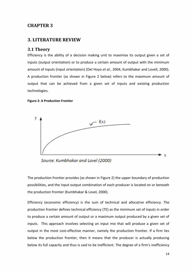
A production frontier (as shown in Figure 2 below) refers to the maximum amount of
output that can be achieved from a given set of inputs and existing production
technologies.
Figure 2: A Production Frontier
The production frontier provides (as shown in Figure 2) the upper boundary of production
possibilities, and the input-output combination of each producer is located on or beneath
the production frontier (Kumbhakar & Lovel, 2000).
Efficiency (economic efficiency) is the sum of technical and allocative efficiency. The
production frontier defines technical efficiency (TE) as the minimum set of inputs in order
to produce a certain amount of output or a maximum output produced by a given set of
inputs. This approach involves selecting an input mix that will produce a given set of
output in the most cost-effective manner, namely the production frontier. If a firm lies
below the production frontier, then it means that the producer is actually producing
below its full capacity and thus is said to be inefficient. The degree of a firm’s inefficiency
15
can be measured by how far below the production frontier the producer lies (Bera and
Sharma, 1999). Allocative efficiency measures the ability of a firm to fully utilise its inputs
given their prices (Kokkinou and Geo, 2009).
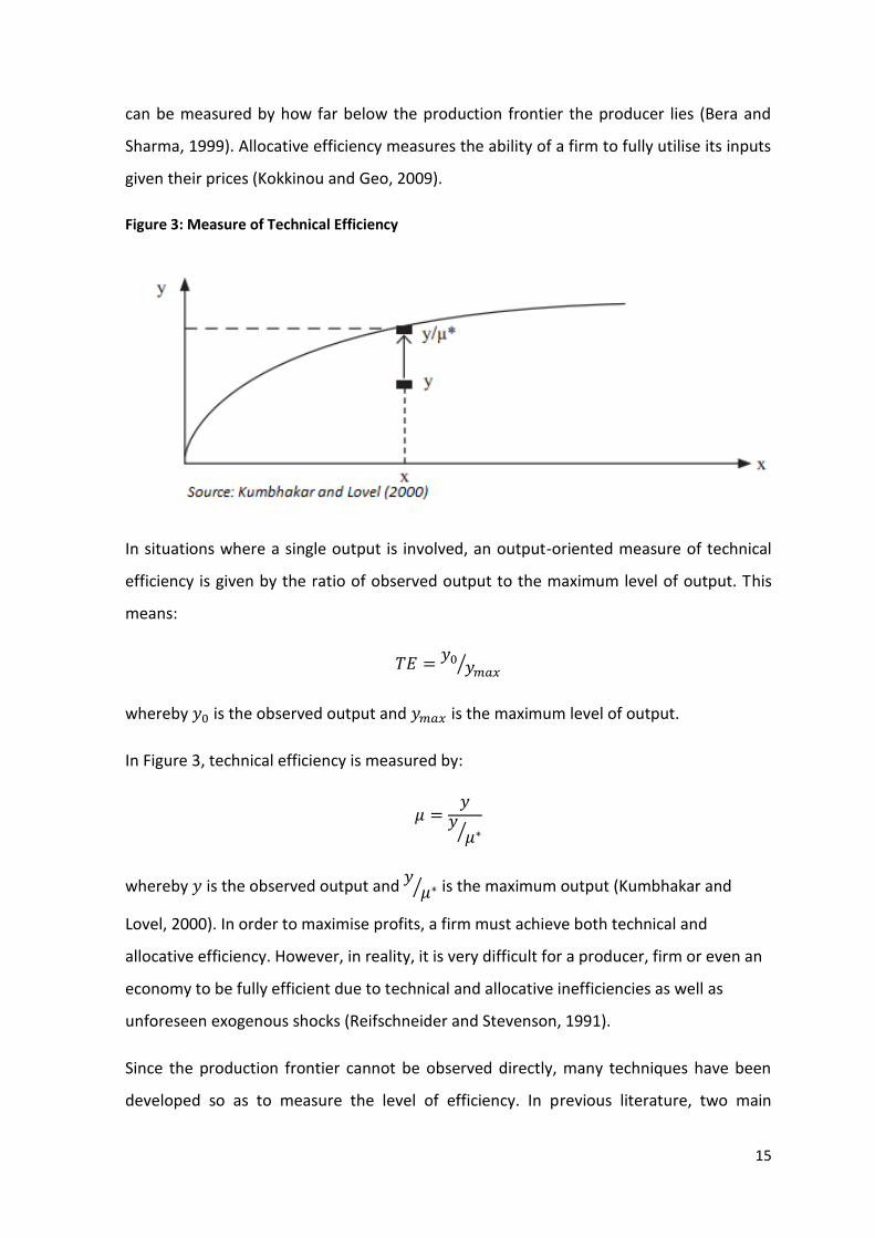
Figure 3: Measure of Technical Efficiency
In situations where a single output is involved, an output-oriented measure of technical
efficiency is given by the ratio of observed output to the maximum level of output. This
means:
whereby is the observed output and is the maximum level of output.
In Figure 3, technical efficiency is measured by:
whereby is the observed output and
is the maximum output (Kumbhakar and
Lovel, 2000). In order to maximise profits, a firm must achieve both technical and
allocative efficiency. However, in reality, it is very difficult for a producer, firm or even an
economy to be fully efficient due to technical and allocative inefficiencies as well as
unforeseen exogenous shocks (Reifschneider and Stevenson, 1991).
Since the production frontier cannot be observed directly, many techniques have been
developed so as to measure the level of efficiency. In previous literature, two main
16
approaches have been used to measure the efficiency of banks; non-parametric and
parametric approaches. Data Envelopement Analysis (DEA) lies in the former category
and estimates the efficient production frontier by using mathematical linear and
quadratic programming (Kiyota, 2009). Initial studies by Farrel (1957) and later by Aigner
and Chau (1968) used such techniques to estimate such frontiers (Sharma et al., 2012).
The main advantage of DEA is that it is a simple application and does not require one to
make assumptions about the functional form or shape of the production frontier.
However, its core disadvantage is that the technique is incapable of splitting up the
deviations of certain banks from the efficient production frontier into inefficiency and a
random error component. Instead, it regards the entire deviation as inefficiency
regardless of whether the deviation is due to inefficient operation or exogenous effects
that are outside the control of the firm (Kiyota, 2009).
To overcome the problems associated with DEA, parametric approaches such as the
Distribution-Free Approach (DFA) and the Stochastic Frontier Approach (SFA) have been
adopted and are regarded as more sophisticated techniques relative to non-parametric
approaches. The DFA does not make any assumptions on the statistical distribution of
inefficiency, but assumes that the efficiency of each individual firm is stable over time and
the accumulated random error component averages out to zero over time, thereby
leading to the residual term consisting of simply inefficiency (Deyoung, 1997). It uses a
panel dataset whereby a firm’s efficiency is estimated by taking the difference between
the average residual of the individual firm and that of the firm that lies on the efficient
production frontier. Some truncations are carried out to account for the possibility that
the random error may not fully average out to zero (Berger and Humphrey, 1997).
The stochastic frontier production model was initially developed by Aigner, Lovell and
Schmidt (1977) and Meeusen and Broeck (1977), and was later modified and applied by
Battese and Corra (1977) and Battese and Coelli (1995). The SFA is considered the most
appropriate tool for estimating firm level inefficiency because it includes both technical
and input allocative efficiencies. Unlike DEA, it decomposes the deviations into a random
error component and production unit inefficiency, thus taking into account noise effects
such as measurement error. It therefore assumes that the inefficiencies usually follow a
truncated, asymmetric, half-normal distribution since inefficiencies are non-negative,
17
whereas the random shocks are assumed to be normally distributed (Kamberoglou et al.,
2004). Another advantage of the SFA is that one can carry out hypothesis tests for the
existence of the inefficiency and the structure of production technology (Samad, 2009).
However, Greene (1990) suggests that other distributions may be more appropriate since
he believes that the half-normal distribution assumption of inefficiency is relatively
inflexible and it assumes that most firms are grouped near full efficiency which may be
inappropriate.
3.2 Empirical Evidence
In response to studies by Sarkar et al. (1998) and Bhaumik and Dimova (2004) who used
Ordinary Least Squares (OLS) to measure the efficiency of banks, Khatri (2004) used SFA
to measure the efficiency of Indian banks between 1995 and 2001 since his view was that
OLS estimation takes the goodness of fit through observations and assumes that all banks
are efficient which may be misleading because there may be a substantial difference in
the efficiency levels of banks. Since Return on Assets (ROA) is obtained when profits are
normalised by assets, Khatri (2004) uses ROA as an output measure since he believes it is
an appropriate measure of performance. He found that ownership has a significant
influence on bank performance and that private and foreign banks outperform publicly-
owned banks. Furthermore, the findings showed that income from fee-based services is a
factor that leads to inefficiency in banks.
Sharma et al. (2012) applied SFA on a pooled database to measure the technical efficiency
of 74 scheduled commercial banks in India over the period 2005-2006 to 2009-2010. The
study also aimed at identifying the factors influencing the level of bank efficiency. The
study was carried out using a Cobb-Douglas production functional and inefficiency model
and showed that commercial banks have shown an improvement in their efficiency levels
over the period and the relationship significantly depends on fixed assets and deposit
inputs. It was found that the priority sector advance to total advance ratio (PTA) and
public owned banks are found to have a positive and significant relationship with the
technical efficiency of banks. Moreover, the cash-to-deposit ratio had a positive, but not
significant influence on technical efficiency; and the deposit to total liability ratio was
found to have a significant negative effect on the banks’ technical efficiency. In contrast
to the findings of Khatri (2004), this study found that SBI and the Nationalised Bank group
18
are relatively more efficient than private and foreign banks in India and that the
inefficiency of banks was due to internal factors which were firm-specific.
Kumar and Arora (2010) carried out an Indian study during the post-reform period of
1991-1992 to 2006-2007 to examine whether the two techniques of efficiency
measurement, namely the SFA and the DEA, produce conflicting results. The authors
followed an intermediation approach since the primary function of banks is to
intermediate inputs into outputs. Therefore, the inputs they chose to include in their
model were wages (labour), fixed assets (capital) and deposits (demand deposits, savings
bank deposits and term deposits) to produce investments (government securities, both in
India and outside India, approved and non-approved securities) and advances (bills
purchased and discounted, cash credits, overdrafts etc. and term loans) which were their
output variables. Additionally, since banks do not produce a single homogenous product,
and instead are a multiple output case, a stochastic specification of banks was needed so
as to incorporate multiple inputs and outputs. This was carried out using a stochastic
output distance function. At the end of the study, it was found that findings of both the
DEA and the SFA differed in terms of relative efficiency scores, relative rankings of sample
banks and ability to identify high efficiency level and low efficiency level banks. The
authors recommended the DEA technique since it does not require any prior assumptions
about the nature of distribution of the inefficiency component, unlike the SFA.
Sensarma (2006) carried out a study to measure the efficiency of Indian banks using the
Stochastic Cost Frontier Approach and then, unlike other studies, the author estimated a
measure of productivity that included an efficiency term during the period 1986 to 2000.
The study followed a value-added approach whose output vector consisted of fixed
deposits, saving deposits, current deposits, investments, loans and advances and number
of branches. The number of branches was included since it was assumed to be a proxy for
the quality of services and size of bank transactions. The input vector consisted of labour
and capital and control variables and included a dummy for deregulation which took
value 1 for years 1993 and above, and zero otherwise; size is taken to be the log of total
assets and ownership dummies take value 1 if the bank belongs to the public sector,
private sector and new private sector. This study differed from other studies such as
those of Kumbhakar and Sarkar (2003) and Shanmugam and Das (2004) since both foreign
19
and new private (entrants) banks were included as separate groups in the analysis.
Furthermore, each category of deposit was taken as a separate element in the output
vector since they are considered to have differing characteristics and that banks’ strategy
concerning each group may be different. Findings of this study suggested that there has
been a decline in cost inefficiencies in the Indian banking sector and that deregulation has
played a role in this and in improving the productivity of banks since an increase in the
Total Factor Productivity was found. Additionally, like the findings of Bhaumik and Dimova
(2004) who estimated the efficiency of Indian banks in terms of profit measures, public
banks were found to be performing in line with private banks in terms of both cost
efficiency and productivity and that ownership was not a significant factor.
To calculate radial technical efficiency scores of 70 Indian commercial banks during 1986
to 1991, Bhattacharyya et al. (1997) used a two-step procedure of which the first
consisted of calculating technical efficiencies using the DEA and the second involved
explaining variation in calculated efficiencies using the SFA. Similar to the
recommendations of Kumar and Arora (2010), the authors of this study also suggested
that DEA is more suitable for evaluating the performance of Indian banks because of the
institutional framework in which they operate. Additionally, they stated that the use of
the SFA would be complicated since banks offer a wide range of financial services and
because of regulation and market imperfections which distort prices and make it difficult
to measure cost, revenue or profit efficiency. Hence, they thought that the best use of the
SFA was to analyse the variation in the technical efficiencies computed using the DEA. In
previous studies, the calculated efficiencies were regressed on a set of exogenous
variables using OLS or Tobit methods if the efficiencies were censored variables.
However, the authors found that this approach had a major problem that part of the
variation in the calculated efficiencies may remain unaccounted for, thereby being part of
the white noise error term and contaminating the estimated regression coefficients.
Therefore, to overcome this problem, the unexplained part of the efficiency variation was
separated from the white noise error component. The input vector included in the model
consisted of interest and operating expense, the output vector included advances,
investments and deposits and control variables included were the number of branches in
rural, sub-urban, urban and metropolitan areas, the ratio of priority sector lending to
20
total advances and the capital adequacy ratio. Findings of the study suggested that
publicly-owned banks achieved the highest average efficiency and the smallest average
variation in efficiency. Foreign and privately-owned banks achieved the lowest average
efficiency and the largest variation in performance, thereby showing that there may be
differences in managerial philosophy and greater adaptability of banks from various
foreign countries. However, foreign-owned banks exhibited above-average performance
in the last year of the study and were almost as efficient as public sector banks.
By looking at studies carried out on other developing countries, the banking sectors of
countries such as Turkey have recently undergone substantial growth due to financial
liberalisation that took place like in the case of India. Demir et al. (2005) carried out a
study to identify the key factors influencing the technical efficiency differentials among
Turkish commercial banks in the pre- and post-liberalisation periods by using a technical
inefficiency effects model. They found that loan quality, size, ownership of banks and
profitability positively and significantly affected the technical efficiencies of the banks in
the dataset. Their findings suggested that if effective regulatory measures are
implemented, this would improve the quality of the earning assets of commercial banks.
Additionally, if the government encourages mergers and acquisitions of private banks and
privatisation of state-owned banks, then this may lead to improvement in the overall
efficiency of banks in Turkey.
Kablan (2007) carried out a study on measuring the bank efficiency in West African
Economic Monetary Union (WAEMU) post banking sector reforms from 1993 to 1996. The
monetary policy produced results that were contrary to expectations of favouring sectors
that promoted economic growth. Instead, it resulted in a banking crisis in the late 80s and
early 90s, leading to failure of approximately 27 banks. To resolve the situation, the
banking system of WAEMU was restructured. Banks that failed were either liquidated or
privatised, in which case ownership was open to foreign and domestic investors.
Furthermore, WAMU Banking Commission was initiated to supervise banking activities
and the central bank replaced the administration method of monetary regulation with
market mechanisms to enhance flexibility. The author aimed to evaluate both, technical
and cost efficiency so as to identify the appropriate policies for increasing banks
efficiency. To carry out the above, he used both the DEA and the SFA. The former was
21
used to estimate the technical efficiency by using a combination of inputs to produce a
given output. The latter was used to estimate the cost efficiency. The DEA was used by
assuming both Constant Return to Scale (CRS) and Variable Return to Scale (VRS) since
the latter is more relevant to environments of imperfect competition in which banks
operate. On the other hand, the SFA was estimated using a trans-logarithmic function
model due to the multiplicity of bank functions. The variables used to estimate the cost
efficiency frontier were total costs (interests payable, operating expenses and
depreciation expenses out of total assets), deposits (amounts owed to credit institution
and to customers out of total assets), loans (loans and advances to credit institutions and
to customers out of total assets), PK (depreciation expenses and provisions for assets to
tangible and intangible assets), PL (personnel expenses/average number of workers per
year) and PF( interest payable and similar charges with credit institutions and
customers/borrowed capital). Findings suggested that mean efficiency scores were 67%
for cost efficiency, 76% and 85% for technical efficiency under CRS and VRS respectively.
It was found that local banks with private capital were more efficient followed by foreign
banks subsidiaries and state owned banks achieving the least technical and cost efficiency
scores. Additionally, it was found that although WAEMU banks implemented new
technology, this did not have influence in improving their technical efficiency. However,
findings suggested that scale economies did play an influential role in incorporating
technological changes.
Like India, China has also undergone several structural reforms in the financial sector
from the early 1980s to transform the banking sector from a state-owned, monopolistic
and policy-driven system to a multi-ownership, competitive and profit-oriented one, as
stated by Jiang et al. (2009). This study aimed to add to the study carried out by Paul et al.
(2000) who used a distance function in an SFA framework to estimate bank efficiency. It
employs a stochastic distance function approach and allows for multiple inputs and
outputs of production technology without requiring input prices or behavioural
assumptions. It uses a single-step procedure to overcome serious econometric problems
suffered by a two-step approach which is explained by Casu and Molyneux (2000) as a
process whereby efficiency scores are treated as data or indices followed by a linear
regression which explains the variation in efficiency scores. The study also adds to the
22
method of Berger et al. (2005) by jointly examining the static, selection and dynamic
effects of corporate governance changes on bank efficiency. Furthermore, the scholars
specify three models to measure the sensitivity of efficiency scores to the variation in
output and input definitions. Model 1 is an income-based model which has two inputs:
total interest expense and non-interest expense and two outputs: net interest income
and non-interest income. Model 2 is an earning-based model which includes total interest
expense and labour and physical capital as its two inputs and total loans, total deposits
and non-interest income as its three outputs. Model 3 is also an earning-based model
which includes three inputs: total interest expense, physical capital and labour and total
loans, total deposits and other earning assets as its three outputs. Additionally, as
suggested by the literature they also used a translog function. The study collected its
main data from 1995 to 2005 from Bankscope and the sample included the reform period
during which the banking system was moving towards market orientation. So as to
impose the homogeneity constraint and to reduce the problem of multicollinearity, net
interest income (Model 1) and total loans (Model 2 and 3) were used as normalisation
variables. The risk taking characteristics used were equity to total assets ratio as a proxy
of capital risk, loan loss reserve to total loans ratio as a measure of credit risk, interbank
borrowing to total deposits ratio as a proxy of market risk and total loans to total deposits
ratio as a representation of liquidity risk. Furthermore, GDP growth rate was used as a
proxy of the bank’s macroeconomic environment and a time trend was also included to
evaluate whether inefficiency is time-variant. An average efficiency of 70% was found,
whereby joint-stock and state-owned commercial banks were found to be the most
efficient bank group in all three models. Foreign banks were identified as the least
efficient bank group. They seemed to be more technically efficient in terms of income
generation rather than in earning assets. The authors suggested the use of both income-
based and earning assets-based models since they both analyse efficiency of banks’
operation from different aspects.
Cuesta and Orea (2002) carried out a study to test the temporal variation of technical
efficiency of Spanish savings banks from 1985 to 1998 and also tested whether merged
and non-merged banks have different levels and temporal patterns of technical efficiency.
As mentioned in the paper written by Jiang et al. (2009), this study also used a stochastic
23
output distance function to accommodate multiple output technology without
information about prices. The temporal variation of technical efficiency is modelled by
extending the Battese and Coelli approach so as to relax the monotonicity of the
temporal variation pattern of the efficiency term by adding a quadratic term and
permitting for different patterns of efficiency change (different error structures) between
merged and non-merged firms. This paper followed the Sealey and Lindley (1977)
approach of using labour, capital and deposits to produce earning assets. Therefore, the
variables that were thought to be relevant included: bonds, cash and other assets, loans
and non-interest income as the three outputs and the four inputs included were time and
savings deposits, other deposits and funds, labour (measured by personnel expenses) and
capital (measured by physical capital amortisation and other non-interest expenses). Non-
interest income was included as an output variable in an attempt to include off-balance
sheet activities such as securitisation, brokerage services and management of financial
assets for customers, all of which are deemed to be substantially important in the Spanish
banking sector. It was found that merged and non-merged firms both follow different
patterns of technical efficiency change. Merged firms followed a downward trend in
technical efficiency (the lowest being 83.9%) for the first 5 years showing that the
immediate effect of amalgamation was a decrease in technical efficiency. However, after
reorganisation of the merged firms, an improvement in technical efficiency was seen. The
conclusion that was reached was that mergers have some impact on technical efficiency
however, only a flexible model would be able to observe effects of mergers on technical
efficiency. They recommended future research to use more flexible specifications for the
efficiency variation, model the efficiency term using different distribution, to look at both
the theoretical and empirical effects of the distributions on the estimates and lastly, to
use a longer panel to apply the model.
Over the last 10 years, the banking sector of Central and Eastern Europe have slowly
developed from the traditional mono-bank system of the centrally-planned period to a
geographically and sector diversified two-tiered system. There has been a substantial
change in the competitive structure of the financial sector due to deregulation and
liberalisation, as well as significant privatisation and foreign participation. To examine the
cost and profit efficiency of banking sectors in 12 transition economies of Central and
24
Eastern Europe over the period 1993 to 2000, Yildirim and Philipattos (2003) used the
stochastic frontier approach (SFA) and the distribution free approach (DFA). They used a
two-stage estimation procedure, whereby, in the first stage, a translog was specified to
obtain efficiency estimates for the individual banks in the sample. In the second stage,
they analysed the potential correlates of efficiency by regressing the inefficiency scores
on various bank-specific and market-structure variables. In this study, X-efficiency was
referred to as the degree of managerial success on using inputs and outputs in such a way
so as to minimise costs and maximise profits. The dependent variable in the cost frontier
function was the logarithm of total cost which included the sum of interest expenses,
personnel expenses and other operating expenses. To impose linear input price
homogeneity, cost and input prices were normalised by price of capital before taking
logarithms. In the case of the profit frontier estimation, the same specification was used
however, profit and output variables were normalised by equity capital to control for
heteroscedasticity, scale biases and other estimation biases. An intermediation approach
was adopted whereby the three outputs included loans (sum of loan accounts
intermediated by banks less non-performing loans), investments (sum of total securities,
equity investments and other investments) and deposits (sum of demand, savings and
time deposits), whereas the three inputs included were borrowed funds, labour and
physical capital. Equity capital was adopted as the control variable since it controls for
managerial risk preferences in solving maximisation and minimisation problems.
Additionally, given the reality of high insolvency risks due to substantial non-performing
loans, including equity becomes important for the study of transition banking sector.
Moreover, equity constitutes an alternative to deposits in funding loans and investments.
Therefore, it was assumed to have a significant influence of costs and profits. Once the
efficiency scores were obtained, an explanatory analysis was carried out using bank-
specific and country-specific factors. Bank-specific factors included in the study were size
(log of total assets), capitalisation (book value of stockholders’ equity as a fraction of total
assets), risk (total loans over total assets and loan loss reserves as a fraction of gross
loans), funding (customer and short-term funding over total funds and interbank deposits
over total deposits) and off-balance sheet activity variables (off-balance sheet items as a
fraction of total assets). The country-specific factors included were the degree of
competition (using Panzar and Rosse (1987) H-statistic), market concentration (market
25
share of the three largest banks in the industry), GDP growth rate, a dummy variable to
distinguish between foreign and domestic banks, bank specialisation dummy variable to
differentiate between commercial and cooperative banks and lastly, a dummy variable to
separate publicly traded banks and private banks. The findings of the paper showed that
there was a relatively small difference between the average cost efficiency levels
produced by the SFA and DFA models of 72% and 77% respectively, thereby suggesting
that banks would have reduced their actual costs by 23 to 28% had they matched their
performance to the best-practice bank. In the case of profit efficiency levels, the SFA
estimates illustrated that approximately one-third of banks’ profits are lost to inefficiency,
whereas according to DFA, almost one-half of banks’ profits are forgone. The results of
the second stage regression suggested that large and well-capitalised banks are more
efficient. Furthermore, banks that heavily rely on deposits for funding their assets are
found to be more efficient and that there is a negative relation between problem loans
and efficiency. Additionally, it was found that the higher the intensity of competition, the
lower the cost efficiency, but the higher the profit efficiency and that, favourable
economic conditions only have a positive impact on the banks profit efficiency. Lastly,
foreign banks were found to be more cost efficient, but less profit efficient as compared
to domestically owned private and state-owned banks.
26
Table 1: Summary of Previous Empirical Evidence
AUTHOR YEAR TECHNIQUE DATA SOURCE VARIABLES FINDINGS
Ali Ataullah and Hang Le
2006 DEA Data from Reserve Bank of India (1992-1998)
Inputs:
Interest Expense
Operating Expense Output :
Interest Income
Operating Income
Improvement in efficiency in all 3 ownership groups; public sector banks, domestic private banks and foreign banks post economic reform. Recommends that the Government of India curtails fiscal deficit so as to encourage banks to improve resource utilization. Positive relationship between competition and efficiency. Negative relationship between foreign banks and efficiency.
Ali Ataullah, Tony Cockerill and Hang Le
2004 DEA State Bank of Pakistan and Indian Banks' Association (1988-1998)
Model A Inputs:
Interest Expense
Operating Expense Model A Outputs:
Loans and Advances
Investments Model B Inputs:
Interest Expense
Operating Expense Model B Outputs:
Interest Income
Non-Interest Income
Overall technical efficiency improved following financial liberalization. In the case of India the above was especially due to the pure TE and scale efficiency whereas in Pakistan it was due to scale efficiency. There was a gap in the efficiency scores of Model A and B which may be due to high non-performing loans in the asset portfolios. Liberalization closed the efficiency gap between large and small banks.
Arunava Bhattacharyya, C.A.K Lovell and Pankaj Sahay
1997 DEA and SFA Indian Banks' Association (1986-1991)
Inputs:
Interest Expense
Operating Expense Outputs:
Advances
Investments
Deposits Control:
Publically owned banks achieved highest efficiency and smallest average variation in efficiency. Foreign owned banks and privately owned banks achieved lower average efficiencies. Foreign banks were least efficient at the beginning of the sample period but by the end of the period they were nearly as efficient as the publically owned banks which exhibited a temporal drop in performance.
27
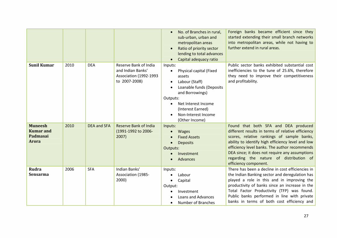
No. of Branches in rural, sub-urban, urban and metropolitan areas
Ratio of priority sector lending to total advances
Capital adequacy ratio
Foreign banks became efficient since they started extending their small branch networks into metropolitan areas, while not having to further extend in rural areas.
Sunil Kumar 2010 DEA Reserve Bank of India and Indian Banks' Association (1992-1993 to 2007-2008)
Inputs:
Physical capital (Fixed assets
Labour (Staff)
Loanable funds (Deposits and Borrowings)
Outputs:
Net Interest Income (Interest Earned)
Non-Interest Income (Other Income)
Public sector banks exhibited substantial cost inefficiencies to the tune of 25.6%, therefore they need to improve their competitiveness and profitability.
Muneesh Kumar and Padmasai Arora
2010 DEA and SFA Reserve Bank of India (1991-1992 to 2006-2007)
Inputs:
Wages
Fixed Assets
Deposits Outputs:
Investment
Advances
Found that both SFA and DEA produced different results in terms of relative efficiency scores, relative rankings of sample banks, ability to identify high efficiency level and low efficiency level banks. The author recommends DEA since; it does not require any assumptions regarding the nature of distribution of efficiency component.
Rudra Sensarma
2006 SFA Indian Banks' Association (1985-2000)
Inputs:
Labour
Capital Output:
Investment
Loans and Advances
Number of Branches
There has been a decline in cost efficiencies in the Indian Banking sector and deregulation has played a role in this and in improving the productivity of banks since an increase in the Total Factor Productivity (TFP) was found. Public banks performed in line with private banks in terms of both cost efficiency and
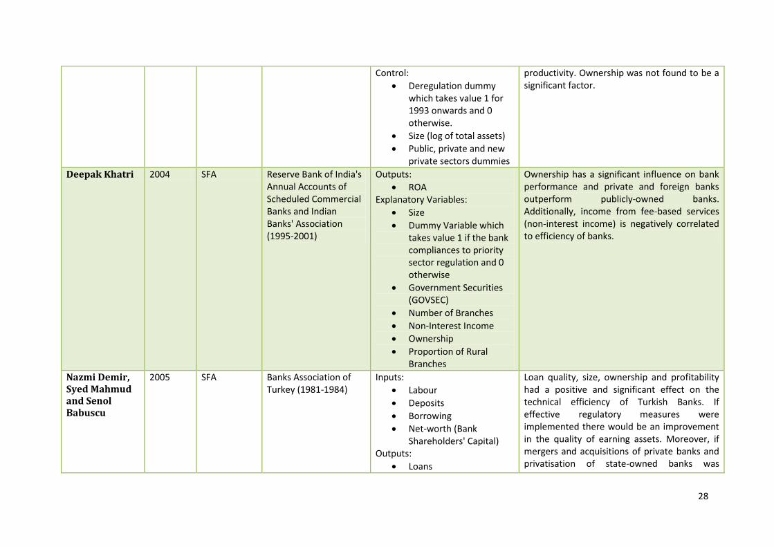
28
Control:
Deregulation dummy which takes value 1 for 1993 onwards and 0 otherwise.
Size (log of total assets)
Public, private and new private sectors dummies
productivity. Ownership was not found to be a significant factor.
Deepak Khatri 2004 SFA Reserve Bank of India's Annual Accounts of Scheduled Commercial Banks and Indian Banks' Association (1995-2001)
Outputs:
ROA Explanatory Variables:
Size
Dummy Variable which takes value 1 if the bank compliances to priority sector regulation and 0 otherwise
Government Securities (GOVSEC)
Number of Branches
Non-Interest Income
Ownership
Proportion of Rural Branches
Ownership has a significant influence on bank performance and private and foreign banks outperform publicly-owned banks. Additionally, income from fee-based services (non-interest income) is negatively correlated to efficiency of banks.
Nazmi Demir, Syed Mahmud and Senol Babuscu
2005 SFA Banks Association of Turkey (1981-1984)
Inputs:
Labour
Deposits
Borrowing
Net-worth (Bank Shareholders' Capital)
Outputs:
Loans
Loan quality, size, ownership and profitability had a positive and significant effect on the technical efficiency of Turkish Banks. If effective regulatory measures were implemented there would be an improvement in the quality of earning assets. Moreover, if mergers and acquisitions of private banks and privatisation of state-owned banks was
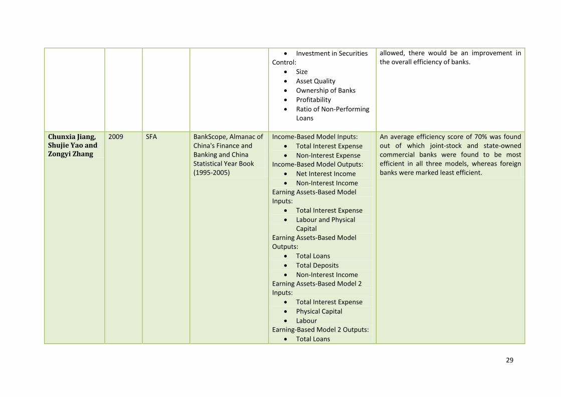
29
Investment in Securities Control:
Size
Asset Quality
Ownership of Banks
Profitability
Ratio of Non-Performing Loans
allowed, there would be an improvement in the overall efficiency of banks.
Chunxia Jiang, Shujie Yao and Zongyi Zhang
2009 SFA BankScope, Almanac of China's Finance and Banking and China Statistical Year Book (1995-2005)
Income-Based Model Inputs:
Total Interest Expense
Non-Interest Expense Income-Based Model Outputs:
Net Interest Income
Non-Interest Income Earning Assets-Based Model Inputs:
Total Interest Expense
Labour and Physical Capital
Earning Assets-Based Model Outputs:
Total Loans
Total Deposits
Non-Interest Income Earning Assets-Based Model 2 Inputs:
Total Interest Expense
Physical Capital
Labour Earning-Based Model 2 Outputs:
Total Loans
An average efficiency score of 70% was found out of which joint-stock and state-owned commercial banks were found to be most efficient in all three models, whereas foreign banks were marked least efficient.
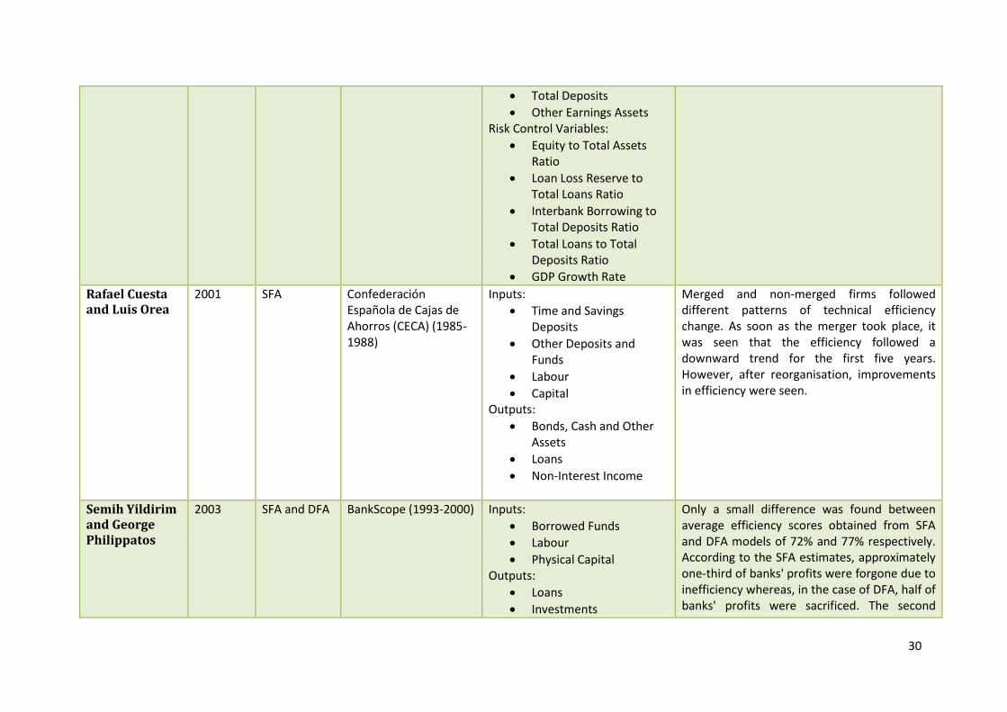
30
Total Deposits
Other Earnings Assets Risk Control Variables:
Equity to Total Assets Ratio
Loan Loss Reserve to Total Loans Ratio
Interbank Borrowing to Total Deposits Ratio
Total Loans to Total Deposits Ratio
GDP Growth Rate
Rafael Cuesta and Luis Orea
2001 SFA Confederación Española de Cajas de Ahorros (CECA) (1985-1988)
Inputs:
Time and Savings Deposits
Other Deposits and Funds
Labour
Capital Outputs:
Bonds, Cash and Other Assets
Loans
Non-Interest Income
Merged and non-merged firms followed different patterns of technical efficiency change. As soon as the merger took place, it was seen that the efficiency followed a downward trend for the first five years. However, after reorganisation, improvements in efficiency were seen.
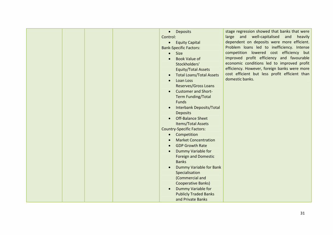
Semih Yildirim and George Philippatos
2003 SFA and DFA BankScope (1993-2000) Inputs:
Borrowed Funds
Labour
Physical Capital Outputs:
Loans
Investments
Only a small difference was found between average efficiency scores obtained from SFA and DFA models of 72% and 77% respectively. According to the SFA estimates, approximately one-third of banks' profits were forgone due to inefficiency whereas, in the case of DFA, half of banks' profits were sacrificed. The second
31
Deposits Control:
Equity Capital Bank-Specific Factors:
Size
Book Value of Stockholders' Equity/Total Assets
Total Loans/Total Assets
Loan Loss Reserves/Gross Loans
Customer and Short-Term Funding/Total Funds
Interbank Deposits/Total Deposits
Off-Balance Sheet Items/Total Assets
Country-Specific Factors:
Competition
Market Concentration
GDP Growth Rate
Dummy Variable for Foreign and Domestic Banks
Dummy Variable for Bank Specialisation (Commercial and Cooperative Banks)
Dummy Variable for Publicly Traded Banks and Private Banks
stage regression showed that banks that were large and well-capitalised and heavily dependent on deposits were more efficient. Problem loans led to inefficiency. Intense competition lowered cost efficiency but improved profit efficiency and favourable economic conditions led to improved profit efficiency. However, foreign banks were more cost efficient but less profit efficient than domestic banks.
32
CHAPTER 4
4. 1 METHODOLOGY
4.1.1 Stochastic Frontier Production Function
Following the suggestion made by Fries and Taci (2005) who stated that the SFA is more
appropriate in the efficiency studies in transition economies where problems of
measurement errors and uncertain economic environments are more likely to prevail, this
study also employs the Stochastic Frontier Approach to estimate the efficiency of Indian
banks since India is an emerging economy and undergoing substantial changes; especially in
its financial sector.
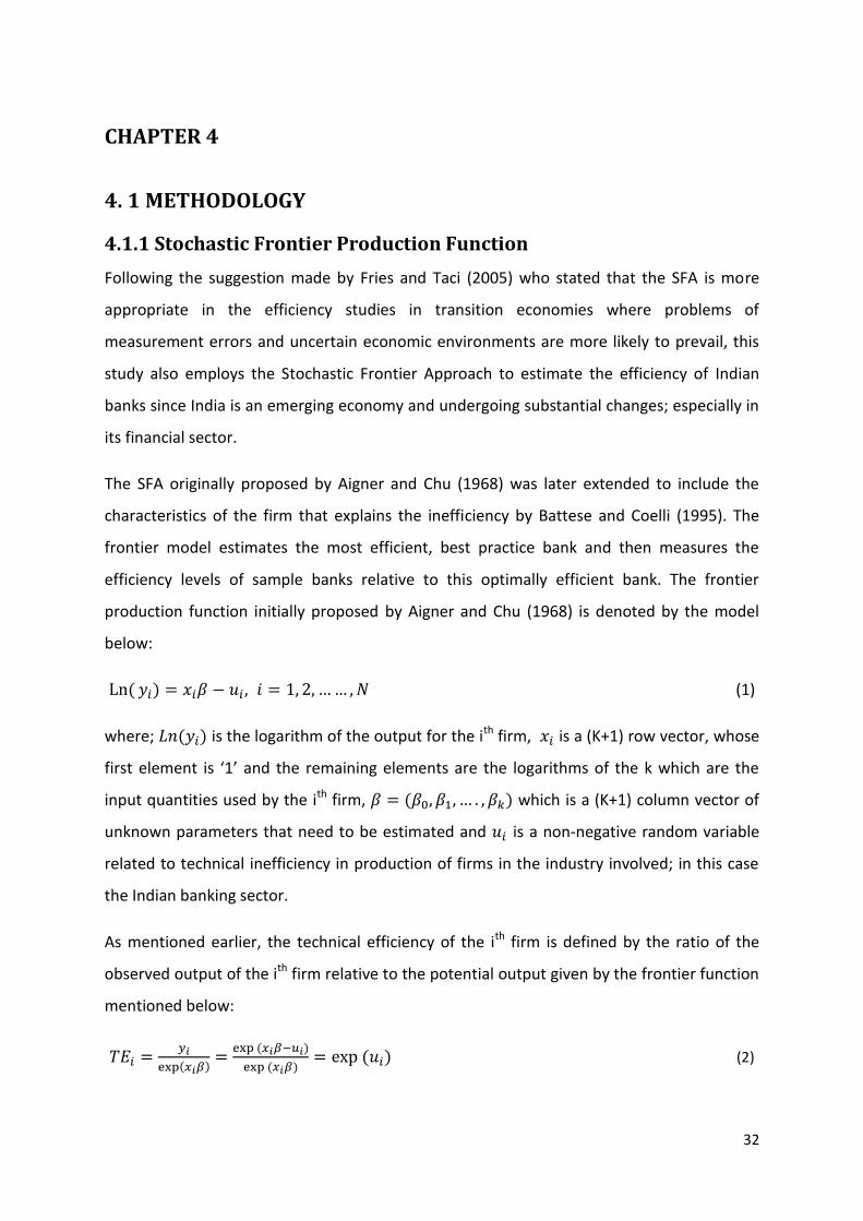
The SFA originally proposed by Aigner and Chu (1968) was later extended to include the
characteristics of the firm that explains the inefficiency by Battese and Coelli (1995). The
frontier model estimates the most efficient, best practice bank and then measures the
efficiency levels of sample banks relative to this optimally efficient bank. The frontier
production function initially proposed by Aigner and Chu (1968) is denoted by the model
below:
(1)
where; is the logarithm of the output for the ith firm, is a (K+1) row vector, whose
first element is ‘1’ and the remaining elements are the logarithms of the k which are the
input quantities used by the ith firm, which is a (K+1) column vector of
unknown parameters that need to be estimated and is a non-negative random variable
related to technical inefficiency in production of firms in the industry involved; in this case
the Indian banking sector.
As mentioned earlier, the technical efficiency of the ith firm is defined by the ratio of the
observed output of the ith firm relative to the potential output given by the frontier function
mentioned below:
(2)
33
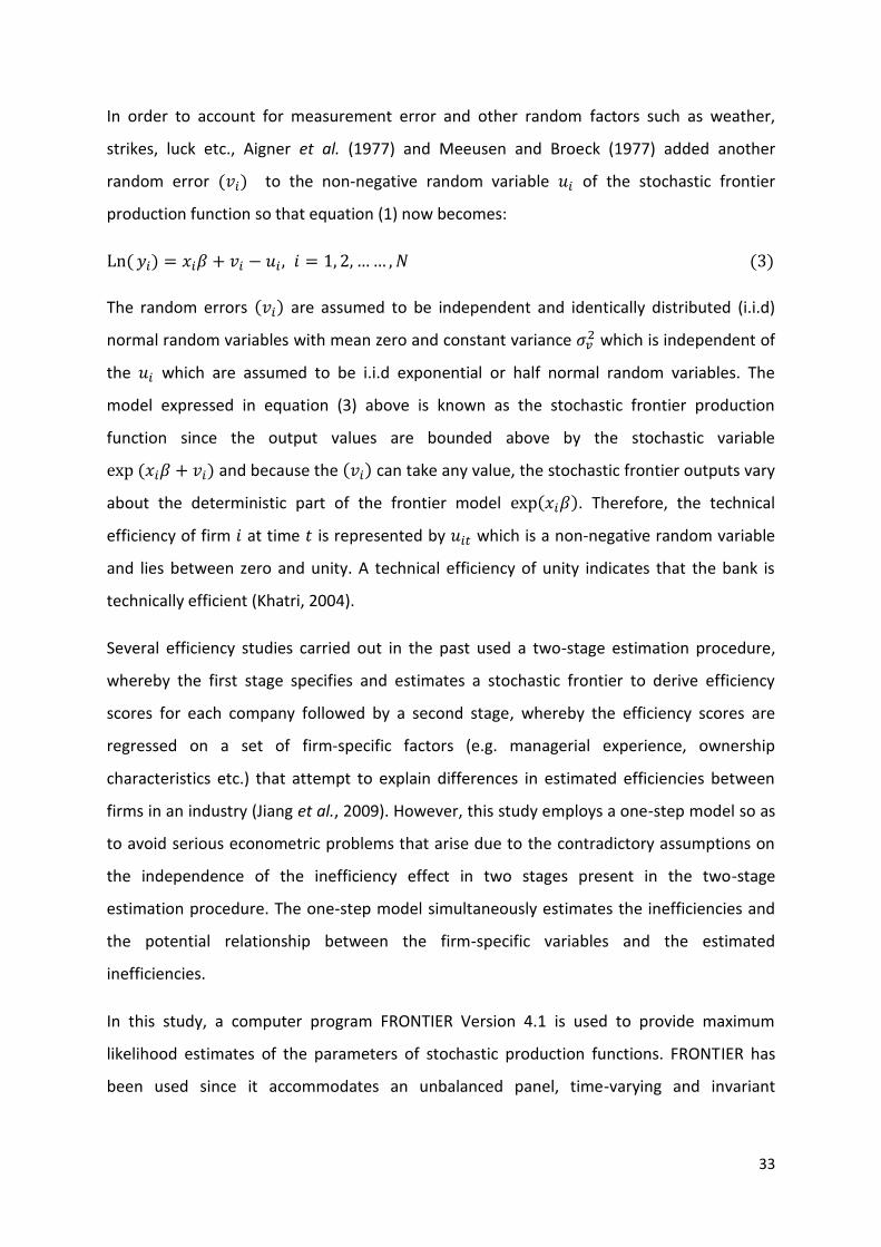
In order to account for measurement error and other random factors such as weather,
strikes, luck etc., Aigner et al. (1977) and Meeusen and Broeck (1977) added another
random error to the non-negative random variable of the stochastic frontier
production function so that equation (1) now becomes:
The random errors are assumed to be independent and identically distributed (i.i.d)
normal random variables with mean zero and constant variance which is independent of
the which are assumed to be i.i.d exponential or half normal random variables. The
model expressed in equation (3) above is known as the stochastic frontier production
function since the output values are bounded above by the stochastic variable
and because the can take any value, the stochastic frontier outputs vary
about the deterministic part of the frontier model . Therefore, the technical
efficiency of firm at time is represented by which is a non-negative random variable
and lies between zero and unity. A technical efficiency of unity indicates that the bank is
technically efficient (Khatri, 2004).
Several efficiency studies carried out in the past used a two-stage estimation procedure,
whereby the first stage specifies and estimates a stochastic frontier to derive efficiency
scores for each company followed by a second stage, whereby the efficiency scores are
regressed on a set of firm-specific factors (e.g. managerial experience, ownership
characteristics etc.) that attempt to explain differences in estimated efficiencies between
firms in an industry (Jiang et al., 2009). However, this study employs a one-step model so as
to avoid serious econometric problems that arise due to the contradictory assumptions on
the independence of the inefficiency effect in two stages present in the two-stage
estimation procedure. The one-step model simultaneously estimates the inefficiencies and
the potential relationship between the firm-specific variables and the estimated
inefficiencies.
In this study, a computer program FRONTIER Version 4.1 is used to provide maximum
likelihood estimates of the parameters of stochastic production functions. FRONTIER has
been used since it accommodates an unbalanced panel, time-varying and invariant

34
efficiencies, half-normal and truncated normal distributions and functional forms which
consist of the dependent variable in logged or original units (Coelli, 1994).
Previous empirical studies have increasingly applied the distance function approach whose
main advantage is that it accommodates multiple-outputs and multiple-inputs production
technology. Additionally, when price information is unreliable or unavailable and/or
behaviour assumptions of cost minimisation or profit maximisation are inappropriate, the
distance function approach is an ideal approach as compared to the traditional dual
approach which does not take into account of multiple-outputs and multiple-inputs when
estimating a cost and/or profit function (Cuesta and Orea, 2002; Coelli and Perelman, 2000).
Therefore, this study employs a stochastic output distance function which was initially
introduced by Shephard (1970) to accommodate the multi-product nature of the Indian
financial sector by using simply the quantities as data. Since the Indian economy consists of
a substantial gap between the rich and the poor, it is difficult to come to a conclusion as to
whether Indian banks achieve cost minimisation or profit maximisation. Therefore, the most
suitable way to deal with this situation is to use the distance function approach.
Therefore, based on the common definition of production technology that converts inputs
into outputs, the output distance function is defined by the following output set P(x).
will be less than or equal to one if the output vector, y, is an element of the
feasible production set of P(x).
where is the scalar ‘distance’ by which the output vector can be deflated. According to
Sturm and Williams (2008), an empirical representation of the stochastic output distance
function in a translog form for i firms producing M outputs using K inputs is shown by
equation (5) below:
35
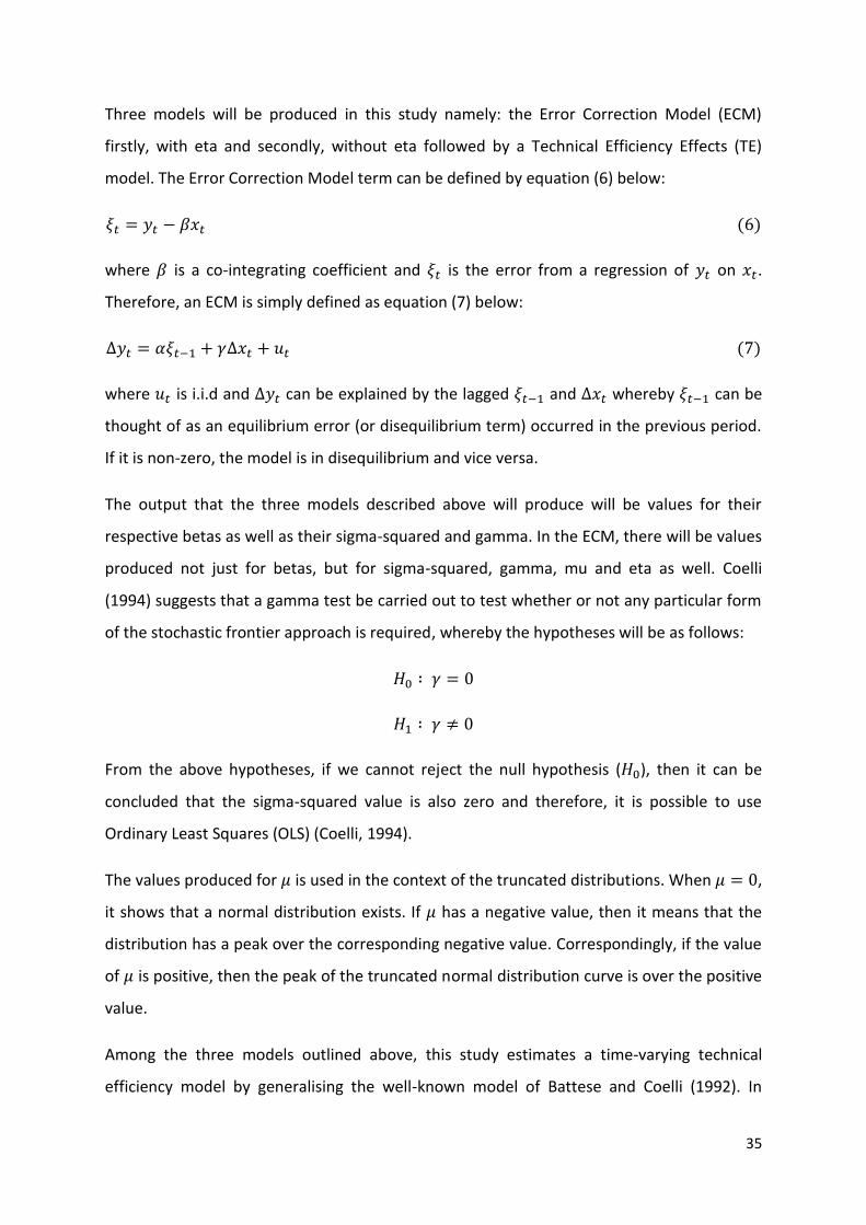
Three models will be produced in this study namely: the Error Correction Model (ECM)
firstly, with eta and secondly, without eta followed by a Technical Efficiency Effects (TE)
model. The Error Correction Model term can be defined by equation (6) below:
where is a co-integrating coefficient and is the error from a regression of on .
Therefore, an ECM is simply defined as equation (7) below:
where is i.i.d and can be explained by the lagged and whereby can be
thought of as an equilibrium error (or disequilibrium term) occurred in the previous period.
If it is non-zero, the model is in disequilibrium and vice versa.
The output that the three models described above will produce will be values for their
respective betas as well as their sigma-squared and gamma. In the ECM, there will be values
produced not just for betas, but for sigma-squared, gamma, mu and eta as well. Coelli
(1994) suggests that a gamma test be carried out to test whether or not any particular form
of the stochastic frontier approach is required, whereby the hypotheses will be as follows:
From the above hypotheses, if we cannot reject the null hypothesis ( ), then it can be
concluded that the sigma-squared value is also zero and therefore, it is possible to use
Ordinary Least Squares (OLS) (Coelli, 1994).
The values produced for is used in the context of the truncated distributions. When ,
it shows that a normal distribution exists. If has a negative value, then it means that the
distribution has a peak over the corresponding negative value. Correspondingly, if the value
of is positive, then the peak of the truncated normal distribution curve is over the positive
value.
Among the three models outlined above, this study estimates a time-varying technical
efficiency model by generalising the well-known model of Battese and Coelli (1992). In

36
contrast to Battese and Coelli (1992), this paper relaxes the monotonicity of the temporal
variation pattern of the efficiency term. Since technical efficiency is assumed to vary with
time in parametric form, it is possible to test whether the technical efficiency evolution of
the Indian banks is statistically significant. Therefore, to carry out the above comparison,
there are two ECM performed; the first with eta and the second without eta. Setting
provides a time invariant model. In the case where , the inefficiency term
is always decreasing with time, whereas if , it implies that is always increasing
with time. Therefore, performing an ECM with and without eta allows us to evaluate
whether time has any effect on the efficiency levels of Indian banks.
The last model called the TE model by Battese and Coelli (1995) can be expressed by
equation (8) below:
where , , and are defined as earlier and , where and
is a vector of firm-specific variables which may influence the firms’ efficiency (Herrero
and Pascoe, 2002).
4.1.2 Profitability Model
The profitability model is one that will reveal the factors that influence the profits and
margins of Indian banks. A Fixed Effects (FE) panel data model has been utilised to evaluate
the effects of nine determinants of bank profitability in India. The FE model aids in
controlling for bank-specific effects across periods. It allows for the endogeneity between
the variables and the unobserved heterogeneity. The general model is presented in
equation (9) below:
where and denote the individual bank and time period respectively, is a
constant, is the coefficient to be estimated for each factor, is an error term, refers to
the dependent variable, is a vector captured from the internal factors of the bank and
is a vector captured from the external factors of a bank.
37
where and denote the individual bank and time period respectively, is a
constant, is the coefficient to be estimated for each factor and is the residual that
contains unobserved determinants and errors.
4.2 DATA
Considering the evolutionary process of the Indian banking sector and the organisational
structure of banks, Indian banks are classified into two main groups; scheduled commercial
banks and scheduled cooperative banks which have three sub-groups each; public sector
banks (27 banks), private sector banks (22 banks) and foreign banks (41 banks) under the
former category and regional rural banks (82 banks), urban cooperative banks (52 banks)
and state cooperative banks (16 banks) in the latter category.
This study collects data for 11 years from 2001 to 2011. The sample period includes several
reforms such as enacting new laws or amending old legislations so as to keep up to date
with the changing circumstances; given that India is an emerging economy and has a fast
growing financial sector. Some of the changes that took place during the sample period
include: the Reserve Bank of India Act, 1934 being amended in 2006 to provide legality to
certain over-the-counter (OTC) derivative transactions and to give the Reserve Bank explicit
regulatory powers over derivatives and money market instruments. The State Bank of India
(Subsidiary Banks) Act, 1959 was also amended in 2007 to facilitate enhancement of capital,
raise resources from the market and raise capital through rights issue. This shows
movement towards a future objective of stipulating the capital requirements and other
quantitative parameters from time to time, instead of the Reserve Bank simply prescribing
quantitative limits in the respective Acts. Additionally, efforts are being made to converge
the Indian Accounting Standards (IAS) with the International Financial Reporting Standards
(IFRS), therefore, some of the changes that have been made are to progress towards
achieving this goal in the future (Reserve Bank of India, 2013).
The sample contains 154 observations in an unbalanced panel with 18 banks being the
maximum number of banks in the panel. The main data source is the monthly updated
BankScope Bureau Van Dijk which is an international database of a large number of banks
38
around the world. Since the quality of data in India is questionable, other complementary
data sources such as the Reserve Bank of India, Indian Banks’ Association and Indexmundi
India have been used.
Empirical studies indicate that efficiency estimates can be sensitive to the specification of
inputs and outputs. This paper employs three input variables (x1, x2 and x3) and three output
variables (y1, y2 and y3). Input variables include Total Interest Expense (TIE), Other Operating
Expense (OOE) and Deposit and Short-term Funding (DSF), whereas output variables include
Loans (LOANS), Net Interest Income (NETIR) and Other Operating Income (OOINC).
After getting the raw data from BankScope, all unconsolidated bank data was deleted and
missing values were replaced with ‘0’ since FRONTIER 4.1 only accepts integer values when
estimating bank efficiencies. All input and output variables were then deflated by their
corresponding years’ GDP deflators which were obtained from Indexmundi India. Banks
which did not have data available for most or all of the variables were then deleted leading
to an unbalanced panel of data. Missing values of ‘0’ that existed in the deflated Deposits
and Short-term Funding (DDSF) was replaced with ‘100’. Deflated equity (DEQUITY), net
interest income (DNETIR), net gains on trading and derivatives (DNETT), net gains (losses) on
assets at fair value through income statement (DNETINC), net fees and commission
(DNETFEE), loan loss provision (DLLP) and total non-interest operating income (DTNIOINC)
had some negative values and therefore, logarithms of these values could not be found. To
deal with this situation, these variables were scaled up to make them positive, but having no
effect on the rest of the values in the respective column since this rule applied to the entire
column of data. All input and output variables have been mean corrected, meaning that all
data are normalised by their geometric sample mean.
For the profitability model, Return on Average Equity (ROAE) was chosen as a performance
measure to be the proxy for bank profitability in India and therefore, was selected as the
dependant variable. ROAE is calculated by dividing the net income by the total average
equity. It shows the returns generated from the bank's total equity and reveals the
efficiency with which a bank can internally generate profit.

39
In general, the literature on bank performance mentioned that the profitability
determinants can be classified into two main categories, namely the internal determinants
(i.e. those factors that are influenced by the bank's management decisions and policy
objectives) and the external determinants (i.e. economic and industry conditions). The
variables chosen to measure the performance of banks along with those chosen to test the
factors that affect it are presented in Table 2 and discussed below.
Table 2: Explanatory Variables and Expected Signs
4.2.1 Internal Determinants
The primary method of evaluating internal performance of banks is by analysing accounting
data in the form of financial ratios. Financial ratios provide a greater understanding of bank
performance since they are constructed from bank’s financial statements.
Many empirical studies such as Kosmidou et al. (2005), Kosmidou (2008), Pasiouras and
Kosmidou (2007) and Alexiou and Sofoklis (2009) have used the Equity to Total Assets (ETA)
ratio and consider it to be one of the most important bank-specific determinants. ETA
provides a direct view of the banks' capital structure and the average soundness and
average safety of the financial institutions (Vong and Chan, 2009). A higher ETA ratio shows
that banks have more internal sources of finance as compared to external sources, which in
turn results in lower bankruptcy risk since there are fewer loans to pay back. Therefore, a
positive and significant relationship is expected between ETA and the Indian banks'
profitability.
40
This paper uses a Cost to Income (COSTINCOME) ratio so as to measure the cost efficiency
of Indian banks. In this case, costs are referred to as banks' overhead costs such as salaries
and wages, office rental, stationary expenses, advertisement expenses and other
miscellaneous expenses. The COSTINCOME ratio indicates how operational costs change
with respect to operating income. A high COSTINCOME ratio shows that banks cannot
efficiently manage its operations and therefore, the findings of previous literatures imply
that the relationship between the COSTINCOME ratio and bank profitability is negative
(Alexiou and Sofoklis, 2009).
The liquidity of banks is measured by the Net Loans to Total Assets (NLTA) ratio which
presents the percentage of assets that are financed with loans. Loans are the largest
segment of interest bearing assets and are expected to have a positive relationship with
bank performance (Vong and Chan, 2009). The higher the NLTA ratio, the lower the bank's
liquidity, however, previous empirical studies suggest that this leads to a high profitability
(Bourke, 1989; Trujillo-Ponce, 2012). However, in some cases where banks are rapidly
increasing their loan books, this may lead to higher costs being incurred for their funding
requirements which in turn could lead to a negative impact on profitability (Vong and Chan,
2009).
The Loans to Total Customer Deposits (LTCD) ratio is a commonly used statistic for
evaluating bank's liquidity position by dividing the banks' total loans by its total customer
deposits. If the LTCD is too high then it shows that the banks may not have enough liquidity
to cover for any unforeseen fund requirements, whereas if the ratio is too low, then it
means that banks may not be earning as much as they could be (Ongore and Kusa, 2013).
According to The World Bank (2013), a bank’s Capital to Assets (CTA) ratio is the ratio of
bank capital and reserves to total assets. The numerator consists of funds contributed by
owners, retained earnings, general and special reserves, provisions and valuation
adjustments. Capital includes tier 1 capital (paid-up shares and common stock) and
regulatory capital which includes various specified types of sub-ordinated debt instruments
that do not need to be repaid if the funds are required to maintain minimum capital levels
(tier 2 and tier 3 capital). The denominator includes both non-financial and financial assets.
According to Berger (1995), a higher capital level leads to higher profitability since banks can
41
easily adhere to regulatory capital standards so that excess capital can be loaned to
borrowers. This ratio reveals capital adequacy and should indicate the general safety and
soundness of the bank (Gul et al., 2011). It shows to what extent banks can withstand losses
and handle risk exposure for shareholders. Scholars such as Hassan and Bashir (2003) and
Bourke (1989) have found a positive relationship between CTA and bank profitability since
they deem that well-capitalised banks are less risky and more profitable.
Many researchers believe that bank Size (SIZE) has a non-linear relationship with
profitability. Athanasoglou et al. (2008), state that in the case of small-sized banks, the
profitability of these banks will increase along with an increase in size. However, when
banks are large to some extent, the size effect on profitability will become negative because
of bureaucracy. Therefore, the result of the size effect in this study is expected to be
positive.
4.2.2 External Determinants
In order to isolate the effects of bank characteristics on performance, it is necessary to also
include in the study other factors which may also have an influence on determining bank
performance.
So as to include a proxy for economic growth, the Gross Domestic Product Growth Rate
(GDPGR) is included in the model. It is calculated as the percentage change in the GDP in
each year. According to Bashir (2003), profitability of banks can be enhanced due to
economic growth due to the increased demand for financial transactions; meaning that
household and businesses tend to demand for loans. An increase in the demand for financial
services is then associated with an upward movement in the bank’s cash flows, profits and
non-interest earnings. Furthermore, fewer loans would be defaulted during strong
economic conditions. Kosmidou et al. (2005) also state that during a period of economic
growth, banks are less prudent in their lending since they assume that fewer borrowers will
default on their loans and can therefore, improve their income as more loans are issued.
Hence, academics such as Kosmidou et al. (2005), Pasiouras and Kosmidou (2007),
Kosmidou (2008) and Alexiou and Sofoklis (2009) assert that GDPGR should have a positive
influence on bank profitability. Therefore, this paper also expects that there is a positive
relationship between GDPGR and the performance of Indian banks.
42
Inflation (INFLATION) is the rate at which the general level of prices for goods and services is
rising and subsequently leads to the purchasing power to fall meaning that one unit of a
currency can buy less number of goods and services. So as to maintain the level of inflation
at a relatively stable level, the central bank adjusts the interest rate. Therefore, a rise in
inflation would lead to an increase in the interest rate which is likely to result in higher
profits for banks. According to scholars such as Demirgiic-Kunt and Huizinga (1999),
Mamatzakis and Remoundos (2003), Pasiouras and Kosmidou (2007), Athanasoglou et al.
(2008) and Alexiou and Sofoklis (2009), if inflation is correctly anticipated, then it can
improve bank profitability.
Market Capitalisation (MARKETCAP) is used as a proxy for stock market development. It
measures the ability of the stock market to allocate capital to investment projects and it
shows the capability to provide substantial opportunities for risk diversification to investors.
Well-developed stock markets would enhance the performance of banks since this would
allow banks to trade their equity shares, thereby increasing their capital requirements.
Higher capital would transform into higher earnings to the customers and shareholders
(Berger, 1995). Additionally, Demirguc-Kunt and Maksimovic (1996) state that stock markets
provide banks with liquidity and with opportunities to diversify their portfolios.
After finalising the above variables, equation (10) above now becomes:
where the coefficients will be estimated for each factor and is the residual that contains
unobserved determinants and errors.
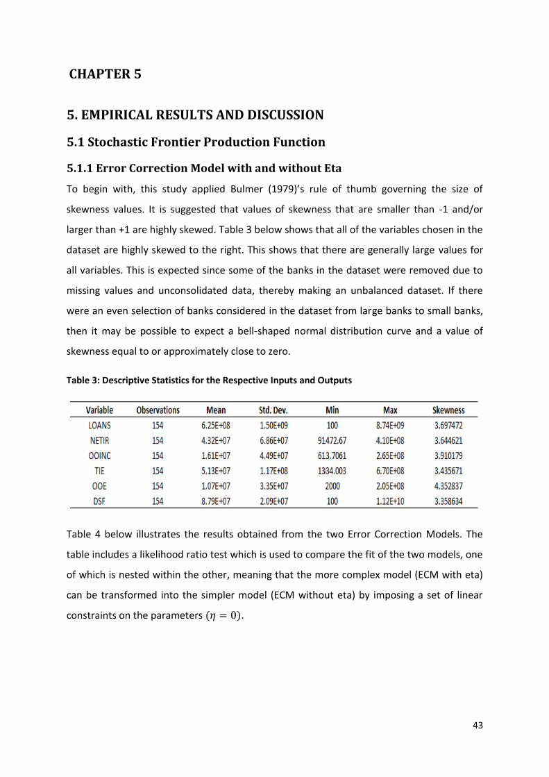
43
CHAPTER 5
5. EMPIRICAL RESULTS AND DISCUSSION
5.1 Stochastic Frontier Production Function
5.1.1 Error Correction Model with and without Eta
To begin with, this study applied Bulmer (1979)’s rule of thumb governing the size of
skewness values. It is suggested that values of skewness that are smaller than -1 and/or
larger than +1 are highly skewed. Table 3 below shows that all of the variables chosen in the
dataset are highly skewed to the right. This shows that there are generally large values for
all variables. This is expected since some of the banks in the dataset were removed due to
missing values and unconsolidated data, thereby making an unbalanced dataset. If there
were an even selection of banks considered in the dataset from large banks to small banks,
then it may be possible to expect a bell-shaped normal distribution curve and a value of
skewness equal to or approximately close to zero.
Table 3: Descriptive Statistics for the Respective Inputs and Outputs
Table 4 below illustrates the results obtained from the two Error Correction Models. The
table includes a likelihood ratio test which is used to compare the fit of the two models, one
of which is nested within the other, meaning that the more complex model (ECM with eta)
can be transformed into the simpler model (ECM without eta) by imposing a set of linear
constraints on the parameters .
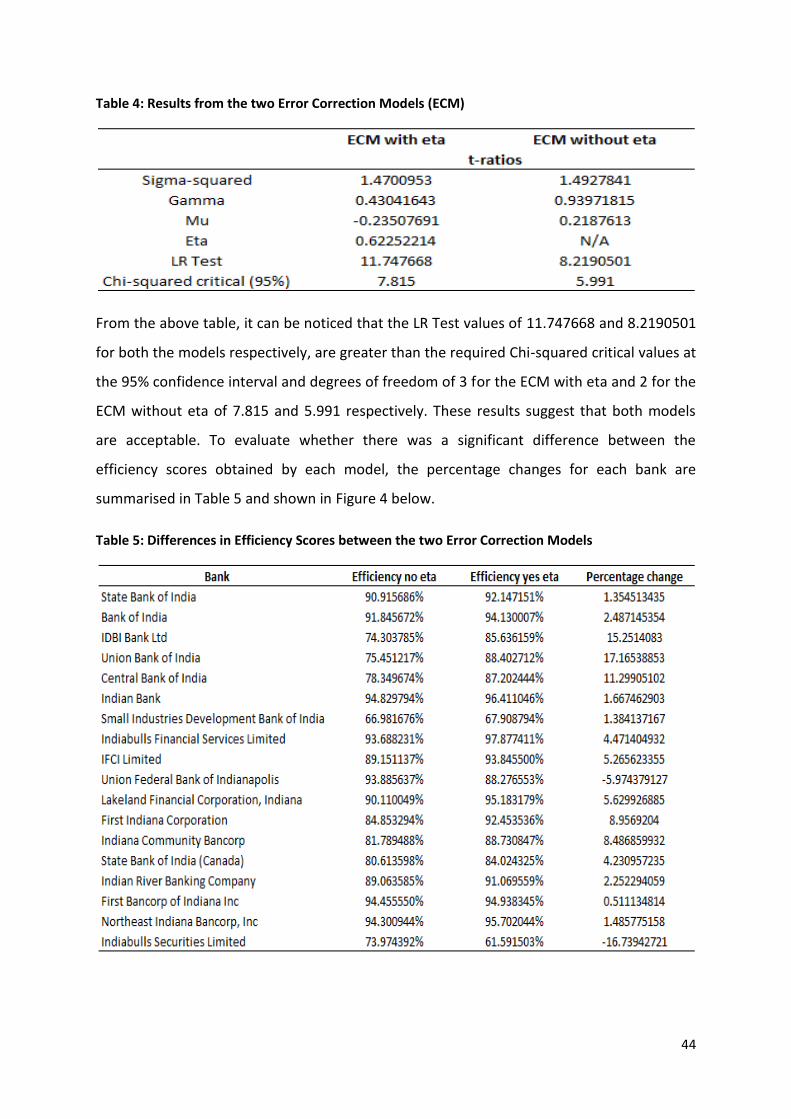
44
Table 4: Results from the two Error Correction Models (ECM)
From the above table, it can be noticed that the LR Test values of 11.747668 and 8.2190501
for both the models respectively, are greater than the required Chi-squared critical values at
the 95% confidence interval and degrees of freedom of 3 for the ECM with eta and 2 for the
ECM without eta of 7.815 and 5.991 respectively. These results suggest that both models
are acceptable. To evaluate whether there was a significant difference between the
efficiency scores obtained by each model, the percentage changes for each bank are
summarised in Table 5 and shown in Figure 4 below.
Table 5: Differences in Efficiency Scores between the two Error Correction Models

45
Figure 4: Efficiency Scores Obtained from ECM with and without Eta
0%
20%
40%
60%
80%
100%
120%
Effi
cie
ncy
Sco
re (
%)
Bank
Efficiency Scores Obtained From ECM With and Without Eta
Efficiency no eta
Efficiency yes eta
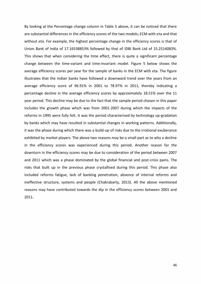
46
By looking at the Percentage change column in Table 5 above, it can be noticed that there
are substantial differences in the efficiency scores of the two models; ECM with eta and that
without eta. For example, the highest percentage change in the efficiency scores is that of
Union Bank of India of 17.16538853% followed by that of IDBI Bank Ltd of 15.2514083%.
This shows that when considering the time effect, there is quite a significant percentage
change between the time-variant and time-invariant model. Figure 5 below shows the
average efficiency scores per year for the sample of banks in the ECM with eta. The figure
illustrates that the Indian banks have followed a downward trend over the years from an
average efficiency score of 96.91% in 2001 to 78.97% in 2011, thereby indicating a
percentage decline in the average efficiency scores by approximately 18.51% over the 11
year period. This decline may be due to the fact that the sample period chosen in this paper
includes the growth phase which was from 2001-2007 during which the impacts of the
reforms in 1995 were fully felt. It was the period characterised by technology up-gradation
by banks which may have resulted in substantial changes in working patterns. Additionally,
it was the phase during which there was a build-up of risks due to the irrational exuberance
exhibited by market players. The above two reasons may be a small part as to why a decline
in the efficiency scores was experienced during this period. Another reason for the
downturn in the efficiency scores may be due to consideration of the period between 2007
and 2011 which was a phase dominated by the global financial and post-crisis pains. The
risks that built up in the previous phase crystallised during this period. This phase also
included reforms fatigue, lack of banking penetration, absence of internal reforms and
ineffective structure, systems and people (Chakrabarty, 2013). All the above mentioned
reasons may have contributed towards the dip in the efficiency scores between 2001 and
2011.
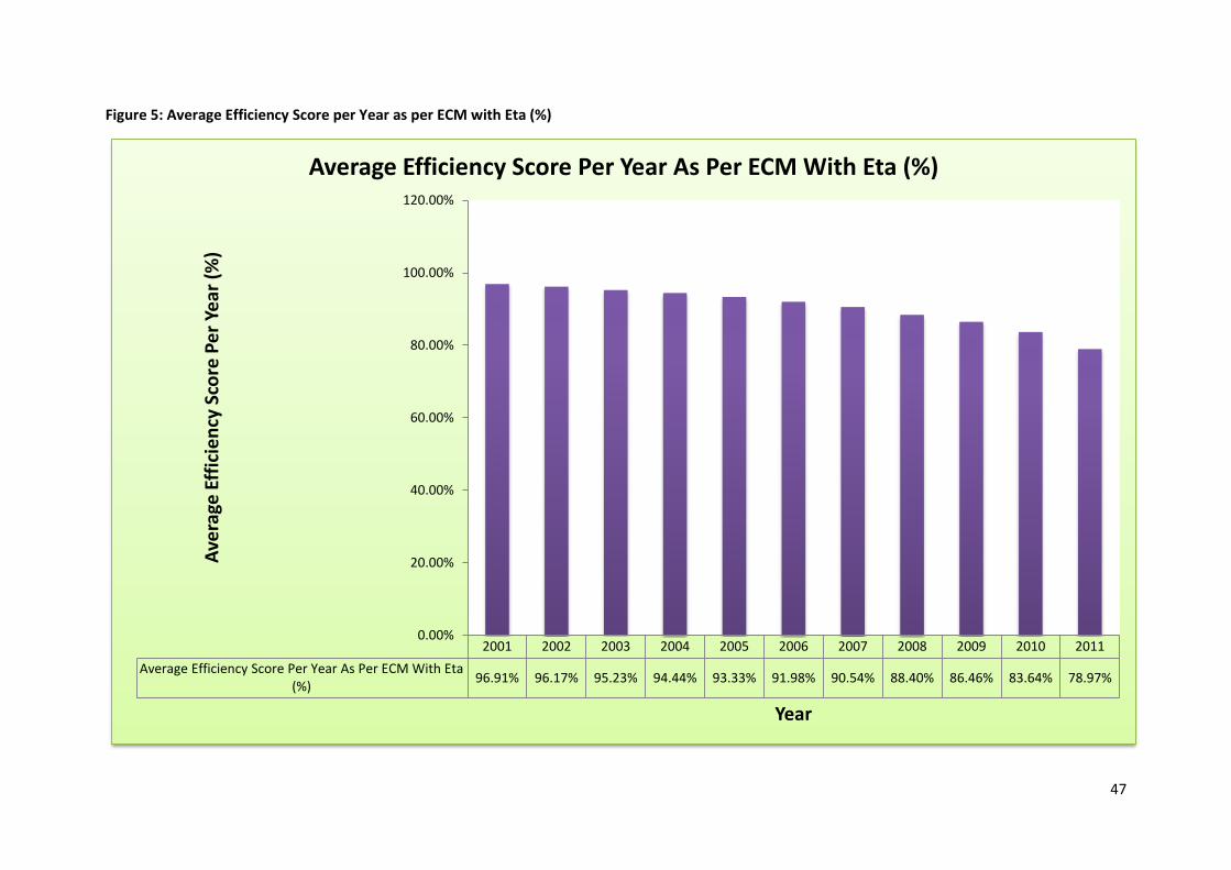
47
Figure 5: Average Efficiency Score per Year as per ECM with Eta (%)
2001 2002 2003 2004 2005 2006 2007 2008 2009 2010 2011
Average Efficiency Score Per Year As Per ECM With Eta (%)
96.91% 96.17% 95.23% 94.44% 93.33% 91.98% 90.54% 88.40% 86.46% 83.64% 78.97%
0.00%
20.00%
40.00%
60.00%
80.00%
100.00%
120.00% A
vera
ge E
ffic
ien
cy S
core
Pe
r Ye
ar (
%)
Year
Average Efficiency Score Per Year As Per ECM With Eta (%)
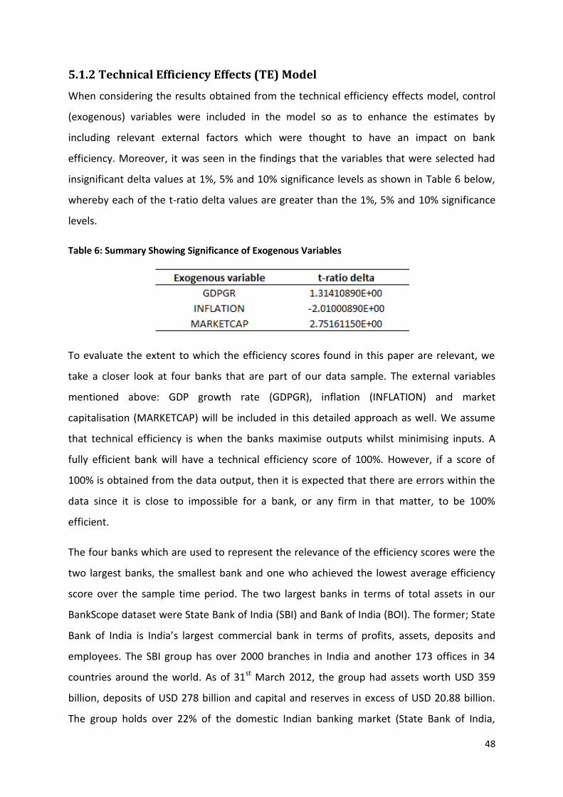
48
5.1.2 Technical Efficiency Effects (TE) Model
When considering the results obtained from the technical efficiency effects model, control
(exogenous) variables were included in the model so as to enhance the estimates by
including relevant external factors which were thought to have an impact on bank
efficiency. Moreover, it was seen in the findings that the variables that were selected had
insignificant delta values at 1%, 5% and 10% significance levels as shown in Table 6 below,
whereby each of the t-ratio delta values are greater than the 1%, 5% and 10% significance
levels.
Table 6: Summary Showing Significance of Exogenous Variables
To evaluate the extent to which the efficiency scores found in this paper are relevant, we
take a closer look at four banks that are part of our data sample. The external variables
mentioned above: GDP growth rate (GDPGR), inflation (INFLATION) and market
capitalisation (MARKETCAP) will be included in this detailed approach as well. We assume
that technical efficiency is when the banks maximise outputs whilst minimising inputs. A
fully efficient bank will have a technical efficiency score of 100%. However, if a score of
100% is obtained from the data output, then it is expected that there are errors within the
data since it is close to impossible for a bank, or any firm in that matter, to be 100%
efficient.
The four banks which are used to represent the relevance of the efficiency scores were the
two largest banks, the smallest bank and one who achieved the lowest average efficiency
score over the sample time period. The two largest banks in terms of total assets in our
BankScope dataset were State Bank of India (SBI) and Bank of India (BOI). The former; State
Bank of India is India’s largest commercial bank in terms of profits, assets, deposits and
employees. The SBI group has over 2000 branches in India and another 173 offices in 34
countries around the world. As of 31st March 2012, the group had assets worth USD 359
billion, deposits of USD 278 billion and capital and reserves in excess of USD 20.88 billion.
The group holds over 22% of the domestic Indian banking market (State Bank of India,
49
2013). The latter; Bank of India was founded in 1906 by a group of well-known businessmen
from Mumbai. In 1969, the bank was nationalised. Today, it is the fourth largest bank in
India with approximately USD 75.58 billion worth of total assets as of March 2012, 4322
branches in the country spread over all states or union territories and has overseas presence
in 20 foreign countries spread over 5 continents (Bank of India, 2013; Relbanks.com, 2013).
Since IFCI Limited (IFCI) was the smallest bank in the dataset with complete data for all the
11 years from 2001 to 2011, it is considered to be the smallest bank and therefore,
represents the third bank for this analysis.
When calculating the overall average efficiency scores over the 11 year period, it was found
that Small Industries Development Bank of India (SIDBI) was found to have the lowest
average efficiency score of 85.53%. Therefore, this bank was chosen to represent the fourth
bank in this analysis.
To show the performance of the above mentioned banks, the annual efficiency scores
obtained from the technical efficiency effects model in FRONTIER 4.1 can be shown in Figure
6 below.
So as to see the extent to which the findings corresponded to reality, we can see from the
figure below that the performance of Small Industries Development Bank of India
deteriorated from 2008 until 2010. Efficiency scores of State Bank of India, Bank of India and
IFCI Limited dipped for a relatively short period of time from 2009 to 2010. This downturn
may be due to the fact that the banks were feeling the after effects of the global financial
crisis which took place in 2007-2008. This may have been partly due to the loosening of
bank regulations so as to give borrowers loans imprudently and allow them some room
while the subprime housing chaos started in the USA. This resulted in more than 9% of all
loans being considered as bad debts. State Bank of India reported that 25% of its loans were
non-performing and that 13% of the total figure was allocated to the substantially indebted
banks (The Economist, 2013).
Additionally, according to a study carried out by Bhattacharyya and Chatri (2012), it was
found that during the period of 2001 and 2010, there were about 13 mergers and
acquisitions which had taken place. Evidence of the above statement can be shown by the
50
amalgamation of the SBI with State Bank of Saurashtra in 2008. These mergers and
acquisitions posed a threat of increased competition in the Indian banking sector which may
have led to the decline in the efficiency scores since the increased competitive pressure is
likely to have affected the profit margins and cost of intermediation of the banks. Cuesta
and Orea (2002) also found that the efficiency scores in their study declined immediately
after mergers had taken place in the Spanish banking sector.
Another reason for the drop in efficiency scores may be due to high capital requirements by
the Basel Committee which would have led to a buffer being set aside for the purpose of
unexpected losses. This means that the capital that would have been kept as buffer could
not be lent out and therefore, may have resulted in the efficiency of the banks decreasing.
The State Bank of India had a Tier 1 Capital of Rs. 76149 crores (approximately USD 11.8
billion) as at June 2009 (State Bank of India, 2009). Similarly, as at September 2010, Bank of
India had a Tier 1 Capital of Rs. 12641.32 crores (approximately USD 19.65 billion) (Bank of
India, 2009). These statistics show that quite a lot of capital is caught up due to the fact that
the banks need to provision for unexpected losses, thus may have had a negative effect on
the banks’ efficiency.
However, all the above mentioned factors seem to have had only a short-term effect on the
banks' efficiencies since from 2010, it can be seen that the efficiency scores of the four
banks follow an upward trend.
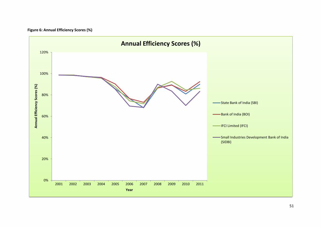
51
Figure 6: Annual Efficiency Scores (%)
0%
20%
40%
60%
80%
100%
120%
2001 2002 2003 2004 2005 2006 2007 2008 2009 2010 2011
An
nu
al E
ffic
ien
cy S
core
s (%
)
Year
Annual Efficiency Scores (%)
State Bank of India (SBI)
Bank of India (BOI)
IFCI Limited (IFCI)
Small Industries Development Bank of India (SIDBI)
52
5.2 Profitability Model
Table 7 below illustrates the findings obtained from the analysis of the Fixed Effects model.
It shows that all the p-values are greater than the 10% significance level showing that they
do not significantly have an impact on the profitability of the firm measured in terms of
ROAE in this paper. Most of the findings are contrary to the expectations that were made.
The Equity to Total Assets (ETA) ratio was expected to have a positive impact on ROAE.
However, the findings show that ETA has a negative influence on bank performance which is
in contrast to previous studies (Berger (1995); Demirgiic-Kunt and Huizinga (1999);
Staikouras and Wood (2003); Goddard et al. (2004); Kosmidou et al. (2005); Kosmidou
(2008)). This means that banks utilise greater external sources of finance (risky debt) rather
that internal sources of finance (equity), which means that Indian banks are more risky since
they are highly leveraged. Therefore, in the event of losses or liquidation, these banks are
considered relatively unsafe. Additionally, since the results show that the banks are highly
geared, this means that they may be incurring high costs of financing which may be another
reason for a decline in profitability. However, as mentioned above, the Equity to Total Assets
ratio is not considered as a significant measure of profitability, hence not having a major
influence on the ROAE.
The second internal variable considered in this study was the Cost to Income (COSTINCOME)
ratio. The results obtained were as expected; a negative relationship between COSTINCOME
and ROAE. This shows that an increase in overhead expenses reduces the profits of Indian
banks, but not significantly. The negative relationship between the Cost to Income ratio and
profitability is in line with that obtained by Alexiou and Sofoklis (2009) and Kosmidou et al.
(2005). Therefore, Indian banks may need to, to some degree, direct their attention to a
more efficient cost control measures so as to reduce their overhead costs which would
thereby have a positive impact on the profitability.
The Net Loans to Total Assets (NLTA) ratio is a liquidity ratio and was expected to have a
positive relationship with profitability. However, in this instance, an insignificant negative
relationship was found which was in contrast to the previous empirical studies by Bourke
(1989) and Trujillo-Ponce (2012). In this paper, it may be assumed that an increase in net
loans may lead to a fall in liquidity and a decline in profitability too. This may be due to the
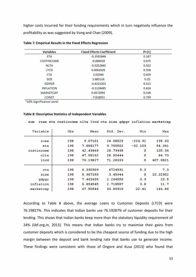
53
higher costs incurred for their funding requirements which in turn negatively influence the
profitability as was suggested by Vong and Chan (2009).
Table 7: Empirical Results in the Fixed Effects Regression
Table 8: Descriptive Statistics of Independent Variables
According to Table 8 above, the average Loans to Customer Deposits (LTCD) were
76.19827%. This indicates that Indian banks use 76.19287% of customer deposits for their
lending. This shows that Indian banks keep more than the statutory liquidity requirement of
24% (iibf.org.in, 2013). This means that Indian banks try to maximise their gains from
customer deposits which is considered to be the cheapest source of funding due to the high
margin between the deposit and bank lending rate that banks use to generate income.
These findings were consistent with those of Ongore and Kusa (2013) who found that
54
Kenyan banks utilised 77.50% of their customer deposits for lending. However, in this paper
this explanatory variable is not regarded as significant to influence profitability since the p-
value obtained from the Fixed Effects model as shown in Table 7 is greater than the 10%
significance level, thereby concluding that LTCD do not have a significant relationship with
ROAE.
The Capital to Assets (CTA) ratio presented results as those projected. A positive connection
existed between CTA and ROAE which shows that well capitalised banks represent sound
banks due to capital adequacy. However, as mentioned above, the ratio did not significantly
affect the profitability of Indian banks.
The effect of bank size (SIZE) on profitability was in line with the expectation that the size
effect has a positive influence on ROAE. The positive coefficient suggests that larger banks
tend to earn higher profits, to some extent, as compared to smaller banks. This may be due
to economies of scale which leads to lower average costs, thus an increase in the
profitability. These findings were consistent with those of Smirlock (1985) who also found a
positive relation. However, unlike our case, their relationship was significant. This may be
because small-sized banks usually try to grow faster, even if it means sacrificing profit in the
short term. Additionally, some of the banks may have an objective of gaining market share
even if it means forgoing profits. Therefore, the above suggests that the size variable does
not have a substantial influence on bank performance.
The impact of the indicators of macroeconomic conditions on ROAE is insignificant in all
cases. In the case of GDP growth (GDPGR), a negative correlation was found with
profitability. This was in contrast to what was expected. The insignificance of this
macroeconomic variable to bank performance may be due to the relatively small average
GDP growth of 7.463636% as shown in Table 8 above.
According to Table 7, inflation (INFLATION) seemed to bring a higher increase in costs than
revenues as the negative relation between INFLATION and ROAE indicates. The reason for
this may be that an increase in the general price level would make consumers reluctant from
spending which means they would borrow less and save more. Therefore, for the banks, this
means that the number of loans would fall and customer deposits may rise. Due to the fall in
55
loans, this may have a negative impact on bank profitability. The same findings were
obtained by Kosmidou et al. (2007) in the case of foreign banks in the European Union.
Market Capitalisation was used as a proxy of stock market development. A positive
correlation was found between the market capitalisation and the profitability of Indian
banks which was anticipated. This means that as the stock market enlarges, more
information is available and therefore, leads to an increase in the number of potential
customers to banks. This makes identification and monitoring of borrowers easier and
therefore, results in an increase in bank activity and profitability. These findings are similar
to those of Naceur (2003) who examined the profitability of the Tunisian banking sector.
56
CHAPTER 6
6.1 CONCLUSION
The liberalisation, growth and globalisation of emerging economies such as China and India
have attracted substantial sources of interest from researchers. Therefore, this paper
applied the Stochastic Frontier Approach (SFA) to measure the efficiency of Indian banks
using 3 models - the Error Correction Model (ECM), with and without eta, and the Technical
Efficiency Effects model - for an unbalanced panel of 18 Indian banks (154 observations) over
the period 2001 to 2011. The study further attempted to identify the determinants of the
profitability of Indian banks using Return on Average Equity (ROAE) as a measure of
profitability.
Empirical evidence from the ECM without eta demonstrated a very high mean efficiency
score of 84.92%. Similarly, the average efficiency score presented by the ECM with eta was
90.45%. However, there was quite a substantial difference between the efficiency scores
depicted by both the models. This showed that the time factor in the time-variant model
(ECM with eta) did have an influence on the efficiency of Indian banks. The third model, the
Technical Efficiency Effects model, included exogenous factors which were thought to have
an impact on the banks' efficiency. These include the GDP growth rate (GDPGR), Inflation
(INFLATION) and Market Capitalisation (MARKETCAP). However, when the data was run on
FRONTIER 4.1, the delta values obtained were all greater than the 1%, 5% and 10%
significance levels, meaning that the control variables did not have any significant impact on
bank efficiencies. A mean efficiency score in the TE model was 86.94% which is also a
relatively high score like in the case of the other two models.
The same exogenous variables listed above, together with financial ratios such as Equity to
Total Assets (ETA) ratio, Cost to Income (COSTINCOME) ratio, Net Loans to Total Assets
(NLTA) ratio, Loans to Customer Deposits (LTCD) ratio, and Capital to Total Assets (CTA) ratio
were regressed as determinants of ROAE in the profitability model. However, like in the case
of the Technical Efficiency Effects model, the above variables also had no influence on the
profitability of the banks in the sample.
57
To get a fair understanding as to whether the findings of this study were realistic, four banks
were chosen for further analysis: the two largest banks (State Bank of India and Bank of
India), the smallest bank with data available for all the 11 years during which this study
focused on (IFCI Limited) and lastly, the least efficient bank (Small Industries Development
Bank of India). The findings did seem to reflect reality since, from 2008 onwards, a
downward trend was seen in the efficiency scores of Small Industries Development Bank of
India from 2008 to 2010. Moreover, the other three banks' efficiency scores dipped from
2009 to 2010. SBI's efficiency scores dropped from 89.46% in 2009 to 80.81% in 2010. Bank
of India's scores dipped from 89.23% in 2009 to 83.28% in 2010. IFCI Limited's scores fell
from 92.80% in 2009 to 84.63% in 2010. Lastly, Small Industries Development Bank of India
felt the biggest plunge in efficiency scores from 90.08% in 2008 to 70.24% in 2010. All the
above may have been due to the after effects of the global financial crisis, mergers and
acquisitions that took place between 2001 and 2010 and increasing capital requirements
from the Basel Committee. However, since the efficiency scores of all four banks began to
follow an upward trend from 2010, it can be seen that they have recovered in a short period
of time.
6.2 LIMITATIONS AND SCOPE FOR FURTHER RESEARCH
The findings of this study could be subject to a few limitations which could be dealt with by
further research. Firstly, a sample period of only 11 years has been considered in this study,
which may have ignored some phases such as the pre- and post-liberalisation periods so as
to examine whether the reforms actually had a positive or negative impact on the efficiency
of Indian banks. Additionally, ownership was not considered in this study. Grouping banks
according to public, private and foreign ownerships may have given a better understanding
as to which ownership group is more inefficient. Another aspect which was thought to have
an influence on the inefficiencies from 2008 onwards was mergers and acquisitions.
Therefore, evaluating whether mergers and acquisitions did play a role in deteriorating the
efficiency of Indian banks will give us some certainty into this aspect. Lastly, since the
inefficiencies do exist in the Indian banking sector, policy makers and managers of banks
should focus on the internal factors, since the efficiencies lie within the banks. Hence,

58
recommendations and solutions from the regulators and managerial point of view may
improve the overall level of efficiencies in the banking sector.
59
REFERENCES Aigner, D. and Chu, S. 1968. On Estimating The Industry Production Function. The American Economic
Review, 58 (4), pp. 826--839. [Accessed: 30 July 2013].
Aigner, D., Lovell, K. and Schmidt, P. 1977. Formulation And Estimation Of Stochastic Frontier
Models. Journal of Econometrics, (6), pp. 21-37. [Accessed: 30 July 2013].
Alexiou, C. and Sofoklis, V. 2009. Determinants Of Bank Profitability: Evidence From The Greek
Banking Sector. Ekonomski anali, 54 (182), pp. 93--118. [Accessed: 05 August 2013].
Athanasoglou, P., Brissimis, S. and Delis, M. 2008. Bank-Specific, Industry-Specific And
Macroeconomic Determinants Of Bank Profitability. Journal of international financial Markets,
Institutions and Money, 18 (2), pp. 121--136. [Accessed: 11 August 2013].
Bajpai, N. 2011. Global Financial Crisis, Its Impact On India And The Policy Response. pp. 3-12.
[Accessed: 24 July 2013].
Bank Economists' Conference. 2002. Strengthening Indian Banking and Finance: Progress and
Prospects. [online] Available at: http://www.bimaljalan.com/speech271202.html [Accessed: 14
August 2013].
Bank of India. 2013. History. [online] Available at:
http://www.bankofindia.co.in/english/history3.aspx [Accessed: 14 August 2013].
Bank of India. 2009. Basel II (Pillar 3) - Disclosures (Consolidated) March 2009. [online] Available at:
http://www.bankofindia.co.in/pdf/Basel_March09.pdf [Accessed: 14 August 2013].
Bashir, A. 2013. Determinants Of Profitability In Islamic Banks: Some Evidence From The Middle
East. Islamic Economic Studies, 11 (1), pp. 32-57. Available at:
http://www.irti.org/irj/go/km/docs/documents/IDBDevelopments/Internet/English/IRTI/CM/do
wnloads/IES_Articles/Vol%2011-
1..A%20H%20Bashsir..Determinants%20of%20Profitability..dp.pdf [Accessed: 11 August 2013].
Battese, G. and Coelli, T. 1995. A Model For Technical Inefficiency Effects In A Stochastic Frontier
Production Function For Panel Data. Empirical economics, 20 (2), pp. 325--332. [Accessed: 30
July 2013].
Battese, G. and Coelli, T. 1992. A Stochastic Frontier Production Function Incorporating a Model for
Technical Inefficiency Effects. [Accessed: 29 August 2013].
Battese, G. and Corra, G. 1977. Estimation Of A Production Frontier Model: With Application To The
Pastoral Zone Of Eastern Australia. Australian Journal of Agricultural and Resource Economics, 21
(3), pp. 169--179. [Accessed: 19 August 2013].
Bera, A. and Sharma, S. 1999. Estimating Production Uncertainty In Stochastic Frontier Production
Function Models. Journal of Productivity Analysis, 12 (3), pp. 187--210. [Accessed: 26 July 2013].
Berger, A. 1995. The Relationship Between Capital And Earnings In Banking. Journal of Money, Credit
and Banking, 27 (2), pp. 432--456. [Accessed: 05 August 2013].
Berger, A. and Humphrey, D. 1997. Efficiency Of Financial Institutions: International Survey And
Directions For Future Research. European journal of operational research, 98 (2), pp. 175--212.
Available at: http://knowledge.wharton.upenn.edu/papers/67.pdf [Accessed: 24 July 2013].

60
Berger, A., Clarke, G., Cull, R., Klapper, L. and Udell, G. 2005. Corporate Governance And Bank
Performance: A Joint Analysis Of The Static, Selection, And Dynamic Effects Of Domestic,
Foreign, And State Ownership. Journal of Banking \& Finance, 29 (8), pp. 2179--2221. [Accessed:
27 August 2013].
Bhattacharyya, A., Lovell, C. and Sahay, P. 2007. The Impact Of Liberalization On The Productive
Efficiency Of Indian Commercial Banks. European Journal of Operational Research, 98 pp. 332-
345. Available at: http://www.lib.ctgu.edu.cn:8080/wxcd/qw/284.pdf [Accessed: 26 July 2013].
Bhattacharyya, A., Lovell, C. and Sahay, P. 1997. The Impact Of Liberalization On The Productive
Efficiency Of Indian Commercial Banks. European Journal of operational research, 98 (2), pp.
332--345. Available at: http://www.sciencedirect.com/science/article/pii/S0377221796003517
[Accessed: 12 August 2013].
Bhattacharyya, S. and Chatri, A. 2012. Efficiency Of Indian Commercial Banks: The Post-Reform
Experience From Mergers & Acquisitions. [Accessed: 02 September 2013].
Bhaumik, S. and Dimova, R. 2004. How Important Is Ownership In A Market With Level Playing Field?:
The Indian Banking Sector Revisited. Journal of Comparative Economics, 32 (1), pp. 165--180.
[Accessed: 22 August 2013].
Bourke, P. 1989. Concentration And Other Determinants Of Bank Profitability In Europe, North
America And Australia. Journal of Banking & Finance, 13 (1), pp. 65--79. [Accessed: 05 August
2013].
Bulmer, M. 1979. Principles Of Statistics. New York: Dover Publications.
Casu, B. and Molyneux, P. 2000. A Comparative Study Of Efficiency In European Banking. Applied
Economics, 35 (17), pp. 1865--1876. [Accessed: 25 August 2013].
Chakrabarty, K. 2013. Productivity Trends In Indian Banking In The Post Reform Period – Experience,
Issues And Future Challenges. pp. 01-22. Available at:
http://www.bis.org/review/r130815a.pdf?frames=0 [Accessed: 14 August 2013].
Coelli, T. 1994. FRONTIER Version 4.1 : A Computer Program For Stochastic Frontier Production And
Cost Function Estimation. Department of Econometrics, University of New England, Armidale,
NSW, [Accessed: 23 July 2013].
Coelli, T. and Perelman, S. 2000. Technical Efficiency Of European Railways: A Distance Function
Approach. Applied Economics, 32 (15), pp. 1967--1976. [Accessed: 03 August 2013].
Cuesta, R. and Orea, L. 2002. Mergers And Technical Efficiency In Spanish Savings Banks: A Stochastic
Distance Function Approach. Journal of Banking \& Finance, 26 (12), pp. 2231--2247. [Accessed:
03 August 2013].
D&B. 2013. Structure of Indian Banking System. [online] Available at:
http://www.dnb.co.in/bfsisectorinindia/BankC2.asp [Accessed: 26 July 2013].
Del Hoyo, J., Espino, D. and Toribio, R. 2004. Determination Of Technical Efficiency Of Fisheries By
Stochastic Frontier Models: A Case On The Gulf Of Cadiz (Spain). Journal of Marine Science, 61
pp. 416-421. [Accessed: 29 July 2013].
Demir, N., Mahmud, S. and Babuscu, S. 2005. The Technical Inefficiency Effects Of Turkish Banks
After Financial Liberalization. The Developing Economies, 43 (3), pp. 396--411. Available at:
61
http://onlinelibrary.wiley.com/doi/10.1111/j.1746-1049.2005.tb00951.x/pdf [Accessed: 18 July
2013].
Demirgicc-Kunt, A. and Huizinga, H. 1999. Determinants Of Commercial Bank Interest Margins And
Profitability: Some International Evidence. The World Bank Economic Review, 13 (2), pp. 379--
408. [Accessed: 06 August 2013].
Demirgicc-Kunt, A. and Maksimovic, V. 1996. Stock Market Development And Financing Choices Of
Firms. The World Bank Economic Review, 10 (2), pp. 341--369. [Accessed: 06 August 2013].
Deyoung, R. 1997. A Diagnostic Test For The Distribution-Free Efficiency Estimator: An Example Using
US Commercial Bank Data. European Journal of Operational Research, 98 (2), pp. 243--249.
Available at: http://www.sciencedirect.com/science/article/pii/S0377221796003451 [Accessed:
24 July 2013].
Dwivedi, A. and Charyulu, D. 2011. Efficiency Of Indian Banking Industry In The Post-Reform Era.
Indian Institute Of Management Ahmedabad, pp. 3-15. Available at:
http://www.iimahd.ernet.in/assets/snippets/workingpaperpdf/5467612052011-03-01.pdf
[Accessed: 24 July 2013].
Farrell, M. 1957. The Measurement Of Productive Efficiency. Journal of the Royal Statistical Society.
Series A (General), 120 (3), pp. 253--290. [Accessed: 19 August 2013].
Fries, S. and Taci, A. 2005. Cost Efficiency Of Banks In Transition: Evidence From 289 Banks In 15 Post-
Communist Countries. Journal of Banking \& Finance, 29 (1), pp. 55--81. [Accessed: 02 August
2013].
Goddard, J., Molyneux, P. and Wilson, J. 2004. The Profitability Of European Banks: A Cross-Sectional
And Dynamic Panel Analysis. The Manchester School, 72 (3), pp. 363--381. [Accessed: 02
September 2013].
Greene, W. 1990. A Gamma-Distributed Stochastic Frontier Model. Journal of econometrics, 46 (1),
pp. 141--163. Available at: http://pages.stern.nyu.edu/~wgreene/FrontierModeling/Reference-
Papers/Greene-JE1990-GammaFrontier_1.pdf [Accessed: 16 July 2013].
Gul, S., Irshad, F. and Zaman, K. 2011. Factors Affecting Bank Profitability in Pakistan. The Romanian
Economic Journal, 39 pp. 61--87. [Accessed: 10 August 2013].
Hassan, M. and Bashir, A. 2003. Determinants Of Islamic Banking Profitability. 16 [Accessed: 14
August 2013].
Herrero and Pascoe. 2002. Estimation Of Technical Efficiency: A Review Of Some Of The Stochastic
Frontier And DEA Software (CHEER V15 N1). [online] Available at:
http://www.economicsnetwork.ac.uk/cheer/ch15_1/dea.htm [Accessed: 03 August 2013].
Idialu, J. and Yomere, G. 2010. Stochastic Frontier Analysis Of The Efficiency Of Nigerian Banks. Indian
Journal of Economics and Business, 9 (1), pp. 75-86. [Accessed: 02 August 2013].
iibf.org.in. 2013. Cash Reserve Ratio (CRR) & Statutory Liquidity Ratio (SLR). [online] Available at:
http://www.iibf.org.in/documents/CRR-SLR.pdf [Accessed: 06 September 2013].
India Finance and Investment Guide. 2013. Reserve Bank of India (RBI): Functions Of RBI, Role of RBI.
[online] Available at: http://finance.indiamart.com/investment_in_india/rbi.html [Accessed: 23
July 2013].

62
Indian Banks' Association. 2013. Indian Banks' Association. [online] Available at:
http://www.iba.org.in/ [Accessed: 23 July 2013].
Jadhav. 2011. An Overview Of The Banking Sector. pp. 20-35. Available at:
http://shodhganga.inflibnet.ac.in/bitstream/10603/2031/10/10_chapter%201.pdf [Accessed: 23
July 2013].
Jiang, C., Yao, S. and Zhang, Z. 2009. The Effects Of Governance Changes On Bank Efficiency In China:
A Stochastic Distance Function Approach. China Economic Review, 20 (4), pp. 717--731. Available
at: http://www.sciencedirect.com/science/article/pii/S1043951X09000492 [Accessed: 02 August
2013].
Kablan, S. and Rine. 2007. Measuring Bank Efficiency In Developing Countries: The Case Of WAEMU
(West African Economic Monetary Union). African Economic Research Consortium, [Accessed: 22
August 2013].
Kamberoglou, N., Liapis, E., Simigiannis, G. and Tzamourani, P. 2004. Cost Efficiency In Greek Banking.
Bank of Greece WP, Available at: http://www.bankofgreece.gr/BogEkdoseis/Paper200409.pdf
[Accessed: 28 July 2013].
Khatri, D. 2004. Performance Of Indian Banks-Stochastic Frontier Approach. Available at:
http://papers.ssrn.com/sol3/papers.cfm?abstract_id=639801 [Accessed: 17 July 2013].
Kiyota, H. 2009. Efficiency Of Commercial Banks In Sub-Saharan Africa: A Comparative Analysis Of
Domestic And Foreign Banks. pp. 2-46. Available at:
http://www.csae.ox.ac.uk/conferences/2009-EDiA/papers/357-Kiyota.pdf [Accessed: 25 July
2013].
Kokkinou, D. and Geo, D. 2009. Stochastic Frontier Analysis: Empirical Evidence On Greek
Productivity. pp. 1-21. Available at:
http://www.lse.ac.uk/europeanInstitute/research/hellenicObservatory/pdf/4th_%20Symposium
/PAPERS_PPS/APPLIED_ECONOMICS/KOKKINOU.pdf [Accessed: 26 July 2013].
Kosmidou, K. 2008. The Determinants Of Banks' Profits In Greece During The Period Of EU Financial
Integration. Managerial Finance, 34 (3), pp. 146--159. [Accessed: 09 August 2013].
Kosmidou, K., Pasiouras, F. and Tsaklanganos, A. 2007. Domestic And Multinational Determinants Of
Foreign Bank Profits: The Case Of Greek Banks Operating Abroad. Journal of Multinational
Financial Management, 17 (1), pp. 1--15. [Accessed: 04 September 2013].
Kosmidou, K., Tanna, S. and Pasiouras, F. 2005. Determinants Of Profitability Of Domestic UK
Commercial Banks: Panel Evidence From The Period 1995-2002. 45 [Accessed: 08 August 2013].
Kumar, M. and Arora, P. 2010. Bank Efficiency Measurement Using Alternative Techniques Of
Frontier Analysis: Evidence From India. Afro-Asian Journal of Finance and Accounting, 2 (1), pp.
40--69. [Accessed: 22 August 2013].
Kumbhakar, S. and Lovell, C. 2000. Stochastic Frontier Analysis. Cambridge [England]: Cambridge
University Press.
Kumbhakar, S. and Sarkar, S. 2003. Deregulation, Ownership, And Productivity Growth In The Banking
Industry: Evidence From India. Journal of Money, Credit and Banking, pp. 403--424. [Accessed:
28 August 2012].
63
Kundu, S. 2008. Can The India Economy Emerge Unscathed From The Global Financial Crisis?. [online]
Available at: http://www.observerindia.com [Accessed: 24 July 2013].
Lakshman, N. 2008. World Financial Crisis: India’s Hurting, Too. [online] Available at:
http://www.businessweek.com [Accessed: 24 July 2013].
Mamatzakis, E. and Remoundos, P. 2003. Determinants Of Greek Commercial Banks Profitability,
1989-2000. Spoudai, 53 (1), pp. 84--94. [Accessed: 11 August 2013].
Meeusen, W. and Broeck, J. 1977. Efficiency Estimation From Cobb-Douglas Production Function
With Composed Error. International Economic Review, 92 (4), pp. 573-586. [Accessed: 30 July
2013].
Mohan, R. 2008. Global Financial Crisis And Key Risks: Impact On India And Asia. Available at:
http://rbidocs.rbi.org.in/rdocs/Speeches/PDFs/87784.pdf [Accessed: 24 July 2013].
Naceur, S. 2003. The Determinants Of The Tunisian Banking Industry Profitability: Panel Evidence.
Universite Libre de Tunis Working Papers, [Accessed: 04 September 2013].
Ongore, V. and Kusa, G. 2013. Determinants Of Financial Performance Of Commercial Banks In
Kenya. International Journal of Economics and Financial Issues, 3 (1), pp. 237--252. [Accessed: 13
August 2013].
Panzar, J. and Rosse, J. 1987. Testing For" Monopoly" Equilibrium. The Journal of Industrial
Economics, pp. 443-456. [Accessed: 28 August 2012].
Pasiouras, F. and Kosmidou, K. 2007. Factors Influencing The Profitability Of Domestic And Foreign
Commercial Banks In The European Union. Research in International Business and Finance, 21
(2), pp. 222--237. [Accessed: 10 August 2013].
Paul, C., Johnson, W. and Frengley, G. 2000. Efficiency In New Zealand Sheep And Beef Farming: The
Impact Of Regulatory Reform. The Review of Economics and Statistics, 82 p. 325. [Accessed: 28
August 2012].
Reifschneider, D. and Stevenson, R. 1991. Systematic Departures From The Frontier: A Framework
For The Analysis Of Firm Inefficiency. International Economic Review, pp. 715--723. [Accessed:
29 July 2013].
Relbanks.com. 2013. Banks In India. [online] Available at: http://www.relbanks.com/asia/india
[Accessed: 14 August 2013].
Reserve Bank of India. 2013. Department Of Banking Supervision. [online] Available at:
http://www.rbi.org.in/scripts/AboutUsDisplay.aspx?pg=DeptOfBS.htm [Accessed: 26 July 2013].
Reserve Bank Of India. 2010. Reserve Bank Of India: Functions And Working. pp. 7-77. Available at:
http://rbidocs.rbi.org.in/rdocs/Content/PDFs/FUNCWWE080910.pdf [Accessed: 23 July 2013].
Reserve Bank Of India. 2013. Emerging Role As A Bankers’ Bank. pp. 177-198. Available at:
http://rbidocs.rbi.org.in/rdocs/content/PDFs/89639.pdf [Accessed: 26 July 2013].
Samad, A. 2009. Measurement Of Inefficiencies In Bangladesh Banking Industry Using Stochastic
Frontier Production Function. Global Journal Of Business Research, 3 (1), pp. 41-48. [Accessed:
24 July 2013].

64
Sarkar, J., Sarkar, S. and Bhaumik, S. 1998. Does Ownership Always Matter?—Evidence From The
Indian Banking Industry. Journal of Comparative Economics, 26 (2), pp. 262--281. [Accessed: 22
August 2013].
Sealey, C. and Lindley, J. 1977. Inputs, Outputs, And A Theory Of Production And Cost At Depository
Financial Institutions. The Journal of Finance, 32 (4), pp. 1251--1266. [Accessed: 27 August 2013].
Semih Yildirim, H. and Philippatos, G. 2003. Efficiency Of Banks: Recent Evidence From The Transition
Economies Of Europe, 1993--2000. European Journal of Finance, 13 (2), pp. 123-143. [Accessed:
20 August 2013].
Sensarma, R. 2006. Are Foreign Banks Always The Best? Comparison Of State-Owned, Private And
Foreign Banks In India. Economic Modelling, 23 (4), pp. 717--735. [Accessed: 26 August 2013].
Shanmugam, K. and Das, A. 2004. Efficiency Of Indian Commercial Banks During The Reform Period.
Applied Financial Economics, 14 (9), pp. 681--686. [Accessed: 25 August 2013].
Sharma, S., Raina, D. and Singh, S. 2012. Measurement Of Technical Efficiency And Its Sources: An
Experience Of Indian Banking Sector. Int. Journal of Economics and Management, 6 (1), pp. 35-
57. Available at: http://econ.upm.edu.my/ijem/vol6no1/bab03.pdf [Accessed: 24 July 2013].
Shephard, R. 1970. Theory Of Cost And Production Functions. Princeton, N.J.: Princeton University
Press.
Sinha, A. 2013. Impact Of The International Banking Crisis On The Indian Financial System. BIS Papers,
54 pp. 225-234. Available at: http://www.bis.org/publ/bppdf/bispap54m.pdf [Accessed: 24 July
2013].
Smirlock, M. 1985. Evidence On The (Non) Relationship Between Concentration And Profitability In
Banking. Journal of money, credit and Banking, 17 (1), pp. 69--83. [Accessed: 14 August 2013].
Staikouras, C. and Wood, G. 2003. The Determinants Of Bank Profitability In Europe. Paper Presented
at the European Applied Business Research Conference, Venice, Italy, [Accessed: 02 September
2013].
State Bank of India. 2013. State Bank Of India. [online] Available at:
http://www.sbiantwerp.com/home.php [Accessed: 14 August 2013].
State Bank of India. 2009. New Capital Adequacy Framework Disclosures Under Pillar Iii As On
30.06.2009. [online] Available at:
https://www.sbi.co.in/webfiles/uploads/files/P3D_JUN2009_APEX_NOTE_AUG2009_TO_SnB_D
EPT_NOV09.pdf [Accessed: 19 August 2013].
Sturm, J. and Williams, B. 2008. Characteristics Determining The Efficiency Of Foreign Banks In
Australia. Journal of Banking \& Finance, 32 (11), pp. 2346--2360. [Accessed: 23 July 2013].
The Economist. 2013. It Ain’t Over Yet. [online] Available at:
http://www.economist.com/news/finance-and-economics/21579472-state-run-banks-bad-
debts-are-making-economic-recovery-harder-it-aint-over-yet [Accessed: 02 September 2013].
The World Bank. 2013. Bank Capital To Assets Ratio (%) | Data | Table. [online] Available at:
http://data.worldbank.org/indicator/FB.BNK.CAPA.ZS [Accessed: 13 August 2013].
Trujillo-Ponce, A. 2012. What Determines The Profitability Of Banks? Evidence From
Spain. Accounting & Finance, [Accessed: 06 August 2013].

65
Venkitaramanan, S. 2008. Global Financial Crisis: Reflections On Its Impact On India. [online]
[Accessed: 24 July 2013].
Vong, P. and Chan, H. 2009. Determinants Of Bank Profitability In Macao. Macau Monetary Research
Bulletin, pp. 93--113. [Accessed: 13 August 2013].
Wolters Kluwer Financial Services. 2013. Reserve Bank Of India (RBI) | Regulator In India | Wolters
Kluwer Financial Services Banking & Insurance. [online] Available at:
http://www.frsglobal.com/regions/india.html [Accessed: 23 July 2013].